
University of New MexicoUNM Digital Repository
Civil Engineering ETDs Engineering ETDs
8-30-2011
Using vibration-based monitoring to detect masschanges in satellitesBreck Vernon
Follow this and additional works at: https://digitalrepository.unm.edu/ce_etds
This Thesis is brought to you for free and open access by the Engineering ETDs at UNM Digital Repository. It has been accepted for inclusion in CivilEngineering ETDs by an authorized administrator of UNM Digital Repository. For more information, please contact [email protected].
Recommended CitationVernon, Breck. "Using vibration-based monitoring to detect mass changes in satellites." (2011). https://digitalrepository.unm.edu/ce_etds/53

Breck Vernon Candidate
Civil Engineering Department
This thesis is approved, and it is acceptable in quality
and form for publication on microfilm:
Approved by the thesis Committee:
Dr. Arup K. Maji ~~ , Chairperson
?!!-~Dr. Mahmoud Reda Taha---t~E-f--'--------
Dr. Percy Ng
Accepted:
Dean, Graduate School
Date

USING VIBRATION-BASED MONITORING
TO DETECT MASS CHANGES IN SATELLITES
BY
BRECK ALAN VERNON
B.S. Construction Engineering, University of New Mexico, 2008
THESIS
Submitted in Partial Fulfillment of the
Requirements for the Degree of
Masters of Science
Civil Engineering
The University of New Mexico
Albuquerque, New Mexico
July, 2011

iii
DEDICATION
Dedicated to my wife, Lindsay, who has supported me throughout this long process. It
has been stressful and frustrating at times, but her unwavering dedication to keeping me
focused and determined has aided me in the completion.

iv
ACKNOWLEDGEMENTS
First and foremost, I would like to acknowledge my wife and family for their constant
support and dedication to making sure that I succeed in my endeavors. They have supported
me both financially and professionally throughout this process and they deserve a lot of credit
for it.
Second, I would like to acknowledge my advisor, Dr. Arup Maji. I would like to thank
him for his willingness to invite me into a program that I had little experience with and helping
me all along the way to make sure that I was able to succeed.
Lastly, I would like to acknowledge the Air Force Research Laboratory Space Vehicles
Directorate for their assistance throughout this process. Access to the resources in the labs and
the help from various personnel were pivotal to my successful completion.

USING VIBRATION-BASED MONITORING
TO DETECT MASS CHANGES IN SATELLITES
BY
BRECK ALAN VERNON
ABSTRACT OF THESIS
Submitted in Partial Fulfillment of the
Requirements for the Degree of
Masters of Science
Civil Engineering
The University of New Mexico
Albuquerque, New Mexico
July, 2011

vi
USING VIBRATION-BASED MONITORING
TO DETECT MASS CHANGES IN SATELLITES
By:
Breck Alan Vernon
B.S., Construction Engineering, University of New Mexico, 2008
M.S., Civil Engineering, University of New Mexico, 2011
ABSTRACT
Vibration-based structural health monitoring could be a useful form of
determining the health and safety of space structures. A particular concern is the
possibility of a foreign object that attaches itself to a satellite in orbit for adverse
reasons. A frequency response analysis was used to determine the changes in mass and
moment of inertia of the space structure based on a change in the natural frequencies
of the structure or components of the structure. Feasibility studies were first conducted
on a 7 in x 19 in aluminum plate with various boundary conditions, which was impacted
with a mallet and the frequency response was determined. The frequency response for
the blank plate was used as the basis for detection of the addition, and possibly the
location, of added masses on the plate. Statistical variation of the data was determined

vii
to allow variations of frequency due to added mass and thermal changes to be
evaluated. Effect on damping was also investigated. The test results were compared to
both analytical solutions and finite element models created in SAP2000. The testing was
subsequently expanded to aluminum alloy satellite panels and a mock satellite with
dummy payloads to determine the thresholds of detectability.

viii
TABLE OF CONTENTS
LIST OF FIGURES ............................................................................................................ x
LIST OF TABLES ............................................................................................................ xii
CHAPTER 1 - INTRODUCTION ............................................................................................ 1
History ............................................................................................................................. 2
Literature Survey ............................................................................................................. 3
Approach .......................................................................................................................... 6
CHAPTER 2 – EXPERIMENTAL PROCEDURES ..................................................................... 8
Experimental Technique .................................................................................................. 8
Experimental Equipment ............................................................................................... 12
CHAPTER 3 – ANALYSIS AND BENCH-TOP EXPERIMENTS ............................................... 12
Analytical Solutions ...................................................................................................... 12
Numerical Models and Analyses .................................................................................. 15
Discussion ...................................................................................................................... 18
Cantilever Plate.............................................................................................................. 19
Pseudo-Simply Supported Plate .................................................................................... 20
Fixed-Fixed Plate ........................................................................................................... 23
Temperature Effects ...................................................................................................... 27
Statistical Analysis ........................................................................................................ 29
Analysis of Aluminum Test Plate Results ..................................................................... 30
CHAPTER 4 – SATELLITE TESTING .................................................................................. 35
PnP 2 Iso-Grid Satellite Panel ....................................................................................... 35
Mock Satellite ................................................................................................................ 40

ix
CHAPTER 5 – CONCLUSIONS ........................................................................................... 45
Conclusion ..................................................................................................................... 45
Recommendations for Future Work .............................................................................. 47
APPENDIX A – Material Properties for Aluminum Test Plate ....................................... 49
APPENDIX B – Fundamental Frequencies for Various Satellites ................................... 50
REFERENCES ................................................................................................................. 51
x
LIST OF FIGURES
Figure 2.1: Overall Plan View of Aluminum Test Panel Setup ...................................................... 8
Figure 2.2: Profile View of Aluminum Test Panel Setup with Fixed-Fixed Boundary
Condition......................................................................................................................................... 9
Figure 2.3: Profile View of Aluminum Test Panel Setup with Simply Supported
Boundary Condition ........................................................................................................................ 9
Figure 2.4: Profile View of Aluminum Test Panel Setup with Cantilever Boundary
Condition....................................................................................................................................... 10
Figure 2.5: Photo of Aluminum Test Plate Setup ......................................................................... 11
Figure 3.1: Fixed-Fixed SAP2000 Model (Mode 1 Response) .................................................... 15
Figure 3.2: Fixed-Fixed SAP2000 Model (Mode 2 Response) .................................................... 16
Figure 3.3: Fixed-Fixed SAP2000 Model (Mode 3 Response) .................................................... 16
Figure 3.4: Impact Response of the Pseudo Simply Supported Plate ........................................... 22
Figure 3.5: Frequency Spectrum of the Pseudo Simply Supported Plate (Linear Scale) ............. 22
Figure 3.6: Zoomed Section of the Dominant Frequency on the Psuedo Simply Supported
Plate............................................................................................................................................... 22
Figure 3.7: Impact Response of the Fixed-Fixed Plate ................................................................. 26
Figure 3.8: Frequency Spectrum of the Fixed-Fixed Plate (Linear Scale) ................................... 26
Figure 3.9: Zoomed Section of the Dominant Frequency on the Fixed-Fixed Plate .................... 26
Figure 3.10: Frequency Values for 10 Days of Testing ................................................................ 28
Figure 3.11: Frequency Ranges to One Standard Deviation for Each Mass ................................ 31
Figure 3.12: Frequency Ranges to One Standard Deviation for Each Mass Compared to
Blank Plate Temperature Cycles ................................................................................................... 33

xi
Figure 4.1: PnP 2 Test Panel Setup ............................................................................................... 36
Figure 4.2: Photo of PnP 2 Setup Showing Accelerometer Location ........................................... 37
Figure 4.3: Photo Showing How the Setup was Clamped to the Table ........................................ 37
Figure 4.4: Photo of PnP 2 Setup Showing a Mass Bolted to the Plate ........................................ 38
Figure 4.5: Frequency Ranges to One Standard Deviation for PnP 2 Testing ............................. 39
Figure 4.6: Frequency Ranges to One Standard Deviation for PnP 2 Testing from 0 -
246.5 grams ................................................................................................................................... 40
Figure 4.7: Diagram of Mock Satellite Test Setup ....................................................................... 41
Figure 4.8: Photo of Mock Satellite Test Setup with Mass Attached ........................................... 42
Figure 4.9: Photo Showing Connection Between Panels on Mock Satellite ................................ 42
Figure 4.10: Frequency Range to One Standard Deviation for Mock Satellite Testing ............... 43

xii
LIST OF TABLES
Table 3.1: Analytical Results for the First Three Modes for Each Boundary Condition ............. 14
Table 3.2: SAP2000 Results for Each Boundary Condition ......................................................... 17
Table 3.3: SAP2000 Results for Adding Masses to Fixed-Fixed Plate ........................................ 18
Table 3.4: Average Natural Frequencies of Aluminum Test Panel at Locations 1 & 2 ............... 23
Table 3.5: Average Natural Frequencies of Aluminum Test Panel at Location 3 ........................ 24
Table 3.6: Statistical Results of Testing at Location 1 ................................................................. 31
Table 3.7: Test Results for Aluminum Plate with Added Masses ................................................ 32
Table 4.1: Statistical Results of Testing on PnP 2 ........................................................................ 39
Table 4.2: Statistical Results for Mock Satellite Testing .............................................................. 42

1
Chapter 1
INTRODUCTION
A structure, when excited, will dissipate energy by vibrating at its natural
resonant frequencies. Elements of a structure will have different vibration frequencies
and corresponding modes that can vary based on the material, the boundary conditions,
whether or not that material is isotropic or homogeneous, etc. Knowing these natural
vibration frequencies and understanding how they change in a structure is an important
part of Structural Health Monitoring (SHM). Vibration-based SHM provides useful
information as to the health and safety of a structure. Using frequency response
analysis as a method of determining changes in the mass or moment of inertia of a
space structure is a complex undertaking due to the added circumstances of operating
in the remote and unfamiliar environment of space. Exciting a model structure and
measuring the resulting resonant frequencies of that structure is relatively simple to do.
Analyzing the results and using them to understand how a full-scale structure will
behave is a much more difficult task.
This research investigates the ability to detect an added mass to a satellite or
other similar space structure by analyzing the impact response under different scenarios
and comparing it to a previous baseline response. The idea is to constantly monitor the
dynamic characteristics of a structure such as the modal frequencies, modal shapes and
damping ratios and determine, based on changes in these characteristics, the presence
of an additional mass or loss of existing mass on the structure. Additionally, a finite
2
element model was created matching that of the experiment to compare and determine
the reliability of computer modeling as a way of determining the behavior of a specific
structure and the effect of adding a mass.
History
Vibration-based SHM has been performed for many years on many different
types of structures. A majority of the testing that has been done has investigated the
ability to detect damage on a structure, with most of those structures being bridges.
This testing has proven to be accurate and reliable and has led to the development of
many different types of methods for vibration-based structural monitoring. Some of the
more popular methods involve frequency response analysis, similar to what was used in
this research. Additionally, real-time monitoring of the stresses and strains experienced
by a structure in critical areas is another common SHM method.
There also exist many different types of data acquisition sensors that gather the
response data from the structure but a continuing problem is identifying the most
effective and realistic way to excite the structure. There are basically two different
excitation sources for structures; artificial excitation such as mass drops, a vehicle
accelerating or braking on a bridge or a large mass shaker; and, natural excitation such
as wind, waves or earthquakes. These methods have been used as a form of excitation
on earthbound structures; however, excitation gets slightly more complicated when a
structure is in orbit. Possible solutions for excitation of a space structure will be
discussed later on. Further complicating matters is the effect of temperature on the

3
vibration of materials. Temperature effects on vibration-based damage detection for a
bridge are explored by Peteers et al. (2001) where they determine a way to filter out the
temperature effects from damage detection. Determining the temperature effects of a
structure in space is a much more complex process given the range of temperatures
seen outside of earth’s atmosphere.
Literature Survey
There are many different methods and types of equipment available for
vibration-based SHM. However, a majority of the research that has been done has been
for damage detection on a structure, with a majority of the structures being earthbound
structures. SHM of space structures is certainly nothing new but very little, if any,
previous investigation has occurred to detect mass changes on satellites by means of
vibration-based analysis.
The overall success of SHM has been enhanced due to the use of more complex
methods such as analyzing the frequency response by way of the frequency response
function (FRF) curvature method investigated by Sampaio et al. (2003) for damage
detection. Sampaio et al. (2003) witnessed that analyzing mode shapes as a way of
damage detection proved to be unreliable when the damage was located close to a
node and showed that FRF’s overcame this problem. Also investigating frequency
response was Moreno et al. (2005), who used a laser vibrometer to measure the
response of a plate in order to avoid any structural changes caused by accelerometer
loading. Damage location and severity on a bookshelf structure was successful

4
determined using a systematic comparison and correlation between two sets of
vibration data was investigated also as a way to circumvent errors seen by mode shape
analysis by Zang et al. (2007). This work was expanded on further by Shi et al. (2000) by
using incomplete mode shapes for detection and localization. The present research
incorporates portions of some of the methods previously used by analyzing the
structure through a comparison of frequency responses obtained under different
conditions, a loaded state versus a base-line unloaded state.
Fu-Kuo Chang and his colleagues (Wu et. al., 2009, Qing et. Al., 2007) have done
extensive research on structural health monitoring including composite materials. Their
work provides an overview of sensor technology and data synthesis relevant to
interrogation of structures. However, their research did not pertain to the effect of mass
changes on structures or components.
Extensive research has been done in regards to modal analysis of plates and
beams. Specifically, the Shock Response Spectrum was measured in a plate that was
subjected to impulse loading (Botta and Cerri, 2007). In addition, Adams et al. (1978)
found that, with fiber-reinforced plastics, a state of damage could be detected by a
reduction in stiffness and an increase in damping; this was true whether the damage
was localized, as in a crack, or distributed through the bulk of the specimen, in the form
of many microcracks.
In addition to an overall assessment of damage detection on a structure, many
researchers have focused on specific parts of a structure where damage could occur (i.e.

5
bolts, joints, etc.). Lee and Shin (2002) investigated using the frequency-domain
method as a way of damage detection in a cantilever beam using the frequency
response equations. Ritumrongkul et al. (2003, 2004) looked at the structural health of
a bolted joint using a Piezoceramic (PZT) as both an actuator and a sensor.
Complicating the whole basis of detecting added masses on a structure by means
of vibration analysis is determining the exact cause of the frequency change. The
presence of damage on a structure such as a crack could potentially have the same
effect as an added mass as both would be expected to change the natural frequencies
and mode shapes. The damage detection by means of frequency response functions
used by Zang et al. (2007) and Sampaio et al. (2003) have determined that the changes
in the Frequency Response Functions are fairly reliable when it comes to damage
detection. Further attention would need to be paid to determining if there is a
separation in the frequency response of a damaged structure versus a structure with an
added mass.
Structural Health Monitoring of civil infrastructure typically involves passive
monitoring due to the difficulties in exciting large structures. The research reported
here involves active SHM in the context that vibration is induced by an impact. Another
major difference is that in large structures the effect of temperature is delayed or
reduced due to the thermal mass of the structure, while smaller test equipment and
more susceptible to thermal effects.

6
Approach
A primary concern driving this research is the potential of a mass of some size
and shape attaching to a satellite while in orbit. Therefore, the goal is to see if it is
possible to detect a change in the mass of an aluminum plate or a mock satellite by
analyzing its natural vibration frequencies and comparing it to the frequency obtained
under a base-line (no mass) condition. The first vibration testing began on a 7 in. x 19
in. 6061-T6 aluminum plate subject to three different boundary conditions: cantilever,
pseudo-simply supported and fixed-fixed. Testing the three boundary conditions
allowed for verification of the experimental instrumentation and results prior to testing
satellite panels and a large scaled mock satellite. The experimental results were
compared to exact analytical solutions as well as a finite element model (FEM) for the
natural vibration frequency of an aluminum plate to validate the accuracy.
Using just the fixed-fixed boundary condition on the aluminum plate, varying
masses were added to the plate and the resulting natural vibration frequencies of the
plate were measured. Considering that the mass of an object is used in the calculation
of its natural resonant frequencies, it was expected that the addition of mass would
change an objects fundamental frequencies. The goal was to see what range of masses
were detectable on the plate. Although not initially part of the plan, the effect of
temperature fluctuations complicated matters and was investigated. Again, results
were compared to FEM’s to test the reliability of a computer program to accurately
model this type of testing.

7
Finally, this same testing was expanded to individual satellite panels as well as a
large scale mock satellite at the Air Force Research Laboratory Space Vehicles
Directorate. Two iso-grid aluminum alloy satellite panels were attached at a 90 degree
angle forming a cantilever, upon which masses were added and resulting frequencies
were measured to determine the smallest detectable mass on the panel. Secondly, six
iso-grid panels were connected to form a mock satellite upon which the same vibration
testing was performed to determine the smallest detectable mass on a large scale
satellite structure. The testing on the satellite and its components was done inside of a
lab where the environment is controlled, thus temperature did not have an impact.

8
Chapter 2
EXPERIMENTAL PROCEDURES
Experimental Technique
An accelerometer was attached to a 7 in. x 19 in. aluminum plate (approximate
weight of 740 grams) in order to measure vibrations in the plate. The use of a single
sensor limits the ability to detect and distinguish the contribution of different modes
and the associated energy, which were beyond the scope of this research. The plate is
bolted down with two rows of four bolts (total 8) at each end to a sturdy base giving a
15” span between bolts (see figure 2.1).
With the setup depicted in Figure 2.1, three different boundary condition cases were
tested:
Figure 2.1: Overall Plan View of Aluminum Test Panel Setup
11.5” x 21” x 1”
Steel Base 7” x 19” x 1/8”
Aluminum Plate
Bolts
Accelerometer Location of Impact
Location of Added
Masses

9
1) All bolts tightened down to simulate a fixed-fixed condition (Figure 2.2).
2) One row of bolts removed and each of the remaining bolts were loosened
allowing for slight rotation but no translation at both ends resulting in a pseudo
simply-supported case (Figure 2.3). A more appropriate means of achieving
simply supported condition might have been to incorporate rollers between the
plates to allow controlled rotation.
Figure 2.2: Profile View of Aluminum Test Panel Setup with Fixed-Fixed Boundary Condition
Figure 2.3: Profile View of Aluminum Test Panel Setup with Pseudo Simply Supported Boundary Condition
Aluminum Plate
Steel
Base
Accelerometer Bolts loosened on
each end to allow
for slight rotation
Aluminum Plate
Steel Base
Bolts
Nut used as
a spacer
Accelerometer

10
3) One set of bolts was completely removed while the other side is tightened to
simulate a cantilever case (Figure 2.4).
The accelerometer was left attached to the center of the plate in all three cases.
The plate was then impacted lightly with a small rubber mallet and the accelerometer
gathered the data from the response. The gap between the aluminum plate and the
steel base was large enough (approximately 1/4 inch) so as to not allow the two plates
to touch following the impact. Data from the accelerometer is analyzed using Labview
where a Fast-Fourier Transform is performed to find the frequency content. The exact
analytical solutions for the natural vibration frequency of a plate or a beam are known
and were calculated for this plate to compare to experimental results.
The three boundary conditions were tested, recorded and used to compare the
experimental data to analytical solutions and the finite element models to confirm the
accuracy of the system. A majority of the testing was done on the fixed-fixed plate due
to it being the boundary condition most closely resembling what is experienced by a
panel as part of a satellite in space. Even though the satellite is in an environment with
Aluminum Plate
Steel Base
Accelerometer
Figure 2.4: Profile View of Aluminum Test Panel Setup with Cantilever Boundary Condition

11
little gravity and not attached to anything, each panel is itself fixed on all edges to the
other panels.
The fixed-fixed and cantilever cases were simple to create but a simply supported
case was more difficult given the attachments used, therefore this case will be referred
to as the pseudo-simply supported boundary condition. Removing the outer row of
bolts and loosening the interior row to allow for rotation proved acceptable but not
exact, based on comparisons of experimental data and analytical data presented in
Chapter 3. The ideal simply supported case would have rollers that allow for rotation on
both ends and translation on one end. Using rollers on a plate of this size and weight
would have been problematic upon impact. The accuracy of the test plate setup was
compared with results from the experiments, SAP2000 -based finite element models
and analytical solutions, discussed in Chapter 3. Figure 2.5 below is a photo of the
actual aluminum test plate setup.
Figure 2.5: Photo of Aluminum Test Plate Setup

12
Experimental Equipment
A 7 in. x 19 in. 6061-T6 aluminum plate with a thickness of 1/8 inch was used as a
feasibility study. The aluminum plate is bolted to a heavy duty steel plate that acts as a
stable base for the vibration testing, leaving a gap of approximately 1/4 inch between
the aluminum plate and the steel plate. An ICP Accelerometer from PCB Piezotronics,
Inc. in Depew, New York is attached to the plate using a basic adhesive. The model
352C41 accelerometer has a sensitivity of 10 mV/g and a frequency range from 1.0 to
9000 Hz. The data from the accelerometer was gathered by a NI USB-9234, 4-channel,
24-bit, DAQmx USB data acquisition device from National Instruments. The data
acquisition device attaches to the laptop by means of a USB cable and a Labview
program specifically written to analyze spectrum measurements provided the analyzed
data showing vibration frequencies experienced by the impacted plate. The Labview
program acquired 30k samples at a rate of 3 kHz each test run.

13
Chapter 3
ANALYSIS AND BENCH-TOP EXPERIMENTS
Analytical Solutions
Chopra (2007) provides the equations of the first three fundamental modes of
natural vibration frequency of a cantilever, simply supported and fixed-fixed beam. The
first mode vibration frequency for a cantilever beam is obtained by:
(Equation 3.1)
With the second and third modes equations being:
(Equation 3.2)
(Equation 3.3)
The analytical solution for the first order natural vibration frequency of the same
beam if simply supported is given by Chopra (2007) as:
(Equation 3.4)
The second and third modes are given by:

14
(Equation 3.5)
(Equation 3.6)
The analytical solution for the first order natural vibration frequency for the same beam
fixed at both ends is given by Chopra (2007) as:
(Equation 3.7)
The second and third modes are given by:
(Equation 3.8)
(Equation 3.9)
Using the equations given above, the following natural frequencies were calculated for
the first three modes for each boundary condition.
Table 3.1: Analytical Results for the First Three Modes of Each Boundary Condition
Cantilever Plate (Hz) Simply-Supported Plate
(Hz) Fixed-Fixed Plate (Hz)
Mode 1 Mode 1 Mode 1
ω 13.89 ω 50.09 ω 113.53
Mode 2 Mode 2 Mode 2
ω 87.05 ω 200.36 ω 312.99
Mode 3 Mode 3 Mode 3
ω 243.80 ω 450.82 ω 613.60
15
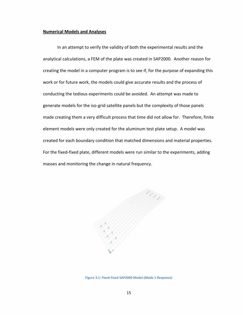
Numerical Models and Analyses
In an attempt to verify the validity of both the experimental results and the
analytical calculations, a FEM of the plate was created in SAP2000. Another reason for
creating the model in a computer program is to see if, for the purpose of expanding this
work or for future work, the models could give accurate results and the process of
conducting the tedious experiments could be avoided. An attempt was made to
generate models for the iso-grid satellite panels but the complexity of those panels
made creating them a very difficult process that time did not allow for. Therefore, finite
element models were only created for the aluminum test plate setup. A model was
created for each boundary condition that matched dimensions and material properties.
For the fixed-fixed plate, different models were run similar to the experiments, adding
masses and monitoring the change in natural frequency.
Figure 3.1: Fixed-Fixed SAP2000 Model (Mode 1 Response)
16
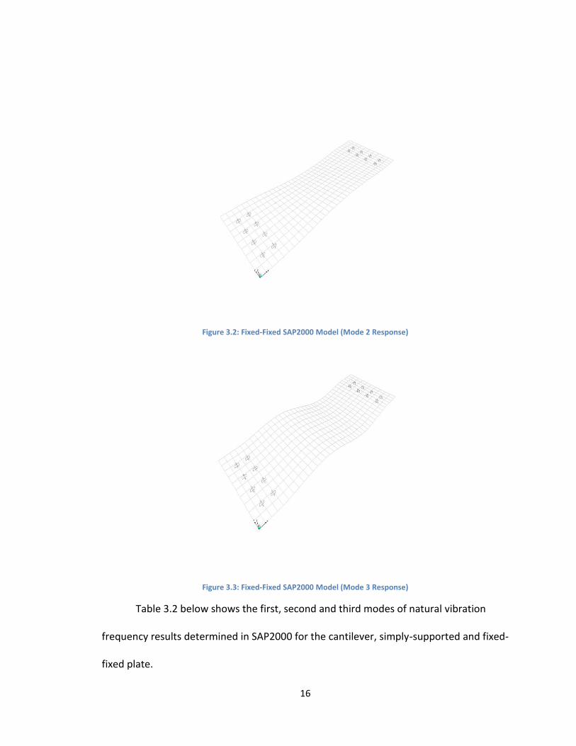
Figure 3.2: Fixed-Fixed SAP2000 Model (Mode 2 Response)
Figure 3.3: Fixed-Fixed SAP2000 Model (Mode 3 Response)
Table 3.2 below shows the first, second and third modes of natural vibration
frequency results determined in SAP2000 for the cantilever, simply-supported and fixed-
fixed plate.

17
Table 3.2: SAP2000 Results for Each Boundary Condition
Cantilever Plate (Hz) Simply-Supported Plate
(Hz) Fixed-Fixed Plate (Hz)
Mode 1 Mode 1 Mode 1
ω 13.98 ω 49.70 ω 112.79
Mode 2 Mode 2 Mode 2
ω 69.08 ω 164.15 ω 184.27
Mode 3 Mode 3 Mode 3
ω 87.09 ω 191.40 ω 309.43
To simulate the added masses in the experiments, masses were added to the
computer model to determine the resulting frequencies. Table 3.3 below shows the
frequencies obtained for the first three modes of the fixed-fixed plate when adding
mass to it.

18
Table 3.3: SAP2000 Results for Adding Masses to Fixed-Fixed Plate
SAP2000 Results for Fixed-Fixed Plate with Mass
Mass (g) Mode Frequency (Hz)
0
1 112.79
2 184.27
3 309.43
1
1 113.11
2 184.27
3 309.46
2
1 112.8
2 184.24
3 309.43
5
1 111.89
2 184.15
3 309.37
10
1 110.42
2 184.01
3 309.27
20
1 107.62
2 183.75
3 309.07
50
1 100.25
2 183.03
3 308.48
100
1 90.6
2 182.02
3 307.59
Discussion
Comparing Table 3.1 and 3.2, it can be seen that the frequencies obtained from
the FEM analyses for the first mode of each boundary condition case are very similar to
the analytical solutions (less than 1% difference). The fundamental frequencies were

19
also similar to that of the tests reported earlier (except for the simply-supported case
for reasons discussed earlier). The results for the cantilever beam are almost identical
and that of the fixed-end condition show just a slight difference in value that could be
attributed to difficulty in attributing an exact length to a fixed-end condition created by
two rows of bolts
The first modes from the FEM analyses (bending mode, Figure 3.1) shown in
Table 3.3 are very similar to the test results reported in Table 3.6 later on in the chapter.
The 2nd mode in the FEM analyses corresponds to a torsional mode (Figure 3.2) which
was not considered in the analytical solutions. The results obtained for mode 3 (the
second bending mode, Figure 3.3) with SAP2000 are very similar to the results
calculated for the corresponding 2nd bending mode by the analytical solutions for each
respective boundary condition.
Following are the experimental results obtained from the three different
boundary conditions on the aluminum plate.
Cantilever Plate
An attempt to replicate the effects on a cantilever beam was created by
removing all 8 bolts at one end and tightening the 8 bolts at the opposite end. To avoid
removing and re-attaching the accelerometer to the plate multiple times, the
accelerometer remained attached in the center of the plate during the testing on the
cantilever plate, where it was best located while measuring with the other two
boundary condition cases. For the simply supported and fixed-fixed cases, having the

20
accelerometer in the middle of the plate (directly between the nodes) allowed for the
most precise modal measurements, considering the center of the plate would
experience the largest deflection. Although the center of the plate was the most ideal
location for 1st mode response, it was the location of a node for the 2nd mode which
resulted in little to no response. Therefore, only the fundamental frequency for the
aluminum plate was analyzed. Given the large relative deflections of the cantilever
plate, the centrally-located accelerometer still provided accurate vibration response
data.
The free end of the plate was tapped with the rubber mallet and a natural
vibration frequency was recorded. There were consistently three different frequencies
that occurred: 13.8, 69, and 83 Hz. It became evident the frequency of 13.8 Hz
corresponded to the first resonant mode, 69 Hz to the second mode and 83 HZ to the
third mode. Comparison of this data to analytical and finite element modeling is
discussed later herein..
Pseudo-Simply Supported Plate
Using the bolts to attach the ends of the plate made it difficult to simulate the
simply-supported boundary condition. One row of 4 bolts was removed on each end of
the plate leaving a single row of 4 bolts. The bolts were loosened to a certain degree,
such that a small rotation could occur. A simply-supported condition could not be
accurately replicated because even though the bolts allowed for some rotation, they
restricted all translation at both ends. It is my opinion this is the reason the results of

21
this condition were not as close to the analytical solution and the computer models as
the cantilever and fixed conditions. The dominant first-mode frequency seen during the
testing fell in the range of 60-80 Hz.
The frequencies measured during the testing of the simply supported plate were
inconsistent. As one might expect, the tightness of the bolts would affect the stiffness
of the plate and in this particular case, changing the tightness of the bolts resulted in a
frequency variance of roughly 20 Hz. The following figures show how the experimental
data was gathered for the response of an impacted simply-supported plate using
Labview.

22
Figure 3.4: Impact Response of a Pseudo Simply Supported Plate
Figure 3.5: Frequency Spectrum for the Pseudo Simply Supported Plate (Linear Scale)
Figure 3.6: Zoomed Section of the Dominant Frequency on Pseudo Simply Supported Plate
Acc
ele
rati
on
, g
Am
plit
ud
e A
mp
litu
de

23
Fixed-Fixed Plate
The fixed-fixed plate boundary condition was used for a majority of the testing
because it is believed to be the closest replication of the actual condition of a satellite
panel. With the accelerometer still attached to the center of the plate and the
excitation of the plate brought on by an impact at the center with a rubber mallet, a
consistent dominant frequency was evident. A series of tests were done with the setup
sitting on top of a desk in the structures lab at the University of New Mexico (location 1)
and then the setup was moved to a desk top in an office (location 2) and then it was
moved to the floor in the same office (location 3). Table 3.4 shows the results obtained
when the setup was tested at locations 1 and 2 and table 3.5 shows the results obtained
when the setup was at location 3.
Table 3.4: Average Natural Frequencies of Aluminum Test Panel at Locations 1 & 2
Fixed-Fixed Aluminum Plate Natural Frequency Averages (location 1 & 2)
Date Average Std. Dev.
2/5/2010 113.4 0.30
2/26/2010 113.7 0.06
3/14/2010 119.8 2.06
4/9/2010 113.9 1.87
4/10/2010 114.5 2.72
10/2/2010 111.5 0.60
10/3/2010 113.7 0.98
11/13/2010 116.1 0.04
11/26/2010 113.0 5.18
11/28/2010 116.1 1.73
12/3/2010 114.1 0.42
12/18/2010 117.6 0.34
12/19/2010 115.9 0.41
1/8/2011 118.0 0.91

24
Table 3.5: Average Natural Frequencies of Aluminum Test Panel at Location 3
Fixed-Fixed Aluminum Plate Natural Frequency Averages (location 3)
Date Average Std. Dev.
1/9/2011 124.1 2.92
1/10/2011 125.6 0.49
1/11/2011 126.0 0.40
1/12/2011 125.3 0.40
1/13/2011 124.8 0.49
1/15/2011 125.2 2.15
1/16/2011 125.7 2.03
1/17/2011 122.4 0.54
1/18/2011 121.9 0.29
1/19/2011 123.4 0.55
1/22/2011 122.9 1.49
1/30/2011 123.9 0.27
Some of the test results shown above represent an analysis where a full day of
testing was performed and some represent an analysis of data for just a segment of
time that testing could be performed on that day (i.e. 5 pm – 10 pm). The testing done
for a full day is distinguishable by the higher standard deviations. Testing on the
aluminum plate showed the natural frequency would tend to fall throughout the course
of the day. The drop was not uniform but it was consistent and tended to follow a
pattern. It was ultimately determined that temperature played a role in the fluctuation
of the frequencies, however there was not a direct correlation due to the effect of the
behaviors of both the aluminum test plate and the steel base plate under changing
temperatures. A more detailed explanation of the temperature effects is discussed later
in the chapter.

25
As seen in the difference in results from Table 3.4 to Table 3.5, there was a
substantial difference in the natural frequencies obtained based on location of the test
set-up in the laboratory. From the beginning of the testing it was believed that the
steel base would provide a sturdy foundation and prevent vibration from transmitting
through it, into the substrate and ultimately having an effect on the results. Moving the
setup from the desk top to the floor was an attempt to test that theory.
Shown below is the response signal upon impact of the fixed-fixed plate followed
by the results of a fast Fourier transform showing the dominant frequency followed by a
zoomed in area of what’s shown in Figure 3.8.

26
Figure 3.7: Impact Response of the Fixed-Fixed Plate
Figure 3.8: Frequency Spectrum of the Fixed-Fixed Plate (Linear Scale)
Figure 3.9: Zoomed Section of the Dominant Frequency on Fixed-Fixed Plate
Acc
ele
rati
on
, g
Am
plit
ud
e A
mp
litu
de

27
Temperature Effects
Throughout the testing of the aluminum plate, the natural vibration frequencies
measured would change throughout the course of the day. The frequencies would start
out high and gradually decline throughout the day and only begin rising during the night.
See figure 3.10 for a graphical representation of this occurrence. Each time a full day of
testing was performed, this same pattern was seen. As one would expect, the
temperature of the plate would fluctuate throughout the course of the day, typically
beginning low and then rising until mid-afternoon at which point it would usually
plateau and hold constant for a period of time. Later in the evening the temperature
would begin dropping and would continue into the night before cycling through the
process again. The temperature of the aluminum plate would also follow this same
pattern.

28
Figure 3.10: Frequency Values for 10 Days of Testing
An aluminum plate was used in this testing because aluminum alloy is the most
commonly used metal for spacecraft structures (Larson and Wertz, 1999). The
temperature effect can be attributed to the differential expansion of the aluminum,
compared to that of the steel base, and the thermal inertial of the two metals with
different size which leads to variation in the constraints on the plate.
A set of experiments were conducted to purposely change the temperature of
the test set-up to verify this effect. Once the plate was heated up to about 80 degrees,
vibration tests were conducted resulting in a natural frequency was much lower than
prior to the plate being heated. The frequency drop was roughly 40 Hz with just a 5
degree increase in temperature. Tests were continued while the plate cooled back off
120
121
122
123
124
125
126
127
128
129
130
Fre
qu
en
cy (
Hz)
1 2 3 4 5 6 7 8 9Days
29
to room temperature and the frequency showed instant changes, rebounding
consistently with the dropping temperature.
Statistical Analysis
The criterion applied to determine if a mass is detectable on the plate was a 1-
standard deviation separation from the base-line (no mass), hence, the mean obtained
for a series of tests for a specific mass must fall outside of the range of one standard
deviation of the mean of the plate with no mass on it. The range of mass added to the
plate was from 1 to 100 grams early on in the testing and then a separate set of masses
were obtained which allowed for testing from 0.8 to 100 grams, with smaller increments
on the lower end. Determining a natural frequency for the plate with a 100 gram mass
attached was fairly difficult as that much mass usually damped the vibration too quickly
to determine a frequency. Given this, 100 grams was the upper limit of testing for the
aluminum plate.
Additional insight as to the use of 1 standard deviation as the detectability
criteria is as follows. The Hypothesis that is subject to statistical analysis is that ‘the
added mass results in a frequency shift’. In order to determine the confidence level for
this hypothesis to be accepted, one needs to evaluate how the average frequency with
the added mass differs from the average frequency of the baseline (no mass added),
μ. The standard deviation of the frequency data with no added mass is σ. To determine
the confidence level it is necessary to evaluate the value of Z which relates the
separation of the average frequencies to the standard deviation of the baseline:

30
(Equation 3.10)
Here is the average frequency with the added mass from n data points (tests). The
value of Z provides the basis for confidence interval assuming a normal distribution of
the data. Using a 1-standard deviation difference as the criteria for detectability implies
that , hence Z = . If n = 10 (there were at least 10 data points with the
added mass), then the probability of Type I error (determination of added mass when
there is none) is only 0.08% (based on 1-tailed Z functions since added mass can only
lead to a decrease in the frequency). A larger number of samples will further reduce the
error while a smaller number of samples will increase the error and decrease the
confidence interval (just 1 sample, n = 1 will result in 16% probability of type 1 error).
Analysis of Aluminum Test Plate Results
The testing done at locations 1 and 2 did not have any temperature recorded
because it wasn’t until later on that the realization was made that temperature might be
a factor. Therefore, shown below (Table 3.6 and Figure 3.11) is one set of analyses from
the results obtained from testing at location 1 without any temperature data present.
The averages shown in Table 3.6 are a result of 30 or more tests at each listed mass. A
second set of results obtained from location 3 with temperature data will be presented
subsequently. Table 3.6 shows the averages and one standard deviation for the results
obtained on testing of the blank plate and with a series of 7 different masses. Figure

31
3.11 shows the average of each different test and also shows the range determined by
one standard deviation of the mean.
Table 3.6 Statistical Results of Testing at Location 1
Mass (g) Average Std. Dev.
0 113.8 1.20
1 113.2 1.84
2 113.1 1.94
5 111.7 0.24
10 111.5 1.95
20 109.2 2.01
50 102.6 0.41
100 86.0 7.60
Figure 3.11: Frequency Ranges to One Standard Deviation for Each Mass
From figure 3.11, you can see that beginning at about 5 grams, the mean
frequency has shifted sufficiently far as to determine that anything 5 grams or greater
75.00
80.00
85.00
90.00
95.00
100.00
105.00
110.00
115.00
120.00
0 1 2 5 10 20 50 100
Fre
qu
en
cy (
Hz)
Mass (g)

32
would be detectable using the given evaluation criteria. Tests were also run with 200
and 500 gram masses on the plate but this much weight caused the vibration to dampen
out too quickly and no distinguishable frequency could be recorded.
When it was observed that the frequencies were falling throughout the day, the
temperature of the plate was recorded during testing to see if there was a thermal
effect. In an attempt to troubleshoot the issues regarding the daily fall in frequencies,
temperature data was only recorded when testing with no mass on the plate.
Additionally, the frequency testing with mass was done during the periods of time when
the plate temperature had stabilized in an attempt to remove the thermal effects from
the frequency deviations. Table 3.6 and Figure 3.12 below show the results of testing
with mass along with two different scenarios with no mass on the plate. Again,
averages shown are a result of 30 or more tests at each listed description.
Table 3.7: Test Results for Aluminum Plate with Added Masses
Description Average (Hz) Standard Deviation
ΔT(°F)
All temperature recorded data (no mass) 124.3 2.16 16
7 days from the same time period (5pm -9pm) (no mass)
124.6 1.48 10
0.8 grams mass added to plate 123.8 0.06 -
1.4 grams of mass added to plate 123.6 0.09 -
3.6 grams of mass added to plate 123.3 0.48 -
7.4 grams of mass added to plate 123.0 0.20 -
14.8 grams of mass added to plate 121.5 0.78 -
18.4 grams of mass added to plate 120.6 0.13 -
29.6 grams of mass added to plate 120.0 0.05 -
37.1 grams of mass added to plate 118.6 0.18 -
59.1 grams of mass added to plate 113.4 0.05 -
100 grams of mass added to plate 105.8 0.14 -

33
Figure 3.12: Frequency Ranges to One Standard Deviation for Each Mass Compared to Blank Plate Temperature Cycles
The first row of data in Table 3.7 combines all of the testing that was done once
temperature began being recorded and it can be seen that throughout that time period,
the temperature varied by 16 degrees. This was shown in an attempt to determine
what range of fluctuation could be attributed to temperature fluctuation rather than to
the added mass. In an attempt to reduce the influence of temperature fluctuation, a
smaller window of time was analyzed which resulted in a smaller variance in
temperature. For many days, testing was only done in the evenings from approximately
5 pm to 9 pm. This resulted in a temperature range of 10 degrees and as expected, a
smaller standard deviation (Table 3.7).
Figure 3.12 can also be analyzed by investigating the results of testing when
temperature fluctuation is eliminated. The standard deviations are sufficiently low that
a mass of 7.4 grams can be distinguished from an added mass of only 0.8 grams (or no
104.00
109.00
114.00
119.00
124.00
0 0 0.8 1.4 3.6 7.4 14.8 18.4 29.6 37.1 59.1 100
Fre
qu
en
cy (
Hz)
Mass (g)
ΔT = 16
ΔT = 10

34
added mass). When comparing the frequencies of the plate with masses added to the
blank plate testing that saw a temperature range of 16 degrees, the first mass that falls
outside of one standard deviation (and hence considered detectable) is 14.8 grams.
Each subsequent mass also fell outside of the range of one standard deviation. When
the blank plate saw a temperature variation of 10 degrees, the detectable mass did fall,
but not as much as expected, to 7.4 grams. Each subsequent mass was also detectable
for this case. This result can be compared to the first detectable mass of 5 grams from
tests at location 1 where no temperature data was taken. Hence, stability or
corresponding detection of temperature significantly improves detectability.
A satellite in orbit can typically expect to experience temperatures in the range
of -130°C and 100°C with changes occurring in minutes (Larson and Wertz, 1991).
Having seen what a temperature range of 16 degrees does to the modal behavior of an
aluminum plate, one can expect to see a much wider range of results when dealing with
a temperature range of over 200°C. There exists a thermal subsystem on the satellite
which manages the temperature of the equipment by means of the physical
arrangement of the equipment and using thermal insulation and coatings to balance
heat from power dissipation, absorption from the Earth and Sun, and radiation to space
(Larson and Wertz, 1991). Given all of this, it’s evident that thermal effects will play a
crucial role in any space structure health monitoring.

35
Chapter 4
SATELLITE TESTING
Testing on Satellite Panels
Vibration testing was done at the Air Force Research Lab Space Vehicles
Directorate on two different setups: A couple of iso-grid satellite panels and a mock
satellite.
PnP 2 Iso-Grid Satellite Panel
First, an accelerometer was placed on an aluminum satellite panel, called PnP 2,
which was attached at a 90 degree angle to a larger satellite panel, called PnP 1. PnP 1
was clamped down to a large table in an attempt to steady the setup as much as
possible. PnP 2 is an iso-grid aluminum alloy satellite panel that measures 0.5m x 1m
and PnP 1 is an iso-grid aluminum alloy satellite panel that measures 1m x 1m. The
mass of PnP 2 is roughly 7.80 kg and 17.42 for PnP 1. Figure 4.1 below shows a diagram
of the setup.

36
With the larger panel lying down on the table, the smaller panel acted as a
cantilever. The connection between the two panels consisted of 3 aluminum angles
which were bolted to each panel. This connection did not allow for rotation or
translation. The accelerometer was attached to the cantilever end of the smaller panel
which was also the end that was impacted with the rubber mallet. As mentioned, the
larger panel was bolted down to a large table to fix the entire setup. See Figures 4.2 and
4.3 showing photos of the setup.
Figure 4.1: PnP 2 Test Panel Setup
Accelerometer
PnP 2 Iso Grid
Aluminum
Panel (0.5m x
1m) PnP 1 Iso Grid Aluminum Panel (1m x 1m)
Mass bolted to panel
Location of Impact

37
Figure 4.2: Photo of PnP 2 Setup Showing Accelerometer Location
Figure 4.3: Photo Showing How the Setup was Clamped to the Table
Location of Impact

38
There were only a few different types and sizes of masses available for attaching
to the satellite panel due to the bolt pattern on the panel. These masses can be seen in
Figure 4.3 in the top right corner of the photo. Similar to the testing that was done on
the aluminum plate setup, frequency testing of the satellite panel was performed with
no mass present and then with increasing masses. The following photo shows the
location that the masses were added.
Figure 4.4: Photo of PnP 2 Setup Showing a Mass Bolted to the Plate
Due to the testing being performed in a lab, the temperature, which was
checked, remained constant throughout the entire testing process. Therefore,
temperature data was not recorded with any of this testing. See results of testing on
PnP 2 below in Table 4.1.
Location of Impact

39
Table 4.1: Statistical Results of Testing on PnP 2
AFRL PnP 2 Iso Grid Panel
Mass (g) Average (Hz) Std. Dev. (Hz)
0 48.5 0.22
30.5 48.5 0.05
54 48.5 0.06
108 48.4 0.05
162 48.2 0.07
216 47.9 0.05
246.5 47.8 0.06
2819 43.7 0.11
2849.5 43.6 0.04
5678 40.0 0.13
Figure 4.5: Frequency Rangers to One Standard Deviation for PnP 2 Testing
As can be seen from Table 4.1 and Figure 4.5 above, a 2819 gram mass or greater
added to the panel has a substantial effect on the natural frequency of the panel and
would be easily detectable through this type of testing. A closer look at the data up to
39.00
40.00
41.00
42.00
43.00
44.00
45.00
46.00
47.00
48.00
49.00
0 30.5 54 108 162 216 246.5 2819 2849.5 5678
Fre
qu
en
cy (
Hz)
Mass (g)
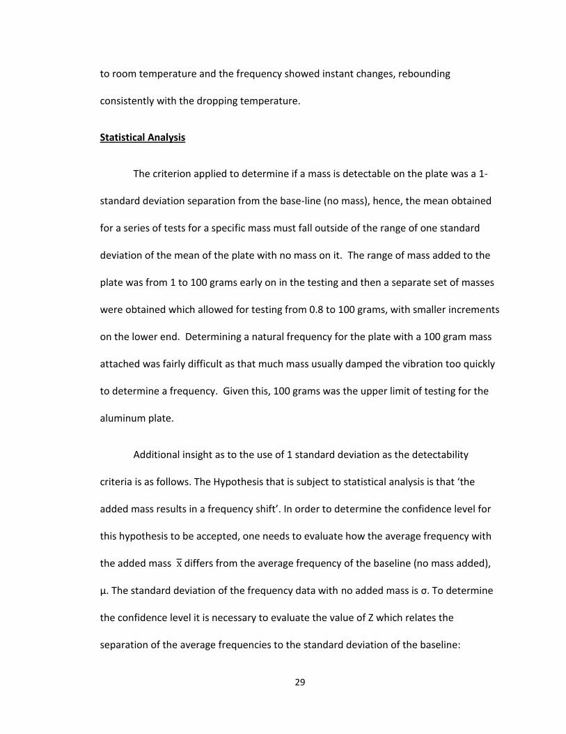
40
246.5 grams (Figure 4.6) shows that the 162, 216 and 246.5 gram masses fell well
outside the range of one standard deviation of the mean for the blank panel and would
be detectable in this scenario.
Figure 4.6: Frequency Ranges to One Standard Deviation for PnP 2 Testing from 0-246.5 grams
We can also see that 162 grams and greater is distinguishable from the baseline
condition per the evaluation criteria. One could argue that the shift in the mean
frequency between the baseline condition and 108 grams is sufficient enough to allow a
mass of 108 grams to be detectable.
Mock Satellite Testing
The second test setup at the Air Force Research Laboratory Space Vehicles
Directorate was a mock satellite. Six aluminum iso-grid satellite panels were erected in
the shape of a cube and dummy payloads were added on each side. The connection
47.60
47.80
48.00
48.20
48.40
48.60
48.80
0 30.5 54 108 162 216 246.5
Fre
qu
en
cy (
Hz)
Mass (g)

41
between each panel consisted of a hinge that effectively allows for rotation but not
translation. The weight of the mock satellite was not measured but roughly calculated
based on the known mass of the satellite panels PnP 1 and PnP 2, giving a mass of
approximately 66 kg. The following figure shows the basic configuration.
Dummy
Payloads
Accelerometer
Mass
added to
structure
Figure 4.7: Diagram of Mock Satellite Test Setup

42
Figure 4.8: Photo of Mock Satellite Test Setup with Mass Attached
Figure 4.9: Photo Showing Connection Between Panels on Mock Satellite
The mock satellite was the most practical application. However, it was also the
set-up where the least amount of testing was done due to other constraints. The bolt

43
pattern on this mock satellite did not match the bolt pattern on the PnP 2 satellite panel
or the bolt pattern for the available masses. Hence, there were only a few of the
masses that were actually available to be attached to the top panel. Table 4.2 shows
the results of the testing done on this structure.
Table 4.2: Statistical Results for Mock Satellite Testing
AFRL Mock Satellite
Mass (g) Average (Hz) Std. Dev. (Hz)
0 43.0 0.44
108 43.1 0.24
2819 40.1 0.25
5678 38.6 0.22
Figure 4.10: Frequency Range to One Standard Deviation for Mock Satellite Testing
Even though the connections between the panels on the mock satellite were
hinges that allowed for rotation, the structure as a whole was extremely rigid and it was
conjectured before testing began that the natural frequency of the panel may not be
38.00
39.00
40.00
41.00
42.00
43.00
44.00
0 108 2819 5678
Fre
qu
en
cy (
Hz)
Mass (g)

44
distinguishable from that of the structure. Fortunately, a natural frequency was seen
and as seen from the results, the addition of a mass did have affect on the vibration of
the structure. Unfortunately, there weren’t masses available to experiment with
between 108 grams and 2819 grams. From the graph, it can be seen that the
frequencies obtained with the presence of the 108 grams of mass fall directly with the
range of frequencies obtained with no mass present and therefore would not be
detectable. On the other hand, results obtained with the presence of 2819 grams of
mass are well outside of the range and thus easily detectable. Even though the size of
the detectable mass on the mock satellite couldn’t be narrowed down any further, the
overall goal of determining whether or not the addition of a mass could be detected
through vibration-based monitoring was successful.

45
Chapter 5
CONCLUSIONS
Conclusion
The three test setups (aluminum plate, PnP 2 and the mock satellite) each
provided their own unique opportunity to determine solutions from what could arise as
potential problems experienced while trying to do vibration-based testing on an orbiting
satellite. The aluminum plate provided the opportunity for large variety of testing and
also exposed the problem created by temperature fluctuations. The iso-grid panel PnP 2
enabled testing to be done on an actual satellite panel and the mock satellite allowed
for testing on a large-scale model of a satellite.
It was observed that the simply-supported case is difficult to emulate in the
laboratory due to the bolted connection. Other than the simply-supported case, the
results obtained by the computer model are similar to the experimental results and the
analytical solutions. Also explained was the difference in the solutions for the 2nd and
higher modes for analytical solutions versus the computer solutions; only the 1st mode
was used in subsequent analysis and interpretation – Providing a rigid support to the
test apparatus was also important as evident from conducting the tests on the floor vs.
on a table. Ultimately, the objective of determining the accuracy of a finite element
program to model the experimental data upon adding masses to the plate was
successful.

46
Compared to a mass of 740 grams for the aluminum plate, added mass as small
as 14.8 grams (approximately 2.0% of the weight of the plate) was detectable in spite of
temperature fluctuations. The detectability improved to 7.4 grams when temperature
fluctuation was eliminated. Based on these results, it becomes clear that more focus
needs to be directed towards reduction or measurement of the thermal effects on the
material behavior. This can lead to significant improvement in detectability. The
threshold of detectability on an actual satellite panel (PnP 2) was established through
testing.
As mentioned, 100 grams was the upper limit of mass detection on the
aluminum plate due to anything larger damping the vibration too quickly to observe a
natural frequency. This type of limit was not seen with the testing done on the Air Force
Research Laboratory Space Vehicles Directorate panels and satellite but one could
hypothesize that the upper limit may exist around 15-20% of the total mass of the
structure. Similar to the aluminum test plate, the minimum mass detectability on the
satellite panels and the mock satellite is a very small percentage of the total mass of the
structure.
Finite element models of the iso-grid panels and the mock satellite were not
within the scope of this research. However, results from the model of the aluminum
plate give confidence in the reliability of SAP2000 to accurately model the modal
behavior of a structure while adding masses.

47
Even though the fundamental frequencies of spacecrafts are usually known by
the launch vehicle contractor prior to launching the craft into orbit (Larson and Wertz,
1999), they may change slightly once in orbit. Determining the fundamental frequency
of the spacecraft once it goes into orbit becomes important because a baseline needs to
be identified. See Appendix B for lists of different satellites and their fundamental
frequencies.
Recommendations for Future Work
As mentioned, temperature effects on frequency response are an important
factor that must always be considered when doing vibration-based testing. This
research incorporated temperature data into the behavior of the aluminum plate but
only for a limited range. For any application on space structures, temperature must be
an integral part of the analysis and must incorporate a wide range of temperatures and
associated material behaviors. Taking into account the spacecraft’s thermal subsystem
would also be helpful in determining the typical temperature ranges a spacecraft should
expect to experience.
Changes in stiffness, whether local or distributed, lead to changes in the natural
frequencies of a vibrating system (Adams et al., 1978). Understanding that, there is a
concern of being able to make a distinction between an added mass and damage to a
structure when using FRF’s as a method of monitoring. One might expect damage and a
loss of mass to be the same thing and that a loss of mass might have the opposite effect
of an added mass. It was seen that an added mass would cause the vibration of the

48
structure to dampen out much quicker; therefore, a loss of mass may have the effect of
reduced stiffness and an increase in natural frequency of the structure. Either way, the
difference in the two scenarios presents an interesting focal point for future research.
By far the most interesting potential topic for future work involves methods of
testing satellite structures. Obviously, remote wireless monitoring is the only option
when dealing with a space structure. Wireless monitoring of a structure is nothing new
but what specifically becomes challenging with vibration-based monitoring is how to
excite the structure. Peteers et al. (2001) looked at different excitation sources on
vibration-based structural health monitoring of bridge, as well as temperature effects.
He investigated the difference in using normal traffic flow, mass shakers, a drop weight
and ambient sources such as wind or earthquakes. When operating in space, excitation
of a structure becomes much more complex. There are so-called natural sources of
excitation such as impacts with other objects. A satellite can be bombarded with the
surrounding atmosphere at orbital velocities on the order of 8 km/s (Larson and Wertz,
1999). The only other apparent option would be to generate the excitation somehow.
Spacecrafts have thrusters and various methods of propulsion for orientation purposes
that could be viable sources of excitation. There has also been research done into the
use of Piezoceramic (PZT) actuator-sensor as both and excitation and data gathering
sensor (Ritdumrongkul et al. (2003, 2004) and Tanner et al. (2003)).

49
Appendix A: Material Properties for the Aluminum Test Plate
Material
Alloy
ρ
(lb/in3)
Ftu
(103 lb/in2)
Fcy
(103 lb/in2)
E
(106 lb/in2)
e
(%)
α
(10-6/°F)
6061-T6 Aluminum 0.098 42 35 9.9 10 12.7
ρ = density
Ftu = Allowable Tensile Ultimate Stress
Fcy = Allowable Compressive Yield Stress
E = Modulus of Elasticity
e = Elongation
α = Coefficient of Thermal Expansion

50
Appendix B: Fundamental Frequencies for Various Satellites
From Larson and Wertz (1999):
Launch System Fundamental Frequency (Hz)
Axial Lateral
Atlas II, IIA, IIAS 15 10
Ariane 4 31 10
Delta 6925/7925 35 15
Long March 2E 26 10
Pegasus, XL 18 18
Proton 30 15
Space Shuttle 13 13
Titan II 24 10

51
References
Wu Z., Qing X., P., Chang F., (2009), “Damage Detection for Composite Laminate Plates
with A Distributed Hybrid PZT/FBG Sensor Network. Journal of Intelligent Material
Systems & Structures, Vol. 20 Issue 9, p1069-1077
Qing, X. P.; Beard, S. J.; Kumar A., Teng K. O., Chang F. (2007), “Built-in Sensor Network
for Structural Health Monitoring of Composite Structure”, Journal of Intelligent Material
Systems & Structures, Vol. 18 Issue 1, p39-49.
Tanner, Neal A., Wait, Jeannette R., Farrar, Charles R., and Sohn, Hoon, (2003)
“Structural Health Monitoring Using Modular Wireless Sensors.” Journal of Intelligent
Material Systems and Structures, 14, 43-56.
Wertz, James R. and Larson, Wiley J. (1991). Space Mission Analysis and Design, 3rd
Edition, Microcosm Press, El Segundo, CA.
Adams R. D., Cawley P., Pye C. J. and Stone B. J. (1978). A vibration technique for non-
destructively assessing the integrity of structures. Journal of Mechanical Engineering
Science. 20, 93-100.
Zang, C., Friswell, M. I., and Imregun, M. (2007). “Structural Health Monitoring and
Damage Assessment Using Frequency Response Correlation Criteria.” Journal of
Engineering Mechanics, 133(9), 981-993.
Shi, Z. Y., Law, S. S., and Zhang, L. M. (2000). “Damage localization by directly using
incomplete mode shapes.” Journal of Engineering Mechanics, 126(6), 656-660.

52
Sampaio, R. P. C., Maia, N. M. M., Silva, J. M. M., and Almas, E. A. M. (2003). “Damage
Detection in Structures: From Mode Shape to Frequency Response Function Methods.”
Mechanical Systems and Signal Processing., 17(3), 489–498.
Peeters, Bart, Maeck, Johan, De Roeck, Guido, (2001). “Vibration-Based Damage
Detection in Civil Engineering: Excitation Sources and Temperature Effects.” Smart
Materials and Structures, 10(3), 518-527.
Chatterjee, A. (2010). “Structural Damage Assessment in a Cantilever Beam with a
Breathing Crack Using Higher Order Frequency Response Functions.” Journal of Sound
and Vibration, 329(16), 3325-3334.
Moreno, D., Barrientos, B., Perez-Lopez, C., Mendoza Santoyo, F., (2005). “Modal
Vibration Analysis of a Metal Plate by Using a Laser Vibrometer and the POD Method.”
Journal of Aptics A: Pure and Applied Optics, 7, S356-S363.
Botta, F., Cerri, G., (2007). “Shock Response Spectrum in Plates Under Impulse Loads.”
Journal of Sound and Vibration, 308, 563-578.
Chopra, Anil K. (2007). Dynamics of Structures: Theory and Applications to Earthquake
Engineering, 3rd Edition, Pearson Prentice Hall, Upper Saddle River, NJ.
Ritdumrongkul, S., Fujino, Y. (2006). “Identification of the Location and Level of Damage
in Multiple-Bolted-Joint Structures by PZT Actuator-Sensors.” Journal of Structural
Engineering, 132(2), 304-311.

53
Ritdumrongkul, S., Masato, A., Fujino, Y. Miyashita, T. (2004). “Quantitative Health
Monitoring of Bolted Joints Using a Piezoceramic Actuator-Sensor.” Smart Materials and
Structures, 13, 20-29.
Lee, U., Shin, J. (2002). “A Frequency-Domain Method of Structural Damage
Identification Formulated from the Dynamic Stiffness Equation of Motion.” Journal of
Sound and Vibration, 257(4), 615-634.


