UNIVERSITY OF CALIFORNIA, SAN DIEGO
Autocorrelation Analysis of Spectral Regrowth Generated by
Nonlinear Circuits in Wireless Communication Systems
A dissertation submitted in partial satisfaction of the
requirements for the degree Doctor of Philosophy
in Electrical Engineering (Electronic Circuits & Systems)
by
Kevin Gard
Committee in charge:
Professor Lawrence Larson, Chair Professor Peter Asbeck Professor Chung-Kuan Cheng Professor Bill Hodgkiss Professor Paul Yu
2003

Copyright
Kevin Gard, 2003
All rights reserved

iii
SIGNATURE PAGE
The dissertation of Kevin Gard is approved, and it is
acceptable in quality and form for publication on
microfilm:
Chair
University of California, San Diego
2003

iv
DEDICATION
To my loving family:
Amanda, my lovely wife, for her love, support, and endurance.
Will, my son, for inspiring me to fulfill a childhood dream.
To my parents, Bill and Dorothy, for many years of love and support.

v
Table of Contents
Signature Page......................................................................................................iii
Dedication............................................................................................................iv
Table of Contents ..................................................................................................v
List of Figures ....................................................................................................viii
List of Tables........................................................................................................xi
Acknowledgements..............................................................................................xii
Vita, Publications, and Fields of Study................................................................xiv
Abstract of the Dissertation ................................................................................xvi
I. Introduction ...................................................................................................... 1
I.1 Adjacent Channel Interference ..................................................................... 4
I.2 Wireless Digital Communications................................................................. 8
I.3 Bandpass Nonlinearities..............................................................................12
I.4 Power Spectrum Estimation........................................................................15
I.5 Spectral Regrowth Analysis ........................................................................16
I.5.1 Transient Analysis of Spectral Regrowth..............................................17
I.5.2 Harmonic Balance Analysis of Spectral Regrowth................................18

vi
I.5.3 Envelope Simulation of Spectral Regrowth ..........................................21
I.5.4 AM-AM, AM-PM Modeling of Spectral Regrowth..............................23
I.5.5 Volterra Series Modeling of Spectral Regrowth ...................................25
I.5.6 Statistical Analysis of Spectral Regrowth .............................................26
I.5.7 Summary .............................................................................................27
I.6 Dissertation Organization ...........................................................................29
II. Autocorrelation Analysis of Bandpass Nonlinearities .......................................32
II.1 Bandpass Nonlinearity Analysis .................................................................33
II.2 Autocorrelation Analysis of Spectral Regrowth .........................................38
II.3 Crossmodulation Distortion.......................................................................50
II.4 Second-Order Interaction..........................................................................53
II.5 Nonlinear Models......................................................................................54
II.6 Power Series Model ..................................................................................63
II.7 Spectral Results.........................................................................................69
II.8 Summary...................................................................................................80
III. Statistical Analysis of Bandpass Nonlinearities ...............................................82
III.1 Statistical Moments..................................................................................83
III.2 Gaussian Random Process........................................................................85
III.3 Transformation of a Complex Random Process ........................................85
III.4 Transformation of a Bandpass Random Process .......................................90
III.5 Transformation of a Complex Bandpass Random Process.........................95

vii
III.6 Spectral Results .......................................................................................99
III.7 Summary ...............................................................................................110
IV. Simulation and Measurements......................................................................112
IV.1 Envelope Simulation ..............................................................................112
IV.2 AM-AM AM-PM Characterization ........................................................115
IV.3 ACPR Measurements.............................................................................125
IV.4 Summary ...............................................................................................128
V. Conclusions ..................................................................................................130
V.1 Future Work ...........................................................................................130
V.1.1 Distortion Analysis ...........................................................................131
V.1.2 Wireless System Analysis .................................................................132
V.1.3 Behavioral Modeling ........................................................................132
Appendix A: Power Series Coefficients for Limiter Models...............................134
Appendix B: MATLAB Code ...........................................................................137
References.........................................................................................................145

viii
LIST OF FIGURES
Figure I-1: CDMA handset transmitter block diagram................................................. 3
Figure I-2: Typical operation of mobile stations within a cellular network. .................. 4
Figure I-3: Adjacent channel interference.................................................................... 5
Figure I-4: Definition of adjacent channel power ratio................................................. 7
Figure I-5: Amplitude PDF for CDMA and Gaussian modulation signals. ..................12
Figure I-6: Transient simulation of modulated carrier.................................................18
Figure I-7: Circuit partitioning for harmonic balance analysis. ....................................20
Figure I-8: Envelope simulation of modulated carrier.................................................23
Figure II-1: Block diagram of quadrature modulator and bandpass nonlinearity..........34
Figure II-2: CDMA Signal construction and autocorrelation estimate. .......................41
Figure II-3: Real part of autocorrelation for OQPSK and QPSK IS-95 signals. ..........43
Figure II-4: Real part of autocorrelation for real and complex Gaussian signals..........43
Figure II-5: Imaginary part of autocorrelation for IS-95 signals. ................................44
Figure II-6: Imaginary part of autocorrelation for Gaussian signals. ...........................44
Figure II-7: Gain compression/expansion and distortion spectrum terms. ...................48
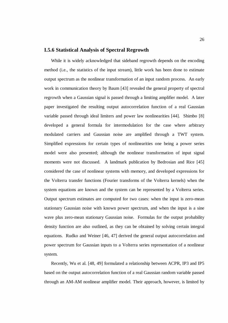
Figure II-8: Transfer characteristic for limiter models. ...............................................56
Figure II-9: Carrier transfer characteristic for limiter models. .....................................56
Figure II-10: Bipolar differential pair amplifier...........................................................59
Figure II-11: Multi-tanh triplet differential amplifier...................................................61
Figure II-12: Carrier gain compression characteristics for nonlinear models. ..............62
Figure II-13: Quadrature AM-AM AM-PM model.....................................................63
Figure II-14: Least squares and Taylor series expansion of Ltanh(ving/L). .................68
Figure II-15: Carrier gain characteristic of power series limiter models. .....................68
Figure II-16: Flow chart for power spectrum calculation............................................70

ix
Figure II-17: Spectrum components from autocorrelation analysis. ............................72
Figure II-18: Total output power spectrum at 6 dBm for each limiter model. .............73
Figure II-19: Distortion spectrum at 6dBm output power for each limiter model........73
Figure II-20: Adjacent channel power at 885 kHz offset for limiter models. ...............78
Figure II-21: Adjacent channel power at 1.98 MHz offset for limiter models..............78
Figure II-22: Slope of ACPR versus output power. ...................................................79
Figure II-23: CDMA Gain compression characteristic................................................79
Figure III-1: Power spectrum at 2 dBm with complex Gaussian input signal. ...........101
Figure III-2: Distortion spectrum at 2 dBm with complex Gaussian input signal.......101
Figure III-3: Spectrum from Gaussian moment and autocorrelation methods. ..........102
Figure III-4: Complex Gaussian ACPR1 sweep. ......................................................106
Figure III-5: Real Gaussian ACPR1 sweep. .............................................................107
Figure III-6: Complex Gaussian ACPR2 sweep. ......................................................107
Figure III-7: Real Gaussian ACPR2 sweep. .............................................................108
Figure III-8: Slope of ACPR for complex Gaussian input signal...............................108
Figure III-9: Complex Gaussian gain compression characteristic. .............................109
Figure III-10: Comparison of ACPR for different input signals. ...............................110
Figure IV-1: CDMA autocorrelation and envelope simulation results.......................114
Figure IV-2: Complex Gaussian autocorrelation and envelope simulation results......115
Figure IV-3: Measurement setups for AM-AM AM-PM characterization.................116
Figure IV-4: Schematic diagram of 900MHz driver amplifier. ..................................117
Figure IV-5: Measured AM-AM response of 900 MHz CDMA amplifier.................118
Figure IV-6: Measured AM-PM response of 900 MHz CDMA amplifier. ................118
Figure IV-7: Block diagrams of RFIC transmitter devices. .......................................120
Figure IV-8: RFIC transmitter measurement setup...................................................120
Figure IV-9: Cell band AM-AM AM-PM for superheterodyne RFIC. ......................123

x
Figure IV-10: PCS band AM-AM AM-PM for superheterodyne RFIC.....................123
Figure IV-11: Cell band AM-AM AM-PM for direct conversion RFIC. ...................124
Figure IV-12: PCS band AM-AM AM-PM for direct conversion RFIC. ..................124
Figure IV-13: Modeled and measured AM-AM/AM-PM for CDMA amplifier. ........126
Figure IV-14: Measured and calculated ACPR for CDMA reverse link signal. .........127
Figure IV-15: Measured and calculated ACPR for complex Gaussian input signal....128

xi
LIST OF TABLES
Table I-1: Adjacent channel emissions limits for CDMA and WCDMA mobile
transmitters......................................................................................................... 5
Table I-2: Decibel peak to average ratio for CDMA and Gaussian signals. .................12
Table I-3: Comparison of methods to analyze spectral regrowth. ...............................29
Table II-1: Comparison of sinusoidal P1dB input gain compression..............................62
Table II-2: Comparison of CDMA P1dB input gain compression. ................................77
Table III-1: Comparison of Gaussian P1dB input gain compression............................106
Table IV-1: Complex power series coefficients for 900 MHz CDMA amplifier. .......125

xii
ACKNOWLEDGEMENTS
I would like to take a moment to graciously thank all the folks who made it possible
for me to complete this dissertation. It is only through the inspiration, encouragement,
and understanding of others that I could bring this work to fruition.
First and foremost, I would like to express my sincere appreciation to my advisor
Professor Larry Larson and Professor Michael Steer of North Carolina State
University. Larry and Michael provided me with the guidance, wisdom,
encouragement, and fortitude to pursue and successfully complete this body of work.
I would also like to thank my Ph.D. committee members, Peter Asbeck, Paul Yu,
Bill Hodgkiss, and Chung-Kuan Cheng for their valuable comments and
recommendations regarding this dissertation.
A special round of thanks goes to my colleagues in the RF, PA, and RFIC design
fields whose conversations and debates about the origins of spectral regrowth
motivated much of my interest in the field. I would especially like to acknowledge:
Vladimir Aparin, John Sevic, Steve Kenney, Paul Draxler, Brett Walker, Hector
Gutierrez, and Khaled Gharaibeh.
I thank my lovely wife Amanda for her love, encouragement, and tolerance
throughout this long endeavor. And to my son, William, for his ability to make me
smile at anytime and for making me realize that reaching for your childhood dreams is
what life should be about. Last, but not least, I thank my parents for supporting me
always and teaching me that I should strive to be all that I can be.
This research was supported by QUALCOMM Inc.
The text of Chapters II, III, and IV in this dissertation, in part or in full, is a reprint
of the material as it appears in our published papers or as it has been submitted for
publication in IEEE Transactions on Microwave Theory and Techniques, Proceedings

xiii
of the IEEE International Microwave Symposium, and Proceedings of the IEEE
Custom Integrated Circuits Conference. The dissertation author was the primary author
listed in these publications directed and supervised the research which forms the basis
for these chapters.

xiv
VITA 1987 A.A.S. Durham Community College, Durham, N.C. 1985-1991 Electronic Engineering Technician, Raleigh, N.C. 1994 B.S., North Carolina State University, Raleigh, N.C. 1995 M.S., North Carolina State University, Raleigh, N.C 1996-2003 Electrical Engineer, Qualcomm Inc., San Diego, CA 2003 Ph.D., University of California, San Diego, CA 2004 Assistant Professor, North Carolina State University, Raleigh, N.C
VITA, PUBLICATIONS, AND FIELDS OF STUDY
PUBLICATIONS
K. Gard, L.E. Larson, M.B. Steer, “Autocorrelation Analysis of Spectral Regrowth from Wireless Circuits,” submitted for publication in the IEEE Trans. on Microwave Theory and Tech. K. Gard, L.E. Larson, M.B. Steer, “AM-AM and AM-PM Measurement of Baseband to RF Integrated Circuits for ACPR Calculations,” 2003 IEEE Radio and Wireless Conference, pp. 273-276. K. Gard, L.E. Larson, M.B. Steer, “Generalized Autocorrelation Spectral Regrowth From Bandpass Nonlinear Circuits, 2001 IEEE Int. Microwave Symposium,” vol. 1, pp. 9-12. K. Gard, L.E. Larson, M.B. Steer, “Autocorrelation Analysis of Distortion Generated From Bandpass Nonlinear Circuits,” 2001 IEEE Custom Integrated Circuits Conference, pp. 345-348. K. Gard, L.E. Larson, M.B. Steer, “Bandpass Techniques for Modeling and Analyzing Spectral Regrowth,” 2000 Santa Clara Valley MTT-S Workshop, pp. 153-179. H. Gutierrez, K. Gard, M.B. Steer, “Nonlinear Gain Compression in Microwave Amplifiers Using Generalized Power-Series Analysis and Transformation of Input Statistics,” IEEE Trans. on Microwave Theory and Tech., vol. 48, Oct. 2000, pp. 1774-1777. K. Gard, H. Gutierrez, M.B. Steer, “Characterization of Spectral Regrowth in Microwave Amplifiers based on the Nonlinear Transformation of a Complex Gaussian Process,” IEEE Trans. on Microwave Theory and Tech., vol. 47, July 1999, pp. 1059-1069.

K. Gard, M.B. Steer, “Efficient Simulation of Spectral Regrowth Using Nonlinear Transformation of Signal Statistics,” 1999 IEEE Topical Workshop on Power Amplifiers for Wireless Communications. H. Gutierrez, K. Gard, M.B. Steer, “Spectral Regrowth in Microwave Amplifiers Using Transformation of Signal Statistics,” 1999 IEEE Int. Microwave Symposium, vol. 3, pp. 985-988. K. Gard, H. Gutierrez, M.B. Steer, “A Statistical Relationship for Spectral Regrowth in Digital Cellular Radio, 1998 IEEE Int. Microwave Symposium,” vol. 2, pp. 989-992.
FIELDS OF STUDY
Major Field: Electrical Engineering
Studies in Circuit Design for Wireless Communications. Professor Lawrence Larson Studies in Circuit Simulation and RF Circuit Design. Professors Michael Steer, North Carolina State University Studies in Analog Integrated Circuit Design. Professor Ronald Gyurcsik, North Carolina State University

ABSTRACT OF THE DISSERTATION
Autocorrelation Analysis of Spectral Regrowth Generated by
Nonlinear Circuits in Wireless Communication Systems
by
Kevin Gard
Doctor of Philosophy in Electrical Engineering
University of California, San Diego, 2003
Professor Lawrence Larson, Chair
Modern wireless communication systems utilize sophisticated modulation
techniques to achieve higher data rates or improvements in overall system capacity.
Amplitude variations in the modulated waveforms give rise to distortion products when
applied to nonlinear components of the transmitter. Distortion emissions from mobile
handsets are limited to prevent system degradation and interference to users in adjacent
cells. However, there is an inherent tradeoff between transmitter efficiency and the
amount of distortion produced by the power amplifier. Thus when designing an
amplifier or transmitter component, it is important to quickly determine the distortion
generated by the circuit when a modulated signal is applied.

Estimation of spectral regrowth generated by a digitally modulated carrier passed
through a nonlinear RF circuit is analyzed using a formulation of the output
autocorrelation function. The estimation is based on developing an analytical
expression for the output power spectrum when the nonlinearity is modeled a complex
power series model extracted from measured amplitude-to-amplitude (AM-AM) and
amplitude-to-phase (AM-PM) characteristics. Comparisons are presented of measured
versus predicted ACPR values for a CDMA amplifier for CDMA and Gaussian signals.
A statistical technique is presented for the characterization of spectral regrowth at
the output of a nonlinear amplifier driven by a digitally modulated carrier in a digital
radio system. The technique yields an analytical expression for the autocorrelation
function of the output signal as a function of the statistics of the quadrature input signal
transformed by a behavioral model of the amplifier. The amplifier model, a baseband
equivalent representation, is derived from a complex radio-frequency envelope model,
which itself is developed from readily available measured or simulated amplitude
modulation–amplitude modulation and amplitude modulation–phase modulation data.
The statistical technique is used in evaluating spectral regrowth generated when
Gaussian signals are applied to nonlinear circuits.

1
I. Introduction
For the past twenty years, a revolution in the wireless industry has taken place.
Cellular phone technology has transitioned from bulky suitcase sized phones to palm
sized data phones with full color displays and internet surfing capabilities. This
revolution occurred, in part, from the implementation of digital cellular standards and
the development of high volume low cost components for developing digital cellular
phones. A key to success was the subsidizing of handset costs by the carriers in order
to raise the number of subscribers. The demand for low cost handsets pressures
handset manufactures to produce the lowest cost handset while still meeting all
performance requirements of the digital wireless standard. Therefore, product
performance tends to be stretched near the limits of the system requirement in order to
maximize handset yield.
Handset cost is a very complicated factor. For example, the manufacture of a
component is mainly concerned with maximizing the yield of one or more components
used in the system. Likewise, the phone manufacture is concerned with maximizing the
yields of phones. However, each component used must have specifications such that
the end product, a phone, is capable of being manufactured with high yields. This leads
to phone manufactures developing conservative component specifications to raise
confidence that phones will yield well. But the component manufacture will always
question the need for conservative component specifications in an effort to gain yield
margin for the components. Iterations continue until the cost and yield issues are
satisfied for both the component and phone manufactures.
A critical element to the performance requirement is the amount of undesired signal
strength that the handset transmitter is permitted to radiate outside of the transmission
bandwidth. Undesired products can be generated by multiple sources including

2
nonlinear distortion, mixing products, and spurious signals generated by phase locked
loops (PLL). These products can degrade the signal to noise ratio (SNR) of other
stations operating on the same frequency. Therefore, wireless cellular standards specify
maximum limits on the levels of undesired products allowed to keep the system
operational.
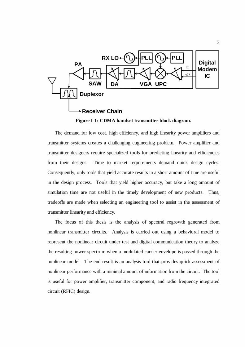
Modern transmitter systems consist of a radio frequency (RF) modulator, variable
gain amplifier (VGA), upconverter mixer (UPC), driver amplifier (DA), band select
filter, and power amplifier (PA) as shown in Figure I-1. Any one of these system
blocks is a source of nonlinear distortion; however, most emphasis is placed on the PA.
The power amplifier consumes the most amount of power from the battery, in the case
of a handset, or from the power line, in the case of a base station. Power efficiency of
the PA is a significant factor in determining the available "talk time" or battery life of a
handset or the monthly power bill cost of operating a basestation transmitter. High
efficiency operation of power amplifiers occurs when the amplifier is operated at its
maximum output power capacity; however, this requires driving the amplifier into a
highly nonlinear region of operation. Thus, the most difficult part of linear PA design is
achieving the highest efficiency possible without exceeding the linearity requirements.
Likewise, the phone designer should select the lowest cost power amplifier that
produces the highest efficiency without breaking the linearity specification.
3
DigitalModem
IC
PLLPLLRX LO
SAW
PA
Receiver Chain
Duplexor
VGA UPCDA
( )i t
( )q t
Figure I-1: CDMA handset transmitter block diagram.
The demand for low cost, high efficiency, and high linearity power amplifiers and
transmitter systems creates a challenging engineering problem. Power amplifier and
transmitter designers require specialized tools for predicting linearity and efficiencies
from their designs. Time to market requirements demand quick design cycles.
Consequently, only tools that yield accurate results in a short amount of time are useful
in the design process. Tools that yield higher accuracy, but take a long amount of
simulation time are not useful in the timely development of new products. Thus,
tradeoffs are made when selecting an engineering tool to assist in the assessment of
transmitter linearity and efficiency.
The focus of this thesis is the analysis of spectral regrowth generated from
nonlinear transmitter circuits. Analysis is carried out using a behavioral model to
represent the nonlinear circuit under test and digital communication theory to analyze
the resulting power spectrum when a modulated carrier envelope is passed through the
nonlinear model. The end result is an analysis tool that provides quick assessment of
nonlinear performance with a minimal amount of information from the circuit. The tool
is useful for power amplifier, transmitter component, and radio frequency integrated
circuit (RFIC) design.

4
I.1 Adjacent Channel Interference
Existing CDMA systems (IS-95, CDMA2000 1x, CDMA2000 EVDO) and future
WCDMA systems are full duplex systems where the transmitter and receiver operate
simultaneously at different frequencies. Therefore all mobile station transmitters
engaged in a call within a cell site operate simultaneously along with their respective
receivers as is shown in Figure I-2. If one base station operates on the adjacent channel
of the other, then nonlinear distortion generated by a mobile user in one cell will
spillover into the adjacent channel and degrade the SNR of users operating in the
neighboring cell as is shown in Figure I-3. Therefore digital cellular standards restrict
the maximum amount of emissions permitted in the adjacent and alternate (two
channels away from the operating channel) channels. A listing of adjacent and alternate
channel emissions limits for mobile stations operating in CDMA and WCDMA bands is
shown in Table I-1 [1, 2].
Basestations
MobileUsers
CellCoverage
Figure I-2: Typical operation of mobile stations within a cellular network.

5
ADJACENTCHANNEL
INTERFERENCE
DESIREDSIGNAL
ADJACENTCHANNEL
SIGNAL
Figure I-3: Adjacent channel interference.
Table I-1: Adjacent channel emissions limits for CDMA and WCDMA mobile transmitters.
Standard Modulation
Bandwidth
Band Offset Emission Limit
Cell
CDMA2000 1.2288 MHz
819 MHz –
854 MHz
> 885 kHz
> 1.98 MHz
42 dBc/30 kHz
54 dBc/30 kHz
PCS
CDMA2000 1.2288 MHz
1850 MHz –
1910 MHz
> 1.25 MHz
> 1.98 MHz
42 dBc/30 kHz
50 dBc/30 kHz
WCDMA 3.84 MHz 1920 MHz –
1980 MHz
± 5 MHz
± 10 MHz
33 dBc/3.84 MHz
43 dBc/3.84 MHz

6
Adjacent channel power arises from spectrum regeneration, the process by which a
band-limited digitally modulated signal is applied to a nonlinearity, thus causing a
portion of the band-limited spectrum to leak into adjacent frequency bands due to
intermodulation. The Adjacent Channel Power Ratio (ACPR) is defined differently in
the various wireless standards, the main difference being the way in which adjacent
channel power affects the performance of another wireless receiver for which the
offending signal is co-channel interference. In general, the upper channel ACPR is
defined as:
∫∫=2
1
4
3
)(~
)(~
f
f gg
f
f gg
UPPER
dffS
dffSACPR (I.1)
where frequencies f1 and f2 are the frequency limits of the main channel; and f3, and f4
are the limits of the lower adjacent channel. The denominator represents the power in
the main channel. This definition of ACPR is illustrated in Figure I-4.
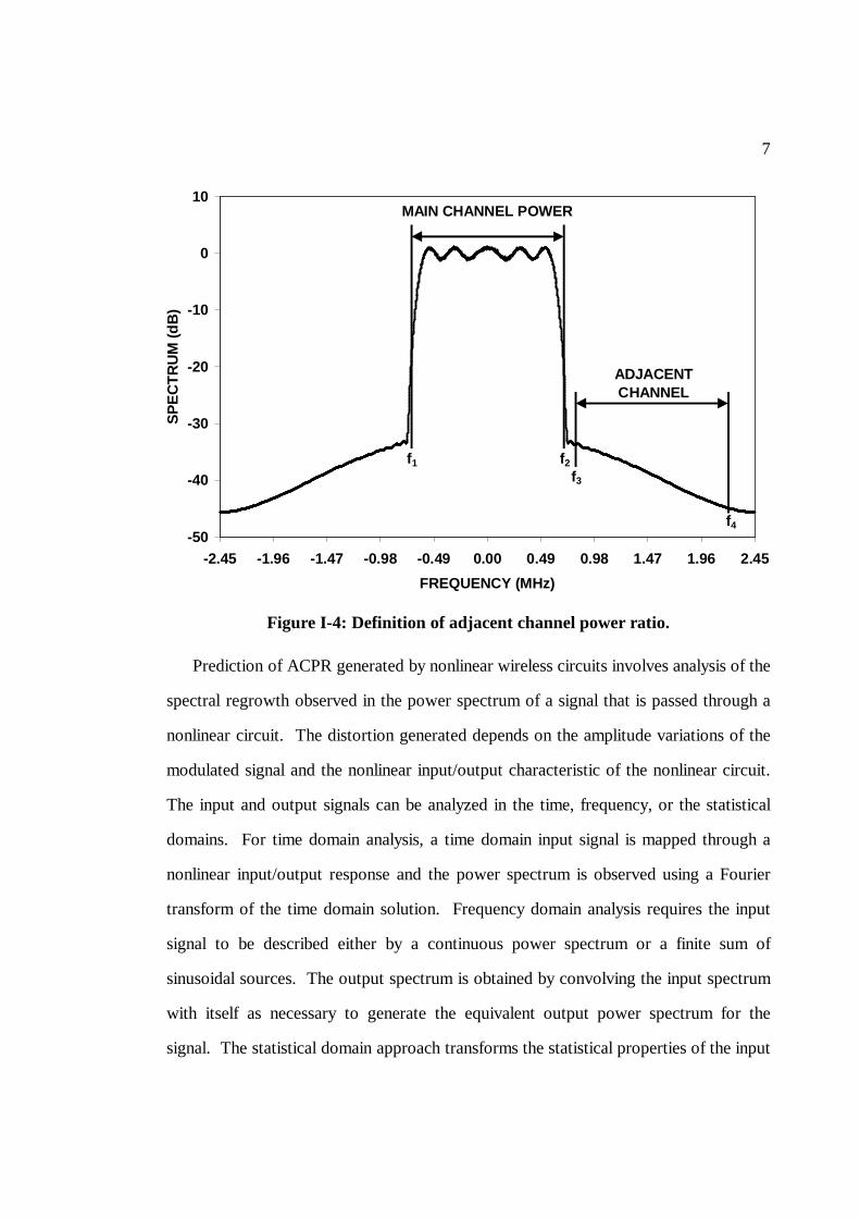
7
Figure I-4: Definition of adjacent channel power ratio.
Prediction of ACPR generated by nonlinear wireless circuits involves analysis of the
spectral regrowth observed in the power spectrum of a signal that is passed through a
nonlinear circuit. The distortion generated depends on the amplitude variations of the
modulated signal and the nonlinear input/output characteristic of the nonlinear circuit.
The input and output signals can be analyzed in the time, frequency, or the statistical
domains. For time domain analysis, a time domain input signal is mapped through a
nonlinear input/output response and the power spectrum is observed using a Fourier
transform of the time domain solution. Frequency domain analysis requires the input
signal to be described either by a continuous power spectrum or a finite sum of
sinusoidal sources. The output spectrum is obtained by convolving the input spectrum
with itself as necessary to generate the equivalent output power spectrum for the
signal. The statistical domain approach transforms the statistical properties of the input
-50
-40
-30
-20
-10
0
10
-2.45 -1.96 -1.47 -0.98 -0.49 0.00 0.49 0.98 1.47 1.96 2.45
FREQUENCY (MHz)
SP
EC
TR
UM
(dB
)
MAIN CHANNEL POWER
ADJACENT CHANNEL
POWER
f3
f4
f1 f2

8
signal through the nonlinearity to yield, or predict, the output statistical properties.
The power spectrum of the transformed statistical signal is obtained through the
Fourier transform of the autocorrelation function of the output signal.
I.2 Wireless Digital Communications
Modern wireless systems employ a variety of digital communication techniques
designed to maximize the number of users that can access the system at any given time.
Two high level systems are used; code division multiple access (CDMA) and time
division multiple access (TDMA). CDMA systems permit multiple users to access the
same frequency simultaneously by using orthogonal coding channels to separate each
user. IS-95, CDMA2000, WCDMA, UMTS, and TD-SCDMA are digital cellular
standards for CDMA systems. TDMA systems permit users to access the channel one
at a time for a short period of time. GSM, DCS, NADC, and Tetra are digital cellular
standards for TDMA systems. Currently both CDMA and TDMA technologies are
used throughout the world. Carriers in the United States use CDMA, TDMA, and
analog FM systems. Carriers in Europe use GSM and the emerging WCDMA system,
while the rest of the world is a mixture of CDMA, WCDMA, and TDMA systems.
However, it should be noted that almost all third generation (3G) systems, including
CDMA2000, WCDMA, and TD-SCDMA, are based upon CDMA.
Both CDMA and TDMA systems use a variety of digital modulation formats. Data
from each digital system is encoded as 1's and 0's, but the encoded information bits
must be imparted on a radio frequency (RF) carrier before the signal can be transmitted
over a wireless channel. Channel bandwidth and signal-to-noise ratio (SNR) are two
important tradeoffs when selecting a modulation scheme to use for a wireless system.
The available bandwidth for any wireless standard is limited by the system design to
maximize capacity at the required data rates.

9
For the purpose of this dissertation, modulation formats are classified as either
constant envelope or non-constant envelope modulation. The envelope is the
amplitude modulation imparted on a radio frequency carrier. Constant envelope
modulation includes frequency shift keying (FSK), frequency modulation (FM),
Gaussian mean shift keying (GMSK), phase shift keying (PSK), and other techniques
involving detection of symbols by frequency or phase shifts of the carrier envelope.
Non-constant envelope modulation includes amplitude modulation (AM), quadrature
phase shift keying (QPSK), offset QPSK (OQPSK), differential QPSK (DQPSK),
quadrature amplitude modulation (QAM), and other techniques involving detection of
variations in envelope amplitude.
Interestingly, amplitude modulation is not inherently required for information
transmission for many modulation schemes with envelope amplitude variation. For
instance, a QPSK signal consists of two digital data streams, equal in amplitude,
modulated in quadrature onto a carrier signal. The resulting signal is constant
envelope; however, the occupied bandwidth is quite large and the first sidelobe of the
sin(x)/x, or sinc, spectrum will only be 13dB down from the carrier in the middle of the
adjacent channel. Typically, a low-pass filter is applied to each digital data stream to
minimize or limit the out of band spectrum of the signal. The filters impart some finite
memory on the data stream which results in amplitude variations as the ringing energy
from a previous data pulse add with the current data pulse.
Amplitude variations of the modulated signal are characterized by measured
waveform statistics. Commonly, the peak to average power ratio (PAR), reported in
decibels, is a popular statistic for describing signals with amplitude variation.
Generally, a signal with higher a PAR require amplifiers with higher linearity to handle
the average power requirements and the peak amplitude excursions without generating
excessive out of band distortion. However, it is possible for a signal with a higher PAR

10
to exhibit less nonlinear distortion than a signal with lower PAR [3]. The reason for
the inconsistency is because the signal peak is a singular point measurement with,
typically, a low probability of occurrence. Thus PAR is an incomplete statistic for
determining the linearity requirements for a transmitter to carry a signal.
The amplitude probability density function (APDF) is a more complete statistical
description of amplitude variations of a modulated signal. The APDF defines the
maximum and minimum variation along with the relative probability of occurrence of
amplitudes within the variation. The APDF is typically estimated from a histogram of
amplitudes, with a uniform bin size, by
cNA
NAf
*)(
∆= (I.2)
where N is the number of counts per bin, ∆A is the bin amplitude width, and Nc is the
total number of samples. The shape of the amplitude density between the mean and
peak amplitude influences the sensitivity of a particular signal to spectral regrowth due
to nonlinear gain compression or expansion. For example, Figure I-5 shows the APDF
for a CDMA mobile transmitter using OQPSK modulation, the same signal using
QPSK modulation, a real Gaussian signal, and a complex Gaussian QPSK signal where
the average power of each signal is set to 0 dBm. The OQPSK signal has the
quadrature data stream offset in time by half the symbol rate while the inphase and
quadrature data for the QPSK signal are clocked together. The real Gaussian signal is
a carrier modulated samples of a Gaussian process passed though the IS-95 reverse link
baseband transmitter filter while the complex Gaussian signal is the quadrature sum of
two independent samples of a filtered Gaussian process. The PAR for each signal is
shown in Table I-2. The shape of the amplitude density after the mean differs for both
signals where a significant portion of the QPSK amplitude above the mean resides close
to the mean while the OQPSK amplitude density is more linear after the mean. Thus it

11
is difficult to determine, a priori, which signal will be more sensitive to nonlinear gain
compression or expansion even though the QPSK has a higher PAR than OQPSK.
The Gaussian signals are interesting because of the difference between the real and
complex Gaussian signals. The complex Gaussian signal is the quadrature sum of two
real Gaussian processes, so an intuitive guess would suggest that the amplitude
distribution should be wider for the complex signal. Exactly the opposite is true; the
POR of the complex Gaussian signal is 1.7 dB less than the real Gaussian signal. An
explanation for this is that the average power of each real Gaussian input signal is
scaled down by 3 dB to yield the correct complex Gaussian power level; however, it is
an unlikely event that two peaks from each of the real Gaussian signals will occur at the
same time leading to a peak signal that is less than 3 dB plus the peak Gaussian
amplitude. Thus the POR is reduced since the peak distributions do not add in power.
Again, from just the POR, it is difficult to determine which signal will yield the least
amount of distortion for the same output power level.

12
-1
0
1
2
3
4
5
6
7
8
9
0.0 0.1 0.2 0.3 0.4 0.5 0.6 0.7 0.8 0.9 1.0 1.1 1.2Envelope Magnitude (V)
Am
plit
ud
e P
rob
abili
ty D
ensi
ty
CDMA OQPSK
CDMA QPSK
Complex Gaussian
Real Gaussian
Figure I-5: Amplitude PDF for CDMA and Gaussian modulation signals.
Table I-2: Decibel peak to average ratio for CDMA and Gaussian signals.
Signal Modulation POR
OQPSK CDMA 5.4
QPSK CDMA 6.6
Real Gaussian 13.5
Complex Gaussian 11.8
I.3 Bandpass Nonlinearities
Bandpass analysis simplifies the formulation of the nonlinear response by separating
the envelope of the modulation from its carrier signal. However, this analysis assumes
that the modulation bandwidth is narrow in comparison to the carrier frequency such

13
that distortion terms from other tones and harmonics related to the carrier do not
overlap in the resulting output spectrum. A carrier signal with amplitude and phase
modulation is expressed as
[ ])(cos)()( tttAtw c θω += (I.3)
where A(t) and θ(t) are the respective amplitude and phase components of the
modulation. The carrier modulation is often referred to as the complex envelope and is
expressed either in polar form
)()()(~ tjetAtz θ= (I.4)
or rectangular form
)()()(~ tjqtitz += (I.5)
where i(t) and q(t) represent the inphase and quadrature components of the baseband
input signal. The modulated carrier expressed in terms of the complex envelope is
.)(~2
1)(~
2
1)( * tjtj cc etzetztw ωω −+= (I.6)
The concept of bandpass nonlinearities was developed in the 1950s by information
theorists who needed a simple model of a nonlinear channel to analyze the degradation
in C/N of a modulated RF carrier passed through a nonlinear circuit followed by a
bandpass filter centered at the carrier frequency [4]. The output bandpass filter
eliminated all other distortion components except those centered about the carrier
frequency. The resulting analysis is simplified by eliminating the need to consider other
nonlinear terms harmonically related to the carrier frequency. Various behavioral
models for the nonlinearities are used including power series [5], Chebyshev
transformations [6, 7], and Bessel function expansions [8].

14
The simplest characterization of a bandpass nonlinear circuit is by its instantaneous,
or memoryless, large signal input output response. For a modulated carrier this
requires sweeping the input amplitude of an unmodulated carrier and measuring the
corresponding change in gain and phase at the output port of the circuit. The
amplitude gain response is known as the amplitude modulation to amplitude
modulation transfer characteristic (AM-AM) and the amplitude phase response is the
amplitude modulation to phase modulation (AM-PM) characteristic. The bandpass
nonlinear response in terms of the complex envelope is
[ ] [ ] [ ] )()()()(~~ tAtjetAFtzG Φ+= θ (I.7)
where [ ]( )F A t and [ ]( )A tΦ are the AM-AM and AM-PM response functions
respectively. Once the AM-AM and AM-PM response is obtained either by
measurement or simulation, the data can be used directly with a numerical interpolation
routine or used to fit model parameters to best fit the model to the data.
The power of the AM-AM and AM-PM representation is the ease of extraction of
the characteristic and simplification of nonlinear analysis. The input/output
characteristic is measured by sweeping the input power or signal level and measuring
the resulting gain and phase at the output using a vector network analyzer or vector
voltmeter relative to a fixed reference signal. Likewise the characteristic can be
simulated using a SPICE transient, steady-state shooting method, or harmonic balance
circuit simulation engine to simulate the steady-state gain and phase transfer function as
the input signal is swept in power. The negative tradeoff of using a memoryless
nonlinear model is that frequency dependencies in the linear and nonlinear response are
not modeled resulting in modeling errors for devices with strong frequency variation
over the modulation bandwidth or over the bandwidth of distortion terms which
contribute significantly to the output spectrum.

15
I.4 Power Spectrum Estimation
Engineers routinely use fast Fourier transform (FFT) or discrete Fourier transform
(DFT) to estimate the power spectrum of signals. A Fourier transform is performed on
the resulting output complex envelope signal to obtain the output power spectrum [9]
2
2( ) ( ) .j ftS f z t e dtπ∞
−∞
= ∫ ɶ (I.8)
where f is frequency. This approach is known as the direct method of spectral
estimation of the output power spectrum. While this method is straightforward in its
application, it provides little insight into how the nonlinear model and signal interact
together to produce the output spectrum. At best, different parameters can be altered,
extract a new model, run the signal through the model, observer the resulting spectrum,
and deduce the sensitivities.
The indirect method is an alternative approach to calculate the power spectrum by
first calculating the autocorrelation function of the signal at the output of the model
then compute the Fourier transform of the autocorrelation function. The
autocorrelation function is the convolution of a signal with its complex conjugate
∫∞∞−
+= .)(~)(~)(~ * dttztzR ττ (I.9)
Once the autocorrelation function is calculated the power spectrum is estimated from
the Weiner-Khinchine theorem [10]
∫∞∞−
= .)(~
)(~ ττ ωτ deRfS j (I.10)
where 2 fω π= . If )(~ tz is a series expansion, then the autocorrelation function is a
summation of products of all combinations of terms in the series, and the resulting

16
power spectrum is a summation of individual spectra from the Fourier transform of
each term in the series. Thus if the terms of the series expansion of the autocorrelation
function have physical meaning to the nonlinear circuit then the power spectrum is
expressed in terms of a summation of products of those terms. This provides insight
into how parameters in the nonlinear model interact with the signal to affect changes in
the resulting power spectrum.
I.5 Spectral Regrowth Analysis
Analysis of spectral regrowth generated by nonlinear wireless circuits involves
finding the solution for the output power spectrum of a modulated signal that is passed
through a nonlinear circuit. Direct simulation solutions to the problem are difficult to
obtain due to the large number of active devices found in modern wireless integrated
circuits and the number of simulation points needed to resolve the power spectrum of a
modulated high frequency carrier signal. This section presents an overview of the
simulation and behavioral modeling techniques available for assessing the spectral
regrowth generated by a nonlinear wireless circuit when processing a high frequency
modulated carrier.
Estimation of spectral regrowth and intermodulation distortion has been
approached in a variety of ways. Recently, De Carvalho and Pedro [11] analyzed the
excitation of a nonlinear circuit by a large number of input tones based on the spectral
balance method, and used the resulting algorithm to predict ACPR and Noise-Power
Ratio (NPR). A number of rapid system-level methods have been proposed to
characterize spectral leakage to adjacent channels. Sevic, Steer, and Pavio [12] used
least squares fitting of a power series to AM-AM and AM-PM transfer data to predict
amplitude and phase transformation through nonlinear microwave power transistors. It
was found that ACPR can loosely correlate to the third order intermodulation product
(IP3), although the presence of strong fifth-order nonlinearity, either due to loading or

17
intrinsic device characteristics, can impact ACPR in the Japanese TDMA digital
system. Chen, Panton and Gilmore [13] developed a method to predict ACPR and
NPR based on a time domain analysis technique and bandpass nonlinearity theory. AM-
AM and AM-PM transfer characteristics are used to directly predict samples of the
output complex envelope based on samples of an input complex envelope and the
algebraic expression for a bandpass nonlinearity given by the describing function and
corresponding nonlinear phase and amplitude.
I.5.1 Transient Analysis of Spectral Regrowth
Robust time step integration algorithms from SPICE based simulators have made
transient simulators ubiquitous with modern integrated circuit design. However,
simulation of wireless digital communication signals require small time steps to
accurately capture the RF carrier and a long simulation period to resolve multiple
symbols of the modulation. To make matters worse, time step integration methods
found in typical SPICE [14] simulators require the minimum time step size to be ten to
twenty times smaller than the period of the highest frequency source in the circuit in
order to accurately resolve a sinusoidal signal. The approximate number of transient
time steps required is
RSBW
fN tstep
max10×≈ (I.11)
where fmax is the maximum frequency source in the circuit and RSBW is the desired
resolution bandwidth needed to resolve the spectrum of the modulation. For example,
transient simulation of a 2 GHz carrier frequency with 1 kHz resolution requires a
minimum 25 psec time step and 1 msec simulation duration time resulting in a solution
of forty million time points. Transient simulation of a RFIC signal path of moderate
complexity would require a week or more of CPU time to complete the simulation. An

18
example plot of a transient simulation output of modulated carrier waveform versus
time is shown in Figure I-6.
Time
Am
plit
ude
Figure I-6: Transient simulation of modulated carrier.
I.5.2 Harmonic Balance Analysis of Spectral Regrowth
Harmonic balance simulators find the large signal steady-state solution of circuits in
the frequency domain using Fourier coefficients to represent current and voltage signals
[15]. The circuit netlist is partitioned into two groups; one containing the linear
frequency domain components and the other group containing all of the quasi-static
nonlinear components as is shown in Figure I-7. The solution for the linear portion of
the circuit is a straightforward linear matrix solution for each of the frequency domain
state variables. A direct frequency domain solution of the nonlinear circuit is requires a
complicated Fourier decomposition of each nonlinear equation and a convolution of
spectral tones and harmonics of sources applied to the circuit. Instead, the nonlinear

19
solution is handled indirectly by performing an inverse Fourier transform of the Fourier
coefficients at the boundaries of the linear and nonlinear circuits to generate a time
domain waveforms which are then applied to the nonlinear time domain equations and a
Fourier transform is performed on the resulting waveforms. Simulation ends when the
error between the Fourier coefficient state variables of the linear and nonlinear circuits
reduces to an acceptable tolerance. Formulation of the harmonic balance solution
begins with a steady state time domain solution to Kirchhoff’s current law (KCL) [16,
17]
( ) ( ) ( )( ) ∫∞−
=+−++=t
tudvtytvqitvittvf 0)()()()()(),( τττɺ (I.12)
where ( )( ),f v t t is the formulation of KCL used in a Newton iteration scheme and
circuit currents are expressed in terms of conductance, voltage dependent charge, linear
dispersive, and input sources. The KCL equation transformed to the frequency domain
is
( ) 0)()( =++Ω+= UYVVQVIVF (I.13)
where the time derivative of charge is transformed to 2j fπΩ = and the convolution of
the linear circuit is a product of AC admittance and voltage.

20
LinearCircuit
Elements
NonlinearCircuit
Elements
FFT
)(~1 ωV
)(~
2 ωV
)(~
3 ωV
)(~
4 ωV
)(~ ωNV
)(1 tv
)(1 ti
)(2 tv
)(2 ti
)(3 tv
)(3 ti
)(4 tv
)(4 ti
)(tvN
)(tiN
)(~1 ωI
)(~
2 ωI
)(~
3 ωI
)(~
4 ωI
)(~ ωNI
IFFT
Figure I-7: Circuit partitioning for harmonic balance analysis.
The difficulty of simulating digital modulated waveforms with harmonic balance
arises from describing the modulation as a finite set of Fourier coefficients. It is
possible to describe a time-domain waveform as a set of Fourier coefficients [18];
however, the memory demands and computational complexity of the harmonic balance
analysis grow on order 3N with the total number of state variables needed in the
solution. The computational demands are a result of the Newton-Raphson iteration
scheme used to iteratively solve the nonlinear system of equations. The formulation
requires inversion of a Jacobian matrix containing time derivatives of the state
variables. Iterative approximation techniques have been applied to solving the Newton-
Raphson iteration step using Krylov subspace techniques resulting in a reduction of
computational complexity to less than order 2N and reduced memory requirements
[19]. Harmonic balance simulation has been demonstrated on large nonlinear circuits
with sinusoidal modulation [20] and on small circuits with Fourier coefficients of

21
digitally modulated waveforms [21, 22]; however, harmonic balance simulation of large
RFIC circuits with digital modulated waveforms applied is not yet practical.
I.5.3 Envelope Simulation of Spectral Regrowth
Envelope simulation techniques are based upon the premise that the modulated
envelope of the high frequency carrier is changing slowly in time relative to the carrier
such that the envelope solution can be solved as a sequence of steady state solutions,
either from harmonic balance or time domain shooting methods, of the carrier stepped
in time [23-25]. Envelope simulation is also referred to as mixed time/frequency
simulation because the solution of the carrier is a sinusoidal steady state frequency
domain solution and the envelope is a time domain solution. In a sense, envelope
simulation is an example of bandpass sampling solution of the envelope about the
carrier frequency. Formulation of the envelope solution starts with a time variant
version of the frequency domain KCL equation [24]
( ) ( ) ( ) ( )( )( ), ( ) ( ) ( ) 0
dQ V tF V t t Q V t I V t U t
dt= + Ω + + =
ɶ ɶ ɶɶ ɶ ɶ ɶ ɶ ɶ (I.14)
where the extra time varying charge term comes from the envelope ( )V tɶ and Ω is a
diagonal matrix with 2j kfπ on the thk diagonal. Differentiation of the envelope charge
term can be approximated with a finite difference formulation such as backwards Euler
method
( ) ( ) ( ) ( ) ( )1
1
( ) ( )( ), ( ) ( ) ( ) 0 .
m m
m m mm m
Q V t Q V tF V t t Q V t I V t U t
t t
−
−
−= + Ω + + =
−
ɶ ɶɶ ɶ ɶɶ ɶ ɶ ɶ ɶ ɶ (I.15)
Harmonic balance frequency domain models can be used for the carrier steady state
response; however, additional time domain descriptions for each component are
required for the transient envelope solution. Recently, time domain steady-state

22
Newton shooting methods [26, 27] have been applied to commercial transient envelope
simulators [23, 28].
The required number of samples of the envelope depends on the input signal length,
desired resolution bandwidth, and the simulator accuracy and time step control
parameters. Thus the number of simulation points is greatly reduced over the transient
and harmonic balance solutions since the solution requires approximately
RSBW
BWN ≈ (I.16)
steady-state solutions of the carrier signal where BW is the bandwidth the signal and
the spectral regrowth. Compared to the earlier transient example, envelope simulation
requires 10,000 single carrier solutions to provide 1 kHz resolution of a signal
spectrum with 10 MHz bandwidth. An example plot showing the sampled envelope
and steady-state carrier solutions versus time are shown in Figure I-8. For the special
case of two tone modulation, the RSBW can be set to the tone spacing and the BW to
ten to twenty times the RSBW to capture the resulting intermodulation distortion
spectrum thus the number of required steady-state solutions of the carrier is reduced to
ten or twenty. However, for wide bandwidth digital modulated signals the required
number of samples increase linearly with the bandwidth for a fixed RSBW.
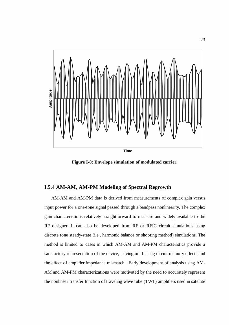
23
Time
Am
plit
ude
Figure I-8: Envelope simulation of modulated carrier.
I.5.4 AM-AM, AM-PM Modeling of Spectral Regrowth
AM-AM and AM-PM data is derived from measurements of complex gain versus
input power for a one-tone signal passed through a bandpass nonlinearity. The complex
gain characteristic is relatively straightforward to measure and widely available to the
RF designer. It can also be developed from RF or RFIC circuit simulations using
discrete tone steady-state (i.e., harmonic balance or shooting method) simulations. The
method is limited to cases in which AM-AM and AM-PM characteristics provide a
satisfactory representation of the device, leaving out biasing circuit memory effects and
the effect of amplifier impedance mismatch. Early development of analysis using AM-
AM and AM-PM characterizations were motivated by the need to accurately represent
the nonlinear transfer function of traveling wave tube (TWT) amplifiers used in satellite

24
communication systems. Kaye [7] formulated the complex gain as a quadrature sum of
two independent memoryless nonlinearities, modeled as Chebyshev transforms, to
account for AM-PM effects. Previous analysis was either based on analytical models
not derived from measurements [8] or on AM-AM characterization only.
Many early models used Chebyshev or Bessel series expansions as behavioral
models of the channel nonlinearity because the formulations included integrals of
sinusoids with functions of time included in the argument. Koch [29] proposed using a
Taylor series expansion of a nonlinear AM-AM transfer function to calculate distortion
generated when a white noise signal is passed through a memoryless nonlinearity.
Later Kuo [30] proposed improvements and corrections to the Taylor series derivation;
although, the analysis was still limited to AM-AM only nonlinearity. Hieter [31] added
independent time delays to each nonlinear variable in a power series expansion to
account for AM-PM effects. Steer and Kahn [32] generalized the power series
representation by adding complex coefficients. Later the generalized power series
analysis (GPSA) approach was applied to a variety of microwave device modeling and
simulation problems including MESFET amplifiers [5], bivariate power series modeling
of amplifiers [33], and spectral balance simulation techniques [34, 35].
Lajoinie et al. [36] developed a modification of the method described by Chen et
al. [13] that extends it to the prediction of NPR in amplifiers exhibiting nonlinear low
frequency dispersion (memory effects) such as satellite transponders. Sevic and
Staudinger [37] presented a comparison of the behavioral model approach and a
commercial, envelope simulation technique. The envelope simulation technique does
take into account nonlinear circuit memory effects, but has the disadvantages of
requiring accurate circuit component models and prohibitive simulation run time.

25
I.5.5 Volterra Series Modeling of Spectral Regrowth
Volterra series provides the most general form of analytical analysis of nonlinear
circuits; however, it is typically a laborious process to derive a formulation even for the
simplest of circuits. Nevertheless, it is a useful analysis technique for assessing spectral
regrowth and has received more attention in the recent literature. Leke and Kenney
[38] generated analytical expressions for gain compression and phase distortion from a
third-order Volterra nonlinear transfer function model and used these to predict
spectral regrowth of a MESFET power amplifier. Their method presents a connection
between intermodulation distortion and spectral regrowth, but is limited by the
increasing complexity of the Volterra analysis for transfer functions above third order.
Maas [39] represented the modulated input signal as a sum of sinusoids and applied
third order Volterra analysis to find all third order terms that end up about the carrier
frequency. A commercial Volterra software package was used to simulate the resulting
spectral regrowth generated about the carrier; however, the results were not compared
to measurement or theoretical data to determine limitations of the analysis or the
number of sinusoids needed to accurately represent the modulated input signal. Van
Moer [40] showed spectral regrowth analysis from Volterra kernel models extracted
from continuous wave (CW) measurements of microwave nonlinear circuits. Garcia
[41] used time-varying Volterra series to analysis spectral regrowth distortion
generated by a microwave mixer circuit showing that a large number of tones could be
efficiently used with Volterra analysis to solve for the spectral regrowth. Recently
Aparin [42] derived an analytical expression for crossmodulation distortion spectrum
generated between a continuous wave (CW) jammer and OQPSK transmitter signals
present at the input of a CDMA low noise amplifier (LNA) from Volterra series
analysis of the LNA and an assumption that the baseband modulation was filtered by an
ideal brick wall filter.
26
I.5.6 Statistical Analysis of Spectral Regrowth
While it is widely acknowledged that sideband regrowth depends on the encoding
method (i.e., the statistics of the input stream), little work has been done to estimate
output spectrum as the nonlinear transformation of an input random process. An early
work in communication theory by Baum [43] revealed the general property of spectral
regrowth when a Gaussian signal is passed through a limiting amplifier model. A later
paper investigated the resulting output autocorrelation function of a real Gaussian
variable passed through ideal limiters and power law nonlinearities [44]. Shimbo [8]
developed a general formula for intermodulation for the case where arbitrary
modulated carriers and Gaussian noise are amplified through a TWT system.
Simplified expressions for certain types of nonlinearities one being a power series
model were also presented; although the nonlinear transformation of input signal
moments were not discussed. A landmark publication by Bedrosian and Rice [45]
considered the case of nonlinear systems with memory, and developed expressions for
the Volterra transfer functions (Fourier transforms of the Volterra kernels) when the
system equations are known and the system can be represented by a Volterra series.
Output spectrum estimates are computed for two cases: when the input is zero-mean
stationary Gaussian noise with known power spectrum, and when the input is a sine
wave plus zero-mean stationary Gaussian noise. Formulas for the output probability
density function are also outlined, as they can be obtained by solving certain integral
equations. Rudko and Weiner [46, 47] derived the general output autocorrelation and
power spectrum for Gaussian inputs to a Volterra series representation of a nonlinear
system.
Recently, Wu et al. [48, 49] formulated a relationship between ACPR, IP3 and IP5
based on the output autocorrelation function of a real Gaussian random variable passed
through an AM-AM nonlinear amplifier model. Their approach, however, is limited by

27
several assumptions in the model and derivation. First, the authors use an AM-AM only
model asserting that AM-PM effects cannot be represented by a Taylor series
expansion. However, a complex Taylor series expansion can account for both AM-AM
and AM-PM effects of a memoryless nonlinearity [31, 50, 51]. IP3 specifications are
typically available for amplifiers, but IP5 and higher order terms are not. Thus a
designer must make IP5 measurements to obtain better accuracy in the ACPR estimate
using the method described in [49]. Moreover, both AM-AM and AM-PM effects are
easily extracted from single tone complex gain measurements swept over input power
[31]. Second, their derivation represents the CDMA waveform as a single real
Gaussian random variable when the modulation signal is actually a complex sum of two
random variables (the I and Q data channels). Third, the authors assume the power
spectrum is flat over the modulation bandwidth when the actual signal spectrum shape
is determined by a specific baseband filter response defined by the IS-95 CDMA
standard [2]. Gutierrez, Gard, and Steer [52] have addressed most of these limitations
by developing a closed from expression for the autocorrelation of the amplifier output
based on a moment theorem for complex Gaussian processes and an nth order complex
power series model of the nonlinear amplifier. The output power spectrum is
calculated from the Fourier transform of the output autocorrelation expression in terms
of the input signal autocorrelation and thus does not make assumptions about the shape
of the resulting output power spectrum. This allows convenient evaluation of the
output spectrum for a variety of modulation formats by using estimates of the input
autocorrelation function of each modulation format.
I.5.7 Summary
The previous sections reviewed the current state of the art for simulation,
behavioral modeling, and analytical analysis of spectral regrowth generated by
nonlinear wireless circuits. Circuit simulators struggle with efficiently resolving the

28
modulation about a high-frequency carrier. SPICE-based transient simulators are the
least efficient method due to the simultaneous requirements of a time step small enough
to resolve the carrier frequency with a simulation duration long enough to provide
adequate resolution of the modulation. Harmonic balance solutions struggle with
numerical complexity proportional to the number of Fourier coefficients of modulated
carrier signal and the number of components in the circuit. Envelope transient methods
efficiently solve the resolution versus bandwidth problem by using a sequence of single
carrier steady state solutions to sample the time varying envelope of the carrier;
however, simulation times are still too long to capture a frame or more of typical
modulation data with large RFIC circuit designs. Moreover, each of the time domain
methods require additional processing time to post-process simulation data using a
numerical Fourier transform in conjunction with a power spectrum estimation
technique to analyze the ACPR performance for each power point simulated.
Behavioral models and analytical solutions provide quick solutions for accessing the
effects of spectral regrowth; however, models are limited by the accuracy of the model
and scope of the data used to extract the model. Analytical solutions depend, in part,
on behavioral models to facilitate the analysis, and, in general, are specific to particular
application the problem is derived from. Also, the difficulty and complexity of deriving
analytical solutions is proportional to the level of detail of both the model used and the
analytic description of the modulation.
Statistical analysis of spectral regrowth requires knowledge of the statistical
properties of the modulation signal. Gaussian signals have well known statistical
properties and some relevance to particular problems such as narrow band Gaussian
noise (NBGN) analysis, multicarrier CDMA, and narrow band multicarrier systems.
Unfortunately, the statistical properties of many useful signals are not known for high

29
order problems. A comparison of the relative properties of the different methods for
analyzing spectral regrowth is provided in Table I-3.
Table I-3: Comparison of methods to analyze spectral regrowth.
Method Numerical Complexity Formulation Difficulty
Transient Highest Low
Harmonic Balance High Low
Envelope Moderate Medium
Analytical Low High
Statistical Low High
I.6 Dissertation Organization
The focus of this dissertation is to present an analysis technique for the solution of
the output power spectrum of a modulated signal passed through a nonlinear wireless
circuit. The solution provides potential insight into how the nonlinear circuit and the
signal interact to produce spectral regrowth. In addition, the analysis separates the
output spectrum into individual components of the model and input signal such that the
spectrum is separated into logical contributions to distortion and gain compression or
expansion of the desired signal. Separation of the spectral terms also permits analysis
of inband distortion that contributes to degradation of system SNR due to cochannel
distortion.
Chapter I presents an overview of the ACPR problem in modern wireless
communication systems with a particular example of a CDMA mobile station. A
review of time domain, frequency domain, behavioral model, and analytical techniques
for analyzing spectral regrowth from nonlinear wireless circuits is presented.

30
Chapter II investigates autocorrelation analysis derived from a bandpass
nonlinearity model of the AM-AM and AM-PM characteristic of a nonlinear circuit. A
complex power series expansion is used as a behavioral model of the nonlinear
input/output characteristic to facilitate autocorrelation analysis of the output signal. A
binomial expansion of the nonlinearity is used to select just components of the output
which are centered about the carrier frequency. The autocorrelation of the output
signal, about the carrier, is formulated using the result of the binomial expansion. The
resulting power spectrum of the signal is computed from the Fourier transform of the
autocorrelation function.
Chapter III uses the statistical properties of the input signal to compute the output
autocorrelation function of a wireless nonlinear circuit. Relationships between the time
and statistical averages of random processes are investigated. The time and statistical
averages are equivalent for ergodic stationary signals. The statistical averages or
moments are substituted for the special cases of real and complex Gaussian random
processes. The output autocorrelation function is shown to reduce the complexity of
the formulation of the output autocorrelation function and resulting power spectrum
calculation.
Chapter IV compares transient envelope simulation results with calculated ACPR
for several limiter amplifier models. Two techniques for measuring the AM-AM and
AM-PM characteristics of amplifier and transmitter integrated circuits are presented.
In addition, measured and calculated ACPR data for a CDMA RFIC transmitter
amplifier are compared. Measurements and calculations for the special case of a
complex Gaussian signal are also presented. Both the general autocorrelation and the
statistical autocorrelation results are compared for the complex Gaussian signal.
Chapter V concludes the dissertation with a summary of the presented analysis
techniques and the advantages and disadvantages of the behavioral techniques used to

31
analyze the distortion of wireless integrated circuits. Future areas of work are
discussed as a followup to both the behavioral models approaches and the analysis
techniques presented in this thesis.

32
II. Autocorrelation Analysis of Bandpass Nonlinearities
Analysis of spectral regrowth involves spectral analysis of a signal that has been
passed through a nonlinear channel. The nonlinear channel is represented by a
behavioral model based upon measurement data, simulation data, analytical models, or
look up table models. The simplest analysis involves passing a signal through the
model and observing the spectrum at the output using a fast Fourier transform (FFT);
however, this analysis does not provide insight into how components of the nonlinear
model interact with the signal to generate the observed distortion and gain compression
or expansion characteristics. To gain additional insight requires an analysis technique
that describes the resulting power spectrum in terms of elements of the underlying
nonlinear process, such that relationships between characteristics of the output
spectrum and the model parameters can be determined.
The power spectrum of an output signal can be obtained by either taking the
magnitude squared of the Fourier transformation of the output signal or by first
computing the autocorrelation of the output signal then take the Fourier transformation
of the autocorrelation function. Many engineers simply elect to take the Fourier
transform of the output signal; however, there are benefits to exploring the
autocorrelation approach to obtain the power spectrum. The autocorrelation function
of the output signal involves taking the convolution of the output signal with a time
shifted version of the complex complement of the output signal. The resulting
formulation contains a summation of power terms that are described by the nonlinear
model and individual autocorrelation terms. Finally the Fourier transformation of each
of the terms is taken and summed to describe the output power spectrum. The
resulting power spectrum can be investigated in a variety of ways by singling out
individual terms, groups of relevant terms such as gain compression/expansion or

33
distortion terms, or summed together to view the complete output power spectrum.
Such flexibility provides a means to gain additional insight into the relationship between
the nonlinear model and the distortion products generated when a nonlinear circuit or
system component is modulated waveform with amplitude variation.
Irregardless of the spectral analysis method used, a behavioral model of the
nonlinear circuit or system component must be selected to assist the analysis. There
are many models to choose from; however, a power series representation is one of the
simplest models to deal with when working with analytical expressions involving
signals and nonlinearities. The simplicity of the model adds clarity to the signal analysis
techniques presented in this and the following chapter; moreover, the analysis presented
can always be expanded to more complicated models including Volterra series
descriptions.
This chapter presents an overview of bandpass nonlinearity analysis of a modulated
carrier signal passed through a complex power series behavioral model of a nonlinear
wireless circuit. The bandpass nonlinearity analysis yields a description of the transfer
function of the input signal to the first harmonic response of the nonlinear circuit. An
autocorrelation analysis of the output of the nonlinear model is formulated and a
Fourier transform performed to yield the output power spectrum in terms of the power
series model and correlation terms of the input signal. Power sweeps of the input
signal are performed with power series representations of several different analytical
limiting amplifier models and the power spectrum and ACPR are measured at the
output versus the output power. The results are compared to transient envelope
simulation results using the analytical limiter models.
II.1 Bandpass Nonlinearity Analysis
A wireless digital communication signal is generated from a quadrature modulator
as shown in Figure II-1. Inphase and quadrature carrier signals are mixed respectively

34
with two analog input signals representing the inphase and quadrature symbol
components of the data. The mixed signals are summed together to form the
quadrature modulated carrier signal.
NONLINEAR DEVICEQUADRATURE MODULATOR
90°
( )i t
( )q t
cos( )ctωΣ
( )w tGɶ [ ]( )G w tɶ
cω
[ ]( ) c
c
j tG z t e ωω
ɶ ɶBANDPASS OUTPUT
Figure II-1: Block diagram of quadrature modulator and bandpass nonlinearity.
Consider the complex envelope representation of an amplitude and phase modulated
carrier, w(t), with carrier frequency fc,
*
( ) ( ) cos[ ( )]
1 1( ) ( )
2 2c c
c
j t j t
w t A t t t
z t e z t eω ω
ω θ−
= +
= +ɶ ɶ
where
2 2
1
( ) ( ) ( ) ,
( ) ( ) ( ) ,
( )( ) tan ,
( )
z t i t jq t
A t i t q t
q tt
i tθ −
= +
= + = ɶ
( )z tɶ is the complex envelope, i(t) and q(t) are the inphase the quadrature components
of the baseband modulation respectively, and 2c cfω π= . The concept of complex
envelope representation of narrow band signals was presented early in the development
of the information theory [53, 54].

35
The modulated carrier signal is applied to a nonlinear circuit with a nonlinear gain
characteristic, [ ])(~
twG . The nonlinear gain characteristic is assumed to be a bandpass
nonlinearity containing no significant memory within the bandwidth of the modulation
[4]. Thus, the AM-AM and AM-PM nonlinearities respond instantaneously to
amplitude changes from the modulated carrier signal. It is important to note that the
AM-AM and AM-PM response represents the transfer characteristic of the input to the
desired output frequency. A complex power series expansion is used to model the
instantaneous AM-AM and AM-PM characteristics
[ ] 3 5
1 3 5
( 1) /22 1
2 10
( ) ( ) ( ) ( ) ( )
( ).
NN
Nn
nn
G w t a w t a w t a w t a w t
a w t−
++
=
= + + + +
= ∑ɶ ɶ ɶ ɶ ɶ…ɶ (II.1)
The use of complex coefficients in the power series provides the necessary degrees of
freedom to represent both the AM-AM and AM-PM properties of a nonlinear gain
characteristic [32].
In general, the power series contains all powers of the input signal; however, only
the odd order terms generate output components at the fundamental frequency. To see
why this is, consider the case where the input single is an unmodulated carrier signal
( ) cos( )cw t A tω= (II.2)
and the second order term of a power series is
[ ]
2 2 2
2
( ) cos ( )
1 cos(2 )2
c
c
w t A t
At
ω
ω
=
= + (II.3)

36
thus even order terms generate components at baseband and at even order harmonics of
the carrier frequency. Now consider the first even order term, above the fundamental,
of the power series
[ ]
3 3 3
3
3 3
( ) cos ( )
1 cos(2 ) cos( )2
3cos( ) cos(3 )
4 4
c
c c
c c
w t A t
At t
A At t
ω
ω ω
ω ω
=
= +
= +
(II.4)
thus even order series terms generate components at the fundamental and at odd order
harmonics of the carrier frequency. Therefore only an odd order series, or function,
can describe the nonlinear transfer function of an input carrier signal to the output
components which end up at the carrier frequency.
To simplify the analysis, a binomial expansion is used to compute the mth power of
w(t) yielding [50, 55]
[ ] [ ] .)(~)(~2
1)( )2(*
0
tmkjkmkm
km
m cetztzk
mtw −−
=∑ = ω (II.5)
Consider now only the terms centered at the carrier frequency (this is usually
referred to as the first zonal filter output of the nonlinearity). This implies 2 1k m− = ±
for odd m only. Substituting ( 1) / 2k m= + , the terms of (II.5) around the carrier
frequency are
[ ]11
* 221
1( ) ( ) ( ) .1
22
c
c
mmj tm
m
mw t z t z t em
ωω
−+±
−
= + ɶ ɶ (II.6)
It is convenient to rewrite (II.6) in terms of a sequence of odd powers by substituting
m=2n+1

37
[ ] 12 1 *2
2 11( ) ( ) ( ) .
12c
c
nn j tnn
nw t z t z t e
nω
ω+ ±+ + = + ɶ ɶ (II.7)
Now the transfer function of the fundamental response can be written as
[ ]( 1) / 2
2 12 1
0
( ) ( ) .c
c c
Nj tn
nn
G w t a w t e ωω ω
−±+
+=
= ∑ɶ ɶ (II.8)
The fundamental response can also be defined as a function of the complex envelope
[ ] [ ]( ) ( ) c
c c
j tG w t G z t e ωω ω
±=ɶ ɶ ɶ (II.9)
where
[ ]1
21 *2 1
20
2 1( ) ( ) ( ) .
12c
N
nnnn
n
naG z t z t z t
nω
−
++
=
+ = + ∑ ɶɶ ɶ ɶ ɶ (II.10)
This expression describes the complex envelope of the first harmonic of a modulated
carrier signal passed through a bandpass nonlinear circuit described by a complex
power series.
So far the analysis assumes that the complex power series coefficients are obtained
directly from the underlying nonlinear function. The binomial and 21/ 2 n terms from
(II.10) account for the effect of a sinusoidal carrier signal being passed through a
power series representation of a nonlinear function. Effectively these coefficients
provide a describing function representation of the nonlinearity when the underlying
nonlinear function is known [56]. Describing functions are used in control theory to
simplify the analysis of a nonlinear block with feedback by just considering the
fundamental response of a memoryless nonlinearity when a sinusoidal input is applied.
The AM-AM and AM-PM characteristic also is a describing function representation of
the underlying nonlinearity. Typically it is straightforward to obtain the carrier gain

38
characteristic directly either by simulation or measurement. For this case, the carrier
effects are already included in the measurement data in which case the complex
envelope expression (II.10) can be restated as
[ ]1
21 *
2 10
( ) ( ) ( )c
N
nnn
n
G z t b z t z tω
−
++
=
= ∑ ɶɶ ɶ ɶ ɶ (II.11)
where
2 12 1 2
2 1.
12n
n n
nab
n+
+
+ = + ɶɶ
The 2 1nb +ɶ coefficients can be obtained from a least squares fit of the measured or
simulated carrier transfer function.
II.2 Autocorrelation Analysis of Spectral Regrowth
Many engineers tend to think of the power spectrum as the magnitude squared of
the power spectrum because of its simplicity and easy of computation; however,
fundamentally the power spectrum is related to the time domain signal via the
autocorrelation function. Therefore it is worthwhile to understand the relationship
between the autocorrelation function, the time domain signals it represents, and the
power spectrum of the signal. Starting with a band limited time domain signal
( )z tɶ (II.12)
the power spectrum of the signal is
2
*
( ) ( )
( ) ( )
S f Z f
Z f Z f
=
=
ɶ ɶɶ ɶ (II.13)

39
where * denotes the complex conjugate of the signal and ( )X f is the Fourier
transform of ( )z tɶ
2( ) ( ) .j ftZ f z t e dtπ∞
−
−∞
= ∫ɶ ɶ (II.14)
One useful property of Fourier transform pairs is multiplication in the frequency domain
is convolution in the time domain
* *( ) ( ) ( ) ( ) .j fZ f Z f e df z t z t dtωτ τ∞ ∞
−∞ −∞
= −∫ ∫ɶ ɶ ɶ ɶ (II.15)
Now define the autocorrelation function of ( )z tɶ to be
*( ) ( ) ( )zz z t z t dtτ τ∞
−∞
ℜ = −∫ɶ ɶ ɶ (II.16)
where the subscript zz indicates what signals the autocorrelation is operating on. The
power spectrum is the Fourier transform of the autocorrelation function according to
the Wiener-Khinchine relation [57-59]
* 2
2
( ) ( ) ( )
( ) .
j f
j fzz
S f z t z t e dtd
e d
π τ
π τ
τ τ
τ τ
∞ ∞−
−∞ −∞∞
−
−∞
= −
= ℜ
∫ ∫∫ɶ ɶ (II.17)
Use of the autocorrelation function has the advantage of providing a method to
compute each component of the output spectrum in terms of the input signal and the
nonlinear model. The time average autocorrelation function of ( )z tɶ , ( )zz τℜɶ , is defined
as the convolution of a signal with its complex conjugate [60, 61]

40
.)(~)(~2
1lim)(
~ *∫−
∞→+=ℜ
T
TT
zz dttztzT
ττ (II.18)
Later in this dissertation, the statistical autocorrelation function, defined by an
expectation operator, will be discussed as an alternative to the time average
autocorrelation function when the statistical moment properties of the signal are
known. The time average autocorrelation function can be applied to a realization of a
time domain signal; however, it can not, in general, be assumed that the time average
autocorrelation function represents the statistical average of all realizations of a signal.
A common property of all autocorrelation functions is
*( ) ( )zz zzτ τℜ = ℜ −ɶ ɶ (II.19)
thus the real part of autocorrelation function is an even function while the imaginary
part is odd. The autocorrelation function is related directly to the power of the signal
when 0τ =
21lim ( )
2
(0) .
T
zT
T
zz
P z t dtT→∞
−
=
= ℜ
∫ ɶɶ (II.20)
In practice, a discrete time estimate of the autocorrelation function is generated from a
realization of the input signal
1*
0
*
1( ) ( ), 0
ˆ ( )ˆ ( ), 0
K m
kzz
zz
z k z k m mKm
m m
− −
=
+ >ℜ = ℜ − < ∑ ɶ ɶ (II.21)
where K is the length of the sequence ( )z kɶ , m defines the mth lag of the
autocorrelation estimate, and the normalization factor 1/ K denotes that this is a biased

41
estimation of the autocorrelation function [9]. Signal construction for a discrete time
CDMA signal is outlined in Figure II-2.
ZEROMEAN
GAUSSIAN
HARDLIMITERsign(x)
BASEBANDFIR
FILTER
j
ΣPOWER
SCALING
AUTOCORRELATION
ESTIMATION
A ( )zzR τɶ( )z tɶ2
n
z−
OQPSKHALF CHIP
DELAY
Figure II-2: CDMA Signal construction and autocorrelation estimate.
The signal is constructed by taking hard limited samples of a zero mean Gaussian
number generator and passing them through the baseband filter response as specified in
the IS-95 CDMA standard [2]. The inphase and quadrature filtered data streams are
added in phase quadrature and scaled, in power, to a convenient reference level of 0
dBm. The real and imaginary parts of an autocorrelation function estimate for both
OQPSK and QPSK modulation of an eight times oversampled IS-95 CDMA reverse
link signal using (II.21) with 162K = samples and 112m = lags are shown in Figure II-3
and Figure II-5 respectively. The OQPSK signal is the solid trace overlaid by the
QPSK signal as a dashed trace. Similarly the real and imaginary parts of an
autocorrelation function estimate for a real and complex Gaussian modulated QPSK
signal are shown in Figure II-4 and Figure II-6 respectively. The complex Gaussian
signal is a solid trace overlaid by the real Gaussian signal as a dashed trace. Note that
the real part of the autocorrelation function is an even function about 0τ = and the
imaginary part is an odd function. Also, the imaginary part is less than two orders of
magnitude smaller than the real part for all signals. Interestingly there are only subtle
differences in the ringing between the real parts for all the signals shown. The

42
imaginary part of the autocorrelation is an indication of the crosscorrelation between
the inphase and quadrature input signals. The samples of the input signal are
independent and uncorrelated; however, the baseband filter contains finite memory
which causes partial correlation between previous samples and current samples leading
to a nonzero crosscorrelation. Correspondingly, the imaginary component of the real
Gaussian signal is zero since the quadrature component of the input signal is zero.

43
-0.01
0
0.01
0.02
0.03
0.04
0.05
-20 -15 -10 -5 0 5 10 15 20
Time Shift (µµµµsec)
Re
Rzz
( ττ ττ)
CDMA OQPSKCDMA QPSK
Figure II-3: Real part of autocorrelation for OQPSK and QPSK IS-95 signals.
-0.01
0
0.01
0.02
0.03
0.04
0.05
-20 -15 -10 -5 0 5 10 15 20
Time Shift (µµµµsec)
Re
Rzz
( ττ ττ)
Complex GaussianReal Gaussian
Figure II-4: Real part of autocorrelation for real and complex Gaussian signals.

44
-4.0E-04
-3.0E-04
-2.0E-04
-1.0E-04
0.0E+00
1.0E-04
2.0E-04
3.0E-04
4.0E-04
-20 -15 -10 -5 0 5 10 15 20
Time Shift (µµµµsec)
Im R
zz( ττ ττ
)
CDMA OQPSKCDMA QPSK
Figure II-5: Imaginary part of autocorrelation for IS-95 signals.
-4.0E-04
-3.0E-04
-2.0E-04
-1.0E-04
0.0E+00
1.0E-04
2.0E-04
3.0E-04
4.0E-04
-50 -40 -30 -20 -10 0 10 20 30 40 50
Time Shift (µµµµsec)
Im R
zz( ττ ττ
)
Real GaussianComplex Gaussian
Figure II-6: Imaginary part of autocorrelation for Gaussian signals.

45
The output autocorrelation function of the nonlinear model is computed from (II.10)
and (II.18) as
[ ] [ ]*1( ) lim ( ) ( )
2 c c
T
ggT
T
G z t G z t dtT ω ωτ τ
→∞−
ℜ = +∫ ɶ ɶɶ ɶ ɶ (II.22)
where, from (II.11),
[ ] [ ] ( ) ( ) ( )1 1
*2 2 1* 1 * *2 1 2 11 1 2 22
0 0
2 1 2 1( ) ( ) ,
1 12c c
N N
n mn mn mn m
n m
n ma aG z t G z t z z z z
n mω ω τ
− −
+++ ++
= =
+ + + = + + ∑∑ ɶ ɶɶ ɶɶ ɶ ɶ ɶ ɶ ɶ (II.23)
( )( )
1
2
,
.
z z t and
z z t τ=
= +
ɶ ɶɶ ɶ
Expanding (II.22) by substituting (II.23) leads to the formulation of the output
autocorrelation function
2 * *1 11 1 3 13 1 3 31
2 * *3 33 1 5 15 1 5 51
2* *3 5 35 3 5 53 5 55
3( ) ( ) ( ) ( )
49 5
( ) ( ) ( )16 815 25
( ) ( ) ( )32 64
gg a a a a a
a a a a a
a a a a a
τ τ τ τ
τ τ τ
τ τ τ
ℜ = ℜ + ℜ + ℜ + ℜ + ℜ + ℜ + ℜ + ℜ + ℜ + ɶ ɶ ɶ ɶɶ ɶ ɶ ɶ ɶɶ ɶ ɶɶ ɶ ɶ ɶ ɶɶ ɶ ɶɶ ɶ ɶ ɶ ɶ … (II.24)
where
( ) ( )2 1 2 1
11 * *1 1 2 2
1( ) lim .
2n m
Tn mn m
z zT
T
z z z z dtT
τ+ +
++
→∞−
ℜ = ∫ɶ ɶ ɶ ɶ ɶ
The outut power spectrum is obtained from the Fourier transform of the output
autocorrelation function (II.17)

46
[ ][ ]
[ ] …+++
+++
+++=
)(~~
64
25)(
~~~)(~~~
32
15
)(~~~)(
~~~8
5)(
~~16
9
)(~~~)(
~~~4
3)(
~~)(~
55
2
5535*335
*53
515*115
*5133
2
3
313*
113*3111
2
1
fSafSaafSaa
fSaafSaafSa
fSaafSaafSafS gg
(II.25)
where
( )( ) 2 1 2 12 1 2 1 ( ) ( ) .n m
jz zn mS f e dωττ τ
+ +
∞−
+ +−∞
= ℜ∫ɶ ɶ
Therefore, the output spectrum is a sum of the Fourier transforms from each
component of the autocorrelation function weighted by the appropriate power series
coefficients. In general there are ( )[ ]22/1−N autocorrelation and spectral terms in the
expansion for an Nth odd order power series expansion. For a particular modulation
input signal, the individual autocorrelation and spectrum terms are computed only once
and stored in a file. At run time, the spectral components are read, then scaled by the
power series coefficients and input power level, and summed to yield the output
spectrum.
Summing the weighted output spectral terms is considerably faster than performing
an FFT of the time domain waveform passed through the bandpass nonlinear model.
Moreover, the output spectrum can be separated according to the order of distortion or
by relevance to the input signal. For instance, the spectral terms correlated to the input
signal, or the linear term, represent the gain expansion or compression of the desired
signal at the output while all other terms represent the uncorrelated nonlinear distortion
about the carrier. The gain compression or expansion terms from (II.25) are

47
2 * *1 11 1 3 13 1 3 31
* * * *1 5 15 1 5 51 1 7 17 1 7 71
3( ) ( ) ( ) ( )
45 35
( ) ( ) ( ) ( )8 64
GainggS f a S f a a S f a a S f
a a S f a a S f a a S f a a S f
= + + + + + + + ɶ ɶ ɶ ɶɶ ɶ ɶ ɶ ɶɶ ɶ ɶ ɶɶ ɶ ɶ ɶ ɶ ɶ ɶ ɶ … (II.26)
while the nonlinear distortion terms from (II.25) representing the spectral regrowth are
2 * *3 33 3 5 35 3 5 53
2* *3 7 37 3 7 73 5 55
* * * *5 7 57 5 7 75 5 9 59 5 9 95
9 15( ) ( ) ( ) ( )
16 32105 25
( ) ( ) ( )256 64175 315
( ) ( ) ( )512 1024
DistortionggS f a S f a a S f a a S f
a a S f a a S f a S f
a a S f a a S f a a S f a a S
= + + + + + + + + + ɶ ɶ ɶ ɶɶ ɶ ɶ ɶ ɶɶ ɶ ɶɶ ɶ ɶ ɶ ɶɶ ɶ ɶ ɶɶ ɶ ɶ ɶ ɶ ɶ ɶ ɶ ( ) .f + … (II.27)
For illustration purposes, a plot of the compression/expansion and nonlinear distortion
spectrums for an IS-95 CDMA mobile station signal passed through the power series
model of a 900 MHz driver amplifier RFIC [62] are shown in Figure II-7. A thorough
description and characterization of the amplifier is provided later in this dissertation.
By comparison, the time domain analysis method requires a separate calculation of the
crosscorrelation between the output and input waveforms to obtain the gain
compression/expansion spectrum and then the use of feedforward cancellation to
eliminate the correlated component of the output signal, in order to observe the
distortion spectrum separately.
Correlation between the compression/expansion spectrum and the input signal is
apparent from the similarity with the input spectrum and the lack of out of band
distortion. Interestingly, the distortion spectrum within the main channel bandwidth is
considerably higher than the out of band distortion. This inband distortion represents
cochannel distortion that could potentially degrade system SNR if it is not considered
in the wireless system design. More often, system specifications are concerned with the
amount of out of band distortion generated because it potentially interferes with user in
adjacent cells. Typically it is assumed that the adjacent channel distortion is also

48
representative of the cochannel distortion [63]. This assumption is in error by
approximately 8-10 dB for the based upon examination of the distortion spectrum
observed from the CDMA example shown in Figure II-7.
-80
-70
-60
-50
-40
-30
-20
-10
0
-3.0 -2.5 -2.0 -1.5 -1.0 -0.5 0.0 0.5 1.0 1.5 2.0 2.5 3.0
FREQUENCY (MHz)
PO
WE
R S
PE
CT
RU
M
ADJACENT CHANNELDISTORTION
CO-CHANNELDISTORTION
COMPRESSIONEXPANSION TERM
DESIREDSIGNAL
Figure II-7: Gain compression/expansion and distortion spectrum terms.
In addition to separation of the spectral terms, useful power relationships are
derived from the output autocorrelation function. For instance, the output power or
gain compression/expansion characteristic for a particular input signal can be calculated
from the output autocorrelation function terms associated with the gain
compression/expansion spectral terms from (II.26)

49
( )
2 * *1 11 1 3 13 1 3 31
* * * *1 5 15 1 5 51 1 7 17 1 7 71
1*2
2 11 2 12
0
( 0)
3(0) (0) (0)
45 35
(0) (0) (0) (0)8 64
2 11( )
12 2
Gain GainO gg
NT
mmm
m T
P
a a a a a
a a a a a a a a
ma az t dt
mT
τ
−
++
= −
= ℜ = = ℜ + ℜ + ℜ + ℜ + ℜ + ℜ + ℜ + +
= + ∑ ∫ɶɶ ɶ ɶ ɶ ɶɶ ɶ ɶ ɶ ɶ ɶ ɶ ɶ …ɶ ɶ ɶ (II.28)
where (2 1)(2 1)(0)n m+ +ℜ is denoted as a real value because the imaginary part of
(2 1)(2 1)(0)n m+ +ℜ is zero. Similarly the total distortion power about the carrier is
calculated from the autocorrelation function terms associated with the distortion
spectral terms from (II.27)
2 * *3 33 3 5 35 3 5 53
2* *3 7 37 3 7 73 5 55
* * * *5 7 57 5 7 75 5 9 59 5
( 0)
9 15(0) (0) (0)
16 32105 25
(0) (0) (0)256 64175 315
(0) (0) (0)512 1024
Distortion DistortionO ggP
a a a a a
a a a a a
a a a a a a a a
τ= ℜ = = ℜ + ℜ + ℜ + ℜ + ℜ + ℜ + ℜ + ℜ + ℜ + ɶ ɶ ɶ ɶ ɶɶ ɶ ɶ ɶ ɶɶ ɶ ɶ ɶ ɶ ɶ ɶ ɶ( )
( )
9 95
1 1*2 2 2 12 1 2 1
21 1
(0)
2 1 2 11( ) .
1 12 2
N NT
n mn mn m
n m T
n ma az t dt
n mT
− −
+ ++ ++
= = −
ℜ + + +
= + + ∑∑ ∫ …ɶ ɶ ɶ (II.29)
Only the uncorrelated distortion will degrade system SNR and from the spectral
plot it is not clear what portions of the distortion are correlated and uncorrelated with
the input signal. To determine the correlation, the crosscorrelation function between
the input signal and output signals needs to be calculated. The time average
crosscorrelation function between the input and output is defined as
[ ]*1( ) lim ( ) ( ) .
2
T
zgT
T
z t G z t dtT
τ τ→∞
−
ℜ = +∫ ɶɶ ɶ ɶ (II.30)

50
Substituting (II.10) into (II.30) yields
[ ]1
*2 1*2 12
0
2 11( ) lim ( ) ( ) ( ) .
12 2
NT
n nnzg nT
n T
naz t z t z t dt
nTτ τ τ
−
++
→∞ = −
+ ℜ = + + + ∑ ∫ɶɶ ɶ ɶ ɶ (II.31)
Computation of (II.31) represents the portion of the output that is correlated with
the input signal. Rho,ρ , is a CDMA waveform quality metric related to the
crosscorrelation function which is defined as the magnitude squared of the
croscorrelation coefficient between the input and output divided by the product of the
power of each signal [2]
( )
( )( )
2
21*2 2 12 12
0
1 1*2 2
2 2 12 1 2 12
0 0
(0)
(0) (0)
2 1( )
2 1.
2 1 2 1( ) ( )
1 12
zg
zz gg
NT
nnn
n T
N NT T
n mn mn m
n mT T
naz t dt
n
n ma az t dt z t dt
n m
ρ
−
++
= −
− −
+ ++ ++
= =− −
ℜ=
ℜ ℜ
+ + =
+ + + + ∑ ∫∑∑∫ ∫ɶɶ ɶ ɶ ɶɶ ɶɶ ɶ (II.32)
II.3 Crossmodulation Distortion
Crossmodulation distortion occurs when two or more modulated signals are passed
through a nonlinearity leading to additional distortion components that are related to all
permutations of products of the different input signals. A practical example of this is
when a narrowband interferer signal is present at the input of a CDMA receiver that is
operating near the outskirts of cell coverage where the receiver is at maximum
sensitivity and the transmitter is near maximum output power [42]. The interferer and
transmitter signals are both present at the input to the low noise amplifier (LNA) at the
front end of the receiver. The two signals will generate crossmodulation distortion as
the signals pass through the nonlinear characteristics of the LNA. The receiver

51
sensitivity is potentially degraded if the interference signal is close enough to the
receive channel that the crossmodulation distortion overlaps part or all of the receive
channel.
Consider the case when two quadrature modulated carriers are applied to a
bandpass nonlinearity
[ ] ∑=
=N
n
nn twatwG
0
)(~)(~
where
[ ] [ ] 1 2( ) ( )cos ( ) ( )cos ( ) .nn
A Bw t A t t t B t t tω θ ω θ= + + +
The ( )nw t terms are evaluated by multiple applications of the binomial expansion
[ ] [ ]
( )
1 1 2 2
1 1 2 2
1 2
* *
* *
0
0 0
( ) ( )cos ( ) ( ) cos ( )
1( ) ( ) ( ) ( )
2
1( ) ( ) ( ) ( )
2
1
2
nnA B
nj t j t j t j t
n
n k n kj t j t j t j t
nk
k
nk x
w t A t t t B t t t
u t e u t e v t e v t e
nu t e u t e v t e v t e
k
n k
k x
ω ω ω ω
ω ω ω ω
ω θ ω θ
− −
−− −
=
= =
= + + + = + + + = + + = ∑ ∑ɶ ɶ ɶ ɶ ɶɶ ɶ ɶ ɶ
[ ] ( ) ( ) [ ] ( ) ( )
[ ] ( ) [ ] ( ) ( ) ( )
1 2
1 2
2 2* *
0
2 2* *
0 0 0
( ) ( ) ( ) ( )
1( ) ( ) ( ) ( ) .
2
n n kk x n k yx yj x k t j y n k t
y
n k n k k x n k yx y j x k y n k t
nk x y
n ku t u t e v t v t e
y
n k n ku t u t v t v t e
k x y
ω ω
ω ω
−− − −− − +
=
− − − − − + − + = = =
− − = ∑ ∑∑∑∑ ɶ ɶ ɶ ɶɶ ɶ ɶ ɶ
The crossmodulation terms that end up around the first carrier frequency, 1ω , occur
when 2 1x k− = ± and 2 0y n k− + = which implies ( 1) / 2x k= ± and ( ) / 2y n k= −
[ ] 1
1
11* *2 22
0
1( ) ( ) ( ) ( ) ( ) .1
22 2
k n kn kj tn
nk
k n kn
w t u t u t v t v t ek n kk
ωω
−±±
=
− = ± − ∑ ∓ɶ ɶ ɶ ɶ (II.33)
Similarly, the crossmodulation terms that end up around the second carrier frequency,
2ω , occur when 2 0x k− = and 2 1y n k− + = ± which implies / 2x k= and
( 1) / 2y n k= − ±

52
[ ] 2
2
11* *2 22
0
1( ) ( ) ( ) ( ) ( ) .1
22 2
k n kn n kj tn
nk
k n kn
w t u t u t v t v t ek n kk
ωω
−− ±±
=
− = − ± ∑ ∓ɶ ɶ ɶ ɶ (II.34)
Other frequencies of interest are the crossmodulation terms that end up at either
1 22ω ω− or 2 12ω ω− because these terms could potentially end up in the desired
receive band or in some other nearby protected band. One hypothetical case is a full
duplex system where two transmitter signals are sharing a power amplifier. The out of
band crossmodulation terms could end up somewhere within the receive band if the
transmitter channel separation is wider than the separation between the receive and
transmitter bands. The US cellular transmit band is 25 MHz wide, 824 MHz to 849
MHz, with a 45 MHz duplex frequency, so the lowest receive channel is 869 MHz. If a
transmitter signal exists at 849 MHz and the other at 824 MHz then the 2 12ω ω− term
ends up at 874 MHz which is inside the cellular receive band. Terms that end up at
1 22ω ω− occur when 2 2x k− = ± and 2 1y n k− + = ∓ which implies ( 2) / 2x k= ± and
( 1) / 2y n k= − ∓
[ ] [ ] ( )
1 2
1 2
2
2 12 12* *2 22 2
0
( )
1( ) ( ) ( ) ( ) .2 1
22 2
n
k n kn k n kj t
nk
w t
k n kn
u t u t v t v t ek n kk
ω ω
ω ω
−
− ±± −± −
=
=
− ± − ∑ ∓ ∓ɶ ɶ ɶ ɶ∓ (II.35)
Similarly, terms that end up at 2 12ω ω− occur when 2 1x k− = ∓ and 2 2y n k− + = ±
which implies ( 1) / 2x k= ∓ and ( 2) / 2y n k= − ±
[ ] [ ] ( )
2 1
2 1
2
1 21 22* *2 22 2
0
( )
1( ) ( ) ( ) ( ) .1 2
22 2
n
k n kn k n kj t
nk
w t
k n kn
u t u t v t v t ek n kk
ω ω
ω ω
−
± −− ±± −
=
=
− − ± ∑ ∓∓ɶ ɶ ɶ ɶ∓ (II.36)

53
II.4 Second-Order Interaction
The analysis so far has focused on spectral regrowth generated about the
fundamental of the carrier due to the odd order transfer characteristic of a nonlinear
circuit; however, there are other mechanisms by which distortion about the fundamental
is generated. Nonlinear circuit components such as silicon, silicon germanium, and
gallium arsenide heterojunction bipolar transistors (HBT) exhibit second order
distortion at the input terminals due to rectification of the input signal across the base
emitter junction of the device. The second-order distortion generated at the input acts
as an additional input signal to the device that sums with the desired signal before being
applied to the transconductance nonlinearity of the transistor. The second-order
voltage distortion generated at the input of the nonlinear device from (II.5) is
22 *
2 2
22 22 * * *2
1 1( ) ( ) ( )
2 2
( ) ( ) ( ) ( ) ( ) ( )4
c c
c c
j t j t
j t j t
b w t b z t e z t e
bz t e z t e z t z t z t z t
ω ω
ω ω
−
−
= + = + + + ɶ ɶɶ ɶ ɶ ɶ ɶ ɶ (II.37)
where 2b is the second order power series coefficient of the input nonlinearity. The
second-order input nonlinearity generates components at baseband and the second
harmonic of the input signal. The input distortion components add with the input signal
22
22 22 * * *2
*
( ) ( ) ( )
( ) ( ) ( ) ( ) ( ) ( )4
1( ) ( ) .
2
c c
c c
j t j t
j t j t
u t b w t w t
bz t e z t e z t z t z t z t
z t e z t e
ω ω
ω ω
−
−
= + = + + + + +
ɶ ɶ ɶ ɶ ɶ ɶɶ ɶ (II.38)
The new input signal is then applied to the transconductance nonlinearity which also
contains a second order distortion. Consider just the second-order nonlinearity
component of the transconductance

54
22 22 2 2
2 4 3 22 2 2
( ) ( ) ( )
( ) 2 ( ) ( ) .
a u t a b w t w t
a b w t b w t w t
= + = + + ɶ ɶɶ (II.39)
A new third-order distortion component at the output is generated from the product of
the input signal and the second-order distortion term at the input, i.e.
32 22 ( ) .a b w tɶ (II.40)
Additional even order components are also generated; however, they do not generate
distortion components about the carrier frequency.
II.5 Nonlinear Models
Communications problems involving nonlinear channels often use simple analytical
behavioral models of bandpass nonlinearities to simplify the analysis. Limiter
behavioral blocks are commonly used in communication system simulations to quantify
the effects of a nonlinear channel on bit error rate or spectral occupancy of a particular
signal. The hyperbolic tangent function is a convenient nonlinear limiting function that
actually relates back to integrated bipolar or heterojunction bipolar transistor
differential pair amplifiers
tanho in
gv L v
L = (II.41)
where g is the linear gain and L is the limit value of the output signal. One drawback of
the hyperbolic tangent function is that the sharpness of the transition from linear to
limiting is fixed in relation to the gain and can not be adjusted without introducing
additional parameters. The drain current expressions for several gallium arsenide
(GaAs) metal semiconductor field effect transistor (MESFET) SPICE models are based
upon a parameterized hyperbolic tangent function [64, 65].

55
Another popular behavioral limiter model which permits independent control of
gain, limiting value, and the sharpness of the transition characteristic is Cann model
[66] given by
1
1
ino
s s
in
gvv
gv
L
= + (II.42)
where g is the linear gain, L is the limit value of the output signal, and s controls the
sharpness of the transition from linear to limiting. Another widely cited limiter model
nearly identical to the Cann model is reported by Rapp [67]. A plot of the large signal
transfer characteristic and the fundamental, or carrier, transfer characteristic of the
hyperbolic tangent and Cann limiter models are shown in Figure II-8 and Figure II-9.
The carrier transfer characteristic is the first coefficient of a Fourier series expansion
which limits to 4 /L π as can be seen in the plots from Figure II-9. Also, the
compression characteristic for the fundamental is more gradual and has a softer knee
than the large signal transfer characteristic. The Cann limiter model, while convenient
and flexible, exhibits derivative behavior for different values of s which leads to
nonphysical behavior of the intermodulation products [68]. Care must be used when
using the Cann model to represent a physical limiting amplifier to ensure the
intermodulation products behave as expected for the amplifier being modeled. Despite
the odd derivative and intermodulation product properties described in [68], the Cann
model is widely used in system simulations to model the effects of a limiting amplifier
on the spectrum and bit error rate of wireless communication signals [69-75].
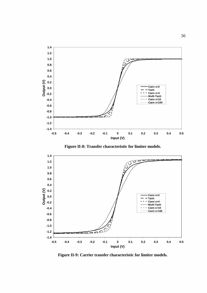
56
-1.4
-1.2
-1.0
-0.8
-0.6
-0.4
-0.2
0.0
0.2
0.4
0.6
0.8
1.0
1.2
1.4
-0.5 -0.4 -0.3 -0.2 -0.1 0 0.1 0.2 0.3 0.4 0.5
Input (V)
Ou
tput
(V
)
Cann s=2TanhCann s=4Multi-TanhCann s=10Cann s=100
Figure II-8: Transfer characteristic for limiter models.
-1.4
-1.2
-1.0
-0.8
-0.6
-0.4
-0.2
0.0
0.2
0.4
0.6
0.8
1.0
1.2
1.4
-0.5 -0.4 -0.3 -0.2 -0.1 0 0.1 0.2 0.3 0.4 0.5
Input (V)
Ou
tput
(V
)
Cann s=2TanhCann s=4Multi-TanhCann s=10Cann s=100
Figure II-9: Carrier transfer characteristic for limiter models.

57
Common emitter configuration of a bipolar or heterojunction bipolar (HBT)
transistor has an exponential collector current dependency on the input voltage across
the base emitter junction
( )
( )BE
F T
V t
n vc sI t I e= (II.43)
where
( ) ( ) ,BE BE beV t V V t= +
BEV is the DC value of the base emitter voltage, ( )beV t is the time varying component
of the input signal, /Tv kT q= is the thermal voltage, sI is the collector saturation
current, and Fn is the nonideality factor [76]. There is an additional collector voltage
nonlinearity due to the Early voltage effect that is not considered here. In addition, the
base current is also exponentially dependent on the base emitter voltage
( )
( )BE
F T
V t
n vsB
F
II t e
β= (II.44)
where Fβ is the forward collector to base current gain. The base current nonlinearity
is of interest in cases where significant distortion of base voltage leads to
crossmodulation between the input signal and the base distortion components [77, 78].
The Taylor series expansion for the collector current is
0
( )1( ) .
!
k
BEc s
k T
V tI t I
k v
∞
=
= ∑ (II.45)
Separating out the DC bias component from the input signal leads to a simple
behavioral model for a bipolar or heterojunction common emitter amplifier

58
0
( )1( ) .
!
BE
F T
kV
n v bec s
k T
V tI t I e
k v
∞
=
= ∑ (II.46)
However, common emitter amplifiers exhibit gain compression at high output signal
whereas (II.46) is an exponential function that grows without bound. Gain
compression for a common emitter amplifier arises from either a limitation in the base
current drive supplied by the previous stage, voltage swing at the collector, or by local
feedback.
The common emitter differential pair amplifier shown in is a circuit widely used in
RFIC and analog IC designs. The large signal transfer function of the bipolar polar
differential pair is a hyperbolic tangent function of the input signal
( )
( ) tanh2
beo E
T
V tv t RI
v
−= (II.47)
with limiting value of ERI and a gain of ( ) /(2 )E TRI v . The linearity of the circuit can
be improved at the expense of lower gain by adding either shunt feedback resistance
from the output to input or by adding series feedback resistor in the emitters; however,
the noise performance suffers significantly since the gain is reduced but the noise
contribution of devices is not.

59
inv
ov
R R
Q1 Q2
EI
Vcc
Figure II-10: Bipolar differential pair amplifier.
The linearity of the differential pair can be improved by implementing parallel
devices with particular area ratios or fixed areas with differing current ratios to
introduce offset hyperbolic tangent transfer characteristics [79]. The technique is
known as multi-tanh due to the summation of multiple offset hyperbolic tangent
functions. The large signal transfer characteristic for a general case of N offset
differential pairs is [80]
1
( )( ) tanh .
2j
Nbe j
o Ej T
V t Vv t R I
v=
− + = ∑ (II.48)
where jV is an offset voltage. One practical form of the multi-tanh circuit is the so
called triplet, named for the number of differential pairs, is shown in Figure II-11
consisting of one differential pair in parallel with two differential pairs with scaled
emitter areas to generate ± offset voltages in the hyperbolic tangent transfer functions
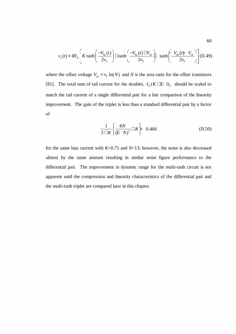
60
( ) ( ) ( )
( ) tanh tanh tanh2 2 2
be be os be oso E
T T T
V t V t V V t Vv t RI K
v v v
− − + − −= + + (II.49)
where the offset voltage ln( )os TV v N= and N is the area ratio for the offset transistors
[81]. The total sum of tail current for the doublet, ( 1 1)EI K + + , should be scaled to
match the tail current of a single differential pair for a fair comparison of the linearity
improvement. The gain of the triplet is less than a standard differential pair by a factor
of
2
1 80.466
2 (1 )
NK
K N
+ = + + (II.50)
for the same bias current with K=0.75 and N=13; however, the noise is also decreased
almost by the same amount resulting in similar noise figure performance to the
differential pair. The improvement in dynamic range for the multi-tanh circuit is not
apparent until the compression and linearity characteristics of the differential pair and
the multi-tanh triplet are compared later in this chapter.

61
ov
R R
Q1 Q2
EKIEIEI
N N
Q3Q5 Q4 Q6
inv inv
Vcc
Figure II-11: Multi-tanh triplet differential amplifier.
The carrier gain compression characteristic of the hyperbolic tangent, Cann limiter,
and the multi-tanh models are shown in Figure II-12. The input power independent
variable is defined as the power when the shunt input impedance is 50Ω . The linear
gain for each model was set to 1/(2 )Tv which is the same as the differential pair
amplifier with a ERI product of unity. The gain of the multi-tanh triplet model from
(II.49) is 6.6 dB lower than a differential pair for the same bias current; however, the
limiting output value is the same. The input referred one dB gain compression point
for each of the models is shown in Table II-1. The input compression point for the
Cann model is higher for models with sharper transition factors because the signal does
not compress until it approaches the knee value whereas the softer transition models
start to compress well before the knee value. The multi-tanh triplet response benefits
from both an increase in the sharpness and reduction in gain in comparison to the

62
hyperbolic tangent function resulting in a 11 dB improvement in the input compression
point relative to hyperbolic tangent function and a net improvement in output dynamic
range of 4.4 dB.
10
12
14
16
18
20
22
24
26
28
-35 -30 -25 -20 -15 -10 -5 0 5 10Input Power (dBm)
Gai
n (
dB
)
Cann s=2TanhCann s=4Cann s=10Cann s=100Multi-Tanh
Figure II-12: Carrier gain compression characteristics for nonlinear models.
Table II-1: Comparison of sinusoidal P1dB input gain compression.
Nonlinear
Model
Sinusoidal Input
P1dB (dBm)
Multi-tanh Triplet -8
Tanh -19
S=2 -20
S=4 -16
S=10 -14
S=100 -14

63
II.6 Power Series Model
The complex power series coefficients for modeling AM-AM and AM-PM
characteristics are obtained by using either a Taylor series expansion of a known
nonlinear function or a least squared error fit of the series coefficients to a measured,
simulated, or derived complex gain characteristic for the device under test. The AM-
AM and AM-PM characteristics are expressed in rectangular form as
[ ] [ ] [ ] [ ] ( ) ( )
Re Im
Re ( ) e Im ( ) e
o o o
j A t j A tin in
v v j v
F A t v j F A t v− Φ − Φ
= +
= +
ɶ ɶ ɶ ɶ ɶ (II.51)
where invɶ and ovɶ are the complex envelopes of input and output signals respectively.
The rectangular form is also known as a quadrature model of the bandpass nonlinearity
[7, 51]. A graphical representation of a quadrature model is shown in Figure II-13.
[ ] [ ] )()(Re tAjetAF Φ−
[ ] [ ] )()(Im tAetAF Φ j
∑inv~ ov~
Figure II-13: Quadrature AM-AM AM-PM model.
The real and imaginary components are separated and each fitted to a real power series
expansion using a least mean squared error fit to the data

64
3 5Re1 Re3 Re5 Re
3 5Im1 Im3 Im5 Im
Re
Im .
mo in in in m in
mo in in in m in
v a v a v a v a v
v a v a v a v a v
= + + + +
= + + + +
ɶ ɶ ɶ ɶ ɶ…ɶ ɶ ɶ ɶ ɶ… (II.52)
An odd power series is used because only odd terms contribute to the fundamental
input/output gain characteristic as described in section II.1.
The power series model is general representation of a memoryless nonlinear
characteristic; however, there are other methods by which a power series can be
obtained. A Taylor series expansion of the nonlinear characteristic is a possibility for
analytic models or for measurement data with smooth numerical derivatives. The thn order Taylor series expansion of a function, ( )f x , about a point a, is defined as
2 ( )( )( ) ( )( )
( ) ( ) ( )( ) .2! !
n nf a x a f a x af x f a f a x a
n
′′ − −′= + − + + +⋯ (II.53)
For example, the Taylor series expansion for the hyperbolic tangent model is
( )
( )
2 12 22
1
2 2 1tanh ( ) ( ) ; ( )
2 ! 2
kk kk
in in ink
Bg gL v t L v t v t
L k L
π−
∞
=
− = < ∑ (II.54)
where 2kB are Bernoulli numbers [82]. Notice that the hyperbolic tangent expansion
generates only odd order power series coefficients. The Cann model from (II.42) was
shown to be more flexible by providing independent model parameters for gain, limiting
value, and sharpness of the limiting transition; however, analytically the Cann model
has problems with particular derivatives depending on the value s, the sharpness
parameter [68]. In particular, the third-order derivative does not exist when s is an
even integer and, for 2s > , the third-order term of the Taylor series is zero. Thus for
a two-tone input signal the decibel slope of the third-order intermodulation distortion
term will not be 3:1 in the small signal region of operation whereas many physical
limiting amplifiers exhibit a clear 3:1 ratio at low signal levels. However, there are

65
notable exceptions to the 3:1 ratio such as the multi-tanh circuit [80] which exhibits
nulls in the third harmonic distortion term.
Another issue with the Taylor series expansion is the minimum order required to
accurately represent an amplifier operating in the gain compression region. The range
of validity of a model is defined as the peak signal level for which the model agrees
with the measured or analytical data. The valid power range is defined by the peak to
average of the input signal level where the maximum input power is the maximum peak
signal minus the peak to average of the signal. The model needs to be valid well into
the gain compression region, at least several decibels of compression, to accurately
model high level distortion products. A plot of the Taylor series expansions from
(II.54), of the hyperbolic tangent function (II.47), for odd orders 23, 49, and 99 are
shown in Figure II-14. Notice that none of the Taylor series expansions adequately
represent the hyperbolic tangent function in the fully limited region of the nonlinear
characteristic. Moreover, there is only an incremental improvement in the range for a
doubling of the order of the expansion. This implies that a Taylor series expansion of
very high order is necessary to represent the hyperbolic tangent function in the limiting
region of operation. Recall that the number of spectral terms required for calculation
of the output power spectrum (II.25) is the square of the number of series coefficients
in the model 2[( 1) / 2]N − . Thus it is not efficient to use high order series expansions
when using the autocorrelation method for analyzing spectral regrowth.
A least squares fit of a power series to the nonlinear gain characteristic for the
carrier signal is an alternative method for obtaining a power series behavioral model.
The approximate least mean squared error solution is formulated from an over
determined system of equations by applying (II.52) with a sequence of input output
sample pairs greater than the number of coefficients included in the expansion

66
1 1 1 1 1
2 2 2 2 2
3 5Re1 Re3 Re5 Re
3 5Re1 Re3 Re5 Re
3 5Re1 Re3 Re5 Re
Re
Re
Rei i i i i
mo in in in m in
mo in in in m in
mo in in in m in
v a v a v a v a v
v a v a v a v a v
v a v a v a v a v
= + + + +
= + + + +
= + + + +
ɶ ɶ ɶ ɶ ɶ…ɶ ɶ ɶ ɶ ɶ…⋮ ⋮ ⋮ ⋮ ⋮ ⋮ɶ ɶ ɶ ɶ ɶ… (II.55)
where i denotes the ith input/output sample pair. Separating the approximation
equations into matrix form
11 1 1
2 2 22
3
13
3
3
Re
Re
ˆRe i i ii
mo in in in
min in ino
mmin in in
o
v v v v a
v v vv a
av v vv
= ɶ ɶ ɶ ɶ⋯ɶ ɶ ɶɶ ⋯ ⋮⋮ ⋮ ⋮⋮ ɶ ɶ ɶ⋯ (II.56)
or in vector notation
.o inv = V a (II.57)
We want to find a solution where the error vector between the approximated and actual
output values is orthogonal to the actual data
inV e = 0 (II.58)
where
.o ine = v - V a
Solving (II.58) for a yields the least mean squared error approximation of the output
voltage by the power series model provided the columns of the input voltage matrix are
independent
( )-1T Tin in in oa = V V V v (II.59)

67
where ( )-1T Tin in inV V V is also know as the pseudo inverse of the overdetermined system
of equations [83].
A plot of the least squares fit of the hyperbolic tangent function for odd order 23 is
shown in Figure II-14. The least squares model fits well into the limiting region of the
nonlinear gain characteristic with just twelve terms of the expansion. A least squares fit
to odd order 39, twenty coefficients, is enough to represent the full transfer
characteristic of the hyperbolic tangent function; however, functions with sharper
transitions to limiting require higher order fits to represent the function far into limiting.
A least squares fit of odd order twelve was applied to each of the nonlinear carrier
transfer functions shown in Figure II-12. An order of twelve was selected as a tradeoff
between goodness of fit to the nonlinear characteristic in the limiting region and the
resulting number of spectral terms needed to calculate the output power spectrum from
(II.25). A plot of the carrier gain characteristics from each of the least squares power
series models is shown in Figure II-15. The full output range is shown to highlight the
valid range of operation for each of the models. In general, the valid range of
operation is less for models with sharper nonlinear transition into compression because
additional series coefficients are needed to accurately fit the sharper transition over a
wider range of signal levels.

68
-1.2
-1.0
-0.8
-0.6
-0.4
-0.2
0.0
0.2
0.4
0.6
0.8
1.0
1.2
-0.25 -0.20 -0.15 -0.10 -0.05 0.00 0.05 0.10 0.15 0.20 0.25
Input Voltage (V)
Ou
tpu
t V
olta
ge
(V)
TANHLS 23Taylor 23Taylor 49Taylor 99
Figure II-14: Least squares and Taylor series expansion of Ltanh(ving/L).
12
14
16
18
20
22
24
26
28
-30 -25 -20 -15 -10 -5 0
Input Power (dBm)
Gai
n (
dB
)
Cann s=2
TanhCann s=4
Multi-Tanh
Cann s=10Cann s=100
Figure II-15: Carrier gain characteristic of power series limiter models.

69
II.7 Spectral Results
Spectral analysis of the limiter models requires evaluation of (II.25) using the least
squares fitted power series model for each limiter and the 2[( 1) / 2]N − precomputed
spectral terms. The spectral terms are computed by evaluating the 2[( 1) / 2]N −
autocorrelation estimates using (II.24) and (II.21) then taking the FFT of each
correlation term and finally saving all the spectral terms in a single file. A spectral file
only needs to be generated once for each signal of interest. The power of the input
signal used to generate the spectral file is normalized to a convenient value, in this case
0 dBm or 1 mW, such that the power of each spectral term is simply scaled by the ratio
of the desired input power to the normalized input power raised to the appropriate
power of the spectral term
( )( )
( )
( )( )2 1 2 1
2 1
2 1 2 1 n m
n m
innormn m
norm
pS S
p + +
+ +
+ +
= ɶ ɶ (II.60)
where the subscript norm denotes the normalized input power of the spectral term.
The output spectrum is calculated by summing the product of the scaled spectral terms
from (II.60) by the corresponding power series coefficient *2 1 2 1n ma a+ +ɶ ɶ . A flow chart of
the spectral calculation is shown in Figure II-16. A sweep of the input power is easily
performed by sweeping the pin variable over the power range of interest and
recalculating the sum of spectral terms.

70
Construct InputSignal
ComputeAutocorrelation
Terms
FFT to GenerateSpectral Terms
Scale and SumSpectral Terms
MeasureACPR
Input AM-AM andAM-PM Data
Least Squares Fitto Complex
Power Series
Set Input Power
Input Files
Save Coefficientsto Text File
Save SpectralTerms to a Binary
File
Figure II-16: Flow chart for power spectrum calculation.

71
An example plot of the composite, gain compression/expansion, and distortion
power spectrums for the hyperbolic tangent limiter model are shown in Figure II-17.
The power spectrum for the gain compression/expansion terms from (II.26) is nearly
identical to the spectrum of the input signal. The out-of-band spectrum is limited by
the finite rejection of the CDMA baseband FIR filter. Notice that the out of band
distortion of the composite output power spectrum is also limited by the finite rejection
of the baseband filter response. However, the separated distortion spectrum clearly
shows the distortion components below the limiting value of the input signal.
A composite plot of the output power spectrum for each of the limiter models with
a CDMA IS-95 reverse link input signal applied and an output power of 6 dBm is
shown in Figure II-18. For the same output power, the out of band distortion is
highest for the softer limiter models like the Cann s=2 and hyperbolic tangent models,
and lowest for models with a sharper nonlinear transition. Close in distortion spectrum
for the triplet multi-tanh model is roughly 10.5 dB lower than the hyperbolic tangent at
6 dBm output power. The spectrum of the input signal limits the measurable output
power spectrum at far offsets to the carrier which is why the far out spectrums
converge to nearly the same value at offsets greater than 4 MHz.
Fortunately, autocorrelation analysis permits separation of the distortion
components from the gain compression/expansion components of the output spectrum
as was mentioned earlier in this chapter. The distortion power spectrum from (II.27) is
shown in Figure II-19 for each of the limiter models. Now the out of band distortion is
limited by the nonlinear transformation of the input signal resulting in a significantly
lower power spectrum than the input signal itself. Of greater interest is the inband
distortion which is hidden by the desired signal when viewing the composite power
spectrum. Again the inband distortion is higher for models with softer limiting
characteristic and correspondingly lower for models with a sharper transition region.

72
However, there is a greater difference between the inband distortion compared to the
out of band distortion between the hyperbolic tangent and triplet multi-tanh models.
This may indicate that the signal waveform quality factor, ρ, will degrade more rapidly
than the increase in the out of band distortion.
-120
-110
-100
-90
-80
-70
-60
-50
-40
-30
-20
-5 -4 -3 -2 -1 0 1 2 3 4 5
Frequency (MHz)
Po
wer
Sp
ectr
um
(d
Bm
/2.4
kH
z)
Composite SpectrumGain Comp./Exp. SpectrumDistortion Spectrum
Figure II-17: Spectrum components from autocorrelation analysis.

73
-110
-100
-90
-80
-70
-60
-50
-40
-30
-20
-10
-5 -4 -3 -2 -1 0 1 2 3 4 5
Frequency (MHz)
Po
wer
Sp
ectr
um
(d
Bm
/2.4
kH
z)
Cann s=2TanhCann s=4MTanhCann s=10Cann s=100
Figure II-18: Total output power spectrum at 6 dBm for each limiter model.
-120
-110
-100
-90
-80
-70
-60
-50
-40
-30
-20
-5 -4 -3 -2 -1 0 1 2 3 4 5
Frequency (MHz)
Po
wer
Sp
ectr
um
(d
Bm
/2.4
kH
z)
Cann s=2TanhCann s=4MTanhCann s=10Cann s=100
Figure II-19: Distortion spectrum at 6dBm output power for each limiter model.

74
Power sweep characterization of ACPR is important to understanding the nonlinear
behavior of a transmitter circuit. Typically much of the design effort is spent
optimizing ACPR performance at the maximum output power specification in an effort
to maximize efficiency while meeting the ACPR specification limits; however, it is
possible for the ACPR performance to degrade with decreasing drive level and the
ACPR specifications apply at reduced output power levels. An input power sweep was
performed from -50 dBm to -5 dBm in 0.5 dB steps to obtain the ACPR versus output
power characteristic for each of the models. The separated distortion spectrum was
used to measure ACPR to eliminate limiting the measurement by the baseband filter
response of the input signal. The ACPR versus output power plots for each of the
limiter models is shown in Figure II-20 and Figure II-21 for distortion offsets of 885
kHz and 1.98 MHz respectively. These two offsets correspond to those specified for
the adjacent and alternate channel ACPR measurement in the IS-95 CDMA
specification [2]. For these plots, the distortion spectrum was compared against the
main channel power to eliminate the effects of the baseband filter response limiting the
minimum distortion measurement.
There are striking differences between ACPR produced by the different models.
The hyperbolic tangent and Cann s=2 models both exhibit an ACPR to output power
ratio of 2:1 which is expected if the slope of the spectral regrowth versus input power
is 3:1 and the desired signal versus input power is 1:1. A plot of the ACPR slope
versus output power is shown in Figure II-22. A slope of 2:1 is expected for most
class A or class AB amplifiers at lower output power levels where the third order term
of the nonlinearity should dominate the distortion term. The triplet multi-tanh, Cann
s=10, and Cann s=100 models exhibit a 2:1 slope at low output power level; however,
there are noticeable notches in the ACPR response in the 0 dBm to 6 dBm output
power range. The Cann s=4 model has a notch at lower output power levels, around -

75
18 dBm, and the slope appears to be asymptotically approaching 2:1 at lower output
power levels. The multi-tanh exhibits one notch while the Cann s=10 and s=100
models exhibit two notches back to back which is also evident in the slope plots where
there are one and two inversions in the slope. It is interesting that the slope of the
Cann model approaches 2:1 despite the odd behavior reported about the derivates [68].
There are also differences in the ACPR performance of the second offset at 1.98
MHz. The second offset is generally thought to be dominated by fifth order or higher
nonlinearities because the offset falls outside of the spectrum where the third order
distortion term dominates. This is equivalent to a two tone intermodulation distortion
test where the input tone spacing is ± 495 kHz and the third order intermodulation
terms would appear at ± 990 kHz and the fifth order terms at ± 1.98 MHz. This is true
for the hyperbolic tangent and Cann s=2 models at higher output power levels where
the ACPR slope visually appears to be 4:1; however, at lower output power levels the
slope decreases to 2:1 indicating a third order dominant term. The other models reveal
a more complicated response at the second offset; however, all but the Cann s=4
models indicate a third order dominance at low output power levels. It should also be
noted that the second offset distortion contributions are low enough, at lower output
power levels, to have little significance to system performance.
Differences in ACPR between the triplet multi-tanh versus the hyperbolic tangent
models are of interest since each represents at physical circuit response. At lower
output power levels the triplet multi-tanh model has an approximate 13 dB
improvement in the ACPR than the hyperbolic tangent model at the same output power
level. Near the notch of the triplet multi-tanh response the ACPR improvement is as
much as 35 dB. After the notch the distortion rises and approaches that of the
hyperbolic tangent function at high output power levels. This result shows that the
multi-tanh technique of linearity improvement provides substantial improvement in

76
linearity performance for the same output power and bias current of a differential pair
circuit.
Also of interest is the gain compression characteristic when a modulated signal is
driving the nonlinear model [84]. The CDMA waveform has a significantly different
amplitude distribution compared to a sinusoidal waveform, so it is anticipated that the
gain compression characteristics should show some differences. The CDMA gain
compression characteristic is measured by comparing the difference in input power and
output power for the desired CDMA signal channel. A plot of CDMA gain
compression is shown in Figure II-23. Similar to the sinusoidal carrier compression
results from Figure II-12, the CDMA gain compression is more significant for models
with a softer nonlinear transition compared to models with a sharper transition. A
comparison the CDMA input referred one dB compression point to the sinusoidal
compression results for the nonlinear models is shown in Table II-2. As expected the
wider amplitude variations of the CDMA signal contribute more to the gain
compression resulting in a slightly lower input referred compression point compared to
a sinusoidal input signal.

77
Table II-2: Comparison of CDMA P1dB input gain compression.
Nonlinear Model CDMA Input
P1dB (dBm)
Delta to
Sinusoid (dB)
Multi-tanh Triplet -9.0 -1.0
Tanh -19.5 -0.5
S=2 -21.0 -1.0
S=4 -16.5 -0.5
S=10 -15.0 -1.0
S=100 -14.5 -0.5

78
-160
-140
-120
-100
-80
-60
-40
-20
0
-22 -20 -18 -16 -14 -12 -10 -8 -6 -4 -2 0 2 4 6 8 10 12
Output Power (dBm)
Ad
jace
nt
Ch
ann
el P
ow
er (
dB
c)
Cann s=2TanhCann s=4Multi-TanhCann s=10Cann s=100
Figure II-20: Adjacent channel power at 885 kHz offset for limiter models.
-160
-140
-120
-100
-80
-60
-40
-20
0
-22 -20 -18 -16 -14 -12 -10 -8 -6 -4 -2 0 2 4 6 8 10 12
Output Power (dBm)
Ad
jace
nt
Ch
ann
el P
ow
er (
dB
c)
Cann s=2TanhCann s=4Multi-TanhCann s=10Cann s=100
Figure II-21: Adjacent channel power at 1.98 MHz offset for limiter models.

79
-4
-2
0
2
4
6
8
10
12
-24 -22 -20 -18 -16 -14 -12 -10 -8 -6 -4 -2 0 2 4 6 8 10 12
Output Power (dBm)
AC
PR
to
Ou
tpu
t P
ow
er S
lop
e (d
Bc/
dB
m)
Cann s=2TanhCann s=4Multi-TanhCann s=10Cann s=100
Figure II-22: Slope of ACPR versus output power.
15
16
17
18
19
20
21
22
23
24
25
26
27
28
29
30
-40 -38 -36 -34 -32 -30 -28 -26 -24 -22 -20 -18 -16 -14 -12 -10 -8 -6 -4
Input Power (dBm)
CD
MA
Gai
n (
dB
)
Cann s=2
TanhCann s=4
Multi-Tanh
Cann s=10
Cann s=100
Figure II-23: CDMA Gain compression characteristic.

80
II.8 Summary
This chapter presented an approach to modeling the AM-AM and AM-PM carrier
characteristics of nonlinear circuit using a complex power series behavioral model using
the measured or simulated AM-AM and AM-PM response of the circuit. Power series
coefficients are obtained from a least squared error fit of the coefficients to the
rectangular representation of the AM-AM and AM-PM response of the circuit. Least
squared error formulation was shown to greatly enhance the dynamic range of the
behavioral model compared to a Taylor series expansion of the same or even higher
order. The properties of several limiting amplifier models were introduced with
progressive differences in sharpness of the transition from linear to limiting operation.
Power series models were fit to each of the models to use in later analysis.
The fundamental complex envelope response of a modulated carrier applied to a
complex power series model was presented. Distortion components that are centered
about the carrier frequency are separated from other components using a binomial
expansion of each exponential of the complex envelope. The time average
autocorrelation is taken at the output of the model resulting in a general output
autocorrelation function representing the nonlinear transformation of modulated carrier
applied to a bandpass nonlinearity. The output power spectrum is obtained from the
Fourier transform of the output autocorrelation function. The output spectrum is
separated into gain compression/expansion components, which are those components
associated with the carrier signal, and distortion components. Autocorrelation analysis
is applied to power series representations of each limiter model and the spectral and
ACPR results are presented. The analysis shows how characteristics of each model
influence the power spectrum results. Models with softer limiter characteristics
generally have worse distortion performance than those with sharper nonlinear

81
transition from linear to limiting operation. Even at reduced output power levels the
sharper transition nonlinearities have significantly better linearity.
The text of this chapter, in part, is a reprint of the material as it appears in our
published papers in IEEE Conferences [CICC01 and IMS01] and publication in IEEE
Transactions on Microwave Theory and Techniques [submitted 2003]. The dissertation
author was the primary investigator and author of these papers.

82
III. Statistical Analysis of Bandpass Nonlinearities
Modern wireless communication systems utilize increasingly more complex
modulation schemes to increase capacity of the system and raise the available
bandwidth for data users. The first CDMA systems only utilized a single signal or
orthogonal Walsh code channel from the handset to the base station. However newer
CDMA2000 1x, EvDo, and DV standards support synchronous reverse links with a full
time pilot signal and a multitude of control, paging, and traffic Walsh code channels.
The forward link always supported multiple code channels for each of the users and a
pilot code channel [85]. In general, the more code channels that are added the wider
the amplitude variation of the signal. This is a result of a statistical law of random
signals known as the central limit theorem which states that the sum of independent
random variables tends towards a Gaussian distribution with increasing number of
variables [61]. The statistical properties of most practical communication signals are
not known in an analytical form; however, statistical modeling of signals is possible
through the central limit theorem when several independent signals are summed
together. This opens the door to the use of statistical mathematics to calculate the
power spectrum of wireless signals transformed by nonlinear wireless circuits.
The previous section presented the general case of a carrier signal with arbitrary
amplitude and phase modulation passed through a nonlinear behavioral model. The
generality of the analysis lead to a solution with ( )[ ]22/1−N spectral terms for a
nonlinearity represented by anthN order odd power series. Information theory studies
methods for evaluating signals and transformations of signals by exploiting the
statistical properties of the signal provided the statistical properties are known and are
applicable to the problem at hand. Statistical signal analysis often leads to evaluation of
complicated mathematical expressions; however, the potential benefits of the analysis

83
include closed form and reduced order solutions over the general autocorrelation
formulation presented in the previous chapter. The benefit for nonlinear circuit analysis
is reduced order equations which yield clearer insight into how the signal and circuits
interact to generate the observed output spectrum.
This section presents a method for predicting spectral regrowth based on the
nonlinear transformation of the statistics of the input signal. A scheme that is simple to
calculate, and therefore more readily available to the practicing engineer seeking to
estimate the nonlinear transfer response, is developed. The proposed formulation seeks
to provide design insight into how the nonlinearity affects the output spectrum, by
developing a modular approach that considers the successive transformation of the
input statistics through the modulation scheme and the nonlinearity itself. The output
power spectrum is estimated from an analytical expression for the output
autocorrelation function that describes the transformation of a complex Gaussian signal
when passed through a bandpass nonlinearity. The nonlinearity is modeled by a
complex power series obtained from the measured or simulated AM-AM and AM-PM
characteristics of the device.
III.1 Statistical Moments
In the previous section, the analysis is based upon evaluation of a general time
averaged autocorrelation function, or sum of time averaged moments, of the output
signal. The bridging principle between the time and statistical domains is equivalence
of statistical and time averaged moments for signals that are ergodic in regards to the
autocorrelation function. Ergodicity refers to a property where the ensemble averages
of random process converge to the time average of one realization of the process, in
the limit, as t goes to infinity [86, 87]

84
*
*
( ) ( ) ( )
1lim ( ) ( )
2
( ) .
zz
T
TT
zz
R E z t z t
z t z t dtT
τ τ
τ
τ
→∞−
= + = +
= ℜ
∫ɶ ɶ ɶ ɶ ɶɶ (III.1)
This is a very useful, and remarkable, property that permits substitution of time
averages for statistical averages. Moments for certain random processes can be
formulated from known properties of the process, but evaluation of the moments from
the statistical description may be mathematically difficult. In those cases, the moments
may be evaluated by substituting time average autocorrelation functions for the
statistical moments. There is a net reduction in complexity when the moment
formulation leads to fewer autocorrelation terms than the general time average
autocorrelation function formulation.
In addition to egodicity, a random process must be a stationary process to permit
(III.1) to be valid. Strict sense stationarity is a property of a random process where all
the moments of the process are dependent only on the time difference between samples
of the process or put another way the process is invariant with the absolute time each is
variable is sampled. Only the first and second moments are required to be invariant
with absolute time for (III.1) to be valid, such a process is called wide sense stationary
(WSS). Without WSS and ergodicity properties the second moment of a random
process is defined as
[ ]
*1 2 1 2
*1 2 1 2 1 2
( , ) ( ) ( )
( ) ( ) ( ), ( )
zz
ZZ
R t t E z t z t
z t z t f z t z t dt dt∞ ∞
−∞ −∞
= = ∫ ∫ɶ ɶ ɶɶ ɶ ɶ ɶ (III.2)
which requires knowledge of the joint probability density function, 1 2[ ( ), ( )]ZZf z t z tɶ ɶ of
the random process. Generally, the joint probability density function is not known.

85
Fortunately, most communication signal problems fit the WSS and ergodic criterion
such that the statistical moments can be replaced by the time average autocorrelation
function.
III.2 Gaussian Random Process
The statistical properties of the Gaussian or normal random variable is one of the
most well known and studied signals in information theory. The popularity of the
Gaussian random process is attributed to its relatively straightforward mathematical
properties and because of the central limit theorem, which states that the sum of
identically distributed, zero mean, independent random processes tends to a zero mean
Gaussian distribution. This is a remarkable and useful property since there are many
practical problems, such as semiconductor noise, which involve sums of random
processes which are not Gaussian. A Gaussian or normal random process follows the
Gaussian probability density function [59]
2
22
( )1( ) exp
22X
XXX
xf x
µσπσ
−= − (III.3)
where Xµ is the mean value of the process and 2Xσ is the variance. Typically wireless
communication system problems deal with zero mean processes because no information
is contained in the mean and nonzero mean processes cause practical problems of
numerical headroom for digital signal processing (DSP) and voltage/current headroom
issues for baseband and RF circuits.
III.3 Transformation of a Complex Random Process
The digital quadrature-modulated signal, )(~ tz , is statistically modeled as the
complex addition of two independently filtered stationary random processes, x(t) and
y(t), each assumed to be zero mean:

86
)()()(~ tjytxtz += (III.4)
where the tilde is used to indicate a quadrature signal. The variables here are voltage-
like quantities; the power of each is proportional to the corresponding autocorrelation
function, and each is assumed to be stationary and identically distributed. Thus the
notation is simplified by introducing subscripts to indicate quantities at different times:
222111
21
21
~,~)(,)(
)(,)(
jyxzjyxz
tyytyy
txxtxx
+=+=+==+==
ττ
(III.5)
Simplification of the notation is possible since the stationary assumption permits the
time variable to be removed from the notation because the autocorrelation and
crosscorrelation sequences only depend on the time difference, τ, and not on absolute
time. The autocorrelation function of a complex stationary random process )(~ tz is
defined as
]~~[)](~)(~[)(~ *
21* zzEtztzERzz =+= ττ (III.6)
where E[ ] is the expected value operator and * denotes the complex conjugate. Since
random processes x(t) and y(t) are stationary, the following autocorrelation and
crosscorrelation identities apply :
0][][)0(
][][)()(
][][][][)0(
][][)()(
2211
1221
22112211
2121
===
−==−=====
===
yxEyxER
yxEyxERR
yyEyyExxExxER
yyExxERR
xy
yxxy
xx
yyxx
ττ
ττ
(III.7)
The autocorrelation of the quadrature baseband process )(~ tz , can now be written as

87
)(2)(2
)]([
)])([(
]~~[)](~)(~[)(~
21122121
2211
*21
*
ττ
ττ
xyxx
zz
RjR
yxyxjyyxxE
jyxjyxE
zzEtztzER
−=−++=
−+==+=
(III.8)
)(~ τzzR defines the statistics of the modulator’s output, which is the signal input to the
nonlinear device. It should be noted that the real part of the autocorrelation function is
an even function and the imaginary part is an odd function about 0τ = . The average
power, Pzz, of the input signal, )(~ tz , is proportional to the autocorrelation function
evaluated at τ=0:
)0(2
)0()0(2
)0(~
xx
xyxx
zzzz
AR =
jR-RA
RA P
==
(III.9)
Here A is a power scaling variable used to set the input power level.
The nonlinear device is characterized, in part, using single-tone measurements, and
can be represented as a bandpass nonlinearity with complex transfer characteristic [32]:
[ ]
1
3 51 3 5
( ) ( )
( ) ( ) ( ) ... ( )
Ni
ii
NN
G z t a z t
a z t a z t a z t a z t
==
= + + + +
∑ɶ ɶɶ ɶɶ ɶ ɶ ɶɶ ɶ ɶ ɶ (III.10)
where ia~ are complex power series coefficient and [ ]( )G z tɶ ɶ is the complex power
series representation of an AM-AM and AM-PM characteristic. Only the odd terms
can be determined from single-tone complex compression characteristics, but
fortunately the odd order terms are the most important as they produce intermodulation
distortion in band and adjacent to the desired signal. It is important to realize that
(III.10) represents a general nonlinear transfer characteristic and is not a gain
expression.

88
The autocorrelation function of the signal at the output of the nonlinear device is
found by applying (III.6) to the baseband equivalent polynomial model, (III.10), with
coefficients ia~ :
[ ] [ ]
[ ] [ ] [ ][ ] [ ] [ ][ ] [ ] [ ] ...)~(~~)~(~~~~~~~
)~(~~~)~(~~~~~~
)~(~~~)~(~~~~~~
)~(~)~(~~~~~~~~~
)~(~
)~(~
)(~
*52
51
2
5*3
25
15*3
*2
515
*1
*52
31
*53
*32
31
2
3*2
313
*1
*521
*51
*321
*31
*21
2
1
5*2
*5
3*2
*3
*2
*1
515
31311
2*
1
+++
+++
+++=
++++=
=
zzEazzEaazzEaa
zzEaazzEazzEaa
zzEaazzEaazzEa
zazazazazazaE
zGzGERgg τ
(III.11)
Expanding )(~ τggR results in many algebraically intensive moment manipulations
involving x(t) and y(t). Fortunately, a previous result for the moments of complex
Gaussian random variables [88] can be used to calculate each of the terms in this
expression, namely
[ ][ ] [ ] [ ] =
≠= ∑ tszzEzzEzzE
ts
zzzzzzE
ts
ts
,~~...~~~~
,0~...~~~...~~
*)(
*2)2(
*1)1(
**2
*121
ππππ
(III.12)
where π is a permutation of the set of integers 1,2, , , ,s t… … , and
, 1,2, , , ,iz i s t=ɶ … … denotes a set of complex independent Gaussian random
variables. Application of (III.12) yields the following identity:
* * * * * *1 2 3 4 1 3 2 4 2 3 1 4E z z z z E z z E z z E z z E z z = + ɶ ɶ ɶ ɶ ɶ ɶ ɶ ɶ ɶ ɶ ɶ ɶ (III.13)
and most importantly:
[ ] [ ] )(~
!~~!)~~( *21
*21 τn
zz
nn RnzzEnzzE == (III.14)

89
In addition, any terms including an unequal number of conjugate terms in the
expectation is zero, for example the first order term crossed with the third order term is
3 *1 2( ) 0 .E z z = ɶ ɶ (III.15)
Assuming that the input random process is a complex Gaussian variable and application
the moment theorem (III.12) and resulting identities (III.14), (III.15) allows the
expanded form of the output autocorrelation function, (III.11), to be simplified,
yielding the compact expression:
∑=
=
+++=N
oddnn
nzz
nn
Nzz
NNzzzzgg
RAan
RAaNRAaRAaR
1
2
2332
3
2
1
)(~~!
)(~~!...)(
~~!3)(~~)(
~
τ
ττττ
(III.16)
where A is a power scaling variable used to set the input power level. Evaluation of the
output power spectrum requires an estimate of the input autocorrelation function,
)(~ τzzR , of the complex input process )(~ tz . A closed form analytical expression for the
autocorrelation function is difficult to derive [89]; however, good estimates can be
obtained by using long, independent data sequences passed through a quadrature
modulator. Input autocorrelation is then estimated by applying a sliding discrete
correlator to the sum of the two Gaussian input streams x(t) and y(t), after passing
them through a hard limiter (sign function) and an FIR baseband filter as shown in
Figure II-2. This generates an input stream as defined by the CDMA IS-95 standard
[2]. The output autocorrelation function, (III.16), is then defined by powers of the
input autocorrelation function, an input scaling factor, and the magnitudes of the power
series coefficients. It is interesting to note that each of the cross terms in the expansion
of )(~ τzzR are zero as a result of the moment theorem [88]. The output power
90
spectrum, )(~
fSgg , is obtained as the Fourier transform of the output autocorrelation
from (III.16)
∑∑ ∫∫=
=
∞
∞−
−
∞
∞−
−
=
=
=
N
oddnn
nzz
nn
N
n
fjnzz
nn
fjgggg
RFAan
deRAan
deRfS
1
2
1
22
2
)(~~!
)(~~!
)(~
)(~
τ
ττ
ττ
τπ
τπ
(III.17)
where
2( ) ( ) .n n j fzz zzF R R e dπ ττ τ τ
∞ −
−∞= ∫ɶ ɶ
Thus the output power spectrum is the sum of the individual spectra of each term in the
power series, scaled by its corresponding coefficient and input power level. When
computing the output spectrum, the Fourier transform of each spectral component is
calculated first, then scaled by the input power level and the corresponding power
series coefficient, and added into (III.17) yielding )(~
fSgg . This derivation shows that
only the input autocorrelation function, )(~ τzzR , and the complex power series
description are necessary to estimate the output power spectrum of the nonlinear
device.
III.4 Transformation of a Bandpass Random Process
First consider the case where a carrier frequency is modulated by a real random
process, ( )x t ,
1 1
( ) ( ) ( )2 2
c cj t j tw t x t e x t eω ω−= + (III.18)

91
where 2c cfω π= and cf is the carrier frequency. The modulated carrier is applied to
the input of a nonlinear circuit represented by the complex power series model from
(II.10)
[ ]( )1 /2
2 12 12
0
2 1( ) ( ) .
12c
Nnn
nn
naG z t x t
nω
−++
=
+ = + ∑ ɶɶ ɶ (III.19)
The output autocorrelation function is found by taking the expectation of the output
signal
( ) ( )
( )
*1 2
1 1*2 2
2 1 2 12 1 2 11 22 2
0 0
*2 1 2 12 1 2 11 22
0
( )
2 1 2 1
1 12 2
2 1 2 1
1 12
c cgg
N N
n mn mn m
n m
N
n mn mn m
m
R E G z G z
n ma aE x x
n m
n ma aE x x
n m
ω ωτ− −
+ ++ +
= =
−
+ ++ ++
=
= + + = + + + + = + + ∑ ∑ɶ ɶɶ ɶ ɶɶ ɶɶ ɶ1 1
2 2
0
.
N
n
−
=∑∑ (III.20)
The expectation can only be evaluated if the moments of the random variable are
known. For the case of a zero mean real Gaussian process the moments are given by
[60, 90]
[ ][ ] [ ] [ ]
1 2
1 2 3 4 1
0 ,
...
, .s
s sall distinct
pairsof subscripts
s odd
E x x x
E x x E x x E x x s even−
= ∑ … (III.21)
Expansion of the modulated carrier leads to many cross terms which do not evaluate to
zero as was the case with a complex baseband signal. Here are the moments evaluated
for a seventh order power series expansion

92
n=0, m=0 : [ ] )(21 τxxRxxE =
n=0, m=1 : [ ] [ ] )(3231
321 τxxxoRRxxExxE ==
n=1, m=1 : [ ] )(6)(9 3332
31 ττ xxxxxo RRRxxE +=
n=0, m=2 : [ ] [ ] )(15 22
51
521 τxxxoRRxxExxE ==
n=1, m=2 : [ ] [ ] )(60)(45 3332
51
52
31 ττ xxxoxxxo RRRRxxExxE +==
n=2, m=2 : [ ] )(120)(600)(225 532452
51 τττ xxxxxoxxxo RRRRRxxE ++=
n=0, m=3 : [ ] [ ] )(105 32
71
721 τxxxoRRxxExxE ==
n=1, m=3 : [ ] [ ] )(630)(315 3432
71
72
31 ττ xxxoxxxo RRRRxxExxE +==
n=2, m=3 : [ ] [ ] )(2520)(6300)(1575 533552
71
72
51 τττ xxxoxxxoxxxo RRRRRRxxExxE ++==
n=3, m=3 : [ ] )(5040)(52920)(66150)(11025 75234672
71 ττττ xxxxxoxxxoxxxo RRRRRRRxxE +++=
where .)0(~ == τxxxo RR
Collecting terms of equal order and including power series coefficients for clarity
yields:
the linear term (gain expansion/compression term)

93
22 3
1 3 5 73 15 105 ( )xo xo xo xxa a R a R a R R τ+ + + ɶɶ ɶ ɶ ɶ (III.22)
third order distortion term
)(~~105~10~!3 322
753 τxxxoxo RRaRaa ++ (III.23)
fifth order distortion term
)(~~21~!5 52
75 τxxxo RRaa + (III.24)
and seventh order distortion term
.)(~~!7 72
7 τxxRa (III.25)
Inspection of the terms reveals a pattern to the terms yielding the following expression
for the terms of equal power
212 12
2 1 2 1(2 1)! ( )( )
2 ( )! (2 1)!
Nk
k n kn xxgg xon k
n k
a n RR R
n k k
ττ
−+
+ −+−
=
+=− +∑ ɶɶɶ (III.26)
where the power series coefficients have been included to illustrate which terms are
associated with the series coefficients. Adding in the binomial coefficient terms along
with the power series coefficients yields an expression for the nonlinear output
autocorrelation function term
( ) ( )
212 12
2 12 13
2 1 ! 2 1 ! ( )( ) .
2 ( )!( 1)! ! (2 1)!
Nk
nk n k xxgg xon k
n k
a n n RR R
n k n n k
ττ
−+
++ −−
=
+ +=
− + +∑ ɶɶɶ (III.27)

94
The output autocorrelation function expression for a carrier modulated by a real
Gaussian random process passed through a bandpass nonlinearity is the sum of
nonlinear autocorrelation terms
1
22 1
0
( ) ( ) .
N
kgg gg
k
R Rτ τ
−
+
==∑ɶ ɶ (III.28)
Thus similarly to the complex Gaussian case, the output autocorrelation function is a
sum of ( ) 2/1−N terms for an thN odd order power series; however, here each
autocorrelation term is weighted by a sum of DC powers from other nonlinear terms.
The output autocorrelation function is a closed-form expression in terms of
autocorrelation of the input signal and the sum of the input power weighted by the
power series coefficients. Note that there are only N autocorrelation terms as
compared to 2N for the general time domain case. The output power spectrum is the
Fourier transform of the autocorrelation function
1
22 1
0
( ) ( )
N
kgg gg
k
S f S f
−
+
==∑ɶ ɶ (III.29)
where
( ) ( )
212 1
22 12 13
( )2 1 ! 2 1 !( )
2 ( )!( 1)! ! (2 1)!
Nk
zznk n kgg zon k
n k
F Ra n nS f R
n k n n k
τ−
+++ −−
=
+ +=
− + +∑ ɶɶɶ (III.30)
and
2 1 2 1 2( ) ( ) .k k j fzz zzF R R e dπ ττ τ τ
∞+ + −
−∞= ∫ɶ ɶ
Use of the moment theorem yielded a closed form expression for the output spectrum
and greatly reduced the number of terms in the calculation.

95
III.5 Transformation of a Complex Bandpass Random
Process
The problem is more complicated when extended to the case where a carrier is
modulated by a complex random process. For this case, the output autocorrelation
function is formulated by taking the expectation of the output of the nonlinear amplifier
with a modulated carrier applied to the input from (II.10)
( ) ( )
( ) ( )
( ) ( )
*1 2
1 1*2 2 11 * *2 1 2 1
1 1 2 22 20 0
*1 *2 1 2 1
1 12
( )
2 1 2 1
1 12 2
2 1 2 1
1 12
c cgg
N N
n mn mn mn m
n m
nnn mn m
R E G z G z
n ma aE z z z z
n m
n ma aE z z
n m
ω ωτ− −
+++ +
= =
++ ++
= + + = + + + +
= + + ∑ ∑ɶ ɶɶ ɶ ɶɶ ɶɶ ɶ ɶ ɶɶ ɶ ɶ ɶ ( )1 1
2 2 1*2 2
0 0
.
N N
m m
n m
z z
− −
+
= =
∑∑ ɶ ɶ (III.31)
Thus the power series expansion and resulting cross terms in the autocorrelation
function yield the following expression for the expectation term
( ) ( ) ( )*
11 * *2 1 2 1(2 1)(2 1) 1 1 2 22
2 1 2 1( ) .
1 12
n mn mn mn m n m
n ma aR E z z z z
n mτ
+++ ++ + +
+ + = + + ɶ ɶɶ ɶ ɶ ɶ ɶ (III.32)
The resulting output autocorrelation function is
1 1
2 2
(2 1)(2 1)0 0
( ) ( ) .
N N
gg n mn m
R Rτ τ
− −
+ += =
=∑∑ɶ ɶ (III.33)
Evaluation of the expectation function is more complicated for this case due to the
complex conjugate terms generated by the envelope of the carrier. The cross terms do
not evaluate to zero as they did for the complex random process case. Each term of
the expectation is evaluated by applying the complex Gaussian moment theorem (II.10)
. Here are the first ten terms of the expansion

96
n=0, m=0 : [ ] )(~~~ *
21 τzzRzzE =
n=0, m=1 : ( )[ ] zozz RRzzzE )(~
2~~~ 2*221 τ=
n=1, m=1 : ( )[ ] )(~
)(~
2)(~
4~~~~ *222*2
*12
21 τττ zzzzzozz RRRRzzzzE +=
n=0, m=2 : ( )[ ] 23*2
221 )(
~6~~~
zozz RRzzzE τ=
n=1, m=2 : ( )[ ] zozzzzzozz RRRRRzzzzE )(~
)(~
12)(~
12~~~~ *233*2
*1
22
21 τττ +=
n=2,m=2: ( ) ( )[ ] [ ]2*32*243*2
2*1
22
31 )(
~)(
~12)(
~)(
~72)(
~36~~~~ τττττ zzzzzozzzzzozz RRRRRRRzzzzE ++=
n=0, m=3 : ( )[ ] 34*2
321 )(
~24~~~
zozz RRzzzE τ=
n=1, m=3 : ( )[ ] 2*244*2
32
*1
21 )(
~)(
~72)(
~48~~~~
zozzzzzozz RRRRRzzzzE τττ +=
n=2, m=3:
( ) ( )[ ] [ ] zozzzzzozzzzzozz RRRRRRRRzzzzE2*33*254*
2
2*1
32
31 )(
~)(
~144)(
~)(
~432)(
~144~~~~ τττττ ++=
n=3, m=3:
( ) ( )[ ][ ] [ ]3*422*3
4*264*2
3*1
32
41
)(~
)(~
144)(~
)(~
1728
)(~
)(~
2592)(~
576~~~~
ττττ
τττ
zzzzzozzzz
zozzzzzozz
RRRRR
RRRRRzzzzE
+
++=

97
where .)0(~ == τzzzo RR
Collecting terms of equal order and adding in the power series coefficients for clarity
yields the linear gain compression/expansion term
)(~~120~24~6~2~ 24
93
72
531 τzzzozozozo RRaRaRaRaa ++++ (III.34)
third order distortion term
)(~
)(~~240~36~6~!2!1 *223
92
753 ττ zzzzzozozo RRRaRaRaa +++ (III.35)
fifth order distortion term
[ ]2*322975 )(
~)(
~~120~12~!3!2 ττ zzzzzozo RRRaRaa ++ (III.36)
seventh order distortion term
[ ]3*42
97 )(~
)(~~20~!4!3 ττ zzzzzo RRRaa + (III.37)
and the ninth order distortion term
[ ] .)(~
)(~~!5!4
4*52
9 ττ zzzz RRa (III.38)
Inspection of the terms reveals a pattern to the terms yielding the following expression
for the terms of equal power
211 *
22 1 2 1
( ) ( )!( 1)!( )
( )! !( 1)!
N kkzz zzk n kn
gg zon k
R Ra n nR R
n k k k
τ ττ
−+
+ −+
=
+ =− +∑ ɶ ɶɶɶ (III.39)
where the power series coefficients have been included to illustrate which terms are
associated with the series coefficients. Adding in the binomial coefficients yields, after
simplification, the expression for the nonlinear output autocorrelation function term

98
( )( )
211 *
22 12 1
2
( ) ( )2 1 !( )
2 ! !( 1)!
N kkzz zznk n k
gg zonn k
R Ra nR R
n k k k
τ ττ
−+
++ −
=
+ =− +∑ ɶ ɶɶɶ (III.40)
Therefore the output autocorrelation function for a carrier modulated by a complex
Gaussian random process passed through a bandpass nonlinearity is
1
22 1
0
( ) ( ) .
N
kgg gg
k
R Rτ τ
−
+
==∑ɶ ɶ (III.41)
Thus similarly to the real bandpass Gaussian case the output autocorrelation
function is a sum of ( ) 2/1−N terms for an Nth odd order power series; although, the
autocorrelation terms are products of the autocorrelation and its complex conjugate.
The output autocorrelation function is a closed form expression in terms of
autocorrelation of the input signal and the sum of the input power weighted by the
power series coefficients. Note that there are only N autocorrelation terms as
compared to N2 for the general time domain case. The output power spectrum is the
Fourier transform of the autocorrelation function
1
22 1
0
( ) ( )
N
kgg gg
k
S f S f
−
+
==∑ɶ ɶ (III.42)
where
( )( )
21 1 *2
2 1 2 12
( ) ( )2 1 !( )
2 ! !( 1)!
kN kzz zz
k n kngg zon
n k
F R RnaS f R
n k k k
τ τ− +
+ −+
=
+=
− +∑ ɶ ɶɶɶ (III.43)
and
11 * 1 * 2( ) ( ) ( ) ( ) .k kk k j f
zz zz zz zzF R R R R e dπ ττ τ τ τ τ∞−+ + −
−∞ = ∫ɶ ɶ ɶ ɶ

99
Similarly to the real bandpass Gaussian case, use of the moment theorem yielded a
closed form expression for the output spectrum in terms of the input autocorrelation
function with N distinct spectral terms.
III.6 Spectral Results
The procedure for spectral analysis from Gaussian moments is nearly identical to
evaluation of the general autocorrelation power spectrum described in section II.7.
The main difference is that only the ( 1) / 2N − spectral terms from (III.30), for a real
Gaussian process, or from (III.43), for a complex Gaussian process, need to be
precomputed and stored in a file compared to the [ ]2( 1) / 2N − spectral components
evaluated from (II.25) for the general autocorrelation case. Calculation of each of the
autocorrelation terms from (III.27) and (III.40) only requires calculation of the
autocorrelation of the input signal, ( )zzR τɶ . Each term is a product of powers of the
input autocorrelation function multiplied by the magnitude squared summation of
power series and input power terms. In contrast, each of the autocorrelation terms
from (II.24) requires a unique autocorrelation calculation. Evaluation of the power
spectrum follows the same flow presented in Figure II-16.
A composite plot of the output power spectrum, using the Gaussian moment results
from (III.42), for each of the limiter models with a complex Gaussian input signal
applied and an output power of 2 dBm is shown in Figure III-1. Similar to the CDMA
signal case, the out of band distortion is highest for the softer limiter models like the
Cann s=2 and hyperbolic tangent models, and lowest for models with a sharper
nonlinear transition for the same output power. Close in distortion spectrum for the
triplet multi-tanh model is roughly 9 dB lower than the hyperbolic tangent at 2 dBm
output power. The spectrum of the input signal limits the measurable output power
spectrum at far offsets to the carrier which is why the far out spectrums converge to
nearly the same value at offsets greater than 4 MHz.

100
Autocorrelation analysis permits separation of the distortion components from the
gain compression/expansion components of the output spectrum as was mentioned
earlier in this chapter. The distortion power spectrum from (III.42) is shown in Figure
III-2 for each of the limiter models. Now the out of band distortion is limited by the
nonlinear transformation of the input signal resulting in a significantly lower power
spectrum than the input signal itself. The inband distortion from complex Gaussian
moment formulation is significantly different than the general autocorrelation results for
a CDMA signal shown in section II.7. Most notably the distortion spectrum for the
complex Gaussian moment signal is a smooth continuation of the third order out of
band distortion shown just outside the inband signal. The cause of the smooth inband
spectrum is a result of the elimination of cross spectral terms from the complex moment
calculations.
Finally, the spectrum from the complex Gaussian moment formulation is overlaid
and compared with the spectrum from the general autocorrelation formulation in Figure
III-3 for each of the limiter models at 2 dBm output power. The complex Gaussian
moment spectrum is a light green trace overlaying a black trace for the general
autocorrelation spectrum. The two sets of spectrums are nearly identical, for each
model, thereby reinforcing equivalence between the Gaussian moment and general
autocorrelation formulations.

101
-110
-100
-90
-80
-70
-60
-50
-40
-30
-20
-10
-5 -4 -3 -2 -1 0 1 2 3 4 5
Frequency (MHz)
Po
wer
Sp
ectr
um
(d
Bm
/2.4
kH
z)
Cann s=2TanhCann s=4MTanhCann s=10Cann s=100
Figure III-1: Power spectrum at 2 dBm with complex Gaussian input signal.
-120
-110
-100
-90
-80
-70
-60
-50
-40
-30
-20
-5 -4 -3 -2 -1 0 1 2 3 4 5
Frequency (MHz)
Po
wer
Sp
ectr
um
(d
Bm
/2.4
kH
z)
Cann s=2TanhCann s=4MTanhCann s=10Cann s=100
Figure III-2: Distortion spectrum at 2 dBm with complex Gaussian input signal.

102
-110
-100
-90
-80
-70
-60
-50
-40
-30
-20
-10
-5 -4 -3 -2 -1 0 1 2 3 4 5
Frequency (MHz)
Po
wer
Sp
ectr
um
(d
Bm
/2.4
kH
z)
Figure III-3: Spectrum from Gaussian moment and autocorrelation methods.
Power sweep characterization of ACPR is important to understanding the nonlinear
behavior of a transmitter circuit. Typically much of the design effort is spent
optimizing ACPR performance at the maximum output power specification in an effort
to maximize efficiency while meeting the ACPR specification limits; however, it is
possible for the ACPR performance to degrade with decreasing drive level and the
ACPR specifications apply at reduced output power levels. An input power sweep was
performed from -50 dBm to -5 dBm in 0.5 dB steps to obtain the ACPR versus output
power characteristic for each of the models. The separated distortion spectrum was
used to measure ACPR to eliminate limiting the measurement by the baseband filter
response of the input signal. The ACPR versus output power plots for each of the
limiter models with a complex Gaussian input signal is shown in Figure III-4 and Figure
III-6 for distortion offsets of 885 kHz and 1.98 MHz respectively. These two offsets

103
correspond to those specified for the adjacent and alternate channel ACPR
measurement in the IS-95 CDMA specification [2]. For these plots, the distortion
spectrum was compared against the main channel power to eliminate the effects of the
baseband filter response limiting the minimum distortion measurement. In addition, a
plot ACPR at 885 kHz and 1.98 MHz offsets versus output power for a real Gaussian
input signal are shown in Figure III-5 and Figure III-7 respectively. Power sweep
results from both the Gaussian moment formulation and the general autocorrelation
formulation are shown in each plot. The general autocorrelation results are solid lines
and the Gaussian moment results are data points indicated by shaped markers.
Generally the agreement is excellent between the Gaussian moment and general
autocorrelation techniques. Differences occur near the compression region where the
Gaussian moment results do not extend to the quite same dynamic range as the general
autocorrelation results.
There are differences between ACPR produced by the different models similar to
the differences observed with a CDMA input signal. The hyperbolic tangent and Cann
s=2 models both exhibit an ACPR to output power ratio of 2:1 which is expected if the
slope of the spectral regrowth versus input power is 3:1 and the desired signal versus
input power is 1:1. A plot of the ACPR slope versus output power is shown in Figure
III-8. A slope of 2:1 is expected for most class A or class AB amplifiers at lower
output power levels where the third order term of the nonlinearity should dominate the
distortion term. The triplet multi-tanh, Cann s=10, and Cann s=100 models exhibit a
2:1 slope at low output power level; however, there are noticeable notches in the
ACPR response in the 0 dBm to 6 dBm output power range. The Cann s=4 model has
a notch at lower output power levels, around -21 dBm, and the slope appears to be
asymptotically approaching 2:1 at lower output power levels. The notches observed in

104
the multi-tanh, Cann s=10, and Cann s=100 models are present; however, the notches
are not as distinct appearing more as a plateau than a notch.
Differences in ACPR between the triplet multi-tanh versus the hyperbolic tangent
models are of interest since each represents a physical circuit response. At lower
output power levels the triplet multi-tanh model has an approximate 13 dB
improvement in the ACPR than the hyperbolic tangent model at the same output power
level. Near the notch of the triplet multi-tanh response the ACPR improvement is as
much as 27 dB and 25 dB for the complex and real Gaussian signals respectively which
contrasts with the 35 dB improvement for a CDMA input signal. After the notch the
distortion rises and approaches that of the hyperbolic tangent function at high output
power levels. This result shows that the multi-tanh technique of linearity improvement
provides substantial improvement in linearity performance for the same output power
and bias current of a differential pair circuit.
There are also differences in the ACPR performance of the second offset at 1.98
MHz. The second offset is generally thought to be dominated by fifth order or higher
nonlinearities because the offset falls outside of the spectrum where the third order
distortion term dominates. This is equivalent to a two-tone intermodulation distortion
test where the input tone spacing is ± 495 kHz and the third order intermodulation
terms would appear at ± 990 kHz and the fifth order terms at ± 1.98 MHz. This is true
for the hyperbolic tangent, Cann s=2, and Cann s=100 models at higher output power
levels where the ACPR slope visually appears to be 4:1; however, at lower output
power levels the slope decreases to 2:1 indicating a third order dominant term. The
multi-tanh, Cann s=4, and Cann s=10 models show a 4:1 response down to low output
power. It should also be noted that the second offset distortion contributions are low
enough, at lower output power levels, to have little significance to system performance.

105
Also of interest is the gain compression characteristic when a modulated signal is
driving the nonlinear model. The complex Gaussian waveform has a significantly wider
amplitude distribution compared to sinusoidal or CDMA waveforms, so it is anticipated
that the complex Gaussian gain should compress at a lower input signal level compared
to a CDMA signal. The complex Gaussian gain compression characteristic is measured
by comparing the difference in input power and output power for the desired signal
channel. A plot of complex Gaussian gain compression is shown in Figure III-9.
Similar to the CDMA compression results from Figure II-23, the complex Gaussian
gain compression is more significant for models with a softer nonlinear transition
compared to models with a sharper transition. A comparison the CDMA input referred
P1dB compression point to the sinusoidal compression results for the nonlinear models
is shown in Table III-1. As expected the wider amplitude variations of the real
Gaussian signal contribute more to the gain compression resulting in a 3.0 dB to 3.5 dB
lower input referred compression point compared to a CDMA signal. Interestingly the
complex Gaussian signal has about 1.5 dB higher input compression point than the real
Gaussian signal. This is not too surprising given the lower POR of the complex
Gaussian signal indicated in Table I-2. The input P1dB compression points could not
be accessed for the multi-tanh triplet and Cann s=100 limiter models for the real
Gaussian signal because the dynamic range of the power series fit is not wide enough to
accommodate the 13 dB PAR of the input signal at 1 dB gain compression.

106
Table III-1: Comparison of Gaussian P1dB input gain compression.
Nonlinear Model Real
Gaussian
P1dB (dBm)
Complex
Gaussian
P1dB (dBm)
CDMA
P1dB (dBm)
Sinusoidal
P1dB (dBm)
Multi-tanh Triplet NA -11.0 -9.0 -8.0
Tanh -22.5 -21.0 -19.5 -19.0
S=2 -24.0 -22.5 -21.0 -20.0
S=4 -20.0 -18.5 -16.5 -16.0
S=10 -18.5 -17.0 -15.0 -14.0
S=100 NA -17.5 -14.5 -14.0
-140
-130
-120
-110
-100
-90
-80
-70
-60
-50
-40
-30
-20
-10
-24 -22 -20 -18 -16 -14 -12 -10 -8 -6 -4 -2 0 2 4 6 8 10
Output Power (dBm)
Ad
jace
nt
Ch
ann
el P
ow
er (
dB
c)
Cann s=2 GM-Cann s=2
Tanh GM-Tanh
Cann s=4 GM-Cann s=4Multi-Tanh GM-Multi-Tanh
Cann s=10 GM-Cann s=10
Cann s=100 GM-Cann s=100
Figure III-4: Complex Gaussian ACPR1 sweep.

107
-140
-130
-120
-110
-100
-90
-80
-70
-60
-50
-40
-30
-20
-10
-24 -22 -20 -18 -16 -14 -12 -10 -8 -6 -4 -2 0 2 4 6 8 10Output Power (dBm)
Adj
acen
t C
han
nel
Po
wer
(dB
c)
Cann s=2 GM-Cann s=2
Tanh GM-TanhCann s=4 GM-Cann s=4
Multi-Tanh GM-Multi-Tanh
Cann s=10 GM-Cann s=10Cann s=100 GM-Cann s=100
Figure III-5: Real Gaussian ACPR1 sweep.
-160
-150
-140
-130
-120
-110
-100
-90
-80
-70
-60
-50
-40
-30
-24 -22 -20 -18 -16 -14 -12 -10 -8 -6 -4 -2 0 2 4 6 8 10
Output Power (dBm)
Ad
jace
nt
Ch
ann
el P
ow
er (
dB
c)
Cann s=2 GM-Cann s=2
Tanh GM-Tanh
Cann s=4 GM-Cann s=4Multi-Tanh GM-Multi-Tanh
Cann s=10 GM-Cann s=10
Cann s=100 GM-Cann s=100
Figure III-6: Complex Gaussian ACPR2 sweep.

108
-160
-150
-140
-130
-120
-110
-100
-90
-80
-70
-60
-50
-40
-30
-24 -22 -20 -18 -16 -14 -12 -10 -8 -6 -4 -2 0 2 4 6 8 10
Output Power (dBm)
Ad
jace
nt
Ch
ann
el P
ow
er (
dB
c)
Cann s=2 GM-Cann s=2
Tanh GM-Tanh
Cann s=4 GM-Cann s=4Multi-Tanh GM-Multi-Tanh
Cann s=10 GM-Cann s=10
Cann s=100 GM-Cann s=100
Figure III-7: Real Gaussian ACPR2 sweep.
-4
-2
0
2
4
6
8
10
12
-24 -22 -20 -18 -16 -14 -12 -10 -8 -6 -4 -2 0 2 4 6 8 10
Output Power (dBm)
AC
PR
to
Ou
tpu
t P
ow
er S
lop
e (d
Bc/
dB
m)
Cann s=2
Tanh
Cann s=4Multi-Tanh
Cann s=10
Cann s=100
Figure III-8: Slope of ACPR for complex Gaussian input signal.

109
17
18
19
20
21
22
23
24
25
26
27
-40 -38 -36 -34 -32 -30 -28 -26 -24 -22 -20 -18 -16 -14 -12 -10
Input Power (dBm)
CD
MA
Gai
n (
dB
)
Cann s=2
TanhCann s=4
Multi-Tanh
Cann s=10Cann s=100
Figure III-9: Complex Gaussian gain compression characteristic.
Finally, it is worthwhile to draw some comparisons of differences in ACPR
generated for different signals passed through the same nonlinearity. Comparisons of
ACPR for the hyperbolic tangent and multi-tanh triplet limiter models with CDMA, real
Gaussian, and complex Gaussian input signals are shown in Figure III-10.
Consistently, the CDMA signal has the best ACPR performance followed by the
complex Gaussian and lastly the real Gaussian signal for both limiter models. ACPR
for the complex and real Gaussian signals are 5.8 dB and 10.5 dB worse than the
CDMA signal respectively at lower output power levels. ACPR performance for the
multi-tanh triplet model is complicated by the notch characteristic being dependent on
the input signal. ACPR is nearly equal at -6 dBm output power while there is
approximately 39 dB difference between the CDMA and real Gaussian signals at 1
dBm output power.

110
-140
-120
-100
-80
-60
-40
-20
0
-24 -22 -20 -18 -16 -14 -12 -10 -8 -6 -4 -2 0 2 4 6 8 10 12
Output Power (dBm)
Ad
jace
nt
Ch
ann
el P
ow
er (
dB
c)
Tanh RGauss Multi-Tanh RGauss
Tanh CGauss Multi-Tanh CGauss
Tanh CDMA Multi-Tanh CDMA
Figure III-10: Comparison of ACPR for different input signals.
III.7 Summary
This chapter presented a statistical approach to calculating power spectrum of a
wide sense stationary random signal passed through a bandpass nonlinearity described
by a complex power series. The moment properties of real and complex Gaussian
random variables were used to formulate the output autocorrelation function when
these signals are passed through a complex power series. The use of moment
properties results in a formulation containing ( 1) / 2N − spectral terms compared to the
( )[ ]22/1−N spectral terms from the general autocorrelation formulation presented in
chapter I. Evaluation of the statistical moments are possible through the ergodic and
wide sense stationary properties of real and complex Gaussian random processes
thereby permitting substitution of time average autocorrelation functions for the
statistical moments. The simplified moment formulations for both real and complex

111
Gaussian random processes were shown to be in excellent agreement with the general
autocorrelation formulations passed through the same nonlinear limiter models.
The text of this chapter, in part, is a reprint of the material as it appears in our
published papers in IEEE Conferences [CICC01 and IMS01] and publication in IEEE
Transactions on Microwave Theory and Techniques [1999 and submitted 2003]. The
dissertation author was the primary investigator and author of these papers.

112
IV. Simulation and Measurements
Previous chapters presented the analysis, formulation, and spectral results for the
general autocorrelation function and Gaussian moment analysis techniques for
obtaining the output power spectrum from a signal passed through a bandpass
nonlinearity. This chapter presents results of comparing the analysis techniques against
a commercial electronic design automation EDA software package and ACPR
characterization of an integrated wireless transmitter amplifier. Characterization data
for a 900 MHz CDMA driver amplifier, and application of both the time average and
statistical autocorrelation functions to CDMA and Gaussian signals respectively.
Results of the autocorrelation function methods for determining spectral regrowth are
compared to measured data to validate the analysis techniques. Measurement
techniques for characterizing the AM-AM and AM-PM response of RFIC devices with
RF input and RF outputs as well as devices with baseband inputs and RF outputs such
is the case with superheterodyne and direct conversion transmitter RFIC devices.
IV.1 Envelope Simulation
The general autocorrelation spectral results are compared against Agilent
Technologies commercial transient envelope simulator included in their Advanced
Design System (ADS) electronic design automation (EDA) software. The actual
nonlinear transfer functions were used with the envelope simulator to compare against
the results, and CPU time required for the general autocorrelation formulation using a
complex power series model. The same CDMA input signal that was used to generate
the spectral file for the general autocorrelation results was used as the input signal for
the envelope simulator. The envelope simulation results are plotted along with the
corresponding general autocorrelation results for the hyperbolic tangent, multi-tanh

113
triplet, Cann s=2, and Cann s=10 limiter models with CDMA and complex Gaussian
inputs in Figure IV-1 and Figure IV-2 respectively.
The envelope simulation results are in agreement with the general autocorrelation
results down to an ACPR value of approximately -65 dBc and -80 dBc for CDMA and
complex Gaussian input signals respectively. Envelope simulation results below -65
dBc are masked by the finite rejection of the baseband filter as explained previously in
Chapters I and I. The filter effects are evident by each of the ACPR traces converging
to approximately -70 dBc at lower output power levels. Unfortunately, effects of the
finite rejection of the filter can not be removed from the envelope simulation results.
This is one advantage of the general autocorrelation formulation where the distortion
terms can be clearly separated from the components correlated with input signal. The
apparent hump in the ACPR results between -10 dBm and 1 dBm output power for the
multi-tanh model with a CDMA input signal is a result of the summation of the
distortion spectrum and the finite rejection of the baseband filter.
The envelope simulation parameters were set to a stop time of 615 µsec and a
sampling time of 208.3 nsec for 1626 Hz resolution and 4.8 MHz spectral bandwidth.
Each simulation was swept in power from -50 dBm to -5 dBm in 1dB steps as
compared to the same range with 0.5 dB steps used in the general autocorrelation
results. Each envelope simulation run took approximately 90 sec on a Pentium 4
processor running at 2.4 GHz compared to 13 sec for the general autocorrelation
formulation and 6 sec for the Gaussian moment formulation with twice the number of
input power data points results using MATLAB. It should be noted that the envelope
simulation time did not include the several seconds of post processing time required to
read the data file and calculate the power spectrums from each power point. The data
files from the simulation contained the input and output signal waveforms for each
power point simulated resulting in a binary file size of 102 Mbytes per simulation. The

114
speed of the autocorrelation formulations is a significant advantage if AM-AM and
AM-PM characterization of the circuit is possible through simulation. The envelope
simulations contained just a couple of nodes and equations for the examples presented.
Most practical RFIC circuits contain hundreds to thousands of nodes and equations
which significantly lengthens the simulation time required for each envelope solution.
-80
-70
-60
-50
-40
-30
-20
-10
-22 -20 -18 -16 -14 -12 -10 -8 -6 -4 -2 0 2 4 6 8 10 12Output Power (dBm)
Ad
jace
nt
Cha
nn
el P
ow
er (
dB
c) Cann s=2 Env Cann s=2Tanh Env Tanh
Multi-Tanh Env Mult-TanhCann s=10 Env Cann s=10
Figure IV-1: CDMA autocorrelation and envelope simulation results.

115
-90
-80
-70
-60
-50
-40
-30
-20
-10
-24 -22 -20 -18 -16 -14 -12 -10 -8 -6 -4 -2 0 2 4 6 8 10
Output Power (dBm)
Ad
jace
nt
Ch
ann
el P
ow
er (
dB
c)
Cann s=2 Env Cann s=2
Tanh Env Tanh
Multi-Tanh Env Multi-Tanh
Cann s=10 Env Cann s=10
Figure IV-2: Complex Gaussian autocorrelation and envelope simulation results
IV.2 AM-AM AM-PM Characterization
The typical scenario for characterizing the AM-AM and AM-PM input/output
relationship involves sweeping the input power level of an input signal and measuring
the corresponding power and phase of the output signal. For amplifier devices, the
input and output signals are at the same frequency, while mixer circuits and integrated
transmitters typically have one or more stages of frequency conversion in the signal
path. Methods for measuring devices with frequency translation are also presented in
this section.
Single carrier AM-AM AM-PM transfer characteristic can be measured using a
vector network analyzer (VNA) with a variable input attenuator to control the
amplitude of the source signal. Several modern VNA models provide automated
capability to sweep the input signal over a 20 dB dynamic range or higher; thus, making

116
it quite simple to perform the measurement. A simple response or thru calibration to
measure S21 is all that is required for calibrating the instrument; although, it is desirable
to include as much of the test set up losses as possible in the calibration. An alternative
to the VNA measurement set up is to use a vector voltmeter to compare the gain and
phase of a calibrated reference generator against the output of the device under test
(DUT). A power sweep is performed by incrementing the power of the source
generator and measuring the corresponding change in gain and phase relative to the
fixed reference signal. This set up requires that both the source and reference
generators be phase locked to the same PLL reference in order to make a stable phase
measurement. Losses in the cables to the DUT need to be accounted for in order to
make an accurate gain measurement. The reference generator simply needs to be
adjusted to a desired reference output power level at the output of the cable.
DUT
VNA
10 MHz PLL Reference
DUT
+10 dB 130°
836.365200 MHZ 836.365200 MHZ
A B
ReferenceGenerator
SourceGenerator
VectorVoltmeter
Vector NetworkAnalyzer
Figure IV-3: Measurement setups for AM-AM AM-PM characterization.
The device under test (DUT) is a 900 MHz CDMA/AMPS driver amplifier device
fabricated using a GaAs MESFET technology [62]. The device is a two stage amplifier
designed to provide 23.4 dB of power gain, in a 50 Ω system, and meet CDMA ACPR
specification requirements at an output power of 8 dBm. A schematic diagram of the

117
amplifier is shown in Figure IV-4. A vector network analyzer with a built in power
sweep function was used to measure the AM-AM and AM-PM characteristics at the
connector ports of an evaluation board. The measured AM-AM and AM-PM
characteristics for an input power range of -25 dBm to -2 dBm are shown in Figure
IV-5 and Figure IV-6 respectively. The gain compression characteristic is quite soft
showing a shallow compression characteristic leading into the knee of the curve before
entering full gain compression. There is little phase change until the knee of the gain
compression characteristic, around -10 dBm input power, then the phase transitions to
a nearly linear in dB relationship.
RF OUT
RF IN
VDD
GAINSELECT
BY-PASSATTENUATOR
SWITCHDRIVER
Figure IV-4: Schematic diagram of 900MHz driver amplifier.
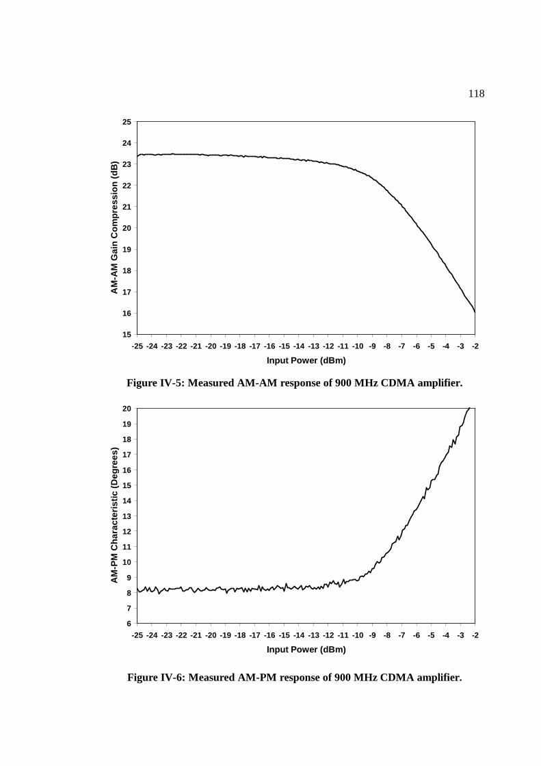
118
15
16
17
18
19
20
21
22
23
24
25
-25 -24 -23 -22 -21 -20 -19 -18 -17 -16 -15 -14 -13 -12 -11 -10 -9 -8 -7 -6 -5 -4 -3 -2
Input Power (dBm)
AM
-AM
Gai
n C
om
pre
ssio
n (
dB
)
Figure IV-5: Measured AM-AM response of 900 MHz CDMA amplifier.
6
7
8
9
10
11
12
13
14
15
16
17
18
19
20
-25 -24 -23 -22 -21 -20 -19 -18 -17 -16 -15 -14 -13 -12 -11 -10 -9 -8 -7 -6 -5 -4 -3 -2
Input Power (dBm)
AM
-PM
Ch
arac
teri
stic
(D
egre
es)
Figure IV-6: Measured AM-PM response of 900 MHz CDMA amplifier.

119
Modern RFIC integrated heterodyne and direct conversion transmitter circuits [91-
96] pose an interesting challenge for measurement of AM-AM and AM-PM
characteristics because the input is a quadrature baseband signal and the output is a RF
signal. Block diagrams of a superheterodyne and direct conversion RFIC devices are
shown in A simple solution is to sweep a DC offset at the in-phase and quadrature
inputs of the device thus generating carrier feedthrough which is proportional to the
DC offset at the input. The input DC offset is swept from the fullscale input value
down to a reasonable level to achieve a linear gain and phase measurement. Gain and
phase are determined by comparing the output carrier feedthrough to a fixed reference
source using a vector voltmeter. An example measurement setup is shown in Figure
IV-8. The input signal is controlled by an arbitrary waveform generator which accepts
digital inputs from a computer and generates an analog output signal. Additional
sinusoidal signal generators are required to present local oscillator (LO) signals which
are phase locked to the same PLL reference signal to insure a stable phase comparison
measurement against the reference signal generator.
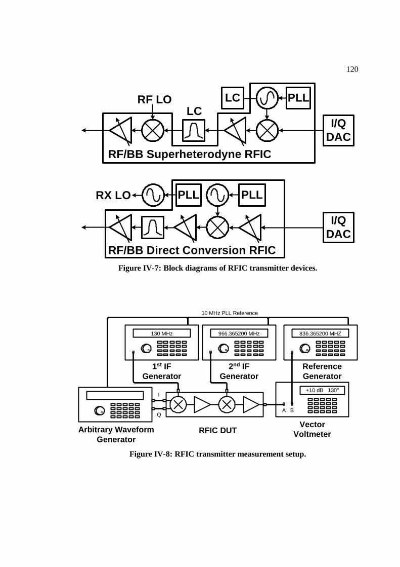
120
I/QDAC
RF/BB Superheterodyne RFIC
RF/BB Direct Conversion RFIC
PLL
PLL
RF LO
PLLRX LO
LCLC
I/QDAC
Figure IV-7: Block diagrams of RFIC transmitter devices.
+10 dB 130°
966.365200 MHz 836.365200 MHZ
A B
ReferenceGenerator
2nd IFGenerator
VectorVoltmeter
130 MHz
1st IFGenerator
10 MHz PLL Reference
Arbitrary WaveformGenerator
I
Q
RFIC DUT
Figure IV-8: RFIC transmitter measurement setup.

121
One drawback of using a swept DC input offset signal is the finite carrier
suppression of the RFIC DUT will limit the lower bound on the linear gain
measurement. Carrier suppression in the DUT is determined by mismatches between
devices and layout imbalances in the circuits internal to the DUT. As the input DC
offset is reduced the finite carrier suppression starts to contribute to the output signal
resulting in an apparent increase in gain because the output signal is not dropping in
relation to the input signal. One solution for overcoming this limitation is to use a
quadrature sinusoidal input signal instead of a DC offset. A single sideband signal is
generated which is offset to the carrier; thus, the amplitude of the sinusoid can be
measured at levels lower than the carrier feedthrough. However, this measurement
technique requires that the input signal is also carefully locked to the same PLL
reference signal as the LO and reference signal generators in order to make a stable
phase comparison measurement.
The RFIC setup shown in Figure IV-8 was used to measure the AM-AM and AM-
PM characteristics of a superheterodyne [95] and a direct conversion [91] dual band
CDMA transmitter devices. The superheterodyne RFIC requires the use of two LO
signal generators: one for the conversion from baseband to the first intermediate
frequency (IF) and a second IF LO to upconvert from IF to the RF output frequency.
The input DC offset was swept over a 40 dB range referenced to the full scale input
signal value. The RFIC supports over 90 dB of dynamic gain control range; however,
ACPR performance is typically worst at the maximum rated output power.
Accordingly, the gain control settings required to achieve rated output power values
are determined before making the AM-AM and AM-PM measurements. The measured
AM-AM and AM-PM characteristics for the superheterodyne RFIC operating in the
cell band at 8.3 dBm CDMA output power and PCS band at 9.7 dBm CDMA output
power are shown in Figure IV-9 and Figure IV-10 respectively.

122
Measurement of the direct conversion device requires only one LO generator to
support the upconversion mixer. The measured AM-AM and AM-PM characteristics
for the direct conversion RFIC operating in the cell band at 8.0 dBm CDMA output
power and PCS band at 10.0 dBm CDMA output power are shown in Figure IV-11
and Figure IV-12 respectively. Carrier suppression performance for the
superheterodyne transmitter is better than the direct conversion design because only the
first IF upconversion stage, operating at 130 MHz, contributes to the carrier
feedthrough. The direct conversion transmitter mixer operates at the RF output
frequency which is more susceptible to carrier leakage due to stray capacitance and
substrate coupling providing paths for the LO signal to leak around the mixer stage.
The effects of carrier leakage are apparent in both the AM-AM and AM-PM plots
below -25 dB baseband signal level for the direct conversion device.

123
73.5
74.0
74.5
75.0
75.5
76.0
76.5
77.0
-40 -35 -30 -25 -20 -15 -10 -5 0
Baseband Input Level (dB)
Gai
n (d
B)
122
124
126
128
130
132
134
136
Ph
ase
(deg
ree)
Figure IV-9: Cell band AM-AM AM-PM for superheterodyne RFIC.
70.2
70.4
70.6
70.8
71.0
71.2
71.4
71.6
71.8
72.0
72.2
72.4
72.6
-40 -35 -30 -25 -20 -15 -10 -5 0
Baseband Input Level (dB)
Gai
n (
dB
)
-84
-82
-80
-78
-76
-74
-72
-70
-68
-66
-64
-62
-60
Ph
ase
(deg
ree)
Figure IV-10: PCS band AM-AM AM-PM for superheterodyne RFIC.

124
75.0
75.5
76.0
76.5
77.0
77.5
78.0
78.5
79.0
79.5
80.0
-40 -35 -30 -25 -20 -15 -10 -5 0
Baseband Input Level (dB)
Gai
n (
dB
)
-72
-70
-68
-66
-64
-62
-60
-58
-56
-54
-52
Ph
ase
(deg
ree)
Figure IV-11: Cell band AM-AM AM-PM for direct conversion RFIC.
77.0
77.5
78.0
78.5
79.0
79.5
80.0
80.5
81.0
81.5
82.0
-40 -35 -30 -25 -20 -15 -10 -5 0
Baseband Input Level (dB)
Gai
n (
dB
)
-120
-115
-110
-105
-100
-95
-90
-85
-80
-75
-70
Ph
ase
(deg
ree)
Figure IV-12: PCS band AM-AM AM-PM for direct conversion RFIC.

125
IV.3 ACPR Measurements
The general time average autocorrelation function and the complex Gaussian
moment methods were used to calculate the output power spectrum and ACPR of an
integrated RF amplifier with CDMA and complex Gaussian input signals. The amplifier
is the GaAs MESFET 900MHz driver amplifer described in section IV.2 [62]. The
AM-AM, AM-PM characteristics from Figure IV-5 and Figure IV-6 were fit to a
complex power series of odd order N=13 using a least squares solution to the over
determined system of equations as described in section II.6. The resulting complex
power series coefficients are shown in Table IV-1 and a plot of the power series model
and measured data are shown in Figure IV-13.
Table IV-1: Complex power series coefficients for 900 MHz CDMA amplifier.
Term Units Real Coefficient Imaginary Coefficient
1aɶ 1 1.47437438509120E+01 2.13403737823950E+00
3aɶ 2v− -6.70889896661973E+01 -2.06242049102448E+01
5aɶ 4v− -6.34509397147117E+03 2.64680409468526E+03
7aɶ 6v− -2.02512977741845E+05 -5.02911140999704E+04
9aɶ 8v− 1.72980263843510E+07 -1.04643833028688E+06
11aɶ 10v− -3.28432949645493E+08 3.76656913802756E+07
13aɶ 12v− 1.99599335429889E+09 -2.78828805740329E+08

126
15
16
17
18
19
20
21
22
23
24
-24 -22 -20 -18 -16 -14 -12 -10 -8 -6 -4 -2
Input Power (dBm)
AM
-AM
Gai
n (
dB
)
-174
-172
-170
-168
-166
-164
-162
-160
-158
-156
AM
-PM
Ph
ase
(Deg
rees
)
MODELED
MEASURED
Figure IV-13: Modeled and measured AM-AM/AM-PM for CDMA amplifier.
A carrier modulated with a IS-95 CDMA reverse link signal is applied to the
amplifier circuit and the output distortion measured using a spectrum analyzer.
Specifically, an Agilent ESG series signal generator with the capability to generate a
IS-95 CDMA signal was used as the signal source and an Agilent vector signal analyzer
(VSA) was used to measure the adjacent channel power ratio (ACPR) is the standard
distortion measurement for CDMA transmitters. The VSA equipment has built in
measurement routines to measure ACPR for specified offsets to the carrier frequency.
ACPR is the ratio, in decibels, of the distortion power, in a 30 kHz bandwidth offset by
±885 kHz, and the desired channel power, in a 1.23MHz bandwidth as defined in the
IS-95 standard [2]. The measured ACPR is shown in Figure IV-14. The ACPR was
calculated using the general time average correlation function formulation presented in
Chapter I and the power series coefficients from Table IV-1. The simulated ACPR
results using the composite of the gain compression/expansion (II.26) and distortion

127
terms (II.27) agree well with the measured data shown in Figure IV-14. The ACPR
plateaus at lower output power because of the finite rejection of the CDMA baseband
filter used by the waveform generator.
-65
-60
-55
-50
-45
-40
-35
-30
-25
-20
-15
-2 -1 0 1 2 3 4 5 6 7 8 9 10 11 12 13
Output Power (dBm)
AC
PR
(d
Bc)
Measured ACPR
Time Average Autocorrelation Formulation
Figure IV-14: Measured and calculated ACPR for CDMA reverse link signal.
A complex Gaussian signal was also used to measure ACPR, using the IS-95
definition, to compare against both the complex Gaussian moment and the time average
autocorrelation formulations. The Agilent ESG signal generator is capable of
generating a complex Gaussian signal filtered with a finite impulse response (FIR) filter
with a maximally flat response. The ACPR measurements along with the predicted
ACPR from both the complex Gaussian moment and time average autocorrelation
formulations are shown in Figure IV-15. The measured and predicted ACPR are in
good agreement below an output power level of 11 dBm. Both the complex Gaussian
moment and time average autocorrelation formulations deviate from the measured data
because of the limited dynamic range of the complex power series model of the

128
nonlinear amplifier. The difference in dynamic range between using the CDMA and
complex Gaussian input signals is approximately 2 dB which is consistent with
differences found with the hyperbolic tangent limiter model when comparing Figure
II-20 and Figure III-4. -65
-60
-55
-50
-45
-40
-35
-30
-25
-20
-15
-10
-2 -1 0 1 2 3 4 5 6 7 8 9 10 11 12 13
Output Power (dBm)
AC
PR
(d
Bc)
Measured Complex Gaussian
Complex Gaussian Moment Formulation
Time Average Autocorrelation Formulation
Figure IV-15: Measured and calculated ACPR for complex Gaussian input signal.
IV.4 Summary
This chapter presented the results of comparing the time average autocorrelation
and complex Gaussian moment formulations against a commercial transient envelope
simulation tool and measurements from an integrated CDMA amplifier. Comparisons
with a commercial simulator verify the equivalence of the time average autocorrelation
and complex Gaussian moment formulations with time domain solutions using a
Fourier transform to obtain the power spectrum. The time average autocorrelation and
complex Gaussian moment calculations provide a significant advantage in the processor

129
time and data storage required to perform a power sweep analysis of ACPR.
Although, equivalent usage of autocorrelation methods, during the design phase of a
wireless circuit, requires single tone power sweep simulations to generate the AM-AM
and AM-PM characteristics. An added benefit of this procedure is that the power
spectrum or distortion characteristics caused by different input signals can be
determined quickly once the AM-AM and AM-PM characteristics are extracted.
Comparisons of the time average autocorrelation and complex Gaussian moment
formulations with measured ACPR data from a CDMA amplifier validate the
techniques when used with real data from an actual nonlinear wireless amplifier. Thus
the techniques described can be used during the design phase with simulated AM-AM
and AM-PM characteristics or during the characterization phase with measured data.
The text of this chapter, in part, is a reprint of the material as it appears in our
published papers in IEEE Conferences [RAWCON03, CICC01, and IMS01] and
publication in IEEE Transactions on Microwave Theory and Techniques [1999 and
submitted 2003]. The dissertation author was the primary investigator and author of
these papers.

130
V. Conclusions
Two methods for analyzing the power spectrum of modulated carriers passed
through a nonlinear wireless circuit were presented. The first method is based on
formulating the time average autocorrelation function for a signal passed through a
complex power series behavioral model of the AM-AM and AM-PM characteristics of
a wireless amplifier. The power spectrum of the signal is obtained via the Fourier
transformation of the output autocorrelation function leading to a summation of
[ ]2( 1) / 2N − for a Nth odd order power series expansion of the nonlinearity. The second
method is based on a transformation of the statistical properties of the modulated
carrier passed through a nonlinear amplifier. The second order moments of the
nonlinear terms are calculated and combined leading to a closed form expression of the
output autocorrelation in terms of the autocorrelation function of the input signal. The
statistical formulation yields ( 1) / 2N − spectral terms for real and complex Gaussian
modulation of the carrier. Thus there is a significant reduction in the number of
spectral terms compared to the time average autocorrelation formulation. Both
analysis techniques were applied to limiter amplifier models and demonstrated excellent
agreement when compared against measured data from a CDMA amplifier.
Autocorrelation analysis of the output power spectrum also provides improvements
in speed of calculating the output power spectrum of a signal passed through a
nonlinear circuit. The autocorrelation formulation permits precalculation of all spectral
terms such that the only calculations required are multiplication of each spectral term
by the appropriate complex power series coefficients and input power scaling factor.
V.1 Future Work
The work presented in this dissertation establishes a foundation for analyzing
problems involving modulated carrier signals passed through nonlinear circuits. The

131
motivation of this work is to provide circuit designers with an efficient tool that
provides insight into the interactions between signals and nonlinear circuits. Likewise,
this work can also be used by wireless system designers to better understand the impact
of nonlinear channels on system performance. Thus the modeling and analysis
techniques presented bring circuit and system designers closer to understanding the
impact of nonlinear circuits used in wireless communication systems. Future
contributions to this work should focus on improving the modeling techniques to
incorporate behavior not accounted for in the bandpass nonlinearity assumption and to
apply the analysis techniques to communication system performance analysis. Future
work is divided into three primary areas: distortion analysis, wireless system analysis,
and behavioral modeling of nonlinear circuits.
V.1.1 Distortion Analysis
The bandpass nonlinearity formulations from focus on distortion generated by one
modulated carrier passed through a nonlinear circuit; however, there are practical
design problems which involve two or more modulated carriers passed through a
common nonlinearity. Such is the case for cable and satellite systems where many
modulated carriers are passed through a hybrid amplifier, traveling wave tube amplifier,
or a fiber optic link. The multi-carrier problem was introduced with the bandpass
nonlinearity crossmodulation analysis presented in chapter II. Another practical
problem is a phenomenon which causes asymmetry in the ACPR distortion response
where one distortion sideband is higher in amplitude than the other. The asymmetry is
attributed to second-order interaction terms, which end up at baseband, interacting with
the baseband frequency response of the bias circuits controlling the input impedance
high frequency amplifiers and mixers.

132
V.1.2 Wireless System Analysis
Wireless communication systems are becoming increasingly complex to provide
greater capacity and bandwidth to support more users and provide high data rate
mobile services for customers. As the systems advance, the modulation schemes also
grow in complexity by adding additional code channels. Interaction between the
multiple code channels when passed through a nonlinear channel is not well
understood. The Gaussian random variable analysis presented in chapter III is crudely
related to the case of multiple code channels; however, the analysis doesn’t separate the
impact of the distortion as it relates to the SNR of an individual code channel. Bit error
rate (BER) is a popular figure of merit for communication system performance;
although, frame error rate (FER) is gaining popularity since it more directly relates to
average throughput rates than BER. Both the general time average autocorrelation
function and the Gaussian moment analysis could be applied to accessing the
degradation in SNR when a signal is passed through a nonlinear channel. The SNR
results could then be related to BER or FER.
V.1.3 Behavioral Modeling
The bandpass nonlinearity model accommodates a wide range of circuit
applications; however, there are limitations which prevent accurate representation of
physical phenomena observed when a modulated carrier is passed through a nonlinear
circuit. The primary deficiency is that frequency dependency of the distortion is not
modeled by the memoryless nonlinearity assumption. For instance, asymmetry in the
distortion sidebands is commonly observed in commercial class AB amplifiers. The
asymmetry in the intermodulation distortion is typically associated second-order
interaction terms that are influenced by the low frequency impedance of bias circuits.
One possible solution is to augment the bandpass nonlinearity model with second-order

133
interact terms filter by a low-pass filter to model the baseband frequency dependencies.
Such a model also requires more sophisticated measurement techniques to characterize
the frequency dependent asymmetric intermodulation response.
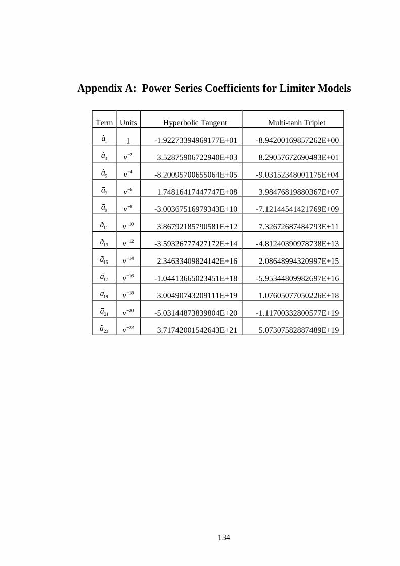
134
Appendix A: Power Series Coefficients for Limiter Models
Term Units Hyperbolic Tangent Multi-tanh Triplet
1aɶ 1 -1.92273394969177E+01 -8.94200169857262E+00
3aɶ 2v− 3.52875906722940E+03 8.29057672690493E+01
5aɶ 4v− -8.20095700655064E+05 -9.03152348001175E+04
7aɶ 6v− 1.74816417447747E+08 3.98476819880367E+07
9aɶ 8v− -3.00367516979343E+10 -7.12144541421769E+09
11aɶ 10v− 3.86792185790581E+12 7.32672687484793E+11
13aɶ 12v− -3.59326777427172E+14 -4.81240390978738E+13
15aɶ 14v− 2.34633409824142E+16 2.08648994320997E+15
17aɶ 16v− -1.04413665023451E+18 -5.95344809982697E+16
19aɶ 18v− 3.00490743209111E+19 1.07605077050226E+18
21aɶ 20v− -5.03144873839804E+20 -1.11700332800577E+19
23aɶ 22v− 3.71742001542643E+21 5.07307582887489E+19

135
Term Units Cann s=2 Cann s=4
1aɶ 1 -1.92156104076352E+01 -1.92483328748561E+01
3aɶ 2v− 5.17085137414416E+03 -1.59477825294859E+01
5aɶ 4v− -1.99651515752524E+06 2.14927531339979E+06
7aɶ 6v− 6.68485061979126E+08 -1.01623225111983E+09
9aɶ 8v− -1.66402682205888E+11 2.55711246566700E+11
11aɶ 10v− 2.92812854236135E+13 -4.04429693977267E+13
13aɶ 12v− -3.58277052876239E+15 4.23264309379138E+15
15aɶ 14v− 3.01050436899200E+17 -2.97372848039920E+17
17aɶ 16v− -1.69747749907222E+19 1.38705628275514E+19
19aɶ 18v− 6.12183400679467E+20 -4.11849587901765E+20
21aɶ 20v− -1.27374980795224E+22 7.04408220380322E+21
23aɶ 22v− 1.16142923340519E+23 -5.28103013086195E+22

136
Term Units Cann s=10 Cann s=100
1aɶ 1 -1.92535703079452E+01 -1.93042722589944E+01
3aɶ 2v− 6.39247187051352E+02 5.66417493276341E+02
5aɶ 4v− -2.82229340562232E+06 5.06025737179413E+05
7aɶ 6v− 4.02352004775739E+09 -5.27432803014226E+09
9aɶ 8v− -2.16096223123555E+12 7.57850716050558E+12
11aɶ 10v− 6.40179065754809E+14 -4.73485765216818E+15
13aɶ 12v− -1.17804804114307E+17 1.65770382995701E+18
15aɶ 14v− 1.40541137652110E+19 -3.55956344326610E+20
17aɶ 16v− -1.09013826245762E+21 4.80529966859682E+22
19aɶ 18v− 5.31192610999943E+22 -3.98644568685045E+24
21aɶ 20v− -1.47785861518937E+24 1.85982481756989E+26
23aɶ 22v− 1.79134069101052E+25 -3.73928861382277E+27

137
Appendix B: MATLAB Code
CDMA/Gaussian Waveform Generator MATLAB Code % This program creates an IS-95 OQPSK waveform of n symbols and % estimates an autocorrelation function, Rxy, and n th order odd % power spectrum up to order 11. Rxy and the power spectrums are % normalized to 0dBm, so that scaling is easily han dled by weighting % the power spectrum by 10^(dBm/10) where dBm is th e desired power % in dBm. % This program reads in one file containing the bas eband FIR filter % coeffecients % % Kevin Gard % % Load CDMA FIR filter coefficients load cdma141.txt; is95taps=cdma141; % Set the number of symbols m=256; % m are excess symbols for initializing the FIR filter n=(2^16)+m; % Generate hard limited Gaussian samples bitsI=sign(randn(n,1)); bitsQ=sign(randn(n,1)); chipbitsI=zeros(4*n,1); chipbitsQ=chipbitsI; chipbitsO_Q=chipbitsI; lchip=1:n; % Insert zeros for 4x oversampling with (1 bit 3 ze ros) chipbitsI((lchip-1)*4+1)=bitsI(lchip); chipbitsO_Q((lchip-1)*4+3)=bitsQ(lchip); chipbitsQ((lchip-1)*4+1)=bitsQ(lchip); % Filter the I and Q data with FIR filter Ichan=filter(is95taps,1,chipbitsI); clear chipbitsI %Qchan=filter(is95taps,1,chipbitsQ); %clear chipbisQ O_Qchan=filter(is95taps,1,chipbitsQ); clear chipbitsQ % Ideal interpolation from 4x to 8x oversampling p=2; Ichan=interp(Ichan,p); O_Qchan=interp(O_Qchan,p); % Add I and Q in quadrature and scale final signal to 0dBm power Pin=10*log10(mean(abs(Ichan(4*p*m+1:p*4*n)+j*O_Qcha n(4*p*m+1:p*4*n)).^2)/(50*.001)); Pscale=10^(Pin/10); CDMA_O=sqrt(1/Pscale)*(Ichan(4*p*m+1:p*4*n)+j*O_Qch an(4*p*m+1:p*4*n)); xr=real(CDMA_O); xi=imag(CDMA_O); % Save waveform to text file save cdma_wav_141_8x_16 CDMA_O

138
Autocorrelation and Spectral File Generator MATLAB Code % This program generates all spectral terms necessa ry for % calculating ACPR from a power series nonlinearity . % An input time domain waveform file is read in the n all autocorrelation % terms up to order N=23, 144 terms, are calculated . The spectral terms are then calculated % from the FFT of the autocorrelation terms. % % ***WARNING*** % This program requires at least 128MB of available RAM and can take quite a while % to complete (10 minutes on a P4) depending on the size of the input waveform. % % Load input waveform file (I/Q data in two columns ) % The matlab file cdma_file_gen.m can be used to ge nerate waveform textfile. t0 = clock; load cdma_qpsk_wav_141_8x_16; n=length(CDMA_O); % Set the number of autocorrelation lags y=2^11; % Compute the autocorrelation estimate cx=CDMA_O; cjx=conj(CDMA_O); cy=cx.*cjx; r11=xcorr(cx,cx,y,'biased'); r13=xcorr(cx,conj(cx.*cjx.^2),y,'biased'); r31=xcorr(cx.^2.*cjx,conj(cjx),y,'biased'); r33=xcorr(cx.^2.*cjx,conj(cx.*cjx.^2),y,'biased'); r15=xcorr(cx,conj(cx.^2.*cjx.^3),y,'biased'); r51=xcorr(cx.^3.*cjx.^2,conj(cjx),y,'biased'); r35=xcorr(cx.^2.*cjx,conj(cx.^2.*cjx.^3),y,'biased' ); r53=xcorr(cx.^3.*cjx.^2,conj(cx.*cjx.^2),y,'biased' ); r55=xcorr(cx.^3.*cjx.^2,conj(cx.^2.*cjx.^3),y,'bias ed'); r17=xcorr(cx,conj(cx.^3.*cjx.^4),y,'biased'); r71=xcorr(cx.^4.*cjx.^3,conj(cjx),y,'biased'); r37=xcorr(cx.^2.*cjx,conj(cx.^3.*cjx.^4),y,'biased' ); r73=xcorr(cx.^4.*cjx.^3,conj(cx.*cjx.^2),y,'biased' ); r57=xcorr(cx.^3.*cjx.^2,conj(cx.^3.*cjx.^4),y,'bias ed'); r75=xcorr(cx.^4.*cjx.^3,conj(cx.^2.*cjx.^3),y,'bias ed'); r77=xcorr(cx.^4.*cjx.^3,conj(cx.^3.*cjx.^4),y,'bias ed'); r19=xcorr(cx,conj(cx.^4.*cjx.^5),y,'biased'); r91=xcorr(cx.^5.*cjx.^4,conj(cjx),y,'biased'); r39=xcorr(cx.^2.*cjx,conj(cx.^4.*cjx.^5),y,'biased' ); r93=xcorr(cx.^5.*cjx.^4,conj(cx.*cjx.^2),y,'biased' ); r59=xcorr(cx.^3.*cjx.^2,conj(cx.^4.*cjx.^5),y,'bias ed'); r95=xcorr(cx.^5.*cjx.^4,conj(cx.^2.*cjx.^3),y,'bias ed'); r79=xcorr(cx.^4.*cjx.^3,conj(cx.^4.*cjx.^5),y,'bias ed'); r97=xcorr(cx.^5.*cjx.^4,conj(cx.^3.*cjx.^4),y,'bias ed'); r99=xcorr(cx.^5.*cjx.^4,conj(cx.^4.*cjx.^5),y,'bias ed'); r1_11=xcorr(cx,conj(cx.^5.*cjx.^6),y,'biased'); r11_1=xcorr(cx.^6.*cjx.^5,conj(cjx),y,'biased'); r311=xcorr(cx.^2.*cjx,conj(cx.^5.*cjx.^6),y,'biased '); r113=xcorr(cx.^6.*cjx.^5,conj(cx.*cjx.^2),y,'biased '); r511=xcorr(cx.^3.*cjx.^2,conj(cx.^5.*cjx.^6),y,'bia sed'); r115=xcorr(cx.^6.*cjx.^5,conj(cx.^2.*cjx.^3),y,'bia sed'); r711=xcorr(cx.^4.*cjx.^3,conj(cx.^5.*cjx.^6),y,'bia sed'); r117=xcorr(cx.^6.*cjx.^5,conj(cx.^3.*cjx.^4),y,'bia sed'); r911=xcorr(cx.^5.*cjx.^4,conj(cx.^5.*cjx.^6),y,'bia sed'); r119=xcorr(cx.^6.*cjx.^5,conj(cx.^4.*cjx.^5),y,'bia sed'); r1111=xcorr(cx.^6.*cjx.^5,conj(cx.^5.*cjx.^6),y,'bi ased'); r1_13=xcorr(cx,conj(cx.^6.*cjx.^7),y,'biased'); r13_1=xcorr(cx.^7.*cjx.^6,conj(cjx),y,'biased'); r3_13=xcorr(cx.^2.*cjx,conj(cx.^6.*cjx.^7),y,'biase d'); r13_3=xcorr(cx.^7.*cjx.^6,conj(cx.*cjx.^2),y,'biase d'); r513=xcorr(cx.^3.*cjx.^2,conj(cx.^6.*cjx.^7),y,'bia sed'); r135=xcorr(cx.^7.*cjx.^6,conj(cx.^2.*cjx.^3),y,'bia sed'); r713=xcorr(cx.^4.*cjx.^3,conj(cx.^6.*cjx.^7),y,'bia sed'); r137=xcorr(cx.^7.*cjx.^6,conj(cx.^3.*cjx.^4),y,'bia sed'); r913=xcorr(cx.^5.*cjx.^4,conj(cx.^6.*cjx.^7),y,'bia sed'); r139=xcorr(cx.^7.*cjx.^6,conj(cx.^4.*cjx.^5),y,'bia sed'); r1113=xcorr(cx.^6.*cjx.^5,conj(cx.^6.*cjx.^7),y,'bi ased'); r1311=xcorr(cx.^7.*cjx.^6,conj(cx.^5.*cjx.^6),y,'bi ased');

139
r1313=xcorr(cx.^7.*cjx.^6,conj(cx.^6.*cjx.^7),y,'bi ased'); r1_15=xcorr(cx,conj(cx.^7.*cjx.^8),y,'biased'); r15_1=xcorr(cx.^8.*cjx.^7,conj(cjx),y,'biased'); r3_15=xcorr(cx.^2.*cjx,conj(cx.^7.*cjx.^8),y,'biase d'); r15_3=xcorr(cx.^8.*cjx.^7,conj(cx.*cjx.^2),y,'biase d'); r515=xcorr(cx.^3.*cjx.^2,conj(cx.^7.*cjx.^8),y,'bia sed'); r155=xcorr(cx.^8.*cjx.^7,conj(cx.^2.*cjx.^3),y,'bia sed'); r715=xcorr(cx.^4.*cjx.^3,conj(cx.^7.*cjx.^8),y,'bia sed'); r157=xcorr(cx.^8.*cjx.^7,conj(cx.^3.*cjx.^4),y,'bia sed'); r915=xcorr(cx.^5.*cjx.^4,conj(cx.^7.*cjx.^8),y,'bia sed'); r159=xcorr(cx.^8.*cjx.^7,conj(cx.^4.*cjx.^5),y,'bia sed'); r1115=xcorr(cx.^6.*cjx.^5,conj(cx.^7.*cjx.^8),y,'bi ased'); r1511=xcorr(cx.^8.*cjx.^7,conj(cx.^5.*cjx.^6),y,'bi ased'); r1315=xcorr(cx.^7.*cjx.^6,conj(cx.^7.*cjx.^8),y,'bi ased'); r1513=xcorr(cx.^8.*cjx.^7,conj(cx.^6.*cjx.^7),y,'bi ased'); r1515=xcorr(cx.^8.*cjx.^7,conj(cx.^7.*cjx.^8),y,'bi ased'); r1_17=xcorr(cx,conj(cx.^8.*cjx.^9),y,'biased'); r17_1=xcorr(cx.^9.*cjx.^8,conj(cjx),y,'biased'); r3_17=xcorr(cx.^2.*cjx,conj(cx.^8.*cjx.^9),y,'biase d'); r17_3=xcorr(cx.^9.*cjx.^8,conj(cx.*cjx.^2),y,'biase d'); r517=xcorr(cx.^3.*cjx.^2,conj(cx.^8.*cjx.^9),y,'bia sed'); r175=xcorr(cx.^9.*cjx.^8,conj(cx.^2.*cjx.^3),y,'bia sed'); r717=xcorr(cx.^4.*cjx.^3,conj(cx.^8.*cjx.^9),y,'bia sed'); r177=xcorr(cx.^9.*cjx.^8,conj(cx.^3.*cjx.^4),y,'bia sed'); r917=xcorr(cx.^5.*cjx.^4,conj(cx.^8.*cjx.^9),y,'bia sed'); r179=xcorr(cx.^9.*cjx.^8,conj(cx.^4.*cjx.^5),y,'bia sed'); r1117=xcorr(cx.^6.*cjx.^5,conj(cx.^8.*cjx.^9),y,'bi ased'); r1711=xcorr(cx.^9.*cjx.^8,conj(cx.^5.*cjx.^6),y,'bi ased'); r1317=xcorr(cx.^7.*cjx.^6,conj(cx.^8.*cjx.^9),y,'bi ased'); r1713=xcorr(cx.^9.*cjx.^8,conj(cx.^6.*cjx.^7),y,'bi ased'); r1517=xcorr(cx.^8.*cjx.^7,conj(cx.^8.*cjx.^9),y,'bi ased'); r1715=xcorr(cx.^9.*cjx.^8,conj(cx.^7.*cjx.^8),y,'bi ased'); r1717=xcorr(cx.^9.*cjx.^8,conj(cx.^8.*cjx.^9),y,'bi ased'); r1_19=xcorr(cx,conj(cx.^9.*cjx.^10),y,'biased'); r19_1=xcorr(cx.^10.*cjx.^9,conj(cjx),y,'biased'); r3_19=xcorr(cx.^2.*cjx,conj(cx.^9.*cjx.^10),y,'bias ed'); r19_3=xcorr(cx.^10.*cjx.^9,conj(cx.*cjx.^2),y,'bias ed'); r519=xcorr(cx.^3.*cjx.^2,conj(cx.^9.*cjx.^10),y,'bi ased'); r195=xcorr(cx.^10.*cjx.^9,conj(cx.^2.*cjx.^3),y,'bi ased'); r719=xcorr(cx.^4.*cjx.^3,conj(cx.^9.*cjx.^10),y,'bi ased'); r197=xcorr(cx.^10.*cjx.^9,conj(cx.^3.*cjx.^4),y,'bi ased'); r919=xcorr(cx.^5.*cjx.^4,conj(cx.^9.*cjx.^10),y,'bi ased'); r199=xcorr(cx.^10.*cjx.^9,conj(cx.^4.*cjx.^5),y,'bi ased'); r1119=xcorr(cx.^6.*cjx.^5,conj(cx.^9.*cjx.^10),y,'b iased'); r1911=xcorr(cx.^10.*cjx.^9,conj(cx.^5.*cjx.^6),y,'b iased'); r1319=xcorr(cx.^7.*cjx.^6,conj(cx.^9.*cjx.^10),y,'b iased'); r1913=xcorr(cx.^10.*cjx.^9,conj(cx.^6.*cjx.^7),y,'b iased'); r1519=xcorr(cx.^8.*cjx.^7,conj(cx.^9.*cjx.^10),y,'b iased'); r1915=xcorr(cx.^10.*cjx.^9,conj(cx.^7.*cjx.^8),y,'b iased'); r1719=xcorr(cx.^9.*cjx.^8,conj(cx.^9.*cjx.^10),y,'b iased'); r1917=xcorr(cx.^10.*cjx.^9,conj(cx.^8.*cjx.^9),y,'b iased'); r1919=xcorr(cx.^10.*cjx.^9,conj(cx.^9.*cjx.^10),y,' biased'); r1_21=xcorr(cx,conj(cx.^10.*cjx.^11),y,'biased'); r21_1=xcorr(cx.^11.*cjx.^10,conj(cjx),y,'biased'); r3_21=xcorr(cx.^2.*cjx,conj(cx.^10.*cjx.^11),y,'bia sed'); r21_3=xcorr(cx.^11.*cjx.^10,conj(cx.*cjx.^2),y,'bia sed'); r521=xcorr(cx.^3.*cjx.^2,conj(cx.^10.*cjx.^11),y,'b iased'); r215=xcorr(cx.^11.*cjx.^10,conj(cx.^2.*cjx.^3),y,'b iased'); r721=xcorr(cx.^4.*cjx.^3,conj(cx.^10.*cjx.^11),y,'b iased'); r217=xcorr(cx.^11.*cjx.^10,conj(cx.^3.*cjx.^4),y,'b iased'); r921=xcorr(cx.^5.*cjx.^4,conj(cx.^10.*cjx.^11),y,'b iased'); r219=xcorr(cx.^11.*cjx.^10,conj(cx.^4.*cjx.^5),y,'b iased'); r1121=xcorr(cx.^6.*cjx.^5,conj(cx.^10.*cjx.^11),y,' biased'); r2111=xcorr(cx.^11.*cjx.^10,conj(cx.^5.*cjx.^6),y,' biased'); r1321=xcorr(cx.^7.*cjx.^6,conj(cx.^10.*cjx.^11),y,' biased'); r2113=xcorr(cx.^11.*cjx.^10,conj(cx.^6.*cjx.^7),y,' biased'); r1521=xcorr(cx.^8.*cjx.^7,conj(cx.^10.*cjx.^11),y,' biased'); r2115=xcorr(cx.^11.*cjx.^10,conj(cx.^7.*cjx.^8),y,' biased'); r1721=xcorr(cx.^9.*cjx.^8,conj(cx.^10.*cjx.^11),y,' biased'); r2117=xcorr(cx.^11.*cjx.^10,conj(cx.^8.*cjx.^9),y,' biased'); r1921=xcorr(cx.^10.*cjx.^9,conj(cx.^10.*cjx.^11),y, 'biased'); r2119=xcorr(cx.^11.*cjx.^10,conj(cx.^9.*cjx.^10),y, 'biased');

140
r2121=xcorr(cx.^11.*cjx.^10,conj(cx.^10.*cjx.^11),y ,'biased'); r1_23=xcorr(cx,conj(cx.^11.*cjx.^12),y,'biased'); r23_1=xcorr(cx.^12.*cjx.^11,conj(cjx),y,'biased'); r3_23=xcorr(cx.^2.*cjx,conj(cx.^11.*cjx.^12),y,'bia sed'); r23_3=xcorr(cx.^12.*cjx.^11,conj(cx.*cjx.^2),y,'bia sed'); r523=xcorr(cx.^3.*cjx.^2,conj(cx.^11.*cjx.^12),y,'b iased'); r235=xcorr(cx.^12.*cjx.^11,conj(cx.^2.*cjx.^3),y,'b iased'); r723=xcorr(cx.^4.*cjx.^3,conj(cx.^11.*cjx.^12),y,'b iased'); r237=xcorr(cx.^12.*cjx.^11,conj(cx.^3.*cjx.^4),y,'b iased'); r923=xcorr(cx.^5.*cjx.^4,conj(cx.^11.*cjx.^12),y,'b iased'); r239=xcorr(cx.^12.*cjx.^11,conj(cx.^4.*cjx.^5),y,'b iased'); r1123=xcorr(cx.^6.*cjx.^5,conj(cx.^11.*cjx.^12),y,' biased'); r2311=xcorr(cx.^12.*cjx.^11,conj(cx.^5.*cjx.^6),y,' biased'); r1323=xcorr(cx.^7.*cjx.^6,conj(cx.^11.*cjx.^12),y,' biased'); r2313=xcorr(cx.^12.*cjx.^11,conj(cx.^6.*cjx.^7),y,' biased'); r1523=xcorr(cx.^8.*cjx.^7,conj(cx.^11.*cjx.^12),y,' biased'); r2315=xcorr(cx.^12.*cjx.^11,conj(cx.^7.*cjx.^8),y,' biased'); r1723=xcorr(cx.^9.*cjx.^8,conj(cx.^11.*cjx.^12),y,' biased'); r2317=xcorr(cx.^12.*cjx.^11,conj(cx.^8.*cjx.^9),y,' biased'); r1923=xcorr(cx.^10.*cjx.^9,conj(cx.^11.*cjx.^12),y, 'biased'); r2319=xcorr(cx.^12.*cjx.^11,conj(cx.^9.*cjx.^10),y, 'biased'); r2123=xcorr(cx.^11.*cjx.^10,conj(cx.^11.*cjx.^12),y ,'biased'); r2321=xcorr(cx.^12.*cjx.^11,conj(cx.^10.*cjx.^11),y ,'biased'); r2323=xcorr(cx.^12.*cjx.^11,conj(cx.^11.*cjx.^12),y ,'biased'); % Compute the nth order odd power spectrums % Just a few terms are shown to save printing space % Hanning window is used to surpress FFT spectral l eakage len=length(r11); Sz1=fftshift(fft(hanning(len).*r11/len)); Sz13=fftshift(fft(hanning(len).*r13/len)); Sz31=fftshift(fft(hanning(len).*r31/len)); % % The spectral terms continue for all autocorrelati on terms above % Sz2123=fftshift(fft(hanning(len).*r2123/len)); Sz2321=fftshift(fft(hanning(len).*r2321/len)); Sz2323=fftshift(fft(hanning(len).*r2323/len)); % Save spectral terms to a binary file save mxgen141_qpsk Sz1 Sz13 Sz31 Sz33 Sz15 Sz51 Sz3 5 Sz53 Sz55 Sz17 Sz71 Sz37 ... Sz73 Sz57 Sz75 Sz77 Sz19 Sz91 Sz39 Sz93 Sz59 Sz9 5 Sz79 Sz97 Sz99 Sz1_11 Sz11_1 ... Sz311 Sz113 Sz511 Sz115 Sz711 Sz117 Sz911 Sz119 Sz1111 Sz1_13 Sz13_1 Sz3_13 ... Sz13_3 Sz513 Sz135 Sz713 Sz137 Sz913 Sz139 Sz111 3 Sz1311 Sz1313 Sz1_15 Sz15_1 ... Sz3_15 Sz15_3 Sz515 Sz155 Sz715 Sz157 Sz915 Sz15 9 Sz1115 Sz1511 Sz1315 Sz1513 ... Sz1515 Sz1_17 Sz17_1 Sz3_17 Sz17_3 Sz517 Sz175 S z717 Sz177 Sz917 Sz179 Sz1117 ... Sz1711 Sz1317 Sz1713 Sz1517 Sz1715 Sz1717 Sz1_19 Sz19_1 Sz3_19 Sz19_3 Sz519 ... Sz195 Sz719 Sz197 Sz919 Sz199 Sz1119 Sz1911 Sz13 19 Sz1913 Sz1519 Sz1915 Sz1719 ... Sz1917 Sz1919 Sz1_21 Sz21_1 Sz3_21 Sz21_3 Sz521 Sz215 Sz721 Sz217 Sz921 Sz219 ... Sz1121 Sz2111 Sz1321 Sz2113 Sz1521 Sz2115 Sz1721 Sz2117 Sz1921 Sz2119 Sz2121 ... Sz1_23 Sz23_1 Sz3_23 Sz23_3 Sz523 Sz235 Sz723 Sz 237 Sz923 Sz239 Sz1123 Sz2311 ... Sz1323 Sz2313 Sz1523 Sz2315 Sz1723 Sz2317 Sz1923 Sz2319 Sz2123 Sz2321 Sz2323 etime(clock,t0)

141
Autocorrelation Spectral Plot MATLAB Code % This program calculates output power power spectr um using % the general autocorrelation technique. A spectrum file % containing all cross spectral terms is read in, a nd a % file containing complex power series coefficients . % The spectral terms are weighted by the input powe r and % the power series coefficients. The output spectru m is the % sum of all terms. clear % record execution time t0 = clock; % Load spectrum load mxgen141; % Load complex power series coefficients load Cann_4_ps_10dB.txt coin=cann_4_ps_10db; b=coin(:,1)+j*coin(:,2); n=1:length(coin); a=zeros(1,12); a(n)=b(n); % Set ACPR calculation bandwidths (MHz) acpr_offset=.885; acpr_bw=.03; cdma_bw=1.2288; % Separate power series coefficients a1=a(1); a3=a(2); a5=a(3); a7=a(4); a9=a(5); a11=a(6); a13=a(7); a15=a(8); a17=a(9); a19=a(10); a21=a(11); a23=a(12); % Complex conjugate of PS coefficients ca1=conj(a1); ca3=conj(a3); ca5=conj(a5); ca7=conj(a7); ca9=conj(a9); ca11=conj(a11); ca13=conj(a13); ca15=conj(a15); ca17=conj(a17); ca19=conj(a19); ca21=conj(a21); ca23=conj(a23); % Set input power level in dBm pin=-21.4; ps=sqrt(10^((pin)/10)); % set up frequency vector len=length(Sz1); m=len/2; n=1; delf=1.2288*8/len; x=-(m):(m-1); f=delf*x; % Calculate output spectrum Siz1=ps^2*a1*ca1*Sz1+ps^4*(a1*ca3*Sz13+ca1*a3*Sz31) +ps^6*(a1*ca5*Sz15+ca1*a5*Sz51) ... +ps^8*(a1*ca7*Sz17+ca1*a7*Sz71)+ps^10*(a1*ca9*Sz 19+ca1*a9*Sz91) ... +ps^12*(a1*ca11*Sz1_11+ca1*a11*Sz11_1)+ps^14*(a1 *ca13*Sz1_13+ca1*a13*Sz13_1) ... +ps^16*(a1*ca15*Sz1_15+ca1*a15*Sz15_1)+ps^18*(a1 *ca17*Sz1_17+ca1*a17*Sz17_1) ... +ps^20*(a1*ca19*Sz1_19+ca1*a19*Sz19_1)+ps^22*(a1 *ca21*Sz1_21+ca1*a21*Sz21_1) ... +ps^24*(a1*ca23*Sz1_23+ca1*a23*Sz23_1); Sz3=ps^6*a3*ca3*Sz33+ps^8*(a3*ca5*Sz35+ca3*a5*Sz53) +ps^10*(a3*ca7*Sz37+ca3*a7*Sz73) ... +ps^12*(a3*ca9*Sz39+ca3*a9*Sz93)+ps^14*(a3*ca11* Sz311+ca3*a11*Sz113) ... +ps^16*(a3*ca13*Sz3_13+ca3*a13*Sz13_3)+ps^18*(a3 *ca15*Sz3_15+ca3*a15*Sz15_3) ... +ps^20*(a3*ca17*Sz3_17+ca3*a17*Sz17_3)+ps^22*(a3 *ca19*Sz3_19+ca3*a19*Sz19_3) ...
142
+ps^24*(a3*ca21*Sz3_21+ca3*a21*Sz21_3)+ps^26*(a3 *ca23*Sz3_23+ca3*a23*Sz23_3); Sz5=ps^10*a5*ca5*Sz55+ps^12*(a5*ca7*Sz57+ca5*a7*Sz7 5) ... +ps^14*(a5*ca9*Sz59+ca5*a9*Sz95)+ps^16*(a5*ca11* Sz511+ca5*a11*Sz115) ... +ps^18*(a5*ca13*Sz513+ca5*a13*Sz135)+ps^20*(a5*c a15*Sz515+ca5*a15*Sz155) ... +ps^22*(a5*ca17*Sz517+ca5*a17*Sz175)+ps^24*(a5*c a19*Sz519+ca5*a19*Sz195) ... +ps^26*(a5*ca21*Sz521+ca5*a21*Sz215)+ps^28*(a5*c a23*Sz523+ca5*a23*Sz235); Sz7=ps^14*a7*ca7*Sz77+ps^16*(a7*ca9*Sz79+ca7*a9*Sz9 7) ... +ps^18*(a7*ca11*Sz711+ca7*a11*Sz117)+ps^20*(a7*c a13*Sz713+ca7*a13*Sz137) ... +ps^22*(a7*ca15*Sz715+ca7*a15*Sz157)+ps^24*(a7*c a17*Sz717+ca7*a17*Sz177) ... +ps^26*(a7*ca19*Sz719+ca7*a19*Sz197)+ps^28*(a7*c a21*Sz721+ca7*a21*Sz217) ... +ps^30*(a7*ca23*Sz723+ca7*a23*Sz237); Sz9=ps^18*a9*ca9*Sz99+ps^20*(a9*ca11*Sz911+ca9*a11* Sz119) ... +ps^22*(a9*ca13*Sz913+ca9*a13*Sz139)+ps^24*(a9*c a15*Sz915+ca9*a15*Sz159) ... +ps^26*(a9*ca17*Sz917+ca9*a17*Sz179)+ps^28*(a9*c a19*Sz919+ca9*a19*Sz199) ... +ps^30*(a9*ca21*Sz921+ca9*a21*Sz219)+ps^32*(a9*c a23*Sz923+ca9*a23*Sz239); Sz11=ps^22*a11*ca11*Sz1111+ps^24*(a11*ca13*Sz1113+c a11*a13*Sz1311) ... +ps^26*(a11*ca15*Sz1115+ca11*a15*Sz1511)+ps^28*( a11*ca17*Sz1117+ca11*a17*Sz1711) ... +ps^30*(a11*ca19*Sz1119+ca11*a19*Sz1911)+ps^32*( a11*ca21*Sz1121+ca11*a21*Sz2111) ... +ps^34*(a11*ca23*Sz1123+ca11*a23*Sz2311); Sz13=ps^26*a13*ca13*Sz1313+ps^28*(a13*ca15*Sz1315+c a13*a15*Sz1513) ... +ps^30*(a13*ca17*Sz1317+ca13*a17*Sz1713)+ps^32*( a13*ca19*Sz1319+ca13*a19*Sz1913) ... +ps^34*(a13*ca21*Sz1321+ca13*a21*Sz2113)+ps^36*( a13*ca23*Sz1323+ca13*a23*Sz2313); Sz15=ps^30*a15*ca15*Sz1515+ps^32*(a15*ca17*Sz1517+c a15*a17*Sz1715) ... +ps^34*(a15*ca19*Sz1519+ca15*a19*Sz1915)+ps^36*( a15*ca21*Sz1521+ca15*a21*Sz2115) ... +ps^38*(a15*ca23*Sz1523+ca15*a23*Sz2315); Sz17=ps^34*a17*ca17*Sz1717+ps^36*(a17*ca19*Sz1719+c a17*a19*Sz1917) ... +ps^38*(a17*ca21*Sz1721+ca17*a21*Sz2117)+ps^40*( a17*ca23*Sz1723+ca17*a23*Sz2317); Sz19=ps^38*a19*ca19*Sz1919+ps^40*(a19*ca21*Sz1921+c a19*a21*Sz2119) ... +ps^42*(a19*ca23*Sz1923+ca19*a23*Sz2319); Sz21=ps^42*a21*ca21*Sz2121+ps^44*(a21*ca23*Sz2123+c a21*a23*Sz2321); Sz23=ps^46*a23*ca23*Sz2323; % % Spt=total power spectrum in dBm Szt=Siz1+Sz3+Sz5+Sz7+Sz9+Sz11+Sz13+Sz15+Sz17+Sz19+S z21+Sz23; Spt=10*log10(Szt/(50*.001)); % Sp1=linear gain term with compression/expansion t erms Sp1=10*log10((abs(Siz1))/(50*.001)); % Snt=intermodulation distortion term Snt=Sz3+Sz5+Sz7+Sz9+Sz11+Sz13+Sz15+Sz17+Sz19+Sz21+S z23; Spnt=10*log10(Snt/(50*.001)); % % Calculate main channel power Pzchan=10*log10(sum(abs((Szt((length(Szt)/2-round(. 5*cdma_bw/delf)): ... (length(Szt)/2+round(.5*cdma_bw/delf))))))/(50*. 001)); % Calculate ACPR acp_offset_low=find(f>=(-acpr_offset-acpr_bw/2) & f <=(-acpr_offset+acpr_bw/2)); acp_offset_hi=find(f>=(acpr_offset-acpr_bw/2) & f<= (acpr_offset+acpr_bw/2)); Pz_acp_low=10*log10(sum(abs((Snt(acp_offset_low)))) /(50*.001)); Pz_acp_hi=10*log10(sum(abs((Snt(acp_offset_hi))))/( 50*.001)); Z_ACP_LO=Pzchan-Pz_acp_low+10*log10(0.0287929704661 9/cdma_bw); Z_ACP_HI=Pzchan-Pz_acp_hi+10*log10(0.02879297046619 /cdma_bw); % Plot composite, linear, and distortion power spec trums plot(f,Spt,f,Sp1,f,Spnt) grid on; axis([-3 3 -70 -10]) etime(clock,t0) % Print input power, output power, acpr low, and ac pr hi [pin Pzchan Z_ACP_LO Z_ACP_HI]

143
Gaussian Moment Spectrum File Generator MATLAB Code % This program generates all spectral terms necessa ry for % calculating ACPR from moments of Gaussian signal and % a power series nonlinearity. % An input time domain waveform file is read in the n all autocorrelation % terms up to order N=23, 12 terms, are calculated. % The spectral terms are then calculated % from the FFT of the autocorrelation terms. t0 = clock; % Load input waveform file load real_gauss_wav_141_8x_16; n=length(CDMA_O); % Set the width of autocorrelation window length y=2^11; % Compute the autocorrelation estimate rzz=xcorr(CDMA_O,CDMA_O,y,'biased'); len =length(rzz); r1=rzz; r3=rzz.^2.*conj(rzz); r5=rzz.^3.*conj(rzz).^2; r7=rzz.^4.*conj(rzz).^3; r9=rzz.^5.*conj(rzz).^4; r11=rzz.^6.*conj(rzz).^5; r13=rzz.^7.*conj(rzz).^6; r15=rzz.^8.*conj(rzz).^7; r17=rzz.^9.*conj(rzz).^8; r19=rzz.^10.*conj(rzz).^9; r21=rzz.^11.*conj(rzz).^10; r23=rzz.^12.*conj(rzz).^11; % Compute the nth order odd power spectra % Hanning window is used to surpress FFT spectral l eakage Sz1=fftshift(fft(hanning(len).*r1/len)); Sz3=fftshift(fft(hanning(len).*r3/len)); Sz5=fftshift(fft(hanning(len).*r5/len)); Sz7=fftshift(fft(hanning(len).*r7/len)); Sz9=fftshift(fft(hanning(len).*r9/len)); Sz11=fftshift(fft(hanning(len).*r11/len)); Sz13=fftshift(fft(hanning(len).*r13/len)); Sz15=fftshift(fft(hanning(len).*r15/len)); Sz17=fftshift(fft(hanning(len).*r17/len)); Sz19=fftshift(fft(hanning(len).*r19/len)); Sz21=fftshift(fft(hanning(len).*r21/len)); Sz23=fftshift(fft(hanning(len).*r23/len)); save rgauss141_gm Sz1 Sz3 Sz5 Sz7 Sz9 Sz11 Sz13 Sz1 5 Sz17 Sz19 Sz21 Sz23 etime(clock,t0)
Gaussian Moment Power Scaling MATLAB Function function w = bpnx(N,k,Rzo,a) % bpn(N,k,Rzo,a) % bpn returns the (2k+1)th order power spectrum coe fficient for a % complex gaussian signal passed through a Nth orde r memoryless nonlinearity % % (N-1)/2 % ----/ a(2n+1)*(n+1)!*(n)! % \ ____________________* Rzo^(n-k) % / % ----\ (n-k)! % n=k % % a is a vector containing (N-1)/2 complex power se ries coefficients fitted to % carrier transfer characteristic % N is the maximum order of the power series coeffi cient (odd orders only) % k is a sequence variable representing the (2k+1) order coefficient being calculated % Rzo is the input power to the nonlinear model w = 0; for n = k:(N-1)/2 w = w + a(n+1)*nf(n+1)*nf(n)*Rzo^(n-k)/nf(n-k); end;

144
Complex Gaussian Moment Spectral Plot MATLAB Code % This program calculates output power power spectr um using the complex Gaussian moment % technique. A spectrum file containing all cross s pectral terms is read in, and a % file containing complex power series coefficients . % The spectral terms are weighted by the input powe r and the power series coefficients. % The output spectrum is the sum of all terms. clear % Load spectrum load gauss_auto141; % Load complex power series coefficients load Cann_100_ps_6dB.txt coin=cann_100_ps_6db; b=coin(:,1)+j*coin(:,2); n=1:length(coin); a=zeros(1,12); a(n)=b(n); % Set ACPR calculation bandwidths (MHz) acpr_offset=.885; acpr_bw=.03; cdma_bw=1.2288; % Set input power level in dBm pin=-23.57; P=(10^((pin)/10)); PS=sum(abs((Sz1))); % set the frequency vector len=length(Sz1); m=(len-1)/2; delf=1.2288*8/len; x=-(m):(m); f=delf*x; N=23; % Calculate output spectrum: nf(n) calculates n!, P scales for input power, and % bpnx(N,k,Ro,a) calculates the power scaling term from the Gaussian moment formulation Ro=P*PS; Siz1=(1/(nf(0)*nf(1)))*P*Sz1*abs(bpnx(N,0,Ro,a))^ 2; Siz3=(1/(nf(1)*nf(2)))*P^3*Sz3*abs(bpnx(N,1,Ro,a) )^2; Siz5=(1/(nf(2)*nf(3)))*P^5*Sz5*abs(bpnx(N,2,Ro,a) )^2; Siz7=(1/(nf(3)*nf(4)))*P^7*Sz7*abs(bpnx(N,3,Ro,a) )^2; Siz9=(1/(nf(4)*nf(5)))*P^9*Sz9*abs(bpnx(N,4,Ro,a) )^2; Siz11=(1/(nf(5)*nf(6)))*P^11*Sz11*abs(bpnx(N,5,Ro ,a))^2; Siz13=(1/(nf(6)*nf(7)))*P^13*Sz13*abs(bpnx(N,6,Ro ,a))^2; Siz15=(1/(nf(7)*nf(8)))*P^15*Sz15*abs(bpnx(N,7,Ro ,a))^2; Siz17=(1/(nf(8)*nf(9)))*P^17*Sz17*abs(bpnx(N,8,Ro ,a))^2; Siz19=(1/(nf(9)*nf(10)))*P^19*Sz19*abs(bpnx(N,9,R o,a))^2; Siz21=(1/(nf(10)*nf(11)))*P^21*Sz21*abs(bpnx(N,10 ,Ro,a))^2; Siz23=(1/(nf(11)*nf(12)))*P^23*Sz23*abs(bpnx(N,11 ,Ro,a))^2; % Spt=total power spectrum in dBm Szt=Siz1+Siz3+Siz5+Siz7+Siz9+Siz11+Siz13+Siz15+Siz1 7+Siz19+Siz21+Siz23; Spt=10*log10(Szt/(50*.001)); % Sp1=linear gain term with compression/expansion t erms Sp1=10*log10((abs(Siz1))/(50*.001)); % Snt=intermodulation distortion term Snt=Siz3+Siz5+Siz7+Siz9+Siz11+Siz13+Siz15+Siz17+Siz 19+Siz21+Siz23; Spnt=10*log10(Snt/(50*.001)); % Calculate ACPR Pzchan=10*log10(sum(abs((Szt((length(Szt)/2-round(. 5*cdma_bw/delf)): ... (length(Szt)/2+round(.5*cdma_bw/delf))))))/(50*. 001)); acp_offset_low=find(f>=(-acpr_offset-acpr_bw/2) & f <=(-acpr_offset+acpr_bw/2)); acp_offset_hi=find(f>=(acpr_offset-acpr_bw/2) & f<= (acpr_offset+acpr_bw/2)); acpbw=max(f(acp_offset_low))-min(f(acp_offset_low)) ; Pz_acp_low=10*log10(sum(abs((Snt(acp_offset_low)))) /(50*.001)); Pz_acp_hi=10*log10(sum(abs((Snt(acp_offset_hi))))/( 50*.001)); Z_ACP_LO=Pzchan-Pz_acp_low+10*log10(acpbw/cdma_bw); Z_ACP_HI=Pzchan-Pz_acp_hi+10*log10(acpbw/cdma_bw); % Plot total power spectrum plot(f,Spt,f,Sp1,f,Spnt) axis([-3 3 -70 -10]) % Print input power, output power, acpr low, and ac pr hi [pin Pzchan Z_ACP_LO Z_ACP_HI]

145
REFERENCES
[1] 3GPP, "3GPP Technical Specification TS25.101, V5.3.0, UE Radio Transmission
and Reception," TS25.101, V5.3.0, June 2002 2002.
[2] TIA/EIA, "TIA/EIA IS-95, Mobile station-base station compatibility standard for dual-mode wideband spread-spectrum cellular systems," Telecommunications Industry Assoc. TIA/EIA IS-95, July 1993 1993.
[3] J. F. Sevic and M. B. Steer, "On the significance of envelope peak-to-average ratio for estimating the spectral regrowth of an RF/microwave power amplifier," IEEE Trans. Microwave Theory and Tech., vol. 48, pp. 1068-1071, 2000.
[4] N. Blachman, "Band-pass nonlinearities," IEEE Trans. on Information Theory vol. 10, pp. 162-164, 1964.
[5] G. W. Rhyne and M. B. Steer, "Generalized Power Series Analysis of Intermodulation Distortion in a MESFET Amplifier: Simulation and Experiment," IEEE Trans. Microwave Theory and Tech., vol. 35, pp. 1248-1255, 1987.
[6] N. Blachman, "Detectors, bandpass nonlinearities, and their optimization: Inversion of the Chebyshev transform," IEEE Trans. on Information Theory vol. 17, pp. 398-404, 1971.
[7] A. Kaye, D. George, and M. Eric, "Analysis and Compensation of Bandpass Nonlinearities for Communications," IEEE Trans. on Communications, vol. 20, pp. 965-972, 1972.
[8] O. Shimbo, "Effects of intermodulation, AM-PM conversion, and additive noise in multicarrier TWT systems," Proc. of the IEEE, vol. 59, pp. 230-238, 1971.
[9] J. G. Proakis and D. G. Manolakis, Digital Signal Processing: Principles, Algorithms, and Applications, 2 ed. New York: Macmillan, 1992.
[10] N. Wiener, "Generalized Harmonic Analysis," Acta Mathematica, vol. 55, pp. 117-258, 1930.
[11] N. B. De Carvalho and J. C. Pedro, "Multitone frequency-domain simulation of nonlinear circuits in large- and small-signal regimes," IEEE Trans. Microwave Theory and Tech., vol. 46, pp. 2016-2024, 1998.

146
[12] J. F. Sevic, M. B. Steer, and A. M. Pavio, "Large-signal automated load-pull of adjacent-channel power for digital wireless communication systems," Microwave Symposium Digest, 1996., IEEE MTT-S International, 1996.
[13] S.-W. Chen, W. Panton, and R. Gilmore, "Effects of nonlinear distortion on CDMA communication systems," IEEE Trans. Microwave Theory and Tech., vol. 44, pp. 2743-2750, 1996.
[14] K. S. Kundert, The Designers Guide to SPICE and SPECTRE. Boston: Kluwer Academic Publishers, 1995.
[15] M. B. Steer, "Simulation of nonlinear microwave circuits-an historical perspective and comparisons," 1991 IEEE MTT-S International Microwave Symposium Digest, 1991.
[16] R. J. Gilmore and M. B. Steer, "Nonlinear circuit analysis using the method of harmonic balance-a review of the art. I. Introductory concepts," International Journal of Microwave & Millimeter-Wave Computer-Aided Engineering, vol. 1, pp. 22-37, 1991.
[17] K. S. Kundert, G. B. Sorkin, and A. Sangiovanni-Vincentelli, "Applying harmonic balance to almost-periodic circuits," IEEE Trans. Microwave Theory and Tech., vol. 36, pp. 366-378, 1988.
[18] V. Rizzoli, N. Neri, F. Mastri, and A. Lipparini, "A Krylov-subspace technique for the simulation of integrated RF/microwave subsystems driven by digitally modulated carriers," International Journal of RF & Microwave Computer-Aided Engineering, vol. 9, pp. 490-505, 1999.
[19] V. Rizzoli, F. Mastri, C. Cecchetti, and F. Sgallari, "Fast and robust inexact Newton approach to the harmonic-balance analysis of nonlinear microwave circuits," IEEE Microwave and Guided Wave Letters, vol. 7, pp. 359-361, 1997.
[20] V. Rizzoli, A. Lipparini, D. Masotti, and F. Mastri, "Efficient circuit-level analysis of large microwave systems by Krylov-subspace harmonic balance," Microwave Symposium Digest, 2001 IEEE MTT-S International, 2001.
[21] V. Borich, J. East, and G. Haddad, "An efficient Fourier transform algorithm for multitone harmonic balance," IEEE Trans. Microwave Theory and Tech., vol. 47, pp. 182-188, 1999.
147
[22] V. Rizzoli, A. Neri, F. Mastri, and A. Lipparini, "Modulation-oriented harmonic balance based on Krylov-subspace methods," Microwave Symposium Digest, 1999 IEEE MTT-S International, 1999.
[23] J. Chen, D. Feng, J. Phillips, and K. Kundert, "Simulation and modeling of intermodulation distortion in communication circuits," 1999 IEEE Custom Integrated Circuits Conference, 1999.
[24] K. S. Kundert, "Introduction to RF simulation and its application," IEEE Journal of Solid-State Circuits, vol. 34, pp. 1298-1319, 1999.
[25] E. Ngoya and R. Larcheveque, "Envelop transient analysis: a new method for the transient and steady state analysis of microwave communication circuits and systems," Microwave Symposium Digest, 1996., IEEE MTT-S International, 1996.
[26] T. J. Aprille, Jr. and T. N. Trick, "Steady-state analysis of nonlinear circuits with periodic inputs," Proc. of the IEEE, vol. 60, pp. 108-114, 1972.
[27] F. R. Colon and T. N. Trick, "Fast periodic steady-state analysis for large-signal electronic circuits," IEEE Journal of Solid-State Circuits, vol. 8, pp. 260-269, 1973.
[28] D. Feng, J. Phillips, K. Nabors, K. Kundert, and J. White, "Efficient computation of quasi-periodic circuit operating conditions via a mixed frequency/time approach," 1999 Proceedings 36th Design Automation Conference, 1999.
[29] R. W. Koch, "Random signal method of nonlinear amplitude distortion measurement," IEEE Trans. on Instrum. and Meas., vol. 20, pp. 95-99, 1971.
[30] Y. L. Kuo, "Noise loading analysis of a memoryless nonlinearity characterized by a Taylor series of finite order," IEEE Trans. on Instrum. and Meas., vol. IM-22, pp. 246-249, 1973.
[31] G. L. Heiter, "Characterization of Nonlinearities in Microwave Devices and Systems," IEEE Trans. Microwave Theory and Tech., vol. 21, pp. 797-805, 1973.
[32] M. B. Steer and P. J. Khan, "An algebraic formula for the output of a system with large-signal, multifrequency excitation," Proc. of the IEEE, vol. 71, pp. 177-179, 1983.

148
[33] P. J. Lunsford, II, G. W. Rhyne, and M. B. Steer, "Frequency-domain bivariate generalized power series analysis of nonlinear analog circuits," IEEE Trans. Microwave Theory and Tech., vol. 38, pp. 815-818, 1990.
[34] C.-R. Chang, M. B. Steer, and G. W. Rhyne, "Frequency-domain spectral balance using the arithmetic operator method," IEEE Trans. Microwave Theory and Tech., vol. 37, pp. 1681-1688, 1989.
[35] G. W. Rhyne, M. B. Steer, and B. D. Bates, "Frequency-domain nonlinear circuit analysis using generalized power series," IEEE Trans. Microwave Theory and Tech., vol. 36, pp. 379-387, 1988.
[36] J. Lajoinie, E. Ngoya, D. Barataud, J. M. Nebus, J. Sombrin, and B. Rivierre, "Efficient simulation of NPR for the optimum design of satellite transponders SSPAs," Microwave Symposium Digest, 1998 IEEE MTT-S International, 1998.
[37] J. F. Sevic and J. Staudinger, "Simulation of power amplifier adjacent-channel power ratio for digital wireless communication systems," Vehicular Technology Conference, 1997 IEEE 47th, 1997.
[38] A. Leke and J. S. Kenney, "Behavioral modeling of narrowband microwave power amplifiers with applications in simulating spectral regrowth," Microwave Symposium Digest, 1996., IEEE MTT-S International, 1996.
[39] S. A. Maas, "Volterra analysis of spectral regrowth," IEEE Microwave and Guided Wave Letters, vol. 7, pp. 192-193, 1997.
[40] W. Van Moer, Y. Rolain, and A. Geens, "Measurement-based nonlinear modeling of spectral regrowth," IEEE Trans. on Instrum. and Meas. , vol. 50, pp. 1711-1716, 2001.
[41] J. A. Garcia, M. L. De la Fuente, J. C. Pedro, N. B. Carvalho, Y. Newport, A. Mediavilla, and A. Tazon, "Time-varying Volterra-series analysis of spectral regrowth and noise power ratio in FET mixers," IEEE Trans. Microwave Theory and Tech., vol. 49, pp. 545-549, 2001.
[42] V. Aparin and L. E. Larson, "Analysis and reduction of cross-modulation distortion in cdma receivers," IEEE Trans. Microwave Theory and Tech., vol. 51, pp. 1591-1602, 2003.
[43] R. Baum, "The correlation function of smoothly limited Gaussian noise," IEEE Trans. on Information Theory vol. 3, pp. 193-197, 1957.

149
[44] R. Baum, "The correlation function of Gaussian noise passed through nonlinear devices," IEEE Trans. on Information Theory vol. 15, pp. 448-456, 1969.
[45] E. Bedrosian and S. O. Rice, "The output properties of Volterra systems (Nonlinear systems with memory) driven by harmonic and gaussian inputs," Proc. of the IEEE, vol. 59, pp. 1688-1707, 1971.
[46] M. Rudko and D. Weiner, "Addendum to "Volterra Systems with Random Inputs: A Formalized Approach"," IEEE Trans. on Communications, vol. 27, pp. 636-638, 1979.
[47] M. Rudko and D. Weiner, "Volterra Systems with Random Inputs: A Formalized Approach," IEEE Trans. on Communications, vol. 26, pp. 217-227, 1978.
[48] Q. Wu, M. Testa, and R. Larkin, "On design of linear RF power amplifiers for CDMA signals," Int. J. of Microwave and Millimeter-wave Computer Aided Eng., vol. 8, pp. 283-292, 1998.
[49] Q. Wu, H. Xiao, and F. Li, "Linear RF power amplifier design for CDMA signals: a spectrum analysis approach," Microwave Journal, pp. 22-40, 1998.
[50] M. C. Jeruchim, P. Balaban, and K. S. Shanmugan, Simulation of Communication Systems: Plenum Press, 1992.
[51] J. Staudinger, "Applying Quadrature Modeling Technique to Wireless Power Amplifiers," Microwave Journal, pp. 66-86, 1997.
[52] H. Gutierrez, K. Gard, and M. B. Steer, "Spectral regrowth in microwave amplifiers using transformation of signal statistics," Microwave Symposium Digest, 1999 IEEE MTT-S International, 1999.
[53] J. Dugundji, "Envelopes and pre-envelopes of real waveforms," IEEE Trans. on Information Theory vol. 4, pp. 53-57, 1958.
[54] S. O. Rice, "Envelopes of narrow-band signals," Proc. of the IEEE, vol. 70, pp. 692-699, 1982.
[55] S. Benedetto, E. Biglieri, and R. Daffara, "Modeling and performance evaluation of nonlinear satellite links-a Volterra series approach," IEEE Trans. on Aerosp. & Electron. Syst., vol. AES-15, pp. 494-507, 1979.

150
[56] L. Wadel, "Describing function as power series," Automatic Control, IRE Transactions on, vol. 7, pp. 50, 1962.
[57] L. Cohen, "Generalization of the Wiener-Khinchin theorem," Signal Processing Letters, IEEE, vol. 5, pp. 292-294, 1998.
[58] W. Gardner, "Spectral Correlation of Modulated Signals: Part I--Analog Modulation," IEEE Trans. on Communications, vol. 35, pp. 584-594, 1987.
[59] K. S. Shanmugan and A. M. Breipohl, Random Signals: Detection, Estimation and Data Analysis. New York: John Wiley & Sons, 1988.
[60] D. Middleton, An Introduction to Statistical Communication Theory. New York: IEEE Press, 1960.
[61] J. B. Thomas, An Introduction to Statistical Communication Theory. New York: John Wiley & Sons, 1969.
[62] V. Aparin, K. Gard, G. Klemens, and C. Persico, "GaAs RFICs for CDMA/AMPS dual-band wireless transmitters," Microwave Symposium Digest, 1998 IEEE MTT-S International, 1998.
[63] J. C. Pedro and N. B. De Carvalho, "Evaluating co-channel distortion ratio in microwave power amplifiers," IEEE Trans. Microwave Theory and Tech., vol. 49, pp. 1777-1784, 2001.
[64] W. R. Curtice, "GaAs MESFET modeling and nonlinear CAD," IEEE Trans. Microwave Theory and Tech., vol. 36, pp. 220-230, 1988.
[65] T. Kacprzak and A. Materka, "Compact DC model of GaAs FETs for large-signal computer calculation," IEEE Journal of Solid-State Circuits, vol. 18, pp. 211-213, 1983.
[66] A. J. Cann, "Nonlinearity model with variable knee sharpness," IEEE Trans. Aerosp. Electron. Syst., vol. AES-16, pp. 874-877, 1980.
[67] C. Rapp, "Effects of HPA-nonlinearity on a 4-DPSK/OFDM-signal for a digital sound broadcasting system," Proceedings of the Second European Conference on Satellite Communications, Noordwijk, Netherlands, 1991.
[68] S. L. Loyka, "On the use of Cann's model for nonlinear behavioral-level simulation," IEEE Trans. on Vehicular Tech., vol. 49, pp. 1982-1985, 2000.

151
[69] K. Fazel and S. Kaiser, "Analysis of non-linear distortions on MC-CDMA," Communications, 1998. ICC 98. Conference Record.1998 IEEE International Conference on, 1998.
[70] Y. Guo and J. R. Cavallaro, "Enhanced power efficiency of mobile OFDM radio using predistortion and post-compensation," Vehicular Technology Conference, 2002. Proceedings, 2002.
[71] M. Kuipers and R. Prasad, "Pre-distorted amplifiers for OFDM in wireless indoor multimedia communications," Vehicular Technology Conference Proceedings, 2000. VTC 2000-Spring Tokyo. 2000 IEEE 51st, 2000.
[72] H.-G. Ryu, B.-I. Jin, and I.-B. Kim, "PAPR reduction using soft clipping and ACI rejection in OFDM system," Consumer Electronics, IEEE Transactions on, vol. 48, pp. 17-22, 2002.
[73] G. Santella and F. Mazzenga, "A hybrid analytical-simulation procedure for performance evaluation in M-QAM-OFDM schemes in presence of nonlinear distortions," IEEE Trans. on Vehicular Tech., vol. 47, pp. 142-151, 1998.
[74] M. Wen-jie, R. Li-xing, and C. Kang-shen, "RF solid state power amplifier linearization using unbalanced parallel predistortion structure," Microwave and Millimeter Wave Technology, 2002. Proceedings. ICMMT 2002. 2002 3rd International Conference on, 2002.
[75] G. P. White, A. G. Burr, and T. Javornik, "Modelling of nonlinear distortion in broadband fixed wireless access systems," Electronics Letters, vol. 39, pp. 686-687, 2003.
[76] P. R. Gray and R. G. Meyer, Analysis and design of analog integrated circuits, 3rd ed. ed. New York: Wiley, 1993.
[77] V. Aparin and C. Persico, "Effect of out-of-band terminations on intermodulation distortion in common-emitter circuits," Microwave Symposium Digest, 1999 IEEE MTT-S International, 1999.
[78] F. N. Sechi, "Linearised class-B transistor amplifiers," IEEE Journal of Solid-State Circuits, vol. SG11, pp. 264-70, 1976.
[79] K. Kimura, "The ultra-multi-tanh technique for bipolar linear transconductance amplifiers," IEEE Transactions on Circuits & Systems I-Fundamental Theory & Applications, vol. 44, pp. 288-302, 1997.

152
[80] B. Gilbert, "The multi-tanh principle: a tutorial overview," IEEE Journal of Solid-State Circuits, vol. 33, pp. 2-17, 1998.
[81] S. Liwei, J. C. Jensen, and L. E. Larson, "A wide-bandwidth Si/SiGe HBT direct conversion sub-harmonic mixer/downconverter," IEEE. IEEE Journal of Solid-State Circuits, vol. 35, pp. 1329-37, 2000.
[82] M. Abramowitz and I. A. Stegun, Handbook of mathematical functions, with formulas, graphs, and mathematical tables. New York: Dover Publications, 1972.
[83] M. H. Hayes, Statistical Digital Signal Processing and Modeling. New York: John Wiley & Sons, Inc., 1996.
[84] H. Gutierrez, K. Gard, and M. B. Steer, "Nonlinear gain compression in microwave amplifiers using generalized power-series analysis and transformation of input statistics," IEEE Trans. Microwave Theory and Tech., vol. 48, pp. 1774-1777, 2000.
[85] J. S. Lee and L. E. Miller, "Analysis of peak-to-average power ratio for IS-95 and third generation CDMA forward link waveforms," IEEE Trans. on Vehicular Tech., vol. 50, pp. 1004-1013, 2001.
[86] W. B. Davenport, Jr. and W. L. Root, An Introduction to the Theory of Random Signals and Noise. New York: IEEE Press, 1958.
[87] H. Stark and J. W. Woods, Probability, Random Processes, and Estimation Theory for Engineers, 2 ed. Englewood Cliffs, NJ: Prentice Hall, 1994.
[88] I. Reed, "On a moment theorem for complex Gaussian processes," IEEE Trans. on Information Theory vol. 8, pp. 194-195, 1962.
[89] V. Aparin, "Analysis of CDMA signal spectral regrowth and waveform quality," IEEE Trans. Microwave Theory and Tech., vol. 49, pp. 2306-2314, 2001.
[90] J. M. Wozencraft and I. M. Jacobs, Principles of Communication Engineering: Waveland Press, 1965.
[91] K. Gard, K. Barnett, J. Dunworth, T. Segoria, B. Walker, J. Zhou, D. Maldonado, A. See, and C. Persico, "Direct conversion dual-band SiGe BiCMOS transmitter and receive PLL IC for CDMA/WCDMA/AMPS/GPS applications,"

153
Solid-State Circuits Conference, 2003. Digest of Technical Papers. 2003 IEEE International, 2003.
[92] V. W. Leung, L. E. Larson, and P. Gudem, "An improved digital-IF transmitter architecture for highly-integrated W-CDMA mobile terminals," 57th IEEE Vehicular Technology Conference, Spring 2003.
[93] D. Malhi, H. Joba, C. Demirdag, Y. Takahashi, D. Wang, Y. Matsunami, L. Larson, S. Shinjo, W. Gao, N. Suematsu, J.-M. Glasser, P. Chominski, V. Pereira, L. Prestia, K. Schelkle, P. Bacon, K. Itoh, and J. Comfort, "SiGe W-CDMA transmitter for mobile terminal application," Bipolar/BiCMOS Circuits and Technology Meeting, 2002. Proceedings of the 2002, 2002.
[94] M. Reddy, D. Yates, C.-H. Lee, G. Taskov, P. Mudge, T. Robinson, L. Li, B. Agarwal, and S.-S. Hwang, "Highly integrated, dual band/tri-mode SiGe BiCMOS transmitter IC for CDMA wireless applications," Radio Frequency Integrated Circuits (RFIC) Symposium, 2002 IEEE, 2002.
[95] K. Sahota, K. Gard, B. Walker, S. Szabo, W. Su, and E. Zeisel, "A base-band to RF BiCMOS transmitter RFIC for dual-band CDMA/AMPS wireless handsets," Radio Frequency Integrated Circuits (RFIC) Symposium, 2000. Digest of Papers. 2000 IEEE, 2000.
[96] A. Springer, L. Maurer, and R. Weigel, "RF system concepts for highly integrated RFICs for W-CDMA mobile radio terminals," IEEE Trans. Microwave Theory and Tech., vol. 50, pp. 254-267, 2002.


