
Uncertainty I: Probability as Degree of Belief
We now examine:
• how probability theory might be used to represent and reasonwith knowledge when we are uncertain about the world;
• how inference in the presence of uncertainty can in principle beperformed using only basic results along with the full joint prob-ability distribution ;
• how this approach fails in practice;
• how the notions of independence and conditional indepen-dence may be used to solve this problem.
Reading: Russell and Norvig, chapter 13.
Copyright c© Sean Holden 2003-10.
Uncertainty in AI
The (predominantly logic-based) methods covered so far have as-sorted shortcomings:
• limited epistemological commitment—true/false/unknown;
• actions are possible when sufficient knowledge is available...
• ...but this is not generally the case;
• in practice there is a need to cope with uncertainty .
For example in the Wumpus World:
• we can not make observations further afield than the current lo-cality;
• consequently inferences regarding pit/wumpus location etc willnot usually be possible.
Uncertainty in AI
A couple of more subtle problems have also presented themselves:
• The Qualification Problem: it is not generally possible to guar-antee that an action will succeed—only that it will succeed ifmany other preconditions do/don’t hold.
• Rational action depends on the likelihood of achieving differentgoals, and their relative desirability .
Logic (as seen so far) has major shortcomings
An example:
∀x symptom(x,toothache) → problem(x,cavity)
This is plainly incorrect. Toothaches can be caused by things otherthan cavities.
∀x symptom(x,toothache) →problem(x,cavity)∨
problem(x,abscess)∨
problem(x,gum-disease)∨
· · ·
BUT:
• it is impossible to complete the list;
• there’s no clear way to take account of the relative likelihoods ofdifferent causes.

Logic (as seen so far) has major shortcomings
If we try to make a causal rule
∀x problem(x,abscess) → symptom(x,toothache)
it’s still wrong—abscesses do not always cause pain.
We need further information in addition to
problem(x,abscess)
and it’s still not possible to do this correctly.
Logic (as seen so far) has major shortcomings
FOL can fail for essentially three reasons:
1. Laziness: it is not feasible to assemble a set of rules that is suf-ficiently exhaustive.
If we could, it would not be feasible to apply them.
2. Theoretical ignorance: insufficient knowledge exists to allowus to write the rules.
3. Practical ignorance: even if the rules have been obtained theremay be insufficient information to apply them.
Truth, falsehood, and belief
Instead of thinking in terms of the truth or falsity of a statement wewant to deal with an agent’s degree of belief in the statement.
• Probability theory is the perfect tool for application here.
• Probability theory allows us to summarise the uncertainty dueto laziness and ignorance.
An important distinction
There is a fundamental difference between probability theory andfuzzy logic :
• when dealing with probability theory, statements remain in facteither true or false ;
• a probability denotes an agent’s degree of belief one way oranother;
• fuzzy logic deals with degree of truth .
In practice the use of probability theory has proved spectacularlysuccessful.

Belief and evidence
An agent’s beliefs will depend on what it has perceived : probabilitiesare based on evidence and may be altered by the acquisition of newevidence:
• Prior (unconditional) probability denotes a degree of belief inthe absence of evidence;
• Posterior (conditional) probability denotes a degree of beliefafter evidence is perceived.
As we shall see Bayes’ theorem is the fundamental concept thatallows us to update one to obtain the other.
Making rational decisions under uncertainty
When using logic , we concentrated on finding an action sequenceguaranteed to achieve a goal, and then executing it.
When dealing with uncertainty we need to define preferences amongstates of the world and take into account the probability of reachingthose states.
Utility theory is used to assign preferences.
Decision theory combines probability theory and utility theory.
A rational agent should act in order to maximise expected utility.
Probability
We want to assign degrees of belief to propositions about the world.
We will need:
• Random variables with associated domains —typically boolean,discrete, or continuous;
• all the usual concepts—events, atomic events, sets etc;
• probability distributions and densities;
• probability axioms (Kolmogorov);
• conditional probability and Bayes’ theorem.
So if you’ve forgotten this stuff now is a good time to re-read it.
Probability
The standard axioms are:
• Range0 ≤ Pr(x) ≤ 1
• Always true propositions
Pr(always true proposition) = 1
• Always false propositions
Pr(always false proposition) = 0
• UnionPr(x ∨ y) = Pr(x) + Pr(y) − Pr(x ∧ y)

Origins of probabilities I
Historically speaking, probabilities have been regarded in a numberof different ways:
• Frequentist: probabilities come from measurements;
• Objectivist: probabilities are actual “properties of the universe”which frequentist measurements seek to uncover.
An excellent example: quantum phenomena.
A bad example: coin flipping—the uncertainty is due to our un-certainty about the initial conditions of the coin.
• Subjectivist: probabilities are an agent’s degrees of belief.
This means the agent is allowed to make up the numbers!
Origins of probabilities II
The reference class problem : even frequentist probabilities aresubjective.
Example: Say a doctor takes a frequentist approach to diagnosis.She examines a large number of people to establish the prior prob-ability of whether or not they have heart disease.
To be accurate she tries to measure ”similar people”. (She knows forexample that gender might be important.)
Taken to an extreme, all people are different and there is thereforeno reference class .
Origins of probabilities III
The principle of indifference (Laplace).
• Give equal probability to all propositions that are syntacticallysymmetric with respect to the available evidence.
• Refinements of this idea led to the attempted development byCarnap and others of inductive logic .
• The aim was to obtain the correct probability of any propositionfrom an arbitrary set of observations.
It is currently thought that no unique inductive logic exists.
Any inductive logic depends on prior beliefs and the effect of thesebeliefs is overcome by evidence.
Prior probability
A prior probability denotes the probability (degree of belief) as-signed to a proposition in the absence of any other evidence .
For examplePr(Cavity = true) = 0.05
denotes the degree of belief that a random person has a cavity be-fore we make any actual observation of that person .

Notation
To keep things compact, we will use
Pr(Cavity)
to denote the entire probability distribution of the random variableCavity.
Instead ofPr(Cavity = true) = 0.05
Pr(Cavity = false) = 0.95
writePr(Cavity) = (0.05, 0.95)
Notation
A similar convention will apply for joint distributions. For example, ifDecay can take the values severe, moderate or low then
Pr(Cavity,Decay)
is a 2 by 3 table of numbers.
severe moderate lowtrue 0.26 0.1 0.01false 0.01 0.02 0.6
SimilarlyPr(true,Decay)
denotes 3 numbers etc.
The full joint probability distribution
The full joint probability distribution is the joint distribution of allrandom variables that describe the state of the world.
This can be used to answer any query .
(But of course life’s not really that simple!)
Conditional probability
We use the conditional probability
Pr(x|y)
to denote the probability that a proposition x holds given that all theevidence we have so far is contained in proposition y.
From basic probability theory
Pr(x|y) =Pr(x ∧ y)
Pr(y)

Conditional probability and implication are distinct
Conditional probability is not analogous to logical implication .
• Pr(x|y) = 0.1 does not mean that if y is true then Pr(x) = 0.1.
• Pr(x) is a prior probability.
• The notation Pr(x|y) is for use when y is the entire evidence.
• Pr(x|y ∧ z) might be very different.
Using the full joint distribution to perform inference
We can regard the full joint distribution as a knowledge base .
We want to use it to obtain answers to questions.
CP ¬ CPHBP ¬ HBP HBP ¬ HBP
HD 0.09 0.05 0.07 0.01¬ HD 0.02 0.08 0.03 0.65
We’ll use this medical diagnosis problem as a running example.
• HD = Heart disease
• CP = Chest pain
• HBP = High blood pressure
Using the full joint distribution to perform inference
The process is nothing more than the application of basic results:
• Sum atomic events:Pr(HD ∨ CP) = Pr(HD ∧ CP ∧ HBP)
+ Pr(HD ∧ CP ∧ ¬HBP)
+ Pr(HD ∧ ¬CP ∧ HBP)
+ Pr(HD ∧ ¬CP ∧ ¬HBP)
+ Pr(¬HD ∧ CP ∧ HBP)
+ Pr(¬HD ∧ CP ∧ ¬HBP)
= 0.09 + 0.05 + 0.07 + 0.01 + 0.02 + 0.08
= 0.32
• Marginalisation: if A and B are sets of variables then
Pr(A) =∑
b
Pr(A ∧ b) =∑
b
Pr(A|b) Pr(b)
Using the full joint distribution to perform inference
Usually we will want to compute the conditional probability of somevariable(s) given some evidence.
For example
Pr(HD|HBP) =Pr(HD ∧ HBP)
Pr(HBP)=
0.09 + 0.07
0.09 + 0.07 + 0.02 + 0.03= 0.76
and
Pr(¬HD|HBP) =Pr(¬HD ∧ HBP)
Pr(HBP)=
0.02 + 0.03
0.09 + 0.07 + 0.02 + 0.03= 0.24

Using the full joint distribution to perform inference
The process can be simplified slightly by noting that
α =1
Pr(HBP)
is a constant and can be regarded as a normaliser making relevantprobabilities sum to 1.
So a short cut is to avoid computing it as above. Instead:
Pr(HD|HBP) = α Pr(HD ∧ HBP) = (0.09 + 0.07)α
Pr(¬HD|HBP) = α Pr(¬HD ∧ HBP) = (0.02 + 0.03)α
and we needPr(HD|HBP) + Pr(¬HD|HBP) = 1
soα =
1
0.09 + 0.07 + 0.02 + 0.03
Using the full joint distribution to perform inference
The general inference procedure is as follows:
Pr(Q|e) =1
ZPr(Q ∧ e) =
1
Z
∑
u
Pr(Q, e, u)
where
• Q is the query variable
• e is the evidence
• u are the unobserved variables
• 1/Z normalises the distribution.
Using the full joint distribution to perform inference
Simple eh?
Well, no...
• For n Boolean variables the table has 2n entries.
• Storage and processing time are both O(2n).
• You need to establish 2n numbers to work with.
In reality we might well have n > 1000, and of course it’s even worseif variables are non-Boolean.
How can we get around this?
Exploiting independence
If I toss a coin and roll a dice, the full joint distribution of outcomesrequires 2 × 6 = 12 numbers to be specified.
1 2 3 4 5 6Head 0.014 0.028 0.042 0.057 0.071 0.086Tail 0.033 0.067 0.1 0.133 0.167 0.2
Here Pr(Coin = head) = 0.3 and the dice has probability i/21 for theith outcome.
BUT: if we assume the outcomes are independent then
Pr(Coin,Dice) = Pr(Coin) Pr(Dice)
Where Pr(Coin) has two numbers and Pr(Dice) has six.
So instead of 12 numbers we only need 8.
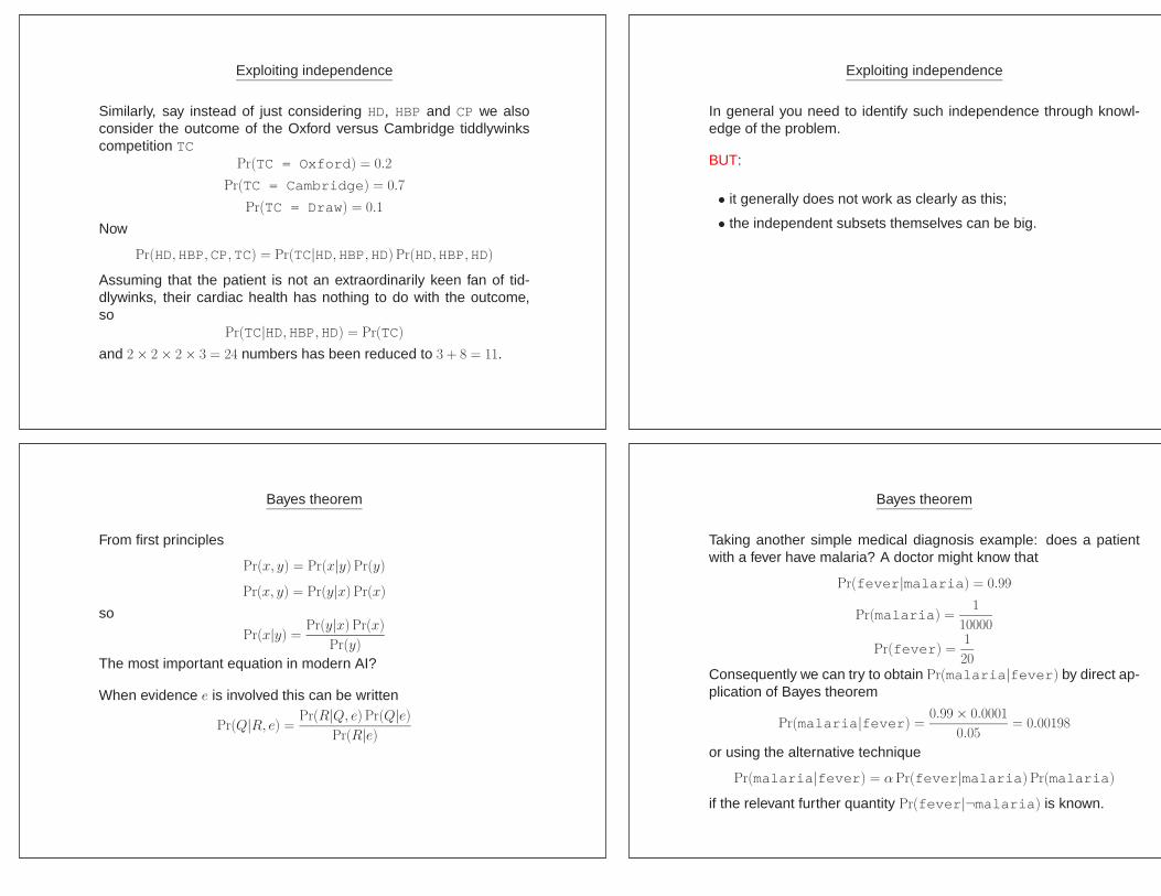
Exploiting independence
Similarly, say instead of just considering HD, HBP and CP we alsoconsider the outcome of the Oxford versus Cambridge tiddlywinkscompetition TC
Pr(TC = Oxford) = 0.2
Pr(TC = Cambridge) = 0.7
Pr(TC = Draw) = 0.1
Now
Pr(HD,HBP,CP,TC) = Pr(TC|HD,HBP,HD) Pr(HD,HBP,HD)
Assuming that the patient is not an extraordinarily keen fan of tid-dlywinks, their cardiac health has nothing to do with the outcome,so
Pr(TC|HD,HBP,HD) = Pr(TC)
and 2 × 2 × 2 × 3 = 24 numbers has been reduced to 3 + 8 = 11.
Exploiting independence
In general you need to identify such independence through knowl-edge of the problem.
BUT:
• it generally does not work as clearly as this;
• the independent subsets themselves can be big.
Bayes theorem
From first principles
Pr(x, y) = Pr(x|y) Pr(y)
Pr(x, y) = Pr(y|x) Pr(x)
so
Pr(x|y) =Pr(y|x) Pr(x)
Pr(y)
The most important equation in modern AI?
When evidence e is involved this can be written
Pr(Q|R, e) =Pr(R|Q, e) Pr(Q|e)
Pr(R|e)
Bayes theorem
Taking another simple medical diagnosis example: does a patientwith a fever have malaria? A doctor might know that
Pr(fever|malaria) = 0.99
Pr(malaria) =1
10000
Pr(fever) =1
20Consequently we can try to obtain Pr(malaria|fever) by direct ap-plication of Bayes theorem
Pr(malaria|fever) =0.99 × 0.0001
0.05= 0.00198
or using the alternative technique
Pr(malaria|fever) = α Pr(fever|malaria) Pr(malaria)
if the relevant further quantity Pr(fever|¬malaria) is known.

Bayes theorem
• Sometimes the first possibility is easier, sometimes not.
• Causal knowledge such as
Pr(fever|malaria)
might well be available when diagnostic knowledge such as
Pr(malaria|fever)
is not.
• Say the incidence of malaria, modelled by Pr(Malaria), sud-denly changes. Bayes theorem tells us what to do.
• The quantityPr(fever|malaria)
would not be affected by such a change.
Causal knowledge can be more robust.
Conditional independence
What happens if we have multiple pieces of evidence?
We have seen that to compute
Pr(HD|CP,HBP)
directly might well run into problems.
we could try using Bayes theorem to obtain
Pr(HD|CP,HBP) = α Pr(CP,HBP|HD) Pr(HD)
However while HD is probably manageable, a quantity such as Pr(CP,HBPmight well still be problematic especially in more realistic cases.
Conditional independence
However although in this case we might not be able to exploit inde-pendence directly we can say that
Pr(CP,HBP|HD) = Pr(CP|HD) Pr(HBP|HD)
which simplifies matters.
Conditional independence :
• Pr(A, B|C) = Pr(A|C) Pr(B|C)
• If we know that C is the case then A and B are independent.
Although CP and HBP are not independent, they do not directly influ-ence one another in a patient known to have heart disease.
This is much nicer!
Pr(HD|CP,HBP) = α Pr(CP|HD) Pr(HBP|HD) Pr(HD)
Naive Bayes
Conditional independence is often assumed even when it does nothold.
Naive Bayes :
Pr(A, B1, B2, . . . , Bn) = Pr(A)n∏
i=1
Pr(Bi|A)
Also known as Idiot’s Bayes .
Despite this, it is often surprisingly effective.

Uncertainty II - Bayesian Networks
Having seen that in principle, if not in practice, the full joint distribu-tion alone can be used to perform any inference of interest, we nowexamine a practical technique.
• We introduce the Bayesian network (BN) as a compact represen-tation of the full joint distribution.
• We examine the way in which a BN can be constructed.
• We examine the semantics of BNs.
• We look briefly at how inference can be performed.
Reading: Russell and Norvig, chapter 14.
Bayesian networks
Also called probabilistic/belief/causal networks or knowledge maps .
TW HD
CP HBP
• Each node is a random variable (RV).
• Each node Ni has a distribution
Pr(Ni|parents(Ni))
• A Bayesian network is a directed acyclic graph.
• Roughly speaking, an arrow from N to M means N directly af-fects M .
Bayesian networks
After a regrettable incident involving an inflatable gorilla, a famousCollege has decided to install an alarm for the detection of roofclimbers.
• The alarm is very good at detecting climbers.
• Unfortunately, it is also sometimes triggered when one of the ex-tremely fat geese that lives in the College lands on the roof.
• One porter’s lodge is near the alarm, and inhabited by a chap withexcellent hearing and a pathological hatred of roof climbers: healways reports an alarm. His hearing is so good that he some-times thinks he hears an alarm, even when there isn’t one.
• Another porter’s lodge is a good distance away and inhabited byan old chap with dodgy hearing who likes to watch his collectionof videos with the sound turned up.
Bayesian networks
Alarm
Climber
Lodge1 Lodge2
Goose
No: 0.95
Yes: 0.05
Pr(Climber)
Yes: 0.2
No: 0.8
Pr(Goose)
Pr(L1|A)
a 0.99
¬a 0.08 ¬a
a
Pr(L2|A)
0.6
0.001
Pr(A|C,G)
C G Pr(A|C,G)
Y 0.98NY
NY
YN
N
0.080.960.2
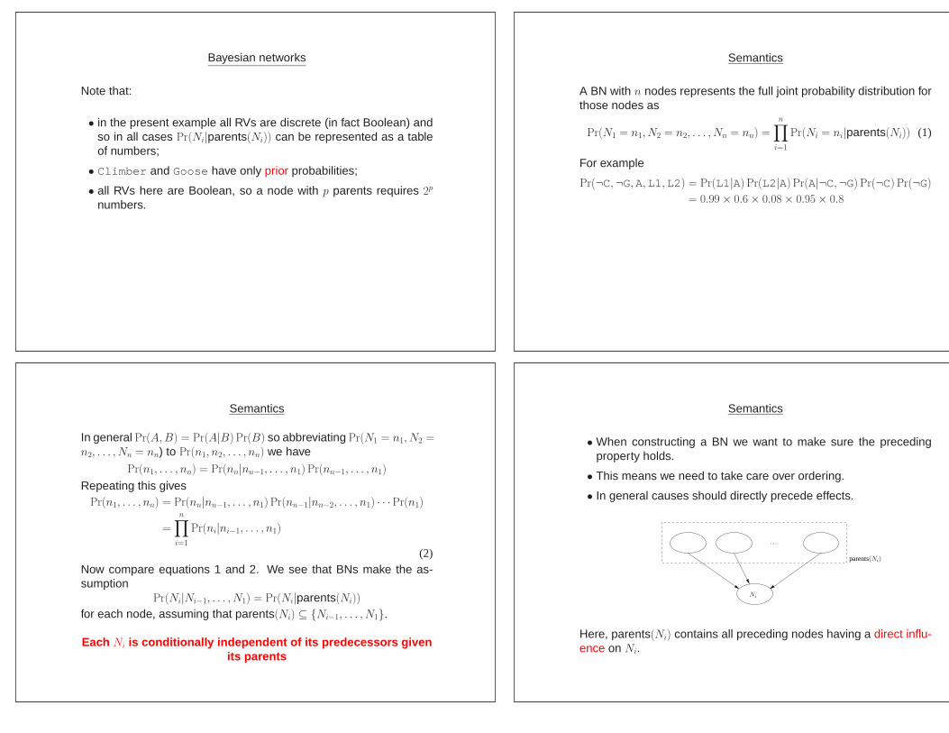
Bayesian networks
Note that:
• in the present example all RVs are discrete (in fact Boolean) andso in all cases Pr(Ni|parents(Ni)) can be represented as a tableof numbers;
• Climber and Goose have only prior probabilities;
• all RVs here are Boolean, so a node with p parents requires 2p
numbers.
Semantics
A BN with n nodes represents the full joint probability distribution forthose nodes as
Pr(N1 = n1, N2 = n2, . . . , Nn = nn) =
n∏
i=1
Pr(Ni = ni|parents(Ni)) (1)
For example
Pr(¬C,¬G,A,L1,L2) = Pr(L1|A) Pr(L2|A) Pr(A|¬C,¬G) Pr(¬C) Pr(¬G)
= 0.99 × 0.6 × 0.08 × 0.95 × 0.8
Semantics
In general Pr(A, B) = Pr(A|B) Pr(B) so abbreviating Pr(N1 = n1, N2 =n2, . . . , Nn = nn) to Pr(n1, n2, . . . , nn) we have
Pr(n1, . . . , nn) = Pr(nn|nn−1, . . . , n1) Pr(nn−1, . . . , n1)
Repeating this givesPr(n1, . . . , nn) = Pr(nn|nn−1, . . . , n1) Pr(nn−1|nn−2, . . . , n1) · · ·Pr(n1)
=n∏
i=1
Pr(ni|ni−1, . . . , n1)
(2)Now compare equations 1 and 2. We see that BNs make the as-sumption
Pr(Ni|Ni−1, . . . , N1) = Pr(Ni|parents(Ni))
for each node, assuming that parents(Ni) ⊆ {Ni−1, . . . , N1}.
Each Ni is conditionally independent of its predecessors givenits parents
Semantics
• When constructing a BN we want to make sure the precedingproperty holds.
• This means we need to take care over ordering.
• In general causes should directly precede effects.
· · ·
Ni
parents(Ni)
Here, parents(Ni) contains all preceding nodes having a direct influ-ence on Ni.

Semantics
Deviation from this rule can have major effects on the complexity ofthe network.
That’s bad! We want to keep the network simple:
• if each node has at most p parents and there are n Booleannodes, we need to specify at most n2p numbers...
• ...whereas the full joint distribution requires us to specify 2n num-bers.
So: there is a trade-off attached to the inclusion of tenuous althoughstrictly-speaking correct edges.
Semantics
As a rule, we should include the most basic causes first, then thethings they influence directly etc.
What happens if you get this wrong?
Example: add nodes in the order L2,L1,G,C,A.
Goose
Lodge1
Climber Alarm
Lodge2
Semantics
In this example:
• increased connectivity;
• many of the probabilities here will be quite unnatural and hard tospecify.
Once again: causal knowledge is preferred to diagnostic knowledge.
Semantics
As an alternative we can say directly what conditional independenceassumptions a graph should be interpreted as expressing. There aretwo common ways of doing this.
N1 A N2
P2P1
Any node A is conditionally independent of the Ni—its non-descendants—given the Pi—its parents.

Semantics
A M4
M1 M2 M3
M8
M5M6M7
Any node A is conditionally independent of all other nodes given theMarkov blanket Mi—that is, its parents, its children, and its children’sparents.
More complex nodes
How do we represent
Pr(Ni|parents(Ni))
when nodes can denote general discrete and/or continuous RVs?
• BNs containing both kinds of RV are called hybrid BNs.
• Naive discretisation of continuous RVs tends to result in both areduction in accuracy and large tables.
• O(2p) might still be large enough to be unwieldy.
• We can instead attempt to use standard and well-understood dis-tributions, such as the Gaussian.
• This will typically require only a small number of parameters to bespecified.
More complex nodes
Example: functional relationships are easy to deal with.
Ni = f(parents(Ni))
Pr(Ni = ni|parents(Ni)) =
{1 if ni = f(parents(Ni))0 otherwise
More complex nodes
Example: a continuous RV with one continuous and one discreteparent.
Pr(Speed of car|Throttle position,Tuned engine)
where SC and TP are continuous and TE is Boolean.
• For a specific setting of ET = true it might be the case that SCincreases with TP, but that some uncertainty is involved
Pr(SC|TP,et) = N(getTP + cet, σ2et)
• For an un-tuned engine we might have a similar relationship witha different behaviour
Pr(SC|TP,¬et) = N(g¬etTP + c¬et, σ2¬et)
There is a set of parameters {g, c, σ} for each possible value of thediscrete RV.

More complex nodes
Example: a discrete RV with a continuous parent
Pr(Go roofclimbing|Size of fine)
We could for example use the probit distribution
Pr(Go roofclimbing = true|size) = Φ
(t − size
s
)
where
Φ(x) =
∫ x
−∞
N(y)dy
and N(x) is the Gaussian distribution with zero mean and variance1.
More complex nodes
1
1
2
x
0
Φ(x)
1
1
2
size
t = 100
s controls slope
Pr(GRC = true|size)
More complex nodes
Alternatively, for this example we could use the logit distribution
Pr(Go roofclimbing = true|size) =1
1 + e(−2(t−size)/s)
which has a similar shape.
• Tails are longer for the logit distribution.
• The logit distribution tends to be easier to use...
• ...but the probit distribution is often more accurate.
Basic inference
We saw earlier that the full joint distribution can be used to performall inference tasks:
Pr(Q|e) =1
ZPr(Q ∧ e) =
1
Z
∑
u
Pr(Q, e, u)
where
• Q is the query variable
• e is the evidence
• u are the unobserved variables
• 1/Z normalises the distribution.

Basic inference
As the BN fully describes the full joint distribution
Pr(Q, u, e) =n∏
i=1
Pr(Ni|parents(Ni))
It can be used to perform inference in the obvious way.
Pr(Q|e) =1
Z
∑
u
n∏
i=1
Pr(Ni|parents(Ni))
• More sophisticated algorithms aim to achieve this more efficiently.
• For complex BNs we resort to approximation techniques.
Other approaches to uncertainty: Default reasoning
One criticism made of probability is that it is numerical whereas hu-man argument seems fundamentally different in nature:
• on the one hand this seems quite defensible. I certainly amnot aware of doing logical thought through direct manipulationof probabilities, but;
• on the other hand, neither am I aware of solving differential equa-tions in order to walk!
Default reasoning:
• does not maintain degrees of belief;
• allows something to be believed until a reason is found not to.
Other approaches to uncertainty: rule-based systems
Rule-based systems have some desirable properties:
• Locality: if we establish the evidence X and we have a rule X →Y then Y can be concluded regardless of any other rules.
• Detachment: once any Y has been established it can then beassumed. (It’s justification is irrelevant.)
• Truth-functionality: truth of a complex formula is a function of thetruth of its components.
These are not in general shared by probabilistic systems. What hap-pens if:
• we try to attach measures of belief to rules and propositions;
• we try to make a truth-functional system by, for example, makingbelief in X ∧ Y a function of beliefs in X and Y ?
Other approaches to uncertainty: rule-based systems
Problems that can arise:
1. Say I have the causal rule
Heart disease 0.95−→ Chest pain
and the diagnostic rule
Chest pain 0.7−→ Heart disease
Without taking very great care to keep track of the reasoning pro-cess, these can form a loop.
2. If in addition I have
Chest pain 0.6−→ Recent physical exertion
then it is quite possible to form the conclusion that with somedegree of certainty heart disease is explained by exertion, whichmay well be incorrect.

Other approaches to uncertainty: rule-based systems
In addition, we might argue that because heart disease is an expla-nation for chest pain the belief in physical exertion should decrease.
In general when such systems have been successful it has beenthrough very careful control in setting up the rules.
Other approaches to uncertainty: Dempster-Shafer theory
Dempster-Shafer theory attempts to distinguish between uncertaintyand ignorance.
Whereas the probabilistic approach looks at the probability of X, weinstead look at the probability that the available evidence supportsX.
This is denoted by the belief function Bel(X).
Example: given a coin but no information as to whether it is fair Ihave no reason to think one outcome should be preferred to another
Bel(outcome = head) = Bel(outcome = tail) = 0
Other approaches to uncertainty: Dempster-Shafer theory
These beliefs can be updated when new evidence is available. If anexpert tells us there is n percent certainty that it’s a fair coin then
Bel(outcome = head) = Bel(outcome = tail) =n
100×
1
2.
We may still have a “gap” in that
Bel(outcome = head) + Bel(outcome = tail) 6= 1.
Dempster-Shafer theory provides a coherent system for dealing withbelief functions.
Other approaches to uncertainty: Dempster-Shafer theory
Problems:
• the Bayesian approach deals more effectively with the quantifica-tion of how belief changes when new evidence is available;
• the Bayesian approach has a better connection to the concept ofutility, whereas the latter is not well-understood for use in con-junction with Dempster-Shafer theory.

Uncertainty III: exact inference in Bayesian networks
We now examine:
• the basic equation for inference in Bayesian networks, the latterbeing hard to achieve if approached in the obvious way;
• the way in which matters can be improved a little by a small mod-ification to the way in which the calculation is done;
• the way in which much better improvements might be possibleusing a still more informed approach, although not in all cases.
Reading: Russell and Norvig, chapter 14, section 14.4.
Performing exact inference
We know that in principle any query Q can be answered by the cal-culation
Pr(Q|e) =1
Z
∑
u
Pr(Q, e, u)
where Q denotes the query, e denotes the evidence, u denotes un-observed variables and 1/Z normalises the distribution.
The naive implementation of this approach yields the Enumerate-Joint-Ask algorithm, which unfortunately requires O(2n) time and spacefor n Boolean random variables (RVs).
Performing exact inference
In what follows we will make use of some abbreviations.
• C denotes Climber
• G denotes Goose
• A denotes Alarm
• L1 denotes Lodge1
• L2 denotes Lodge2
Instead of writing out Pr(C = ⊤), Pr(C = ⊥) etc we will write Pr(c),Pr(¬c) and so on.
Performing exact inference
Also, for a Bayesian network, Pr(Q, e, u) has a particular form ex-pressing conditional independences in the problem. For our earlierexample:
Alarm
Climber
Lodge1 Lodge2
Goose
No: 0.95
Yes: 0.05
Pr(Climber)
Pr(L1|A)
a 0.99
¬a 0.08
Yes: 0.2
No: 0.8
Pr(Goose)
¬a
a
Pr(L2|A)
0.6
0.001
Pr(A|C,G)
C G Pr(A|C,G)
Y 0.98NY
NY
YN
N
0.080.960.2
Pr(C, G,A, L1, L2) = Pr(C)Pr(G)Pr(A|C,G)Pr(L1|A)Pr(L2|A)

Performing exact inference
Consider the computation of the query Pr(C|l1, l2)
We have
Pr(C|l1, l2) =1
Z
∑
A
∑
G
Pr(C)Pr(G)Pr(A|C, G)Pr(l1|A)Pr(l2|A)
Here there are 5 multiplications for each set of values that appearsfor summation, and there are 4 such values.
In general this gives time complexity O(n2n) for n Boolean RVs.
Performing exact inference
Looking more closely we see that
Pr(C|l1, l2) =1
Z
∑
A
∑
G
Pr(C)Pr(G)Pr(A|C, G)Pr(l1|A)Pr(l2|A)
=1
ZPr(C)
∑
A
Pr(l1|A)Pr(l2|A)∑
G
Pr(G)Pr(A|C,G)
=1
ZPr(C)
∑
G
Pr(G)∑
A
Pr(A|C, G)Pr(l1|A)Pr(l2|A)
(3)
So for example...
Performing exact inference
So for example...
Pr(c|l1, l2) =1
ZPr(c)
(
Pr(g)
{Pr(a|c, g)Pr(l1|a)Pr(l2|a)
+Pr(¬a|c, g)Pr(l1|¬a)Pr(l2|¬a)
}
+Pr(¬g)
{Pr(a|c,¬g)Pr(l1|a)Pr(l2|a)
+Pr(¬a|c,¬g)Pr(l1|¬a)Pr(l2|¬a)
})
with a similar calculation for Pr(¬c|l1, l2).
Basically straightforward, BUT optimisations can be made.
Performing exact inference
Pr(l1|a)
Pr(l2|a)
Pr(l1|¬a)
Pr(l2|¬a)
Pr(a|c, g) Pr(¬a|c, g)
Pr(l1|a)
Pr(l2|a)
Pr(l1|¬a)
Pr(l2|¬a)
Pr(c)
Pr(g) Pr(¬g)
+
+
+
Pr(¬a|c,¬g)Pr(a|c,¬g)
Repeated Repeated

Optimisation 1: Enumeration-Ask
The enumeration-ask algorithm improves matters to O(2n) time andO(n) space by performing the computation depth-first.
However matters can be improved further by avoiding the duplicationof computations that clearly appears in the example tree.
Optimisation 2: variable elimination
Looking again at the fundamental equation (3)
1
ZPr(C)︸ ︷︷ ︸
C
∑
G
Pr(G)︸ ︷︷ ︸
G
∑
A
Pr(A|C,G)︸ ︷︷ ︸
A
Pr(l1|A)︸ ︷︷ ︸
L1
Pr(l2|A)︸ ︷︷ ︸
L2
where C,G,A, L1, L2 denote the relevant factors.
The basic idea is to evaluate (3) from right to left (or in terms of thetree, bottom up) storing results as we progress and re-using themwhen necessary.
Pr(l1|A) depends on the value of A. We store it as a table FL1(A).Similarly for Pr(l2|A).
FL1(A) =
(0.990.08
)
FL2(A) =
(0.6
0.001
)
as Pr(l1|a) = 0.99, Pr(l1|¬a) = 0.08 and so on.
Optimisation 2: variable elimination
Similarly for Pr(A|C,G), which is dependent on A, C and G
FA(A, C,G) =
A C G FA(A, C,G)⊤ ⊤ ⊤ 0.98⊤ ⊤ ⊥ 0.96⊤ ⊥ ⊤ 0.2⊤ ⊥ ⊥ 0.08⊥ ⊤ ⊤ 0.02⊥ ⊤ ⊥ 0.04⊥ ⊥ ⊤ 0.8⊥ ⊥ ⊥ 0.92
Can we writePr(A|C, G)Pr(l1|A)Pr(l2|A) (4)
asFA(A, C,G)FL1(A)FL2(A) (5)
in a reasonable way?
Optimisation 2: variable elimination
The answer is “yes” provided multiplication of factors is defined cor-rectly. Looking at (3)
1
ZPr(C)
∑
G
Pr(G)∑
A
Pr(A|C,G)Pr(l1|A)Pr(l2|A)
note that the values of the product (4) in the summation depend onthe values of C and G external to it, and the values of A themselves.So (5) should be a table collecting values for (4) where correspon-dences between RVs are maintained.
This leads to a definition for multiplication of factors best given byexample.

Optimisation 2: variable elimination
F(A, B)F(B,C) = F(A, B,C)
where
A B F(A, B) B C F(B,C) A B C F(A, B,C)⊤ ⊤ 0.3 ⊤ ⊤ 0.1 ⊤ ⊤ ⊤ 0.3 × 0.1⊤ ⊥ 0.9 ⊤ ⊥ 0.8 ⊤ ⊤ ⊥ 0.3 × 0.8⊥ ⊤ 0.4 ⊥ ⊤ 0.8 ⊤ ⊥ ⊤ 0.9 × 0.8⊥ ⊥ 0.1 ⊥ ⊥ 0.3 ⊤ ⊥ ⊥ 0.9 × 0.3
⊥ ⊤ ⊤ 0.4 × 0.1⊥ ⊤ ⊥ 0.4 × 0.8⊥ ⊥ ⊤ 0.1 × 0.8⊥ ⊥ ⊥ 0.1 × 0.3
Optimisation 2: variable elimination
This process gives us
FA(A, C,G)FL1(A)FL2(A) =
A C G⊤ ⊤ ⊤ 0.98 × 0.99 × 0.6⊤ ⊤ ⊥ 0.96 × 0.99 × 0.6⊤ ⊥ ⊤ 0.2 × 0.99 × 0.6⊤ ⊥ ⊥ 0.08 × 0.99 × 0.6⊥ ⊤ ⊤ 0.02 × 0.08 × 0.001⊥ ⊤ ⊥ 0.04 × 0.08 × 0.001⊥ ⊥ ⊤ 0.8 × 0.08 × 0.001⊥ ⊥ ⊥ 0.92 × 0.08 × 0.001
Optimisation 2: variable elimination
How about
FA,L1,L2(C,G) =∑
A
FA(A, C,G)FL1(A)FL2(A)
To denote the fact that A has been summed out we place a bar overit in the notation.
∑
A
FA(A, C,G)FL1(A)FL2(A) =FA(a,C,G)FL1(a)FL2(a)
+ FA(¬a,C,G)FL1(¬a)FL2(¬a)
where
FA(a,C,G) =
C G⊤ ⊤ 0.98⊤ ⊥ 0.96⊥ ⊤ 0.2⊥ ⊥ 0.08
FL1(a) = 0.99 FL2(a) = 0.6
and similarly for FA(¬a,C,G), FL1(¬a) and FL2(¬a).
Optimisation 2: variable elimination
FA(a,C,G)FL1(a)FL2(a) =
C G⊤ ⊤ 0.98 × 0.99 × 0.6⊤ ⊥ 0.96 × 0.99 × 0.6⊥ ⊤ 0.2 × 0.99 × 0.6⊥ ⊥ 0.08 × 0.99 × 0.6
FA(¬a,C,G)FL1(¬a)FL2(¬a) =
C G⊤ ⊤ 0.02 × 0.08 × 0.001⊤ ⊥ 0.04 × 0.08 × 0.001⊥ ⊤ 0.8 × 0.08 × 0.001⊥ ⊥ 0.92 × 0.08 × 0.001
FA,L1,L2(C,G) =
C G⊤ ⊤ (0.98 × 0.99 × 0.6) + (0.02 × 0.08 × 0.001)⊤ ⊥ (0.96 × 0.99 × 0.6) + (0.04 × 0.08 × 0.001)⊥ ⊤ (0.2 × 0.99 × 0.6) + (0.8 × 0.08 × 0.001)⊥ ⊥ (0.08 × 0.99 × 0.6) + (0.92 × 0.08 × 0.001)

Optimisation 2: variable elimination
Now, say for example we have ¬c, g. Then doing the calculationexplicitly would give∑
A
Pr(A|¬c, g)Pr(l1|A))Pr(l2|A)
= Pr(a|¬c, g)Pr(l1|a)Pr(l2|a) + Pr(¬a|¬c, g)Pr(l1|¬a)Pr(l2|¬a)
= (0.2 × 0.99 × 0.6) + (0.8 × 0.08 × 0.001)
which matches!
Continuing in this manner form
FG,A,L1,L2(C,G) = FG(G)FA,L1,L2(C,G)
sum out G to obtain FG,A,L1,L2(C) =∑
G FG(G)FA,L1,L2(C,G), form
FC,G,A,L1,L2 = FC(C)FG,A,L1,L2(C)
and normalise.
Optimisation 2: variable elimination
What’s the computational complexity now?
• for Bayesian networks with suitable structure we can perform in-ference in linear time and space;
• however in the worst case it is #P -hard, which is worse than NP -hard.
Consequently, we may need to resort to approximate inference.
Exercises
Exercise 1: This question revisits the Wumpus World, but now ourhero (let’s call him Wizzo the Incompetent), having learned someprobability by attending Artificial Intelligence II , will use probabilis-tic reasoning instead of situation calculus.
Wizzo, through careful consideration of the available knowledge onWumpus caves, has established that each square contains a pit withprior probability 0.3, and pits are independent of one-another. LetPiti,j be a Boolean random variable (RV) denoting the presence ofa pit at row i, column j. So for all i, j
Pr(Piti,j = ⊤) = 0.3 (6)Pr(Piti,j = ⊥) = 0.7 (7)
In addition, after some careful exploration of the current cave, ourhero has discovered the following.
Exercises
1
2
3
4
1 2 3 4
B
OKOK OK
OK
B?
Pit1,1 = ⊥
Pit1,2 = ⊥
Pit1,3 = ⊥
Pit2,3 = ⊥
B denotes squares where a breeze is perceived. Let Breezei,j be aBoolean RV denoting the presence of a breeze at i, j
Breeze1,2 = Breeze2,3 = ⊤ (8)Breeze1,1 = Breeze1,3 = ⊥ (9)
Wizzo is considering whether to explore the square at 2, 4. He will doso if the probability that it contains a pit is less than 0.4. Should he?

Exercises
Hint : The RVs involved are Breeze1,2,Breeze2,3,Breeze1,1,Breeze1,3
and Piti,j for all the i, j. You need to calculate
Pr(Pit2,4|all the evidence you have so far)
Exercises
Exercise 2: Continuing with the running example of the roof-climberalarm...
The porter in lodge 1 has left and been replaced by a somewhatmore relaxed sort of chap, who doesn’t really care about roof-climbersand therefore acts according to the probabilities
Pr(l1|a) = 0.3 Pr(¬l1|a) = 0.7Pr(l1|¬a) = 0.001 Pr(¬l1|¬a) = 0.999
Your intrepid roof-climbing buddy is on the roof. What is the probabil-ity that lodge 1 will report him? Use the variable elimination algorithmto obtain the relevant probability. Do you learn anything interestingabout the variable L2 in the process?
Exercises
Exercise 3: Exam question, 2006, paper 8, question 9.
87


