
Types of DataHow to Calculate Distance?
Dr. Ryan Benton
January 29, 2009

Book Information
Data Mining, Concepts and Techniques Chapter 7, Section 2, Types of Data in Cluster
AnalysisAdvances in Instance-Based Learning Algorithms, Dissertation by D. Randall Wilson, August 1997. Chapters 4 and 5.
Prototype Styles of Generalization Thesis by D. Randall Wilson, August 1994. Chapters 3.

Data
Each instance (point, record, example)Composed of one or more features.
FeatureComposed of a data typeData type has a range of values.

Data Types
Interval-ScaledReal IntegerComplex
Ratio-ScaledBinarySymmetricAsymmetric

Data Types
CategoricalOrdinalDiscreteContinuous
OthersVectorsShapeEtc.

Comparing Instances
How does one compare instances?ClusteringClassification
Instance-Base ClassifiersArtificial Neural NetworksSupport Vector Machines
Distance Functions (Measures)

Distance Measures
Propertiesd(i,j) 0d(i,i) = 0d(i,j) = d(j,i)d(i,j) d(i,k) + d(k,j)

Interval-Scaled Variables
Many Different Distance MeasuresEuclideanManhattan (City Block)Minkowski
For purpose of discussion, assume all features in data point are Interval-Scaled.

Euclidean
Also called the L2 normAssumes a straight-line from two points
Where i, j are two different instancesn is the number of interval-featuresXiz is the value at zth feature value for i.
22
22
2
11...),(
jninjijixxxxxxjid

Manhattan
Also classed the L1 normNon-Linear.
Where i, j are two different instancesn is the number of interval-featuresXiz is the value at zth feature value for i.
jninjijixxxxxxjid ...),(
2211

Minkowski
Euclidean and ManhattanSpecial Cases
Where p is a positive integer
Also called the Lp norm fuction
pp
jnin
p
ji
p
ji xxxxxxjid1
2211 ...),(

Minkowski
Not all features are equal.Some are irrelevantSome are should be highly influential
Where, Wz is the ‘weight’ Wz >= 0.
pp
jninn
p
ji
p
ji xxwxxwxxwjid1
222111 ...),(

Example
x1 = (1,2), x2 = (3,5)
Euclidean:
Manhattan:
Minkowski (q=3):
61.35231),( 22 jid
3.272785231),( 313
133 jid
55231),( jid

Other Distance Measures
Camberra
Chebychev
Quadratic
Mahalanobis
Correlation
Chi-Squared
Kendall’s Rank Correlation
And so forth.
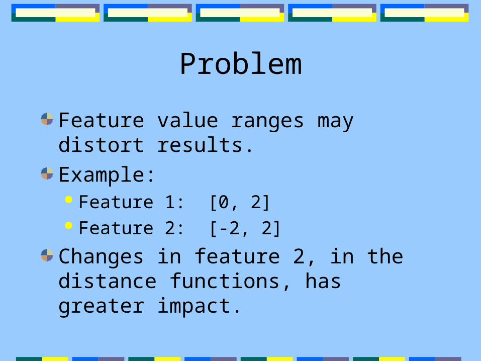
Problem
Feature value ranges may distort results.
Example:Feature 1: [0, 2]Feature 2: [-2, 2]
Changes in feature 2, in the distance functions, has greater impact.

Scaling
Scale each feature to a range [0,1] [-1, 1]
Possible IssueSay feature range is [0, 2].99% of the data >= 1.5
Outliers have large impact on distanceNormal values have almost none.

Normalize
Modify each feature soMean (mf) = 0Standard Deviation (f) = 1
,
where yif is the new feature valueN is the number of data points.
f
fifif
mxy
22
2
2
1 ...1
fNffffff mxmxmxN
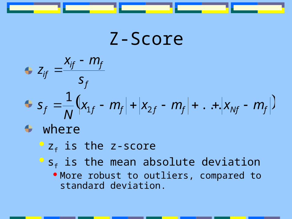
Z-Score
where zf is the z-scoresf is the mean absolute deviation
More robust to outliers, compared to standard deviation.
f
fifif s
mxz
fNffffff mxmxmxN
s ...1
21
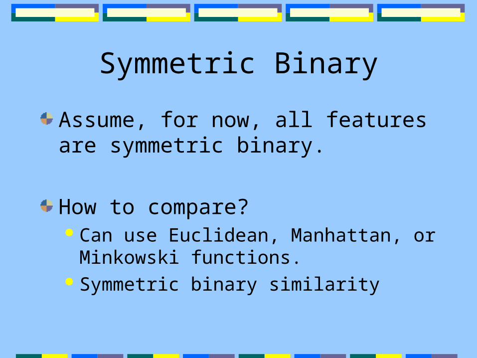
Symmetric Binary
Assume, for now, all features are symmetric binary.
How to compare?Can use Euclidean, Manhattan, or
Minkowski functions.Symmetric binary similarity

Symmetric Binary
q, r, s and t are counts.
Object i
Object j
1
0
sum
sum1 0
t
r
r + t
s + t
q + r
p
s
q
q + s

Symmetric Binary
PropertiesRange is [0, 1]0 indicates perfect match1 indicates no matches
psr
jid),(

Asymmetric Binary
Assume, for now, all features are asymmetric binary.
Like Symmetric BinaryCan use Euclidean, Manhattan, or
Minkowski functions.
Alternately, can useAsymmetric binary similarity

Asymmetric Binary
q, r, s and t are counts.
Object i
Object j
1
0
sum
sum1 0
t
r
r + t
s + t
q + r
p
s
q
q + s
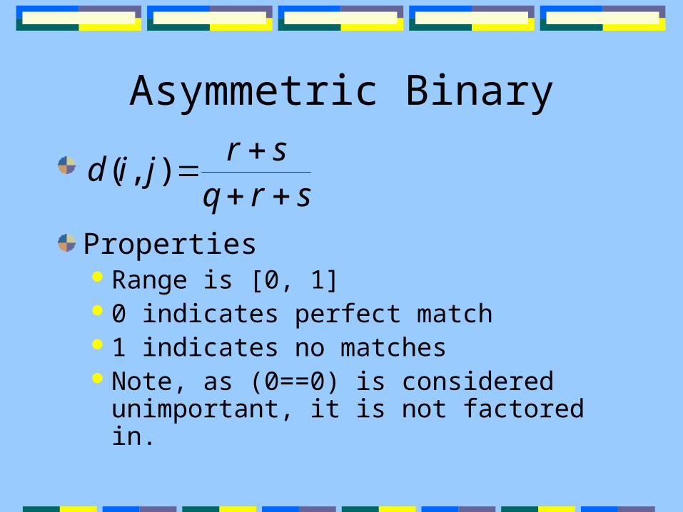
Asymmetric Binary
PropertiesRange is [0, 1]0 indicates perfect match1 indicates no matchesNote, as (0==0) is considered unimportant,
it is not factored in.
srqsr
jid
),(
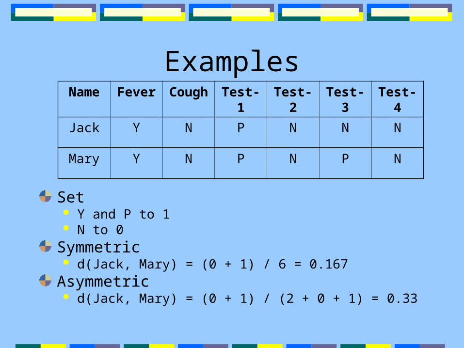
Examples
Set Y and P to 1 N to 0
Symmetric d(Jack, Mary) = (0 + 1) / 6 = 0.167
Asymmetric d(Jack, Mary) = (0 + 1) / (2 + 0 + 1) = 0.33
Name Fever Cough Test-1 Test-2 Test-3 Test-4
Jack Y N P N N N
Mary Y N P N P N

Categorical
Wherep = number of variablem = number of matches
pmp
jid),(

Example
d(2, 1) = (1 – 0) / 1 = 0
d(1, 4) = (1 – 1) / 1 = 1
Student Test-1
(categorical)
Test-2
(ordinal)
Test-3
(ratio)
1 Code-A Excellent 445
2 Code-B Fair 22
3 Code-C Good 164
4 Code-A Excellent 1,210

Categorical
WeightingCan add weights to
Increase effect of m Increase importance of variables with more
states Can do this for Binary as well.
ConventionSome of weights should be equal to 1.

Categorical – Other measures
Value Difference Metric For Classification problems (not Clustering). Estimates conditional probabilities for each feature
value for each class. Distance base on difference in conditional
probabilities. Includes a weighting scheme.
Modified Value Difference Metric Handles weight estimation differently.

Value Difference Metric (VDM)
Where P(xif,g) = conditional probability of the class g
occuring, given the value xi for feature f. C is the number of classes n is the number of features q is either 1 or 2.
Note, for simplification, weights are not included.
qn
f
C
gjfif gxPgxPjid
1 1),(),(),(

Ordinal
Assume all Features are Ordinal.Feature f has Mf ordered states, representing ranking 1, 2, …, Mf.For each instance i For each feature f
Replace value xif by corresponding rank rif
To calculate d(i,j) Use Interval-Scaled Distance Functions.
],...,1[ fif Mr

Ordinal
Like Interval-ScaledDifferent Ordinal features may have
different number of states.This leads to different features having
different implicit weights.Hence, scaling necessary.
1
1
f
ifif M
ry

Example
Mappings Fair = 1, Good = 2, Excellent = 3
Normalized Values Fair = 0.0, Good = 0.5, Excellent = 1.0
Student Test-1
(categorical)
Test-2
(ordinal)
Test-3
(ratio)
1 Code-A Excellent 445
2 Code-B Fair 22
3 Code-C Good 164
4 Code-A Excellent 1,210

Example
Euclidean:
Student Test-1
(categorical)
Test-2
(ordinal)
Test-3
(ratio)
1 Code-A Excellent 445
2 Code-B Fair 22
3 Code-C Good 164
4 Code-A Excellent 1,210
5.05.00)3,2( 2 d
Ordinal – Other Measures
Hamming Distance
Absolute Difference
Normalized Absolute Difference
Normalized Hamming Distance

Ratio-Scaled
Can’t treat directly as Interval-ScaledThe scale for Ratio-Scaled would lead to
distortion of results.
Apply a logarithmic transformation first.
yif = log(xif)Other type of transformation.
Treat result as continuous Ordinal Data.

Example
Student Test-1
(categorical)
Test-2
(ordinal)
Test-3
(ratio)
Test-3
(logarithmic)
1 Code-A Excellent 445 2.68
2 Code-B Fair 22 1.34
3 Code-C Good 164 2.21
4 Code-A Excellent 1,210 3.08
Euclidean: 87.021.208.3)3,4( 2 d

Mixed Types
The above approaches assumed that all features are the same type!
This is rarely the case.
Need a distance function that handles all types.

Mixed Distance
Whereij, for feature f is
0 If either xif or xjf is missing
(xif == xjf == 0) and f is asymmetric binary
Else 1
p
f
fij
p
f
fij
fij d
jid
1
1),(

Mixed Distance
Where If feature f is
Interval-scaled, use this formula
Where h runs over non-missing values for feature f.
Ensures distance returned is in range [0,1].
hfhhfh
jfiffij xx
xxd
minmax

Mixed Distance
Where If feature f is
Binary or categorical If xif == xjf, dij = 0
Else, dij = 1
Ordinal Compute ranks and apply the ordinal scaling Then use the interval-scaled distance measure.

Mixed Distance
Where If feature f is
Ratio-Scaled Do logarithmic (or similar) transform and then apply
interval-scaled distance. Or, treat as ordinal data.

Mixed Distance
Distance calculation for each feature will be 0 to 1.
Final distance calculation will be [0.0, 1.0]
p
f
fij
p
f
fij
fij d
jid
1
1),(

Example
Student Test-1
(categorical)
Test-2
(ordinal)
Test-3
(ratio)
Test-3
(logarithmic)
1 Code-A Excellent 445 2.68
2 Code-B Fair 22 1.34
3 Code-C Good 164 2.21
4 Code-A Excellent 1,210 3.08
92.03
34.108.3|68.234.1|
01|10|
1)1(1)1,2(
d
Mixed Distance
ProblemsDoesn’t permit use, for interval-scaled,
more advanced distance functions.Binary and categorical values have more
potential impact than other types of features.
Mixed Distance
MinkowskiHeterogeneous Overlap-Euclidean MetricHeterogeneous Value Difference MetricInterpolated Value Difference MetricWindowed Value Difference MetricK* Violates some of the conditions for distance
measure.
Not a complete list.

Questions?


