
TUITION ELASTICITY AT THE COLLEGE LEVEL AND ITS EFFECT ON
DIFFERENTIAL TUITION RATES
A Dissertation
by
MAX DUERY MENZIES III
Submitted to the Office of Graduate and Professional Studies of
Texas A&M University
in partial fulfillment of the requirements for the degree of
DOCTOR OF PHILOSOPHY
Chair of Committee, Glenda Musoba
Committee Members, David Bessler
Vicente Lechuga
Yvonna Lincoln
Head of Department, Mario Torres, Jr.
December 2017
Major Subject: Educational Administration
Copyright 2017 Max D. Menzies III

ii
ABSTRACT
Increasing higher education enrollment and decreasing state and national funding has
created a fiscal problem for higher education institutions in the United States. Differential tuition
charged to a variety of subsets of students is increasingly used to close funding gaps. This
research uses demand analysis and elasticities to determine differences between eight colleges at
a public university to determine which, if any, should be charging differential tuition. Impacts of
potential changes to tuition rates on student access are discussed.
Demand equations were created using ordinary least squares for eight colleges,
Agriculture, Architecture, Business, Education, Engineering, Geosciences, Liberal Arts, and
Sciences, using college applications as the dependent variable and assorted cost and
macroeconomic variables as independent variables. A second model was determined using
Directed Acyclic Graph theory and used to create a model for to answer policy questions.
Own-price elasticities (OPE) calculated from the colleges with significant variables in the
policy models ranged from .3 to -1.64. Two colleges showed as elastic, OPE with an absolute
value of greater than 1, indicating that a decrease in tuition would increase revenue and
enrollments. One college was inelastic, OPE with an absolute value of less than 1, indicating that
while an increase in tuition would lower enrollment, it would increase revenue. Engineering had
a calculated OPE that was positive, indicating the possibility that demand changed at a faster rate
than supply. Charging the correct form of differential tuition at a 10% level change to these
colleges could result in over $4 million additional revenue from first-year students alone.
It is suggested to consider differential tuition plan based on calculated elasticities to
generate more revenue. If implemented, a large percentage of the funds should be used to create

iii
institution-level, need-based, financial aid for students from low socioeconomic and minority
backgrounds. The aid should be in the form of grants to reduce the risk of students graduating
with high student debt.

iv
DEDICATION
This work is dedicated to my family, my mother and father, LaWanda and Duery
Menzies, my sister and brother-in-law, Misti and Decky Spiller, my nieces, Menzi and Chastain
Spiller, and my nearly countless aunts, uncles, and cousins.
I want to especially dedicate this to my dad and mom. Dad, you have been the constant
guiding light for me personally and for our entire family. You have been the solid foundation for
all our lives and the way you have lived your life fills me with pride and a desire to be just like
you. Love you Pop!
Mom, your constant "encouragement" is the only reason I was ever able to finish this!
Even a full time job was not a good excuse for you! I dearly wish you could be there the day I
finally become a doctor. I am sorry it took me so long and you have to miss it. I hope you are
watching me walk across the stage from up there in heaven. And I hope you are proud of me. I
know you will be in my thoughts on that day. I love you so much!
v
ACKNOWLEDGEMENTS
I would like to thank my committee chair, Dr. Musoba, and my committee members, Dr.
Bessler, Dr. Lechuga, and Dr. Lincoln for their support and guidance during my research and
writing.
Dr. Musoba, thank you so much for your help. I know it took a long time, but I could not
have done it without your mentoring. You were truly an asset and I am very grateful.
Thank you Dr. Bessler for being a wonderful mentor and colleague for the past ten years.
Specifically, thanks for the refresher on Directed Graphs and the software that made this analysis
possible.
Thank you Dr. Lechuga for your help during this research and for your wisdom in class. I
still remember the Higher Education class I took with you. Yes, it was late at night and there
were a lot of opinions in the room. But we all learned a lot about the real issues in higher
education.
Dr. Lincoln, I want to especially thank you for being my temporary chair before Dr.
Musoba arrived at Texas A&M. You helped me through prelims and were a blessing. I
thoroughly enjoyed your course on the History of Higher Education. I learned more in that class
than in any other history class I have ever taken! And your proposal class was the foundation of
this research. Without that late night course I would never have started this project, much less
finished!

vi
Thanks also go to the staff of the Department of Education, particularly Joyce Nelson.
Joyce helped me over all these long years with a mountain of paperwork and deadlines. Thanks
so much!
I want to thank my friends for their support throughout the years. I know I caused us to
miss out on lots of concerts and football games because I was "working on my paper", but your
support did mean the world to me.
I want to thank my friends and colleagues in the Department of Agricultural Economics.
It has been a long journey and I could not have done it without your friendship and care.
I would like to thank my whole family. I have so many extended family members that to
list all of you would push me over the page limit! You are all so important to me and I thank you
for your encouragement and love.
Thanks to my sister and brother-in-law for being my main sounding boards and putting
up with my not helping with our cattle as much as I should. Love you both and miss you!
Thanks to my nieces for being my main distractions! You girls are the best! At being the
butt of my jokes! Kidding! Kinda.... Love you!
Finally, I want to thank my mom and dad. Your love and strength have been my pillars. I
am a better person because I have your examples in my life. If I lead a live that is in your
footsteps and by your morals, I will have accomplished all that a man can accomplish. Love you
so much!

vii
CONTRIBUTORS AND FUNDING SOURCES
Contributors
This work was supervised by a dissertation committee consisting of Professor Glenda
Musoba, Professor Vicente Luchuga, and Professor Yvonna Lincoln of the Deparement of
Education Administration and Human Resource Developmentand Professor David Bessler of the
Department of Agricultural Economics.
Statistical support for work in Chapter Four was provided by Dr. David Bessler. All other
work for the dissertation was completed independently by the student.
Funding Sources
There are no outside funding contributions to acknowledge related to the research and
compilation of this document.

viii
TABLE OF CONTENTS
Page
ABSTRACT ........................................................................................................................... ii
DEDICATION ....................................................................................................................... iv
ACKNOWLEDGEMENTS ................................................................................................... v
CONTRIBUTORS AND FUNDING SOURCES ................................................................. vii
TABLE OF CONTENTS ...................................................................................................... viii
LIST OF FIGURES ............................................................................................................... x
LIST OF TABLES ................................................................................................................. xi
CHAPTER I STATEMENT OF THE PROBLEM ............................................................... 1
Problem Statement ..................................................................................................... 1
Theoretical Framework .............................................................................................. 4
Research Objectives ................................................................................................... 8
Research Hypotheses ................................................................................................ 9
Definitions ................................................................................................................. 12
CHAPTER II LITERATURE REVIEW ............................................................................... 18
Human Capital Theory ............................................................................................... 18
Enrollment Demand Elasticity ................................................................................... 21
Differential Tuition .................................................................................................... 41
CHAPTER III METHODOLOGY ........................................................................................ 47
Research Questions .................................................................................................... 47
Research Design......................................................................................................... 49
Summary .................................................................................................................... 66
CHAPTER IV RESULTS ...................................................................................................... 68
Complete Forecast Model .......................................................................................... 68
Policy Model .............................................................................................................. 87

ix
CHAPTER V IMPLICATIONS AND CONCLUSIONS...................................................... 113
Summary ................................................................................................................... 113
Conclusions ............................................................................................................... 122
Limitations ................................................................................................................ 129
Recommendations for Future Research .................................................................... 130
REFERENCES ...................................................................................................................... 131
APPENDIX A ........................................................................................................................ 139
APPENDIX B ........................................................................................................................ 144
APPENDIX C ........................................................................................................................ 148

x
LIST OF FIGURES
FIGURE Page
1 Typical Demand Curve ........................................................................................ 4
2 Market-clearing or Equilibrium Point .................................................................. 6
3 Applications in Eight Colleges at State U from 2003-2015 ................................ 51
4 State U Tuition for Eight Colleges During Years 2002-2015.............................. 53
5 State U University-wide Fees .............................................................................. 54
6 Four-year and Two-year Competitor Tuition Rates for 2003-2015 ..................... 55
7 Texas PCDI for 2003-2015 .................................................................................. 56
8 Texas Unemployment Rate and Stafford Loan Rate ........................................... 57
9 College Graduates Wages as a Percentage of High School Graduates Wages .... 59

xi
LIST OF TABLES
TABLE Page
1 Dickey-Fuller Test Statistics ................................................................................ 61
2 Expected Signs of Independent Variables ........................................................... 63
3 R-squared for Linear and Log-Log Models for Eight Colleges ........................... 69
4 P-values for Eight Colleges Using Linear Complete Model ............................... 71
5 P-values for Eight Colleges Using Log-Log Complete Model ............................ 73
6 Regression Results for the College of Agriculture and Life Sciences Complete
Model ................................................................................................................... 75
7 Regression Results for the College of Architecture Complete Model ................. 77
8 Regression Results for the College of Business Complete Model ...................... 79
9 Regression Results for the College of Education Complete Model .................... 81
10 Regression Results for the College of Engineering Complete Model ................. 82
11 Regression Results for the College of Geosciences Complete Model ................. 84
12 Regression Results for the College of Liberal Arts Complete Model ................. 85
13 Regression Results for the College of Sciences Complete Model ....................... 86
14 TETRAD II Results for Eight Colleges ............................................................... 88
15 R-squared Results for Policy Model .................................................................... 89
16 Adjusted R-squared Values for Complete and Policy Models ............................ 90
17 P-values for Linear Policy Model ........................................................................ 91
18 P-values for Log-log Policy Model ...................................................................... 91
19 Regression Results for College of Agriculture Policy Model ............................. 92
20 Log-log Form Elasticities for College of Agriculture Models............................. 93
21 Elasticities for College of Agriculture Linear Complete Model .......................... 95
xii
TABLE Page
22 Elasticities for College of Agriculture Linear Policy Model ............................... 96
23 Regression Results for College of Architecture Policy Model ............................ 97
24 Log-log Form Elasticities for College of Architecture Models ........................... 98
25 Elasticities for College of Architecture Linear Complete Model ........................ 99
26 Regression Results for College of Business Policy Model .................................. 100
27 Elasticities for College of Business Linear Policy Model ................................... 101
28 Regression Results for College of Education Policy Model ................................ 102
29 Elasticities for College of Education Linear Policy Model ................................. 103
30 Regression Results for College of Engineering Policy Model ............................ 104
31 Elasticities for College of Engineering Linear Policy Model .............................. 105
32 Regression Results for College of Geosciences Policy Model ............................ 106
33 Log-log Form Elasticities for College of Geosciences Models ........................... 106
34 Elasticities for College of Geosciences Linear Policy Model ............................. 107
35 Regression Results for College of Liberal Arts Policy Model ............................ 108
36 Elasticities for College of Liberal Arts Linear Policy Model .............................. 109
37 Regression Results for College of Sciences Policy Model .................................. 110
38 Elasticities for College of Sciences Linear Policy Model ................................... 111
39 Revenue Changes for 5 and 10% Tuition Changes Per Semester ....................... 118
40 Total Revenue Effects for State U for 5 and 10% Tuition Changes Per
Semester, All Colleges ......................................................................................... 120
41 Total Revenue Effects for State U for 5 and 10% Tuition Changes Per
Semester, Only Significant Colleges ................................................................... 121

1
CHAPTER I
STATEMENT OF THE PROBLEM
This chapter provides a description of the problem associated with increasing student
tuition at universities around the United States that has been magnified by the combination of
decreasing state appropriations and rising costs. The theoretical framework the study is based on
is presented as well as the relevant research questions and hypotheses. Key terms and definitions
are provided at the end of the chapter.
Problem Statement
Higher education in the United States has reached a critical mass. Population numbers
continue to rise taking student enrollment demand with them. Since 1980, enrollment in higher
education has increased in all areas and is now approaching 18 million undergraduate and 3
million graduate students (U.S. Department of Education, 2013). State and federal funding has
risen in response, but has not kept pace with growth or inflation. The gap between expenditures
and public funding has widened, causing increases in tuition and fees in many states. A parallel
problem resulting from the funding gap is a reduction in the quality of education, student success
rates, and student access. Barring a paradigm shift in how higher education is viewed in
America, the only solutions to the funding shortfalls appear to be massive increases in public
support or in student tuition.
The problem with either alternative is that the American public increasingly sees higher
education institutions as caring more about their bottom line and less about the student. A 2010
survey from the National Center for Public Policy and Higher Education found that people were
concerned with some of the ways colleges were mimicking the business world. The subjects of

2
the survey related their frustration with higher education and their belief that universities could
be cost-effective and allow greater access without substantial increases in funding. In fact, nearly
65% of the respondents believe that college costs are rising faster than other costs including
food, energy, and health care (Immerwahr, Johnson, Ott, & Rochkind, 2010). Tuition has
increased at a rapid pace the past three decades. Since the scholastic year 1980-81, tuition and
fees have increased in inflation-adjusted prices from 2.3% to 4.1% per year for private schools,
3.7% to 4.3% per year for four-year public schools, and 1.9% to 5.0% for public two-year
schools. Public four-year tuition prices are 331% higher than comparable prices in 1983 even
after factoring in inflation (College Board, 2013).
In addition to concerns about higher tuition, recent economic downturns have shown that
increased public funding, be it state or federal, will not be forthcoming. The intervals it takes for
state higher education funding once reduced to return to pre-cut levels have been increasing the
past few decades. In the 1980s, 76% of the states that cut funding restored the cuts within five
years. In the 1990s, that number had fallen to 58%. Recent trends are more serious. In the 2000s,
fewer than 40% of states that have cut higher education have recovered in five years (Ciciora,
2010). Most experts believe it will take at least ten years for many states to recover from the
current round of cuts. This has dramatic repercussions for all parties involved. Paul Lingenfelter,
President of the State Higher Education Executive Officers, commented, “No country has ever
increased the quality and size of its higher education system by consistently decreasing its budget
for education” (Lingenfelter, 2009, p. 1). The reality of the current situation in America is one of
public demands for both increasing enrollment and increasing quality of education. Increasing
tuition may be the only possible answer. However, differential tuition rates, charging different

3
types of individuals differing tuitions for the same education, could prove an interesting counter
solution.
Differential tuition is a difficult political issue. Is it fair to charge different people
different rates for the same education? Differential tuition is accepted for areas such as graduate
school, professional school, and more recently, distance education. Is there justification,
however, for charging an Engineering major higher tuition than an English major? One of these
certainly can expect higher salaries than the other upon graduation, but the possibility of pricing
low-income students out of certain majors raises concerns. Additionally, one of the goals of the
United States is to increase interest in the disciplines of science, technology, engineering, and
mathematics (STEM) among all students. Would making those educations cost more limit ability
of those disciplines to grow?
Tuition increases across the board may not be economically viable or even wise. Several
summaries of enrollment demand studies find that students are relatively unresponsive to
changes in tuition price (Heller, 1997; Leslie & Brinkman, 1987). However these studies have
been mostly focused on education in general. Looking at individual colleges or departments may
show different results. One measure of responsiveness in economic theory is elasticity or how
much one variable changes in response to changes in another variable. Variables can be inelastic,
not responsive, or elastic, responsive. Economic theory may be used to classify a department or
college's enrollment demands as inelastic or elastic and provide recommendations for differential
tuition rates that would maximize revenues for either case. Goods with inelastic demands can
increase revenue with higher prices, while elastic demands increase revenue with lower prices.
Thus high demand departments would cost more causing enrollment to decrease slightly, while
increasing revenue. Conversely, low demand departments would cost less increasing enrollment

4
and revenue at the same time. From a pure economic standpoint, utilizing differential tuition to
charge different amounts to different students according to these elasticities could increase
revenue beyond that received from simple straight-line tuition.
Theoretical Framework
One of the fundamental building blocks of economic analysis is the concept of demand
(Henderson, 2008). The school of economic theory revolves around the law of demand. The law
of demand states that, ceteris paribus or all other things equal, as the price of a good decreases,
consumers will buy more of that good. Inversely, if the price goes up, consumers buy less of a
good. This results in a downward sloping demand curve or an inverse relationship between price
and quantity as shown in Figure 1. For example as the price of the good goes from 1 to .75, the
quantity demanded goes up from 5 to 10
Figure 1. Typical Demand Curve.
Yet the quantity of a good purchased cannot only depend on price. The quantity of any
good demanded is not only a function of price, but also of buyer/consumer income, buyer need,
P
Q
1.00
.75
5 10
Demand
Curve
5
prices of substitutes and complements, consumers tastes and preferences, and expectations of the
future (Leslie & Brinkman, 1987). These determinants of demand reveal consumers’ ability to
pay for an item, their willingness to pay for an item, and partially their reasoning for purchasing
said item. Demand theory lays the foundation of pricing models.
The theoretical framework used most often by economists in analyzing college choice is
human capital theory. Human capital theory originated in the early 1960s from the work of
Schultz (1961) and Becker (1962). They analyzed the decision to attend college as an investment
in human capital. The cost of schooling is the payment to acquire a good, knowledge, that can be
rented by employers in exchange for wages (Paulsen & Toutkoushian, 2008). Investments in
higher education or in other forms of human capital including health care or job searches are
additions to an individual's human capital. Economic theory assumes individuals are utility
maximizers so they try to find the highest possible satisfaction subject to their budget. Thus,
students seeking a college education will allocate their budget between investments in education
and consumption in order to maximize their utility over their lifetime (DesJardins &
Toutkoushian, 2005). In order for students to maximize their utility, they will choose the
university, college, and major that will maximize their expected benefits minus expected costs
(future earnings minus current costs and opportunity costs) within the boundaries of what they
know. Those colleges or universities that produce graduates who earn higher lifetime salaries
will generate a higher demand from prospective students and will likely have an inelastic
demand. Such colleges or universities are candidates for differential tuitions to have a great
impact on revenue.
Determining price based on the law of demand and human capital theory becomes critical
for all universities. Price determination is the interaction between the demand for a good and the

6
willingness of the market to supply the good. The textbook example of this is the market-clearing
price or equilibrium point shown in Figure 2. The market-clearing price is determined where the
demand curve of a good (downward sloping) and the supply curve of a good (upward sloping)
cross.
Figure 2. Market-clearing or Equilibrium Point.
For a university, price determination is a more difficult process. University administrators
must seek a tuition rate that attracts new students, provides adequate revenues for the university,
retains current students, and helps achieve the university’s long-range goals (Bryan & Whipple,
1995). Determining students’ price elasticity of demand is one way to ascertain where price
could be set.
Price elasticity of demand or own price elasticity (OPE) is a measure of the
responsiveness on the quantity demanded of a good to a change in the price of that same good.
Specifically, OPE is the percent change in quantity of a good divided by the percent change in
P
Q
Supply
Demand
50
100

7
price of the same good. Devised by economist Alfred Marshall, OPE is used to make price
determinations on any type of product (Marshall, 1920). OPE is a unit-less measure because it is
a result of proportionate changes. This means elasticities can be compared across products. As
mentioned above, the law of demand shows that demand curves are downward sloping. This
means that OPE will always be negative. To interpret them correctly, the absolute value is taken.
Goods that have an OPE with an absolute value of greater than one are relatively elastic meaning
a price change will result in a greater proportionate change in quantity. A good with an OPE that
has an absolute value of less than one is relatively inelastic. A price change causes a relatively
smaller change in quantity. This means that an elastic good can generate more revenue only if its
price is lowered. Conversely, an inelastic product will have higher revenue if its price is raised.
Higher education scholarship has found price elasticity of demand for tuition to be
inconsistent. Several studies have shown that as economic theory suggests, an inverse
relationship exists between tuition and college enrollment (Ghali, Miklius, & Wadak, 1977;
Allen & Shen, 1999). Other studies have shown a different result. O’Connell and Perkins (2003)
and Clotfelter (1991) found that tuition did not significantly affect enrollment. Similar
inconsistencies exist across studies that have been conducted on a national and institutional level,
and with public and private institutions.
Income elasticity, a measure of how responsive college enrollment is to changes in
consumer's income, is generally found to be positive and greater than one, indicating that higher
education is a normal good, but also more of a luxury good.
Tuition differentials have been around for as long as there have been institutions of
higher learning. It is customary for undergraduates and graduates to be charged different rates.
There has also been widespread use of differential tuition based on residency. Professional

8
school students also usually pay increased amounts, generally due to higher program costs,
higher expected future earnings, and higher demand. Other examples of differential tuition
include those based on student level, program level, institution level, course level, student load,
or student demand (Yanikoski & Wilson, 1984). The differential tuition rates that vary according
to demand are of interest as the more popular a field, the higher the potential rate. Thus, students
in business might pay more than students in history (Hoenack, 1982). There is however a
noticeable lack of scholarship measuring the demand and particularly the elasticity of demand
for different majors, departments, or colleges. If differential tuition rates are to be considered as a
method of increasing higher education funds in public colleges, a model for finding these
elasticities and measuring their impact on revenues is needed.
Research Objectives
The main objective of this study is to estimate demand for enrollment in different
colleges at a land grant university, hereafter known as State U. The model will be made generic
enough to function at other land grant and public universities throughout the United States. State
U is a flagship university with over 40,000 undergraduate and 10,000 graduate students. Nearly
30,000 high school graduates apply for admittance every fall with admittance approaching
10,000. Over 250 degree programs are offered, spread over 10 different colleges. The size of the
colleges vary tremendously from Engineering having over 10,000 students and Liberal Arts with
over 7,000 students in fall 2012, to Architecture and Geosciences with fewer than 2,000 students
during the same time period. Prior to fiscal year 2004-05, tuition was set by the state legislature.
In 2004-05, the legislature removed the restrictions limiting what state universities could charge.
State U's tuition has risen from $46 per credit hour in 2004-05 to $176.55 per credit hour in
2013-14. Continuing budgetary shortfalls indicate that tuition will increase, creating the need for

9
understanding the relationship between enrollment and tuition, including identifying potential
targets for differential tuition.
Demand for enrollment is estimated using a variety of determinants including cost
variables and macroeconomic variables. Due to the high overall interest in State U, demand is
modeled using the number of applications instead of enrollments [as used in Bezmen and
Depken (1998)]. The primary research question is "What is the elasticity of demand for
enrollment for different colleges at State U and what are the implications for the
university?" Determining elasticities for each of eight colleges would give State U officials
information on the relative tuition sensitivities by college. Consequently, those colleges that have
more inelastic demands, students with higher tuition sensitivity, would be candidates for higher
tuition were a differential tuition program to be implemented. The inelasticity of demand would
mean a decrease in the enrollment in those colleges, but at a lower percentage than the increase
in tuition, generating higher revenues. Colleges with more elastic demands could have tuition
lowered, while simultaneously increasing enrollment, which would also result in higher
revenues.
Research Hypotheses
Investigating elasticity of demand for various colleges at State U involves both research
hypotheses and questions. The most basic hypothesis is that all price elasticities of demand
(OPE) should be negative. The law of demand states that as price goes up, quantity purchased
goes down. Thus, as tuition increases, enrollment (applications) should decrease. This can be
formalized with the hypothesis given in Equation 1. The null hypothesis to be tested is the OPE
is equal to zero, indicating that price has no effect on quantity. The alternative hypothesis is that

10
OPE is negative. This hypothesis will be tested by looking at the sign of the coefficient on
tuition, TUI, in the model for each college.
HO : TUIi = 0
HA : TUIi < 0 (1)
In Equation 1, i = 1 to 8 for each college reviewed at State U. As prices and quantities will
always have positive signs, the sign of the coefficient on TUI will be the same as the sign on
OPE. Furthermore, the OPE of various colleges may change over time. This could be due to
changes in perceived value of the degree or changes in demand from industry. Calculating OPE
over time could give insight into whether there are changes and if they are significant. The
resulting own price elasticities will be interpreted to answer the following questions:
Question 1: Are there differences in the price elasticity of demand for different colleges?
Question 2: Does any college’s price elasticity of demand classify that college as having an
inelastic demand for enrollment with respect to tuition?
Question 3: Does any college’s price elasticity of demand classify that college as having an
elastic demand for enrollment with respect to tuition?
Question 4: Does any college’s price elasticity of demand change over time?

11
Question 5: What is the estimated effect charging differential tuition rates according to
elasticities would have on State U’s general revenue?
The second hypothesis is that income elasticity (IE) for each college will be positive or
that State U's education is considered a normal good. As the level of student's income increases,
enrollment (applications) will also increase. The null hypothesis is that the IE for all colleges is
equal to zero, indicating income does not affect applications. The alternative is that IE is positive
or the good in question is normal. As in Equation 1, i = 1 to 8 for each college at State U. The
coefficient for income, INC, will be used to test the hypothesis in Equation 2.
HO : INCi = 0
HA : INCi > 0 (2)
A secondary test will be applied to determine if any of the colleges are luxury or necessity goods.
As with OPE, IE could change over time due to changes in tuition price, value of the
degrees conferred by the various colleges, or changes in students' annual income itself. Thus
calculating the IE for each college over the time of the data available will be used to provide
information about potential changes. The resulting income elasticities will be interpreted to
answer the following questions:
Question 6: Are there differences between colleges in income elasticities?
Question 7: Are any of the colleges considered luxury goods?

12
Question 8: Are any of the colleges considered necessity goods?
Question 9: Does any college’s income elasticity change over time?
Definitions
Elasticity
Elasticity is the percent change in one variable divided by the percent change in a second
variable as shown in Equation 3 (DesJardins & Bell, 2006). Thus, it is a measure of the
responsiveness of one variable to changes in another.
Ey,x = % ∆ 𝒚
% ∆ 𝒙 (3)
Another method of finding elasticity is using calculus as in Equation 4.
Ey,x = 𝝏 𝒚
𝝏 𝒙∗
𝒙
𝒚 (4)
Using derivatives, elasticity is the derivative of the function y with respect to variable x,
multiplied by the ratio of x to y.

13
Price Elasticity of Demand
Price elasticity of demand is the percent change in the quantity of a good purchased
divided by the percent change in the price of that same good (Equation 5) (DesJardins & Bell,
2006). It is also known as own-price elasticity (OPE).
OPE = % ∆ 𝑸𝒙
% ∆ 𝑷𝒙 (5)
As with the generic elasticity formulas, calculus can be used to find OPE. Using derivatives,
OPE is the derivative of the quantity of x with respect to price of x, multiplied by the ratio of
quantity of x to price of x (Equation 6).
OPE = 𝝏 𝑸𝒙
𝝏 𝑷𝒙∗
𝑷𝒙
𝑸𝒙 (6)
The law of demand (as prices go up, quantity goes down) means that most, if not all, OPE will be
negative. OPE has three generic results: elastic, inelastic, or unit elastic.
Elastic Goods
Goods that are relatively more responsive to changes in price are elastic goods. The OPE
for an elastic good will have an absolute value greater than one. Absolute values are used
because most OPE are negative. For example, a 1% increase in the price of an elastic good (x)
will result in a greater than 1% decrease in quantity of x. To increase the revenue generated by an
elastic good, a company would need to decrease the price of the good, which would cause
quantity to increase by a larger amount.
14
Inelastic Goods
Goods that are relatively less responsive to changes in price are inelastic goods. The OPE
for an inelastic good will have an absolute value of less than one. For example, a 1% increase in
the price of an inelastic good (x) will result in a less than 1% decrease in quantity of x. To
increase the revenue generated by an inelastic good, a company would need to increase the price
of the good, which would cause quantity to decrease by a smaller amount.
Unit Elastic Goods
Goods that are proportionately responsive to changes in price are unit elastic goods. The
OPE for a unit elastic good will have an absolute value equal to one. For example, a 1% increase
in the price a unit elastic good (x) will result in exactly a 1% decrease in quantity of x. Revenue
is maximized at the point where a good is unit elastic.
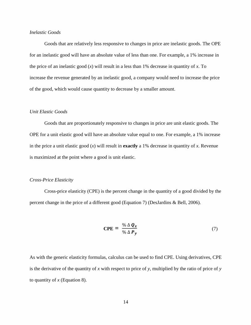
Cross-Price Elasticity
Cross-price elasticity (CPE) is the percent change in the quantity of a good divided by the
percent change in the price of a different good (Equation 7) (DesJardins & Bell, 2006).
CPE = % ∆ 𝑸𝒙
% ∆ 𝑷𝒚 (7)
As with the generic elasticity formulas, calculus can be used to find CPE. Using derivatives, CPE
is the derivative of the quantity of x with respect to price of y, multiplied by the ratio of price of y
to quantity of x (Equation 8).

15
CPE = 𝝏 𝑸𝒙
𝝏 𝑷𝒚∗
𝑷𝒚
𝑸𝒙 (8)
CPE has three interpretations: substitutes, compliments, and independents.
Substitutes
Substitute goods are those with positive CPE. If the price of good y goes up, the quantity
of good x will also go up. For example, if a soft drink company raises the price of their product,
the quantity sold of a second soft drink company's product that is a substitute good will increase.
The higher price of the first company's drink will cause consumers to purchase more of the
substitute good.
Compliments
Compliment goods have negative CPE. If the price of good y goes up, the quantity of
good x will go down. An example is if the price of french fries were to increase, the quantity sold
of hamburgers would decrease if french fries and hamburgers were compliments. The higher
price of french fries causes consumers to purchase less of the compliment as well.
Independents
Independent goods have CPE that are equal to zero. An increase in the price of good y
causes no reactions from good x. Independent goods are completely unrelated.
16
Income Elasticity
Income elasticity (IE) is the percent change in the quantity of a good divided by the
percent change in the income of the consumers of the good (Equation 9) (DesJardins & Bell,
2006).
IE = % ∆ 𝑸𝒙
% ∆ 𝑰 (9)
As with the other elasticity formulas, calculus can be used to find IE. Using derivatives, IE is the
derivative of the quantity of x with respect to income, multiplied by the ratio of income to
quantity of x (Equation 10).
IE = 𝝏 𝑸𝒙
𝝏 𝑰∗
𝑰
𝑸𝒙 (10)
IE has two basic interpretations: inferior or normal. Normal goods can be further categorized as
luxury or necessity.
Inferior Goods
Inferior goods have a negative IE. Thus, as income rises, consumers will buy less of the
good. Generally, inferior goods are relatively inexpensive, non-staple foods such as generic
equivalents of brand-name foods.

17
Normal Goods
Normal goods have a positive IE. As income rises, consumers buy more of the good.
Normal goods can be further differentiated into necessities and luxuries. Necessities have an IE
of between zero and one. These are staple products such as food and clothing. Luxury items have
an IE of greater than one and usually include much more expensive products.
Opportunity Costs
Opportunity costs are the next best alternative to the chosen option. Put another way,
what is given up to receive something else or the opportunities given up by making a decision.
Linear Regression
Linear regression involves a linear dependent and independent variables. No log
transformation is applied so linear regression is the regression of the raw values of the dependent
(y) variable on the raw values of the independent (x) variable(s). The coefficient(s) that results
is(are) the marginal effect of the independent variable(s).
Log-Log Regression
Log-log models use the natural log transformations of the y variable and regress them on
the natural logs of the x variables. The coefficients that result are the elasticities of the x
variables. Log-log models are useful in dealing with data that may be skewed or not normally
distributed. Much higher education data is positively skewed because the population of the
United States is ever increasing. Thus log-log modeling has many benefits in higher education
studies.

18
CHAPTER II
LITERATURE REVIEW
The literature review chapter is broken into three main sections. The first will describe
human capital theory as a basic framework for modeling student college choice. The second
section will detail many previous studies into enrollment demand theory, specifically focusing on
elasticity studies. The final section will discuss differential tuition research as it affects student
demand and institutional revenue.
Human Capital Theory
The framework of human capital theory begins with the assumption that people consider
education as an investment in human capital. When the benefits to be gained from this
investment outweigh the cost of the investment, people will choose to attend college (Schultz,
1961; Becker 1962). Benefits are usually future wages to be earned or the wage premium
associated with the chosen education. Costs are the tuition, fees, and opportunity costs that arise
from enrolling in college (Canton & de Jong, 2005).
Students are faced with a choice upon graduating from high school: enter college or enter
the job market. If they go to college, they forego the salary they would receive during the time
they are in college. This is their opportunity cost of attending college. They also pay direct costs
such as tuition, fees, and living expenses. However, they are able to add to their knowledge,
skills, attitudes, and talents, which can enhance their productive capacities and enable them to
become more sought after in the job market (Becker 1993; Woodhall, 1995). They will receive
higher salaries than their counterparts that did not invest in their human capital. This difference

19
equates to the wage premium of attending college. If high school graduates go to the job market,
they forego the wage premium, but they begin earning a salary at an earlier date.
The wage premium that exists between the salaries of high school graduates and those of
college graduates is quite large and has for the most part risen over time. In 1971, the wage
premium on after-tax earnings was 40%. In 2008, that number had risen to 60% (College Board,
2010). Research has shown that the premium will also increase throughout the working life of
individuals (Murphy & Welch, 1989; McMahon & Wagner, 1982). Lifetime earnings show even
greater differentiation. In 2008, college graduates with a bachelor's degree could expect to earn
66% more over their lifetime than high-school graduates (College Board, 2010).
Human capital theory assumes that students will engage in rational behavior. Students
behave rationally if they make choices about their resource allocation according to their budget
in a manner that maximizes their utility or satisfaction (DesJardins & Toutkoushian, 2005;
Paulsen & Toutkoushian, 2008). Students that follow rational investment decision criteria will
choose to go to college if the value of college, usually the value of the wage premium, is greater
than the direct costs (tuition and fees) and the opportunity costs (foregone salary) of going to
college (Corazzini, Dugan, & Grabowski, 1972).
It follows from the framework of human capital theory that students will find it more
attractive to invest in human capital when the economy is in a downturn. The opportunity costs
of education are lower because it is harder to find a job and salaries are lower. Thus, when
unemployment is higher, more people typically enroll in higher education (Bean, 1990; Saint-
Paul, 1993).
Human capital theory focuses on the relationship between the benefits and costs of
education. The costs include direct and indirect costs. Direct costs are tuition, fees, and living

20
expenses. The need to establish how institutions set tuition rates led Rusk and Leslie (1978) to
model tuition using a variety of variables including net costs, competitor prices, competitor
market shares, net income, and quality. They tested one state institution from each state and
found that 1976-77 tuition levels were linked to historical practices common to geographic
regions.
Prices at the universities were highly correlated with competitors' prices, both in-state and
in adjacent states. However, adjusting state appropriations was the major way to affect the level
of tuition. Rusk and Leslie concluded that tuition levels appeared to be the result of an
evolutionary process rather than a concentrated planning process (Rusk & Leslie, 1987).
While most scholars believe that education follows a human capital model as discussed in
the previous section, some evidence exists for viewing education as a consumption good as well
as an investment. Becker and Waldman (1987) examined the demand for higher education based
on a student's utility function. A portion of the student's utility arises from the wage premium
that they are striving for with an education, but a significant part of utility comes from the
"experience" of college. This consumption value includes friendships, sporting events, parties,
and other outside activities, but may be limited to undergraduate students as graduate or
professional students are more interested in furthering their education (Quinn & Price, 1998).
While it is difficult to quantify the value of consumption variables, Gullason (1989) used the
ability of male students in the 1960s and 70s to avoid the draft by going to college as
consumption good. He found that consumption goods have an empirically positive outcome on
undergraduate enrollment. Quinn and Price (1998) followed Gullason's work using the draft as
an explanatory variable for medical school enrollment, as well as a dummy variable indicating if

21
the U.S. was at war (during time periods of Korean and Vietnam Wars). They found that adding
consumption variables did not significantly affect medical school enrollments.
Human capital theory demonstrates that increasing the benefits of going to college or
decreasing the costs of attending will affect a student's likelihood of attendance. Thus, variables
that affect the cost or benefits are important factors in assessing demand for enrollment. The
wage premium associated with higher education is the main benefit and will be included in the
demand analysis in this study. Cost variables included will be direct costs and indirect costs of
attending college such as tuition, fees, interest rates, and unemployment. Consumption theory
indicates that modeling undergraduate students' demand may require using consumption
variables to be accurate. The difficulty in obtaining usable consumption variables may limit their
practicality in this study.
Enrollment Demand Elasticity
Enrollment demand elasticity studies have been conducted for approximately 50 years.
They can be ordered in several ways, such as data, level, or statistical methodology. The
following section will further break the literature on enrollment elasticity into several parts. The
first will be a discussion of several meta-analysis works on enrollment elasticity. These works
contain summaries of previous literature. The second section will discuss individual studies that
occur on the national level. Institution level studies will follow. The last section will cover
several miscellaneous projects that complete a robust review of the current literature.

22
Meta-analysis Studies
The first review of elasticity studies was Jackson and Weathersby (1975). The authors
reviewed seven studies conducted between 1967-75 to compare their quantitative results. The
results of these early studies show that own-price elasticity (OPE) is negative and usually
inelastic. The price effect ranged from -.06 to -1.9 % response to a $100 increase in tuition. The
seven studies also generally found income elasticity (IE) to be positive and greater than one,
indicating education was a luxury good. The authors found that across all studies, the income
effect became less as income increased. Another finding was the high negative correlation
between enrollment and net cost. Thus, increasing student financial aid does improve access to
higher education.
The major influence of the Jackson and Weathersby (1975) paper was the development of
a method of comparing results across the variety of research in higher education finance. Many
different data sets, functional forms, statistical estimations, and conceptual approaches are used
in the field and a method of comparison is necessary. The authors created a standardized
"typical" individual. This person had an income of $12,000 in 1974 and faced a college cost of
$2,000 per year. The participation rate was set at 26.2% of the eligible population being enrolled
in college. This allows calculation of the change in enrollment predicted by a $100 increase in
tuition.
Elasticity was defined as the percent change in quantity (change in enrollments per
eligible population divided by enrollments per eligible population) divided by the percent change
in price (tuition cost) as shown in Equation 11. Using the "typical" student, the percent change in
tuition cost is $100 (the predicted increase in tuition) divided by $2000 (the actual cost), so
(∆C/C) = (100/2000) = .05. (E/P) is the base participation rate of 26.2%.

23
OPE =
∆(𝑬𝑷)
𝑬/𝑷∆𝑪
𝑪
(11)
Rearranged, the formula shows that to find the change in enrollment per population (∆(E/P) for
each study would equal the elasticity times the cost ratio and the participation ratio as shown in
Equation 12.
∆ (E/P) = 𝑶𝑷𝑬 (∆𝑪
𝑪) (
𝑬
𝑷) (12)
Thus, any study that produces an OPE can be converted to a comparable student price response
coefficient (SPRC). The seven studies in Jackson and Weathersby (1975) had SPRC that ranged
from -.06 to -1.90, indicating that a $100 increase in tuition would result in a drop of attendance
that ranges from .06 % to 1.9%.
A second review of demand studies was conducted by Leslie and Brinkman (1987).
Using the SPRC technique developed by Jackson and Weathersby (1975) and correcting for
errors in the original authors mathematics, Leslie and Brinkman calculated SPRCs for 25 studies,
including those from Jackson and Weathersby. The data was converted to 1982-83 dollars to
allow for comparable analysis. The authors acknowledge that different studies present different
omitted variables that make comparison difficult. Any meta-analysis of demand functions with
such a variety of variables, forms, and specifications must simply rely on well-designed studies.
The results were similar to those found in Jackson and Weathersby (1975). All the
SPRCs are in the expected direction, enrollment declines when tuition rises. The mean response
was 2.1 or if tuition were raised by $100, enrollment would be expected to drop by 2.1%. The

24
results vary and many of the studies are lower than the mean. The modal results was 1.8%.
Studies with private universities generally showed lower SPRCs than public universities, most
likely due to the higher average family incomes of students attending private schools and the
higher general costs of such schools. SPRCs for community colleges was above the mean, which
is expected as students' responsiveness should be greater in a low-cost environment.
Heller (1997) updated Leslie and Brinkman (1987) by looking at the studies that had
appeared in the intervening decade. Heller found results that were consistent with Leslie and
Brinkman. SPRCs were found to be between -1.5 and -3.0, so that a $100 increase in tuition
would lead to decreases in enrollment of 1.5% to 3%. Heller also found that decreases in
financial aid lead to decreases in enrollment. As with Leslie and Brinkman, Heller's results
showed that lower-income students are more sensitive to changes in tuition than upper-income
students, and community colleges were more sensitive than public four-year schools or private
schools. Heller was able to analyze racial differences due to several studies estimating different
demand curves for different races. He found that Black students were more sensitive to changes
in tuition and aid than White students were, but information on Hispanic students was
inconclusive.
A fourth meta-analysis study looks at the variety of tuition and income elasticity studies
and treats the elasticity estimates as dependent variables and the attributes of each study as the
independent variables (Gallet, 2007). The study is designed to inform policymakers and
researchers which modeling procedures are most impactful in determining elasticities. The data
used was a collection of 60 different enrollment elasticity studies drawn from several literature
reviews including the three listed previously. The mean OPE of the studies was -.60 and IE was
1.07. Standard deviations were 1.00 and 1.97, respectively.

25
Results show that tuition elasticity is more inelastic in the short-run than in the long-run,
consistent with economic theory. The use of the linear functional form tends to result in more
elastic estimates when compared to the log-log form. Studies that use state or local data are more
elastic as are U.S. results compared to the rest of the world. There were no significant differences
in using cross-sectional versus time-series data. Non-white students' demands are generally more
elastic than students are in general. Many other characteristic variables such as gender, level, or
residency status are not statistically significant in regards to influencing tuition elasticity.
National-level Studies
Arguably, the most influential study of higher education demand was one of the first. In
their 1967 paper, Campbell and Siegal measured over the period 1919-64 the ratio of
undergraduate enrollment in four-year institutions to the number of 18-24 year olds with a high
school diploma and not in the military. This was a more accurate measure of the enrollment rate
in higher education than using the standard ratio of enrollees compared to the entire 18-24 year
old age group due to the Select Service draft during this era. The authors chose to model
enrollment demand based on disposable income and average real tuition. Statistically, those two
variables accounted for 87% of the variation in the stated enrollment ratio. From this analysis,
the authors found a price elasticity of demand or own price elasticity (OPE) of -.44 and an
income elasticity (IE) of 1.2 (Campbell & Siegel, 1967). In other words, a 10% increase in the
price of tuition would result in a 4.4% decrease in enrollment, while a 10% rise in income would
increase enrollment 12%. That means that student enrollment demand was inelastic or relatively
unresponsive to changes in tuition prices. The high IE was consistent with a luxury good. The
signs of the elasticities were notable. Economic theory predicts that OPE will have a negative

26
sign or as price goes up, quantity goes down, which was what Campbell and Siegal found. The
positive sign on IE was also expected for higher education as it is accepted as a normal good.
With a normal good, as individuals’ income rises, they consume more of the good.
Campbell and Siegel’s work is important for several reasons, not the least of which in the
pioneering nature of the study. Empirically, the use of a log-log (log-linear) functional form for
the regression is worth investigating. Regressions are calculated in a variety of manners, but the
log-log form is more easily interpreted when calculating elasticities. OPE is the percent change
in quantity of a good divided by the percent change in price of the same good. The linear
functional form in a regression gives a coefficient for tuition that is equivalent to the marginal
effects of the linear model. The individual elasticity will depend on the data set. Using the log-
log functional form transforms the data to logarithms. A result is that elasticity is now constant
over all the values of the data set. The tuition coefficient is now the elasticity itself, not the
marginal effects. A log-log functional form does not require any additional work to compute the
elasticity. The coefficient is the elasticity, thus results can be reported in a consumer-friendly
manner.
At the end of World War II, many soldiers took advantage of the G.I. Bill to attend
college. As many as 50% of the college students that enrolled between 1946 and 1949 were
financed by the G.I. Bill making college very inexpensive. Inexpensive goods are sometimes
thought to be inferior goods, or have a negative IE. Galper and Dunn (1969) investigated the
sizable negative effect the continuation of the military draft had on the demand for higher
education in the years after World War II. Increasing the size of the military invariably leads to a
decrease in the number of students going to college. Using the same data set as Campbell and
Siegel (1967), the authors found the elasticity for enrollment with respect to the size of the armed
27
forces to be -.26. Thus, an annual growth rate of 10% in the armed forces would decrease college
enrollments by 2.6%. Income elasticity was .69, making higher education a normal good despite
the inexpensive tuition (Galper & Dunn, 1969).
Beginning in 1947, there was a decline in the ratio of students enrolled in private colleges
versus public universities. Hight (1975) investigated this shift to determine the elasticity of
public and private education. Estimated OPE for private schools was -.71 while public schools
had an OPE of -1.78. Public schools were more elastic thus more responsive to changes in
tuition. More importantly, the IE for private schools was significantly greater than public. This
should imply that rising family income in the decades after World War II would have resulted in
an increase in the private to public enrollment ratio. However, Hight suggests that increases in
tuition at private schools resulted in much higher costs in comparison to public institutions,
dwarfing any impact of rising income.
Demand studies have for the most part tried to estimate the effect of tuition increases on
enrollment, but Savoca (1990) looked at the effect on the decision to apply. Using a two-step
maximum likelihood procedure, Savoca estimated a model with cost, quality, income, and a
matrix of other variables as the independent variables. The resulting coefficient and elasticity
were similar to those found in strict enrollment studies. However, if the school's tuition policy
and admission policy are independent, then the OPE for true enrollment is actually the sum of the
OPE for enrollment and the OPE for application, making the true OPE higher than the estimates
reported in the literature.
McPherson and Schapiro (1991) investigated demand from the viewpoint of net costs.
Their study looked at time-series data from 1974-84 and modeled demand as a function of net
cost (tuition minus financial aid), gender, and income levels. The data used was from the Current

28
Population Survey in which there was not enough years of data to allow time-series analysis for
Blacks or Hispanics, thus the analysis is for White students. They find that a $100 increase in net
cost leads to a 1.6% (adjusted for inflation) decline in attendance for low-income students. No
significant corresponding decline is found for high or medium income students. This indicates
that estimating different demand equations for different income levels might be a better approach
than simply using income as an independent variable.
The conventional method of describing the relationship between tuition and enrollment is
the theory of demand. As such, the higher the tuition of an institution, the fewer people will
choose to enroll in that institution. However, signaling theory postulates a different idea.
Signaling is the hypothesis that a higher rate of tuition signals potential applicants of the high
quality education offered by the institution (Spence, 1973). This is similar to the idea of Giffen
goods, goods that have a positively sloping demand curve. Giffen goods are theoretical goods
that consumers will purchase more of when the price of the good increases (Dougan, 1982).
Bezmen and Depken (1998) test the signaling hypothesis using demand for 772 U.S.
colleges. The signaling model of education states that a person’s productivity is identifiable by
the time they spent in school, but not increased by the time spent in school. In other words, a
more educated worker might receive higher pay because they hold a degree rather than because
they work better. The implication is that education is more credential based than skill based and
thus where a person receives their education is as important as what is the education.
Bezmen and Depken’s model is unique in that in addition to income, unemployment rate,
and a variety of characteristic variables (similar to other demand studies), Bezmen and Depken
include both in-state tuition and out-of-state tuition as a test of signaling. Higher tuition prices
are a measure of signaling in that higher quality education can be promoted by charging more.

29
Using a log-log functional form, the model for public schools returns estimates of in-state OPE
of -.018 and out-of-state OPE of .29, both statistically significant. This implies that institutions
that engage in signaling of quality to their applicants will be achieving the best results with out-
of-state students. The opposite seems true for in-state students. This result could be accurate for
out-of-state students, but the in-state result could also come from a large number of students
wanting to attend school close to home.
Several studies on private higher education institutions have found OPE for enrollment to
be positive or enrollment as a Giffen good. O’Connell and Perkins (2003) studied liberal arts
colleges in 1996. They built a model that included price, but also included some consumption
variables, following Quinn and Price (1998) and Gullason (1989). The resulting OPE ranged
from .017 to .366. All were positive, which is a characteristic of Giffen goods. Thus, the results
indicate that if these colleges raise price, their enrollment will actually increase. Clotfelter (1991)
used a similar model on 24 selective universities for the years 1981-88. He found positive
impacts of tuition on enrollment or applications. Both sets of authors conclude that reputation
has more of an impact on enrollment than does tuition cost for private institutions.
Noorbakhsh and Culp's (2002) project involving Pennsylvania public higher education
institutions analyzed in-state versus out-of-state tuition. In the 1990s, Pennsylvania adopted a
"full-cost recovery" program for non-residents. Non-resident tuition more than doubled in a six-
year period. Consequently, non-resident enrollment had fallen nearly 40%. The authors modeled
demand for non-resident and resident students in an effort to provide factual evidence for
policymakers. The models used were log-log forms with first-time freshman enrollment as a
function of institution tuition rates, competing institution rates, and income. Non-residents had
an OPE of -1.15, meaning their OPE is elastic. Resident students had an OPE equal to -.37. The

30
results showed non-resident students to be far more elastic in their demand and thus much more
responsive to a higher tuition rate. A second result was that IE for non-residents was 3.8 and was
significant at the 5% level. Residents had a non-significant IE of .4. Thus, non-residents have a
normal, luxury demand with respect to income. Pennsylvania's use of "full cost recovery" tuition
policies for non-residents sent many of those students to other states. Subsequent legislative
sessions revoked some of the language on non-resident tuition and allowed universities to set
tuition within a more reasonable prescribed range (Noorbakhsh & Culp, 2002).
Elasticities can be used to compare different classifications of consumers. One method of
differentiating students in an elasticity study is to compare students that apply for financial aid
with students that do not apply for aid. Students who apply for aid should have a more elastic Ed
because they are much more likely to be affected by tuition increases. Parker and Summers
(1993) used a pooled time-series method to look at liberal arts college matriculation rates. They
estimated demand curves for students that received aid, students that applied and qualified, but
did not receive aid, and students that did not apply for aid. The OPE for the non-aid students was
-.3 to -.36,while the aid students was -.29 to -.48, meaning students that receive aid are more
sensitive to changes in tuition, but only marginally so.
A study extending Parker and Summers work on the differences in elasticity between
students with financial aid and those without is found in a 2004 paper from Buss, Parker, and
Rivenburg on liberal arts colleges that analyzed over 100 schools using cost variables, aid,
quality, and macroeconomic variables. Data was split into aid applicants and non-aid applicants
and an OLS model was estimated for each using multiple functional forms. Non-aid applicants
had an OPE that ranged from -.6 to -.76, comfortably inelastic. Aid applicants had OPE between -
1.18 and -1.27, confirming that students who apply for financial aid are more responsive to

31
changes in tuition. Furthermore, gross tuition levels are found to matter more to students than net
cost (tuition minus aid). One explanation is that students look beyond the net cost and consider
tuition and aid separately because they are uncertain about continuation of aid over four years of
college (Buss, et al., 2004).
These two studies show how small differences in the models can result in very different
elasticity calculations. The Parker and Summers (1993) study did not include any
macroeconomic variables such as income or interest rates. It also included six measures of the
quality of the institution. The Buss (2004) paper included interest rates and income as well as a
time trend variable. It also included twelve quality variables as well as multiple measures of
competitor’s prices.
One aspect of state budgetary policies that is underappreciated is the contribution of
community colleges or two-year institutions to state education. Many times these are the first
institutions to feel the budget cut. In 2009-10, the California State Legislature leveled a $520
million (8%) cut on the California Community College system. In 2010-11, the legislature
proposed additional cuts of $400 to 800 million (6- 12%) (Californian Community Colleges,
2011). A study by Hilmer (1998) makes the case that states should be increasing funding to
community colleges in eras of budget cuts. During 1991-92, the average expenditure for a full-
time undergraduate at a four-year institution was $19,403. A student at a two-year cost $5,737.
Hilmer used an ordered probit model to test the CPE of two-year and four-year schools. He
found that increasing fees at a two-year institution caused enrollment to increase at four-year
schools and vice versa. Thus, the institutions are substitute goods with a positive CPE. The
difference was that the magnitude was ten times greater for two-year schools than for four-year
32
schools, meaning two-year institutions are far more responsive to changes in prices at four-year
schools.
Two of the most important studies for the current research project to consider were
conducted by Shin and Milton (2006, 2007). Shin and Milton (2006) studied the effects of tuition
level on enrollment in public colleges over the time period 1998-2002. They used all U.S. public
colleges with yearly enrollment data for the period considered for a total of 436 colleges. The
dependent variable was the number of in-state, first-time freshman enrollees. Shin and Milton
chose to include not only own-price effects (tuition and fees), but cross-price effects
(competitor's tuition). They also included wage premium as a measure of the future benefits of
college. Unemployment rates were added to examine the opportunity cost of college, while
financial aid was included to test a measure of net cost. Shin and Milton used many components
of previous studies, but were the first to combine all the above aspects into a single study.
The hypotheses postulated by Shin and Milton included the following: tuition will have
no effect on enrollment growth, competitor's price will have a positive effect on growth, and the
wage premium will have a positive effect on enrollment growth. A hierarchical linear model
(HLM) was used to allow description of changes over time in time-series data. Shin and Milton
used HLM because they were more concerned with the changes over time or a growth analysis
than in elasticity measurement.
As they expected, tuition had little effect on enrollment. The best estimate was that
colleges would have a 1.13% decrease for an increase in tuition. This is much lower than many
of the comparative studies such as Leslie and Brinkman (1987), Heller (1997), or Dynarski
(2000) who found decreases in tuition resulted in 3-5% increases in attendance. Enrollment was
much more sensitive to changes in competitor's prices. Private four-year institutions had a
33
positive CPE, while public two-year institutions had a negative CPE. Thus, enrollment in public
four-year schools was more responsive to changes in competitor's prices than to changes in their
own tuition rates. Wage premium also had a positive effect. Colleges in states with 1% higher
wage premiums had on average 4.25% more enrollment growth each year than colleges with
average wage premiums (Shin & Milton, 2006).
Shin and Milton's (2006) first paper is important to the current research in that it
establishes the wage premium and competitor's price as needed variables. The finding that an
institution's own tuition level does not influence its enrollment growth is intriguing and might
induce administrators to raise tuition at a more frequent rate. However, the authors do admit that
different time periods and different tuition ranges might lead to different results with respect to
tuition responsiveness.
The second paper by Shin and Milton (2007) is unique among the literature in that it
explores student responses to tuition increases at the college major level. The premise is that
state policymakers are more willing to tie tuition to cost of education, a so called cost-related
tuition policy. While this is not true differential tuition, it is worth examining. With a cost-related
tuition policy, actual college costs are important. Costs will differ by credit hour, major, level of
student, etc. To determine what to charge in such a system, student's responses to tuition changes
must be analyzed.
To that effect, Shin and Milton (2007) modeled enrollment as a function of current
tuition, tuition changes, other school costs, financial aid, instructional expenditures, and student
dormitory capacity. The population of data was all public four-year colleges and universities in
the U.S. that reported institutional-level data on the dependent and independent variables. An
OLS method was used with a log-linear functional form, thus the coefficients can be interpreted

34
as the proportional change in enrollment caused by a one unit change in the independent
variables (Shin & Milton, 2007).
Tuition levels were reported in the overall model with a coefficient of -.011 for 2004
costs. That means that a $100 increase in tuition will result in a 1.1% decrease in enrollment.
These results are significantly less than those reported in Leslie and Brinkman (1987) and Heller
(1997), but consistent with previous work by Shin and Milton (2006).
There were significant differences across the selected majors. Physics (-.005), Biology (-
.009), and Business (-.013) showed negative responses to tuition increases. Enrollment in
Physics would decrease .5% with an increase of $100 in tuition. Biology enrollment would
decrease by .9% and Business by 1.3%. All three were significant at the .05 level. Engineering,
Math, and Education had very small negative or even positive coefficients, but none were
significant. Shin and Milton (2007) postulated that those majors with high rates of return would
not be sensitive to tuition. The results tend to support this hypothesis. Engineering students, the
discipline with the highest rates of return, were not sensitive to tuition increases. Biology,
Physics, and Business students, those with medium rates of return and medium costs to the
university, were sensitive to changes in tuition price. Education, with lower rates of return and
lower costs, were also not sensitive to tuition increases, but the results were not statistically
significant.
Shin and Milton (2007) analyzed student's response to tuition changes across majors or
colleges. Their study looked at several hundred institutions in the U.S. in terms of cross-sectional
data. Further analysis at a single institution using a time-series analysis will provide more
information.

35
Institutional-level Studies
The higher education community functions similar to a monopolistically competitive
market, with many firms that each have a differentiated product. Each faces competition from all
points and while each is producing education as its commodity, there exists a niche market for
each institution. That niche gives each college or university some semblance of control over
prices. Estimating demand for enrollment on a national or even regional level may not be the
best method of determining what is happening at a single institution. Thus, it is useful to estimate
demand at individual institutions. The nature of competition among higher education institutions
can be quantified by estimating a demand for enrollment that includes competitor's prices as an
independent variable. This results in a measure of two institutions’ relationship referred to as
cross-price elasticity (CPE).
One of the first institution level demand study was conducted in 1977 using data from the
University of Hawaii (Ghali, Miklius, & Wadak, 1977). The model developed estimated
enrollment based on cost, income, ability, gender, family size, and the type of high school
attended. Results showed an elasticity of demand (OPE) equal to -.476, which is inelastic.
Hawaii's geographic isolation and low level of tuition in the early 1970s could have contributed
to students’ relative indifference to tuition changes. Cross-price elasticities between the
University of Hawaii and several competitors across a range of institutional types (two-year,
four-year, public, and private) were close to zero and little significance, meaning there is little
true competition for the University of Hawaii (Ghali, et al., 1977). The implications are that a
significant increase in tuition will not cause a significant drop in enrollment, making the
University of Hawaii a logical candidate for increasing revenues by increasing tuition.

36
Similar studies were conducted for Cornell and Occidental College in the 1980s. The
study done for Cornell students looked at categories including family income, SAT score, and
legacy and estimated the demand for enrollment with respect to the two components of the
Cornell system, statutory colleges (colleges that are part of a private institution that receive state
funding) and endowed colleges (privately funded colleges within a private institution). All of the
elasticities for the statutory colleges were inelastic with the overall being -.28. The endowed
elasticities range from -.41 to -1.58, with the overall at -1.09 (Ehrenberg & Sherman, 1984).
Thus, students attending the endowed colleges were far more sensitive to changes in the price of
tuition.
Moore, Studenmund, and Slobko (1991) found similar results at Occidental. Using a
model that included personal variables such as race, gender and legacy and cost variables, they
estimated the enrollment demand using a logit model. They found that the OPE for students that
applied for financial aid was -.72, while students that did not apply for aid had an OPE of -.35
(Moore et al., 1991). Both results are inelastic, but students that apply for aid have a relatively
more elastic demand. They will respond more to changes in price and with federal grant money
trending downward, are less likely to attend. This may force private schools like Occidental to
give them some incentive to attend by increasing private grants and scholarships.
In their 1999 paper, Allen and Shen employed a simple demand model to test the
environment of competition that exists around small, regional private schools. Their model
includes as competitors, a public, comprehensive university within the same area, a public,
research university within the same state, and a private university in a neighboring state. Using a
log-log functional form, the authors find an income elasticity (IE) of 1.7 and cross-price
elasticity (CPE) between the private institution and its nearest private competitor of .51. The data

37
shows this institution to be a normal, luxury good (IE > 1) and the two schools together to be
substitutes (CPE > 0). Of note, the CPE of the institution of study and the public universities was
minute and insignificant, indicating that the true competitor for this private institution is its
fellow private school.
Even more interesting, the OPE for the private institution without including competitors
is -.64. Adding the three competing schools increases OPE to -1.09 (Allen & Shen, 1999). Thus
adding competition transforms the enrollment in the private institution from inelastic to an elastic
good. Without competition, students are not responsive to changes in tuition price. The addition
of competitors changes the equation. Competition becomes a limiting factor on revenue
generation.
Vasigh & Hamzaee (2004) studied enrollment demand for undergraduates and graduates
across two campuses of a private institution. Using a log-log functional form, enrollment is
estimated as a function of tuition, income, unemployment, and financial aid. Tuition costs seem
to have no impact on enrollment, with some of the OPE actually being positive, indicating
potential Giffen goods. Undergraduate OPE ranged from .07 to .44, while graduate ranged from -
.24 to .53. An increase in publicity and rank could be a cause of the positive, seemingly Giffen
elasticities, as could growth in the industries served by the institution.
Most of the previous studies done on tuition pricing have focused on student's ability to
pay, financial aid availability, or college costs. Bryan and Whipple (1996) analyzed the student's
willingness to pay. To achieve this result, they asked current students at Mount Vernon Nazarene
College (MVNC) a series of questions pertaining to their responses to hypothetical tuition
increases. Choosing six elasticities (ranging from -.03 to -.49) from surveys and previous
literature, the authors calculated the projected net earnings for MVNC for each scenario. The

38
findings were very informative. At low tuition prices of $6000 per semester, student's demand
was highly inelastic. They were very likely to remain at MVNC at those prices, but university
earnings were low ($28,885). When prices moved to a mid-range, $7000 per semester, students
begin to look for more options and demand became more elastic, however enough students
stayed at MVNC for earnings to reach $595,052. As prices reached the highest level,$8000 per
semester, demand was much more elastic and MVNC's earnings fell dramatically ($-273,791).
The implications of this paper are clear. Applying the earnings and elasticity model to
private colleges should allow those colleges to find a tuition level that will generate the highest
possible revenue. One question administrators must ask however is if high net earnings is the
only goal of the institution. Most higher education establishments, especially small privates, may
have other goals. Balancing economic realities with educational goals is the ultimate question in
higher education.
Curs and Singell (2010) investigated enrollment demand as part of a tuition/aid study at
the University of Oregon. The authors used net price, instead of tuition, in order compare price
responsiveness across groups. The unique aspect of this study is that the authors divided
applicants into nine categories covering need and ability. They estimated elasticities for each of
the nine categories. Elasticities became more inelastic as the student moved from non-needy to
needy and from less able to more able. Thus students with little need for aid, but with less ability
were more responsive to price changes and more likely not to enroll if net prices were higher.
Students with great need for aid or with great ability were more likely to enroll regardless of the
net price. This could be because students with great need were likely to have the same net price
regardless of institution. Since the majority of need-based aid is Federal funds, those funds can
follow a student to any institution they choose to attend. If they received an increase in funds

39
available for the University of Oregon, they would be able to receive a similar increase at
Oregon State. For those students that had little need for aid, price changes at the University of
Oregon would have more of an impact because they do not receive funding at all potential
choices.
Demographic Based Studies
Some papers have attempted to include racial data in elasticity studies. McPherson and
Schapiro's (1991) results showed that White, low-income students were more affected by tuition
changes, but they did not have the data to look at Black or Hispanic students. Cameron and
Heckman (2001) looked at minority students within a large-scale project encompassing more
than costs. They did not measure elasticities, but did model academic attainment for Black,
Hispanic, and White males to investigate the sources of racial and ethnic disparity in college
attendance. When controlling for family background, minorities are more likely than Whites to
graduate from high school and attend college. Tuition has only a limited effect on minority
attendance, but what the authors term "early differences in resources" are the main cause of
differences in White and minority enrollment. Family income is important, but not for the
obvious reason of ability to pay for college. Income is more important in establishing a desire
and need to attend college and in preparing a student for college. The authors argue for more
funding for high-school education and preparedness than for increased federal loan programs as
a way to increase minority college attendance and success (Cameron & Heckman, 2001).
Another study discussing differences in elasticity due to race is Wetzel, O’Toole, and
Peterson (1998) which estimated the enrollment demand at Virginia Commonwealth University
VCU) based on ethnicity. The study uses net cost (tuition minus aid) as one of the independent

40
variables. The enrollment yields at VCU are relatively insensitive to changes in net price.
However, unlike the previous study from Cameron and Heckman, Wetzel, O’Toole, and Peterson
did measure elasticities and found that Black students are two thirds more responsive than White
students to changes in net cost. The implication is that increases in financial aid to Black students
could dramatically increase enrollment yields.
Kane (1994) used the methodology pioneered by Jackson and Weathersby (1975) and
used in Leslie and Brinkman's (1987) meta-analysis paper to show student's price responsiveness
to tuition changes for black and white students in different income levels. Leslie and Brinkman
found that the papers they studied showed a $1000 decrease in the net price of schooling caused
a 3 to 5% increase in attendance. Kane found that the responsiveness varied greatly between
black and white students and between income levels. In the bottom quartile of income levels, a
$1000 increase in costs would decrease black enrollment by 22.1% and white enrollment by
11.4%. In the highest quartile, black enrollment would still decrease by 13.2%, while white
enrollment would only fall by 1.7%. Black students were more responsive than whites to tuition
changes in all quartile.
Previous studies into elasticity of tuition have ranged from meta analysis over large
numbers of institutions to studies only affecting single private or public institutions. While many
of these studies provide information about elasticity, none provide the more detailed examination
that this paper will attempt. Shin and Milton (2007) looked at tuition response to individual
majors over a cross-section of universities, but they did not expand the study over multiple years.
Several studies have looked at individual universities over time, but not including examining
different colleges at those universities. This study will attempt to fill the gap between the two
types of studies that have been conducted in the past.
41
Differential Tuition
Differential tuition has been used as a method for increasing university revenues at some
campuses for many years, but was not in widespread use until relatively recently. Charging
different students different rates has led to concerns about access. Will charging higher tuition
for higher demand colleges or majors force low-income students to choose to major in lower-cost
programs because they are more inexpensive to attend? Nevertheless, many schools use some
type of differentiation and this practice will likely continue as higher education institutions seek
to diversify funding sources (Ward & Douglass, 2005). The continual decline in state support for
higher education has made differential tuition a viable option to be explored at public universities
to raise revenues (Heller, 2006).
Types of Differential Tuition
The most basic tuition differentiation is the different rates that undergraduates and
graduates pay. According to Saupe & Stephens in 1974, about 25% of the land grant universities
surveyed charged a different rate for graduate and undergraduates.. The authors state that
universities had begun to use different rates for graduate students because of the higher costs
associated with said graduate students. According to a 2010 survey, 91% of institutions charge a
different rate for graduate versus undergraduate levels (Simone, 2010).
A second form of tuition differential is that of state resident versus non-resident students.
This differential has been used more often than graduate versus undergraduate rates. A 1971
study indicated that tuition differentials for residency were widespread and substantial in all parts
of the country (Carbone & Jenson, 1971). Simone found that in 2010, nearly 99% of public four-
42
year institutions and 97% of public two-year institutions charge different rates based on
residency (Simone, 2010).
One method of determining tuition rates that has been considered is using class standing
(freshmen, sophomore, junior, and senior). This type of differentiation was in use in the late
1970s and early 1980s when it was reported to be in use at the University of Michigan,
University of Minnesota, and University of Washington (Yanikoski & Wilson, 1984). As the
student gets closer to a degree, the price elasticity becomes much more inelastic. This means the
student is willing to pay more at the end of a degree program than at the beginning and is more
unwilling to leave the same program. Increasing tuition rates to upperclassmen would
theoretically increase revenue and decrease costs for freshmen, increasing access. A study by
Chressanthis (1986) estimated demand at Saginaw Valley State College from 1964-1983. The
model included tuition, competitor tuition, housing, and unemployment. Different models were
estimated for different classes. The own price elasticity (OPE) for freshmen was -1.74, while
seniors had an OPE equal to -.59, showing the expected results of student's demand becoming
more inelastic as they advanced in classification. However, these results and the economic theory
behind this method of differentiation have still only led to less than 10% of schools charging
students with different classifications, different tuition rates (Simone, 2010).
Another method of differing tuition is charging students more based on peak load. Peak
load differentials involve charging lower rates during non-peak utilities usage to increase
efficiency of physical plant and increase classroom usage. With additional class times during
non-peak hours, demand was driven from peak times to a more broad range of hours. This
allowed a greater utilization of physical plant assets, more revenue per student, and savings of

43
capital expenditures by not constructing new physical plants based upon skewed peak loads
(Avila, 1972; Weinberg, 1978).
Most of these types of differentiation are not practiced by institutions around the
country. The most prevalent remain graduate versus undergraduate and residency differences.
Combining all factors other than residency, nearly 70% of institutions use at least one of these
factors to charge a different tuition level. Nearly one-third charge based on two or more factors
(Simone, 2010).
Politics of Differential Tuition
Initiating a differential tuition strategy is an exercise in politics. The public has been
accustomed to low tuition and low cost education financed through state and federal support
since World War II. This has generated a sense of entitlement to a low cost education regardless
of the rising costs involved (Ward & Douglas, 2005). In the U.S., the public is usually non-
responsive to the government decreasing funding of higher education, but the opposite is true if
tuition and fees are increased. This has led to much of the general public calling for higher
education to apply industry methods of cost controls and efficiency innovations in order to
maintain low tuition levels (Ward & Douglas, 2005).
The main factor contributing to the proliferation of differential tuition is the decreasing
amount of funding public institutions receive from state and national sources. There are three
main sources of funds for higher education instruction, tuition and fees, federal funds, and state
and local funds. Prior to the World War II, tuition and fees and state funds were much greater
than federal funding. The passage of the Servicemen's Readjustment Act (GI Bill) in 1944
increased enrollments and the amount of federal funding institutions received, spurring a massive
growth in education spending and revenues. From 1960 to 1980, revenues in higher education

44
increased over $50 billion or ten times the amount in 1960 (Heller, 2006). Of the three main
sources of revenue for higher education tuition and fees have risen at the fastest rate. State
appropriations have increased at the slowest rate. From fiscal year 2000 to 2004, state funds
increased only 6.5% per year, while tuition prices increased between 16% and 40% depending on
institution type. Percentages of total funding are even more telling. The percentage of total
revenue that was gained from state sources has decreased from a high of 34% in 1980 to 26% in
1996. The share of federal funding has declined in the same period from 15% to 12%(Heller,
2006). These numbers have continued to decrease. This decline has been offset by increases in
the share of tuition and fees. Tuition and fees have reached the point of generating about 30% of
the operating revenue of four-year public universities (Derochers, Lenihan, & Wellman, 2010).
While tuition increases and differential tuition can provide increases in revenue, they may
cut off access to low-income students. While the college-going rates have increased for all
socioeconomic and ethnic classes at the same rate over the past few decades, despite the
continuing differences in those ethnic college-going rates, the net cost of attendance as a portion
of income remains highest for the lowest income families. The net cost of attending higher
education institutions absorbs 45%, 38%, 30%, 20%, and 11% of the total annual income of
families in the five quintiles (Heller, 2001). Increasing tuition further will place a greater burden
on the lowest 60% of U.S. families that would need to spend from 30% to 45% of their annual
income to send their children to college. Problems with access can be helped with increases in
financial aid. The University of California raised tuition in the early 1990s but accompanied this
increase with an increase in the amount of aid given to low and middle income students.
Universities normally give $.25 in aid for every $1 in tuition raised. The University of California

45
raised this percentage to $.35 in aid for a $1 raised in tuition. The result was no discernible drop
in demand or in access (Ward & Douglas, 2005).
Another compelling argument for the introduction of differential tuition is making tuition
more equitable to students. In a flat rate tuition scheme, where all students pay the same amount,
students in low-cost colleges, such as education, have to pay for the education of students in
high-cost colleges, such as engineering. A differential tuition policy or cost-related tuition policy
would ensure that students in high-cost colleges would pay a higher amount, while those in low-
cost curricula would be charged less. There is some evidence that flat rate tuition plans are
actually regressive, reduce access, when compared to differential plans (Hansen, 1970;
Windham, 1972).
Rothschild and White (1995) developed a model of higher education pricing based on the
supposition that colleges provide human capital as an output and students are clear inputs. The
question is if there are pricing schemes that allow an efficient allocation of resources in a zero-
profit environment such as in higher education. The authors’ model yields intriguing
conclusions. First, different students may be charged different tuitions at the same university
because they may receive different amounts of human capital at the same university. Students of
the same type may receive different amounts of human capital from different universities, but
they will pay different tuitions at those universities so that the net gain will be uniform across
universities. Universities may use different technologies, admit different types of students,
provide different levels of human capital, and charge different tuitions, but the tuition and human
capital package that a university offers to a given student must meet the requirement for uniform
net gain across all students of all types.

46
Students that are charged a cheaper tuition rate for lower cost curricula will receive less
human capital and lower career earnings or wage premiums. Higher-quality universities that pass
on more human capital are able to charge more because their graduates will generate higher
future earnings. Rothschild and White (1995) present a competitive equilibrium model that
seems to explain the underlying reasoning for differential tuition. The authors admit however,
that real world pricing strategies do not resemble those in their model, possibly due to market
imperfections or technological differences.
The economics of colleges and universities have become more important as state funding
dries up. With a higher percentage of university revenues coming from tuition, differential
tuition rates become more attractive. Many universities offer differential rates of at least one or
two kinds, but not many choose to differentiate based on colleges. Charging higher amounts to
students that are earning degrees in fields that have higher wage premiums may be a way to
increase revenues. However, if there are no differences in elasticities, or price responsiveness,
across colleges, then universities may lose money and patronage by charging differential tuition.

47
CHAPTER III
METHODOLOGY
This chapter provides the mechanics of the study. The relevant research questions are
presented again and the research design is described. The research design section will include a
brief overview of the study as well as the following sections: the data to be analyzed and method
of collection, the model, and statistical methods. A summary will reassert the most significant
aspects of the design and set the groundwork for the results chapter.
Research Questions
The main objective of this study is to estimate demand for enrollment in different
colleges at State U. Demand for enrollment is estimated using a variety of determinants
including cost variables, personal characteristic variables, and macroeconomic variables. The
demand estimation will allow the researcher to calculate price elasticities (OPE) and income
elasticities (IE) for each of eight colleges at State U. Determining elasticities for each college
would give State U and government officials information on the relative tuition sensitivities by
college. Thus, the primary question is “What is the elasticity of demand for enrollment for
different colleges at State U and what are the implications for differential pricing in higher
education?” This main question can be broken down into the following five research questions:
Question 1: Do differences exist in the price elasticity of demand for different colleges?
Question 2: Does any college’s price elasticity of demand classify that college as having an
inelastic demand for enrollment with respect to tuition?
48
Question 3: Does any college’s price elasticity of demand classify that college as having an
elastic demand for enrollment with respect to tuition?
Question 4: Does any college’s price elasticity of demand change greatly over time?
Question 5: What is the estimated effect charging differential tuition rates according to
elasticities would have on State U’s general revenue and enrollment?
A secondary question is “What are the income elasticities for various colleges at State U and
how do changes in income affect enrollment?” There are four research questions for the
secondary question of the paper:
Question 6: Are there significant differences between colleges in income elasticities?
Question 7: Are any of the colleges considered luxury goods?
Question 8: Are any of the colleges considered necessity goods?
Question 9: Does any college’s income elasticity change over time?

49
Research Design
Overview
The researcher will address the above questions by analyzing historical enrollment data
from a flagship, land-grant university, State U. Data will be collected on the number of
applications for each of eight colleges at State U and used in an ordinary least squares (OLS)
regression to build a demand equation for enrollment in each college. The regression results will
provide the researcher the means to calculate price and income elasticities for each of the ten
colleges at State U. These elasticities will provide information about the differences across
colleges with respect to demand and potential revenue generation. The study will follow the
work of Shin and Milton (2007) by looking at individual colleges within State U, as they are the
only study to work in this direction.
Data
Data collected for the dependent variable will consist of the number of actual freshman
applications to State U over the time period 2003-2015. The decision to use applications instead
of freshman enrollment relates to the overall high demand for an education at State U. State U is
consistently a top ranked university, both nationally and internationally, and its status as a public
university and relatively low tuition make it one of the best values of any college in the United
States. The result is far more students applying for State U than are admitted and enrolled.
Consequently, enrollment, used in the majority of demand studies listed in Chapter Two (Vasigh
& Hamzaee, 2004; Ghali, et al., 1977; Moore, Studenmund, and Slobko 1991; Ehrenberg &
Sherman, 1984), would not lend itself to the most useful interpretation. Instead, this researcher

50
will use applications as the dependent variable as Bezmen and Depken (1998) did in their study
of signaling.
Independent variables to be used in estimating application demand are divided into two
main categories: cost variables and macroeconomic variables. The data required for the
independent variables is available from State U records as well as United States Federal Reserve
databases.
Variables
This study will entail the development of a time-series model for enrollment in each of
eight colleges at State U based on the number of freshman applications into those colleges. The
colleges are Agriculture and Life Sciences, Architecture, Business, Education, Engineering,
Geosciences, Liberal Arts, and Sciences. The theoretical model is shown in Equation 13, with
applications as a function of a set of cost variables and macroeconomics variables.
Applications = f (State U Tuition, State U Fees,
Two-Year Competitor Costs, Four-Year Competitor Costs, Income,
Unemployment Rate, Interest Rate, Wage Premium) (13)
Applications for the eight colleges are shown in Figure 3. Data was collected from
several reports presented by State U (State University, 2016a). Several of the colleges have a
relatively flat appearance when graphed in this manner. However, there is a legitimate increasing
trend in each college. There are several ambiguities though. First is the manner in which the
College of Agriculture tends to have plateaus in applications. From 2003 to 2009, applications

51
for the College of Agriculture go from 923 to 1254, a change of around 5% a year. There is a
rapid increase following this stagnation in 2010 – 2013 from 1254 to 2673, over 30% increases
per year, followed by stagnation in 2013-2015.
Figure 3. Applications in Eight Colleges at State U from 2003-2015.
Other colleges, such as Business, Liberal Arts, Education, and Architecture show more
standard linear progressions. Both the College of Science and the College of Geosciences show a
decrease in the years 2013-2015, while Engineering has an explosion in growth of applications
over the same time period.
0
1000
2000
3000
4000
5000
6000
7000
8000
9000
AG AR EN ED GE LA BA SC

52
Cost variables include both tuition and fee costs at State U and some competitor costs. In
order to calculate elasticities, some measure of the price of attending college is necessary. At the
majority of colleges, costs are divided into at least two components, tuition and fees. Tuition and
fees are included in the analysis independently to account for the potential of University
administration transmitting higher costs of education to students at State U in fees instead of
raising tuition costs. Gross tuition is used in order to study the effect of tuition increases on
tuition independent of aid. Tuition and fee data was collected from State U’s Student Business
Services website (State University, 2016b)
State U undergraduate students pay a flat rate for tuition and fees for any amount of hours
at full-time status (12 credit hours per semester) or above. Colleges and Departments can impose
their own fees for specific courses, but that data is unavailable. In the 2013-14 school year, this
amounted to $2648.25 for tuition and $1604.59 for fees for residents in those colleges that did
not have differential fees, not including parking fees or sports attendance fees. Four colleges,
Architecture, Business, Education, and Engineering, charged a varying fee to their students,
above and beyond state mandated tuition. By 2015, every college has different tuition schedules.
Figure 4 shows the changes to tuition over the past decade.

53
Figure 4. State U Tuition for Eight Colleges During Years 2003-2015.
$-
$500.00
$1,000.00
$1,500.00
$2,000.00
$2,500.00
$3,000.00
$3,500.00
$4,000.00
$4,500.00
AG AR EN ED GE LA BA SC
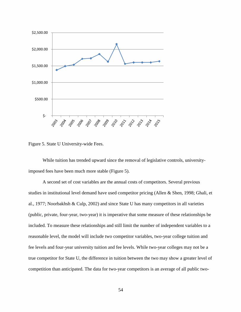
54
Figure 5. State U University-wide Fees.
While tuition has trended upward since the removal of legislative controls, university-
imposed fees have been much more stable (Figure 5).
A second set of cost variables are the annual costs of competitors. Several previous
studies in institutional level demand have used competitor pricing (Allen & Shen, 1998; Ghali, et
al., 1977; Noorbakhsh & Culp, 2002) and since State U has many competitors in all varieties
(public, private, four-year, two-year) it is imperative that some measure of these relationships be
included. To measure these relationships and still limit the number of independent variables to a
reasonable level, the model will include two competitor variables, two-year college tuition and
fee levels and four-year university tuition and fee levels. While two-year colleges may not be a
true competitor for State U, the difference in tuition between the two may show a greater level of
competition than anticipated. The data for two-year competitors is an average of all public two-
$-
$500.00
$1,000.00
$1,500.00
$2,000.00
$2,500.00

55
year schools in the state. Four-year data was taken from the average of State U’s three biggest in-
state, public competitors (State Higher Education Coordinating Board, 2016).
Figure 6. Four-year and Two-year Competitor Tuition Rates for 2003-2015.
Figure 6 shows the four-year and two-year costs. It is easily apparent that State U’s four-
year competitors have had increases in tuition similar to State U’s increases. What is interesting
is that the two-year college average has not increased at rapidly. There has been a steady increase
in the cost of two-year alternatives, but not on the magnitude of four-year.
The macroeconomics variables of interest include income, unemployment rate, interest
rate, and the wage premium. Three variables will be lagged one time period based on the idea
that students respond more slowly to changes in macroeconomic variables (Allen & Shen, 1998).
Therefore, 2010 student data would be matched to 2009 economic data. The interest rate will not
$-
$1,000.00
$2,000.00
$3,000.00
$4,000.00
$5,000.00
$6,000.00
4 Year 2 Year

56
as students apply for current loans not previous year loans. Income will be measured in the form
of the State U's state per capita disposable income (PCDI). Disposable income is total personal
income minus personal current taxes. PCDI is that measure divided by state population. Income
has been included in many demand studies and usually in the form of PCDI (Campbell & Siegal,
1967; Hight, 1975; Allen & Shen, 1998; Buss, et al., 2004). Including income allows the
calculation of the income elasticity for each of the ten colleges. This will indicate if enrollment at
each college is a normal or inferior good. Using State U's own state PCDI will allow a more
accurate estimate of income effects as in most state flagship schools, the great majority of
students are from within the state. Figure 7 shows the state's PCDI (U.S. Bureau of Economic
Analysis, 2016). As expected, this number has a large positive trend.
Figure 7. Texas PCDI for 2003-2015.
A second macroeconomic variable is the rate of unemployment. Unemployment is
measured as the unemployment rate in the state for each time period. Different states have
$25,000.00
$30,000.00
$35,000.00
$40,000.00
$45,000.00
$50,000.00

57
different responses to recessions and growth periods. Thus it is more useful to include the state
unemployment rather than the broader United States unemployment. Higher unemployment rates
may lead to higher enrollment rates in colleges. The lower opportunity cost, for example the
salary a student could have made as a full-time employee if he/she chose a vocation instead of
going to college, directly after high school results in more students foregoing work to consider
higher education (Chessanthis, 1986). However, a second observation is that the higher
unemployment rate could result in more parents being out of work and thus unable to afford to
send their child to college, particularly for State U which as a flagship is more expensive than
many of its competitors (Buss, et al., 2004). Texas’ unemployment rate is shown in Figure 8.
There are decided peaks and valleys in the 13 years of data. Obviously, recessions and periods of
growth in the economy spur unemployment.
Figure 8. Texas Unemployment Rate and Stafford Loan Rate.
0.0
1.0
2.0
3.0
4.0
5.0
6.0
7.0
8.0
9.0
TX Unemployment Rate Stafford Loan Rate

58
What is interesting is the relationship between unemployment and the third
macroeconomic variable, interest rate. Interest rates were included in the model in the form of
the Federal Stafford Loan Rate (Educated Risk, 2016). Higher interest rates tend to discourage
students from seeking student loans as a form of financial aid to pay for college. If a student
knows they will have to pay large rates on their loans, the opportunity cost of college becomes
higher. Similarly, with high interest rates, students could earn more money on their investments.
Investments made with money that would be spent on an education. This is the opportunity cost
of investment. The expectation is that the higher the interest rate, the lower the enrollment
demand, hence a negative relationship. As of May 2013, student loans outstanding were greater
than $1.25 trillion (Chopra, 2013).
Looking again at Figure 8 shows a distinctive pattern. In times of low unemployment,
when the economy is doing well, the loan rate is higher. This is because the Stafford rate is tied
to the U.S. Treasury Bill rate. When the economy is doing better, Treasury bills have a higher
return.
The final macroeconomic variable is the wage premium. Wage premium is the difference
in average salary of an individual that graduated from high-school and entered the work force
and an individual that graduated from college before entering the work force. Several studies
suggest that the wage premium is a major determinant of demand (Corazzini, Dugan, &
Grabowski, 1972; Becker 1993; Woodhall, 1995), but relatively fewer include it in tuition

59
demand estimations (Shin & Milton, 2006).
Figure 9. College Graduates Wages as a Percentage of High School Graduates Wages.
Wage premium is calculated for each year from United States Census Data and is
measured by the percentage of average income for those with baccalaureate degrees to the
average income for high school graduates. Data was collected from the U.S. Census Bureau
Current Population Survey 2016 and is shown in Figure 9. Wage premiums were unavailable for
the totality of the data set for each college. State U has begun collecting data on the starting
salaries of students from individual colleges and degrees, but this data is only available from
2011-2015. Eventually, inclusion of such data will make this study much more robust.
106%
108%
110%
112%
114%
116%
118%
120%

60
Tests for Stationarity
As shown in the graphs of the data, most of the variables appear to be non-stationary,
meaning that the series has a trend and does not return to its mean. Some data behaves like a
random walk; new information will change price levels in the short run but not affect the long
run mean. Other data series increase or decrease in a pattern or trend. Those trends are non-
stationary and make time series analysis impossible. All variables need to be tested for
stationarity and corrections applied to those that are non-stationary.
The test for stationarity is the Dickey-Fuller (DF) test. The null for the DF is that the
variable's data series is non-stationary. The alternative hypothesis is stationarity. The test for
each series is based on an ordinary least squares regression of the first differences of each
variable on a constant and one lag of the levels of each variable. The t-statistic is associated with
the estimated coefficient on the lagged levels variable from this regression. Under the null
hypothesis, the statistic is a non-standard t distribution. The critical values for the DF test for the
95% significance level is are -2.89(5%). The null will be rejected for any t values less than the
5% critical value (Fuller, 1976).
A Dickey-Fuller test was conducted on each of the eight colleges. An initial regression
was run to get the residuals for each model. The lagged residuals were used as the independent
variable regressed on the change in residuals, the dependent variable. The results of the DF tests
are shown in Table 1. All eight colleges had t-statistics less than -2.89 for the DF tests. This
means that each model, when taken collectively, is stationary. There are no statistically
significant patterns in the data. No adjustments, lags or corrections, need to be applied to the
models in order to run regressions.

61
Table 1
Dickey-Fuller Test Statistics
College T-statistic
AG -5.75
AR -3.92
BA -3.79
ED -5.19
EN -3.89
GE -4.25
LA -4.22
SC -4.67
Model
The variables listed above will be used as predictor variables in the estimation model.
The model will be estimated using a log-log and log-linear functional forms. Discussions on the
correct functional form end with varying conclusions. The log-log form produces results that can
be interpreted more easily as elasticities. In the log-log form, the coefficients on tuition price and
income will be the OPE and IE, respectively. However, the log-log form assumes elasticity is
equal across all levels of observation (Bezmen & Depken, 1998). The log-linear form assumes
that the effects of the independent variables are dependent on the size of the independent
variables (Shin & Milton, 2007). Coefficients on tuition price and income are interpreted as
proportional changes in applications caused by a specified unit change in tuition or income. Both
specifications will be tested to ensure robustness of the analysis.
The empirical model developed for the log-log form is presented in Equation 14. The
model will include eight colleges (i = 1 to 8) and 13 years of data (t = 1 to 13).

62
ln APPit = a + β1i ln TUIit + β2i ln FEESit + β3i ln 4YRt +
β4i ln 2YRt + β5i ln INCt-1 + β6i ln URt-1 + β7i ln FSt +
β8i ln WPt-1 (14)
APPit refers to the number of applications for each i college at each t time period. TUIit is the
price of tuition for each i college at each t time period. FEESit is the price of associated fees for
each i college at each t time period. 4YRt is the price of tuition at competitor four-year
universities for time period t. 2YRt is the price of tuition at competitor two-year universities for
time period t. INCt-1 is the per capita disposable income lagged to time period t-1. URt-1 is the
unemployment rate lagged to time period t-1. FSt is the federal discount rate lagged to time
period t-1. WPt-1 is the wage premium lagged to time period t-1.
The model will be estimated for all eight colleges, yielding eight separate models.
Elasticities will be the coefficients of each variable. Specifically, the OPE for each i college in
the log-log model will be β1i. Income elasticity for each i college will be the coefficients β5i.
The model for the linear form will also include eight colleges (i = 1 to 8) and 13 years of
data (t = 1 to 13) and is presented in Equation 15. The variables will have the same designations.
APPit = a + β1i TUIit + β2i FEESit + β3i 4YRt + β4i 2YRt +
β5i INCt-1 + β6i URt-1 + β7i FSt + β8i WPt-1 (15)
The coefficients β1i will be the proportionate changes in applications caused by a one unit change
in tuition. For example, if β12 = -.023, then for a 1% increase in tuition, applications would

63
decrease for college 1 by 2.3%. Similarly, β5i will be the proportionate change in applications for
college i with a one unit change in income.
Expected signs for the variables are given in Table 2. The signs on tuition and fees from
State U should both be negative. As price of attendance rises, the law of demand says that the
amount of attendance will drop. Both four-year and two-year school costs should have positive
signs. These schools would be considered substitute goods for State U attendance. If the price of
a good increases, the quantity demanded of a substitute will also increase, hence the positive
sign. Income will have a positive sign because education is a normal good. Normal good’s
quantity demanded will increase when income goes up. Unemployment would generally yield a
positive sign. Higher unemployment leads to more students attending college instead of joining
the job market right out of high school. The interest rate variables should both be negative. The
lower the interest rates, the more likely students are to attend school as they can get loans more
easily. Wage premium should have a positive sign as the larger the premium received for
graduating college, the more likely the student is to attend college.
Table 2
Expected Signs of Independent Variables
Independent
Variable Expected Sign
TUI negative
FEES negative
4YR positive
2YR positive
INC positive
UR positive
DIS negative
TB negative
WP positive

64
Regression analysis was conducted using Simetar, an Excel Add-In developed at State
University (Richardson, Schulmann, & Feldman, 2008). Simetar was developed by faculty at the
Agriculture and Food Policy Center to provide simulation tools for studying policy changes on
agribusinesses and has regression tools built into the system. Directed graphs were generated
using WINTET, a Windows version of TETRAD III developed by researchers at Carnegie
Mellon University for causal inference with the correlation matrix associated with a set of
variables. (Scheines, et al., 1994).
Directed Acyclic Graphs
In order to reduce the model to an effective policy tool, directed graph analysis will be
employed. A directed graph is a picture that represents causal flow between or among a set of
variables. Letters are used to represent variables and lines (edges) with directional arrowheads at
one end to represent causal flows. A graph with directed edges is called a directed graph (Haigh
& Bessler, 2003). An acyclic graph has no path that leads away from a variable only to return to
that same variable. For example, the path ABCA is cyclic as it moves from A to B, then
returns to A by way of C (Bessler, Wong, & Wongcharupan, 2003). Researchers at Carnegie
Mellon University have created software useful for conducting causal flow inference using
correlation matrices (Scheines, Sprites, Glymour, & Meek, 1994).
The software, marketed as TETRAD II, begins with a complete, undirected graph. Each
variable is connected to the others with a line or edge. TETRAD II uses correlations and partial
correlations to remove the edges if the correlations are not significantly different from zero. Any
significance level can be used. This study included .005, .01, .05, .10, and .20 levels of
significance. Due to the limited number of observations, it was decided to use the .20 level of

65
significance. Edges that remain are then directed by assigning arrows in either direction using the
conditions of d-separation as defined by Pearl (1995). Further explanation of the Directed
Cyclical Graph methodology and procedures are discussed in Appendix A.
Those variables that have edges remaining, with or without direction, will be used to
create a second model, called the policy model. This model should be more beneficial, due to
lack of non-significant variables, to making policy decisions based on elasticity calculations. For
each college, the complete model and the policy model will be compared using Adjusted R-
squared. The models will have different numbers of independent (x) variables, thus the usual
measure of R-squared will not suffice. Adjusted R-squared increases only when the
corresponding increase in R-squared is greater than possible by chance. The formula for
Adjusted R-squared is shown in Equation 16.
Adjusted R2 = 𝟏 -
𝑺𝑺𝒓𝒆𝒔 𝒅𝒇𝒆⁄
𝑺𝑺𝒕𝒐𝒕 𝒅𝒇𝒕⁄ =
𝑽𝑨𝑹𝒓𝒆𝒔
𝑽𝑨𝑹𝒕𝒐𝒕 (16)
The model, complete or policy, with the highest Adjusted R-squared will be used for the primary
elasticity calculations.
If significant, the own-price elasticity, cross-price elasticity of State U and four-year
colleges, cross-price elasticity of State U and two-year colleges, and income elasticity will be
calculated for all eight colleges. For the log-log form, elasticities will be single values for each
college over the time period of the data set. Own-price elasticity will be collected for each
college. These measures will be applied to a basic simulation model that will determine the
impact on each college’s applications for various increases or decreases in tuition rates. Using

66
current tuition rates and predicted increases, the simulation will find the effect on revenue for
State U for the differing tuition increases or decreases.
Income elasticities will show if tuition is a normal, luxury good as expected. Cross-price
elasticities will be calculated for both two-year and four-year competitor costs to provide
validation that those variables are substitute goods for State U tuition. Elasticities for any other
independent, significant variables will be the beta coefficients for each variable. This will be
used to determine their marginal affects.
For the linear form, elasticities will be calculated for all eight colleges for all thirteen
years. Once the model is specified and the coefficients on TUIit (β1i) determined, they become
one half of the elasticity calculation as in Equation 17. An OPE can be calculated for each year.
OPE = 𝛃 𝟏𝒊 ∗ 𝑻𝑼𝑰𝒊𝒕𝑨𝑷𝑷𝒊𝒕
(17)
This will allow OPE changes over time for any college to be quantified.
Summary
The main objective of this study is to estimate demand for enrollment in different
colleges at State U in order to provide more knowledge concerning tuition pricing. To do so, the
researcher will develop a model using applications to the eight colleges at State U as the
dependent variable with a series of cost and macroeconomic measures as explanatory variables.
The model will be estimated in both log-log and log-linear functional forms to make a complete
analysis. Own-price and income elasticities will be calculated from each model to determine the
answers to the research questions listed previously. The researcher hopes to find differences in
67
the OPE for each of the colleges. Differences would provide evidence that differential tuition
rates for different colleges might generate more revenue for State U without hindering
enrollment.
Limitations of the study include the lack of tiered income levels in the income variable.
Breaking income into quartiles as in Kane (1994) would allow some inference on how tuition
changes impact various socioeconomic groups. Secondly, the available data is smaller than is
preferred. Only having 13 usable years of data could be considered a small sample size. The
counter argument is that State U had state-mandated tuition up until 2004, so prior years would
not have enough variance to provide much insight. Using average prices from two-year and four-
year competitors could level out the results. While the model developed could be applied to more
universities than State U, the specific elasticities are only applicable to State U.
Another limitation is that the different colleges that are modeled may have different
competitor universities. For instance, State U's Business college may compete with West State
U, while its Agriculture college competes with Central U. Further studies could be done to
include this information, but it is beyond the scope of this research.

68
CHAPTER IV
RESULTS
The main objective of this study is to estimate demand for applications at each of eight
colleges at State U. Estimations of demand will allow calculations of own-price elasticity, cross-
price elasticity between State U and its four-year and two-year competitors, and income
elasticity. Demand estimations will also allow forecasts for applications in coming years as well
as revenue implications of policy decisions.
Complete Forecast Model
Least Square Regressions of the complete model were run for eight State U colleges:
Agriculture and Life Sciences (AG), Architecture (AR), Business (BA), Education (ED),
Engineering (EN), Geosciences (GE), Liberal Arts (LA), and Sciences (SC). Regressions were of
two functional forms, linear and log-log. As reported in Chapter 3, tests for stationarity showed
that the inclusion of a trend variable, Year, made each college’s data stationary for the complete
model. In the reports that follow, both the intercept and the trend variable were included in the
results but left out of the interpretations as they do not provide insight into the study. This section
will detail information about the complete model as a whole and then break down each college
individually. While the complete model is useful in making forecasts, the lack of significant
variables is troubling for elasticity calculations. The determination was made to reduce the model
using correlations and the directed graphs methodology. This resulted in a policy model that is
described in later sections.
The complete model in both linear and log-log form proved to be very good at predicting
college applications. As shown in Table 3, R-squared for each college and each form was greater
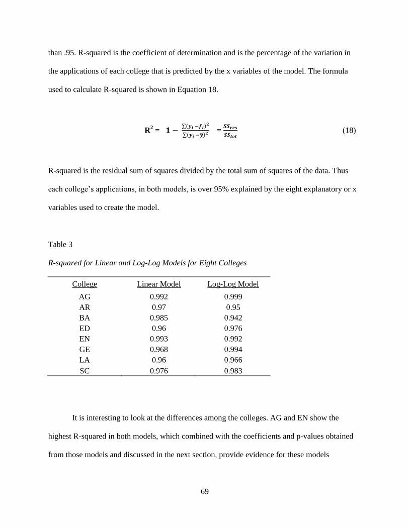
69
than .95. R-squared is the coefficient of determination and is the percentage of the variation in
the applications of each college that is predicted by the x variables of the model. The formula
used to calculate R-squared is shown in Equation 18.
R2 = 𝟏 −
∑(𝒚𝒊 −𝒇𝒊)𝟐
∑(𝒚𝒊 −�̅�)𝟐 =
𝑺𝑺𝒓𝒆𝒔
𝑺𝑺𝒕𝒐𝒕 (18)
R-squared is the residual sum of squares divided by the total sum of squares of the data. Thus
each college’s applications, in both models, is over 95% explained by the eight explanatory or x
variables used to create the model.
Table 3
R-squared for Linear and Log-Log Models for Eight Colleges
College Linear Model Log-Log Model
AG 0.992 0.999
AR 0.97 0.95
BA 0.985 0.942
ED 0.96 0.976
EN 0.993 0.992
GE 0.968 0.994
LA 0.96 0.966
SC 0.976 0.983
It is interesting to look at the differences among the colleges. AG and EN show the
highest R-squared in both models, which combined with the coefficients and p-values obtained
from those models and discussed in the next section, provide evidence for these models

70
effectiveness in predicting applications in these colleges. While the other eight colleges do not
have the same consistently high values, all are very high and justify the model as a predictor.
Statistical significance is used to determine if anything actually happened in a test
or if the coefficients found differ from zero. The null hypothesis, HO, of any test is the
assumption that the coefficient equals zero or nothing happened. The alternative hypothesis, HA,
is the opposite, something in fact did occur or a value is found for the coefficient. The p-value of
a test is the probability of observing an effect if the null is actually true. If the p-value is below a
certain level, there is statistical evidence to reject the null. The level chosen is the significance
level. Another way to describe the significance level is as the probability of rejecting the null if it
is actually true. The lower the significance level, the less likely an event occurs by chance. For
example, a significance level of .10 versus .20 would mean there is less of a chance that an APPS
level predicted by the model happened at random, rather than be caused by variables that are
significant at those levels.
While the model as a whole provides statistically significant predictions, the individual
variables themselves are a different story. With eight colleges and eight variables, there are 64
total variables for the linear and log-log models to analyze. In the linear model, 13 of the 64
show some level of significance (Table 4). With the small sample size of the model, n = 13, it
was decided to test significance levels at .10, .20, and .30 levels. These are indicated in Table 4.

71
Table 4
P-values for Eight Colleges Using Linear Complete Model
College TUI FEES 4YR 2YR INC UN SLR WP
AG 0.034*** 0.041*** 0.154** 0.048*** 0.092*** 0.681 0.794 0.451
AR 0.718 0.973 0.358 0.157** 0.696 0.172** 0.093*** 0.882
BA 0.749 0.704 0.282* 0.313 0.62 0.444 0.55 0.663
ED 0.699 0.984 0.883 0.973 0.662 0.727 0.512 0.652
EN 0.208* 0.257* 0.367 0.482 0.979 0.789 0.624 0.671
GE 0.188** 0.905 0.331 0.479 0.864 0.996 0.224* 0.808
LA 0.974 0.763 0.826 0.991 0.828 0.867 0.553 0.72
SC 0.849 0.963 0.655 0.651 0.303 0.508 0.987 0.553
Note. *p < .30. **p < .20. ***p < .10

72
At the macro level, one of the colleges, AG, provided five of the significant variables,
including three that were significant at the .05 level. Three colleges did not have a single
significant variable at the .30 level, ED, LA, and SC. Tuition was the variable with the most
significant results, three, while wage premium was the only variable that did not have a single
significant value across all eight colleges. Wage premium was retained in the model due to the
high R2 value of the complete model.
Results differed using the log-log model (Table 5). Fourteen of the 64 variables were
significant with seven coming from the AG model. Three colleges were without significant
variables, BA, ED, and LA, while none of the variables had no significant results. The variable
with the most significant values was INC, but two of those were only significant at the .30 level.

73
Table 5
P-values for Eight Colleges Using Log-Log Complete Model
College TUI FEES 4YR 2YR INC UN SLR WP
AG 0.005*** 0.011*** 0.004*** 0.004*** 0.038*** 0.175** 0.627 0.028***
AR 0.751 0.745 0.873 0.464 0.924 0.296* 0.104** 0.902
BA 0.72 0.591 0.379 0.482 0.573 0.465 0.557 0.865
ED 0.652 0.474 0.709 0.432 0.929 0.713 0.624 0.938
EN 0.451 0.337 0.67 0.225 0.839 0.683 0.912 0.274*
GE 0.719 0.802 0.82 0.447 0.23* 0.464 0.146** 0.506
LA 0.578 0.659 0.68 0.934 0.715 0.93 0.521 0.558
SC 0.707 0.876 0.853 0.42 0.276 0.635 0.503 0.715
Note. *p < .30. **p < .20. ***p < .10
74
Agriculture and Life Sciences
The results of the models for the College of Agriculture and Life Sciences are found in
Table 6. The College of Agriculture had the most significant variables in both the linear and log-
log forms. It also had the highest R-squared for both models. The signs on TUI and FEES were
negative as would be expected. Tuition and fees are costs associated with education and would
negatively impact quantity variables such as applications. There were interesting results with
regards to competitors. Four-year competitors had a positive sign, which is indicative of being a
substitute good. That is what was expected for that variable. The three schools used to determine
four-year cost are all major competitors for State U. However, the two-year competitors had a
negative sign. This means that State U and its two-year competitors are actually compliments.
While this does not follow logically, the presence of a large two-year school in the same city as
State U resides in could factor into this relationship. The fact that all the TUI, FEES, 4YR, and
2YR variables were significant for the College of Agriculture means there is statistical evidence
that those four variables affect applications.

75
Table 6
Regression Results for the College of Agriculture and Life Sciences Complete Model
Linear Model Log-Log Model
B SE B
B SE B
Intercept -2424087.26 515829.55
-761.44 56.59
TUI -1.76*** 0.47
-1.64*** 0.22
FEES -1.36*** 0.39
-0.56*** 0.10
4YR 0.89** 0.47
2.99*** 0.37
2YR -12.46*** 3.84
-5.39*** 0.64
INC -0.18*** 0.07
-1.6*** 0.45
UR -63.71 140.47
-0.22** 0.13
SLR -23.47 82.16
-0.04 0.07
WP -2776.30 3208.36
3.45*** 0.86
Year 1220.44*** 258.78 0.41*** 0.03
Note. *p < .30. **p < .20. ***p < .10
The other four variables had several significant variables as well. Income, with a negative
sign, was significant in both models. The formula used to calculate income elasticity (IE) for the
linear model is shown in Equation 19. For the log-log model, the IE is read off as the coefficient
for INC.
IE = 𝝏 𝑸𝒙
𝝏 𝑰∗
𝑰
𝑸𝒙 (19)
The first term is a derivative and is found by taking the coefficient on INC in the linear
regression. The second term is income divided by quantity. Income is normally positive and
quantity is always positive, therefore the second term is normally positive. The first term, the

76
coefficient in the regression, determines the sign of income elasticity. Positive IE is a normal
good, negative is an inferior good, and positive that is greater than one is a luxury good.
The results show that the College of Agriculture is an inferior good for both models. As income
rises, less applications will occur for the College of Agriculture.
While that result may surprise, data collected at State U show that the average starting
salary for Agriculture graduates is one of the bottom three colleges and is only 66% that of the
highest college, Engineering, and much less than Architecture, Business, Geosciences, and
Science (State University, 2016c). As income rises, students matriculate to the higher earning
colleges. Without stratified income data or income data for each individual college, further
conclusions cannot be drawn.
Unemployment rate showed a negative coefficient and was significant in the log-log
model. That is an odd result as theoretically as unemployment rises, college applications rise as
well. The relationship between applications and the student loan rate was not significant in either
model. Wage premium shows a negative coefficient in the linear model, but a positive coefficient
in the log-log model. Wage premium in the linear model is not close to being significant, but in
the log-log model it is significant at the .05 level. The relationship between wage premium and
applications should be positive. The mixed results could be the result of the difficulty in finding
information about wage premiums for most students. They could also result from a non-linear
relationship due to the small sample size of 12 used for the study. A non-linear relationship
would be represented by the log-log model but not by the linear model.

77
Architecture
The College of Architecture results are in Table 7. Five of the variables for Architecture
in both models were significant at one of the three chosen levels. Most of the significant
variables were in the macroeconomic set, with unemployment and the student loan rate being
significant in both linear and log-log models. The signs of the coefficients showed several
unexpected results. In the log-log model, the sign on tuition was positive. If that is correct, it
would mean that as cost rises, applications for Architecture would rise. Also, the income
coefficients in both models were negative, meaning Architecture is an inferior good. These two
results conflict, however as none of those variables were significant, the reason could be lack of
data. Fees and wage premium were not significant in either model.
Table 7
Regression Results for the College of Architecture Complete Model
Linear Model Log-Log Model
B SE B
B SE B
Intercept 147765.53 119416.05
175.48 220.49
TUI -0.04 0.11
0.24 0.70
FEES 0.00 0.10
-0.14 0.39
4YR 0.15 0.14
0.19 1.12
2YR 1.48** 0.79
1.87 2.24
INC -0.01 0.03
-0.20 1.93
UR -82.08** 46.01
-0.67* 0.53
SLR -55.05*** 22.58
-0.54** 0.23
WP 224.12 1391.63
0.49 3.66
Year -73.82 60.10 -0.09 0.12
Note. *p < .30. **p < .20. ***p < .10

78
Two-year and four-year competitors all had positive coefficients, indicating that for
Architecture those competitors are substitutes, which was predicted. Two-year competitor cost
was significant at the .20 level in the linear model. Equation 20 shows the cross-price elasticity
(CPE) formula.
CPE = 𝝏 𝑸𝒙
𝝏 𝑷𝒚∗
𝑷𝒚
𝑸𝒙 (20)
Looking at the second term, price divided by quantity, prices and quantities can never be
negative, therefore the entire second term must always be positive. This means the first half of
the equation, 𝝏 𝑸𝒙
𝝏 𝑷𝒚 , is all that is needed to determine substitutes, those goods with CPE greater
than zero, versus complements, CPE less than zero. Quantity in this case is applications and price
is two-year and four-year competitors. The coefficients of those variables are that first term and
the signs of those coefficients can be used to determine substitutes versus complements. Since
two-year and four-year costs have positive signs, those institutions are substitutes to State U's
College of Architecture.
Business
The College of Business regression results are in Table 8. Only a single variable was
significant for the College of Business and that was only at the .30 level. Even without
significant variables, the signs of the coefficients can be interpreted for patterns.

79
Table 8
Regression Results for the College of Business Complete Model
Linear Model Log-Log Model
B SE B
B SE B
Intercept -67389.47 567272.24
-35.65 180.36
TUI 0.12 0.35
0.14 0.37
FEES -0.19 0.46
-0.22 0.36
4YR -0.93* 0.71
-1.17 1.14
2YR 5.62 4.64
1.78 2.23
INC -0.05 0.10
-0.91 1.44
UR -172.50 196.11
-0.40 0.47
SLR -71.02 105.77
-0.14 0.22
WP -3116.37 6472.95
-0.68 3.68
Year 37.33 283.78 0.03*** 0.09
Note. *p < .30. **p < .20. ***p < .10
The signs for tuition were positive in both models. If these signs are correct, then the
College of Business could have a demand that outpaces supply. However, since the variables are
not significant, more data is needed. Equation 21 is the own-price elasticity (OPE) formula from
the definitions in Chapter One.
ED = 𝝏 𝑸𝒙
𝝏 𝑷𝒙∗
𝑷𝒙
𝑸𝒙 (21)
The second term contains price and quantity. As discussed in the Architecture section, price and
quantity can never be negative, making the second term always positive. The sign of OPE is
found from the derivative term. Quantity for this paper is the applications for each college, while

80
price is the tuition rate. The sign of TUI in each regression gives the sign for OPE for each
college.
One possible explanation for the positive signs on the tuition variable is that demand for
the College of Business is increasing too fast for supply to respond. If demand and supply
increase at the same rate, then the intersections of supply and demand will give a negative slope
for the demand curve when studied with regression. However, what if a college does not have the
space or resources to admit students as fast as they want to come in to the school? The result is a
large increase in demand over time, with a very small supply increase. The supply and demand
intersections would actually slope upward for the time period, giving a regression coefficient that
is positive. Henry Moore, Yale Professor of Economics in the early 1900s, related this idea for
the first time with an example about pig iron (Moore, 1914). 1
The only significant variable was four-year competitor’s costs in the linear model. The
sign on the four-year costs variable was negative. That would indicate that State U’s College of
Business and its four-year competitors were complements. That result is unlikely in rational
consumer’s eyes. Two-year schools were substitutes, which is as predicted. The other variables
were all far from being significant and while some of the signs were interesting, negative signs
on wage premium and unemployment rate, the high p-values make discussion of those values
difficult.
1 A less likely possibility is that of a Veblen Good. A Veblen good has a positive demand curve as well but
for quality reasons. If a person assumes that a good is better because it is more expensive, then the demand for that
good may increase. For example, luxury cars might see their demand actually rise when price reaches a certain point
due to the prestige factor. It is far more likely that college education is a Veblen good rather than a Giffen good.
If the College of Business met these requirements it would lend credence to the idea of the Business
College as a Veblen Good. State U’s College of Business undergraduate program ranks in the top 20 in both
Bloomberg Businessweek and U.S. News & World Report rankings, giving evidentiary support to the superior
product idea (State University, 2016d). In truth, this is supposition since the variables are not significant in these
models. More data is required for confirmation.

81
Education
The regression results for the College of Education are reported in Table 9. No variable
was significant for the College of Education in either model except the trend variable. In fact in
both models, most p-values were well above .5. Statistical interpretations of these results are
unlikely to be beneficial as they show there is no evidence that any of the x variables actually
predict College of Education applications.
Table 9
Regression Results for the College of Education Complete Model
Linear Model Log-Log Model
B SE B
B SE B
Intercept -571802.61 490908.52
-385.46 202.79
TUI -0.39 0.92
0.54 1.09
FEES 0.01 0.50
0.38 0.47
4YR -0.14 0.85
-0.66 1.60
2YR -0.14 3.78
-2.25 2.48
INC -0.05 0.10
0.17 1.79
UR -81.60 212.65
0.23 0.58
SLR -80.50 108.50
-0.15 0.27
WP -3155.37 6323.28
-0.34 4.04
Year 289.38 246.07 0.20* 0.11
Note. *p < .30. **p < .20. ***p < .10
Engineering
The College of Engineering results are in Table 10. The College of Engineering at State
U is ranked in the top 10 among public institutions and top 20 overall for engineering schools
(State University, 2016e). Four variables, two from each model, were significant. Oddly, the two
were different in each model. In the linear model, both TUI and FEES were significant. Even

82
more perplexing, the signs were different for these two cost variables. The sign for tuition was
positive. Similar to the discussion in the College of Business section, this indicates demand may
be adjusting faster than supply.2
Table 10
Regression Results for the College of Engineering Complete Model
Linear Model Log-Log Model
B SE B
B SE B
Intercept -1482533.59 1029353.58
-342.6 114.71
TUI 1.93* 1.21
0.39 0.45
FEES -1.28* 0.92
-0.25 0.22
4YR -1.42 1.34
-0.3 0.64
2YR -6.63 8.29
-2.02* 1.32
INC -0.008 0.27
-0.26 1.18
UR -136.98 468.34
-0.14 0.32
SLR -119.49 219.74
0.016 0.13
WP 6229.32 13267.37
2.84* 2.13
Year 742.71 517.65 0.18* 0.06
Note. *p < .30. **p < .20. ***p < .10
The significant, negative sign on fees is easier to explain. Fees are a cost and as costs rise,
demand drops. However, why would one cost have a positive sign and the other negative? The
best explanation is the relative smooth nature of FEES in the data set. While tuition for the
College of Engineering rose 182.6% from 2003 to 2015, fees only rose 16.4% over the same
period.
2 The College of Engineering might be even more suited to be called a Veblen Good than the College of Business. It
is ranked as highly as the College of Business, but lacks competitors among the major four-year competitor schools
in the state. State U’s College of Engineering is the main campus to secure an Engineering degree in the entire state.
These facts lend credence to the idea of the College of Engineering having a positive sloping demand curve.

83
Both two-year and four-year costs were negative in all models, making those competitors
complements for Engineering. As there is no real alternative for students pursuing engineering
degrees in the state, this makes sense. The macro variables were for the most part highly
insignificant, but the wage premium was significant in the log-log model and showed a positive
sign in both models. A higher-earning degree like engineering would appeal to students when the
premium between high-school degree earners and college-degree earners becomes larger.
Geosciences
The College of Geosciences is the smallest at State U with 159 applicants in 2003 up to
530 in 2013. Geosciences showed four significant variables, with two from each model (Table
11). The student loan rate was significant in both models and had a negative sign. This is an
expected sign for as the loan rate increases, applications would be expected to decrease. Tuition
is significant in the linear model and is negative, which is the expected sign. However, in the log-
log model it turns positive, while being non-significant.

84
Table 11
Regression Results for the College of Geosciences Complete Model
Linear Model Log-Log Model
B SE B
B SE B
Intercept -101072.74 71763.65
-184.62 170.91
TUI -0.17** 0.10
0.31 0.78
FEES -0.007 0.06
0.09 0.33
4YR 0.1 0.09
0.29 1.18
2YR -0.39 0.48
-1.66 1.90
INC 0.0024 0.01
2.11* 1.40
UR -0.14 23.60
0.35 0.41
SLR -19.87* 13.01
-0.41** 0.21
WP 200.86 756.64
2.25 2.98
Year 50.56* 36.07 0.087 0.09
Note. *p < .30. **p < .20. ***p < .10
Income is significant in the log-log model. Using the properties of the log-log model,
where the coefficients are the elasticities without the need for calculation, the coefficient of 2.11
indicates that the College of Geosciences is a normal, luxury good. It is positive, making it a
normal good, and it is greater than 1, which qualifies it as a luxury good. The practical
applications of a geosciences degree, mainly working in the oil and gas sector, could be the cause
of this outcome. The oil and gas sector is cyclical and the time period of this data included a big
upswing in the oil and gas market. The lure of high paying jobs in peak times might cause
students to pick the College of Geosciences during those times and avoid it during lulls. This is
somewhat confirmed by the coefficients on wage premium. In both models they are relatively
large, positive numbers. However, the utility of those numbers is constrained by the lack of
statistical significance.

85
Liberal Arts
The regression results for the College of Liberal Arts are shown in Table 12. Like the
College of Education, there are no significant variables in either model and none have a p-value
lower than .5. Statistical interpretations of these results are unlikely to be beneficial as they
show there is no evidence that any of the x variables actually cause College of Liberal Arts
applications.
Table 12
Regression Results for the College of Liberal Arts Complete Model
Linear Model Log-Log Model
B SE B
B SE B
Intercept -220482.81 519761.24
-55.11 142.77
TUI 0.03 0.75
0.41 0.66
FEES -0.14 0.42
-0.14 0.28
4YR -0.16 0.65
-0.46 1.00
2YR -0.04 3.53
-0.14 1.60
INC 0.02 0.09
0.47 1.18
UR -31.18 171.56
-0.03 0.35
SLR -63.34 95.20
-0.13 0.18
WP 2165.27 5499.45
1.65 2.52
Year 110.18 261.19 0.03 0.08
Note. *p < .30. **p < .20. ***p < .10
Sciences
The final college is Sciences (Table 13). Only one variable was significant for sciences,
income in the log-log model, but income in the linear model was very nearly a second. In both
instances the sign on income was positive, which is expected. Using the log-log model, the
income elasticity can be determined as 1.94. That would place the College of Sciences in the

86
same category as Geosciences, as a normal, luxury good. Many scholars would claim that all
higher education would be normal, luxury goods, so this result is not unexpected. What is
unexpected is that only two of the eight colleges showed this result.
Table 13
Regression Results for the College of Sciences Complete Model
Linear Model Log-Log Model
B SE B
B SE B
Intercept 639364.59 837458.67
225.54 177.98
TUI -0.25 1.19
0.33 0.81
FEES -0.03 0.66
-0.06 0.34
4YR 0.51 1.03
-0.25 1.23
2YR 2.82 5.63
1.85 1.98
INC 0.18 0.15
1.94* 1.46
UR 206.39 275.48
0.23 0.43
SLR 2.65 151.94
-0.17 0.22
WP 5883.67 8831.43
1.25 3.11
Year -326.31 420.90 -.13* 0.09
Note. *p < .30. **p < .20. ***p < .10
Conclusion
The complete model demonstrated very high R-squared values, indicating its fitness for
prediction, and had several significant variables at key, expected locations. There were numerous
anomalies including why the College of Agriculture and Life Sciences had a high percentage of
significant variables and the propensity of the colleges to be inferior goods. These factors limit
the use of the complete forecast model as a policy tool. A reduced model was determined using
directed graph principles in order to assist policymakers and lawmakers to a greater extent.

87
Policy Model
The complete model was reduced to a policy model through the Directed Graph
procedure. Correlation matrices were collected for each college. These matrices are presented in
Appendix B. The matrices were fed into the TETRAD II program and that program removed
edges that did not have statistically significant correlations and partial correlations at the .20
level. The results of the TETRAD II are shown in Table 14.
The TETRAD results show that several variables have little or no causal influence on
applications. For TETRAD purposes applications was X1. FEES, INC, UN, and SLR had no
statistically significant correlations with applications. Therefore, the decision was made to
remove those four variables from the policy model. Wage premium (X9) was an indicator of
applications for one of the eight colleges, Sciences. It was decided to remove wage premium
from the policy model despite this result. The lack of confidence in the wage premium variable
was the deciding factor. Without differing premiums for each college, there is a lack of data that
relates at the college level. The presence of a directed edge gives credence to the idea that wage
premium does affect application decisions, but more data is needed.
The TETRAD results leave TUI, 4YR, and 2YR as the only variables in the policy
model. Even though all three variables were not given edges for every college, all were left in the
policy model for each college. Each of those three showed some relationship between themselves
and applications. Both TUI and 2YR showed a directed edge on at least one college. That is
enough evidence for inclusion if taken with the lack of observations in the data. The directed
acyclic graphs for each of the eight colleges are shown in Appendix C.

88
Table 14
TETRAD II Results for Eight Colleges
.20 SL AG AR ED EN GE LA BA SC
X2 (TUI) -- X4 -- X4 →X1 -- X4 →X4 -- X4 →X4
X3 (FEES)
X4 (4YR) -- X5 -- X5 -- X5 -- X5 -- X5 →X5
X5 (2YR) →X1 →X1 →X1 →X1 ; → X4 →X1 ; → X4 →X1 ; → X4
X6 (INC)
X7 (UN) ** ** ** ** ** ** ** **
X8 (SLR)
X9 (WP) →X1
Notes.** X7 -- X8, X7 -- X9

89
As shown above, directed graph analysis led to the reduction of the model to three x
variables, tuition (TUI), four-year competitors (4YR), and two-year competitors (2YR).
Regressions were then run with those three x variables and the eight college’s applications as the
dependent variable. R-squared values obtained from the regressions are shown in Table 15. As
with the complete model, R-squared values are high. However, R-squared values cannot be
compared across models of different sizes. R-squared will automatically increase in value with
the inclusion of any variable, significant or random. Simply increasing the size of the model will
make R-squared increase and make a model look like a better predictor.
Table 15
R-squared Results for Policy Model
College Linear Model Log-Log Model
AG 0.922 0.983
AR 0.878 0.854
BA 0.924 0.916
ED 0.942 0.962
EN 0.97 0.986
GE 0.982 0.968
LA 0.959 0.949
SC 0.948 0.964
Comparing two models that have different sizes, different numbers of x variables,
requires comparing the Adjusted R-squared. Table 16 shows the Adjusted R-squared values for
both linear and log-log and both the complete and policy models. The comparisons need to be
made between the complete and policy model for each of the linear and log-log format. Values
that are bolded were higher for that particular model. For the majority of the colleges, the policy

90
model had a higher adjusted R-squared, meaning the policy model is better for analysis. For the
AG, AR, and GE colleges, the complete model was better in at least one form. For this reason,
elasticity calculations will include the complete and policy models for those three colleges. For
the other five, only the policy model is included in elasticity calculations.
Table 16
Adjusted R-squared Values for Complete and Policy Models
Complete Model Policy Model
College Linear Model L-L Model
Linear Model L-L Model
AG 0.967* 0.997*
0.883 0.974
AR 0.88* 0.802*
0.817 0.781
BA 0.84 0.768
0.885* 0.873*
ED 0.84 0.903
0.913* 0.942*
EN 0.939 0.966
0.955* 0.979*
GE 0.972 0.975*
0.973* 0.953
LA 0.871 0.862
0.939* 0.924*
SC 0.903 0.931
0.922* 0.945*
Notes. *Higher Adjusted R2
In both the linear and log-log models for the reduced, policy model, there were a much greater
percentage of significant variables. In the linear model, 12 variables out of 24 were significant
(Table 17). The log-log model had 10 out of 24 significant (Table 18). That means 46% of the
variables were significant in the reduced model, while only 21% (27 out of 128) were significant

91
in the complete model. All three variables were significant for multiple colleges. Only one
college lacked a significant variable in either model, Liberal Arts, and Education did not have
one in the log-log model.
Table 17
P-values for Linear Policy Model
College TUI 4YR 2YR
AG 0.159** 0.369 0.39
AR 0.725 0.402 0.244*
BA 0.715 0.018*** 0.92
ED 0.613 0.185** 0.796
EN 0.033*** 0.006*** 0.2**
GE 0.005*** 0.259* 0.872
LA 0.325 0.548 0.988
SC 0.129** 0.11** 0.22**
Note. *p < .30. **p < .20. ***p < .10
Table 18
P-values for Log-log Policy Model
College TUI 4YR 2YR
AG 0.006*** 0.13** 0.031***
AR 0.772 0.646 0.545
BA 0.733 0.091*** 0.966
ED 0.646 0.846 0.592
EN 0.243* 0.204* 0.02***
GE 0.102** 0.578 0.464
LA 0.845 0.587 0.592
SC 0.287* 0.728 0.03***
Note. *p < .30. **p < .20. ***p < .10

92
Agriculture and Life Sciences
The results of the regression run on the policy model for the College of Agriculture and
Life Sciences are shown in Table 19. Tuition was significant in both the linear and log-log
models and had the expected negative sign in both. Four-year and two-year competitors were
significant in the log-log model. In that model, four-year schools had a positive value, meaning
they are substitutes. Two-year schools had a negative value, indicating complements. Both ideas
make sense relative to the conditions of State U. The College of Agriculture is large at State U,
but there are other colleges in the state that provide competition. The college has over thirty
degree programs which also increase the amount of potential substitutes.
Table 19
Regression Results for College of Agriculture Policy Model
Linear Model Log-Log Model
B SE B
B SE B
Intercept -1237465.78 497792.57
-560.40 96.61
TUI -0.98** 0.63
-1.6*** 0.43
4YR -0.56 0.59
1.44** 0.85
2YR -3.47 3.82
-3.0031*** 1.15
Year 620.89** 249.96 0.29*** 0.05
Note. *p < .30. **p < .20. ***p < .10
Two-year schools would generally be considered substitutes for State U as well.
However, the presence of a large, reputable two-year college in the same town as State U makes
it possible to justify the results as complements. Many students attend the two-year college for
one to four semesters because it is cheaper than State U and they can still enjoy the atmosphere
that goes along with being a part of State U. The university also has partnership agreements with

93
the local junior college in order to allow some students not initially accepted into State U the
opportunity to apply at a later date. The behavior pattern of the two schools indicates a
complementary role in higher education between the two; a pattern that is backed up by the data
for the College of Agriculture.
Elasticity calculations for own-price elasticity (OPE), cross-price elasticity between State
U and four-year competitors (CPE4), and cross-price elasticity between State U and two-year
colleges (CPE2) were made in several ways. The log-log model allows elasticity to be calculated
as the estimated percent change in the dependent variable for a percent change in the
independent variable. This measure is the elasticity over the entire time period of the data set.
The College of Agriculture had a higher adjusted R-square value for the complete model,
therefore elasticity was found for both the complete and policy model (Table 20).
Table 20
Log-log Form Elasticities for College of Agriculture Models
OPE CPE4 CPE2
Complete -1.637 2.99 -5.387
Policy -1.600 1.44 -3.003
Since most OPE are negative, taking the absolute value allows interpretation. Recall from
the definitions in Chapter One, if the absolute value is greater than 1 that is called an elastic
good. If the absolute value is less than 1, it is an inelastic good. If the elasticity has an absolute
value of greater than 1, then the numerator of the equation is greater than the denominator. OPE
is percent change in quantity of percent change in price. If that value is greater than 1, then if

94
price increases by 1%, quantity must decrease by greater than 1%, decreasing revenue. In order
to increase revenue, price must drop. The opposite is true for an inelastic good.
OPE for the complete model was -1.637, making it an elastic good and meaning a 1%
increase in the cost of tuition for the College of Agriculture would result in a 1.637% decrease in
the number of applications. The policy model gives the OPE as -1.6, making it an inelastic good
and resulting in a 1% increase in the cost of tuition causing a 1.6% drop in applications. The two
models give similar results, calling the College of Agriculture an elastic good. Thus lowering
tuition would generate more applications and more revenue.
The elasticities can also be calculated for the linear model. There is a difference. These
elasticities can be calculated for each year. They must be calculated using the OPE formula given
in Equation 22
OPE = 𝝏 𝑸𝒙
𝝏 𝑷𝒙∗
𝑷𝒙
𝑸𝒙 (22)
The coefficients, the first term, will be the same for every year, while the tuition cost and
applications change every year. The results for the complete model and policy model are shown
in Tables 21 and 22, respectively. They provide more clarity. Every OPE in the complete model
has an absolute value greater than 1. They are all elastic. The policy model shows similar results,
all years but one are elastic. Again, this indicates that the College of Agriculture is an elastic
good and to lower costs would increase applications and increase revenue.

95
Table 21
Elasticities for College of Agriculture Linear Complete Model
Year OPE CPE4 CPE2
2003 -2.683 2.457 -9.498
2004 -3.508 3.048 -10.14
2005 -3.792 2.992 -10.392
2006 -4.451 3.743 -12.41
2007 -3.829 3.137 -10.471
2008 -3.671 2.978 -10.124
2009 -3.52 2.883 -9.877
2010 -3.31 2.787 -9.605
2011 -2.618 2.332 -8.479
2012 -2.674 2.451 -9.155
2013 -1.73 1.653 -5.971
2014 -2.236 1.798 -6.562
2015 -2.101 1.666 -6.221

96
Table 22
Elasticities for College of Agriculture Linear Policy Model
Year OPE CPE4 CPE2
2003 -1.471 -1.527 -2.59
2004 -1.942 -1.913 -2.792
2005 -2.251 -2.014 -3.068
2006 -2.205 -2.102 -3.058
2007 -2.266 -2.105 -3.081
2008 -2.077 -1.91 -2.849
2009 -2.021 -1.877 -2.821
2010 -1.86 -1.775 -2.684
2011 -1.544 -1.56 -2.488
2012 -1.465 -1.522 -2.494
2013 -0.975 -1.056 -1.673
2014 -1.193 -1.088 -1.741
2015 -1.202 -1.081 -1.771
Tables 21 and 22 also show how the OPE changes over time. Both spike in the 2005-
2007 range and start to drop. Perhaps this is a result of the increase in tuition in some of the other
colleges at State U. If the College of Engineering increases tuition, Agriculture has become
relatively cheaper, pushing OPE closer to 1. That time period also corresponds to the last large
increase in farm commodity prices. Higher prices certainly could have increased demand for jobs
in the agriculture sector, boosting demand for the degree.
The two models differ in regards to their CPE4 valuations. The complete model has
positive values, substitutes, in both the linear and log-log formats, while the policy model has
negative values, complements. As the complete model does have a higher Adjusted R-squared

97
and the 4YR variable is significant in both the complete model formats, evidence is greater that
the College of Agriculture is substitutes with its four-year competition.
The models have similar results for CPE2, only differing in magnitude. All four models
place the College of Agriculture and the two-year colleges as complements. Anecdotal evidence
suggests that the College of Agriculture has a higher percentage of transfer students than the
other State U Colleges. This would lead to a complementary relationship for the two entities.
Architecture
The results of the policy model regression for the College of Architecture are in Table 23.
Contrary to the results in the complete model, only a single variable, linear model 2YR, is
significant. This limits the impact of the policy model in this case.
Table 23
Regression Results for College of Architecture Policy Model
Linear Model Log-Log Model
B SE B
B SE B
Intercept -6658.63 71.14
-44.22 143.23
TUI -0.03 0.21
-0.15 0.50
4YR -0.09 0.56
-0.43 0.90
2YR 0.82* 0.81
0.93 1.47
Year 3.42 0.04 0.02 0.08
Note. *p < .30. **p < .20. ***p < .10
As with Agriculture the complete model gave higher Adjusted R-squared values and had
more significant variables. Therefore, elasticity calculations were obtained for both the complete
and policy models. The calculation for the log-log forms is given in Table 24.

98
Table 24
Log-log Form Elasticities for College of Architecture Models
OPE CPE4 CPE2
Complete 0.244 0.194 1.87
Policy -0.149 -0.429 0.931
The policy value for OPE has Architecture as an inelastic good. The complete model log-
log form actually shows Architecture with a positive OPE. As tuition costs rise, applications rise
as well. Calculated values for the linear complete model in Table 25 give similar results to the
policy model in both log-log and linear. All values are between -.12 and -.22. The very consistent
results help place Architecture as an inelastic product. If State U were to raise tuition prices in
the College of Architecture, applications would fall a small amount, but revenue would rise a
much larger percentage.
In both the log-log and linear models, CPE4 and CPE2 are positive for the complete
model. Both four-year and two-year schools act as substitutes for the College of Architecture.
This is consistent with the predictions made in Chapter Three. It is also consistent with the idea
of competition between higher education entities and the lack of prestige and recognition of State
U's College of Architecture.
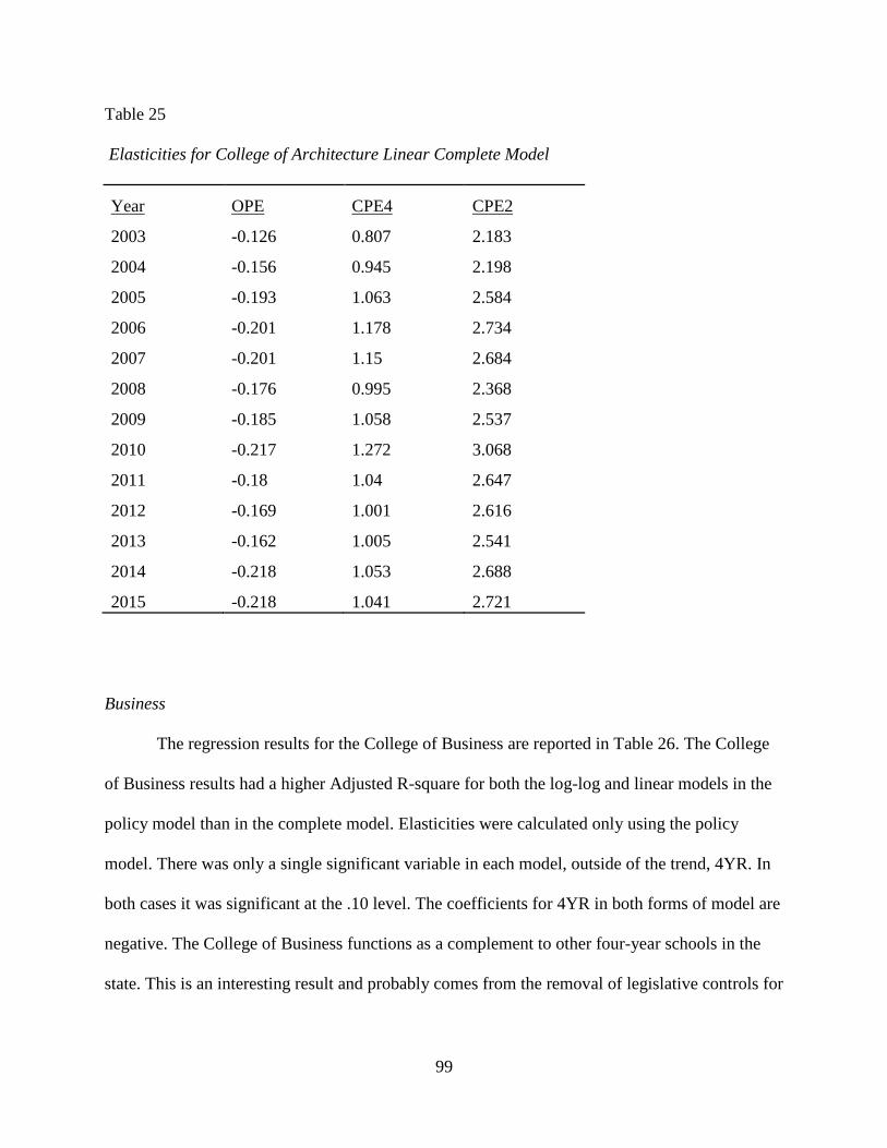
99
Table 25
Elasticities for College of Architecture Linear Complete Model
Year OPE CPE4 CPE2
2003 -0.126 0.807 2.183
2004 -0.156 0.945 2.198
2005 -0.193 1.063 2.584
2006 -0.201 1.178 2.734
2007 -0.201 1.15 2.684
2008 -0.176 0.995 2.368
2009 -0.185 1.058 2.537
2010 -0.217 1.272 3.068
2011 -0.18 1.04 2.647
2012 -0.169 1.001 2.616
2013 -0.162 1.005 2.541
2014 -0.218 1.053 2.688
2015 -0.218 1.041 2.721
Business
The regression results for the College of Business are reported in Table 26. The College
of Business results had a higher Adjusted R-square for both the log-log and linear models in the
policy model than in the complete model. Elasticities were calculated only using the policy
model. There was only a single significant variable in each model, outside of the trend, 4YR. In
both cases it was significant at the .10 level. The coefficients for 4YR in both forms of model are
negative. The College of Business functions as a complement to other four-year schools in the
state. This is an interesting result and probably comes from the removal of legislative controls for

100
tuition in 2004-2005. All four-year schools were allowed to set their tuition rates and the
numbers have dramatically increased for all.
Table 26
Regression Results for College of Business Policy Model
Linear Model Log-Log Model
B SE B
B SE B
Intercept -726861.71 283036.61
-175.77 71.14
TUI -0.09 0.24
0.07 0.21
4YR -1.19*** 0.40
-1.08*** 0.56
2YR 0.24 2.26
-0.035 0.81
Year 365.59*** 142.09 0.1*** 0.04
Note. *p < .30. **p < .20. ***p < .10
For both models, TUI and 2YR were far from significant. Given the limits of the data set,
there is hesitation to draw conclusions from those two variables. In the case of both tuition and
two-year competitors, the signs switch from one model to the next. This indicates that either the
true value is close to zero for each or there is not enough data to determine the true relationship.
In the case of tuition, if the value is close to zero, that provides insight. A very small coefficient
in the log-log model means a highly inelastic product. This is confirmed by looking at Table 27
which has the linear elasticity calculations. The OPE calculations are all between -.05 and -.12.
While there is not enough statistical evidence to say for certain that the College of Business is an
inelastic good, that conclusion is somewhat supported by the evidence. The College of Business
has led the way in differential tuition at State U and it will require more data to confirm that this
was the proper policy.

101
Table 27
Elasticities for College of Business Linear Policy Model
Year OPE CPE4 CPE2
2003 -0.054 -1.293 0.07
2004 -0.076 -1.725 0.081
2005 -0.073 -1.506 0.074
2006 -0.09 -1.975 0.092
2007 -0.096 -2.058 0.097
2008 -0.108 -1.835 0.088
2009 -0.108 -1.883 0.091
2010 -0.119 -2.136 0.104
2011 -0.101 -2.039 0.104
2012 -0.09 -1.88 0.099
2013 -0.088 -1.9 0.097
2014 -0.097 -1.87 0.096
2015 -0.085 -1.627 0.086
Education
In the complete model, the College of Education was one of the colleges that had no
significant variables. While the policy model for Education does not have many significant
variables, the 4YR variable is significant in the linear model and the trend variable is significant.
All coefficient values for Education are negative (Table 28). The signs on TUI would agree with
economic theory. However, those on 4YR and 2YR relate that the College of Education would
be complements with its four-year and two-year competitors. Under ordinary circumstances, that
would seem illogical. As with several other colleges, it could be argued that two-year schools are
complements to State U due to the proximity of a junior college and the partnerships that exist
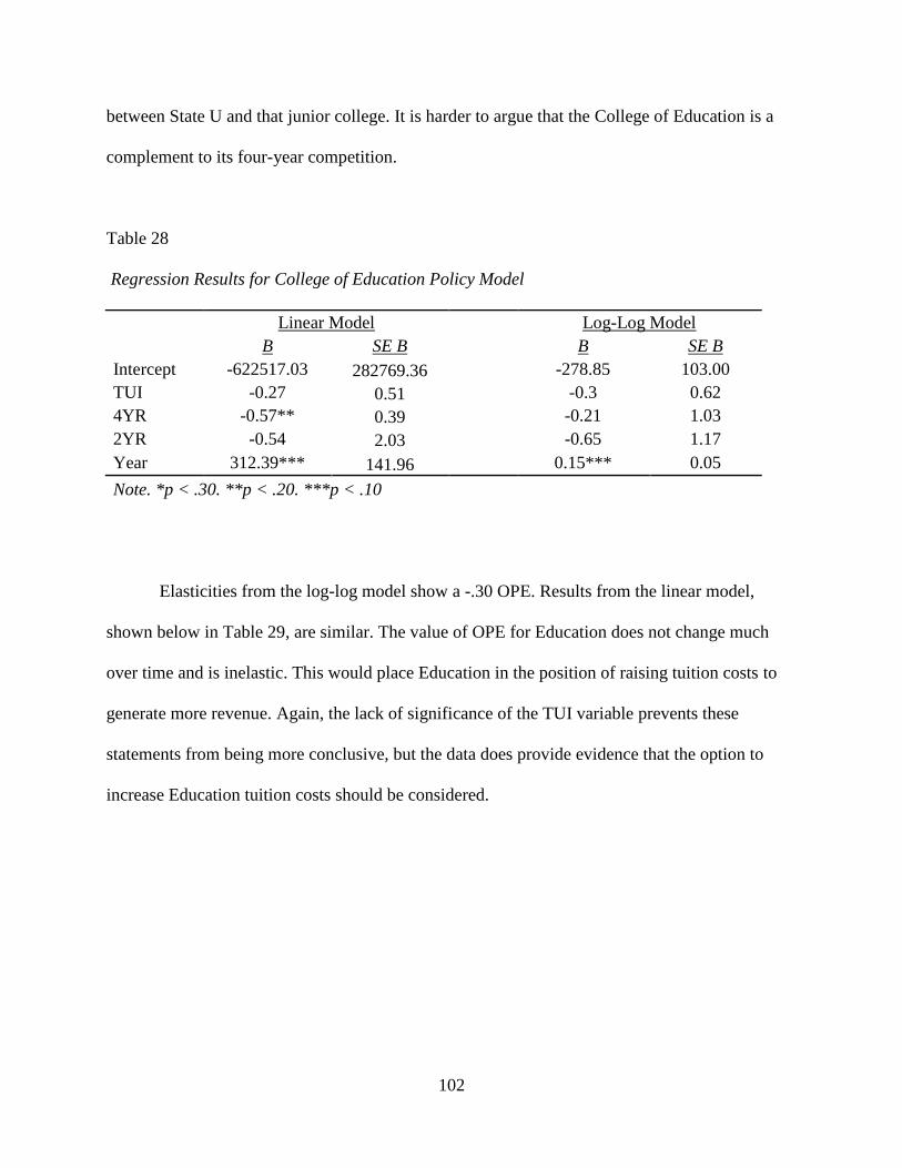
102
between State U and that junior college. It is harder to argue that the College of Education is a
complement to its four-year competition.
Table 28
Regression Results for College of Education Policy Model
Linear Model Log-Log Model
B SE B
B SE B
Intercept -622517.03 282769.36
-278.85 103.00
TUI -0.27 0.51
-0.3 0.62
4YR -0.57** 0.39
-0.21 1.03
2YR -0.54 2.03
-0.65 1.17
Year 312.39*** 141.96 0.15*** 0.05
Note. *p < .30. **p < .20. ***p < .10
Elasticities from the log-log model show a -.30 OPE. Results from the linear model,
shown below in Table 29, are similar. The value of OPE for Education does not change much
over time and is inelastic. This would place Education in the position of raising tuition costs to
generate more revenue. Again, the lack of significance of the TUI variable prevents these
statements from being more conclusive, but the data does provide evidence that the option to
increase Education tuition costs should be considered.

103
Table 29
Elasticities for College of Education Linear Policy Model
Year OPE CPE4 CPE2
2003 -0.38 -1.466 -0.385
2004 -0.483 -1.768 -0.4
2005 -0.464 -1.543 -0.365
2006 -0.553 -1.961 -0.442
2007 -0.544 -1.878 -0.426
2008 -0.544 -1.859 -0.43
2009 -0.478 -1.65 -0.384
2010 -0.48 -1.705 -0.399
2011 -0.403 -1.515 -0.375
2012 -0.476 -1.653 -0.42
2013 -0.364 -1.318 -0.324
2014 -0.401 -1.315 -0.326
2015 -0.359 -1.191 -0.302
Engineering
In the complete model studied earlier, the College of Engineering at State U had four
significant variables, but all were only significant at the .30 level. Engineering is the college that
gains the most from switching to the policy model. All six variables are now significant at one of
the three levels (Table 30). Every coefficient can be interpreted with confidence as there is
statistical evidence that those coefficients are different than zero and that the sign if correct. The
TUI coefficient is positive for both the linear and log-log models. As discussed in the complete
model section on the College of Business, a positive coefficient on TUI would be a sign of a that
demand is changing faster than supply. This could result in a positive sloped demand curve,

104
meaning as costs rise, demand also rises. The complete model also had Engineering with a
positive demand over the time period of this data set, thus the policy model is more evidence that
Moore’s problem many exist here (Moore, 1914).
Table 30
Regression Results for College of Engineering Policy Model
Linear Model Log-Log Model
B SE B
B SE B
Intercept -1933883.72 600456.75
-325.58 56.16
TUI 1.61*** 0.62
0.3* 0.24
4YR -2.61*** 0.69
-0.51* 0.37
2YR -5.41** 3.87
-1.62*** 0.56
Year 971.29*** 301.42 0.17*** 0.03
Note. *p < .30. **p < .20. ***p < .10
OPE can be found by looking at the coefficient on TUI in the log-log model, which is .30.
Table 31 has the linear model elasticities, which show an OPE of .61 to .93. To increase revenue
for a Engineering, price or in this case cost can be increased. The College of Engineering at State
U is a prime candidate for increased differential tuition. The data says that increasing tuition
would generate more revenue, but would not have the side effect inherent in inelastic goods of
decreasing applications.
The 4YR and 2YR coefficients for both models are negative. Engineering and its four-
year competitors are complements, as are Engineering and its two-year competitors. While this
seems counterintuitive, the circumstances surrounding the College of Engineering at State U
support the argument. State U has the only major College of Engineering in the state and thus
attracts most of the in-state students interesting in Engineering. The College is also well

105
renowned world-wide and attracts out-of-state and international students in great numbers. Many
students use the local junior college as an entry point, taking core curriculum classes prior to
transferring to the College of Engineering. The argument that these schools are complements to
the College of Engineering is strong and is backed up by the data.
Table 31
Elasticities for College of Engineering Linear Policy Model
Year OPE CPE4 CPE2
2003 0.608 -1.791 -1.02
2004 0.83 -2.319 -1.136
2005 0.848 -2.151 -1.101
2006 0.808 -2.182 -1.066
2007 0.895 -2.357 -1.159
2008 0.827 -2.155 -1.079
2009 0.839 -2.21 -1.115
2010 0.824 -2.23 -1.132
2011 0.93 -2.312 -1.239
2012 0.87 -2.227 -1.226
2013 0.748 -1.996 -1.062
2014 0.746 -1.63 -0.876
2015 0.737 -1.591 -0.875
Geosciences
The regression results for the College of Geosciences are shown in Table 32. Geosciences
were the one college that was split on whether the complete or policy model was better. The
Adjusted R-squared was higher for the log-log model in the complete form of the model, but

106
higher for the linear model in the policy form. In both types of model for the policy, TUI was
significant and had a negative sign. This is an expected sign, having a downward sloping demand
curve.
Table 32
Regression Results for College of Geosciences Policy Model
Linear Model Log-Log Model
B SE B
B SE B
Intercept -105544.46 44843.49
-128.36 133.25
TUI -0.27*** 0.07
-1.28** 0.69
4YR 0.079* 0.06
0.78 1.35
2YR -0.061 0.37
1.27 1.65
Year 52.89*** 22.52 0.064 0.07
Note. *p < .30. **p < .20. ***p < .10
Table 33
Log-log Form Elasticities for College of Geosciences Models
OPE CPE4 CPE2
Complete 0.306 0.292 -1.66
Policy -1.28 0.783 1.267
The OPE for Geosciences is problematic. The complete model was the better model to
use when looking at the log-log design and the OPE is the coefficient which was .31 (Table 33).
This would seem to suggest that Geosciences has a positive demand, like Engineering and
Business. However, Table 34 gives the elasticity calculations for the linear, policy model and all
the OPE are negative. In fact the absolute value of each is greater than 1, which indicates an

107
elastic good. These results are diametrically opposed. One says to raise price, Giffen, while the
other says to lower price, elastic. The only statistical support is the fact that while the log-log
model Adjusted R-squared was higher in the complete versus policy model, the variable TUI in
the complete model was not significant. If that evidence is considered, then the -1.28 elasticity
from the log-log policy model may be a truer indicator of the elasticity of Geosciences.
However, more data is necessary in order to confirm this hypothesis.
Table 34
Elasticities for College of Geosciences Linear Policy Model
Year OPE CPE4 CPE2
2003 -2.329 1.239 -0.265
2004 -2.866 1.447 -0.266
2005 -3.187 1.461 -0.281
2006 -3.642 1.779 -0.326
2007 -3.339 1.589 -0.293
2008 -2.869 1.352 -0.254
2009 -2.359 1.122 -0.213
2010 -2.134 1.044 -0.199
2011 -1.781 0.922 -0.185
2012 -1.633 0.87 -0.18
2013 -1.341 0.744 -0.149
2014 -1.768 0.857 -0.173
2015 -1.775 0.848 -0.175
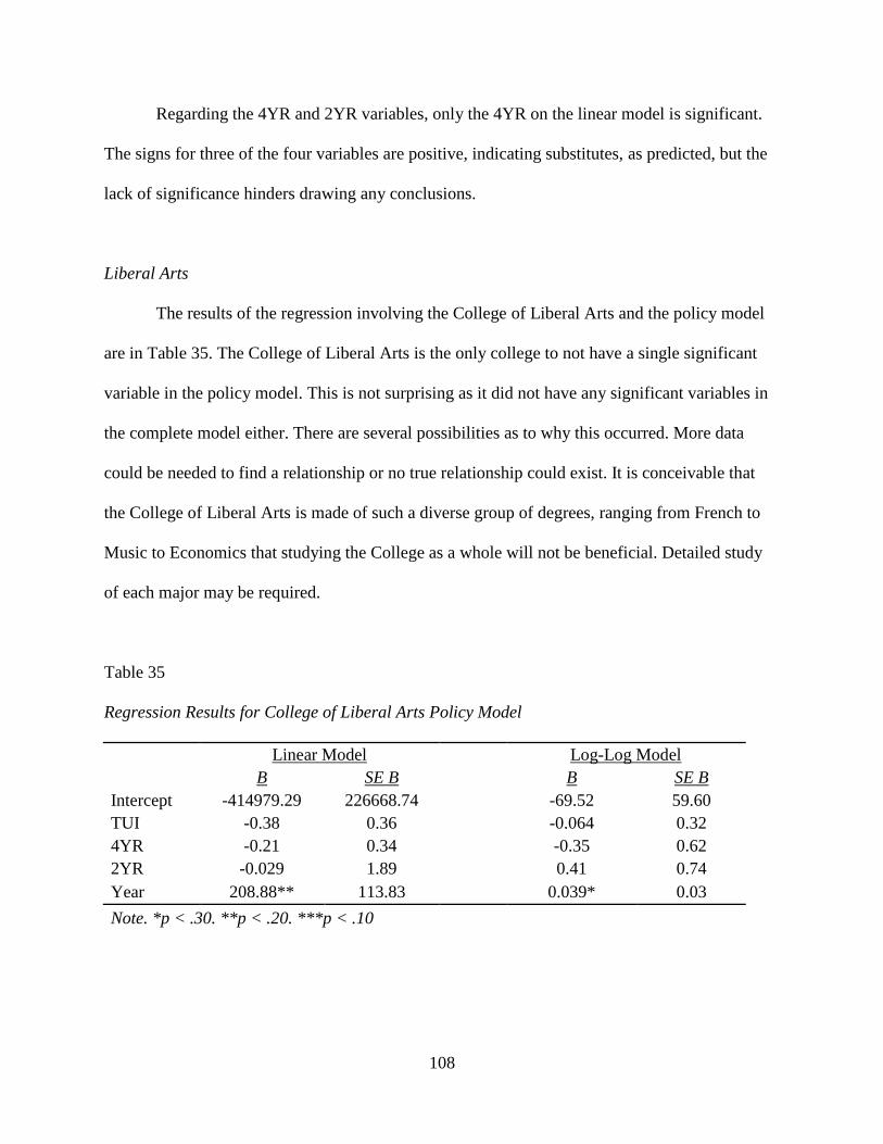
108
Regarding the 4YR and 2YR variables, only the 4YR on the linear model is significant.
The signs for three of the four variables are positive, indicating substitutes, as predicted, but the
lack of significance hinders drawing any conclusions.
Liberal Arts
The results of the regression involving the College of Liberal Arts and the policy model
are in Table 35. The College of Liberal Arts is the only college to not have a single significant
variable in the policy model. This is not surprising as it did not have any significant variables in
the complete model either. There are several possibilities as to why this occurred. More data
could be needed to find a relationship or no true relationship could exist. It is conceivable that
the College of Liberal Arts is made of such a diverse group of degrees, ranging from French to
Music to Economics that studying the College as a whole will not be beneficial. Detailed study
of each major may be required.
Table 35
Regression Results for College of Liberal Arts Policy Model
Linear Model Log-Log Model
B SE B
B SE B
Intercept -414979.29 226668.74
-69.52 59.60
TUI -0.38 0.36
-0.064 0.32
4YR -0.21 0.34
-0.35 0.62
2YR -0.029 1.89
0.41 0.74
Year 208.88** 113.83 0.039* 0.03
Note. *p < .30. **p < .20. ***p < .10

109
Table 36
Elasticities for College of Liberal Arts Linear Policy Model
Year OPE CPE4 CPE2
2003 -0.231 -0.235 -0.009
2004 -0.306 -0.295 -0.01
2005 -0.31 -0.271 -0.009
2006 -0.353 -0.329 -0.011
2007 -0.38 -0.345 -0.011
2008 -0.351 -0.315 -0.01
2009 -0.337 -0.306 -0.01
2010 -0.351 -0.328 -0.011
2011 -0.331 -0.327 -0.012
2012 -0.314 -0.319 -0.012
2013 -0.289 -0.306 -0.011
2014 -0.349 -0.325 -0.012
2015 -0.335 -0.307 -0.011
The elasticity calculations for the College of Liberal Arts are shown in Table 36.
Sciences
The results for the College of Sciences are shown in Table 37. Like Engineering,
Sciences shows the great improvement in moving from the complete to the policy model.
Whereas in the complete model, there was only one significant variable for Sciences, there are
now five. TUI is significant and negative for both linear and log-log forms. Again, this is
consistent with economic theory and will provide negative OPE as expected. In the log-log
model, the OPE is decidedly inelastic, -.53. However, when looking at the linear model and the
elasticity over time, the College of Sciences' OPE varies from -.75 to -1.25 (Table 38). More

110
recent calculations show Sciences very close to -1 or a unit elastic interpretation. A value of OPE
close to -1 is ideal and it appears that the College of Sciences is operating at that level. Looking
at the log-log only, one might say costs can be raised with no issues. However with the split
decision, a small tuition increase is acceptable. That would also generate more evidence to adjust
the tuition in the future.
Table 37
Regression Results for College of Sciences Policy Model
Linear Model Log-Log Model
B SE B
B SE B
Intercept 456779.19 477871.12
177.15 88.78
TUI -1.26** 0.74
-0.53* 0.46
4YR 1.25** 0.69
0.32 0.90
2YR 5.24* 3.93
2.88*** 1.10
Year -229.57 239.97 -0.093*** 0.05
Note. *p < .30. **p < .20. ***p < .10
The coefficients for 4YR and 2YR are all positive with three being significant. This is
solid evidence that four-year and two-year colleges are substitutes for the College of Sciences.
Every one of State U’s major competitors has a College of Sciences or teaches science courses,
so it stands to reason that these institutions would function as substitutes.

111
Table 38
Elasticities for College of Sciences Linear Policy Model
Year OPE CPE4 CPE2
2003 -0.888 1.593 1.842
2004 -1.104 1.88 1.87
2005 -1.172 1.812 1.883
2006 -1.252 2.063 2.047
2007 -1.202 1.93 1.926
2008 -1.108 1.761 1.791
2009 -1.012 1.624 1.665
2010 -0.981 1.618 1.668
2011 -0.854 1.49 1.621
2012 -0.754 1.354 1.513
2013 -0.771 1.443 1.559
2014 -1.071 1.753 1.913
2015 -1.077 1.738 1.941
Conclusion
The policy model resulted in a higher percentage of significant variables. It was also a
better model, based on R-squared, in a majority of the colleges than was the complete model.
This allowed more precise elasticity calculations to be made. For the eight colleges, there was
statistical evidence to find two to be elastic, Agriculture and Geosciences. Taken solely as an
economic question, those two colleges would benefit from lowering tuition costs. They would
see an uptick in applications and likely enrollments, while also increasing their revenue.
Statistical evidence was found to state Engineering has a positive demand. While this is
unlikely to be true over the long term, it is likely to be at least very inelastic. Engineering would

112
benefit from an increase in tuition. Revenues would rise and if it is truly has a positive demand,
applications would rise as well. If it proves to be inelastic, applications would fall as revenue
increases, but at a much smaller percentage.
The College of Sciences has statistical support to being a unit elastic good. Its OPE in
years 2014-15 was calculated as close to -1 and all observations were within 25% of -1. The
evidence leads to the idea that Sciences is priced correctly. Elasticity should of course be
monitored, but tuition should not be changed drastically.
Three colleges, Architecture, Business, and Education, were found to be inelastic, but did
not have significant variables for tuition. However, in each case, there was some evidence that
suggests the inelastic classification is correct. All three colleges stand to benefit from increasing
tuition. Revenues would increase and while applications and enrollments would drop, the
percentage drop would be less than the percentage increase in tuition. Without statistical
significance a stronger statement cannot be made, but it seems likely that those three colleges are
inelastic.
The last college, Liberal Arts, is extremely hard to read. The elasticities calculated
suggest it is inelastic, but none of the variables are significant and there is no additional
information that leads to that opinion. Suggesting raising tuition would be a simple guess in the
case of Liberal Arts and conclusions need to wait on more information.

113
CHAPTER V
IMPLICATIONS AND CONCLUSIONS
The implications section provides a summary of the results, including answers to the
paper’s nine research questions. A conclusion follows stating the implications of the study both
from an economic and access perspective. Limitations and future research end the chapter.
Summary
Two types of models were created. The first was the complete model with all eight
variables included, while the second used Directed Graphs to remove variables that did not have
statistically significant correlations. Both linear and log-log functional forms were used in both
cases.
In the complete model, both functional forms showed high R-squared values for all eight
of the colleges: Agriculture (AG), Architecture (AR), Business (BA), Education (ED),
Engineering (EN), Geosciences (GE), Liberal Arts (LA), and Sciences (SC). High R-squared
values indicate the effectiveness of the models in predicting the y value, applications, for each
college. Individual variables in the models were not as significant. Of the 64 variables to analyze
in each model, eight colleges and eight variables, 13 of 64 were significant at a .30 level or better
in the linear model and 14 of 64 significant in the log-log model. In addition, of the 27
significant variables, 12 came from a single college, agriculture. The lack of significant variables
for most of the colleges limits the ability to draw policy conclusions from the complete models.
However, the high R-squared suggests both functional forms to be good predictors of
applications in the future.

114
The complete model was reduced to a policy model through use of Directed Graphs.
Using correlation matrices for each college, the computer program TETRAD II removed
connected edges that were not significant. After removal, only tuition (TUI), four-year
competitor costs (4YR), and two-year competitor costs (2YR) were left. These three variables all
had at least one directed edge and at least six connected edges. In eleven of the sixteen models,
the policy model was better than the complete model in terms of Adjusted R-squared.
Additionally, 46% of the variables across all colleges were significant in the policy model, while
only 21% were significant in the complete model.
There were nine questions asked in Chapter III of this paper. The main question “What is
the elasticity of demand for enrollment for different colleges at State U and what are the
implications for differential pricing in higher education?” was broken down into the five
research questions. A secondary question, “What are the income elasticities for various
colleges at State U and how do changes in income affect enrollment?” was further broken
into four questions. These nine questions are addressed in the next few paragraphs.
Question 1
The first question in the paper was do differences exist in the price elasticity of demand
(OPE) for different colleges? If only those colleges that have significant TUI values are
compared, the OPE for the College of Agriculture is -1.637 using log-log form and ranges from -
1.73 to -4.45 using linear form. All of those values indicate an elastic good with an absolute
value of the OPE being greater than one. The Colleges of Geosciences and Sciences both had
significant results. Geosciences showed similar results to the College of Agriculture with a log-
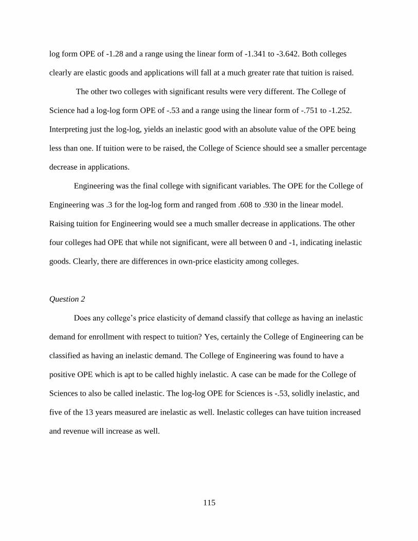
115
log form OPE of -1.28 and a range using the linear form of -1.341 to -3.642. Both colleges
clearly are elastic goods and applications will fall at a much greater rate that tuition is raised.
The other two colleges with significant results were very different. The College of
Science had a log-log form OPE of -.53 and a range using the linear form of -.751 to -1.252.
Interpreting just the log-log, yields an inelastic good with an absolute value of the OPE being
less than one. If tuition were to be raised, the College of Science should see a smaller percentage
decrease in applications.
Engineering was the final college with significant variables. The OPE for the College of
Engineering was .3 for the log-log form and ranged from .608 to .930 in the linear model.
Raising tuition for Engineering would see a much smaller decrease in applications. The other
four colleges had OPE that while not significant, were all between 0 and -1, indicating inelastic
goods. Clearly, there are differences in own-price elasticity among colleges.
Question 2
Does any college’s price elasticity of demand classify that college as having an inelastic
demand for enrollment with respect to tuition? Yes, certainly the College of Engineering can be
classified as having an inelastic demand. The College of Engineering was found to have a
positive OPE which is apt to be called highly inelastic. A case can be made for the College of
Sciences to also be called inelastic. The log-log OPE for Sciences is -.53, solidly inelastic, and
five of the 13 years measured are inelastic as well. Inelastic colleges can have tuition increased
and revenue will increase as well.

116
Question 3
Does any college’s price elasticity of demand classify that college as having an elastic
demand for enrollment with respect to tuition? The Colleges of Agriculture and Geosciences are
elastic in both the log-log and linear functional forms. Both colleges have OPE that have an
absolute value greater than 1 in both the log-log and linear forms. This indicates that decreasing
tuition for both of these would increase revenue from tuition for each.
Question 4
A tougher question to answer is if any of the colleges OPE changed over time. The linear
model is the only way to compute this as the log-log model gives the result over the entire data
set, not as specific points in time. The policy model in the linear form was significant for the
Colleges of Agriculture, Engineering, Geosciences, and Science, while the complete model was
significant only for Agriculture, Engineering, and Geosciences. For the College of Agriculture,
the complete model had the higher adjusted R-squared, so it is used for comparison purposes,
while in the other three colleges the policy model had higher adjusted R-squared values.
The College of Agriculture showed considerable variance over the thirteen years. It
peaked in 2006 with a value of -4.451 and had its lowest value in 2013 of -1.73. The College of
Geosciences also had a large range with a low of -1.341 in 2013 and a high of -3.642 in 2006.
The College of Science had a much smaller range of -.754 to -1.252. The College of
Engineering was even smaller, .608 to .930. These results show that colleges OPE do change
over time. The patterns and directions of the changes can be used to see if universities are
making the proper decisions with regards to tuition changes.

117
Question 5
What is the estimated effect charging differential tuition rates according to elasticities
would have on State U’s general revenue and enrollment? In order to attempt to answer this
question, several assumptions were made. First, for each college the policy model was used. The
log-log or linear functional forms were chosen for each college based on R-squared. The
Colleges of Agriculture, Education, Engineering, and Science used log-log, while Architecture,
Business, Geosciences, and Liberal Arts used linear. Next, two scenarios were chosen to model,
a 5% change and a 10% change. For those colleges that were inelastic, the change was an
increase in tuition. For those colleges that were elastic, the change was a decrease in tuition. The
new quantity or amount of applications was calculated by rearranging Equation 23.
OPE = % ∆ 𝑸𝒙
% ∆ 𝑷𝒙 (23)
By taking the OPE times the 5 or 10% change in tuition, a percent change in applications was
found. This was multiplied by the base applications to get new applications and multiplied by the
new tuition rate to get the new revenue. For example, in the College of Agriculture, the OPE was
-1.6004 which was multiplied by -.05 to get .08002, or an 8.002% increase in applications if
tuition is lowered by 5%. Base applications was 2702 in 2015, thus an 8% increase means they
would be 2918 with a 5% drop in tuition and with further calculation 3134 with a 10% drop in
tuition.
118
Table 39
Revenue Changes for 5 and 10% Tuition Changes Per Semester.
Apps Attend Tuition Revenue Change in Revenue
AG No Change 2702 1081 $3,302.01 $3,568,812.41
5% Drop 2918 1167 $3,136.91 $3,661,671.32 $92,858.91
10% Drop 3134 1254 $ 2,971.81 $3,725,972.39 $157,159.98
AR No Change 763 305 $3,832.94 $1,169,813.29
Increase 5 % 757 303 $4,024.59 $1,218,647.89 $48,834.60
Increase 10% 751 300 $4,216.23 $1,266,562.87 $47,914.98
BA No Change 3799 1520 $3,591.18 $5,457,157.13
Increase 5 % 3783 1513 $3,770.74 $5,705,625.43 $248,468.30
Increase 10% 3767 1507 $3,950.30 $5,951,770.92 $494,613.79
ED No Change 2466 986 $3,325.48 $3,280,253.47
Increase 5 % 2429 972 $3,491.75 $3,393,138.74 $112,885.26
Increase 10% 2393 957 $3,658.03 $3,501,154.72 $220,901.25
EN No Change 8508 3403 $3,899.31 $13,270,131.79
Increase 5 % 8635 3454 $4,094.28 $14,140,951.40 $870,819.61
Increase 10% 8761 3504 $4,289.24 $15,031,515.11 $1,761,383.32
GE No Change 481 192 $3,181.92 $612,201.41
Drop 5% 524 209 $3,022.82 $633,202.31 $21,000.90
Drop 10% 566 227 $2,863.73 $648,770.47 $36,569.07
LA No Change 3590 1436 $3,164.01 $4,543,518.36
Increase 5 % 3530 1412 $3,322.21 $4,690,759.26 $147,240.90
Increase 10% 3470 1388 $3,480.41 $4,830,387.30 $286,868.94
SC No Change 3717 1487 $3,180.87 $4,729,317.52
Increase 5 % 3619 1448 $3,339.91 $4,834,662.76 $105,345.24
Increase 10% 3521 1408 $3,498.96 $4,927,520.33 $198,202.81
119
To complete the calculations, a further assumption is needed. On average 40% of
students that apply to State U are accepted and attend the University. By taking the differences
between the base applications and the 5 or 10% changes and multiplying by .4 and the new cost
of tuition, a value for increased revenue from first-time students for each semester can be
obtained.
Of the eight colleges, Liberal Arts did not have any significant variables in the policy
model. Both Education and Sciences only had a single significant variable, while Business had
two. These four colleges were included in the forecast. Results are presented below with and
without those four colleges.
Table 39 shows the results of the calculations for both scenarios. In two colleges,
Agriculture and Geosciences, prices were dropped due to finding those colleges to be elastic
goods. For those colleges, revenue increased by $113,859.81 per semester with a 5% decrease in
tuition and by $193,729.05 per semester with a 10% decrease in tuition. Also, the number of
applicants in the two colleges by 259 or 8.13%, and 518 or 16.27% with the 5 and 10% decreases
to tuition.
Engineering was a special case. Raising tuition by 5% increased revenue for Engineering
by $870,819.61 and increasing by 10% raised revenue by $1,761,383.32 per semester.
Engineering would actually add students in both scenarios, 123 and 256 respectively.
In the other five colleges, raising tuition by 5% increased revenue by $549,889.05 per
semester and increasing by 10% raised revenue by $1,027,600.52 per semester. The number of
applications would fall by 330 students with the 5% increase and 782 with the 10%. However, as
stated, only the College of Education of these five has more than two of the six variables in the

120
policy model as significant. Removing the four colleges means if tuition is increased by 5%, the
College of Education gains $112,885.26 per semester and $220,901.25 for a 10% increase.
Table 40 shows that using elasticities to increase or decrease tuition rates on a college
basis would generate $3,294,907.47 in yearly revenue from first-time students for State U as a
whole if a 5% change was implemented and $6,407,228.26 in yearly revenue with a 10% change.
Total applications for State U would increase by 168 or .65% for a 5% change in tuition and by
337 or 1.29% for a 10% change in tuition. Table 41 shows the same information if only the four
colleges with at least 50% of the variables in the policy model significant are included. Those
four colleges could generate $2,195,129.37 per year with a 5% change and $4,352,027.22 with a
10% change.
Table 40
Total Revenue Effects for State U for 5 and 10% Tuition Changes Per Semester, All Colleges.
Apps Attend Revenue Change in Revenue
Yearly Revenue
Change
No Change 26026 10410 $36,631,205.37
5% Change 26194 10478 $38,278,659.11 $1,647,453.74 $3,294,907.47
10%
Change 26363 10545 $39,883,654.11 $3,203,614.13 $6,407,228.26

121
Table 41
Total Revenue Effects for State U for 5 and 10% Tuition Changes Per Semester, Only Significant
Colleges
Apps Attend Revenue Change in Revenue
Yearly Revenue
Change
No Change 14157 5663 $20,731,399.08
5% Change 14506 5802 $21,828,963.77 $1,097,564.69 $2,195,129.37
10%
Change 14855 5942 $22,907,412.69 $2,176,013.61 $4,352,027.22
Questions 6-9
The four secondary questions dealt with income elasticities (IE). Income was not one of
the variables found significant by the Directed Graph procedure therefore, results are only
available for the complete model. In that model, per-capita disposable income was significant for
the College of Agriculture in both log-log and linear forms, and for Geosciences and Sciences in
the log-log form. The College of Agriculture had a negative IE in both forms. In the linear form,
IE was between -5 and 06 for the first several years before dropping to -3 the last three. In the
log-log form, IE for the College of Agriculture was -1.602. Both indicate that as incomes go up,
applications in the College of Agriculture fall, making Agriculture an inferior good.
For Geosciences and Sciences, only the log-log form was significant, thus changes over
time are impossible to determine. Geosciences had an IE of 2.106 and Sciences was 1.94. Both
are positive and greater than 1, putting them into the categories of normal goods and luxury
goods. When income rises, applications in both colleges rise a great deal.

122
Answering the research questions, even with limited significant variables there are
differences in IE between colleges. Agriculture was an inferior good and the other two with
significant variables are luxury goods. No necessity goods were found among the colleges. The
final question, does income elasticity change over time, was found to be true, but only one
college had a significant variable to test.
Conclusions
The percentage of young people attending colleges in the United States continues to rise.
Coupled with the increasing population, this means that enrollment in higher education is much
greater than ever before. At the same time, federal and state appropriations for higher education
have stagnated. In response, many public institutions have increased tuition at a staggering rate.
This tuition increase has come at a universal level with no regard to economic factors such as
elasticities. In fact, some colleges and universities might benefit from decreasing tuition.
National studies have shown own-price elasticities (OPE) ranging from -.44 (Campbell &
Siegel, 1967) to -.60 (Gallet, 2007). However, these aggregated all college students and did not
differentiate between a student’s choice of college. Shin and Milton (2007) conducted a study
across a large number of universities exploring student responses to tuition increases based on
college majors. Their findings suggest that some majors do have different elasticities than others,
particularly those that have a high rate of return. This would indicate that differential tuition does
have a place in higher education.
This study attempts to further the literature by calculating elasticities at a single
institution over time on a college basis. There are some drawbacks to this type of study. Tuition
at State U has not been free to change for very long. Only in 2004 did the state legislature give

123
up tuition controls. Also, State U’s colleges have only recently started charging different
amounts to students. This limits the amount of data that is available.
With limited data come limited significant variables and results; however, the results that
are significant are very telling. Two colleges were found to have elasticities that were in the
elastic range (absolute value of OPE that is greater than one), the College of Agriculture and the
College of Geosciences. Both colleges had OPE that changed over time in a linear model and
both appear to be getting closer to -1. So while they are still very susceptible to changes in
tuition, they are becoming less so each year.
The College of Science was an inelastic good using the log-log form, with an OPE of -
.53, but was closer to a unit elastic good in the linear model. Tuition could be left alone in the
College of Science and more data collected to see which functional form is more correct. It could
also be increased due to the evidence. The College of Engineering was even more interesting
having an OPE of .3. A positive coefficient means that as costs rise, demand for Engineering
rises. Engineering can raise tuition with little fear of losing applications, in fact they might see an
increase in applications if they raised the price. The other four colleges in the study, while not
significant, had OPE in the inelastic range.
What does this all mean? The first item of significance is that there are measurable
differences between colleges in terms of own-price elasticity. This is economic proof that
differential tuition can be useful. Inelastic goods can generate more revenue with an increase in
price. Elastic goods can generate more revenue with a decrease in price. If the Colleges of
Agriculture and Geosciences were to drop their tuition 5%, their revenues would increase by
over 8%. If they dropped tuition by just 10%, their revenues would increase by over 16%. This
revenue increase comes with an increase in applications and enrollment as well. Conversely,

124
increasing tuition in the Sciences and Engineering colleges would generate more revenue.
Demand and applications in those colleges would fall, but not as much as tuition increased. This
would boost revenue a great deal.
In fact, making the recommended changes to all eight colleges, decreasing tuition in
Agriculture and Geosciences, increasing tuition in the other six, would boost revenue throughout
State U. Making a 5% change would give an additional $3.3 million in revenue from first-time
students, while changing tuition charged by 10% would boost revenue by over $6.4 million per
year. However, this does not take into account additional revenue from continuing students. In
2015, State U had nearly 31,000 continuing students in the eight colleges (State University,
2016a). Most students are not very responsive to tuition changes after they have made their
enrollment decision. Therefore, assuming retention rates remain the same, changing tuition 5%
would result in over $14 million more revenue per year, while changing tuition 10% would
generate over $28 million per year. From a pure economics standpoint, that is nearly $35 million
a year in additional revenues generated by charging the appropriate differential tuition rates.
Considering State U receives close to $400 million a year in tuition from students, $35 million is
a non-trivial amount and it seems like expanding differential tuition rates is an excellent idea.
Changing the way tuition is charged to a university-wide differential tuition rate based on
elasticities may be the best way to meet revenue shortfalls for universities, but other
considerations remain. Specifically, what is the impact of such a change on access? Particularly,
how does such a change impact access for low-socioeconomic students?
Most studies agree that all other things equal, a student with more income should be less
sensitive to changes in tuition than a student from a poorer family. Providing lower income
students with financial aid opportunities will shift their demand curves upward and bring their

125
probabilities of enrollment much closer to that of the higher income students (Heller, 1997). This
is the higher education theory of high tuition/high aid. The high tuition/high aid model revolves
around the idea that higher income families can afford higher tuition and will not care about the
higher rates. Lower income families can receive greater amounts of financial aid to offset the
cost.
There are several problems with this idea. First, the large tuition increases lead to a
"sticker shock" where low-income students are scared away because of the massive costs. They
never learn about the financial aid packages because they lack explanations of what opportunities
are available. Secondly, if aid is primarily given in loans then higher aid leads to students with
higher debt when they graduate. Many low-income students can receive grants to attend college.
Middle-income students must usually seek loans. The number of students taking out loans to pay
for education has risen by over 60% in the last decade, while the size of the debt has increased as
well.
Additionally, recent work suggests that increasing federal loan and grant programs may
not have the desired effect. Lucca, Nadauld, and Chen (2016) conducted a study in conjunction
with the Federal Reserve Bank of New York to look at the effect of increasing federal grant and
loan programs on the sticker price of tuition. They found that each additional Pell grant dollar
added about 55 cents to the tuition of students. Subsidized loans resulted in a 70% effect while
unsubsidized had a 30% effect. The authors went on to conclude that this change in sticker price
is represented in all students' net tuition, not just the relatively few that do not have grants or
loans. What results is less high tuition/high aid and more simply high tuition.
Other data suggests that the high tuition/high aid programs implemented elsewhere have
not been successful. At the University of Michigan, the number of students from households with

126
incomes between $10,000 and $74,999 has decreased by 10% since implementation of a high
tuition/high aid plan (Nishimura, 2009). Moreover, the magnitude of the effects of aid is much
less than actually reducing tuition. Two studies have found that a $1000 increase in Pell Grants
has about a 1% increase in enrollment, while a $1000 decrease in tuition increases enrollment by
as much as 6% (Cameron and Heckman, 2001); (Kane, 1994). These results are not universal. A
study of the University of California found no discernible drop in demand or access with
implementation of a high tuition/high aid plan (Ward & Douglas, 2005).
Besides effects on students from different income groups or socioeconomic backgrounds,
differential tuition and changing financial aid policies could have impacts on students from
different races. Minority students have been shown to be more responsive to financial aid offers,
with black students being more sensitive. Blacks who received grants had an 11.2 % greater
probability of enrolling than unaided blacks. To compare, a white student who received aid was
only 6.3% more likely to enroll. Hispanic students who received aid offers were no more likely
to enter college than those that did not (St. John and Noell, 1989). Similar results are reported
from studies that track the net cost of college or tuition and its effect on enrollment. Minorities
are found to have a greater sensitivity to cost than white students. Kane (1994) found that in the
bottom quartile of income levels, a $1000 increase in costs would decrease black enrollment by
22.1% and white enrollment by 11.4%. In the highest quartile, black enrollment would still
decrease by 13.2%, while white enrollment would only fall by 1.7%.
The warning inherent in these studies is that differential tuition is dangerous on its own.
Increasing tuition in those colleges with inelastic demand may force low-income students out of
those majors and into majors with more elastic demands whose tuition has been lowered. That
means low-income students that want to become engineers or accountants may not be able to

127
afford those degrees and may be forced into degrees that they may not have as much interest in,
such as liberal arts or agriculture, because the costs are less. Simply changing tuition to meet the
results of elasticity calculations could dramatically alter enrollment profiles and lock out low
socioeconomic and minority backgrounds students from higher-earning degrees.
Conversely, scholarship suggests that the standard response of high tuition/high aid may
not actually work. It does not seem to be as effective on access as lowering tuition. Sensitivity to
cost is greater in low socioeconomic students and in minorities. The challenge is to find a middle
ground. Universities cannot survive with lower tuition and less government money. If
government resources are not going to be available, tuition will have to rise. The best way to do
this is through differential tuition based on elasticities. The best way to mitigate the damaging
effects of raising tuition is to target those most affected with grant money.
Based on the results of this research, the author advises that differential tuition
formulated from calculated elasticities be considered by State U. The increase in revenues that
such a plan should generate will be large. This money can be spent on hiring new faculty, faculty
raises, increased student services, and financial aid to low-income students. All of which make
the college more competitive and more attractive to students and makes differential tuition based
on this plan appear an obvious choice. But higher revenue is not the only goal for college
administrators. Improving access for minorities and low socioeconomic students is also
important. Differential tuition is but one facet of the in the decision-making process at the
administrative level.
If differential tuition is implemented by State U, there will need to be considerations on
how the money is spent. Administrators may use the money to hire more prestigious professors
for research or make significant investments into classroom technology. While these are
128
important to consider, they might leave low-income students out of certain colleges that increase
tuition. To prevent this harm, restrictions can be included that require a large percentage of the
increased revenues be spent on institutional-level, need-based financial aid. This financial aid
should be primarily in the form of grants instead of loans to lower the risk of students graduating
with high student debt. Most of these funds should be allocated to students in those colleges that
increase their tuition rates.
Along with the dedication of funds to financial aid, a portion of the money should be
spent at State U to increase the size of the recruitment staff for low income and low
socioeconomic areas. Implementing a high tuition/high aid plan has a real chance of frightening
parents and students with low incomes away with a high sticker price. Increasing the amount of
recruiters in low income areas should allow more education on the availability of loans and
grants at the federal, state, and institutional levels; especially the new funds available as a result
of changing tuition policies. If restrictions are not put in place, administrators may use the
additional revenue in ways that strengthen the college, but damage access for low socio-
economic students.
The economics of public universities have become more important as funds from federal
and state levels continue to stagnate. University budgets promise to become one of the most
contested political battles in the near future. Charging higher amounts to students that are earning
degrees in fields that have higher wage premiums appear to be a way to increase revenues. This
approach must be coupled with realistic efforts to mitigate the effects of such an increase on low-
income students. Otherwise, differential tuition will only help in widening the stratification and
inequality among incomes in the United States.
129
Limitations
The first major limitation of the current study is the lack of available data. Only having
13 usable years of data could be considered too small a sample size. More data would give more
degrees of freedom and add validity to the study. Conversely, State U had state-mandated tuition
limits up to 2004. This means prior years may not provide any true insight into price responses
by students. Colleges in states without state-mandated tuition limits can use data back as far as
can be accumulated. Thus the model may have more use at other public universities instead of at
State U. However, the elasticities calculated at State U are only applicable at State U. The model
is universal; the results are not.
Limitations of the study also include the lack of tiered income levels in the income
variable. Breaking income into quartiles as in Kane (1994) would allow some inference on how
tuition changes impact various socioeconomic groups. The lack of directed edges from the
income variable to applications led to income being dropped from the policy model. It is possible
that using tiered levels might affect the policy model.
A potential limitation is also that the four-year competitor costs were an aggregate of all
colleges. Information was not available in an efficient form for competitor colleges at each four-
year competitor university. For instance, two of the universities used as four-year competitors do
not even have a College of Agriculture. In addition, State U's College of Business may compete
with West State U, while its College of Agriculture competes with Central U. Using expert or
survey data to determine the main four-year competitors of each college and applying the
specific cost for those colleges may provide a better measure of the four-year competitor costs
than simple aggregation. Further studies could be done to include this information, but it is
beyond the scope of this research.

130
The final limitation is the wage premium variable. Different measures of wage premium
were found and calculated, but none truly represented the eight colleges chosen. The State U
Career Center has begun to collect average starting salaries on a college and major basis, which
bodes well for this research in the future. That collection began in 2011, however, and not
enough data exists yet to include it in this study as of today.
Recommendations for Future Research
Any future research will start with mitigating the limitations of the current study. This
would mean improving the eight variables that are included in this paper. First and most basic
would be continuing the study each year as more data becomes available. More data would mean
more degrees of freedom in the statistical analysis. Second, adding the State U Career Center
data on starting salaries will improve the wage premium variable. A single wage premium cannot
model every student seeking higher education. Finding more appropriate measures of four-year
competitors costs based on colleges would also improve the included variables. Including family
income in a stratified manner might give deeper results.
With the ability of the model to determine OPE for individual colleges, the next step
becomes applying the model to individual degrees or majors. This would be a significant
undertaking and would require assistance from State U to collect application and cost data on a
major basis. The same limitations concerning four-year competitor costs would apply to majors,
but they could be overcome. Wage premiums could be calculated using State U's Career Center
calculations, which already include a starting salary for each major, albeit for only the past four
years. The result of such calculations would allow an even finer adjustment to tuition.

131
REFERENCES
Allen, R. F., & Shen, J. (1999). Some new evidence of the character of competition
among higher education institutions. Economics of Education Review, 18, 465–470.
Avila, M. (1972). Peak load pricing in higher education. Journal of Experimental
Education, 40, 6-11.
Bean, C. (1990). Endogenous growth and the pro-cyclical behavior of productivity. European
Economic Review, 34(2–3), 355–363.
Becker, G. S. (1962). Investment in human capital: A theoretical analysis. Journal of Political
Economy 70 (Supplement): 9-49.
Becker, G. S. (1993). Human capital: A theoretical and empirical analysis with special reference
to education (3rd ed.). Chicago: University of Chicago Press.
Becker, W. E. (1990). The demand for higher education. In S.A. Hoenack & E.L. Collins
(Eds.), The economics of American universities: Management, operations, and fiscal
environment. (pp. 155–188). Albany, NY: State University of New York Press.
Becker, W. E., & Waldman, D. M. (1987) The probit model. In W.E. Becker & W. Walstad
(Eds). Econometric Modeling in Economic Education Research (Edited by Boston:
Kluwer-Nijhoff.
Bessler, D. A., Yang, J., & Wongcharupan, M. (2003). Price dynamics in the international wheat
market: modeling with error correction and directed acyclic graphs. Journal of Regional
Science, 43(1), 1-33.
Bezmen T., & Depken, C. A. (1998). School characteristics and the demand for college.
Economics of Education Review, 17(2), 205-210.
Bryan G. A., & Whipple, T. W. (1995). Tuition elasticity of the demand for higher education
among current students: A pricing model. Journal of Higher Education, 66, 560-574.
Buss, C., Parker J., & Rivenburg J. (2004). Cost, quality and enrollment demand at liberal arts
colleges. Economics of Education Review, 23, 57-65.
California Community Colleges. (2011). California community colleges Chancellor Jack Scott
expresses disappointment over failure of legislators to place tax extensions on June
ballot. Retrieved from
http://www.cccco.edu/Portals/4/News/press_releases/2011/CaliforniaCommunityCollege
_PressRelease_MAR_30_2011.pdf on April 21, 2011.
Cameron, S.V., & Heckman, J. J. (2001). The dynamics of educational attainment for black,
hispanic, and white males. Journal of Political Economy, 109(3), 455-499.

132
Campbell R., & Siegal B. N. (1967). The demand for higher education in the United States,
1919-1964. The American Economic Review, 57(3), 482-494.
Canton, E., & de Jong, F. (2005). The demand for higher education in the Netherlands, 1950-
1999. Economics of Education Review, 24, 651-663.
Carbone, R., & Jenson, O. (1971). Non-resident students at state universities and
land grant colleges. College Park: University of Maryland College of Education.
Chressanthis, G. A. (1986). The impacts of tuition rate changes on college undergraduate
headcounts and credit hours over time – a case study. Economics of Education Review,
5(2), 205-217.
Ciciroa, P. (2010). Higher education funding may need decade or longer to recover, scholar
says. Retrieved on February 3, 2011 from
http://news.illinois.edu/news/10/0810higheredfunding.html
Chopra, R. (2010). Student debt swells, federal loans now top a trillion. Retrieved on September
28, 2014 from http://www.consumerfinance.gov/newsroom/student-debt-swells-federal-
loans-now-top-a-trillion/
Clotfelter, C. T. (1991). Demand for undergraduate education. In C.T. Clotfelter,
R. Ehrenberg, M. Getz, & J. J. Siegfried (Eds.), Economic Challenges in Higher
Education. Chicago: University of Chicago Press.
College Board (2010). Education pays 2010. Retrieved from
http://trends.collegeboard.org/education_pays on April 20, 2011.
College Board (2013). Trends in college pricing 2013. Retrieved from
http://trends.collegeboard.org/sites/default/files/college-pricing-2013-full-report-
140108.pdf on September 30, 2014
Corazzini, A. J., Dugan, D. J., & Grabowski, H. G. (1972). Determinants and distributional
aspects of enrollment in U.S. higher education. The Journal of Human Resources, 7(1),
39-59.
Curs, B. R., & Singell, L. D. (2010). Aim high or go low? Pricing strategies and enrollment
effects when the net price elasticity varies with need and ability. The Journal of Higher
Education, 81(4), 515-543.
Derochers, D., Lenihan, C., & Wellman, J. (2010). Trends in College Spending, 1998-2008 (p.
56). Delta Project on Postsecondary Education Costs, Productivity, and Accountability.

133
DesJardins, S. L., & Bell, A. (2006). Using economic concepts to inform enrollment
management. In R. K. Toutkoushian & M. B. Paulsen (Eds.), New directions for
institutional research: No. 132. Applying economics to institutional research. San
Francisco: Jossey-Bass.
DesJardins, S. L., & Toutkoushian, R. K. (2005). Are students really rational? The development
of rational thought and its application to student choice. . In J. C. Smart (Ed.), Higher
education: Handbook of theory and research, Volume 20 (pp. 191-240). Dordrecht, The
Netherlands: Kluwer Academic Publishers.
Dougan, W. R. (1982). Giffen goods and the law of demand. The Journal of Political Economy,
90(4), 809-815.
Dynarski, S. M. (2000). Hope for whom? Financial aid for the middle class and its impact on
college attendance. National Tax Journal. 53(3), 629-61.
Educated Risk. (2016). Student loan analysis and research. Retrieved from
http://educatedrisk.org/analysis/student-loan-interest-rates-current-and-historical on June
20, 2016.
Epple, D., Romano, R., & Sieg, H. (2006). Admission, tuition, and financial aid policies in the
market for higher education. Econometrica, 74(4),885-928.
Ehrenberg, R. G., & Sherman D. R. (1984). Optimal financial aid policies for a selective
university. The Journal of Human Resources, 19(2), 202-230.
Fuller, W. (1976). Introduction to Statistical Time Series. New York. John Wiley and Sons.
Gallet, C. (2007). A comparative analysis of the demand for higher education: Results from a
meta-analysis of elasticities. Economics Bulletin, 9(7), 1-14.
Galper, H., & Dunn, R. M. (1969). A short-run demand function for higher education in the
United States. The Journal of Political Economy, 77(5), 765-777.
Geiger, D., Verma, T., & Pearl, J. (1990). Identifying independence in bayesian
networks. Networks, 20(5), 507-534.
Ghali, M., Miklius, W., & Wadak, R. (1977). The demand for higher education facing an
individual institution. Higher Education, 6(4), 477-487.
Granger, C. W. (1969). Investigating causal relations by econometric models and cross-spectral
methods. Econometrica: Journal of the Econometric Society, 424-438.
Gullason, E. T. (1989) The consumption value of schooling: an empirical estimate of one aspect.
The Journal of Human Resources, 24, 287–298.

134
Haigh, M. S., & Bessler, D. A. (2004). Causality and price discovery: An application of directed
acyclic graphs. The Journal of Business, 77(4), 1099-1121.
Hansen, W. L. (1970). Income distribution effects of higher education. American Economic
Review, 60, 335-40.
Heller, D. E. (1997). Student price response in higher education: An update to Leslie and
Brinkman. Journal of Higher Education, 68, 624-659.
Heller, D. E. (2006). State support of higher education: Past, present, and future. In D. M. Priest
& E. P. St. John (Eds.) Privatization and public universities (pp. 11-37). Bloomington,
IN: Indiana University Press.
Heller, D. E. (2001). Trends in public colleges and universities. In D.E. Heller (Ed.), The states
and public higher education policy. pp. 11-38. Baltimore: Johns Hopkins University
Press.
Henderson, D. R. (2008). Demand. The Concise Encyclopedia of Economics. Retrieved on
February 10, 2011 from http://www.econlib.org/library/Enc/Demand.html
Hight, J. E. (1975). The demand for higher education in the U.S. 1927-1972: The public and
private institutions. The Journal of Human Resources, 10(4), 512-520.
Hilmer, M. J. (1998). Post-secondary fees and the decision to attend a university or a community
college. Journal of Public Economics, 67, 329-348.
Hoenack, S. A. (1982).Pricing and efficiency in higher education. Journal of Higher Education,
53, 403-18.
Immerwahr, J., Johnson, J, Ott, A., & Rochkind, J. (2010). Squeeze play 2010: Continued public
anxiety on cost, harsher judgments on how colleges are run. Report from the National
Center for Public Policy; Public Agenda.
Jackson, G. A., & Weathersby, G. B. (1975). Individual demand for higher education: A review
and analysis of recent empirical studies. Journal of Higher Education, 46(6), 623-652.
Kane, T. J. (1994). College entry by blacks since 1970: The role of college costs, family
background, and the returns to education. Journal of Political Economy, 102(5), 878–
911.
Leslie, L. L., & Brinkman, P. T. (1987). Student price response in higher education: The student
demand studies. Journal of Higher Education, 58, 181-204.
Lingenfelter, P. E. (2009). What next? Retrieved on January 28, 2011 from
http://www.sheeo.org/finance/shef/FY2009tables/WhatNext.pdf

135
Lucca, D. O., Nadauld, T., & Chen, K. (2016). Credit supply and the rise in college tuition:
Evidence from the expansion in federal student aid programs. Staff Report no. 733.
Federal Reserve Bank of New York.
Marshall, A. (1920). Principles of economics. 8th
ed. London: Macmillan and Col, Ltd.
McMahon, W. W., & Wagner, A. P. (1982). The monetary returns to education as partial social
efficiency criteria. In W.W. McMahon and T.G. Geske (Eds.), Financing education:
Overcoming inefficiency and inequity. Urbana, IL: University of Illinois Press.
McPherson, M. S., & Schapiro, M. O. (1991). Does student aid affect college enrollment? New
evidence on a persistent controversy. The American Economic Review, 81(1), 309-318.
Menzies, M. D. (2004). Investigating the growth of the Texas cattle feeding industry and the
possible need for additional slaughter capacity. (Master’s thesis.) Texas A&M
University, College Station, TX.
Moore, H. L. (1914). Economic cycles: Their law and cause. The Macmillan Company. New,
York, NY.
Moore, R. L., Studenmund, A. H., & Slobko, T. (1991). The effect of the financial aid package
on the choice of a selective college. Economics of Education Review, 10(4), 311-321.
Murphy, K. M., & Welch, F. (1989). Wage premiums for college graduates: Recent growth and
possible explanations. Educational Researcher, 18(4), 17-26.
Noorbakhsh, A., & Culp, D. (2002). The demand for higher education: Pennsylvania’s
nonresident tuition experience. Economics of Education Review, 21, 277-286.
O'Connell, J. F., & Perkins, G. M. (2003). The economics of private liberal arts
colleges. The Journal of Business. 76(3), 499-514.
Parker, J., & Summers, J. (1993). Tuition and enrollment yield at selective liberal arts colleges.
Economics of Education Review, 12(4), 311-324.
Paulsen, M. B., & Toutkoushian, R. K. (2008). Economic models and policy analysis in higher
education: A diagrammatic exposition. In J. C. Smart (Ed.), Higher education: Handbook
of theory and research (Vol. XXIII, pp. 1–48). Dordrecht, the Netherlands: Springer.
Pearl, J. (1995). Causal diagrams for empirical research. Biometrika, 82(4), 669-688.
Pearl, J. (2009). Causality. Cambridge University Press.
Quinn, R., & Price, J. (1998). The demand for medical education: An augmented human capital
approach. Economics of Education Review, 17(3), 337-347.

136
Richardson, J. W., Schumann, K. D, & Feldman, P. A. (2008). Simetar© 2008 Simulation &
econometrics to analyze risk. Simetar, Inc. College Station, TX.
Rothschild, M., & White, L. J. (1995). The analytics of the pricing of higher education and other
services in which the customers are inputs. The Journal of Political Economy, 103(3),
573-586.
Rusk, J. J., & Leslie, L. L. (1978). The setting of tuition in public higher education. The Journal
of Higher Education, 49(6), 531-547.
Saint-Paul, G. (1993). Productivity growth and the structure of the business cycle. European
Economic Review, 37(4), 861–890.
Saupe, J., & Stephens, W. (1974). Differential by level and per credit student charges in
major public universities.. Washington DC: Education Resources Information Center.
(ERIC Document Reproduction Service No. ED131739).
Savoca, E. (1990) Another look at the demand for higher education: Measuring the price
sensitivity of the decision to apply to college. Economics of Education, 9(2), 123-134.
Scheines, R., Sprites P., Glymour, C., & Meek, C. (1994). Tetrad II: User’s Manual and
Software. Hillsdale, New Jersey: Lawrence Erlbaum Associates, Inc.
Schultz, T. W. (1961). Investment in human capital. American Economic Review, 51, 1-17.
Shin, J. C., & Milton, S. (2006). Rethinking tuition effects on enrollment in public four-year
colleges and universities. The Review of Higher Education, 29(2), 213-237.
Shin, J. C., & Milton, S. (2007). Student response to tuition increase by academic majors:
empirical grounds for a cost-related tuition policy. Higher Education, 55,719-734.
Simone, S. (2010). Tuition and fee differentiation at degree granting postsecondary education
institutions. An AIR/NCES Data Policy Fellowship Report. National Center for Education
Statistics, Washington DC.
Spence, M. (1973). Job market signaling. Quarterly Journal of Economics, 87, 355-374.
Suppes, P. (1970). A Probabilistic Theory of Causality. Amsterdam: North Holland.
State University (2016a). Data and reports/students. Data and Research Services, State
University. Retrieved on June 15, 2016 from http://dars.tamu.edu/Data-and-
Reports/Student#applied.
State University (2016b). Student Business Services. Retrieved on June 20, 2016 from
http://sbs.tamu.edu/accounts-billing/tuition-fees/.

137
State University (2016c). Career Center. Retrieved on July 15, 2016 from
http://moses.tamu.edu/ccsurveyreports/SurveyReport.aspx.
State University (2016d). Mays Business School Rankings. Retrieved on December 10, 2016
from http://mays.tamu.edu/rankings/.
State University (2016e). State U Engineering ranked 7th
among public universities in latest
graduate survey. Retrieved on December 10, 2016 from
http://engineering.tamu.edu/news/2016/03/16/texas-am-engineering-ranked-7th-among-
public-universities-in-latest-graduate-survey.
State Higher Education Coordinating Board (2016). Tuition and fee data. Retrieved on June 15,
2016 from http://www.thecb.state.tx.us/index.cfm?objectid=D921014A-DF8A-5DB2-
0CAA9DAC3DF3D384.
The Washington Monthly. (2010). The Washington monthly national university rankings. The
Washington Monthly. Retrieved on April 15, 2011 from
http://www.washingtonmonthly.com/college_guide/rankings_2010/national_university_r
ank.php
U.S. Bureau of Economic Analysis. (2016). Per capita personal income. Retrieved from FRED,
Federal Reserve Bank of St. Louis https://research.stlouisfed.org/fred2/series/TXPCPI,
June 17, 2016.
U.S. Census Bureau (2016). Current Population Survey. Retreived from
http://www.census.gov/cps/data/cpstablecreator.html on June 25, 2016
U.S. Department of Education. (2013). Digest of Education Statistics, 2012. National Center for
Education Statistics, NCES 2014-015.
Vasigh, B., & Hamzaee R.G. (2004). Testing sensitivity of student enrollment with respect to
tuition at an institution of higher education. International Advances in Economic
Research, 10, 133-149.
Ward, D., & Douglass, J. A. (2005). The dynamics of variable fees: Exploring institutional and
public policy responses. Research and Occasional Paper Series (CSHE.5.05). University
of California, Berkeley.
Weinberg, I. (1978). Financing higher education in 1980s and beyond. Washington, DC:
National Institute of Education.
Wetzel, J. O’Toole, D., & Peterson, S. (1998). An analysis of student enrollment demand.
Economics of Education Review, 17(1), 47-54.
Windham, D. M. (1972). Tuition, the capital market, and the allocation of subsidies to college
students. School Review, 80, 603-18.

138
Winston, G. C. (1999). Subsidies, hierarchy, and peers: The awkward economics of higher
education. The Journal of Economic Perspectives, 13(1), 13-36.
Woodhall, M. (1995). Human capital concepts. In M. Carnoy (ed.), International encyclopedia of
economics of education (2nd ed.). Tarrytown, NY: Elsevier
Yanikoski. R. A., & Wilson, R. F. (1984). Differential pricing of undergraduate education. The
Journal of Higher Education. 55(6), 735-750.

139
3APPENDIX A
DIRECTED ACYCLIC GRAPH THEORY
The theory of directed acyclic graphs begins with the concept of causality. Granger
causality states that a cause precedes its associated effect, while an effect does not precede its
cause (Granger, 1969). A directed graph is a picture that represents causal flow between or
among a set of variables. Letters are used to represent variables and lines (edges) with
directional arrowheads at one end to represent causal flows. A graph with directed edges is
called a directed graph (Haigh & Bessler, 2003). An acyclic graph has no path that leads away
from a variable only to return to that same variable. For example, the path ABCA is
cyclic as it moves from A to B, then returns to A by way of C (Bessler, et al., 2003). A variable
is called a collider if arrows converge on it. Consider the path ABC; the vertex B is a
collider while vertices A and C are directionally separated. To understand directional-separation,
conditionality must be understood.
An example of conditional and unconditional association or correlation is a set of three
variables M, N, and O. A relationship may exist such that MNO. This suggests that
unconditional association between M and O is non-zero, but conditional association between M
and O is zero because of the common cause, N. This common cause screens off associations
between joint effects. Conversely, if M and O cause N such as, MNO, then the
unconditional association between M and O is zero while the conditional association between M
3 Reprinted with permission from Menzies, M.D. (2004). Investigating the growth of the Texas cattle feeding
industry and the possible need for additional slaughter capacity. (Master’s thesis.) Texas A&M University,
College Station, TX.

140
and O is non-zero due to the common effect, N. Thus demonstrating that common effects do not
screen off associations between joint causes (Bessler et al., 2003).
Direction-separation (d-separation) is a graphical characterization of conditional
independence (Pearl, 1995). D-separation can be understood by using three subsets of variables
D, E, and F in a graph G. Let p be any path between a variable in set D and a variable in set F.
For any p, the set E blocks p if there is a variable k on the path that satisfies one of the following
conditions: (i) variable k has converging arrows along p and neither k or any of its descendents
are in E; or (ii) k does not have converging arrows along p and k is a member of set E. Set E is
thus said to d-separate set D from set F on graph G if and only if E blocks every path from a
variable in D to a variable in F (Pearl, 1995). Continuing the example, if G is a directed acyclic
graph with vertex set V, if J and K are in V as is H, then G linearly implies the correlation
between J and K conditional on H is zero, if and only if J and K are d-separated given H (Geiger,
Verma, & Pearl, 1990).
To illustrate component (i) above, return to the path ABC. Vertex B is a collider as
described, A and C are d-separated. If B is conditioned upon, however, the information flow
from A to C is opened up. Conditioning on B makes A and C directionally connected (d-
connected). Adding a fourth variable, D, to the original path as below gives a new path
ABC
D
If D is now conditioned on instead of B, the flow between A and C is also opened, demonstrating
(i) (Bessler et al., 2003).

141
If the information flow is not characterized by converging arrows, as above, but rather by
diverging arrows, then the d-separation condition is different. This is given by component (ii)
above. Consider from above, MNO, where N is the common cause of M and O. Again the
unconditional correlation between M and O will be non-zero, because of the common cause N.
If N is conditioned upon, the correlation between M and O will disappear. Conditioning on the
common cause blocks the flow of information between common effects. M and O are d-
connected in an unconditional sense because they have a common cause, while conditioning on
N leaves M and O d-separated (Pearl, 2009).
Another application of component (ii) above is in the causal chain. If M causes N and N
causes O then the following results: MNO. The unconditional correlation between M and
O will be non-zero, but the correlation between M and O conditional on N will be zero. For
causal chains, the end points (M and O) are not d-separated, whereas conditioning on the middle
vertex N leads to the endpoints being d-separated.
The notion of d-separation has been incorporated into an algorithm (PC algorithm) by
Sprites, Glymour, and Scheines (1994). PC algorithm is an ordered set of commands that begin
with an undirected, unrestricted graph with every variable connected with every other variable
and uses a step-wise procedure to remove edges between variables and direct the causal flow
among the variables.
The general procedure of the PC algorithm begins with a complete undirected graph, G
on the vertex set M. Lines (edges) are removed sequentially based on zero correlation or partial
correlation (conditional correlation). Fisher’s z is used to test whether conditional correlations
are significantly different from zero. Fisher’s z is defined as:

142
z(p(i,j|k),n) = [1/2(n-|k|-3)1/2
]ln {[|1+p(i,j|k)|] * [|1-p(i,j|k)|]-1
}
Where n is the number of observations used to estimate the correlations, p(i,j|k) is the population
correlation between series, i and j conditional on series k (removing the influence of series k on
each i and j), and |k| is the number of variables in k (that we condition on). If i, j, and k are
normally distributed and r(i,j|k)is the sample conditional correlation of i and j given k, the
distribution of z(p(i,j|k),n)-z(r(i,j|k),n) is standard normal (Bessler et al., 2003).
The remaining variables are directed then using the idea of sepset, which can be defined
as: The conditioning variable(s) on removed edges between two variables is called the sepset of
the variables whose edge has been removed (for vanishing zero order conditioning information
the sepset is the empty set) (Haigh & Bessler, 2003). Edges are thus directed by considering
triples A B C, such that A and B are adjacent, as are B and C, but A and C are not. Edges
between the triples are directed as such: A B C as ABC if B is not in the sepset of A
and C. If AB, B and C are adjacent, A and C are not adjacent, and there is no arrowhead at B,
then orient B C ad BC. If there is a directed path from A to B and an edge between A and
B, then direct A B as AB (Bessler, et al., 2003).
There are three requirements that can be violated when using directed graphs to
correspond to the random assignment experimental models (the counterfactual random variable
model) developed by Holland. The first of these requirements is the need to have a causally
sufficient set of variables. This refers to not omitting any variable that in fact causes any
variable in the study. If X causes both Y and Z and X is omitted, then an apparent causal flow
from Y to Z may be due to X and would thus be spurious (Suppes, 1970).

143
The second requirement is that the graph needs to be constrained to causal flows that
respect a causal Markov condition. If X causes Y and Y causes X, the underlying probability
distribution can by factored on X, Y, and Z as:
Pr(X,Y,Z) = Pr(X)*Pr(Y|X)*Pr(Z|Y)
(2)
Put another way, the causal flow that is being uncovered must respect the genealogy condition
that one need only condition on its parents in order to fully capture the probability distribution
generating any variable. One need not condition on grandparents, siblings, or any other relative
(Bessler, et al., 2003).
The final condition is that the probabilities that are being captured by graph G are faithful
to G if X and Y are dependent if and only if there is an edge between X and Y. These three can
all be violated, thus any result that is obtained based on observational data must be viewed with
some caution. Failure to include a relevant variable may lead to an edge between two variables
when in fact a third omitted variable is causing both. Failure of the Markov condition would
lead to ignoring statistical dependency even in experimental designs. Failure of the third
condition, the faithfulness condition, can occur if parameters between causes happen to be of the
precise magnitude to cancel one another. Care must be taken to ensure that the three
requirements are met, especially the first.

144
APPENDIX B
COLLEGE CORRELATION MATRICES
Table B1
College of Agriculture Correlation Matrix
APPS TUI FEES 4YR 2YR INC UR FS WP
APPS 1.0000
TUI 0.8127 1.0000
FEES -0.0124 0.3581 1.0000
4YR 0.8732 0.9508 0.2969 1.0000
2YR 0.9163 0.9187 0.1798 0.9824 1.0000
INC 0.9004 0.9309 0.1983 0.9601 0.9602 1.0000
UR 0.1595 -0.0223 -0.0522 0.1838 0.2461 -0.0002 1.0000
FS -0.4480 -0.0474 0.3846 -0.2310 -0.3547 -0.1985 -0.7480 1.0000
WP 0.5106 0.4433 0.0724 0.6234 0.6659 0.5338 0.6557 -0.5571 1.0000
Table B2
College of Architecture Correlation Matrix
APPS TUI FEES 4YR 2YR INC UR FS WP
APPS 1.0000
TUI 0.8311 1.0000
FEES 0.3441 0.3686 1.0000
4YR 0.8837 0.9395 0.4598 1.0000
2YR 0.9255 0.9344 0.4074 0.9824 1.0000
INC 0.9061 0.9323 0.3910 0.9601 0.9602 1.0000
UR 0.1988 0.0097 0.0892 0.1838 0.2461 -0.0002 1.0000
FS -0.4789 -0.1494 0.0772 -0.2310 -0.3547 -0.1985 -0.7480 1.0000
WP 0.6251 0.4399 0.5562 0.6234 0.6659 0.5338 0.6557 -0.5571 1.0000

145
Table B3
College of Business Correlation Matrix
APPS TUI FEES 4YR 2YR INC UR FS WP
APPS 1.0000
TUI 0.7406 1.0000
FEES 0.1411 0.5336 1.0000
4YR 0.8109 0.9333 0.4598 1.0000
2YR 0.8782 0.8942 0.4074 0.9824 1.0000
INC 0.8760 0.9167 0.3910 0.9601 0.9602 1.0000
UR 0.0458 0.0223 0.0892 0.1838 0.2461 -0.0002 1.0000
FS -0.3858 -0.0921 0.0772 -0.2310 -0.3547 -0.1985 -0.7480 1.0000
WP 0.4207 0.5533 0.5562 0.6234 0.6659 0.5338 0.6557 -0.5571 1.0000
Table B4
College of Education Correlation Matrix
APPS TUI FEES 4YR 2YR INC UR FS WP
APPS 1.0000
TUI 0.8983 1.0000
FEES 0.2683 0.3825 1.0000
4YR 0.9008 0.9806 0.4598 1.0000
2YR 0.9394 0.9604 0.4074 0.9824 1.0000
INC 0.9200 0.9634 0.3910 0.9601 0.9602 1.0000
UR 0.1496 0.0544 0.0892 0.1838 0.2461 -0.0002 1.0000
FS -0.4007 -0.1395 0.0772 -0.2310 -0.3547 -0.1985 -0.7480 1.0000
WP 0.5177 0.5146 0.5562 0.6234 0.6659 0.5338 0.6557 -0.5571 1.0000

146
Table B5
College of Engineering Correlation Matrix
APPS TUI FEES 4YR 2YR INC UR FS WP
APPS 1.0000
TUI 0.9485 1.0000
FEES 0.1751 0.3911 1.0000
4YR 0.8727 0.9597 0.4598 1.0000
2YR 0.9042 0.9620 0.4074 0.9824 1.0000
INC 0.9132 0.9444 0.3910 0.9601 0.9602 1.0000
UR -0.0018 0.0789 0.0892 0.1838 0.2461 -0.0002 1.0000
FS -0.2737 -0.2107 0.0772 -0.2310 -0.3547 -0.1985 -0.7480 1.0000
WP 0.4007 0.5065 0.5562 0.6234 0.6659 0.5338 0.6557 -0.5571 1.0000
Table B6
College of Geosciences Correlation Matrix
APPS TUI FEES 4YR 2YR INC UR FS WP
APPS 1.0000
TUI 0.8193 1.0000
FEES 0.3152 0.4753 1.0000
4YR 0.9289 0.9589 0.4598 1.0000
2YR 0.9671 0.9206 0.4074 0.9824 1.0000
INC 0.9188 0.9314 0.3910 0.9601 0.9602 1.0000
UR 0.3453 -0.0053 0.0892 0.1838 0.2461 -0.0002 1.0000
FS -0.5280 -0.0372 0.0772 -0.2310 -0.3547 -0.1985 -0.7480 1.0000
WP 0.7049 0.4693 0.5562 0.6234 0.6659 0.5338 0.6557 -0.5571 1.0000

147
Table B7
College of Liberal Arts Correlation Matrix
APPS TUI FEES 4YR 2YR INC UR FS WP
APPS 1.0000
TUI 0.8619 1.0000
FEES 0.3135 0.4802 1.0000
4YR 0.9290 0.9598 0.4598 1.0000
2YR 0.9651 0.9206 0.4074 0.9824 1.0000
INC 0.9450 0.9311 0.3910 0.9601 0.9602 1.0000
UR 0.2108 -0.0026 0.0892 0.1838 0.2461 -0.0002 1.0000
FS -0.4296 -0.0356 0.0772 -0.2310 -0.3547 -0.1985 -0.7480 1.0000
WP 0.6353 0.4733 0.5562 0.6234 0.6659 0.5338 0.6557 -0.5571 1.0000
Table B8
College of Science Correlation Matrix
APPS TUI FEES 4YR 2YR INC UR FS WP
APPS 1.0000
TUI 0.7876 1.0000
FEES 0.4461 0.4756 1.0000
4YR 0.9142 0.9589 0.4598 1.0000
2YR 0.9367 0.9206 0.4074 0.9824 1.0000
INC 0.8735 0.9314 0.3910 0.9601 0.9602 1.0000
UR 0.4294 -0.0051 0.0892 0.1838 0.2461 -0.0002 1.0000
FS -0.4780 -0.0371 0.0772 -0.2310 -0.3547 -0.1985 -0.7480 1.0000
WP 0.8095 0.4696 0.5562 0.6234 0.6659 0.5338 0.6557 -0.5571 1.0000

148
APPENDIX C
DIRECTED ACYCLIC GRAPHS
Figure C1. Directed Graph for AG College.
Figure C2. Directed Graph for AR College.
4YR
2YR
APPS
TUI
4YR
2YR
APPS
TUI

149
Figure C3. Directed Graph for ED College.
Figure C4. Directed Graph for EN College.
4YR
2YR
APPS
TUI
4YR
2YR
APPS
TUI

150
Figure C5. Directed Graph for GE College.
Figure C6. Directed Graph for LA College.
4YR
2YR
APPS
TUI
4YR
2YR
APPS
TUI

151
Figure C7. Directed Graph for BA College.
Figure C8. Directed Graph for SC College.
4YR
2YR
APPS
TUI
4YR
2YR
APPS
TUI


