
arX
iv:1
503.
0901
1v5
[m
ath.
ST]
17
Apr
201
8
Asymptotic Theory of Bayes Factor in Stochastic Differential
Equations: Part I
Trisha Maitra and Sourabh Bhattacharya∗
Abstract
Research on asymptotic model selection in the context of stochastic differential equations (SDE’s)
is almost non-existent in the literature. In particular, when a collection of SDE’s is considered, the
problem of asymptotic model selection has not been hitherto investigated. Indeed, even though the
diffusion coefficients may be considered known, questions on appropriate choice of the drift func-
tions constitute a non-trivial model selection problem.
In this article, we develop the asymptotic theory for comparisons between collections of SDE’s
with respect to the choice of drift functions using Bayes factors when the number of equations (indi-
viduals) in the collection of SDE’s tend to infinity while the time domains remain bounded for each
equation. Our asymptotic theory covers situations when the observed processes associated with the
SDE’s are independently and identically distributed (iid), as well as when they are independently
but not identically distributed (non-iid). In particular, we allow incorporation of available time-
dependent covariate information into each SDE through a multiplicative factor of the drift function;
we also permit different initial values and domains of observations for the SDE’s.
Our model selection problem thus encompasses selection of a set of appropriate time-dependent
covariates from a set of available time-dependent covariates, besides selection of the part of the drift
function free of covariates.
For both iid and non-iid set-ups we establish almost sure exponential convergence of the Bayes
factor.
Furthermore, we demonstrate with simulation studies that even in non-asymptotic scenarios
Bayes factor successfully captures the right set of covariates.
Keywords: Bayes factor consistency; Kullback-Leibler divergence; Martingale; Stochastic differ-
ential equations; Time-dependent covariates; Variable selection.
1 Introduction
In statistical applications where “within” subject variability is caused by some random component vary-
ing continuously in time, stochastic differential equations (SDE’s) have important roles to play for
modeling the temporal component of each individual. The inferential abilities of the SDE’s can be
enhanced by incorporating covariate information available for the subjects. In these time-dependent
situations it is only natural that the available covariates are also continuously varying with time. Exam-
ples of statistical applications of SDE-based models with time-dependent covariates are Oravecz et al.
(2011), Overgaard et al. (2005), Leander et al. (2015), the first one also considering the hierarchical
Bayesian paradigm.
Unfortunately, asymptotic inference in systems of SDE based models consisting of time-varying
covariates seem to be rare in the statistical literature, in spite of their importance. So far random ef-
fects SDE models have been considered for asymptotic inference, without covariates. We refer to
Delattre et al. (2013) for a brief review, who also undertake theoretical and classical asymptotic investi-
gation of a class of random effects models based on SDE’s. Specifically, they model the i-th individual
by
dXi(t) = b(Xi(t), φi)dt+ σ(Xi(t))dWi(t), (1.1)
where, for i = 1, . . . , n, Xi(0) = xi is the initial value of the stochastic process Xi(t), which is as-
sumed to be continuously observed on the time interval [0, Ti]; Ti > 0 assumed to be known. The
function b(x, ϕ), which is the drift function, is a known, real-valued function on R × Rd (R is the real
line and d is the dimension), and the function σ : R 7→ R is the known diffusion coefficient. The
∗Trisha Maitra is a PhD student and Sourabh Bhattacharya is an Associate Professor in Interdisciplinary Statistical Research
Unit, Indian Statistical Institute, 203, B. T. Road, Kolkata 700108. Corresponding e-mail: [email protected].
1
SDE’s given by (1.1) are driven by independent standard Wiener processes {Wi(·); i = 1, . . . , n},
and {φi; i = 1, . . . , n}, which are to be interpreted as the random effect parameters associated with
the n individuals, which are assumed by Delattre et al. (2013) to be independent of the Brownian mo-
tions and independently and identically distributed (iid) random variables with some common distri-
bution. For the sake of convenience Delattre et al. (2013) (see also Maitra and Bhattacharya (2016)
and Maitra and Bhattacharya (2015)) assume b(x, φi) = φib(x). Thus, the random effect is a multi-
plicative factor of the drift function. In this article, we generalize the multiplicative factor to include
time-dependent covariates.
In the case of SDE-based models, proper specification of the drift function and the associated prior
distributions demand serious attention, and this falls within the purview of model selection. Moreover,
when (time-varying) covariate information are available, there arises the problem of variable selection,
that is, the most appropriate subset from the set of many available covariates needs to be chosen. As is
well-known (see, for example, Kass and Raftery (1995)), the Bayes factor (Jeffreys (1961)) is a strong
candidate for dealing with complex model selection problems. Hence, it is natural to consider this crite-
rion for model selection in SDE set-ups. However, dealing with Bayes factors directly in SDE set-ups
is usually infeasible due to unavailability of closed form expressions, and hence various numerical ap-
proximations based on Markov chain Monte Carlo, as well as related criteria such as Akaike Information
Criterion (Akaike (1973)) and Bayes Information Criterion (Schwarz (1978)), are generally employed
(see, for example, Fuchs (2013), Iacus (2008)). But quite importantly, although Bayes factor and its
variations find use in general SDE models, in our knowledge covariate selection in SDE set-ups has
not been addressed so far.
Moreover, asymptotic theory of Bayes factors in SDE contexts, with or without covariates, is still
lacking (but see Sivaganesan and Lingham (2002) who asymptotically compare three specific diffusion
models in single equation set-ups using intrinsic and fractional Bayes factors). In this paper, our goal
is to develop an asymptotic theory of Bayes factors for comparing different sets of SDE models. Our
asymptotic theory simultaneously involves time-dependent covariate selection associated with a mul-
tiplicative part of the drift function, in addition to selection of the part of the drift function free of
covariates. The asymptotic framework of this paper assumes that the number of individuals tends to
infinity, while their domains of observations remain bounded.
It is important to clarify that the diffusion coefficient is not associated with the question of model
selection. Indeed, it is already known from Roberts and Stramer (2001) that when the associated con-
tinuous process is completely observed, the diffusion coefficient of the relevant SDE can be calculated
directly. Moreover, two diffusion processes with different diffusion coefficients are orthogonal. Conse-
quently, we assume throughout that the diffusion coefficient of the SDE’s is known.
We first develop the model selection theory using Bayes factor in general SDE based iid set-up; note
that the iid set-up ensues when there is no covariate associated with the model and when the initial values
and the domains of observations are the same for every individual. The model selection problem in iidcases is essentially associated with the choice of the drift functions with no involvement of covariate
selection. We then extend our theory to the non-iid set-up, consisting of time-varying covariates and
different initial values and domains of observations. Here model selection involves not only selection of
the part of the drift functions free of the covariates, but also the subset of important covariates from a set
of available covariates.
Specifically, we prove almost sure exponential convergence of the relevant Bayes factors in our
set-ups. Assuming the iid set-up we develop our asymptotic theory based on a general result already
existing in the literature. However, for the non-iid situation we first develop a general theorem which
may perhaps be of independent interest, and prove almost sure exponential convergence of the Bayes
factor in our non-iid SDE set-up as a special case of our theorem.
It is important to note that (which we also clarify subsequently in Section 2.6), that in the asymp-
totic framework of this paper, where the domains of observations remain bounded for the individuals,
incorporation of random effects does not make sense from the asymptotic perspective. For this reason
we include random effects in our paper Maitra and Bhattacharya (2018b), where we assume that even
2

the domains of observations are allowed to increase indefinitely.
The rest of our article is structured as follows. In Section 2 we formalize the problem of model
selection in our aforementioned asymptotic framework. We then present the necessary assumptions and
results in Section 3. In Section 4 we investigate convergence of the Bayes factor when the SDE models
being compared form an iid system of equations. In Section 5 we develop a general asymptotic theory of
Bayes factors in the non-iid situation, and then in Section 6 we investigate exponential convergence of
the Bayes factor when the system of SDE’s are non-iid. In Section 7 we demonstrate with simulation
studies that Bayes factor yields the correct covariate combination for our SDE models even in non-
asymptotic cases. We provide a brief summary of this article and make concluding remarks in Section
8.
The proofs of our lemmas and theorems are provided in the supplementary document whose sections
will be referred to in this article by the prefix “S-”.
2 Formalization of the model selection problem in the SDE set-up
Our assumptions (H2′) in Section 3 ensure that our considered systems are well defined and we are able
to compute the exact likelihood. We consider the filtration (FWt , t ≥ 0), where FW
t = σ(Wi(s), s ≤ t).Each process Wi is a (FW
t , t ≥ 0)-adapted Brownian motion.
In connection with model selection we must analyze the same data set with respect to two different
models. So, although the distribution of the underlying stochastic process under the two models are
different, to avoid notational complexity we denote the process by Xi(t) under both the models, keeping
in mind that the distinction becomes clear from the context and also by the model-specific parameters.
2.1 The structure of the SDE models to be compared
Now, let us consider the following two systems of SDE models for i = 1, 2, . . . , n:
dXi(t) = φi,ξ0(t)bβ0(Xi(t))dt + σ(Xi(t))dWi(t) (2.1)
and
dXi(t) = φi,ξ1(t)bβ1(Xi(t))dt + σ(Xi(t))dWi(t) (2.2)
where, Xi(0) = xi is the initial value of the stochastic process Xi(t), which is assumed to be continu-
ously observed on the time interval [0, Ti]; Ti > 0 for all i and assumed to be known. We assume that
(2.1) represents the true model and (2.2) is any other model. In the above equations, for j = 0, 1, ξj and
βj denote the sets of parameters associated with the true model and the other model.
2.2 Incorporation of time-varying covariates
We model φi,ξj (t) for j = 0, 1, as
φi,ξj(t) = φi,ξj(zi(t)) = ξ0j + ξ1jg1(zi1(t)) + ξ2jg2(zi2(t)) + · · ·+ ξpjgp(zip(t)), (2.3)
where ξj = (ξ0j , ξ1j , . . . , ξpj) is a set of real constants for j = 0, 1, and zi(t) = (zi1(t), zi2(t), . . . , zip(t))is the set of available covariate information corresponding to the i-th individual, depending upon time t.We assume zi(t) is continuous in t, zil(t) ∈ Zl where Zl is compact and gl : Z l → R is continuous, for
l = 1, . . . , p. We let Z = Z1×· · ·×Zp, and Z = {z(t) ∈ Z : t ∈ [0,∞) such that z(t) is continuous in t}.
Hence, zi ∈ Z for all i. The functions bβjare multiplicative parts of the drift functions free of the co-
variates.
3
2.3 Model selection with respect to the drift function and the covariates
We accommodate the possibility that the dimensions of β0,β1, associated with the drift functions, may
be different. In reality, bβ0may be piecewise linear or convex combinations of linear functions, where
the number of linear functions involved (and hence, the number of associated intercept and slope param-
eters) may be unknown. That is, not only the values of the components of the parameter β0, but also the
number of the components of β0 may be unknown in reality. In general, bβ0may be any function, linear
or non-linear, satisfying some desirable conditions. Linearity assumptions may be convenient, but need
not necessarily be unquestionable. In other words, modeling bβ0in the SDE context is a challenging
exercise, and hence the issue of model selection in this context must play an important role in the SDEset-up.
We also accommodate the possibility that ξ0 and ξ1, associated with φi,ξ0 and φi,ξ1 , may be coef-
ficients associated with different subsets of the available set of p covariates. This has important impli-
cation from the viewpoint of variable selection. Indeed, in a set of p time-dependent covariates, all the
covariates are unlikely to be significant, particularly if p is large. Thus, some (perhaps, many) of the
coefficients ξl0 associated with the true model must be zero. This means that only a specific subset of
the p covariates is associated with the true model. If a different set of covariates, associated with ξ1,
is selected for actually modeling the data, then the Bayes factor is expected to favour the true set of
covariates associated with ξ0.
If two different models are compared by the Bayes factor, none of which may be the true model,
then the Bayes factor is expected to favour that model which is closest to the true model in terms of the
Kullback-Leibler divergence.
2.4 Form of the Bayes factor
For j = 0, 1, letting θj = (βj , ξj), we first define the following quantities:
Ui,θj=
∫ Ti
0
φi,ξj (s)bβj(Xi(s))
σ2(Xi(s))dXi(s), Vi,θj
=
∫ Ti
0
φ2i,ξj (s)b2βj(Xi(s))
σ2(Xi(s))ds (2.4)
for j = 0, 1 and i = 1, . . . , n.
Let CTidenote the space of real continuous functions (x(t), t ∈ [0, Ti]) defined on [0, Ti], endowed
with the σ-field CTiassociated with the topology of uniform convergence on [0, Ti]. We consider the
distribution P xi,Ti,zi
j on (CTi, CTi
) of (Xi(t), t ∈ [0, Ti]) given by (2.1) and (2.2) for j = 0, 1. We
choose the dominating measure Pi as the distribution of (2.1) and (2.2) with null drift. So, for j = 0, 1,
dP xi,Ti,zi
j
dPi= fi,θj
(Xi) = exp
(
Ui,θj−Vi,θj
2
)
, (2.5)
where fi,θ0(Xi) denotes the true density and fi,θ1(Xi) stands for the other density associated with the
modeled SDE.
Let Θ = B×Γ be the parameter space on which a prior probability measure of θ1, which we denote
by π(θ1), is proposed. In the set-up where n → ∞ and Ti are given, we are interested in asymptotic
properties of the Bayes factor, given by, I0 ≡ 1 and for n ≥ 1,
In =
∫
Θ
Rn(θ1)π(dθ1), (2.6)
as n→ ∞, where
Rn(θ1) =
n∏
i=1
fi,θ1(Xi)
fi,θ0(Xi).
4
2.5 The iid and the non-iid set-ups
Note that, for iid set-up θj = (βj , ξ0j), along with xi = x and Ti = T for all i. Since, for the iid set-up
ξj = ξ0j , so, in this case Γ = R. Thus, here the problem of model selection reduces to comparing
ξ00bβ0with ξ01bβ1
using Bayes factor.
In the non-iid set-up we relax the assumptions ξ1j = ξ2j = · · · = ξpj = 0 and xi = x, Ti = T for
each i. Hence, in this case, the model selection problem involves variable selection as well as comparison
between different drift functions.
2.6 No random effects when Ti are given
It is important to perceive that when the Ti are fixed constants, it is not possible to allow random effects
into the model and still achieve consistency of the Bayes factor. This is because in that case the SDEset-up would simply reduce to n independent models, each with independent sets of parameters, leaving
no scope for asymptotics since Ti are held constants. In Maitra and Bhattacharya (2018b) we consider
random effects when Ti → ∞ along with n→ ∞.
2.7 A key relation between Ui,θjand Vi,θj
in the context of model selection using Bayes
factors
An useful relation between Ui,θjand Vi,θj
which we will often make use of in this paper is as follows.
Ui,θj=
∫ Ti
0
φi,ξj(s)bβj(Xi(s))
σ2 (Xi(s))dXi(s)
=
∫ Ti
0
φi,ξj(s)bβj(Xi(s))
σ2 (Xi(s))
[
φi,ξ0(s)bβ0(Xi(s)) ds+ σ (Xi(s)) dWi(s)
]
=
∫ Ti
0
φi,ξj(s)φi,ξ0(s)bβj(Xi(s)) bβ0
(Xi(s))
σ2 (Xi(s))ds+
∫ Ti
0
φi,ξj(s)bβj(Xi(s))
σ (Xi(s))dWi(s)
= Vi,θ0,θj+
∫ Ti
0
φi,ξj (s)bβj(Xi(s))
σ (Xi(s))dWi(s), (2.7)
with
Vi,θ0,θj=
∫ Ti
0
φi,ξj (s)φi,ξ0(s)bβj(Xi(s)) bβ0
(Xi(s))
σ2 (Xi(s))ds. (2.8)
Note that Vi,θ0 = Vi,θ0,θ0 and Vi,θ1 = Vi,θ1,θ1 . Also note that, for j = 0, 1, for each i,
Eθ0
[
∫ Ti
0
φi,ξj (s)bβj(Xi(s))
σ (Xi(s))dWi(s)
]
= 0, (2.9)
so that Eθ0
(
Ui,θj
)
= Eθ0
(
Vi,θ0,θj
)
.
3 Requisite assumptions and results for the asymptotic theory of Bayes
factor when n → ∞ but Ti are constants for every i
We assume the following conditions:
(H1′) The parameter space Θ = B× Γ such that B and Γ are compact.
(H2′) For j = 0, 1, bβj(·) and σ(·) are C1 on R and satisfy b2βj
(x) ≤ K1(1 + x2 + ‖βj‖2) and
σ2(x) ≤ K2(1+x2) for all x ∈ R, for some K1,K2 > 0. Now, due to (H1′) the latter boils down
to assuming b2βj(x) ≤ K(1 + x2) and σ2(x) ≤ K(1 + x2) for all x ∈ R, for some K > 0.
5
Because of (H2′) it follows from Theorem 4.4 of Mao (2011), page 61, that for all Ti > 0, and any
k ≥ 2,
E
(
sups∈[0,Ti]
|Xi(s)|k
)
≤(
1 + 3k−1E|Xi(0)|k)
exp(
ϑTi
)
, (3.1)
where
ϑ =1
6(18K)
k2 T
k−22
i
[
Tk2i +
(
k3
2(k − 1)
)k2
]
.
We further assume:
(H3′) For every x, bβj(x) is continuous in βj , for j = 0, 1.
(H4′) For j = 0, 1,b2βj
(x)
σ2(x)≤ Kβj
(
1 + x2 + ‖βj‖2)
, (3.2)
where Kβjis continuous in βj .
(H5′) (i) Let Z = Z1 ×Z2 × · · · ×Zp be the space of covariates where Z l is compact for l = 1, . . . , pand zi(t) = (zi1(t), zi2(t), . . . , zip(t)) ∈ Z for every i = 1, . . . , n and t ∈ [0, Ti]. Moreover,
zi(t) are continuous in t, so that zi ∈ Z for every i.
(ii) For j = 0, 1, the vector of covariates zi(t) is related to the i-th SDE of the j-th model via
φi,ξj (t) = φξj(zi(t)) = ξ0j +
p∑
l=1
ξljgl(zi(t)),
where, for l = 1, . . . , p, gl : Zl → R is continuous. Notationally, for a given z(t), we denote
φξj (t) = φξj (z(t)) = ξ0j +∑p
l=1 ξljgl(z(t)).
(iii) For l = 1, . . . , p, and for t ∈ [0, Ti],
1
n
n∑
i=1
gl(zil(t)) → cl(t); (3.3)
and, for l,m = 1, . . . , p; t ∈ [0, Ti],
1
n
n∑
i=1
gl(zil(t))gm(zim(t)) → cl(t)cm(t), (3.4)
as n→ ∞, where cl(t) are real constants.
Note that, given l and t, had zil(t) been random and iid with respect to i, then (3.3) would hold
almost surely by the strong law of large numbers. Additionally, if zil(t) and zim(t) were independent,
then (3.4) would hold almost surely as well. Hence, in this paper, one may assume that for i = 1, . . . , n,
and l = 1, . . . , p, the covariates zil are observed realizations of stochastic processes that are iid for i =1, . . . , n, for all l = 1, . . . , p, and that for l 6= m, the processes generating zil and zim are independent.
Thus, in essence, we assume here that for l 6= m, gl(zil(t)) and gm(zim(t)) are uncorrelated.
We then have the following lemma, which will be useful for proving our main results.
Lemma 1 Assume (H1′) – (H4′). Then for all θ1 ∈ B× Γ, for k ≥ 1,
Eθ0
[
Ui,θj
]k<∞; j = 0, 1, (3.5)
Eθ0 [Vi,θ1 ]k <∞, (3.6)
Eθ0
[
Vi,θ0,θj
]k<∞; j = 0, 1. (3.7)
6

Moreover, for j = 1, the above expectations are continuous in θ1.
4 Convergence of Bayes factor in the SDE based iid set-up
We first consider the iid set-up; in other words, we assume that xi = x, Ti = T for i = 1, . . . , n, and
j = 0, 1. In this case θj = (βj , ξ0j) for j = 0, 1. We shall relax these assumptions subsequently when
we take up the non-iid (that is, independent, but non-identical) case.
4.1 A general result on consistency of Bayes factor in the iid set-up
To investigate consistency of the Bayes factor, we resort to a general result in the iid set-up developed by
Walker (2004) (see also Walker et al. (2004)). To state the result we first define some relevant notation
which apply to both parametric and nonparametric problems. For any x in the appropriate domain, let
fn(x) =
∫
f(x)πn(df)
be the posterior predictive density, where πn stands for the posterior of f , given by
πn(A) =
∫
A
∏ni=1 f(Xi)π(df)
∫∏n
i=1 f(Xi)π(df)
and let
fnA(x) =
∫
f(x)πnA(df)
be the posterior predictive density restricted to the set A, that is, for the prior probability π(A) > 0,
πnA(df) =IA(f)πn(df)∫
Aπn(df)
,
where IA denotes the indicator function of the set A.
Clearly, the above set-up is in accordance with the iid situation. The following theorem of Walker
(2004) is appropriate for our iid set-up.
Theorem 2 (Walker (2004)) Let f0 be the density of the true data-generating distribution and f be the
density of the modeled distribution. Also let K(f0, f) =∫
f0(x) log(
f0(x)f(x)
)
dP0 denote the Kullback-
Leibler divergence between f0 and f , where P0 is the appropriate dominating measure associated with
f0. Assume that
π (f : K(f0, f) < c1) > 0, (4.1)
only for, and for all c1 > δ, for some δ ≥ 0, and that for all ǫ > 0,
lim infn
K(
f0, fnA(ǫ)
)
≥ ǫ, (4.2)
when A(ǫ) = {f : K (f0, f) > ǫ}. Property (4.1) is the Kullback-Leibler property and (4.2) has been
referred to as the Q∗ property by Walker (2004). Assume further that
supnV ar
(
In+1
In
)
<∞. (4.3)
Then,
n−1 log (In) → −δ, (4.4)
almost surely.
7

The following corollary provides the result on asymptotic comparison between two models using Bayes
factors, in the iid case.
Corollary 3 (Walker (2004)) Let Rn(f) =∏n
i=1f(Xi)f0(Xi)
. For j = 1, 2, let
Ijn =
∫
Rn(f)πj(df),
where π1 and π2 are two different priors on f . Let Bn = I1n/I2n denote the Bayes factor for comparing
the two models associated with π1 and π2. If π1 and π2 have the Kullback-Leibler property (4.1) with
δ = δ1 and δ = δ2 respectively, satisfy the Q∗ property (4.2), and (4.3) with In = Ijn, for j = 1, 2, then
n−1 logBn → δ2 − δ1,
almost surely.
Remark 4 In Walker (2004) the densities are assumed to be dominated by the Lebesgue measure. How-
ever, this is not necessary. The results remain true if the densities are with respect to any valid measure;
see, for example, Barron et al. (1999) for related concepts and results (Lemma 4 in particular) with
respect to general measures. As such, in our SDE-based situation, although the densities are not dom-
inated by the Lebesgue measure (see (2.5)), all our results still remain valid.
4.2 Verification of Theorem 2 in iid SDE set-up
In our parametric case, f0 ≡ fθ0 and f ≡ fθ1 . In this iid set-up, as mentioned earlier ξj = ξ0j for
j = 0, 1, so that φξj ≡ ξ0j . For our convenience, we let, for j = 0, 1 and i = 1, . . . , n,
Ui,βj=
∫ Ti
0
bβj(Xi(s))
σ2(Xi(s))dXi(s), Vi,β0,βj
=
∫ Ti
0
bβ0(Xi(s))bβj
(Xi(s))
σ2(Xi(s))ds. (4.5)
Note that, for i = 1, . . . , n, Vi,β0= Vi,β0,β0
and Vi,β1= Vi,β1,β1
. The Kullback-Leibler divergence
measure between f0 and f in this set-up is given, with i = 1, by
K(fθ0 , fθ1) =ξ2002Eθ0(V1,β0
)− ξ00ξ01Eθ0(V1,β0,β1) +
ξ2012Eθ0(V1,β1
), (4.6)
where Eθ0 ≡ Efθ0. The result easily follows from (2.7) and (2.9). Now let
δ = minΘ
K (fθ0 , fθ1)
= minΘ
{
ξ2002Eθ0(V1,β0
)− ξ00ξ01Eθ0(V1,β0,β1) +
ξ2012Eθ0(V1,β1
)
}
. (4.7)
Since Eθ0(V1,β1) and Eθ0(V1,β0,β1
) are continuous in β1, compactness of Θ guarantees that 0 ≤ δ <∞.
4.2.1 Verification of (4.1)
To see that (4.1) holds in our case for any prior dominated by Lebesgue measure, first let us define
K∗(
fθ, fθ1
)
= K (fθ0 , fθ1)−K(
fθ0 , fθ)
, (4.8)
where fθ = argminΘ
K (fθ0, fθ1
). Now, let us choose any prior π such that dπdν
= where is a
continuous positive density with respect to Lebesgue measure, where, by “positive” density, we mean a
8
density excluding any interval of null measure. For any c1 > 0, we then need to show that
π (θ1 ∈ Θ : δ ≤ K(fθ0 , fθ1) < δ + c1) > 0,
for any prior π dominated by Lebesgue measure. This is equivalent to showing
π(
θ1 ∈ Θ : 0 ≤ K∗(fθ, fθ1) < c1)
> 0,
for any prior π dominated by Lebesgue measure.
Since K(fθ0 , fθ1) is continuous in θ1, so is K∗(fθ, fθ1). Compactness of Θ ensures uniform conti-
nuity of K∗(fθ, fθ1). Hence, for any c1 > 0, there exists ǫc1 independent of θ1, such that ‖θ1−θ‖ < ǫc1implies K∗(fθ, fθ1) < c1. Then,
π(
θ1 ∈ Θ : 0 ≤ K∗(fθ, fθ1) < c1)
≥ π(
θ1 ∈ Θ : ‖θ1 − θ‖ < ǫc1)
≥
[
inf{θ1∈Θ:‖θ1−θ‖<ǫc1}
(θ1)
]
× ν({
θ1 ∈ Θ : ‖θ1 − θ‖ < ǫc1})
> 0, (4.9)
where ν stands for Lebesgue measure. In other words, (4.1) holds in our case.
4.2.2 Verification of (4.2)
To see that (4.2) also holds in our SDE set-up, first note that in our case
fnA(ǫ)(x) =
∫
A(ǫ) fθ1(x)πn(dθ1)∫
A(ǫ) πn(dθ1), (4.10)
with
A(ǫ) = {θ1 ∈ Θ : K(fθ0, fθ1
) ≥ ǫ}
=
{
θ1 ∈ Θ :ξ2002Eθ0(V1,β0
)− ξ00ξ01Eθ0(V1,β0,β1) +
ξ2012Eθ0(V1,β1
) ≥ ǫ
}
(4.11)
for any ǫ > 0. Note that, here we have replaced K(fθ0 , fθ1) > ǫ with K(fθ0 , fθ1) ≥ ǫ in the definition
of A(ǫ) because of continuity of the posterior of θ1. Note that
fnA(ǫ)(X) ≤ supθ1∈A(ǫ)
fθ1(X) = fθ1(X)(X), (4.12)
where θ1(X), which depends upon X, is the maximizer lying in the compact set A(ǫ). Now note that
K(fθ0 , fnA(ǫ)) = Eθ0 [log fθ0(X)] − Eθ0
[
log fnA(ǫ)(X)]
≥ Eθ0 [log fθ0(X)] − Eθ0
[
log fθ1(X)(X)
]
= Eθ0
(
logfθ0(X)
fθ1(X)(X)
)
. (4.13)
To show that Eθ0
(
logfθ0 (X)
fθ1(X)
(X)
)
≥ 0, we first write (4.13) as
Eθ0
(
logfθ0(X)
fθ1(X)(X)
)
= Eθ1(X)|θ0
EX|θ1(X),θ0
(
logfθ0(X)
fθ1(X)(X)
)
. (4.14)
9
In (4.14), EX|θ1(X),θ
(
log fθ(X)fθ1(X)
(X)
)
is the expectation of log fθ(X)fθ1(X)
(X) with respect to the condi-
tional distribution of [X|θ1(X),θ]. Assuming that Y = θ1(X) has density gθ(Y ) with respect to
Lebesgue measure, with X ∼ fθ, the aforementioned conditional distribution has density fθ(X|Y ) =fθ(X)gθ(Y )I{θ1(X)}(Y ) (see Schervish (1995) for details). Hence, letting P0 denote the probability measure
associated with fθ0 , we obtain
EX|θ1(X)=Y,θ0
(
logfθ0(X)
f{θ1(X)}(X)
)
=
∫
log
(
fθ0(X)
fY (X)
)
fθ0(X)
gθ0(Y )I{θ1(X)=Y }(X)dP0
=
∫
log
[
(fθ0(X)/gθ0(Y )) I{θ1(X)=Y }(X)
fY (X)
]
fθ0(X)
gθ0(Y )I{θ1(X)=Y }(X)dP0
+
∫
log (gθ0(Y ))fθ0(X)
gθ0(Y )I{θ1(X)=Y }(X)dP0
=
∫
log
(
fθ0(X|Y )
fY (X)
)
fθ0(X|Y )dP0 + log (gθ0
(Y )) . (4.15)
The first term of (4.15) is the Kullback-Leibler divergence between the two different densities fθ0(·|Y )and fY (·), and hence, K (fθ0(·|Y ), fY (·)) > 0, almost surely, for all Y . Hence,
EY |θ0EX|Y,θ0
(
fθ0(X|Y )
fY (X)
)
> 0. (4.16)
Also, by Jensen’s inequality,
EY |θ0 [log (gθ0(Y ))] = −EY |θ0
[
log
(
1
gθ0(Y )
)]
≥ − logEY |θ0
(
1
gθ0(Y )
)
. (4.17)
Now note that A(ǫ) = {θ1 ∈ Θ : K∗ (fθ, fθ1) ≥ ǫ− δ}, where we must have ǫ ≥ δ ≥ 0. Since
K∗ (fθ, fθ1) is uniformly continuous on Θ, for any ǫ∗ = ǫ − δ > 0, there exists η = η(ǫ∗) > 0 such
that K∗ (fθ, fθ1) > ǫ∗ implies ‖θ1 − θ‖ ≥ η. Let B(η) ={
θ1 ∈ Θ : ‖θ1 − θ‖ ≥ η}
. It follows that
EY |θ0
(
1
gθ0(Y )
)
= |A(ǫ)| =
∫
A(ǫ)dy ≤
∫
B(η)dy = |B(η)| .
Now we can achieve |B(η)| < exp(−ǫ) by suitable reparameterization of the components of θ0 and θ1
lying in the compact space Θ. For instance, if θ1j , the j-th component of θ1 satisfies aj ≤ θ1j ≤ bj ,
then for any cj ≥ 1, θ1j = cj θ1j , where θ1j = θ1j/cj ∈ [ajc−1j , bjc
−1j ]. We also write θ0j = cj θ0j ,
where θ0j = θ0j/cj ; here θ0j is the j-th component of θ0. Abusing notation, we continue denote the
parameter space associated with the reparameterizations θ1j by Θ. By choosing cj’s to be sufficiently
large, the inequality |B(η)| < exp(−ǫ) can be easily achieved. The interpretation of this is that the part
of the parameter space with large Kullback-Leibler divergence from the true density has relatively small
volume.
Then, for both the cases it follows from (4.17) that EY |θ0 [log (gθ0(Y ))] ≥ ǫ. Combining this with
(4.16), (4.15), (4.14) and (4.13), we have that K(fθ0 , fnA(ǫ)) ≥ ǫ. Hence, (4.2) is satisfied in our SDEset-up.
10

4.2.3 Verification of (4.3)
We now prove that (4.3) also holds. It is straightforward to verify that
In+1
In=fn+1(Xn+1)
fθ0(Xn+1), (4.18)
where
fn+1(·) = Eθ1|X1,...,Xn[fθ1(·)] (4.19)
is the posterior predictive distribution of fθ1(·), with respect to the posterior of θ1, given X1, . . . ,Xn.
In (4.19), Eθ1|X1,...,Xndenotes expectation with respect to the posterior of θ1 given X1, . . . ,Xn.
First note that, since
log [fθ0(Xn+1)] = ξ00Un+1,β0−ξ2002Vn+1,β0
, (4.20)
it follows from Lemma 1 that the moments of all orders of log [fθ0(Xn+1)] exist and are finite. Also,
since Xi are iid, the moments are the same for every n = 1, 2, . . .. In other words,
supnV ar (log fθ0(Xn+1)) <∞. (4.21)
Then observe that for any given Xn+1, using compactness of Θ and continuity of fθ1(Xn+1) with
respect to θ1,
fθ∗
1(Xn+1)(Xn+1) = infθ1∈Θ
fθ1(Xn+1) ≤ fn+1(Xn+1) ≤ supθ1∈Θ
fθ1(Xn+1) = fθ∗∗
1 (Xn+1)(Xn+1),
where θ∗1(Xn+1) = argmin
θ1∈Θfθ1(Xn+1) and θ∗∗
1 (Xn+1) = argmaxθ1∈Θ
fθ1(Xn+1). Clearly, θ∗1(Xn+1),θ
∗∗1 (Xn+1) ∈
Θ, for any given Xn+1. Moreover,
θ∗1(Xn+1) = (β∗
1(Xn+1), ξ∗01(Xn+1)), θ∗∗
1 (Xn+1) = (β∗∗1 (Xn+1), ξ
∗∗01(Xn+1)))
where each component of θ∗1(Xn+1) and θ∗∗
1 (Xn+1) depends on Xn+1. Noting that Un+1,θ∗
1(Xn+1) =
ξ∗01(Xn+1)Un+1,β∗
1(Xn+1) and Vn+1,θ∗
1(Xn+1) = {ξ∗01(Xn+1)}2 Vn+1,β∗
1(Xn+1), it follows from the above
inequality that
−∣
∣Un+1,θ∗
1(Xn+1)
∣
∣−Vn+1,θ∗
1(Xn+1)
2
≤ Un+1,θ∗
1(Xn+1) −Vn+1,θ∗
1(Xn+1)
2
≤ log fn+1(Xn+1)
≤ Un+1,θ∗∗
1 (Xn+1) −Vn+1,θ∗∗
1 (Xn+1)
2
≤∣
∣Un+1,θ∗∗
1 (Xn+1)
∣
∣+Vn+1,θ∗∗
1 (Xn+1)
2.
Hence, Eθ0
(
log fn+1(Xn+1))2
lies between Eθ0
(
∣
∣Un+1,θ∗
1(Xn+1)
∣
∣+Vn+1,θ∗1(Xn+1)
2
)2
and
Eθ0
(
∣
∣Un+1,θ∗∗
1 (Xn+1)
∣
∣+Vn+1,θ∗∗1 (Xn+1)
2
)2
.
We obtain uniform lower and upper bounds of the above two expressions in the following manner.
For the upper bound of the latter we first take supremum of the expectation with respect to Xn+1,
conditional on θ∗∗1 (Xn+1) = ς , over ς ∈ Θ, and then take expectation with respect to Xn+1. Since
11
ς ∈ Θ, compactness of Θ and Lemma 1 ensure that the moments of any given order of the above
expression is uniformly bounded above. Analogously, we obtain a uniform lower bound replacing the
supremum with infimum. In the same way we obtain uniform lower and upper bounds of the other
expression. The uniform bounds on the second order moments, in turn, guarantee that
supnV ar
(
log fn+1(Xn+1))
<∞. (4.22)
Combining (4.21) and (4.22) and using the Cauchy-Schwartz inequality for the covariance term associ-
ated with V ar(
log fn+1(Xn+1)− log fθ0(Xn+1))
shows that (4.3) holds in our set-up.
We formalize the above arguments in the form of a theorem in the SDE based iid set-up.
Theorem 5 Assume the iid case of the SDE based set-up and conditions (H1′) – (H4′). Then (4.4)
holds.
The following corollary in the iid SDE context is motivated by Corollary 3.
Corollary 6 For j = 1, 2, let Rjn(θj) =∏n
i=1
fθj (Xi)
fθ0 (Xi), where θ1 and θ2 are two different finite sets
of parameters, perhaps with different dimensionalities, associated with the two models to be compared.
For j = 1, 2, let
Ijn =
∫
Rjn(θj)πj(dθj),
where πj is the prior on θj . Let Bn = I1n/I2n as before. Assume the iid case of the SDE based
set-up and suppose that both the models satisfy conditions (H1′) – (H4′) and have the Kullback-Leibler
property with δ = δ1 and δ = δ2 respectively. Then
n−1 logBn → δ2 − δ1,
almost surely.
5 General asymptotic theory of Bayes factor in the non-iid set-up
In this section, we first develop a general asymptotic theory of Bayes factors in the non-iid set-up, and
then obtain the result for the non-iid SDE set-up as a special case of our general theory.
5.1 The basic set-up
We assume that for i = 1, . . . , n, Xi ∼ f0i, that is, the true density function corresponding to the i-thindividual is f0i. Considering another arbitrary density fi for individual Xi we investigate consistency
of the Bayes factor in this general non-iid set-up. For our purpose we introduce the following two
properties:
1. Kullback-Leibler (δ) property in the non-iid set-up:
We denote the Kullback-Leibler divergence measure between f0i and fi by K(f0i, fi) and assume that
the limit
K∞ (f0, f) = limn→∞
1
n
n∑
i=1
E
[
logf0i(Xi)
fi(Xi)
]
= limn→∞
1
n
n∑
i=1
K (f0i, fi) (5.1)
exists almost surely with respect to the prior π on f . Let the prior distribution π satisfy
π
(
f : infiK(f0i, fi) ≥ δ
)
= 1, (5.2)
12

for some δ ≥ 0. Then we say that π has the Kullback-Leibler (δ) property if, for any c > 0,
π (f : δ ≤ K∞ (f0, f) ≤ δ + c) > 0. (5.3)
2. Q∗ property in the non-iid set-up:
Let us denote the posterior distribution corresponding to n observations by πn. We denote π(df1, df2, . . . , dfn)by π(df). For any set A,
πn(A) =
∫
A
∏ni=1 fi(Xi)π(df)
∫∏n
i=1 fi(Xi)π(df )
denotes the posterior probability of A. Let
Rn(f1, f2, . . . , fn) =n∏
i=1
fi(Xi)
f0i(Xi).
Let us define the posterior predictive density by
fn(Xn) =
∫
fn(Xn)πn(dfn),
and
fnA(Xn) =
∫
fn(Xn)πnA(dfn)
to be the posterior predictive density with posterior restricted to the set A, that is, for π(A) > 0,
πnA(dfn) =IA(fn)πn(dfn)∫
Aπn(dfn)
.
Then we say that the prior has the property Q∗ in the non-iid set-up if the following holds for any ǫ > 0:
lim infn
K(f0n, fn,An(ǫ)) ≥ ǫ, (5.4)
when
An(ǫ) = {fn : K(f0n, fn) ≥ ǫ}. (5.5)
Let I0 ≡ 1 and for n ≥ 1, let us define
In =
∫
Rn(f1, f2, . . . , fn)π(df), (5.6)
which is relevant for the study of the Bayes factors. Regarding convergence of In, we formulate the
following theorem.
Theorem 7 Assume the non-iid set-up and that the limit (5.1) exists almost surely with respect to the
prior π. Also assume that the prior π satisfies (5.2), has the Kullback-Leibler (δ) and Q∗ properties
given by (5.3) and (5.4), respectively. Assume further that
supiE
[
logf0i(Xi)
fi(Xi)
]2
<∞ (5.7)
and
supnE
[
logInIn−1
]2
<∞. (5.8)
Then
n−1 log In → −δ, (5.9)
13

almost surely as n→ ∞.
Corollary 8 For j = 1, 2, let
Ijn =
∫
Rn(f1, . . . , fn)πj(df),
where π1 and π2 are two different priors on f . Let Bn = I1n/I2n denote the Bayes factor for comparing
the two models associated with π1 and π2. If both the models satisfy the conditions of Theorem 7, and
satisfy the Kullback-Leibler property with δ = δ1 and δ = δ2 respectively, then
n−1 logBn → δ2 − δ1,
almost surely.
6 Specialization of non-iid asymptotic theory of Bayes factors to non-iid
SDE set-up where Ti are constants for every i but n → ∞
In this section we relax the restrictions Ti = T and xi = x for i = 1, . . . , n. In other words, here
we deal with the set-up where the processes Xi(·); i = 1, . . . , n, are independently, but not identically
distributed. Following Maitra and Bhattacharya (2016), Maitra and Bhattacharya (2015) we assume the
following:
(H6′) The sequences {T1, T2, . . .} and {x1, x2, . . .} are sequences in compact sets T and X, respectively,
so that there exist convergent subsequences with limits in T and X. For notational convenience, we
continue to denote the convergent subsequences as {T1, T2, . . .} and {x1, x2, . . .}. Let us denote
the limits by T∞ and x∞, where T∞ ∈ T and x∞ ∈ X.
Remark 9 Note that the choices of the convergent subsequences {T1, T2, . . .} and {x1, x2, . . .} are not
unique. However, this non-uniqueness does not affect asymptotic selection of the correct model via
Bayes factor. Indeed, as will be evident from our proof, for any choice of convergent subsequence, the
Bayes factor almost surely converges exponentially to the correct quantity. The reason for this is that we
actually need to deal with the infimum of the Kullback-Leibler distance over X and T, which is of course
independent of the choices of subsequences; see Section 6.1 for the details.
Following Maitra and Bhattacharya (2016), we denote the process associated with the initial value
x and time point t as X(t, x), so that X(t, xi) = Xi(t), and Xi = {Xi(t); t ∈ [0, Ti]}.
Let θj = (βj , ξj) for j = 0, 1 denote the set of finite number of parameters, where βj and ξj have
the same interpretation as in the iid set-up. As before, zi(t) = (zi1(t), zi2(t), . . . , zip(t)) is the set of
covariate information corresponding to i-th individual at time point t. For xi ∈ X, Ti ∈ T, zi(t) ∈ Z
and θj ∈ Θ, let
Uxi,Ti,zi,θj=
∫ Ti
0
φi,ξj(s)bβj(Xi(s, x
i))
σ2(Xi(s, xi))dXi(s, x
i); (6.1)
Vxi,Ti,zi,θ0,θj=
∫ Ti
0
φi,ξj(s)φi,ξ0(s)bβj(Xi(s, x
i))bβ0(Xi(s, x
i))
σ2(Xi(s, xi))ds. (6.2)
As before, Vxi,Ti,zi,θ0= Vxi,Ti,zi,θ0,θ0
and Vxi,Ti,zi,θ1= Vxi,Ti,zi,θ1,θ1
.
In this non-iid set-up f0i = fθ0,xi,Ti,ziand fi = fθ1,xi,Ti,zi
. An extension of Lemma 1 incorporating
x, T and z shows that moments of Ux,T,z,θj, Vx,T,z,θj
, Vx,T,z,θ0,θjof all orders exist, and are continuous
in x, T , z, θ1. Formally, we have the following lemma.
14
Lemma 10 Assume (H1′) – (H6′). Then for all x ∈ X, T ∈ T, z ∈ Z and θ1 ∈ Θ, for k ≥ 1,
Eθ0
[
Ux,T,z,θj
]k<∞; j = 0, 1, (6.3)
Eθ0 [Vx,T,z,θ1 ]k <∞, (6.4)
Eθ0
[
Vx,T,z,θ0,θj
]k<∞; j = 0, 1. (6.5)
Moreover, the above expectations are continuous in (x, T,z,θ1).
In particular, the Kullback-Leibler distance is continuous in x, T , z and θ1. The following lemma
asserts that the average of the Kullback-Leibler distance is also a Kullback-Leibler distance in the limit.
Lemma 11 The limiting average limn→∞
1n
∑nk=1K(fθ0,xk,Tk,zk
, fθ1,xk,Tk,zk) is also a Kullback-Leibler
distance.
Even in this non-iid context, the Bayes factor is of the same form as (2.6); however, for j = 0, 1,
Uxi,Ti,zi,βj ,ξjand Vxi,Ti,zi,βj ,ξj
are not identically distributed for i = 1, . . . , n. Next, we establish
strong consistency of Bayes factor in the non-iid SDE set-up by verifying the sufficient conditions of
Theorem 7.
6.1 Verification of (5.2) and the Kullback-Leibler property in the non-iid set-up
Firstly, note that in our case,
K∞ (f0, f) = K∞ (fθ0 , fθ1) , (6.6)
where the rightmost side, as asserted by Lemma 11, clearly exists almost surely with respect to θ1 and
is also continuous in θ1.
Now note that compactness of X, T and Z along with continuity of the function φξj and K(fθ0,x,T,z, fθ1,x,T,z)with respect to x, T and z implies
ψ(θ1) = infx∈X, T∈T, z∈Z
K(fθ0,x,T,z, fθ1,x,T,z)
= infx∈X, T∈T, z∈Z
∫ T
0
{
φ2ξ0(z(s))
2Eθ0(Vx,β0
(s))
−φξ0(z(s))φξ1(z(s))Eθ0(Vx,β0,β1(s)) +
φ2ξ1(z(s))
2Eθ0(Vx,β1
(s))
}
ds
= infx∈X, T∈T, z(s(T ))∈Z
T
{
φ2ξ0(z(s(T )))
2Eθ0(Vx,β0
(s(T )))
−φξ0(z(s(T )))φξ1(z(s(T )))Eθ0(Vx,β0,β1(s(T ))) +
φ2ξ1(z(s(T )))
2Eθ0(Vx,β1
(s(T )))
}
,
(6.7)
by the mean value theorem for integrals, where s(T ) ∈ [0, T ] such that the above equality holds. Also
note that the expression in (6.7) is continuous in T since originally the integral on [0, T ] is continuous in
T . Now note that if |T − T | < δ1(ǫ) such that |φξj (z(s(T )))− φξj (z(s(T )))| <ǫ2 due to continuity in
T and if |z(s(T )) − z(s(T ))| < δ2(ǫ) such that |φξj (z(s(T )))− φξj (z(s(T )))| <ǫ2 due to continuity
of φξj in z, then |φξj (z(s(T )))−φξj (z(s(T )))| ≤ |φξj(z(s(T )))−φξj (z(s(T )))|+ |φξj (z(s(T )))−
φξj(z(s(T )))| < ǫ, showing that φξj (z(s(T ))) is continuous in T and z(s(T )), which also belong to
15
compact spaces. Hence, from (6.7) it follows that
ψ(θ1) = T ∗(θ1)
[
φ2ξ0(z∗(θ1)(s(T
∗(θ1))))
2Eθ0(Vx∗(θ1),β0
(s(T ∗(θ1))))
−φξ0(z∗(θ1)(s(T
∗(θ1))))φξ1(z∗(θ1)(s(T
∗(θ1))))Eθ0(Vx∗(θ1),β0,β1(s(T ∗(θ1))))
+φ2ξ1(z
∗(θ1)(s(T∗(θ1))))
2Eθ0(Vx∗(θ1),β1
(s(T ∗(θ1))))
]
, (6.8)
where x∗(θ1) ∈ X, T ∗(θ1) ∈ T, z∗(θ1)(s(T∗(θ1))) ∈ Z depend upon θ1. Then, considering the
constant correspondence function γ(θ1) = X×T×Z, for all θ1 ∈ Θ, we note that γ is both upper and
lower hemicontinuous (hence continuous), and also compact-valued. Hence, Berge’s maximum theorem
(Berge (1963)) guarantees that (6.8) is a continuous function of θ1.
Because of continuity of ψ(θ1) in θ1, the set {θ1 : ψ(θ1) ≥ δ} is open and can be assigned any
desired probability by choosing appropriate priors dominated by the Lebesgue measure. That is, we
can assign prior probability one to this set by choosing appropriate priors dominated by the Lebesgue
measure. Now, because of the inequality
π
(
θ1 : infiK(
fθ0,xi,Ti,zi, fθ1,xi,Ti,zi
)
≥ δ
)
≥ π (θ1 : ψ(θ1) ≥ δ) ,
and since we choose π such that π (θ1 : ψ(θ1) ≥ δ) = 1, it follows that
π
(
θ1 : infiK(
fθ0,xi,Ti,zi, fθ1,xi,Ti,zi
)
≥ δ
)
= 1,
satisfying (5.2).
The Kullback-Leibler property of the Lebesgue measure dominated π easily follows from continuity
of K∞ (fθ0 , fθ1) in θ1.
6.2 Verification of the Q∗ property in the non-iid set-up
Observe that in this situation, for any ǫ > 0,
An(ǫ) = {fn : K (f0n, fn) ≥ ǫ}
= {θ1 : K (fθ0,xn,Tn,zn, fθ1,xn,Tn,zn
) ≥ ǫ}
Then note that
fnAn(ǫ)(X) ≤ supθ1∈An(ǫ)
fθ1,xn,Tn,zn(X) = f
θ1(X,xn,Tn,zn)(X), (6.9)
where θ1(X,xn, Tn,zn), which depends upon X,xn, Tn,zn, is the maximizer lying in the compact set
An(ǫ). Now,
K(fθ0,xn,Tn,zn, fnAn(ǫ)) = Eθ0 [log fθ0,xn,Tn,zn
(X)] − Eθ0
[
log fnAn(ǫ)(X)]
≥ Eθ0 [log fθ0,xn,Tn,zn(X)] − Eθ0
[
log fθ1(X,xn,Tn,zn)
(X)]
= Eθ0
(
logfθ0,xn,Tn,zn
(X)
fθ1(X,xn,Tn,zn)
(X)
)
. (6.10)
In the same way as in Section 4.2.2, after suitable reparameterization, we can achieve supn
|An(ǫ)| <
exp(−ǫ). Then as before it can be shown that (6.10) is at least ǫ. Hence, (5.4) is satisfied in our non-iidSDE set-up.
16

6.3 Verification of (5.7)
From Lemma 10 it follows that E{
logfθ0,x,T,z(X)
fθ1,x,T,z(X)
}2exists and is continuous in θ1, x, T and z. Then
compactness of Θ, X, T and Z ensures (5.7).
6.4 Verification of (5.8)
For the non-iid case, the following identity holds:
In+1
In=
fn+1(Xn+1)
f0,n+1(Xn+1)
=fxn+1,Tn+1,zn+1
(Xn+1)
fθ0,xn+1,Tn+1,zn+1(Xn+1)
, (6.11)
where
fxn+1,Tn+1,zn+1(·) = Eθ1|X1,...,Xn
[
fθ1,xn+1,Tn+1,zn+1(·)]
(6.12)
is the posterior predictive distribution of fθ1,xn+1,Tn+1,zn+1(·), with respect to the posterior of θ1, given
X1, . . . ,Xn.
Now since log fθ0,xn+1,Tn+1,zn+1(Xn+1) = Uxn+1,Tn+1,zn+1,θ0
−Vxn+1,Tn+1,zn+1,θ0
2 , using Lemma
10 and compactness of Θ, X, T and Z it is easy to see that the moments of log fθ0,xn+1,Tn+1,zn+1(Xn+1)
are uniformly bounded above. So, we have
supnE(
log fθ0,xn+1,Tn+1,zn+1(Xn+1)
)2<∞. (6.13)
As in the iid case, here also we have
fθ∗
1(Xn+1,xn+1,Tn+1,zn+1)(Xn+1) = infθ1∈Θ
fθ1,xn+1,Tn+1,zn+1(Xn+1)
≤ fxn+1,Tn+1,zn+1(Xn+1)
≤ supθ1∈Θ
fθ1,xn+1,Tn+1,zn+1(Xn+1) = fθ∗∗
1 (Xn+1,xn+1,Tn+1,zn+1)(Xn+1),
where θ∗1(Xn+1, x
n+1, Tn+1,zn+1) = argminθ1∈Θ
fθ1,xn+1,Tn+1,zn+1(Xn+1) ∈ Θ and θ∗∗
1 (Xn+1, xn+1, Tn+1,zn+1) =
argmaxθ1∈Θ
fθ1,xn+1,Tn+1,zn+1(Xn+1) ∈ Θ. Note that each component of θ∗
1(Xn+1, xn+1, Tn+1,zn+1)
and θ∗∗1 (Xn+1, x
n+1, Tn+1,zn+1) depends on Xn+1, xn+1, Tn+1,zn+1.
It follows, as in the iid case, that
−∣
∣
∣Uθ∗
1,xn+1,Tn+1,zn+1
∣
∣
∣−Vθ∗
1,xn+1,Tn+1,zn+1
2
≤ Uθ∗
1,xn+1,Tn+1,zn+1
−Vθ∗
1,xn+1,Tn+1,zn+1
2
≤ log fxn+1,Tn+1,zn+1(Xn+1)
≤ Uθ∗∗
1 ,xn+1,Tn+1,zn+1−Vθ∗∗
1 ,xn+1,Tn+1,zn+1
2
≤∣
∣
∣Uθ∗∗
1 ,xn+1,Tn+1,zn+1
∣
∣
∣+Vθ∗∗
1 ,xn+1,Tn+1,zn+1
2.
Proceeding in the same way as in the iid case, and exploiting Lemma 10, we obtain
supnE(
log fxn+1,Tn+1,zn+1(Xn+1)
)2<∞. (6.14)
17

Thus, as in the iid set-up, (5.8) follows from (6.13) and (6.14).
We formalize the above arguments in the form of a theorem in our non-iid SDE set-up.
Theorem 12 Assume the non-iid SDE set-up and conditions (H1′) – (H6′). Then (5.9) holds.
As in the previous cases, the following corollary provides asymptotic comparison between two models
using Bayes factor in the non-iid SDE set-up.
Corollary 13 For j = 1, 2, let Rjn(θj) =∏n
i=1
fθj ,x
i,Ti,zi(Xi)
fθ0,x
i,Ti,zi(Xi)
, where θ1 and θ2 are two different
finite sets of parameters, perhaps with different dimensionalities, associated with the two models to be
compared. For j = 1, 2, let
Ijn =
∫
Rjn(θj)πj(dθj),
where πj is the prior on θj . Let Bn = I1n/I2n as before. Assume the non-iid SDE set-up and suppose
that both the models satisfy (H1′) – (H6′), and have the Kullback-Leibler property with δ = δ1 and
δ = δ2 respectively. Then
n−1 logBn → δ2 − δ1,
almost surely.
7 Simulation studies
7.1 Covariate selection when n = 15, T = 1
We demonstrate with simulation study the finite sample analogue of Bayes factor analysis as n → ∞and T is fixed. In this regard, we consider n = 15 individuals, where the i-th one is modeled by
dXi(t) = (ξ1 + ξ2z1(t) + ξ3z2(t) + ξ4z3(t))(ξ5 + ξ6Xi(t))dt + σidWi(t), (7.1)
for i = 1, · · · , 15. We fix our diffusion coefficients as σi+1 = σi + 5 for i = 1 · · · , 14 where σ1 = 10.
We consider the initial value X(0) = 0 and the time interval [0, T ] with T = 1.
To achieve numerical stability of the marginal likelihood corresponding to each data we choose the
true values of ξi; i = 1, . . . , 6 as follows: ξiiid∼ N(µi, 0.001
2), where µiiid∼ N(0, 1). This is not to be
interpreted as the prior; this is just a means to set the true values of the parameters of the data-generating
model.
We assume that the time dependent covariates zi(t) satisfy the following SDEs
dz1(t) =(θ1 + θ2z1(t))dt+ dW1(t)
dz2(t) =θ3dt+ dW2(t)
dz3(t) =θ4z3(t))dt+ dW3(t), (7.2)
where Wi(·); i = 1, 2, 3, are independent Wiener processes, and θiiid∼ N(0, 0.012) for i = 1, · · · , 4.
We obtain the covariates by first simulating θiiid∼ N(0, 0.012) for i = 1, · · · , 4, fixing the values,
and then by simulating the covariates using the SDEs (7.2) by discretizing the time interval [0, 1] into
500 equispaced time points. In all our applications we have standardized the covariates over time so that
they have zero means and unit variances.
Once the covariates are thus obtained, we assume that the data are generated from the (true) model
where all the covariates are present. For the true values of the parameters, we simulated (ξ1, . . . , ξ6)from the prior and treated the obtained values as the true set of parameters θ0. We then generated the
data using (7.1) by discretizing the time interval [0, 1] into 500 equispaced time points.
18

As we have three covariates so we will have 23 = 8 different models. Denoting a model by the
presence and absence of the respective covariates, it then is the case that (1, 1, 1) is the true, data-
generating model, while (0, 0, 0), (0, 0, 1), (0, 1, 0), (0, 1, 1), (1, 0, 0), (1, 0, 1), and (1, 1, 0) are the
other 7 possible models.
7.1.1 Case 1: the true parameter set θ0 is fixed
Prior on θ
For the prior π on θ, we first obtain the maximum likelihood estimator (MLE) of θ using simulated
annealing (see, for example, Liu (2001), Robert and Casella (2004)), and consider a normal prior where
the mean is the MLE of ξi for i = 1, . . . , 6 and the variance is 0.82I6, I6 being the 6-dimensional
identity matrix. As will be seen, this results in consistent model selection using Bayes factor.
Form of the Bayes factor
In this case the related Bayes factor has the form
In =
∫ n∏
i=1
fi,θ1(Xi)
fi,θ0(Xi)π(dθ1),
where θ0 = (ξ0,1, ξ0,2, ξ0,3, ξ0,4, ξ0,5, ξ0,6) is the true parameter set and θ1 = (ξ1, ξ2, ξ3, ξ4, ξ5, ξ6) is
the unknown set of parameters corresponding to any other model. Table 7.1 describes the results of our
Bayes factor analyses. It is clear from the 7 values of the table that the correct model (1, 1, 1) is always
Table 7.1: Bayes factor results
Model 115 log I15
(0, 0, 0) -3.25214
(0, 0, 1) -1.39209
(0, 1, 0) -3.31954
(0, 1, 1) -1.11729
(1, 0, 0) -3.40378
(1, 0, 1) -1.22529
(1, 1, 0) -3.46790
preferred.
7.1.2 Case 2: the parameter set θ0 is random and has the prior distribution π
We consider the same form of the prior π as in Section 7.1.1, but with variance 0.12I6. The smaller
variance compared to that in Case 1 attempts to somewhat compensate, in essence, for the lack of
precise information about the true parameter values.
In this case we calculate the marginal log-likelihood of the 8 possible models as
ℓi =1
15log
∫ n∏
i=1
fi,θ1(Xi)π(dθ1); i = 1, . . . , 8,
with ℓ8 corresponding to the true model. Table 7.2 shows that ℓ8 is the highest. This clearly implies that
the Bayes factor consistently selects the correct set of covariates even though the parameters of the true
model are not fixed.
19

Table 7.2: Values of 115× marginal log-likelihoods
Model ℓi(0, 0, 0) 2.42430
(0, 0, 1) 4.29608
(0, 1, 0) 1.75213
(0, 1, 1) 4.84717
(1, 0, 0) 1.56242
(1, 0, 1) 4.92628
(1, 1, 0) 0.47111
(1, 1, 1) 5.84665 (true model)
8 Summary and conclusion
In this article we have investigated the asymptotic theory of Bayes factors when the models are asso-
ciated with systems of SDE’s consisting of sets of time-dependent covariates. The model selection
problem we consider encompasses appropriate selection of a subset of covariates, as well as appropriate
selection of the part of the drift function that does not involve covariates. Such an undertaking, according
to our knowledge, is a first-time effort which did not hitherto take place in the literature.
We have established almost sure exponential convergence of the Bayes factor when the time domains
remain bounded but the number of individuals tend to infinity, in both iid and non-iid cases. In the non-
iid context, we proposed and proved general results on Bayes factor asymptotics, which should be of
independent interest.
Our simulation studies demonstrate that Bayes factor is a reliable criterion even in non-asymptotic
situations for capturing the correct set of covariates in our SDE set-ups.
Note that our theory for non-iid situations readily extends to model comparison problems when one
of the models is associated with an iid system of SDE’s and another with a non-iid system of SDE’s.
For instance, if the true model is associated with an iid system, then f0i ≡ f0 ≡ fθ0 , and the rest of
the theory remains the same as our non-iid theory of Bayes factors. The case when the other model is
associated with an iid system is analogous.
Acknowledgments
The first author gratefully acknowledges her CSIR Fellowship, Govt. of India.
20
Supplementary Material
Throughout, we refer to our main manuscript Maitra and Bhattacharya (2018a) as MB.
S-1 Proof of Lemma 1 of MB
We first consider k = 1. Note that due to assumption (H4′),
Eθ0 (Vi,θ1) ≤ TiKβ1
(
sups∈[0,Ti]
φ2i,ξj (s)
)(
1 + sups∈[0,Ti]
Eθ0
(
X2i (s)
)
+ ‖β1‖2
)
<∞,
since, by Proposition 1 of Delattre et al. (2013), sups∈[0,Ti]
Eθ0
(
X2ℓi (s)
)
< ∞, for ℓ ≥ 1, and since
(
sups∈[0,Ti]
φ2i,ξj (s)
)
is bounded above due to continuity of gl; l = 1, . . . , p. Hence, (3.6) of MB holds.
Now observe that due to Cauchy-Schwartz and (H4′)
Eθ0
(
Vi,θ0,θj
)
=
∫ Ti
0Eθ0
(
φi,ξ0(s)φi,ξj (s)bβj(Xi(s))bβ0
(Xi(s))
σ2(Xi(s))
)
ds
≤
∫ Ti
0
[
Eθ0
(
φ2i,ξj(s)b2βj(Xi(s))
σ2(Xi(s))
)]12
×
[
Eθ0
(
φ2i,ξ0(s)b2β0(Xi(s))
σ2(Xi(s))
)] 12
ds
≤ Ti
(
sups∈[0,Ti]
φ2i,ξj (s)
) 12
K12βj
(
1 + sups∈[0,Ti]
Eθ0
(
X2i (s)
)
+ ‖βj‖2
) 12
×K12β0
(
sups∈[0,Ti]
φ2i,ξ0(s)
) 12(
1 + sups∈[0,Ti]
Eθ0
(
X2i (s)
)
+ ‖β0‖2
) 12
<∞,
by Proposition 1 of Delattre et al. (2013) and boundedness of
(
sups∈[0,Ti]
φ2i,ξj (s)
)
. Hence, (3.7) of MB
holds. Also note that since Eθ0
(
Ui,θj
)
= Eθ0
(
Vi,θ0,θj
)
by (2.11) and (2.13), (3.5) is implied by (3.7)
of MB. To see that the moments are continuous in θ1, let{
θ(m)1
}∞
m=1be a sequence converging to θ1
as m → ∞. Due to (H3′),
φ2i,ξ
(m)1
(s)b2β(m)1
(Xi(s))
σ2(Xi(s))→
φ2i,ξ1
(s)b2β1(Xi(s))
σ2(Xi(s))
and
φi,ξ
(m)1
(s)φi,ξ0(s)bβ(m)1
(Xi(s))bβ0(Xi(s))
σ2(Xi(s))→
φi,ξ1
(s)φi,ξ0(s)bβ1(Xi(s))bβ0
(Xi(s))
σ2(Xi(s)),
asm→ ∞, for any given sample path {Xi(s) : s ∈ [0, Ti]}. Assumption (H4′) implies that
φ2
i,ξ(m)1
(s)b2β(m)1
(Xi(s))
σ2(Xi(s))
is dominated by supξ1∈Γ,s∈[0,Ti]
φ2i,ξ1(s)× supβ1∈B
Kβ1
(
1 + sups∈[0,Ti]
[Xi(s)]2 + sup
β1∈B‖β1‖
2
)
. Since Xi(s)
is continuous on [0, Ti], (guaranteed by (H2′); see Delattre et al. (2013)), it follows that∫ Ti
0 [Xi(s)]2 ds <
21
∞, which, in turn guarantees, in conjunction with compactness of B and Γ, that the upper bound is in-
tegrable. Hence, Vi,θ
(m)1
→ Vi,θ1
, almost surely. Now, for all m ≥ 1,
Vi,θ
(m)1
< Ti
(
supξ1∈Γ,s∈[0,Ti]
φ2i,ξ1(s)
)
×
(
supβ1∈B
Kβ1
)
×
(
1 + sups∈[0,Ti]
[Xi(s)]2 + sup
β1∈B‖β1‖
2
)
.
Since Eθ0
(
sups∈[0,Ti]
[Xi(s)]2
)
< ∞ by (3.1) of MB, it follows that Eθ0
(
Vi,θ
(m)1
)
→ Eθ0
(
Vi,θ1
)
, as
(
θ(m)1
)
→(
θ1
)
. Hence, Eθ0 (Vi,θ1) is continuous in θ1.
In the case of Vi,θ0,θ1 , the relevant quantityφi,ξ
(m)1
φi,ξ0bβ(m)1
(Xi(s))bβ0(Xi(s))
σ2(Xi(s))is dominated by the
continuous function (hence integrable on [0, Ti])
(
supξ1∈Γ,s∈[0,Ti]
∣
∣φi,ξ1(s)∣
∣
)
×
(
supβ1∈B
K12β1
)
×
(
1 + sups∈[0,Ti]
[Xi(s)]2 + sup
β1∈B‖β1‖
2
)
×
(
sups∈[0,Ti]
∣
∣φi,ξ0(s)∣
∣
)
×K12β0
(
1 + sups∈[0,Ti]
[Xi(s)]2 + ‖β0‖
2
)
,
which ensures Vi,θ0,θ
(m)1
→ Vi,θ0,θ1
, almost surely. Using the above bound for
φi,ξ
(m)1
φi,ξ0bβ(m)1
(Xi(s))bβ0(Xi(s))
σ2(Xi(s)), it is seen that
Vi,θ0,θ
(m)1
< TiK1
(
sups∈[0,Ti]
[Xi(s)]4 +K2 sup
s∈[0,Ti][Xi(s)]
2 +K3
)
,
for appropriate positive constants K1,K2,K3, so that (3.1) of MB for k = 4, guarantees thatEθ0
(
Vi,θ0,θ
(m)1
)
→
Eθ0
(
Vi,θ0,θ1
)
, as θ(m)1 → θ1. This shows thatEθ0 (Vi,θ0,θ1) is continuous as well. SinceEθ0 (Ui,θ1) =
Eθ0(Vi,θ0,θ1), it follows that Eθ0
(Ui,θ1) is continuous in θ1.
We now consider k ≥ 2. Note that, due to (H4′), and the inequality (a+ b)k ≤ 2k−1(|a|k + |b|k) for
k ≥ 2 and any a, b,
Eθ0
(
Vi,θj
)k≤
(
sups∈[0,Ti]
∣
∣
∣φi,ξj (s)∣
∣
∣
k)
2k−1T ki K
kβj
(
1 + ‖βj‖2)k
+
(
sups∈[0,Ti]
∣
∣
∣φi,ξj(s)
∣
∣
∣
k)
2k−1T ki K
kβjE
(
sups∈[0,Ti]
[Xi(s)]2k
)
.
Since E
(
sups∈[0,Ti]
[Xi(s)]2k
)
< ∞ due to (3.1) of MB, and because Kβj, ‖βj‖ are continuous in
compact B, and
(
sups∈[0,Ti]
∣
∣
∣φi,ξj(s)
∣
∣
∣
k)
is continuous in compact Γ, it holds that Eθ0
(
Vi,θj
)k<∞. In a
similar manner it can be shown that Eθ0 (Vi,θ0,θ1)k <∞. Thus, (3.7) of MB follows.
To see that (3.5) of MB holds, note that, due to (2.11) of MB and (a+ b)k ≤ 2k−1(|a|k + |b|k),
Eθ0
(
Ui,θj
)k≤ 2k−1Eθ0
(
Vi,θ0,θj
)k+ 2k−1Eθ0
(
∫ Ti
0
φi,ξj (s)bβj(Xi(s))
σ (Xi(s))dWi(s)
)k
. (S-1.1)
22

Since, due to (H4′), (3.1) of MB and continuity of φi,ξj on compact spaces,
Eθ0
∫ T
0
∣
∣
∣
∣
∣
φi,ξj (s)bβj(Xi(s))
σ(Xi(s))
∣
∣
∣
∣
∣
k
ds
<∞,
Theorem 7.1 of Mao (2011) (page 39) shows that
Eθ0
∣
∣
∣
∣
∣
∫ Ti
0
φi,ξj (s)bβj(Xi(s))
σ(Xi(s))dW (s)
∣
∣
∣
∣
∣
k
≤
(
k(k − 1)
2
)k2
Tk−22
i Eθ0
∫ Ti
0
∣
∣
∣
∣
∣
φi,ξj (s)bβj(Xi(s))
σ(Xi(s))
∣
∣
∣
∣
∣
k
ds
.
(S-1.2)
Combining (S-1.1) with (S-1.2) and the result Eθ0 (Vi,θ0,θ1)k <∞, it follows that Eθ0
(
Ui,θj
)k<∞.
As regards continuity of the moments for k ≥ 2, first note that in the context of k = 1, we have
shown almost sure continuity of Vi,θ1 with respect to θ1. Hence, V ki,θ1
is almost surely continuous with
respect to θ1. That is, θ(m)1 → θ1 implies V k
i,θ(m)1
→ V ki,θ1
, almost surely. Once again, dominated
convergence theorem allows us to conclude that Eθ0
(
Vi,θ
(m)1
)k
→ Eθ0
(
Vi,θ1
)k
, implying continuity
of Eθ0 (Vi,θ1)k
with respect to θ1. Similarly, it is easy to see that Eθ0 (Vi,θ0,θ1)k
is continuous with
respect to θ1. To see continuity of Eθ0 (Ui,θ1)k, first note that
Eθ0
∫ Ti
0
(
φi,ξ
(m)1
(s)bβ(m)1
(Xi(s))
σ(Xi(s))−φi,ξ1
(s)bβ1(Xi(s))
σ(Xi(s))
)2
ds
→ 0,
as m → ∞. The result follows as before by first noting pointwise convergence, and then using (H4′)
and then (3.1) of MB, along with (H1′) and boundedness of φi,ξ
(m)1
. By Ito isometry it holds that
Eθ0
[
∫ Ti
0
φi,ξ
(m)1
(s)bβ(m)1
(Xi(s))
σ(Xi(s))dWi(s)−
∫ Ti
0
φi,ξ1
(s)bβ1(Xi(s))
σ(Xi(s))dWi(s)
]2
→ 0.
Hence,∫ Ti
0
φi,ξ
(m)1
(s)bβ(m)1
(Xi(s))
σ(Xi(s))dWi(s) →
∫ Ti
0
φi,ξ1
(s)bβ1(Xi(s))
σ(Xi(s))dWi(s)
in probability, as m → ∞. Since Vi,θ0,θ
(m)1
→ Vi,θ0,θ1
almost surely as m → ∞, it follows from
(2.11) of MB that Ui,θ
(m)1
→ Ui,θ1
in probability, so that Uk
i,θ(m)1
→ Uki,θ1
in probability. Using
(H4′), (3.1) of MB and (H1′), it is easily seen, using the same methods associated with (S-1.1) and
(S-1.2), that supm
Eθ0
(
Ui,θ
(m)1
)2k< ∞, proving that
{
Uk
i,θ(m)1
}∞
m=1
is uniformly integrable. Hence,
Eθ0
(
Ui,θ
(m)1
)k
→ Eθ0
(
Ui,θ1
)k
. In other words, Eθ0 (Ui,θ1)k
is continuous in θ1.
S-2 Proof of Theorem 7 of MB
Let us consider the martingale sequence
SN =
N∑
n=1
[log(In/In−1) +K(f0n, fn)],
23
which is a martingale because E[log(In/In−1)|X1,X2, . . . ,Xn−1] = −K(f0n, fn). Using the above it
can be verified that if (5.8) of MB holds, implying
∞∑
n=1
n−2V ar
[
logInIn−1
]
<∞,
then SN/N → 0 almost surely. Therefore
N−1 log IN +N−1N∑
n=1
K(f0n, fn) → 0, (S-2.1)
almost surely, as N → ∞.
Now consider N−1∑N
i=1 logf0i(Xi)fi(Xi)
. If (5.7) of MB holds, implying
∞∑
i=1
i−2V ar
[
logf0i(Xi)
fi(Xi)
]
<∞,
then by Kolmogorov’s strong law of large numbers in the independent but non-identical case,
1
N
N∑
i=1
logf0i(Xi)
fi(Xi)→ K∞(f0, f)
almost surely, as N → ∞. Let N0(c) = {f : δ ≤ K∞(f0, f) ≤ δ + c}, where c > 0. Now, note that,
IN =
∫∏N
i=1 fi(Xi)∏N
i=1 f0i(Xi)π(df)
≥
∫
N0(c)exp
(
N∑
i=1
logfi(Xi)
f0i(Xi)
)
π(df)
=
∫
N0(c)exp
(
−N∑
i=1
logf0i(Xi)
fi(Xi)
)
π(df).
By Jensen’s inequality,
1
Nlog IN ≥ −
∫
N0(c)
1
N
(
N∑
i=1
logf0i(Xi)
fi(Xi)
)
π(df) (S-2.2)
The integrand on the right hand side converges to K∞(f0, f), pointwise for every f , given any sequence
{Xi}∞i=1 associated with the complement of some null set. Since, for all such sequences, uniform
integrability of the integrand is guaranteed by (5.7) of MB, it follows that the right hand side of (S-2.2)
converges to −∫
N0(c)K∞(f0, f)π(df) almost surely. Hence, almost surely,
lim infN
N−1 log IN ≥ −
∫
N0(c)K∞(f0, f)π(df)
≥ −(δ + c)π (N0(c))
≥ −(δ + c).
Since c > 0 is arbitrary, it follows that
lim infN
N−1 log IN ≥ −δ, (S-2.3)
24

almost surely. Now, due to (5.2) of MB it follows that K(f0n, fn) ≥ δ for all n with probability 1, so
that K(f0n, fn) = K(f0n, fn,An(δ)), where An(δ) is given by (5.5) of MB. By the Q∗ property it implies
that
lim infN
N−1N∑
n=1
K(f0n, fn) ≥ δ.
Hence, it follows from (S-2.1) that
lim supN
N−1 log IN ≤ −δ. (S-2.4)
Combining (S-2.3) and (S-2.4) it follows that
limN→∞
N−1 log IN = −δ,
almost surely.
S-3 Proof of Lemma 10 of MB
The proofs of (6.3) – (6.5) of MB follow in the same way as the proofs of (3.5) – (3.7) of MB, using
compactness of X, T and Z in addition to that of B and Γ.
For the proofs of continuity of the moments, note that as in the iid case, uniform integrability is
ensured by (H4′), (3.1) of MB and compactness of the sets B, Γ, X, T and Z . The rest of the proof is
almost the same as the proof of Theorem 5 of Maitra and Bhattacharya (2016).
S-4 Proof of Lemma 11 of MB
For notational simplicity, let
Vxi,β0(s) =
b2β0(Xi(s, x
i))
σ2(Xi(s, xi));
Vxi,β0,βj(s) =
bβj(Xi(s, x
i))bβ0(Xi(s, x
i))
σ2(Xi(s, xi));
Vxi,β1(s) =
b2β1(Xi(s, x
i))
σ2(Xi(s, xi)).
Continuity of K(fθ0,x,T,z, fθ1,x,T,z) with respect to x and T , the fact that xk → x∞ and Tk → T∞
25
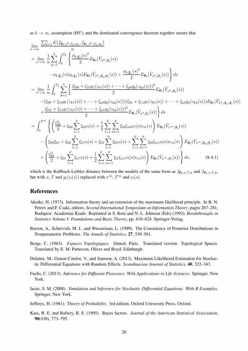
as k → ∞, assumption (H5′), and the dominated convergence theorem together ensure that
limn→∞
∑nk=1K(fθ0,xk,Tk,zk
, fθ1,xk,Tk,zk)
n
= limn→∞
1
n
n∑
k=1
∫ Tk
0
{
φk,ξ0(s)2
2Eθ0(Vxk ,β0
(s))
−φk,ξ0(s)φk,ξ1(s)Eθ0(Vxk,β0,β1(s)) +
φk,ξ1(s)2
2Eθ0(Vxk,β1
(s))
}
ds
= limn→∞
1
n
∫ Tk
0
n∑
k=1
{
(ξ00 + ξ10g1(zk1(s)) + · · ·+ ξp0gp(zkp(s)))2
2Eθ0(Vxk,β0
(s))
−(ξ00 + ξ10g1(zk1(s)) + · · · + ξp0gp(zkp(s)))(ξ01 + ξ11g1(zk1(s)) + · · ·+ ξp1gp(zkp(s)))Eθ0(Vxk,β0,β1(s))
+(ξ01 + ξ11g1(zk1(s)) + · · ·+ ξp1gp(zkp(s)))
2
2Eθ0(Vxk,β1
(s))
}
ds
=
∫ T∞
0
{(
ξ2002
+ ξ00
p∑
l=1
ξl0cl(s) +1
2
p∑
l=1
p∑
m=1
ξl0ξm0cl(s)cm(s)
)
Eθ0(Vx∞,β0(s))
−
(
ξ00ξ01 + ξ00
p∑
l=1
ξl1cl(s) + ξ01
p∑
l=1
ξl0cl(s) +
p∑
l=1
p∑
m=1
ξl0ξm1cl(s)cm(s)
)
Eθ0(Vx∞,β0,β1(s))
+
(
ξ2012
+ ξ01
p∑
l=1
ξl1cl(s) +1
2
p∑
l=1
p∑
m=1
ξl1ξm1cl(s)cm(s)
)
Eθ0(Vx∞,β1(s))
}
ds, (S-4.1)
which is the Kullback-Leibler distance between the models of the same form as fθ0,x,T,z and fθ1,x,T,z,
but with x, T and gl(zl(s)) replaced with x∞, T∞ and cl(s).
References
Akaike, H. (1973). Information theory and an extension of the maximum likelihood principle. In B. N.
Petrov and F. Csaki, editors, Second International Symposium on Information Theory, pages 267–281,
Budapest. Academiai Kiado. Reprinted in S. Kotz and N. L. Johnson (Eds) (1992). Breakthroughs in
Statistics Volume I: Foundations and Basic Theory, pp. 610–624. Springer-Verlag.
Barron, A., Schervish, M. J., and Wasserman, L. (1999). The Consistency of Posterior Distributions in
Nonparametric Problems. The Annals of Statistics, 27, 536–561.
Berge, C. (1963). Espaces Topologiques. Dunod, Paris. Translated version: Topological Spaces.
Translated by E. M. Patterson, Oliver and Boyd, Edinburgh.
Delattre, M., Genon-Catalot, V., and Samson, A. (2013). Maximum Likelihood Estimation for Stochas-
tic Differential Equations with Random Effects. Scandinavian Journal of Statistics, 40, 322–343.
Fuchs, C. (2013). Inference for Diffusion Processes: With Applications in Life Sciences. Springer, New
York.
Iacus, S. M. (2008). Simulation and Inference for Stochastic Differential Equations: With R Examples.
Springer, New York.
Jeffreys, H. (1961). Theory of Probability. 3rd edition. Oxford University Press, Oxford.
Kass, R. E. and Raftery, R. E. (1995). Bayes factors. Journal of the American Statistical Association,
90(430), 773–795.
26

Leander, J., Almquist, J., Ahlstrom, C., Gabrielsson, J., and Jirstrand, M. (2015). Mixed Effects Mod-
eling Using Stochastic Differential Equations: Illustrated by Pharmacokinetic Data of Nicotinic Acid
in Obese Zucker Rats. The AAPS Journal, 17, 586–596.
Liu, J. (2001). Monte Carlo Strategies in Scientific Computing. Springer-Verlag, New York.
Maitra, T. and Bhattacharya, S. (2015). On Bayesian Asymptotics in Stochastic Differential Equa-
tions with Random Effects. Statistics and Probability Letters, 103, 148–159. Also available at
“http://arxiv.org/abs/1407.3971”.
Maitra, T. and Bhattacharya, S. (2016). On Asymptotics Related to Classical Inference in Stochastic
Differential Equations with Random Effects. Statistics and Probability Letters, 110, 278–288. Also
available at “http://arxiv.org/abs/1407.3968”.
Maitra, T. and Bhattacharya, S. (2018a). Asymptotic Theory of Bayes Factor in Stochastic Differential
Equations. Submitted.
Maitra, T. and Bhattacharya, S. (2018b). Asymptotic Theory of Bayes Factor in Stochastic Differential
Equations: Part II. ArXiv Preprint.
Mao, X. (2011). Stochastic Differential Equations and Applications. Woodhead Publishing India Private
Limited, New Delhi, India.
Oravecz, Z., Tuerlinckx, F., and Vandekerckhove, J. (2011). A hierarchical latent stochastic differential
equation model for affective dynamics. Psychological Methods, 16, 468–490.
Overgaard, R. V., Jonsson, N., Tornœ, C. W., and Madsen, H. (2005). Non-Linear Mixed-Effects Mod-
els with Stochastic Differential Equations: Implementation of an Estimation Algorithm. Journal of
Pharmacokinetics and Pharmacodynamics, 32, 85–107.
Robert, C. P. and Casella, G. (2004). Monte Carlo Statistical Methods. Springer-Verlag, New York.
Roberts, G. and Stramer, O. (2001). On Inference for Partially Observed Nonlinear Diffusion Models
Using the Metropolis-hastings Algorithm. Biometrika, 88, 603–621.
Schervish, M. J. (1995). Theory of Statistics. Springer-Verlag, New York.
Schwarz, G. (1978). Estimating the Dimension of a Model. The Annals of Statistics, 6, 461–464.
Sivaganesan, S. and Lingham, R. T. (2002). On the Asymptotic of the Intrinsic and Fractional Bayes
Factors for Testing Some Diffusion Models. Annals of the Institute of Statistical Mathematics, 54,
500–516.
Walker, S. G. (2004). Modern Bayesian Asymptotics. Statistical Science, 19, 111–117.
Walker, S. G., Damien, P., and Lenk, P. (2004). On Priors With a Kullback-Leibler Property. Journal of
the American Statistical Association, 99, 404–408.
27


