
transactions of theamerican mathematical societyVolume 342, Number 2, April 1994
TRANSFER FUNCTIONS OF REGULAR LINEAR SYSTEMS.PART I: CHARACTERIZATIONS OF REGULARITY
GEORGE WEISS
Abstract. We recall the main facts about the representation of regular linear
systems, essentially that they can be described by equations of the form x(t) =
Ax(t) + Bu(t), y(t) = Cx{t) + Du(t), like finite dimensional systems, but now
A, B and C are in general unbounded operators. Regular linear systems are
a subclass of abstract linear systems. We define transfer functions of abstract
linear systems via a generalization of a theorem of Fourés and Segal. We prove
a formula for the transfer function of a regular linear system, which is similar
to the formula in finite dimensions. The main result is a (simple to state but
hard to prove) necessary and sufficient condition for an abstract linear system
to be regular, in terms of its transfer function. Other conditions equivalent
to regularity are also obtained. The main result is a consequence of a new
Tauberian theorem, which is of independent interest.
1. Introduction
In the Hubert space context, an abstract linear system is a linear system whose
input, state and output spaces are Hubert spaces, input and output functions
are locally L2, and on any finite time interval, the final state and the output
function depend continuously on the initial state and the input function. The
concept has been introduced by Salamon [15] to give a unifying framework
for a large class of phenomena usually described as linear, time invariant andwell posed. For the precise definition of this and other concepts used in the
Introduction, see §2.
Regular linear systems are a large subclass of abstract linear systems, probablycomprising every abstract linear system of practical interest. A system is regular
if its output function corresponding to a step input function and zero initial stateis not very discontinuous at zero; the precise requirement is that its average over
[0, t] should have a limit as t —> 0 (see §2). We often prefer to work with
regular linear systems (as opposed to abstract linear systems) because they have
a convenient representation, similar to that of finite dimensional systems, via
equations (1.2) (for the precise statement see Theorem 2.3).
In this paper we investigate the transfer function of regular linear systems.
Received by the editors March 14, 1990 and, in revised form, August 20, 1992.1991 Mathematics Subject Classification. Primary 93C25; Secondary 34G10, 44A10, 47D05.Key words and phrases. Regular linear system, Lebesgue extension, shift-invariant operator,
transfer function, feedthrough operator, Tauberian theorem.
This research was supported partially by the Weizmann Fellowship, and partially by the Air
Force Office of Scientific Research under contract F49620-86-C-0111.
© 1994 American Mathematical Society0002-9947/94 $1.00+ $.25 per page
827
License or copyright restrictions may apply to redistribution; see https://www.ams.org/journal-terms-of-use

828 GEORGE WEISS
We work in the Hubert space context, but in remarks placed at the end of each
section we make it clear which results extend to Banach spaces. Following is an
outline of the paper, including the statement of some of the results.
In §2 we review the necessary background on abstract linear systems and reg-
ular linear systems. For easy reference, the proof of the representation theorem
quoted in this section is given in the Appendix.
In §3 we give a generalization of a theorem of Fourés and Segal [9] concerning
the representation of shift-invariant operators on L2 by transfer functions inH°° . This is needed because the input/output map of an abstract linear system
is a shift invariant operator on LXoc, not on L2 . We define the growth bound yo
of such an operator and prove that a transfer function representation is possible
if and only if yo < oo (this condition is always satisfied by input/output maps
of abstract linear systems).The aim of §4 is to obtain a formula for the transfer function of a regular
linear system. More precisely, we prove the following.
Theorem 1.1. Let Z be a regular linear system with semigroup generator A,
control operator B, observation operator C, and feedthrough operator D. Then
the transfer function Hofl is given for s£C with sufficiently big real part by
(1.1) H(s) = CL(sI-A)-xB + D,
where Cl is the Lebesgue extension of C.
The result has been announced (without proof) in Weiss [18, §4].
The first reaction of the reader to Theorem 1.1 might be to think that this
is obvious. Indeed, we know (see §2) that X is described by the following
equations (which are satisfied for almost every / > 0) :
(1.2a) x(t) = Ax(t) + Bu(t),
(1.2b) y(t) = CLx(t) + Du(t),
where «(•) is the input function, of class LXoc, x(t) is the state at time t,
and y(-) is the output function, again in L20C. Applying formally the Laplace
transformation to ( 1.2), we easily get ( 1.1 ). However, if we think more carefully,
after applying the Laplace integral to equation (1.2b), we have to take Cl outof the integral. But CL (like C) may be a nonclosable operator, so we have to
be careful.There are several ways of proving Theorem 1.1. We prefer to derive it as a
consequence of another theorem which seems to be important in itself. This
theorem gives a rather general answer to the question: when do Cl and the
integral sign commute? It turns out that this is true if Cl is applied to a
function t -* a(t)x(t), where a is scalar and x is a state trajectory of Z, and
both functions do not grow too fast. For details see §4.
In §5 we first prove a new Tauberian theorem about the Laplace transforma-
tion of vector-valued functions of the class IP .
Theorem 1.2. Let W be a Banach space and 1 < p < oo. Suppose v £
Lp([0, oo), W) is such that
(1.3) sup- / ||w((t)||í'í/ct<oo.í>0 t Jo
License or copyright restrictions may apply to redistribution; see https://www.ams.org/journal-terms-of-use

TRANSFER FUNCTIONS OF REGULAR LINEAR SYSTEMS 824
Let v denote the Laplace transform of v . Then, with X positive,
1 r'(1.4) lim- / v(a)da= lim Xv(X),
t^O t Jo A—»oo
i.e., if one of the limits exists, so does the other and they are equal.
We mention that if the limit on the left is known to exist then by a well-
known Abelian theorem (1.4) is true regardless if (1.3) holds. The interesting
case is when only the limit on the right is known to exist. For more details andthe proof see Proposition 5.1, Theorem 5.2, and Remark 5.9.
We need the above result in the proof of the spectral characterization of
regularity, perhaps the main result of the paper, stated below (this is only a partof Theorem 5.8 in §5).
Theorem 1.3. An abstract linear system is regular if and only if its transfer func-
tion has a strong limit at +00 (along the real axis).
With the notation of Theorem 1.1, it is rather easy to prove that for anyelement v in the input space of Z
(1.5) limH(A)v = Z)v,A—»oo
where X is real. Theorem 1.3 shows that conversely, the existence of the limit
in (1.5) implies that Z is regular. (Then it follows that Z has a feedthroughoperator D, and D can be computed by (1.5).)
A simple consequence of Theorem 1.3 is that the cascade connection of two
regular systems is again regular. Maybe the most important consequence of
Theorem 1.3 is that the class of regular linear systems is closed under feedback.
However, we do not discuss cascades or feedback in this paper.
2. Abstract linear systems and regular linear systems: A review
In this section we recall in a very sketchy way some definitions and resultsneeded form other papers. Our aim is not to explain the material or to give
proofs, only to fix the notation, to recall the main points of the theory and toindicate references.
First we introduce some notation. For any Hubert space W and any x >
0, ST will denote the operator of right shift by x on L2([0, 00), W). PT
will denote the projection of L2([0, 00), W) onto L2([0, t], W) (by trun-cation), the latter space being regarded as a subspace of the former. For
u, v £ L2([0, 00), W) and x > 0, the x-concatenation of u and v , denoted
by u o v , is defined by1
UO V = PTM + STV.T
In other words, (uov)(t) = u(t) for t £ [0, t) , while (uov)(t) = v(t-x) for t >T T
x. The shift and projection operators and the operation of concatenation have
natural extensions to L2OC([0, 00), W), and we denote these extensions by the
same symbols. We regard L,2OC([0, 00), W) as a Fréchet space, with the topology
given by the family of seminorms pn(u) — ||P„m||L2 , so that L2([0, 00), W) is
dense in L2OC([0, 00), W).
License or copyright restrictions may apply to redistribution; see https://www.ams.org/journal-terms-of-use

830 GEORGE WEISS
Definition 2.1. Let U, X, and Y be Hubert spaces, fi = L2([0, oo), U) andT = L2([0, oo), Y). An abstract linear system on fi, X, and T is a quadruple
Z = (T,<D,vI,,F),where
(i) T = (T,),>o is a strongly continuous semigroup of bounded linear oper-
ators on X,(ii) O = (®t)t>o is a family of bounded linear operators from fi to I such
that
(2.1) ®x+t(u<>v) = Tt$>xu + <&tV,
for any u, v £Íl and any x, t > 0,(iii) vF=(4'/)i>o is a family of bounded linear operators from X to T such
that
(2.2) Tt+(x = ftxo>P(TIx!
for any x £ X and any x, t > 0, and ¥0 = 0,(iv) F = (Fr),>o is a family of bounded linear operators from fi to T such
that
(2.3) FI+,(MOD)=FIMo(T,Ot« + Fi)j),
for any u, v £Íl and any x, t > 0, and Fo = 0.
U is the input space of Z, X is the state space of Z, and Y is the output
space of Z. The operators 0T are called input maps. The operators *FT are
called output maps. The operators FT are called input/output maps.
Definition 2.1 has been reproduced from Weiss [18]. An equivalent definition
has been given in Salamon [15]. The notation introduced in Definition 2.1 will
be used throughout this section.The intuitive meaning of the operators introduced above is the following:
if x(x) denotes the state of Z at time x > 0, and u £ L2OC[(0, 00), U) and
y e -^ioc([0, 00), T) are the input and output functions of Z respectively, then
(iS)-(ï: î)i%YThe truncated function PTu belongs to the Hubert space L2([0, 00), U), and
similarly for Pry, so that all operators above map Hilbert spaces into Hubert
spaces, as required in the definition.
The simplest example of an abstract linear system is a finite dimensional
system described by the equations
x(t) = Ax(t) + Bu(t), y(t) = Cx(t) + Du(t),
where A, B, C, and D are matrices of appropriate dimensions. In this case,
by a trivial computation
Tx = eM,
<pTu= / eA^-a)Bu(o) do,Jo
(y¥Tx)(t) = CeAtx, forre[0,T),
(¥ru)(t) = C [ eA{t-a)Bu(a) do + Du(t), for t £ [0, t).Jo
For t > x we have (vFTx)(i) = 0 and (FT«)(0 = 0.
License or copyright restrictions may apply to redistribution; see https://www.ams.org/journal-terms-of-use

TRANSFER FUNCTIONS OF REGULAR LINEAR SYSTEMS 831
It is surprising that for any abstract linear system, the operators TT, <PT, and
*FT can be expressed by formulae not much different from the above. For FT
this is true if an additional assumption is made, regularity. Before going intothese matters, we give a more interesting but still very simple example.
Example. We model a delay line as an abstract linear system. Let X = L2[-h,0],
where h > 0, and let T be the left shift semigroup on X with zero enteringfrom the right, i.e., for any x > 0 and Ç £ [-h, 0]
x(C + x), for£ + T<0,
10, for C + x > 0.
Let U = C and for any x > 0 and Ç £ \-h, 0]
w(C + t), for£ + T>0,
L 0, for C + x < 0.
Let Y = C and for any x > 0 and t e [0, t)
{ 0, for t - h > 0.
For / > t we put (<FTx)(f) = 0. Finally, let for any x > 0 and í e [0, t)
^>«>={rA)' í;:¡u-For t > x we put (FTw)(i) = 0. Then Z = (T, O, 4*, F) is an abstract linear
system. For another example worked out in detail the reader may look up
Curtain and Weiss [6].
From the definition of an abstract linear system given above, one can derive
the following two formulae expressing causality:
<DTPT = <DT, FTPT = Ft,
for any x > 0. It is also easy to show that for 0 < x < T
Pt4V = 4\, PTFr = FT.
Let A denote the generator of T. The Hilbert spaces Xx and X_x are
defined as follows: Xx is D(A) with the norm ||jc||i = \\(ßl - A)x\\, where
ß £ p(A) is fixed (this is equivalent with the graph norm), and X_x is the
completion of X with respect to the norm ||x||_i = \\(ßl - A)~xx\\. These
spaces are independent of the choice of ß. If D(A*) is endowed with its
graph norm then X_x can be identified with D(A*)*, the dual of D(A*) withrespect to the scalar product of X. We have Xx cIcLi, densely and with
continuous embeddings. The semigroup T can be restricted to a semigroup
on Xx and extended to a semigroup on X_x. These three semigroups are
isomorphic and we shall denote them by the same symbol (the isomorphism
from X to Xx is (ßI-A)~x and its extension to X-X is the isomorphism from
X_i to X). The generator of T on Xx is the restriction of A to D(A2) and
the generator of T on I_i is the extension of A to X, which is bounded as anoperator from X to X^x. Like in the case of T, we will use the same notation
for the original generator A and for its restriction and extension described
License or copyright restrictions may apply to redistribution; see https://www.ams.org/journal-terms-of-use
832 GEORGE WEISS
above. More information on the spaces Xx and X_ i can be found for example
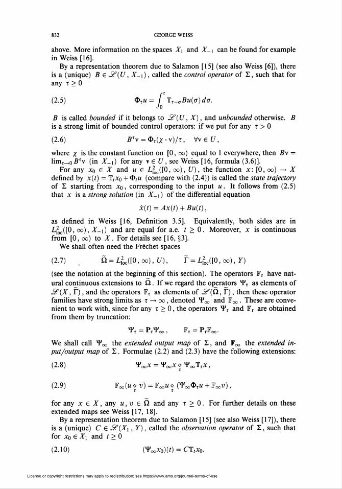
in Weiss [16].By a representation theorem due to Salamon [15] (see also Weiss [6]), there
is a (unique) B £ £f(U, X_x), called the control operator of Z, such that for
any x > 0
(2.5) 4>T«= i Tx_aBu(o)do.Jo
B is called bounded if it belongs to 2f(JJ, X), and unbounded otherwise. B
is a strong limit of bounded control operators: if we put for any x > 0
(2.6) B'y = ^x(x-y)/x, Wet/,
where x is the constant function on [0, oo) equal to 1 everywhere, then Bv =
limT^o#Tv (i° -J^-i) for any v £ U, see Weiss [16, formula (3.6)].
For any Xo £ X and u £ L2OC([0, oo), U), the function x: [0, oo) -» X
defined by x(t) = T,xo + Q>tu (compare with (2.4)) is called the state trajectory
of Z starting from Xo, corresponding to the input u. It follows from (2.5)
that x is a strong solution (in X-X) of the differential equation
x(t) = Ax(t) + Bu(t),
as defined in Weiss [16, Definition 3.5]. Equivalently, both sides are in
L,2OC([0, oo), X-X) and are equal for a.e. t > 0. Moreover, x is continuous
from [0, oo) to X. For details see [16, §3].We shall often need the Fréchet spaces
(2.7) fi = L2OC([0, oo), U), f = L2OC([0,oo),Y)
(see the notation at the beginning of this section). The operators FT have nat-
ural continuous extensions to fi. If we regard the operators *FT as elements of
S?(X, T), and the operators FT as elements of Jz^fi, T), then these operator
families have strong limits as x —► oo, denoted ^^ and F«,. These are conve-
nient to work with, since for any x > 0, the operators *FT and FT are obtained
from them by truncation:
^T = Pr^oo ) FT = PTFoo.
We shall call ^^ the extended output map of Z, and F^ the extended in-
put/output map of Z. Formulae (2.2) and (2.3) have the following extensions:
(2.8) T00x = f00xof00TIx,T
(2.9) Foo(wO V)=¥00UO (YooOrW + FooV),T T
for any x £ X, any u, v £ fi and any x > 0. For further details on these
extended maps see Weiss [17, 18].
By a representation theorem due to Salamon [15] (see also Weiss [17]), there
is a (unique) C £ 2'(XX, Y), called the observation operator of Z, such that
for xo £ Xx and t > 0
(2.10) (^ooXoX/) = CTtx0.
License or copyright restrictions may apply to redistribution; see https://www.ams.org/journal-terms-of-use

TRANSFER FUNCTIONS OF REGULAR LINEAR SYSTEMS 833
C is called bounded if it can be extended continuously to X, and unboundedotherwise. The above formula determines T^ , because Xx is dense in X. A
simple but useful consequence of the above formula is that for any xoel
(2.11) f('¥00xo)(o)da = C [\ax0da.Jo Jo
The Lebesgue extension of C is defined by
i r(2.12) CLJc0 = limC- / Tax0do,
t^0 X Jo
with domain
D(CL) = {x0 £ X\ the limit in (2.12) exists},
which satisfies Xx c D(CL) c X. For any x0 £ X we have that T,x0 £ D(CL)for almost every t > 0 and
(2.13) (4/oox0)(i) = CLT,x0, for a.e. t > 0.
For more information on C¿ see Weiss [17].
For any v e U, the function
is the step response of Z corresponding to v (x was defined after (2.6)).
Definition 2.2. With the notation of Definition 2.1, Z is regular if for any
v e U, the corresponding step response yy has a Lebesgue point at 0, i.e., the
following limit exists (in Y) :
1 fT(2.14) £>v = lim- / ys(o)da.
T-0 X Jo
In that case, the operator D e £?(U, Y) defined by (2.14) is called the feed-through operator of Z.
The above definition has been reproduced from Weiss [18]. The conceptof regular linear system has been vaguely anticipated by Helton [12] in his
definition of "compatible systems" (see also Fuhrmann [10, p. 296]). A class of
abstract linear systems which have received much attention in recent years are
the "Pritchard-Salamon systems" (see Curtain et al. [5] for an updated theory
and references). These systems have continuous step response and so they areregular. The delay line described in the Example is obviously regular, but it is
not a Pritchard-Salamon system.For regular linear systems we have the following representation theorem,
which is the main result of the paper Weiss [18].
Theorem 2.3. Let Z = (T, <P, *F, F) be a regular linear system, with input space
U, state space X and output space Y. Let A be the generator ofT,B the con-
trol operator ofL,C the observation operator ofL, Cl the Lebesgue extension
of C, and D the feedthrough operator of Z.Then for any Xo € X and any u e -£<2OC([0, oo), U), the functions x : [0, oo)
-> X and y £ LX2OC([0, oo), Y) defined by
(2.15a) x(t) = T,xo + Q>tu,
(2.15b) y = x¥00xo + ¥00u,
License or copyright restrictions may apply to redistribution; see https://www.ams.org/journal-terms-of-use
834 GEORGE WEISS
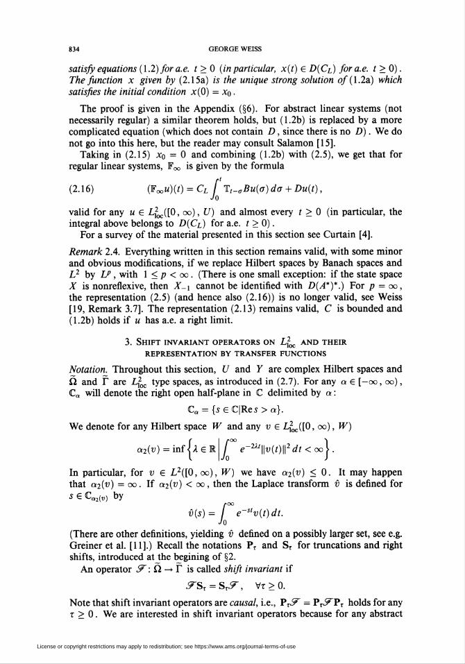
satisfy equations (1.2) for a.e. t > 0 (in particular, x(t) £ D(Cl) for a.e. t > 0).
The function x given by (2.15a) is the unique strong solution of (1.2a) which
satisfies the initial condition x(0) = xq .
The proof is given in the Appendix (§6). For abstract linear systems (not
necessarily regular) a similar theorem holds, but (1.2b) is replaced by a more
complicated equation (which does not contain D, since there is no D). We do
not go into this here, but the reader may consult Salamon [15].
Taking in (2.15) xo — 0 and combining (1.2b) with (2.5), we get that forregular linear systems, Foo is given by the formula
(2.16) (FooW)(0 = CL f Tt-aBu(<j) do + Du(t),Jo
valid for any u £ ¿¿^.([O, oo), U) and almost every t > 0 (in particular, the
integral above belongs to D(Cl) for a.e. t > 0).For a survey of the material presented in this section see Curtain [4].
Remark 2.4. Everything written in this section remains valid, with some minorand obvious modifications, if we replace Hubert spaces by Banach spaces andL2 by LP , with 1 < p < oo . (There is one small exception: if the state space
X is nonreflexive, then X-X cannot be identified with D(A*)*.) For p = oo,
the representation (2.5) (and hence also (2.16)) is no longer valid, see Weiss
[19, Remark 3.7]. The representation (2.13) remains valid, C is bounded and
(1.2b) holds if u has a.e. a right limit.
3. Shift invariant operators on L2oc and their
representation by transfer functions
Notation. Throughout this section, U and Y are complex Hubert spaces and
fi and T are L20C type spaces, as introduced in (2.7). For any a £ [-oo, oo),
Ca will denote the right open half-plane in C delimited by a :
Ca = {s £ C|Res > a}.
We denote for any Hilbert space W and any v £ L]2OC([0, oo), W)
a2(v) = inf ¡X £ RI f°° e-2Xt\\v(t)\\2 dt < oo\ .
In particular, for v £ L2([0, oo), W) we have a2(v) < 0. It may happen
that a2(v) = oo. If a2(v) < oo, then the Laplace transform v is defined for
s £ CQ2(„) by/•OO
v(s)= / e~stv(t)dt.Jo
(There are other definitions, yielding v defined on a possibly larger set, see e.g.Greiner et al. [11].) Recall the notations PT and ST for truncations and rightshifts, introduced atjhe begining of §2.
An operator y : fi —> T is called shift invariant if
yST = STy, Vt>0.
Note that shift invariant operators are causal, i.e., PTy = PTyPT holds for any
x > 0. We are interested in shift invariant operators because for any abstract
License or copyright restrictions may apply to redistribution; see https://www.ams.org/journal-terms-of-use

TRANSFER FUNCTIONS OF REGULAR LINEAR SYSTEMS 835
linear system, the extended input/output map ¥œ is shift invariant. Indeed,
this follows from (2.9) by taking u = 0.We recall the following theorem of Fourés and Segal [9].
Theorem 3.1. Suppose y is a shift invariant bounded linear operator form
L2([0, oo), U) to L2([0, oo), Y). Then there is a unique bounded analytic
S?(U, Y)-valued function H defined on C0 such that for any u e
L2([0, oo), U), denoting y = y m,
(3.1) y(s) = H(s)û(s), Vie C0.
Moreover,
(3.2) sup 11^)11 = 11^11.i€C0
Conversely, any bounded analytic £f(U, Y)-valued function H defined on Co
defines via (3.1) a shift invariant bounded linear operator from L2([0, oo), U)
to L2([0,oo), Y).
For an elementary proof, extensions and references see Weiss [19]. The func-
tion H appearing above is called the transfer function of y.Our goal is to extend Theorem 3.1 for shift invariant continuous operators
from fi to f. First we note that an extension is not always possible: indeed,
consider U = Y = C and y given by
(7«)(i)= / e«-a)1u(o)do.Jo
Then for any u ^ 0 with u(t) > 0, the Laplace transform of Jm is nowhere
defined. For y to be representable by a formula similar to (3.1), we need that
for functions u, y with y = y«, the existence of u should imply the existence
of y. Since we agreed to define û on the half-plane delimited by a2(u),
and similarly for y, this means that a2(u) < oo should imply a2(y) < oo.
Propositions 3.2 and 3.5 give several conditions on y that are equivalent to
the one just stated.We introduce some more notation. For any Hubert space W and any Ael,
the operator ex on L,2OC([0, oo), W) is defined by
(ekv)(t) = ektv(t), Vi>0.
We denote
(3.3) L2([0, oo), W) = exL2([0, oo), W).
Often we omit the argument and simply write L\ . L2 is the same as L\ . L\
is a Hubert space with the norm \v\Li = ||e_^v||L2. It is clear that L\ c L\
for Xx < X2, densely, and a2(u) is the infimum of those X e R for which
U£L\.
Proposition 3.2. Suppose ¡F is a shift invariant continuous linear operator from
fi to T and y e [-oo, oo). Then the following statements are equivalent.
(i) For some x > 0, u£ PTL2 =$ a2(^u) < y.
(ii) For any x > 0, the implication in (i) holds.
(iii) For any u e fi, a2(^u) < max{y, a2(u)} .
(iv) For any X > y, y restricts to a bounded linear operator SF:L\^> L\.
License or copyright restrictions may apply to redistribution; see https://www.ams.org/journal-terms-of-use

836 GEORGE WEISS
Proof. The implications (iv) =>• (iii) =► (ii) => (i) are obvious or very easy. Weclose the loop by proving (i) =$• (iv).
Assume (i) holds and let X > y. Define the continuous linear operator
y:fi^f byy = e.^.
It follows from the simple relation eaSt - eatStea, valid for any real a and
any t > 0, that y is shift invariant. Let e e (0, X - y), then it follows from(i) that y maps PTL2 into Lte ■ By the closed graph theorem, y is bounded
from PTL2 to L2£. Denote for k £ {0, 1,2,...}
&k — (P(A:+1)t - Pfct^Pr-
.5fc may be regarded as an operator from L2 to L2 and as such we estimate its
norm. If we denote by K the norm of yPT as an operator from L2 to L2_e
and take into account that the norm of ~P(k+X)x - P^T, as an operator from L2_E
to L2, is e~kxe, then it follows from the definition that
(3.4) H^ll < Ke~k", Vk£ {0,1,2,...}.
Let v e L2 and w = £Tv . Then v and w can be written in the formoo oo
V = ZZ SJ*VJ ' W = ZZ SkrWk .7=0 k=0
with Vj £ PTL2 and wk £ PXL2 . Indeed, Vj = PxS*jxv , where S* denotes left
shift by t, and similarly for wk . By a simple argument we have
k
SkTWk = ¿Z^k-JVJ>
so the sequence (||tf/t||) is bounded by the convolution of the sequences (||^t||)
and (ll^jl). Let M = \\^\\ + ||y|| + • • • , which is finite according to (3.4).Since ||f 11^,2 = lluo||2 + ||wi||2+-• • , and similarly for w , it follows that ||iü||¿2 <
A/||u||L2, i.e., y is bounded from L2 to L2. Since y = ^_A, y is
bounded from L\ to L\ . D
It is easy to see that the set of numbers y e [-oo, oo) for which the equiv-
alent conditions in Proposition 3.2 are satisfied is either empty or of the form[yo, oo), with y0 £ [-oo, oo).
Definition 3.3. Let y be a shift invariant continuous linear operator from fi to
f. Let yo be the smallest element in [-00,00) for which one (and hence any)
of the conditions in Proposition 3.2 is satisfied. If there are no such numbers
then we put yo = 00. Then y0 is the growth bound of y. We say that y is
exponentially stable if yo < 0.
It is possible to have yo = -00 for nonzero y, for example if y is given by
convolution with a measure having bounded support. In general, y does not
restrict to a bounded linear operator from L2 to L2o. For example, consider
U = Y = C and (7«)(i) = /„' u(a) do . Then y0 = 0, but y does not map L2into itself. We shall see in §4 that if y is the extended input/output map of
License or copyright restrictions may apply to redistribution; see https://www.ams.org/journal-terms-of-use

TRANSFER FUNCTIONS OF REGULAR LINEAR SYSTEMS 837
an abstract linear system, and if a>o is the growth bound of the corresponding
semigroup, then yo < «o •The following lemma is some sort of uniform boundedness principle.
Lemma 3.4. Let W be a Hubert space and ET a continuous linear operator
from W to T. If for any w e W we have a2(£7~w) < oo, then there is a
y £ [-00, oo) such that for any w e W we have a.2(¿Tw) < y.
Proof. Denote for any k, m £N
Vktm = {w£W\\\3rw\\Li<m}.
It is not difficult to see that Vk t m is closed in W. Moreover, the union of all the
sets Vkm is W. By Baire's theorem, there exist y,p£N suchthat Vïtll hasnonempty interior. Then V7<ß- V7ttt contains a ball of radius r > 0 centered
at 0. Since VYtfl - Vïtll c Vy,2li, we get that for any w e W with ||«;|| < r
we have \\¿7~w\\L2 < 2p. Hence, for any w e W we have ||yw||L2 < oo, i.e.,
a2(^w) < y. O
Note. The author is indebted to Hans Zwart for the above short proof.
The number y which we constructed in the proof of Lemma 3.4 is positive,
but of course that does not preclude the possibility of y < 0 or even y = -oo
being a valid choice for some operators y.
Before stating the next proposition we note that if x > 0 and u e PTL2,
then a2(u) = -oo .
Proposition 3.5. Suppose y is a shift invariant continuous linear operator from
fi to T, and let yo be its growth bound. Then the following statements areequivalent.
(i) For some x > 0, u£ PTL2 =*► ol2(SFu) < oo.
(ii) For any u £ fi, a2(u) < oo => a2(5Fu) < oo.
(iii) y0 < oo.
Proof. The implications (iii) => (ii) => (i) are clear (look at (iii) of Proposition
3.2). The implication (i) => (iii) follows from Lemma 3.4, taking W — PXL2(use (i) of Proposition 3.2 to define yo). □
The above proposition shows that a generalization of Theorem 3.1 is con-
ceivable only for operators with growth bound < oo. Now we can state this
generalization.
Theorem 3.6. Suppose SF is a shift invariant continuous linear operator from
fi to f, with growth bound yo < oo. Then there is a unique £?(U, Y)-valued
function H defined on Cyo, which satisfies the following.
(i) H is analytic and for any y > yo it is bounded on Cy, more precisely
(3-5) sup ||H(s)|| = 1^11^,2,^.sec, ^ y j>
(ii) If u £ fi with a2(u) < oo, then denoting y = ¡Fu and c*o =
max{yo, a2(u)}, we have
(3.6) y(s) = H(s) ■ û(s), VS e Cao.
License or copyright restrictions may apply to redistribution; see https://www.ams.org/journal-terms-of-use

838 GEORGE WEISS
Conversely, suppose H is an <S?(U, Y)-valued function on Cyi, where yx e
[-00,00). If H is analytic and for any y > yx, it is bounded on Cy, then H
defines via (3.6) a shift invariant continuous linear operator from fi to t, with
growth bound yo < yx (in particular, H has an extension to Cyo with properties
(i) and (ii) above).
Proof. Let y and yo be as in the first part of the theorem. For any y > yo,
put y, = e-7!Fey, so ZFy is shift invariant (see the beginning of the proof of
Proposition 3.2). By (iv) of Proposition 3.2, y is bounded from L2 to L2,
so y^ is bounded from L2 to L2. Moreover, since ey is a norm preserving
transformation from L2 to L2 , we have
(3-7) 11^1^,^ = 11^1^,^).By Theorem 3.1 there is a unique bounded analytic ^f(U, V")-valued function
Gy on Co, representing y, like in (3.1). Coming back to y, we get that for
any u e L2, (3.6) holds with Hy(s) = Gy(s - y) in place of H(s). Moreover,
by (3.2) and (3.7) we get that (3.5) holds in Hy in place of H.Let (y„) be a decreasing sequence in (yo, 00) such that y« -> yo. Hy„ is
defined on Cn , and it is analytic and bounded there. Since L2n+1 c L2n densely,
Hj,n is uniquely determined by the restriction of y to L2n+i, which implies
that H.7n is the restriction of H>,n+1 to Cyn. This makes it possible to define by
induction an analytic function H on Cj,0 such that for any n e N, Hïn is a
restriction of H. It follows that for any y > yo , Hy is the restriction of H to
Cy, so (i) and (ii) are satisfied.Conversely, let H and yx be as in the second part of the theorem. Let
y > yx and G(s) - H(s + y). Then by the second part of Theorem 3.1, G
defines via (3.1) a shift invariant bounded linear operator y from L2 to L2 .
Put y = eyETe-y, so y is shift invariant and bounded from L2 to L2 , and
for u £ L2 it satisfies (3.6) on Cy. Obviously y extends to a shift invariant
continuous operator from fi to f and its growth bound yo < y. This being
true for any y > yx, we get yo < yi ■ □
Definition 3.7. When y and H are as in the first part of the above theorem,
then H is called the transfer function of y .
Remark 3.8. Almost everything written in this section remains valid, after some
simple and obvious modifications, if we replace Hubert spaces by Banach spaces
and L2 by IP , with 1 < p < 00 (in particular, the notation cx2(v) should be
replaced by ap(v)). The exceptions are the following: in (3.2) and (3.5), the
sign = has to be replaced by < , and the converse (last) parts of both Theorems
3.1 and 3.6 will no longer hold. This is because the converse part of Theorem 3.1
is a consequence of the Paley-Wiener theorem, which has no correspondent forBanach spaces. The proof of the first part of Theorem 3.1 for Banach spaces
and Lp can be found in Weiss [19]. For p — 00, nothing remains true of
Theorem 3.1, see Weiss [19] (Propositions 3.2 and 3.5 and Lemma 3.4 can be
extended also for this case).
4. When can we take Cl out of an integral,and the formula for the transfer function
Recall that the growth bound of a strongly continuous semigroup T is the
smallest element &>o £ [-00, 00) such that for any œ > ojo, there is an Mm > 1
License or copyright restrictions may apply to redistribution; see https://www.ams.org/journal-terms-of-use

TRANSFER FUNCTIONS OF REGULAR LINEAR SYSTEMS 839
for which
(4.1) ||T,|| < Afa,^0", V*>0.
In particular, T is exponentially stable if coo < 0.
As mentioned at the beginning of §3, the extended input/output map of any
abstract linear system is a shift invariant continuous operator. We start by a
simple proposition relating the growth bound of this operator (see Definition
3.3) with the growth bound of the semigroup. This proposition is due to Sala-mon [15, Lemma 2.1] but for greater clarity we also give a proof.
Proposition 4.1. Let Z = (T, O, *F, F) be an abstract linear system. Denote by
a>o of the growth bound of T and by y0 the growth bound of Foo • Then
Yo < Mo-
Proof. First we prove that
(4.2) a2(xP0oXo)<a)0, Vx0 e X
(the notation a2(v) was introduced at the beginning of §3). We have for any
X £ R and any n e N
ll^^olli.2 = I X/\k=0
(proof by induction using (2.2)). It follows that
\\VnXo\\q<M\Te-2k*\\Tk\\2\ Uxoll,
where M is the norm of *Fi as an operator from X to L\ . Now let us assume
that X > Wo and let to e (too, X). Using the last inequality together with (4.1),
we get that the operators ¥„ form X to L\ are uniformly bounded. Since
¥„ = Pn^oo , it follows that ^oo is bounded from X to L\ . This being true
for any X > too, we have proved (4.2).
Choose x > 0. For any u £ PXL2, (2.9) implies
W00u = Wxuoy¥00<&xu.x
Taking xo = <&xu in (4.2), it follows that a2(¥00u) < too. Using (i) of Propo-
sition 3.2 to define yo, we get yo < too . o
It follows from Proposition 4.1, together with Theorem 3.6, that Foo can be
represented by means of a transfer function (defined on Cyo). By the transfer
function of Z we simply mean the transfer function of F«,. The main aim
of this section is to prove formula (1.1) expressing the transfer function of a
regular linear system in terms of the operators appearing in the representation
(1.2) (see Theorem 4.7). As noted in the Introduction, we prove this formula
using a theorem concerning integrals containing C/_ (Theorem 4.6), which is
of independent interest.
Remark 4.2. In Salamon [14, 15] and in Curtain and Weiss [6], the transfer
function H of an abstract linear system was introduced in a different way,
License or copyright restrictions may apply to redistribution; see https://www.ams.org/journal-terms-of-use

840 GEORGE WEISS
leading to H being defined on p(A) (the resolvent set of the generator). I think
that this is not natural, because the transfer function should depend only on the
input/output map, and not on any particular state space realization attached to
it. However, the transfer functions defined in these two approaches are equal
on the half-plane CWo, so that they determine the same input/output maps.
Remark 4.3. An immediate consequence of Proposition 4.1 is that exponential
stability of T (too < 0) implies exponential stability of F^ (yo < 0). Severalauthors have investigated the following problem: under which additional as-
sumptions on Z does the converse implication hold. Clearly this is equivalent
to asking when yo = too holds. We refer to Curtain [3], Curtain et al. [5, §5]
and, for the most general results currently available, to Rebarber [13].
Notation. For the rest of this section we shall work with regular linear systems,
using the notation introduced in (2.7), Theorem 2.3, and (3.3). This means that
the symbols U, X, Y (Hubert spaces), fi, f, L2W (function spaces), Z, T, O,*F, F (regular linear system and its operator families) and A, B, C, Cl, D
(operators representing the system via (1.2)) need to further explanation, too
and yo will be as in Proposition 4.1 (growth bounds). PT and ST will denote
truncations and right shifts (see the beginning of §2). S* will denote the oper-
ator of left shift by x > 0 on both fi and F (the restriction of S* to L2 is
the adjoint of the restriction of ST to L2).For any x > 0, the operator C[ e ¿ï?(X, Y) is defined by
(4.3) Clz = C-\\aT Jo
zdo.
It is clear from the definition that for any z e D(Cl) , limT_o CLz = Clz .
It is an immediate consequence of Theorem 2.3 that if x is a state trajectoryof Z (see §2), then limr_o CTLx(t) = Clx(í) for a.e. t > 0. We prove that the
convergence is valid also in another sense.
Lemma 4.4. Let to > to0 and u £ £-¿([0, oo), U). Let x be a state trajectory
o/Z corresponding to the input u. Then for Cl defined as in (4.3) we have
lim Clx = CLx in Z¿([0, oo), Y).T—»0
Proof. Let / denote the constant function on [0, oo) equal to 1 everywhere.
We define for every x > 0 the operator Dx e ¿2?(U, Y) by
DTv=UT((4.4) &v = - (Foo(;rv))((7)¿ff
By (2.14), limT_o.DTv = Dv, so by the uniform boundedness principle the
operators Dx are uniformly bounded for x e (0, 1]. It follows by the Lebesgue
dominated convergence theorem that
(4.5) lim DTu = Du in £2.
Let us derive a useful identity. Clearly for any q, r e T and any t > 0,S*(qo r) = r. Applying this to (2.8) and (2.9), we get that for any z e X and
any /, gefi,
S( ToqZ = TooTfZ ,
License or copyright restrictions may apply to redistribution; see https://www.ams.org/journal-terms-of-use

TRANSFER FUNCTIONS OF REGULAR LINEAR SYSTEMS 841
s;f00(/oj) = «p00<d//+f0oí.
Adding these equalities and using that / = fe S*f, we get an identity which
expresses the fact that the system Z is time-invariant:
S;pFooZ + Foo/) = ^oo(Ttz + <t>tf) + FooS;/.
Now we consider the state trajectory x . We put Xo = x(0), then x is given
by (2.15a). Let y be defined by (2.15b) (the output function), so by Proposition4.1 and by (4.2) we have y e £2 . Taking in the last identity z = Xo and f —u,we get that for any t > 0
(4.6) S¡y = 1¥00x(t) + ¥00S*u.
We consider that u(t) is well defined for every t > 0, i.e., we make a choice
from the equivalence class of functions equal a.e. which represent u. Let for
any t > 0 the function e, e fi be defined by
(4.7) s,(o) = u(t + o) - u(t),
so S*m = x • u(t) + et. Substituting this into (4.6) and then integrating on [0, t]we get, using (2.11)
/ y(t + o)do = C I Tax(t)do+ [ (¥00(x -u(t)))(o)doJo Jo Jo
+ [ (¥aoe,)(o)do.Jo
Dividing everything by x and using (4.3) and (4.4) we get
(4.8) - [ y(t + o) do = CTLx(t) + Dzu(t) + - f (V^e^o) do.t Jo Wo
We mention that this formula is needed also in the proof of the representation
theorem (Theorem 2.3), as given in the Appendix.
It is easy to see that in the space £2 we have limT_+0(l/i') $ly(t + o)do =y(t) (both sides are defined for a.e. t > 0). Using the representation of y given
in Theorem 2.3, this becomes
lim IfT-0 T Jo
(4.9) lim-/ y(t + o)do = CLx(t) + Du(t) in L
(both sides have to be regarded as functions of t, defined for a.e. t > 0). If
we can prove that
(4.10) lim- / (Fooet)(iT)rfff = 0 in L2Wt-»0 X Jo
(again, both sides are functions of t), then (4.5), (4.8), (4.9), and (4.10) implythe conclusion of the lemma. So it remains to prove (4.10).
We have for x e (0, 1], using that PTFoo = FT and ||FT|| < ||Fi||,
I11 rz 1 fT ( \ tx \ xl2-/ (FooCtXff)*/* <-/ \\(¥xet)(o)\\do<(U ||(FTei)(tf)ll2^
II wo x Jo \T Jo J
<l|Fill(I/T|M^)ll2^X
License or copyright restrictions may apply to redistribution; see https://www.ams.org/journal-terms-of-use

842 GEORGE WEISS
Both sides above are in £¿ , when regarded as functions of t e [0, oo). Using
Fubini's theorem we get
I\ f (Foo^X*)do < ||F,||2 [°°e~2M (- f \\et(o)\\2do] dtII WO Li JO \T JO J
= \Wif- f re-2(ût\\st(o)\\2dtdoi Jo Jo
= \\¥xf-\X\\&au-ufLldo.X Jo M
Since (SJ)a>o is a strongly continuous semigroup on £2 , it follows that the
last expression on the right-hand side above tends to zero as x —► 0, i.e., we
have proved (4.10). D
Remark 4.5. Let x be a state trajectory of Z corresponding to an input u e fi
and let C\ be defined as in (4.3).Then
lim CJx — ClX in f.T^O L
To prove this, we have to show that PrQx —► PrQ,x in £2, for any
T > 0. So let T > 0 and let xj be the state trajectory starting from x(0),
corresponding to the input Pr" • By causality (see the beginning of §3) we have
PrCpc = Pj-C¿x:r, and similarly for Cl in place of C[ . Let to > too. Since
P7-W e L2W , Lemma 4.4 implies that P^C^x -> PrC¿x in £2 as x —» 0, which
is equivalent to convergence in £2.
Theorem 4.6. Let to > too and u e £¿([0, 00), U). Let x be a state trajectory
of Z corresponding to the input u, and let a e £2_(U[0, 00). Then(•OO /.OO
(4.11) / CLa(t)x(t)dt = CL I a(t)x(t)dtJo Jo
(in particular, /0°° a(t)x(t) dt £ D(CL)).
Proof. The operators C\(x > 0) were defined in (4.3). It is easy to verify that
the functions x, C\x and C^x are in £2 (use Proposition 3.2 for x andC\x and Proposition 4.1 and (4.2) for Q,x). It follows that the functions ax,
C\oi.x and Q,ax are in £' and, by Lemma 4.4,
lim C\ax — Clolx in £'([0, 00), Y).T—»0
Since C[ commutes with the integral sign, we geti*00 /»oo
/ CLa(t)x(t)dt = lim Cl a(t)x(t)dt.Jo T-° Jo
By the definition of CL (see (2.12)), this implies that /0°° a(t)x(t) dt e D(CL)and (4.11) holds. D
We mention that a weaker version of Theorem 4.6, valid for Pritchard-
Salamon systems and finite dimensional U, was given in [5, §3].
We restate Theorem 1.1 in a somewhat more precise way. Remember that
we are still using the notation introduced before Lemma 4.4. Now, all Hubert
spaces are assumed to be complex.
License or copyright restrictions may apply to redistribution; see https://www.ams.org/journal-terms-of-use
TRANSFER FUNCTIONS OF REGULAR LINEAR SYSTEMS 843
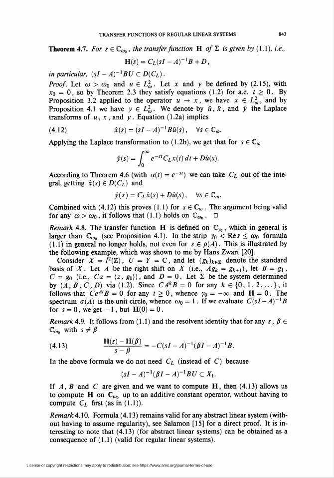
Theorem 4.7. For s e C^, the transfer function H of Z is given fry (1.1), i.e.,
H(s) = Cl(sI-A)~xB + D,
in particular, (si - A)~XBU c £>(C¿).
Proof. Let to > to0 and u £ L2». Let x and y be defined by (2.15), withXo = 0, so by Theorem 2.3 they satisfy equations (1.2) for a.e. t > 0. By
Proposition 3.2 applied to the operator u —* x, we have x e £2 , and by
Proposition 4.1 we have y £ £¿. We denote by û, x, and y the Laplace
transforms of u, x, and y . Equation (1.2a) implies
(4.12) x(s) = (si - A)'xBû(s), VseCo,.
Applying the Laplace transformation to (1.2b), we get that for ieCw
/•OO
y(s)= e-stCLx(t)dt + Dû(s).Jo
According to Theorem 4.6 (with a(t) = e~st) we can take Cl out of the inte-
gral, getting x(s) e D(Cl) and
y(x) = CLx(s) + Du(s), Vs e Cw.
Combined with (4.12) this proves (1.1) for s e Cw . The argument being valid
for any to > too , it follows that (1.1) holds on CWo. D
Remark 4.8. The transfer function H is defined on Cyo, which in general is
larger than C<u0 (see Proposition 4.1). In the strip y0 < Res < to0 formula
(1.1) in general no longer holds, not even for 5 e p(A). This is illustrated by
the following example, which was shown to me by Hans Zwart [20].
Consider X = /2(Z), U = Y = C, and let (gk)k€z denote the standard
basis of X. Let A be the right shift on X (i.e., Agk = gk+x), let B — gx,C = go (i.e., Cz = {z, go)), and D = 0. Let Z be the system determined
by (A,B, C, D) via (1.2). Since CAkB = 0 for any k e {0, 1, 2, ...}, itfollows that CeAtB = 0 for any t > 0, whence yo = -oo and H = 0. Thespectrum o(A) is the unit circle, whence too = 1. If we evaluate C(sI-A)~xB
for s = 0, we get -1, but H(0) = 0.
Remark 4.9. It follows from (1.1) and the resolvent identity that for any s, ß £
C^ with í # ß
(4.13) H(a) - H(l) = _C{sI _ A)_X{ßI _ A)_lßs p
In the above formula we do not need C¿ (instead of C) because
(si - A)~x(ßl - A)~XBU c X\.
If A, B and C are given and we want to compute H, then (4.13) allows us
to compute H on Co,,, up to an additive constant operator, without having to
compute CL first (as in (1.1)).
Remark 4.10. Formula (4.13) remains valid for any abstract linear system (with-
out having to assume regularity), see Salamon [15] for a direct proof. It is in-teresting to note that (4.13) (for abstract linear systems) can be obtained as a
consequence of (1.1) (valid for regular linear systems).
License or copyright restrictions may apply to redistribution; see https://www.ams.org/journal-terms-of-use

844 GEORGE WEISS
We sketch the proof. Let Z be an abstract linear system and let Zc be the
system obtained by the cascade connection of Z followed by an integrator.Clearly Zc has continuous step responses, so that it is regular. If H and Hc
are the transfer functions of Z and Zc, then Hc(s) = (l/s)H(s). The state
space of Zc is 1x7, where X and Y are the state and output spaces of Z.
If A and C are the semigroup generator and observation operator of Z, then
the corresponding operators for Zc are
AC={Ac o)' cc = (° ^
with D(AC) = D(A) x Y. Let B and Bc denote the control operators of Z and
Zc (it seems that there is no simple way to express Bc in terms of A, B, C).
Then by (1.1), W(s) = Cc(sl - AC)~XBC. We can get B and Bc as strong
limits, for x —> 0, of Bx and Bcx, which are families of bounded control
operators, see (2.6). Moreover, the first component of Bcx is exactly Bx. If
we denote HCT(s) = Cc(sl - AC)~XBCX, then (by an elementary computation)
sWx(s)-ßWx(ß) = C[(sl - A)'1 - (ßl - A)~X]BX. Applying both sides to any
fixed element of the input space, taking limits as x —> 0 and using the resolvent
identity, we get (4.13).
Remark 4.11. Abstract boundary control systems, as introduced in Salamon [ 14,
§2.2], are abstract linear systems with B injective and such that XnBU — {0} .
Salamon proved that such systems have a relatively simple representation in
terms of a differential and two algebraic equations, valid for smooth inputs
and compatible initial conditions (see [14]). Part of his construction is the
introduction of the Hilbert space Z = {z e X\Az e X + BU} and of theoperators T e &(Z , U) and K e S?(Z, Y) such that (A + BT)z e X for any
z £Z (this determines Y) and
H(s) = K(sI-A)~xB, VseCV
It is somewhat confusing that both Cl and K are extensions of C and ap-pear in formulae expressing H, but otherwise have little in common. However,
for regular boundary control systems we have Z c £>(Q.) and the relationship
between the restriction of Cl to Z and K is simple:
Kz = (cl + dt)z, ^z£Z
(this follows by a short computation).
Remark 4.12. Everything in this section remains valid, with minor and obvious
modifications, if we replace Hilbert spaces by Banach spaces and £2 by LP ,
with 1 < p < oo (in Theorem 4.6 we have to assume a e ^„[O, oo), where
l/P + l/q = 1) • For p = oo, only Proposition 4.1 remains valid.
5. A Tauberian theorem about the Laplace transformation
on £2 , and the spectral characterization of regularity
First a few words on terminology, following Doetsch [8]. Let y be a function
on [0, oo ), which has a Laplace transform y. A theorem which tells something
about the asymptotic behavior of y, based on the asymptotic behavior of y ,
is called an Abelian theorem. Usually, the converse of an Abelian theorem is
not true, unless we impose an additional condition on y, called a Tauberian
License or copyright restrictions may apply to redistribution; see https://www.ams.org/journal-terms-of-use

TRANSFER FUNCTIONS OF REGULAR LINEAR SYSTEMS 845
condition. Such a partial converse is called a Tauberian theorem. There is latelya renewed interest in Tauberian theory, see, for example, Arendt and Priiss [1],
Batty [2], and the references therein.
Now we are interested in functions that belong to £2([0, oo), Y), where Y
is a Hilbert space (for Banach spaces see Remark 5.9). First we state a simpleAbelian theorem (see Doetsch [8, p. 473] for the scalar version).
Proposition 5.1. Let y e £2([0, oo), Y) be such that for t e (0, oo)
(5.1) lim- f y(o)do = d.t-*o t Jo
Then for X e (0, oo)
(5.2)
Proof. For any t > 0
(5.2) lim Xy(X) = d.X—»oo
/ y(o)do = td + te(t),Jo
where e is a continuous and bounded 7-valued function on (0, oo), with
||e(i)|| -> 0 for t -> 0. Applying the Laplace transformation, we get for X > 0
i i r°°jy(X) = j2-d + J e-kttz(t)dt,
whence/■OO
\\Xy(X) - d\\ < X2 e-xtt\\e(t)\\dt.Jo
It is an easy exercise to show that the right-hand side above tends to zero as
X -» oo . (Hint: decompose like /0°° = jQT + /r°° , with x = 1/vX) D
The following partial converse of Proposition 5.1 is known (see Doetsch [8,
p. 512]): if Y - R and the Tauberian condition limsup(^0.K0 < °° (°rliminf._0};(0 > ~°°) holds, then (5.2) implies (5.1).
We shall prove another partial converse of Proposition 5.1 (our Tauberiancondition is (5.3)).
Theorem 5.2. Suppose y e £2([0, oo), Y) is such that
(5.3) sup) / ||y(<7)||2¿<x<oc.í>0 f Jo
If the Laplace transform y satisfies (5.2), then y satisfies (5.1).
Proof. Let us denote the left-hand side of (5.3) by M2. First we prove that/•oo
(5.4) X e-u\\y(t)\\dt<M, VA > 0.Jo
Indeed, we have for any X > 0
/•OO /-OO / ft \
Xjo e-*'\\y(t)\\dt = X2J e~lt (J \\y(o)\\doj dt
<^¡^~^{jJ^\\y((T)\\2d(^ dti»00
< MX2 / e~Xttdt = M.Jo
License or copyright restrictions may apply to redistribution; see https://www.ams.org/journal-terms-of-use

846 GEORGE WEISS
The next step is to show that for any continuous function /: [0, 1] —► R we
have/•OO fOO
(5.5) lim X e-x,f(e-Xt)y(t)dt = d e~tf(e-t)dt.A—oo J0 Jo
We have
f°° 1lim X / e-Xt(e-u)ny(t) dt =-r lim X(n + l)y(X(n + 1))
A—>oo Jo n + \ X—»oo
i r°°= —!—d = d e-^e-'fdt,
n+l Jo '
which implies that (5.5) is true for any polynomial /. We denote for any
bounded, measurable g: [0, 1] -> R and any X > 0/»OO
(5.6) E(X,g) = X e-klg(e-xt)y(t)dt.Jo
Let /: [0, 1] -> R be continuous and let (f„) be a sequence of polynomials
such that fn-*f uniformly. Then (5.4) implies
\\E(X
/•OO
, /„) - E(X, f)\\ < X / e-xt\fn(e~lt) - f(e~Xt)\ • \\y(t)\\ dtJo
<M SUP \fn(x)~f(x)\,xe\o,\]
so E(X, fn) -> E(X, f) uniformly with respect to X. Therefore
lim E(X, f) - lim lim E(X, fn),A-»oo n-»ooA-»oo
which is the same as (5.5).The next step is to prove (5.5) for / replaced by a particular discontinuous
function fo : [0, 1] —> K, defined by
J 0, forxefO,*?-1),
MX) I 1/x, forx£[e-x, 1].
We approximate y¿ by a family of continuous functions fe, s > 0, de-
fined as follows: f(x) = fo(x) for any x in [0,1] except in the subinterval
[e~x~c, e~x), and fe interpolates linearly inside this subinterval, i.e.,
-l-E
/«(*)= It \-,_f -g. forxefe-1-8,^-1).
It is elementary to check that for any í, 2 > 0
g-Aí|/£(g-A') - /o(g-A')l < Z[l/A, lM(l+£)](0 ,
where ^j denotes the indicator function of the interval J. We have, using the
above inequality,
\\E(X,f£)-E(X,fo)\\<X \W)\\dtJi/x
<Ve[x \\y(t)\\2dt
License or copyright restrictions may apply to redistribution; see https://www.ams.org/journal-terms-of-use

TRANSFER FUNCTIONS OF REGULAR LINEAR SYSTEMS 847
Assuming for convenience e < 1 and denoting 2/X = x, we get by (5.3)
\\E(X, f) - E(X, fo)\\ <V2i(^f \\y(t)\\2 dt^j <VTs-M,
which shows that E(X, fE) -* E(X, fo) uniformly with respect to X. Therefore
lim E(X, fo) = lim lim E(X, fi).A—»OO £—»OA—»oo
Since (5.5) holds for fe in place of /, we have now obtained that it also holds
for fo in place of /, i.e.,
ri/x ,1lim X / y(t)dt = d / dt,»-*°° Jo Jo
'l/X
im X IA-'oo Jo
which is exactly (5.1). D
Problem 5.3. I was not able to construct a function y e £2[0, oo) satisfying
(5.2) but not (5.1). Such a function would show that the Tauberian condition
(5.3) cannot be omitted in Theorem 5.2. For any p e [1, 2), we can construct
such a counterexample in £/[0, oo), as follows:
Let /: [0, oo) -* R be defined by
and put
where
r sin27ti for t£ [0,1],
1/(0 10 fori>l,
y(t) = Yik2lpgkf(k(k+l)t-k),k=\
l/n2 forÂ: = 2\ «egk -{
By some standard computations which we do not display here, y e LP[Q, 00),(5.2) holds with d = 0, but the limit in (5.1) does not exist.
It would be a very interesting result, if it could be proved, that for p > 2 we
do not need (5.3) in Theorem 5.2 (see also Remarks 5.7 and 5.9).
The following proposition is a strengthening of Proposition 5.1. Recall the
notation 0.2(y), defined in §3. We introduce a notation for angular domains in
C : for any y/ e (0, n]
(5.7) 2T(,i0 = {We(0,oo), <t> e (-¥,¥)}■
Proposition 5.4. Suppose y e £,2OC([0, 00), Y) is such that e*2(y) < 00 and (5.1)
holds. Then for any y/ e (0, n/2)
(5.8) lim sy(s) = d.se2r(v),|s|-»oo
Proof. This can be obtained by slightly modifying the proof of Proposition 5.1.
Now the function e will not be bounded in general, but it can be written in
the form e(t) = eo(t)eat, where £0 is bounded and a > a2(y). The variable
X > 0 has to be replaced with 5 (and sometimes with |s|), where 5 e ^(y)
and Re s > a . O
License or copyright restrictions may apply to redistribution; see https://www.ams.org/journal-terms-of-use

84Í GEORGE WEISS
We cannot allow y/ = n/2 in (5.8), as the simple example y (s) = e~s/(s+ 1)
shows. We did not state Proposition 5.1 in this strengthened form from the
beginning, because this would have obscured its relationship to Theorem 5.2.
The following corollary is a strengthening of Theorem 5.2.
Corollary 5.5. Suppose y £ £i2oc([0, oo), Y) is such that a2(y) < oo and
1 /"'(5.9) lim sup - / ||y((T)||26?(T<oo.
f->0 t Jo
If the Laplace transform y satisfies (5.2), then y satisfies (5.1).
Proof. Decompose y = yx +y2, where yx is supported on [0, 1] and y2 on
[1, 00). By Proposition 5.4, lim^ooAy^A) = 0. It follows that lim^_ooÂPiW= d , and (5.9) implies that yx also satisfies (5.3). By Theorem 5.2 we get that
yi satisfies (5.1), i.e., y satisfies (5.1). □
We return now to systems theory.
Definition 5.6. Let Z be an abstract linear system, with state space X, semi-
group generator A and observation operator C. We define the operator C¿
by
(5.10) CLx0= lim CX(XI-A)-xx0,X—»+oo
where X e R, with domain
D(CL) = {xo £ X\ the limit in (5.10) exists}.
Remark 5.7. Denoting by Cl the Lebesgue extension of C (see (2.12)), we
have that Cl is an extension of C¿ , i.e.,
(5U) D(CL)CD(CL)CX,CLx = CLx, VxeZ)(CL).
This follows from Proposition 5.4 with y(t) = ¥00*o, where ¥00 is the ex-
tended output map of Z (see §2), using (2.11) and (4.2). (A direct proof was
given in Weiss [17, Proposition 4.7], but without defining C¿.)
I do not know if the first inclusion in (5.11) can be strict. In order to answer
this question, a solution of Problem 5.3 would be needed. In any case, we will
see below that for any practical purpose C¿ and Cl are interchangeable, we
can always use the one which suits us better.
The following theorem contains Theorem 1.3.
Theorem 5.8. Let Z = (T, O, *F, F) be an abstract linear system, with input
space U, state space X, output space Y, semigroup generator A, control op-
erator B, observation operator C, and transfer function H. The operators Cl
and Cl are defined in (2.12) and (5.10), and too is the growth bound of T.Then the following statements are equivalent.
(1) Z is regular, i.e., for any v e U the limit in (2.14) exists.
(2) For any s e p(A) we have that (si - A)~XBU c D(CL) andCL(sI - A)~XB is an analytic J¿?(U, Y)-valued function of s on p(A),
bounded on any half-plane Cw with to > to0 .
License or copyright restrictions may apply to redistribution; see https://www.ams.org/journal-terms-of-use

TRANSFER FUNCTIONS OF REGULAR LINEAR SYSTEMS 849
(3) There exists s e p(A) such that (si - A)~XBU c D(CL) ■
(4) There exists s e p(A) such that (si - A)-XBU C D(CL) ■(5) Any state trajectory of Z is a.e. in D(Cl) ■
(6) Any state trajectory of Z is a.e. in D(Cl) ■
(7) For any v e U and any y/ e (0, n/2), H(s)v has a limit as \s\ —► oo
in W(yi) (see (5.1)).(8) For any vet/, H(A)v has a limit as X —» -foe in R.
Moreover, if the limits mentioned in (I), (1), and (8) above exist, then they
are equal to Dv, where D is the feedthrough operator ofL.
Proof. Our plan is to prove the implications in the following diagram
(5) => (6)
(1) ==> (2) => (3) => (4) =M8)
(7)
This will show that (1) implies any other point and any other point implies (8).
Then, we will close the loop by proving that (8) implies (1) (it is here that we
need the Tauberian theorem proved earlier).
The implication (1) => (2) : Suppose (1) holds. Theorem 4.7 implies that for
s e Cœo we have (si - A)~XBU C D(CL) and CL(sI - A)~XB e S?(U, Y).By the resolvent identity we obtain that these properties remain true for any
s e p(A) and the function G defined on p(A) by G(s) = Cl(sI - A)~XBsatisfies (4.13) for any s, ß £ p(A) with s / ß. It is easy to show (using
again the resolvent identity) that C(sl - A)~x is an analytic Sf(X, Y~)-valued
function of s on p(A). Now (4.13) (with G in place of H) implies that also
G is analytic on p(A). It remains to show the boundedness of G on certain
half-planes. By Theorem 4.7 we have G(s) - H(s) - D for s e C^. ByTheorem 3.6 and Proposition 4.1, H is bounded on Cw for any to > too, so
the same applies to G.
The implication (2) => (3) is trivial.The implication (3) => (4) follows from (5.11).The implication (4) =► (8) : Suppose (4) holds. By the resolvent identity
we get that (si - A)~XBU c D(CL) for any 5 € p(A). We denote, for any
s £ p(A), G(s) = CL(sI -A)~XB, which by (5.10) means that for any v e U
(5.12) lim CX(XI - A)~x(sl - A)~xBy = G(s)\.A—»oo
Since for any z e X, lim/l_>00(A/ - A)~xz = 0 in Xx and C is bounded on
Xx, it follows that for any 5 e p(A) and any v e U
lim Cs(XI-A)-x(sI-A)~xBv = 0.A—»oo
Subtracting this side by side from (5.12) and using the resolvent identity, we
get that limA^oo[G(5) - G(A)]v = G(s)v, which shows that
(5.13) limG(A)v = 0, Wei/.A—»oo
License or copyright restrictions may apply to redistribution; see https://www.ams.org/journal-terms-of-use

850 GEORGE WEISS
By the resolvent identity, G(s) satisfies (4.13) for any s, ß e p(A) with s ^ ß .
By Remark 4.10, H satisfies (4.13) for any s, ß e C^ with 5 ̂ ß . It follows
that for 5 e C<b0 , H(s) - G(s) is independent of s . This, together with (5.13)implies (8).
The implication (1) => (5) is contained in Theorem 2.3.
The implication (5) => (6) follows from (5.11).The implication (6) =>■ (4) : Let s £ p(A) and v e U and denote Xo =
(si - A)~XB\. Then the state trajectory of Z starting from Xo , corresponding
to the input u(t) — estv, is given by x(t) = es'xo (indeed, it is clear that these
functions satisfy (1.2a)). If (6) holds then this implies x0 e D(CL) ■ Since thechoice of v e U was arbitrary, by the definition of Xo, (4) holds.
The implication (1) => (7) : For any v e U, let yv be the step response of
Z corresponding to v (see §2). By (ii) of Theorem 3.6, syv(s) — H(s)v holds
for Res sufficiently big. If (1) holds then by Proposition 5.4 applied to yv we
get that for any y/ e (0, n/2)
(5.14) lim H(s)v = Dv,se^(y), |i|-»oo
where D is the feedthrough operator of Z. In particular, (7) is satisfied.
The implication (7) => (8) is trivial.The implication (8) => (1) : Let x denote the constant function on [0, oo)
equal to 1 everywhere, and for any v e U, yv = ^oo(X'v) is the corresponding
step response. The function yv satisfies (5.9). Indeed, we have for t e (0, 1],
using that PfF«, = F, and ||F,|| < ||Fi||,
i í'\\yv(o)\\2do<\\¥x\\21- r||U.v)(<T)||2í/<T = ||F1||2||v||2.t Jo l Jo
If (8) holds then yv satisfies also (5.2). Indeed, we have seen earlier in thisproof that syv(s) = H(s)v holds for Res sufficiently big, for any v e U. By
Corollary 5.5 it follows that yv satisfies (5.1), i.e., Z is regular.
Finally, if the limits mentioned in (1), (7), and (8) exist then, by (2.14) and(5.14), they are equal to £>v. G
The above proof might give the wrong impression that in order to prove the
equivalence of any two of the eight statements listed in Theorem 5.8, we need
the nontrivial implication (8) => (1). This is not the case, for example, in
Weiss [18] the equivalence of (1), (2), and (3) was proved by other methods.
(Actually, a slightly weaker version of (2) was stated there.)
Remark 5.9. Let us see what happens if we replace in this section Hilbert spaces
by Banach spaces and £2 by LP , where 1 < p < oo. In particular, for p < oo,
condition (5.3) has to be written in the form
1 /"'sup- / \\y(o)\\pdo < oo,t>0 i Jo
and (5.9) has to be modified similarly. Everywhere, Q2(y) has to be replaced
by ap(y), see Remark 3.8. Problem 5.3 remains unchanged.
The case 1 < p < oo. Everything remains valid after minor modifications.
The expression ^/i appearing towards the end of the proof of Theorem 5.2becomes ex/q , where l/p+l/q = I. For p < 2 we know that the first inclusion
License or copyright restrictions may apply to redistribution; see https://www.ams.org/journal-terms-of-use

TRANSFER FUNCTIONS OF REGULAR LINEAR SYSTEMS 851
in (5.11) can be strict. Indeed, define X = U[0, oo), (T,z)(<*) = z(£ + t)(the left shift semigroup), and Cz = z(0) for z e Xx. Then the function y
constructed in Problem 5.3 is in £>(C¿), but not in £>(C¿).
The case p = 1. Propositions 5.1 and 5.4 still hold, but no longer does
Theorem 5.2. A counterexample can be obtained by a slight modification of
the counterexample in Problem 5.3, namely, replacing l/n2 by l/k in thedefinition of gk . In short, what goes wrong in the proof is that now q = oo, so
ex/q does not tend to zero. Obviously, Corollary 5.5 fails as well. But the point
is that now we do not need Corollary 5.5 in order to prove the implication
(8) => (1) in Theorem 5.8. Indeed, if p = 1 then (1) (and hence all theother statements in Theorem 5.8) always holds, i.e., any abstract linear system
is regular. This will follow from results in Part II. The proof of the other
implications in the proof of Theorem 5.8 goes similarly as for p - 2. If X is
reflexive then B is bounded, see Weiss [16, Theorem 4.8].
The case p = oo . Propositions 5.1 and 5.4 hold, with the same proof. Con-
dition (5.3) is meaningless but Theorem 5.2 holds without having to impose any
condition instead of (5.3). The proof is actually somewhat simpler than in thecase p = 2, but follows the same idea. Corollary 5.5 holds without having to
assume (5.9). Theorem 5.8 is meaningless, because possibly Z has no transfer
function (see Remark 3.8). A version of the whole theory can be built in which
£°°-functions are replaced by regulated functions (these are uniform limits of
step functions, they form a closed subspace of £°°). Then C is bounded (see
Weiss [17, Proposition 6.5]) and the statements in Theorem 5.8 always hold
(like for p = 1). We do not discuss this further.
6. Appendix: The proof of Theorem 2.3
For the proof of Theorem 2.3 we have quoted Weiss [18]. This paper ap-
peared in the proceedings of a conference, and so it might not be available to
some readers. The aim of this short section is to give the proof of this theorem,
actually in more detail than it was done in [ 18], where the proof of the followinglemma was omitted.
Lemma 6.1. Let U be a Hubert space and u e LXoc([0, oo), U). Then for
almost every t>0
(6.1) lim- / \\u(t + o) - u(t)\\2do = 0.t^O x Jo
Proof. After changing the values of u on a set of measure zero, its range be-
comes separable, i.e., u([0, oo)) has a countable dense subset {v„|m e N} . For
any n £ N, the function q>n(t) = \\u(t) - v„ ||2 belongs to £/oc[0, oo), so by the
Lebesgue differentiation theorem
i r(6.2) lim-/ (pn(t + a)da = <pn(t)
T-+0 x Jo
holds for a.e. t > 0. It follows that there is a set E c [0, oo) whose complement
has measure zero and such that (6.2) holds for any t e E and any n e N. We
show that (6.1) holds for any t e E. For any t > 0 and any x > 0 we have,
License or copyright restrictions may apply to redistribution; see https://www.ams.org/journal-terms-of-use

852 GEORGE WEISS
by the triangle inequality in £2([0, x], U),
(t + o) -u(t)\\2do1 Tu- / \\ui Jo
-\x\ Mt + a)-Yn\\2do\ + ||V|I - «(í)||
l-j\n(t + o)do} -(<Pn(t))XI2 + 2\\vn-u(t)\\.
Let t £ E be fixed. For any e > 0 there is an « e N such that the second
term on the right-hand side is < e . For this n , the first term on the right-handside is < e for x sufficiently small, so the left-hand side is < 2e , which proves
(6.1). D
The above proof follows the idea of the proof of a related result in Diestel
and Uhl [7, p. 49]. In [18], Theorem 2.3 was obtained as a consequence of
(2.16). Now it seems to me more natural to prove Theorem 2.3 directly (and
then (2.16) becomes an easy consequence, as explained in §2).
Proof of Theorem 2.3. As already mentioned in §2, the fact that x is the unique
strong solution of (1.2a) follows from the representation (2.5). The details are
in Weiss [16, Theorem 3.9] and we do not repeat them here. Our aim is to
prove that (1.2b) holds for a.e. t > 0.Both u and y are equivalence classes of functions modulo equality a.e. We
choose one representative for u and one for y, and for the rest of this proof
we consider u and y to be well defined in every point t > 0. Let y be the
set of points t £ [0, oo) where the following two conditions are satisfied:
(i) y has a Lebesgue point at t and
y(t) limT-»0 \l> + a) do,
(ii) the equality (6.1) holds.By a well-known theorem on Lebesgue points (see Diestel and Uhl [7, p. 49])
and by Lemma 6.1, almost every t > 0 belongs to y. We will show that
x(t) £ D(CL) and (1.2b) hold for any t e y.We need formula (4.8) from the proof of Lemma 4.4, so we recall the
notation used there. For any x > 0, the operators Cl £ *S?(X, Y) andDx £ 5f(U, Y) are defined by (4.3) and (4.4), and for any t > 0, the functione, e £j2oc([0, oo), Í7) is defined by (4.7). Then (by the same argument as in the
proof of Lemma 4.4) formula (4.8) holds.We show that for any / e y, each term in (4.8) has a limit as x —► 0.
Assume t e y. By condition (i) above, the left-hand side of (4.8) tends to
y(t) as x -> 0. By (2.14) (the regularity assumption), limT_o Dxu(t) = Du(t).We have seen in the proof of Lemma 4.4 that for any x e (0, 1]
Itf",et)(o)do <l|FiT Jo
\\e,(o)\\2do
1/2
This, together with condition (ii) above shows that the last term on the right-
hand side of (4.8) tends to 0 as x -> 0. It follows that the term CxLx(t) in (4.8)also must have a limit as x —> 0.
License or copyright restrictions may apply to redistribution; see https://www.ams.org/journal-terms-of-use

TRANSFER FUNCTIONS OF REGULAR LINEAR SYSTEMS 853
By the definitions of C¿ and CL (see (4.3) and (2.12)) this means thatx(t) £ D(Cl) and limT_0 CxLx(t) = CLx(t). Now we know the limit of each
term in (4.8) and we can write down the equality obtained by taking limits: it
is exactly (1.2b). D
Remark 6.2. With the notation of Theorem 2.3, if í > 0 is such that both uand y are continuous from the right at t, then x(t) £ £>(C¿) and y(t) —
CLx(t) + Du(t). Indeed, it is clear that both conditions (i) and (ii) of the
preceding proof are satisfied at t. This fact is useful in the analysis of feedback
systems (as will be discussed in another article).
Concerning extensions to Banach spaces and functions of class £foc, see
Remark 2.4.
References
1. W. Arendt and J. Priiss, Vector-valued Tauberian theorems and asymptotic behavior of linear
Volterra equations, SIAM J. Math. Anal. 23 (1992), 412-448.
2. C. J. K. Batty, Tauberian theorems for the Laplace-Stieltjes transform, Trans. Amer. Math.
Soc. 322(1990), 783-804.
3. R. F. Curtain, Equivalence of input-output stability and exponential stability, Part II, Sys-
tems and Control Letters 12 (1989), 235-239.
4. _, Representations of infinite-dimensional linear systems, Three Decades of Mathemat-
ical Systems Theory (H. Nijmeijer and J. M. Schumacher, eds.), Springer-Verlag, Berlin,
1989, pp. 101-128.
5. R. F. Curtain, H. Logemann, S. Towniey, and H. Zwart, Well-posedness, stabilizability and
admissibility for Pritchard-Salamon systems, Institut für Dynamische Systeme, Universität
Bremen, Report #260, 1992.
6. R. F. Curtain and G. Weiss, Well posedness of triples of operators (in the sense of linear
systems theory), Control and Estimation of Distributed Parameter Systems (F. Kappel, K.
Kunisch, and W. Schappacher, eds.), Birkhäuser, Basel, 1989, pp. 41-59.
7. J. Diestel and J. J. Uhl, Vector measures, Math. Surveys, vol. 15, Amer. Math. Soc, Provi-
dence, RI, 1977.
8. G. Doetsch, Handbuch der Laplace-Transformation, Bd. I, Birkhäuser Verlag, Basel, 1950.
9. Y. Fourés and I. E. Segal, Causality and analyticity, Trans. Amer. Math. Soc. 78 (1955),
385-405.
10. P. A. Fuhrmann, Linear systems and operators in Hilbert space, McGraw-Hill, New York,
1981.
11. G. Greiner, J. Voigt, and M. Wolff, On the spectral bound of the generator of semigroups of
positive operators, J. Operator Theory 5 (1981), 245-256.
12. J. W. Helton, Systems with infinite-dimensional state space, the Hilbert space approach,
Proc. IEEE 64 (1976), 145-160.
13. R. Rebarber, Conditions for the equivalence of internal and external stability for distributed
parameter systems, IEEE Trans. Automat. Control 38 (1993), 994-998.
14. D. Salamon, Infinite dimensional systems with unbounded control and observation: a func-
tional analytic approach, Trans. Amer. Math. Soc. 300 (1987), 383-431.
15. _, Realization theory in Hilbert space, Math. Systems Theory 21 (1989), 147-164.
16. G. Weiss, Admissibility of unbounded control operators, SIAM J. Control Optim. 27 (1989),
527-545.
17. _, Admissible observation operators for linear semigroups, Israel J. Math. 65 (1989),
17-43.
18. _, The representation of regular linear systems on Hilbert spaces, Control and Estimation
of Distributed Parameter Systems (F. Kappel, K. Kunisch, and W. Schappacher, eds.),
Birkhäuser, Basel, 1989, pp. 401-416.
License or copyright restrictions may apply to redistribution; see https://www.ams.org/journal-terms-of-use
854 GEORGE WEISS
19. _, Representation of shift invariant operators on L2 by H°° transfer functions: an
elementary proof, a generalization to IP and a counterexample for L°° , Math. Control
Signals Systems 4 (1991), 193-203.
20. H. Zwart, Private communication, 1988.
Department of Theoretical Mathematics, The Weizmann Institute of Science, 76100
Rehovot, Israel
Current address : Department of Electrical Engineering, Ben-Gurion Univerisy, 84105 Beer Sheva,
Israel
E-mail address : weissQbguvm. bgu. ac. il
License or copyright restrictions may apply to redistribution; see https://www.ams.org/journal-terms-of-use


