
Towards Understanding Residual Neural Networks
by
Brandon Zeng
Submitted to the Department of Electrical Engineering and ComputerScience
in partial fulfillment of the requirements for the degree of
Master of Engineering in Computer Science and Engineering
at the
MASSACHUSETTS INSTITUTE OF TECHNOLOGY
June 2019
@ Massachusetts Institute of Technology 2019. All rights reserved.
Author.............. ...............Signature redacted
Department of Electrical Engineering and Computer ScienceJune 7, 2019
Certified by ...................
Accepted by .........MASSACHUSETTS INSTITUTE
OF TECHNOLOGY
JUL 082019
LIBRARIES
Signature redacted
Aleidander MqdryAssociate Professor of Computer Science
Thesis Supervisor
Signature redactedKatrina LaCurts
Chair, Masters of Engineering Thesis Committee
ARCHIVES

2

Towards Understanding Residual Neural Networks
by
Brandon Zeng
Submitted to the Department of Electrical Engineering and Computer Scienceon June 7, 2019, in partial fulfillment of the
requirements for the degree ofMaster of Engineering in Computer Science and Engineering
Abstract
Residual networks (ResNets) are now a prominent architecture in the field of deeplearning. However, an explanation for their success remains elusive. The original viewis that residual connections allows for the training of deeper networks, but it is notclear that added layers are always useful, or even how they are used. In this work,we find that residual connections distribute learning behavior across layers, allowingresnets to indeed effectively use deeper layers and outperform standard networks.We support this explanation with results for network gradients and representationlearning that show that residual connections make the training of individual residualblocks easier.
Thesis Supervisor: Aleksander MqdryTitle: Associate Professor of Computer Science
3

4

Acknowledgments
I would like to thank Aleksander Mqdry for overseeing the research and advising me,
as well as Logan Engstrom, Shibani Santurkar, Aleksander Makelov, and Sadhika
Malladi for contributing to this work.
5

6

Contents
1 Introduction
2 Related Work
3 Formulation
4 Empirical Analysis
4.1 Representation Learning. .........................
4.2 Gradient Norms of Parameters . . . . . . . . . . . . . . . . . . . . . .
4.3 Importance of Skip Connections . . . . . . . . . . . . . . . . . . . . .
4.4 Optimization Landscape . . . . . . . . . . . . . . . . . . . . . . . . .
5 Conclusion
A Experimental Setup
B Omitted Figures
7
13
15
17
21
21
22
24
27
29
31
33

8

List of Figures
3-1 Original Residual Block . . . . . . . . . . . . . . . . . . . . . . . . . 17
3-2 Preactivation Residual Block . . . . . . . . . . . . . . . . . . . . . . . 18
4-1 Comparing Learned Representations Across Layers . . . . . . . . . . 22
4-2 Training Accuracies with 34 Layer Networks . . . . . . . . . . . . . . 23
4-3 Gradient Norms in 34 Layer Networks . . . . . . . . . . . . . . . . . 24
4-4 Gradient Norms Squared in 34 Layer Networks . . . . . . . . . . . . . 25
4-5 Residual Block Norm Ratios . . . . . . . . . . . . . . . . . . . . . . . 26
4-6 Empirical Norm Ratios . . . . . . . . . . . . . . . . . . . . . . . . . . 26
4-7 Loss Landscapes At Each Epoch . . . . . . . . . . . . . . . . . . . . . 27
4-8 Loss Landscape Summary . . . . . . . . . . . . . . . . . . . . . . . . 28
A-1 Architecture Setup . . . . . . . . . . . . . . . . . . . . . . . . . . . . 32
B-i Training Accuracy with 18 Layer Networks . . . . . . . . . . . . . . . 33
B-2 Training Accuracy with 50 Layer Networks . . . . . . . . . . . . . . . 34
B-3 Gradient Norms Squared in 18 Layer Networks . . . . . . . . . . . . . 34
B-4 Gradient Norms Squared in 50 Layer Networks . . . . . . . . . . . . . 35
9

10
Tm, ",

List of Tables
A.1 Classification error on CIFAR-10 test set . . . . . . . . . . . . . . . .
11
31
12

Chapter 1
Introduction
Thanks to hardware advances and improvements in algorithms, deep learning archi-
tectures have been applied to fields such as computer vision, natural language pro-
cessing, and machine translation, where they have produced results comparable to, if
not superior, to humans. However, one major difficulty with training deep architec-
tures is exploding and vanishing gradients. As backpropogation computes gradients
using the chain rule, gradients can exponentially grow or vanish, preventing weights
from updating and thus stalling training. In response, techniques such as improved
initializations and batch normalization have been developed [8]. Still, training deep
architectures remains quite challenging.
Recently, residual networks (ResNets) [1] were developed to address these issues.
Residual networks have become widely used in deep learning, enabling the training of
much deeper networks and often achieving state-of-the-art performance (particularly
in image recognition [3]). Unlike standard feedforward neural networks, ResNets
feature residual, or skip, connections that directly add each layer's output to its
following layer's output. One shared view is that this allows for the training of
deeper networks, which necessarily outperform. However, it is not clear that this is
the case, and many alternate theories have been proposed ([4], [5], [6], [7]).In this work, we seek a deeper understanding of residual networks by first in-
vestigating the relationship between depth and network performance. We find that
residual connections distribute training throughout the network, thus using deeper
13

layers more effectively, and make the training of individual layers easier. Our contri-
butions are as follows:
1. By fitting linear classifiers on layers' activations throughout network training,
we discover a crucial difference between residual network and standard net-
work representation learning - residual connections distribute learning across
layers, allowing each of them to be used more effectively, while standard net-
works concentrate learning in the initial layers, leading to a decline in overall
performance.
2. We link this result to a decay in gradients with layer depth in standard networks
(despite using batch normalization). Residual neural networks rely heavily on
the identity pathway formed by residual connections to form representations,
and may propagate gradients in a similar manner, thus preventing their decay.
3. We further find that residual connections make the optimization landscape
smoother, resulting in more reliable gradients that are less sensitive to learn-
ing rates. This offers some potential improvements to residual neural network
training.
14

Chapter 2
Related Work
Various explanations have been proposed for the effectiveness of Resnets. Recently, in
[4], Veit et al. argue that residual networks avoid the vanishing gradient problem by
introducing short paths which can carry gradient throughout the extent of very deep
networks. This is supported by lesion studies, where layers are successfully removed
or shuffled without significantly negatively impacting network performance. Balduzzi
et al. in [5] instead study gradients at initialization, and suggest that skip-connections
reduce "gradient shattering", a correlation between gradients in standard networks
that leads to white noise gradients that are not useful for training. They further
propose a "looks linear" initialization for standard networks that prevents shattering
and allows for the training of deep networks without skip connections.
From a more theoretical perspective, in [6], Hardt and Ma, inspired by work
suggesting that each layer of a deep neural network should be able to express the
identity transformation, show that linear residual networks have no spurious local
minima by studying the layers' spectral norms. They additionally propose that a
similar result might hold for the more general case of non-linear residual networks.
With regard to non-linear residual networks, Shamir in [7] proves that, under certain
assumptions, the optimization landscapes for nonlinear residual networks contain no
local minima with value greater than what can be achieved with a 1-layer linear
predictor.
Our work builds upon these studies by comparing training dynamics in residual
15
and standard networks. In addition, to determine the optimization benefits of resid-
ual connections as previously explored theoretically, we empirically compare the loss
landscape of residual and standard neural networks.
16

Chapter 3
Formulation
Here, to provide context for our empirical analysis, we formalize residual neural net-
works, beginning with the original definition in [1].
w t
BN
ReW
EI*EBN
addition
ReW4
xI+1
Figure 3-1: Original residual block as presented in [3].
Residual neural networks are composed of multiple residual blocks. Given residual
block 1 and its input x, (see Figure 3-1), the output is defined as
zgi = o(Fi(xi) + xi).
Here, F denotes the residual function F(x) = BN(Wl,2 - -(BN(W,1 - x))), where
17
W, 1 , W,2 are convolutional weight matrices, BN(x) is batch normalization, and U(x)
is the ReLU activation max(O, x). However, this formulation is difficult to interpret
analytically, and also does not feature a "true" identity skip connection due to the
final ReLU component.
BN
Rew
BN
ReW
W t
addition
xI+1
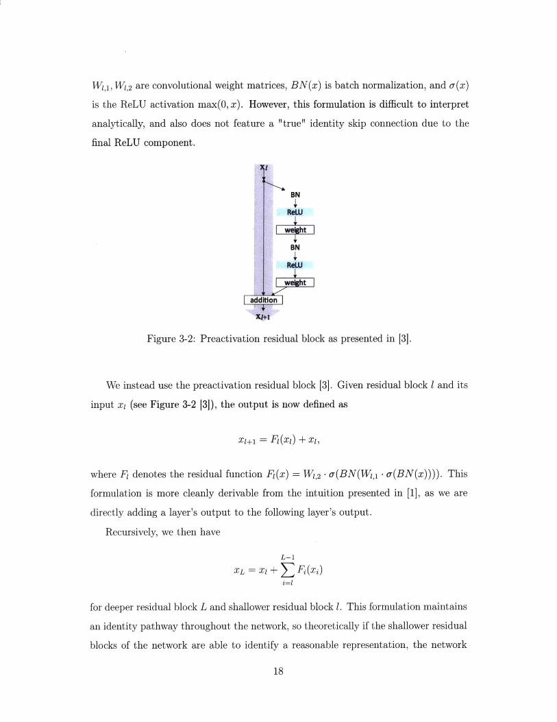
Figure 3-2: Preactivation residual block as presented in [3].
We instead use the preactivation residual block [3]. Given residual block 1 and its
input x, (see Figure 3-2 131), the output is now defined as
X1 = Fi(xi) + xi,
where F denotes the residual function F(x) = W1,2 - o(BN(W,1 -a(BN(x)))). This
formulation is more cleanly derivable from the intuition presented in [1], as we are
directly adding a layer's output to the following layer's output.
Recursively, we then have
L-1
XL = X1 + ( F(xi)i=l
for deeper residual block L and shallower residual block 1. This formulation maintains
an identity pathway throughout the network, so theoretically if the shallower residual
blocks of the network are able to identify a reasonable representation, the network
18

can bypass the remaining layers by using the skip connections (i.e., by sending F(x)
to 0 for later residual blocks).
We can also remove all residual connections to form a standard network, where,
by considering pairs of convolutional layers, we have the analogous equations
x = F(xi)
and
XL = FL-1(FL-2(-- F1(xi))).
19

20

Chapter 4
Empirical Analysis
We perform experiments on CIFAR-10 using residual networks and standard networks
formed by removing the respective residual networks' skip connections. Our objective
is to identify the benefits residual connections provide to network training and explore
how those are brought about. We start by studying the relation between depth and
network performance.
4.1 Representation Learning
One common explanation for residual networks' success is that residual connections
allow for the training of deeper networks that find more complex representations.
However, given a network of a certain depth, it's not clear that adding further layers
to the network is always beneficial - are added layers always guaranteed to learn
new representations? In addition, how does performance compare between a residual
network and a standard network of the same depth?
We can investigate how these networks learn representations by training linear
classifiers on activations of each set of layers (residual blocks in resnets, and pairs
of layers in standard networks) for both networks throughout training. We plot the
converged accuracies of those linear classifiers in Figure 4-2, where blue is used to
identify shallower network layers and red is used to identify deeper network layers.
We find a marked difference in learning behavior. In the standard network, learn-
21
Resnet 34 Unear Classifier Training Accuracy
0 25 5 75 10 125 150 75 2 0
4)O-
25 50 7S 100 125 150EPch
175 20
1234567a910U121314is
2-13-24-35-46-57-68-79-810-911 - 1012-1113- 1214 - 13!15 - 14
*1F
100'
90.
60'
50
70-
3'
2D -
10.
-5.I :
Standard 34 Uirwar Classifier Training Accuracy
0 2S 50 75 100 125 150 175 20
0r
6 2i 50 i5 Ii0 I25 IO 17S 26Ep*Ch
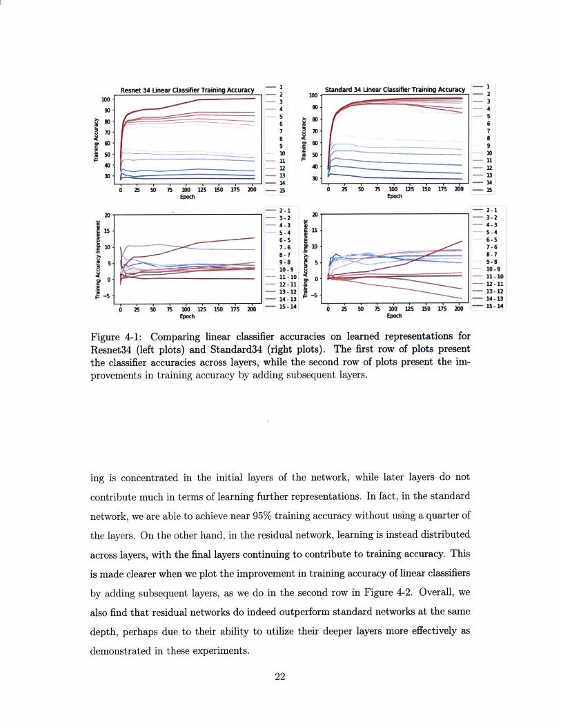
Figure 4-1: Comparing linear classifier accuracies on learned representations forResnet34 (left plots) and Standard34 (right plots). The first row of plots presentthe classifier accuracies across layers, while the second row of plots present the im-provements in training accuracy by adding subsequent layers.
ing is concentrated in the initial layers of the network, while later layers do not
contribute much in terms of learning further representations. In fact, in the standard
network, we are able to achieve near 95% training accuracy without using a quarter of
the layers. On the other hand, in the residual network, learning is instead distributed
across layers, with the final layers continuing to contribute to training accuracy. This
is made clearer when we plot the improvement in training accuracy of linear classifiers
by adding subsequent layers, as we do in the second row in Figure 4-2. Overall, we
also find that residual networks do indeed outperform standard networks at the same
depth, perhaps due to their ability to utilize their deeper layers more effectively as
demonstrated in these experiments.
22
II
I0 -
go
80.
70-
50.
30-
20Is.10-
0
-2345678910
-- 11I- 12
-14
2-13-24-35-46-57-68-79-810-911-10,12-1113-1214-1315- 14
IN - s=:I"-'
10 0'
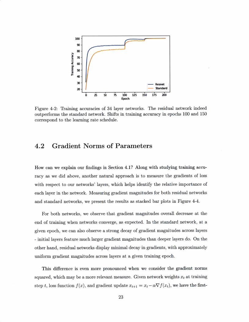
Figure 4-2: Training accuracies of 34 layer networks. The residual network indeed
outperforms the standard network. Shifts in training accuracy in epochs 100 and 150correspond to the learning rate schedule.
4.2 Gradient Norms of Parameters
How can we explain our findings in Section 4.1? Along with studying training accu-
racy as we did above, another natural approach is to measure the gradients of loss
with respect to our networks' layers, which helps identify the relative importance of
each layer in the network. Measuring gradient magnitudes for both residual networks
and standard networks, we present the results as stacked bar plots in Figure 4-4.
For both networks, we observe that gradient magnitudes overall decrease at the
end of training when networks converge, as expected. In the standard network, at a
given epoch, we can also observe a strong decay of gradient magnitudes across layers
- initial layers feature much larger gradient magnitudes than deeper layers do. On the
other hand, residual networks display minimal decay in gradients, with approximately
uniform gradient magnitudes across layers at a given training epoch.
This difference is even more pronounced when we consider the gradient norms
squared, which may be a more relevant measure. Given network weights xt at training
step t, loss function f (x), and gradient update xtel = xt - aVf (xt), we have the first-
23

Resnet 34 Gradient Norms
0 50 100 150 200
2
1!
Standard 34 Gradient
5
0 50 100Epoc
M Initial Conv- Conv 1- Conv 2- Conv 3- Conv 4- Conv 5- Conv 6- Conv 7- Conv 8- Conv 9
Norms Cclv 10- Conv 11
o Cionv 12Conv 13Conv 14Conv 15Ccliv 16
Ccli 17
Conv 19Ccliv 20
w*. Ccnv 21- Cov 22
150 200 -iiii Ccliv 23-Ccliv 24~m Cclv 25-Conv 26m Cciv 27
-Ccliv 28Conv 29
1- Conv 30- Conv 31- Conv 32i Final Unear
Figure 4-3: Gradient norms in 34 layer networks. The results are presented as stackedbar charts across layers, with blue corresponding to shallower layers and red corre-sponding to deeper layers. Gradients in the standard network, unlike the residualnetwork, decay with layer depth.
order Taylor series approximation for loss after applying the update:
f(xt+i) = f(xt) + Vf(xt)T(xt+i - Xt) + o(1lxt+1 - Xt||)
L f(xt) - a I|Vf(xt)1 2 ,
so we see that the change in loss can be approximated by the gradient norm squared.
This complements our previous findings, as we see that gradients decay with layer
depth in standard networks, resulting in much of the learning being dominated by
the initial layers. Residual connections prevent this decay and "redistribute" learning
across layers.
24
25
20
15
5
0

Resnet 34 Gradient Norms"2
VIA.,,~ Yp
SI i i150 200
20
10-
5-
0-
Standard 34 Gradient Norms"
* , h.
6 50 0I& i5oEpoch
Figure 4-4: Gradient norms squared in 34 layer networks.
4.3 Importance of Skip Connections
Now that we have a sense of how training dynamics differ between residual networks
and standard networks, one question that arises is, what are the roles of residual
connections? That is, given a residual block with input x and output F(x) + x as
in Figure 3-2, what are the relative contributions of F(x) and x towards forming
representations? Is this related to the lack of decay in gradients that we observe in
residual networks?
To determine the significance of the residual function F(x), one approach may
be to measure the norms of the convolutional layers' weights; however, this doesn't
take into account the effects of batch normalizations and ReLU activations present in
these residual blocks. We instead proceed by considering the 2 norm ratio IF(x)+xV
25
10 -
5.
0-0 50 100
E poch
I-
I-
2 -
I-
2
200w
I-
I-
I-
I-
Initial ConCon 1Cony 2Cony 3Conv 4Conv 5Conv 6Con 7Com 2Conv 9Con 10Cony 11Conv 12Cony 13Conv 14
Cony 15Cony 16Conv 17Con 15Camy 19Conv 20Conv 21Conv 22Conv 23Conv 24Conv 25Cony 26Cony 27Cony 28Cony 29Cony 30Cony 31Conv 32Final Linear

IIF(x)lI _____ _____, and IIF(x)II for each residual block. The norm ratios F ) I) com-IIF~x)+xI lxi IF(x)+xII' I IF(x) xI ompare the contributions of the input and residual function towards the residual block
output. Then, as a residual block transforms representations using F(x), the ratioJIF(x)II can be thought of as an "empirical norm" of the residual function F that mea-
sures how significantly we change the representation x. For comparison, we can also
compute an analogous ratio IF~x)il in the standard network.
0.8.
&6
0.24- - lxl|Fx+
IF(x)I i JIF(xl + xjl
2 4 Ib 12 14 MBlock
Figure 4-5: Residual block norm ratios. We find that the identity is generally moreimportant than the residual function in forming representations.
Averaging the norm ratios across samples (see Figure 4-5) for each block, we
find that, in residual networks, the ratio |F) | is closer to 1 while IF(x) isiIF(x)+xI iIF(x)+xli
closer to 0 across most residual blocks. This result suggests that residual blocks, in
forming representations, rely heavily on the identity pathway formed through residual
connections, without F(.) needing to change the input representation significantly.
This is supported by the low empirical norms we observe in residual networks
(see Figure 4-6a), with spikes in downsampling residual blocks where we change the
dimensions of our representations. Standard networks, on the other hand, feature
much larger empirical norms.
Combined with our previous results for gradient norms of parameters and repre-
sentation learning, we see that residual connections, by forming an identity pathway,
simplifies the training of individual blocks in residual networks, leading to overall
improved performance.
26

8om
10 12 14 6ck
7.
6
5.
4
3
2
1
2 4 6 1 10 12Block
(b) Standard Network
Figure 4-6: Empirical norm ratios. The residual network, compared to the stan-dard network, features layers with relatively low empirical norms, suggesting that,within a residual block, the residual function does not significantly change the inputrepresentations.
4.4 Optimization Landscape
Our results suggest that residual connections may provide optimization benefits. To
investigate this further, we can study the loss landscapes of our networks by com-
puting the gradient of loss at a particular training epoch and measure how the loss
changes for different step sizes, as in [8].
Epoch 120
10- s0 h 10-'
14
12
30
A I
Epoch 40-MOK
WA" 10-'5b903W
V.S
U.S
M.0
7.35.0
2.5
0010-' 1S.-
Jr.'
a
a4.
0.2
0.
0
StpSkbe
Figure 4-7: Loss landscapes at epochs 0, 40, 80, 120, 160, and 200 for both residualand standard networks. Residual networks are more robust to varied learning ratesand feature smoother loss landscapes than standard networks do.
27
7-
6.
5.
4-
3.
2'
1'-
- IIxF(X)I I IxI
2 4 6
(a) Residual Network
14 16
Epoch 0Rm.
-033.6a.a.a
I'..3
S.
A
Epoch WO
14 -Rs,.
12 2nw
so
4
2
0
Epoch 160-RindW
Epoch 200
-And33
-IIFx)lIxIl 4A"
A .n '
0
2
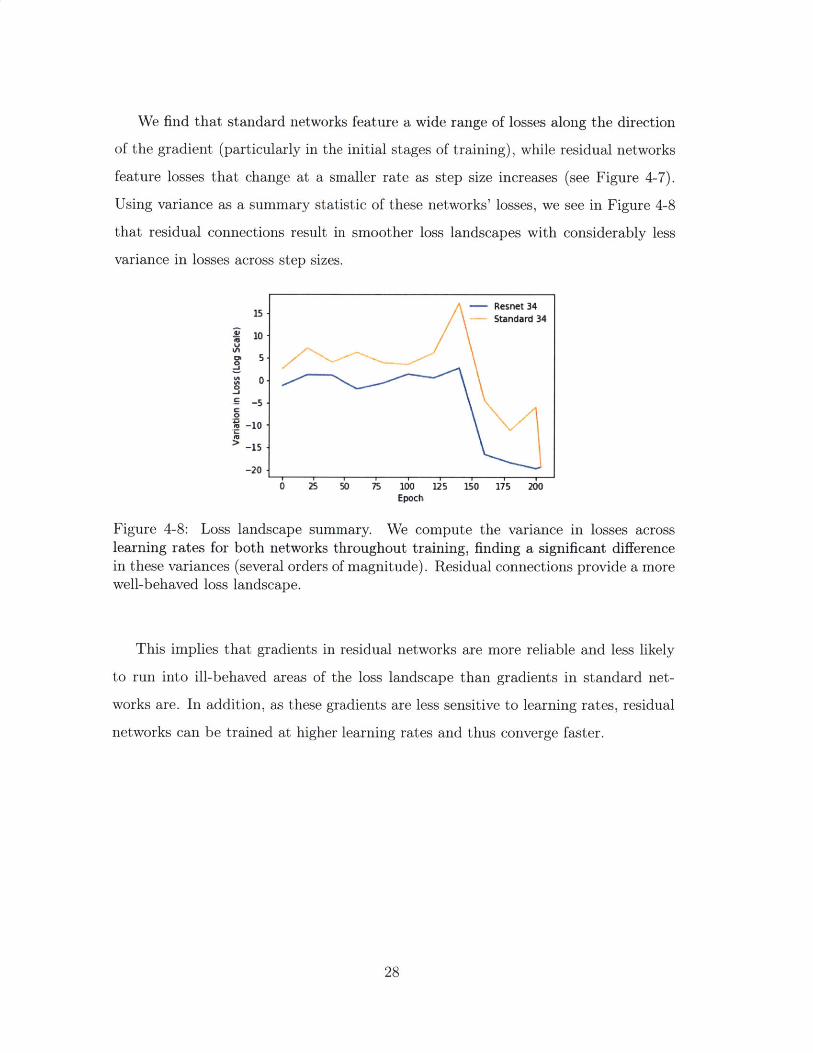
We find that standard networks feature a wide range of losses along the direction
of the gradient (particularly in the initial stages of training), while residual networks
feature losses that change at a smaller rate as step size increases (see Figure 4-7).
Using variance as a summary statistic of these networks' losses, we see in Figure 4-8
that residual connections result in smoother loss landscapes with considerably less
variance in losses across step sizes.
- Resnet 34is- Standard 34
10-
5._ji
0
-10
-15
-20-
0 25 75 100 125 150 175 200Epoch
Figure 4-8: Loss landscape summary. We compute the variance in losses acrosslearning rates for both networks throughout training, finding a significant differencein these variances (several orders of magnitude). Residual connections provide a morewell-behaved loss landscape.
This implies that gradients in residual networks are more reliable and less likely
to run into ill-behaved areas of the loss landscape than gradients in standard net-
works are. In addition, as these gradients are less sensitive to learning rates, residual
networks can be trained at higher learning rates and thus converge faster.
28

Chapter 5
Conclusion
We now have a better understanding of how residual networks outperform standard
networks. We found that residual networks distribute learning across layers so that
each are responsible for learning better representations, while standard networks con-
centrate learning in shallower layers and thus do not make effective use of deeper
layers. Residual connections, by forming an identity pathway, enable this distribu-
tion of learning by making the training of individual blocks easier.
This is supported by our results for gradient norms, where we see non-decaying
gradients with depth in residual networks, as well as our results for empirical norms,
which show that layers in residual networks don't change the representations as much
as layers in standard networks are required to. In addition, we find that residual
connections result in smoother optimization landscapes, which suggests that residual
networks are more robust to varied learning rates.
Some interesting directions to explore include the following:
o We can further investigate optimization benefits of residual connections by run-
ning gradient predictiveness experiments, where we measure the f2 distance
between the loss gradient at a given training step and new gradients observed
while moving along that gradient.
o We can analytically study backpropogation in preactivation resnets and stan-
dard networks to determine whether it might be possible to prevent the decay in
29

gradients in standard networks and improve performance without using residual
connections.
30
k ........... ............. .
Appendix A
Experimental Setup
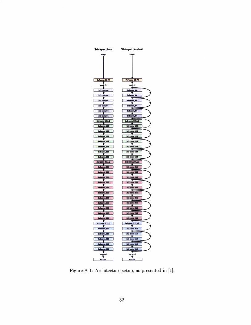
For our experiments, we use the preactivation variants of Resnet 18, Resnet 34, and
Resnet 50 as used in [3]. These residual networks start with an initial convolutional
layer with 16 filters followed by their respective number of residual blocks in three
different stages of dimensions (16, 32, then 64 filters). Each stage of blocks is separated
by a 1 by 1 convolution layer used to change hidden space dimensionality. The
classifier is composed of an average-pool layer, a fully-connected layer, and a final
softmax layer. To create the standard networks, we remove the residual connections,
but leave all remaining components untouched, as in [1]. Figure A-1 [1] illustrates
the Resnet 34 and Standard 34 networks.
For all architectures, we train using SGD for 205 epochs with learning rate 0.1 that
drops to 0.01 at epoch 100 and 0.001 at epoch 150; momentum 0.9; weight decay 0.005;
and data augmentation. In addition, we use batch normalization in both networks, as
we were unable to train standard networks effectively without normalization. Doing
so, we achieve state-of-the-art results for the preactivation resnets (see Table A. 1).
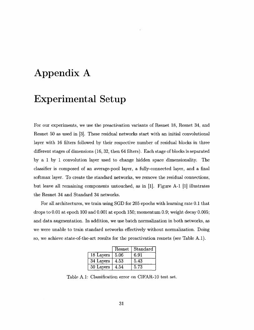
Resnet Standard18 Layers 5.06 6.9134 Layers 4.53 5.4350 Layers 4.54 5.73
Table A.1: Classification error on CIFAR-10 test set.
31
s-I1
--
--
-----.
--- ---
a a
a a
a ~
~ ~ ~ ~
~ a a
91- lo
go- 1 l
f l llo
lo- go lo -
s lo
l 10 be
6-14S3
3 3 3
3
3 3 3 3 2 1 3
3
3 3 3 3 3
Ws
a L-i W9
8 Li L-i LiL iWL i
iLJL j iL j
30
Appendix B
Omitted Figures
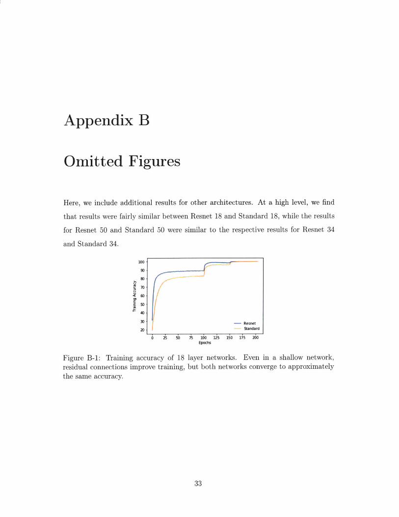
Here, we include additional results for other architectures. At a high level, we find
that results were fairly similar between Resnet 18 and Standard 18, while the results
for Resnet 50 and Standard 50 were similar to the respective results for Resnet 34
and Standard 34.
100
90*
E 70-
60-
s50
40-
20- Resnet
Standard
0 A5 5 0 125 150 175 200Epochs
Figure B-1: Training accuracy of 18 layer networks. Even in a shallow network,residual connections improve training, but both networks converge to approximatelythe same accuracy.
33
womb.-,
100
- - .,nd.-
O0
~40
20
0 2 50 is 100 125 1 50 115 20
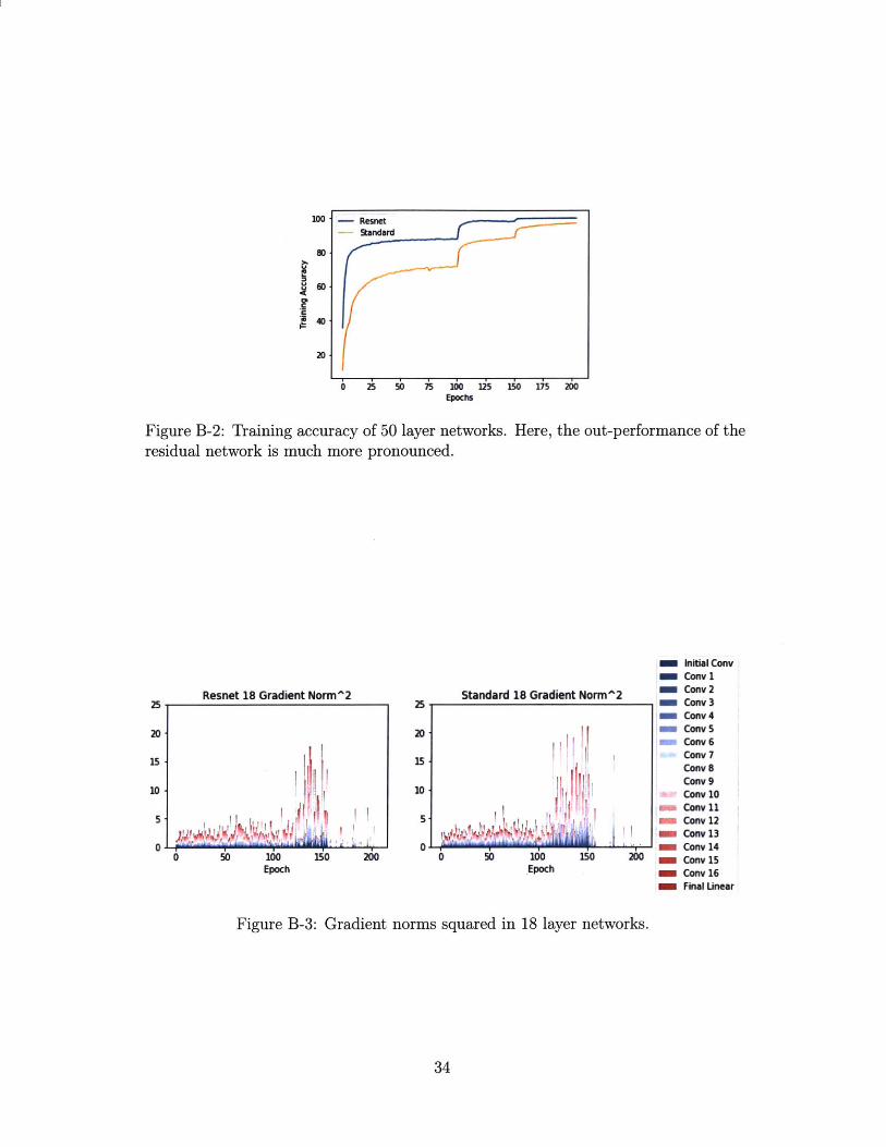
Figure B-2: Training accuracy of 50 layer networks. Here, the out-performance of theresidual network is much more pronounced.
Resnet 18 Gradient Norm^225
20
is
10
5
0
Epoch
Standard 18 Gradient Norm^2
0 50 id0oEpoch
150 200
I nitial Conv- Conv I- Conv 2
Conv 3- Conv 4- Conv 5f Conv6
Conv 7Conv 8Cmiv 9Conv 10
av* Conv 11m Conv 12m Conv 13
m Conv 14-Canvl15
- Conv 16- Final Linear
Figure B-3: Gradient norms squared in 18 layer networks.
34
25
20
15
10
5
0Igo 260

Resnet 50 Gradient Norm^2
0 5b 10Epoch
150 200
70,
60
50 .
40-
30.
20
10.
0-
Standard 50 Gradient
0 50 100Epoch
m Initial Conv- Cony 1- Conv 2
M Conv 3m Conv4
M Conv 5m Conv 6
m Conv 7- Conv eM ConV 9- Conv 10
M Conv 11- Conv 12- Conv 13- Conv 14
Conv 15- Conv 16
m Conv 17
Norm^2 Cony 18- Conv 19
Conv 20Conv 21Cony 22Conv 23Conv 24Conv 25Conv 26Conv 27Conv 28
Conv 32
s Conw 30150 200 w Conv 34- Conv 32- Conv 33- Conv 34- Conv 35
' Conv 36Conv 37
SConv 3- Conv 39- Conv 40- Conv 44
-Cony 42-Cony 43-Conv 4
- Conv 45- Conv 46- Conv 47- Conv 48- Final Linear
Figure B-4: Gradient norms squared in 50 layer networks.
35
60
40-
20.
10.
0.
MW I
A-I-t -"YIW I " ! o kll ,

36
Bibliography
[1] Kaiming He, Xiangyu Zhang, Shaoqing Ren and Jian Sun. Deep Residual Learning
for Image Recognition, 2015; arXiv:1512.03385.
[2] Sergey Ioffe and Christian Szegedy. Batch Normalization: Accelerating Deep
Network Training by Reducing Internal Covariate Shift, 2015; arXiv:1502.03167.
[3] Kaiming He, Xiangyu Zhang, Shaoqing Ren and Jian Sun. Identity Mappings in
Deep Residual Networks, 2016; arXiv:1603.05027.
[4] Andreas Veit, Michael Wilber and Serge Belongie. Residual Networks Behave Like
Ensembles of Relatively Shallow Networks, 2016; arXiv:1605.06431.
[5] David Balduzzi, Marcus Frean, Lennox Leary, JP Lewis, Kurt Wan-Duo Ma and
Brian McWilliams. The Shattered Gradients Problem: If resnets are the answer,
then what is the question?, 2017, PMLR volume 70 (2017); arXiv:1702.08591.
[6] Moritz Hardt and Tengyu Ma. Identity Matters in Deep Learning, 2016;
arXiv:1611.04231.
[7] Ohad Shamir. Are ResNets Provably Better than Linear Predictors?, 2018;
arXiv:1804.06739.
[8] Shibani Santurkar, Dimitris Tsipras, Andrew Ilyas and Aleksander Mqdry. How
Does Batch Normalization Help Optimization?, 2018; arXiv:1805.11604.
37


