Tjalling C. Koopmans Research Institute
Tjalling C. Koopmans Research Institute
Utrecht School of Economics
Utrecht University
Janskerkhof 12
3512 BL Utrecht
The Netherlands
telephone +31 30 253 9800
fax +31 30 253 7373
website www.koopmansinstitute.uu.nl
The Tjalling C. Koopmans Institute is the research institute
and research school of Utrecht School of Economics.
It was founded in 2003, and named after Professor Tjalling C.
Koopmans, Dutch-born Nobel Prize laureate in economics of
1975.
In the discussion papers series the Koopmans Institute
publishes results of ongoing research for early dissemination
of research results, and to enhance discussion with colleagues.
Please send any comments and suggestions on the Koopmans
institute, or this series to [email protected]
ontwerp voorblad: WRIK Utrecht
How to reach the authors
Please direct all correspondence to the first author.
Jacob A. Bikker
De Nederlandse Bank (DNB)
Supervisory Policy Division
Strategy Department
P.O. Box 98
1000 AB Amsterdam
The Netherlands
E-mail: [email protected]
Utrecht University
Utrecht School of Economics
Janskerkhof 12
3512 BL Utrecht
The Netherlands.
This paper can be downloaded at: http:// www.uu.nl/rebo/economie/discussionpapers
Utrecht School of Economics Tjalling C. Koopmans Research Institute
Discussion Paper Series 09-17
An extended gravity model with substitution
applied to international trade
Jacob A. Bikker
Supervisory Policy Division, Strategy Department De Nederlandse Bank
Utrecht School of Economics Utrecht University
July 2009
Abstract
The traditional gravity model has been applied many times to international trade
flows, especially in order to analyze trade creation and trade diversion. However,
there are two fundamental objections to the model: it cannot describe substitutions
between flows and it lacks a cogent theoretical foundation. A newly developed
model, the Extended Gravity Model (EGM), overcomes these objections. The model
shares characteristics of the models of Bergstrand (1985), Andersen and Van
Wincoop (2003), and Redding and Scott (2003). An empirical test on a world-wide
sample of 19 thousand 2005 trade flows strongly rejects the gravity model in favour
of the EGM. The empirical analysis also shows that the gravity model widely
overestimates the influence of the determinants of international trade, which is due
to strong substitution between trade flows, reducing the initial (gravity model)
effects. Substitution determines both trade creation and trade diversion. The EGM
encompasses several models originating in regional economics and can be applied
usefully to a wide set of subjects.
Keywords: bilateral trade, imports, exports, spatial allocation, trade creation, trade
diversion, distance, market access, supplier access, multilateral resistance terms,
remoteness indices.
JEL classification: F1, R12. Acknowledgements The author is grateful to an unkown referee, Gert-Jan Linders and other participants of the Workshop ‘The gravity equation: or why the world is not flat’, Groningen, The Netherlands, October 18-19, 2007, for valuable comments and suggestions and to Jack Bekooij for extensive data support and estimations. This paper enlarges on Bikker (1987), but all empirical results are new.
3
1. Introduction
For over decades the traditional gravity model has been successfully applied to flows of the most widely
varying types, such as migration, flows of buyers to shopping centres, recreational traffic, commuting,
patient flows to hospitals and interregional as well as international trade. The model specifies that a flow
from origin i to destination j is determined by supply conditions at the origin, by demand conditions at the
destination and by stimulating or restraining forces relating to the specific flow between i and j. In a
context of international trade the traditional gravity model usually has the following form:
654321
,,0,βββββββ jijijjiiji PDNYNYX = (1)
where Xi,j is the value of trade between countries i and j, Yk and Nk are the Gross Domestic Product (GDP)
and the size of the population, respectively, of country k, and Di,j and Pi,j denote the distance between
countries i and j and a possible special preference relationship, respectively. The gravity model of bilateral
trade has become the workhorse of applied international economics (Eichengreen and Irwin, 1998) and
has been used in any number of contexts.1 Some authors assume that the size of the population has no
impact, thus β2 = β4 = 0, which renders the resemblance to Newton's Law of Gravity even more obvious.2
The empirical results obtained with the model have always been judged as very good. Deardorff (1998)
argues that the model is sensible, intuitive and hard to avoid as a reduced theoretical model to explain
bilateral trade. Yet the gravity model has some serious imperfections. One is the absence of a cogent
derivation of the model, based on economic theory. Several authors have tried to provide the model with
such a theoretical basis, using models of imperfect competition and product differentiation, notably
Anderson (1979), Bergstrand (1985), Helpman and Krugman (1985) and Anderson and Van Wincoop
(2003), whereas Deardorff (1998) proves that the model is also consistent with the Heckscher-Ohlin trade
theory under perfect competition. However, none of these derivations generates the gravity model exactly
as formulated in Equation (1).3 This equation could only be approximated under a number of restrictive
and unrealistic assumptions, as has been made clear by Bergstrand (1985).
1 Linders (2006) found 200 studies (actually a sample from a much larger set), and provides a selection in his Table
3.1. For an overview, see Anderson and Van Wincoop (2004). 2 E.g. Tinbergen (1962), Pöyhönen (1963a, 1963b), Pulliainen (1963), Geraci and Prewo (1977), Prewo (1978),
Abrams (1980) and Bergstrand (1985). 3 The most restrictive theoretical model of Anderson, Bergstrand, as well as Helpman and Krugman, is a gravity
model with only GDPs as determinants. A less restrictive model has a different functional form (Anderson, Equation
(16) or additional determinants (Bergstrand, Equation (14)).
4
Another imperfection of the gravity model is the absence of substitution between flows.4 Existence of
substitution can be made plausible by economic integration. For example, the accession of Estonia to the
European Union (EU) in 2004 is expected to lead to additional imports by other EU countries of wood,
wood products and paper (their major export product) – that is, gross trade creation, cf. Balassa (1962).
However, EU imports of wood products from other countries may very well decline (somewhat). This
decline – trade diversion – is not described by the gravity model. In the analysis of economic integration,
for which purpose the gravity model is frequently used, trade creation and trade diversion are important
phenomena.
This paper presents an alternative to the gravity model, or rather an extension of it, with substitution
between flows. This extended gravity model shows strong similarities to the models of Bergstrand (1985)
Anderson and Van Wincoop (2003) and Redding and Scott (2003). It can be derived straightforwardly
from supply and demand equations, which provides the model with a theoretical basis. It appears to be a
generalisation of the gravity model which permits empirical testing of the assumptions on which the
gravity model is based. The extended model generates estimation results which – due to a substitution
structure – deviate widely from the gravity model estimates, which underlines the importance of
discerning the substitution structure.
The remainder of this paper consists of the following sections. Section 2 gives the derivation of the model,
called Extended Gravity Model (EGM), from supply and demand equations. Section 3 compares the EGM
with the gravity model, describes its indices of the geo-economic position which establish the model’s
substitution structure and treats econometric issues.5 Section 4 presents estimation results for trade flows
between 178 countries in 2005, tests the EGM against the gravity model and interprets the model
parameters and the indices of the geo-economic position. Section 5 concludes.
2. Derivation of the extended gravity model
The next subsection derives the extended gravity model from a supply and demand system. Alternative
derivations from (among other things) constant-elasticity-of-substitution (CES) preference or utility
4 Glejser and Dramais (1969) have attempted to specify a trade model with substitution but, as they admit, their
model is not without estimation problems. See also Viaene (1982), whose method, however, becomes very complex
when applied to a matrix of trade flows instead of a vector. 5 Many small, mainly technical problems are more or less ignored in this paper, though they were solved. For a more
elaborate introduction of the model, see Bikker and De Vos (1982) or Bikker (1982).
5
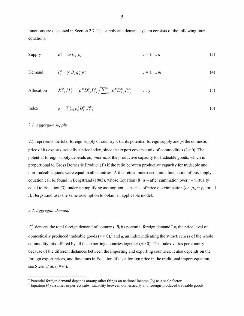
functions are discussed in Section 2.7. The supply and demand system consists of the following four
equations:
Supply λω iisi pCE = i = 1,..., n (3)
Demand πργ jjjdj pqBI = j = 1,..., m (4)
Allocation ∑ ==
n
k jkjkkjijii
d
j
d
ji PDpPDpIX1 ,,,,,
2121 εεµεεµ i ≠ j (5)
Index ∑= =nk jkjkkj PDpq 1 ,,
21 εεµ (6)
2.1. Aggregate supply
siE represents the total foreign supply of country i, Ci, its potential foreign supply and pi the domestic
price of its exports, actually a price index, since the export covers a mix of commodities (λ > 0). The
potential foreign supply depends on, inter alia, the productive capacity for tradeable goods, which is
proportional to Gross Domestic Product (Yi) if the ratio between productive capacity for tradeable and
non-tradeable goods were equal in all countries. A theoretical micro-economic foundation of this supply
equation can be found in Bergstrand (1985), whose Equation (8) is – after summation over j – virtually
equal to Equation (3), under a simplifying assumption – absence of price discrimination (i.e. pi,j = pi for all
i). Bergstrand uses the same assumption to obtain an applicable model.
2.2. Aggregate demand
djI denotes the total foreign demand of country j, Bj its potential foreign demand,
6 pj the price level of
domestically produced tradeable goods (π < 0),7 and qj an index indicating the attractiveness of the whole
commodity mix offered by all the exporting countries together (ρ > 0). This index varies per country
because of the different distances between the importing and exporting countries. It also depends on the
foreign export prices, and functions in Equation (4) as a foreign price in the traditional import equation,
see Stern et al. (1976).
6 Potential foreign demand depends among other things on national income (Yj) as a scale factor.
7 Equation (4) assumes imperfect substitutability between domestically and foreign-produced tradeable goods.
6
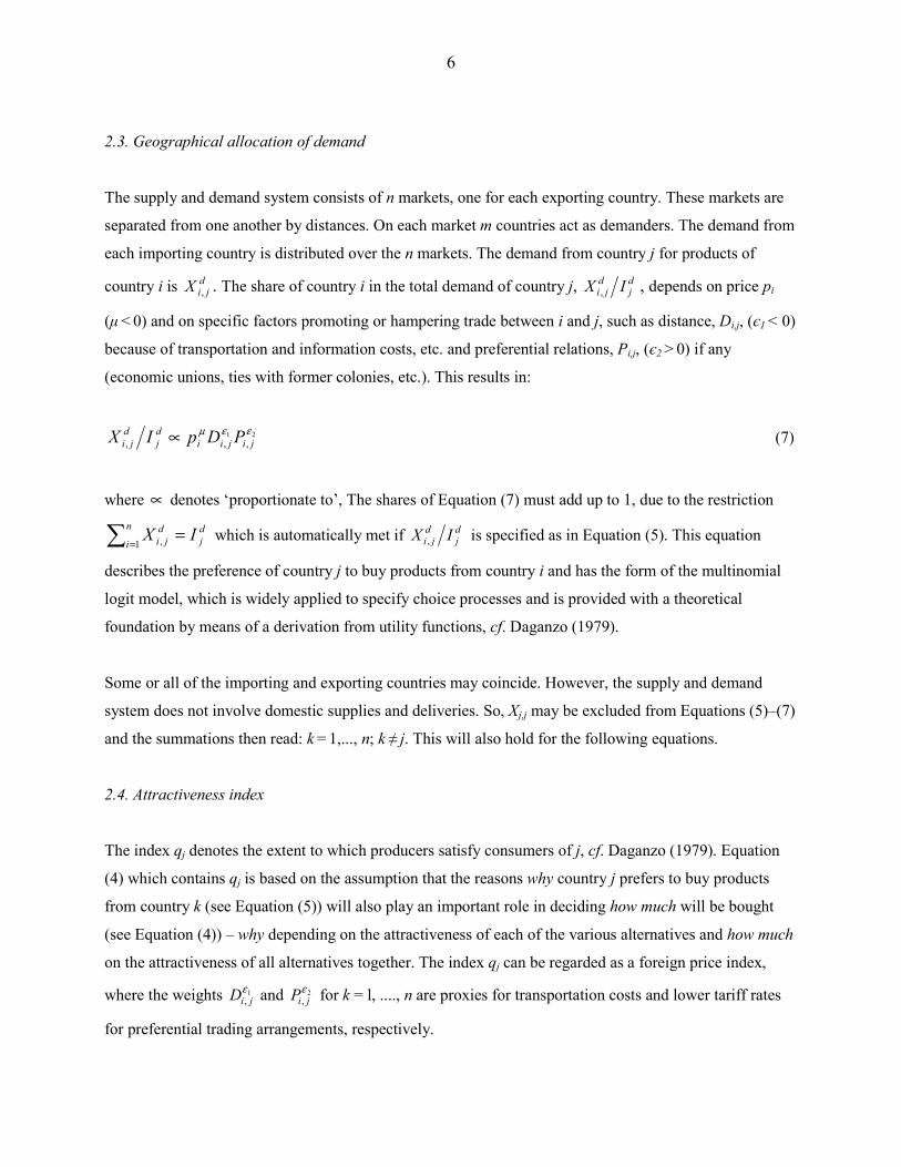
2.3. Geographical allocation of demand
The supply and demand system consists of n markets, one for each exporting country. These markets are
separated from one another by distances. On each market m countries act as demanders. The demand from
each importing country is distributed over the n markets. The demand from country j for products of
country i is djiX , . The share of country i in the total demand of country j,
dj
dji IX , , depends on price pi
(µ < 0) and on specific factors promoting or hampering trade between i and j, such as distance, Di,j, (є1 < 0)
because of transportation and information costs, etc. and preferential relations, Pi,j, (є2 > 0) if any
(economic unions, ties with former colonies, etc.). This results in:
21
,,,
εεµjijii
d
j
d
ji PDpIX ∝ (7)
where ∝ denotes ‘proportionate to’, The shares of Equation (7) must add up to 1, due to the restriction
∑ ==
n
i
d
j
d
ji IX1 , which is automatically met if
dj
dji IX , is specified as in Equation (5). This equation
describes the preference of country j to buy products from country i and has the form of the multinomial
logit model, which is widely applied to specify choice processes and is provided with a theoretical
foundation by means of a derivation from utility functions, cf. Daganzo (1979).
Some or all of the importing and exporting countries may coincide. However, the supply and demand
system does not involve domestic supplies and deliveries. So, Xj,j may be excluded from Equations (5)–(7)
and the summations then read: k = 1,..., n; k ≠ j. This will also hold for the following equations.
2.4. Attractiveness index
The index qj denotes the extent to which producers satisfy consumers of j, cf. Daganzo (1979). Equation
(4) which contains qj is based on the assumption that the reasons why country j prefers to buy products
from country k (see Equation (5)) will also play an important role in deciding how much will be bought
(see Equation (4)) – why depending on the attractiveness of each of the various alternatives and how much
on the attractiveness of all alternatives together. The index qj can be regarded as a foreign price index,
where the weights 1
,εjiD and 2
,εjiP for k = l, ...., n are proxies for transportation costs and lower tariff rates
for preferential trading arrangements, respectively.
7
2.5. Bilateral demand
The bilateral demand equation follows from substitution of (4) and (6) into (5):
21
,,1
,εεµπργ jijiijjj
dji PDppqBX
−= (5')
A theoretical foundation of this equation is given by Bergstrand (1985). Under the assumption of absence
of price discrimination mentioned above, his Equation (4) is in fact equal to Equation (5'), where ϑφjj pq +
is approximated by ξηjj pq .
2.6. Equilibrium
In export market i price pi balances total supply and aggregate demand (for each i):
∑= =ml
dli
si XE 1 , (8)
The equilibrium prices can be derived from:
)/(11 ,,
111][ 21 µλεεπργω −
=−−−
∑= ml lililllii PDBpqCp (9)
Equations (6) and (9) form a simultaneous system: pi depends on ql and pl (note: 1 ≠ i). and ql on pi, et
cetera. It can be proven that this system has a unique solution. This unique solution provides the
equilibrium prices and, by substitution in the other model equations, the equilibrium values of imports,
exports and the index. The equilibrium model obtained in this way cannot be applied empirically in its
present form, because the simultaneous set of equilibrium prices pi from Equation (9) and index values qj
from Equation (6) can only be calculated from exogenous variables, given the unknown parameters π, λ
and µ. An empirically useful model can be obtained if the unidentified system of prices and indices is
rewritten into an identified set of indices αi and βj. These indices are defined as follows:
8
∑= =−m
l lilillli PDBpq1 ,,1 21 εεπρα )/( γωµλ
ii Cp−= (10)
∑ ==
n
k jkjkkj PDp1 ,,
21 εεµβ )( jq=
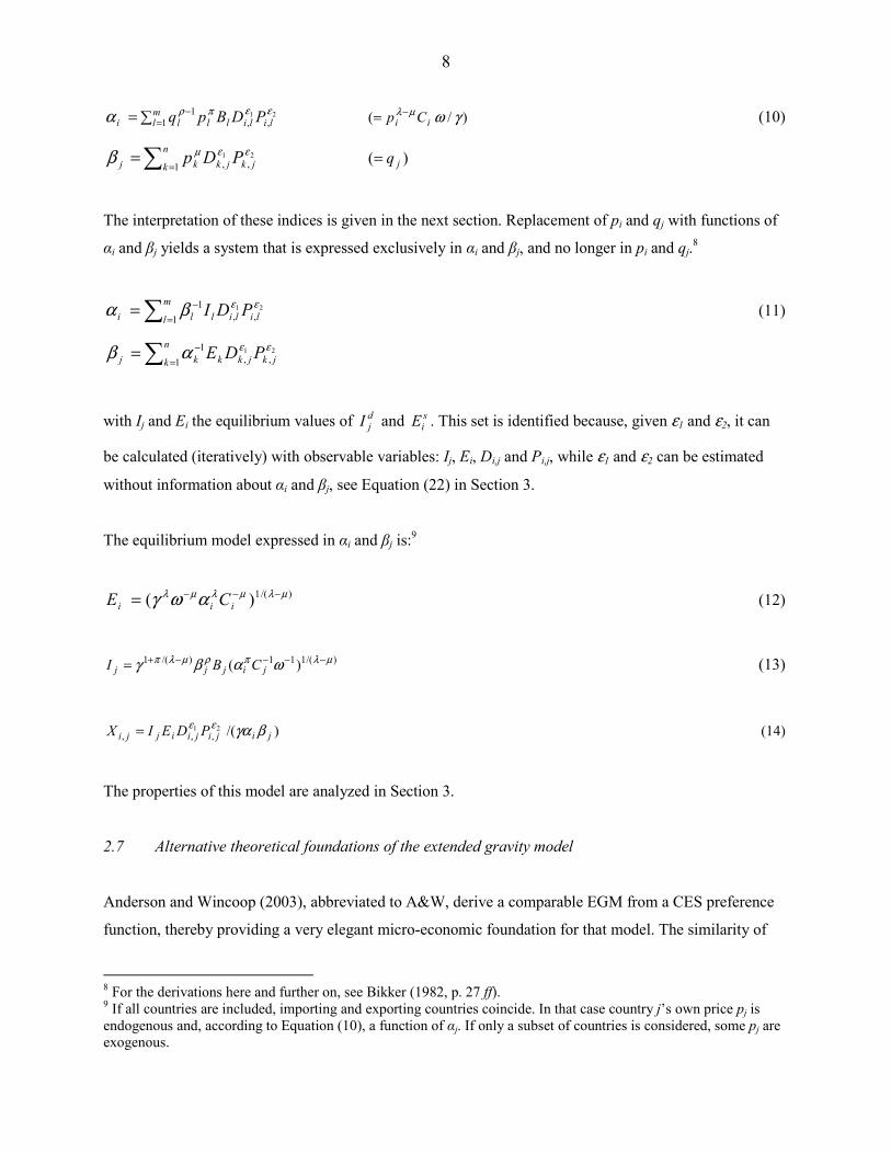
The interpretation of these indices is given in the next section. Replacement of pi and qj with functions of
αi and βj yields a system that is expressed exclusively in αi and βj, and no longer in pi and qj.8
∑ =
−=m
l lililli PDI1 ,,
1 21 εεβα (11)
∑ =
−=n
k jkjkkkj PDE1 ,,
1 21 εεαβ
with Ij and Ei the equilibrium values of djI and s
iE . This set is identified because, given ε1 and ε2, it can
be calculated (iteratively) with observable variables: Ij, Ei, Di,j and Pi,j, while ε1 and ε2 can be estimated
without information about αi and βj, see Equation (22) in Section 3.
The equilibrium model expressed in αi and βj is:9
)/(1)( µλµλµλ αωγ −−−= iii CE (12)
)/(111)/(1)(
µλπρµλπ ωαβγ −−−−+= jijjj CBI (13)
)/(21
,,, jijijiijji PDEIX βγαεε= (14)
The properties of this model are analyzed in Section 3.
2.7 Alternative theoretical foundations of the extended gravity model
Anderson and Wincoop (2003), abbreviated to A&W, derive a comparable EGM from a CES preference
function, thereby providing a very elegant micro-economic foundation for that model. The similarity of
8 For the derivations here and further on, see Bikker (1982, p. 27 ff).
9 If all countries are included, importing and exporting countries coincide. In that case country j’s own price pj is
endogenous and, according to Equation (10), a function of αj. If only a subset of countries is considered, some pj are
exogenous.
9
their results to ours becomes clear when the above Equations (11) of the indices αi and βj are compared to
Equations (10) and (11) of the A&W price indices Пi and Pj. Note that A&W end up with two (scaled)
price indices for each country, reflecting prices of, respectively, imports and exports. Only under a further
symmetric trade barrier assumption (discussed below) and a ‘balanced trade’ assumption do the two price
indices coincide, that is, Пi = Pi (Anderson, 2009). The symmetric trade barrier assumption, however, is
far from trivial, as shown below.
Bergstrand (1985) derives a type of EGM using double constant-elasticity-of-substitution (CES) utility
functions for consumers and double constant-elasticity-of-transformation (CET) joint production surfaces
for producers. He specifies supply and demand for each trade flow Xij, but links their aggregates over i and
j to the respective countries’ national incomes. Bergstrand’s equilibrium model for Xij resembles Equation
(14) and the model of A&W, but deviates in that it uses different substitution elasticities on the foreign
and domestic markets.
Redding and Scott (2003) and Redding and Venables (2004) derive an EGM rather comparable to that of
A&W and this paper, using Cobb-Douglas preference and production functions. They define (foreign)
market access and and (foreign) supplier access identical to our indices αi and βj, which can be rewritten in
prices and price indices. Their model is more restricted as the exponential parameters of market access,
supplier access and distance are all equal to σ–1 or 1–σ. The ‘new economic geography’ wage level in
their model is a function of these access variables, which in turn depend on prices. This approach has also
been applied by Bosker and Garretsen (2009) and Boulhol (2009). ). Behrens et al. (2007) develop a
gravity model, which is a simplification of the various models above, as it contains only one set of indices,
supplier access, instead of two (ignoring market access).10 Similarly, Anderson (1979) presents in
Equation (16) a gravity model with market access, ignoring supplier access.
For the application of the gravity model to world trade, the A&W foundation is most elegant. However,
the derivation in Sections 2.1-2.6 above has two advantages. First, it applies to a wider set of applications.
Earlier, the EGM has been applied to flows of hospital patients from resident areas to hospitals (Bikker
and De Vos, 1992a). Other potential applications are the international trade in single commodities (such as
oil), commuter traffic, migration flows, and flows of shoppers to shopping centres, students to schools,
tourists to holiday destinations, et cetera. In those cases, origin and destination regions do not coincide,
10 This would be equivalent to imposing µ = 0 in Equation (5) and (6), see Bikker (1982, p. 38).
10
contrary to the symmetry between origin and destination regions commonly found in general international
trade.11
Second, Sections 2.1-2.6 explain clearly that the attractiveness of a country’s trade partners (or ‘other
countries’), given its geographical location, may differ substantially for its imports and its exports. These
sections propose the distinct indices αi and βj as measures of the geographical attractiveness of,
respectively, exports and imports. A&W come up with two distinct sets of price indices, defined similarly
to these indices, but the two sets of price indices coincide under the symmetry trade barrier assumption.
Such symmetry is likely with respect to distances and preferential relations due to economic unions, ties
with former colonies, et cetera. International trade between two countries depends also heavily on the
correlation between the supply by product types of the exporting country and the demand by product types
of the importing country. This applies in particular to commodities. Behrens et.al. (2007) and Bergstrand
et al. (2009) stress that trade costs are far from symmetric. Symmetry may also be absent for other omitted
variables. This is also evident from the empirical application of the EGM: in 2005, the trade barrier
residuals (that is, omitted variables) of the trade flows Xi,j and Xj,i (that is: uij and uji) have a markedly low
correlation at 0.2, pointing to quite limited symmetry. Particularly in the absence of a variable for the
correlation between demanded and supplied goods, this argues for the use of both sets of indices, that is,
repudiation of the symmetry trade barrier assumption.
Finally, we notice a few further, though not essential, differences between A&Ws foundation and the
derivation given above. A&W include demand for and supply to domestic consumption.12 This inclusion
is essential for their derivation, because their (theoretical) model is based on countries’ total demand and
total supply. Two remarks are in order. First, inclusion of domestic consumption and production is elegant
as substitution may be expected between domestic and foreign demand. For domestic consumption and
production it is quite common to distinguish between tradeables and non-tradeables (e.g. Anderson, 1979;
Bergstrand, 1985). A&W assume demand substitution among exporter countries to be the same as
substitution between foreign and domestic demand, which is less plausible as the substitution between
foreign tradeables and domestic non-tradeables is likely to be close(r) to zero. For that reason, Bergstrand
assumes different degrees of substitution between demand from various foreign countries and between
foreign and domestic demand. In practice, statistics do not exactly distinguish between domestic
tradeables and non-tradeables. For that reason, Section 2.2 excludes domestic tradeables (as empirical
11 The symmetric trade barrier assumption does not hold true for the international trade of a commodity with a
limited number of supply countries. Furthermore, trade data sets may be incomplete, for instance because some trade
flows are reported as zero or are in fact absent. 12 Note that consumption also includes investment goods.
11
application goes with practical issues), but includes the price level of domestically produced tradeable
goods (pj) in the demand equation (4) so as to take possible substitution into account. This results in a
more complex equilibrium equation of imports (13), deviating from the A&W equation.13
There is a second argument why inclusion of domestic consumption and production, the diagonal elements
of the trade matrix, are often excluded in practice, although they may appear elegant in the theoretical
derivations. In the gravity model all trade flows depend on the distances between pairs of exporting and
importing countries, but, in practice, the specification of the distance between producers and consumers
within a country is a thorny issue (e.g. Anderson and Smith, 1999, p. 29, Head and Mayer, 2009). Often
no trade costs are assumed, that is, the effect of distance is set at zero (ln(Dii) = 0). For a better solution,
though somewhat arbitrary, see Equation (15) in Bosker and Garretsen (2009). Behrens et al. (2007, p. 8)
raise the problem that explanatory variable GDPi is not exogenous to the dependent variable ‘domestic
consumption’ (or production) Xi,i. Note that the diagonal elements of matrix X may be either included in
or deleted from the derivations in Sections 2.1-2.6 above without any change in the theoretical results,
apart from the respective interpretation: in the inclusion implies that total production and consumption are
described (in fact, national income),14 whereas exclusion means that the model refers to imports and
exports only.15 Hence, it is not needed here to make a principle choice.
3. THE EXTENDED GRAVITY MODEL
For empirical application of the equilibrium model thus obtained, it is necessary to specify the concepts of
potential foreign supply, Ci, and demand, Bj. Potential foreign supply depends on productive capacity,
proxied by Gross National Product, Yi, and on market size (approximated by population, Ni). The latter is
based on the assumption of economies of scale: the larger N is, the higher is the number of production
lines for which the country will meet the minimum market size for efficient market production. The larger
N, therefore, the larger the domestic market will be in relation to the foreign market, and the smaller the
potential foreign supply. Other lines of reasoning for Ni in the export equations can be found in Leamer
and Stern (1970), Krugman (1979, 1980) and Brada and Mendez (1983), see also Linnemann (1966),
Leamer (1974) and Chenery and Syrquin (1975). An alternative explanatory variable is the country’s
surface area Ai, which may reflect size, occurrence of mineral resources, and average distance to foreign
13 In the empirical application the import equation is used in its simplified form, see Equation (17) below.
14 Note that if the EGM described all production and consumption (hence include diagonal elements), π, i.e. the
elasticity of the (competing) price level of domestically produced tradeable goods, would equal 0 in Equation (4). 15 A third option would be to include only (domestic) tradeable goods in the diagonal elements.
12
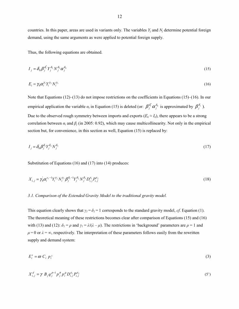
countries. In this paper, areas are used in variants only. The variables Yj and Nj determine potential foreign
demand, using the same arguments as were applied to potential foreign supply.
Thus, the following equations are obtained.
432*1
0δδδδ αβδ jjjjj NYI = (15)
321
0γγγαγ iiii NYE = (16)
Note that Equations (12)–(13) do not impose restrictions on the coefficients in Equations (15)–(16). In our
empirical application the variable αi in Equation (15) is deleted (or: 4
*1 δδ αβ jj is approximated by 1δβ j ).
Due to the observed rough symmetry between imports and exports (Ek ≈ Ik), there appears to be a strong
correlation between αi and βj (in 2005: 0.92), which may cause multicollinearity. Not only in the empirical
section but, for convenience, in this section as well, Equation (15) is replaced by:
321
0δδδβδ jjjj NYI = (17)
Substitution of Equations (16) and (17) into (14) produces:
21321321
,,11'
0,εεδδδγγ βαγ jijijjjii
yiji PDNYNYX
−−= (18)
3.1. Comparison of the Extended Gravity Model to the traditional gravity model.
This equation clearly shows that γ1 = δ1 = 1 corresponds to the standard gravity model, cf. Equation (1).
The theoretical meaning of these restrictions becomes clear after comparison of Equations (15) and (16)
with (13) and (12): δ1 = ρ and γ1 = λ/(λ – µ). The restrictions in ‘background’ parameters are ρ = 1 and
µ = 0 or λ = ∞, respectively. The interpretation of these parameters follows easily from the rewritten
supply and demand system:
λω iisi pCE = (3)
21
,,1
,εεµπργ jijiijjj
dji PDppqBX
−= (5’)
13
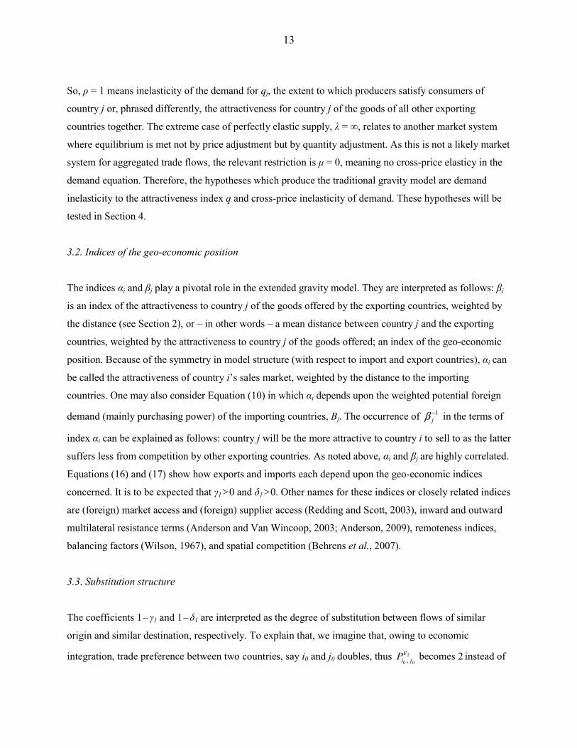
So, ρ = 1 means inelasticity of the demand for qj, the extent to which producers satisfy consumers of
country j or, phrased differently, the attractiveness for country j of the goods of all other exporting
countries together. The extreme case of perfectly elastic supply, λ = ∞, relates to another market system
where equilibrium is met not by price adjustment but by quantity adjustment. As this is not a likely market
system for aggregated trade flows, the relevant restriction is µ = 0, meaning no cross-price elasticy in the
demand equation. Therefore, the hypotheses which produce the traditional gravity model are demand
inelasticity to the attractiveness index q and cross-price inelasticity of demand. These hypotheses will be
tested in Section 4.
3.2. Indices of the geo-economic position
The indices αi and βj play a pivotal role in the extended gravity model. They are interpreted as follows: βj
is an index of the attractiveness to country j of the goods offered by the exporting countries, weighted by
the distance (see Section 2), or – in other words – a mean distance between country j and the exporting
countries, weighted by the attractiveness to country j of the goods offered; an index of the geo-economic
position. Because of the symmetry in model structure (with respect to import and export countries), αi can
be called the attractiveness of country i’s sales market, weighted by the distance to the importing
countries. One may also consider Equation (10) in which αi depends upon the weighted potential foreign
demand (mainly purchasing power) of the importing countries, Bj. The occurrence of 1−
jβ in the terms of
index αi can be explained as follows: country j will be the more attractive to country i to sell to as the latter
suffers less from competition by other exporting countries. As noted above, αi and βj are highly correlated.
Equations (16) and (17) show how exports and imports each depend upon the geo-economic indices
concerned. It is to be expected that γ1 > 0 and δ1 > 0. Other names for these indices or closely related indices
are (foreign) market access and (foreign) supplier access (Redding and Scott, 2003), inward and outward
multilateral resistance terms (Anderson and Van Wincoop, 2003; Anderson, 2009), remoteness indices,
balancing factors (Wilson, 1967), and spatial competition (Behrens et al., 2007).
3.3. Substitution structure
The coefficients 1 – γ1 and 1 – δ1 are interpreted as the degree of substitution between flows of similar
origin and similar destination, respectively. To explain that, we imagine that, owing to economic
integration, trade preference between two countries, say i0 and j0 doubles, thus 2
00 ,
εjiP becomes 2 instead of
14
1, see Equation (18). The terms of 0i
α and 0j
β , which correspond to the trade flow between i0 and j0 also
contain the factor 2
00 ,
εjiP . If γ1 = δ1 = 0, total exports of country i0 and total imports of country j0 – cf.
Equations (16) and (17) – do not change: additional trade between i0 and j0 is entirely at the expense of
other trade flows of similar origin or similar destination – thus trade diversion without (net) trade creation,
or full substitution.16 By contrast, if γ1 = δ1 = 1 – the traditional gravity model case – Equation (18) shows
17
that there will be no substitution at all – trade creation without trade diversion. Doubling of 00 , ji
X say from
x to 2x, will, if γ1 = δ1 = 1, lead to more exports from country i0 to a value of x and more imports by
country j0 to the same amount. Thus we conclude that 1 – γ1 and 1 – δ1 reflect the degree of substitution
between export flows and import flows, respectively. If γ1 and δ1 exceed 1, complementarity between
flows will outweigh substitution.
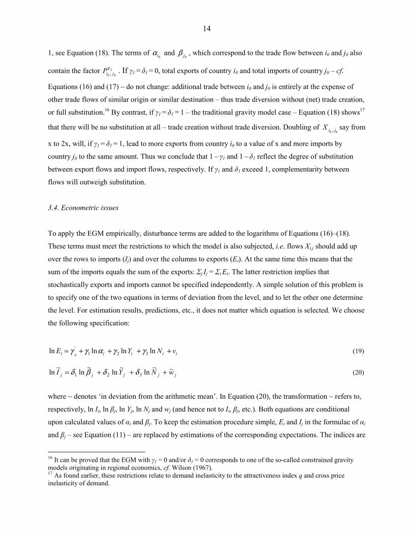
3.4. Econometric issues
To apply the EGM empirically, disturbance terms are added to the logarithms of Equations (16)–(18).
These terms must meet the restrictions to which the model is also subjected, i.e. flows Xi,j should add up
over the rows to imports (Ij) and over the columns to exports (Ei). At the same time this means that the
sum of the imports equals the sum of the exports: Σj Ij = Σi Ei. The latter restriction implies that
stochastically exports and imports cannot be specified independently. A simple solution of this problem is
to specify one of the two equations in terms of deviation from the level, and to let the other one determine
the level. For estimation results, predictions, etc., it does not matter which equation is selected. We choose
the following specification:
iiiii vNYE ++++= lnlnlnln 321'
0γγαγγ (19)
jjjjj wNYI ~~ln
~ln
~ln
~ln 321 +++= δδβδ (20)
where ~ denotes ‘in deviation from the arithmetic mean’. In Equation (20), the transformation ~ refers to,
respectively, ln Ii, ln βj, ln Yj, ln Nj and wj (and hence not to Ii, βj, etc.). Both equations are conditional
upon calculated values of αi and βj. To keep the estimation procedure simple, Ei and Ij in the formulae of αi
and βj – see Equation (11) – are replaced by estimations of the corresponding expectations. The indices are
16 It can be proved that the EGM with γ1 = 0 and/or δ1 = 0 corresponds to one of the so-called constrained gravity
models originating in regional economics, cf. Wilson (1967). 17 As found earlier, these restrictions relate to demand inelasticity to the attractiveness index q and cross price
inelasticity of demand.
15
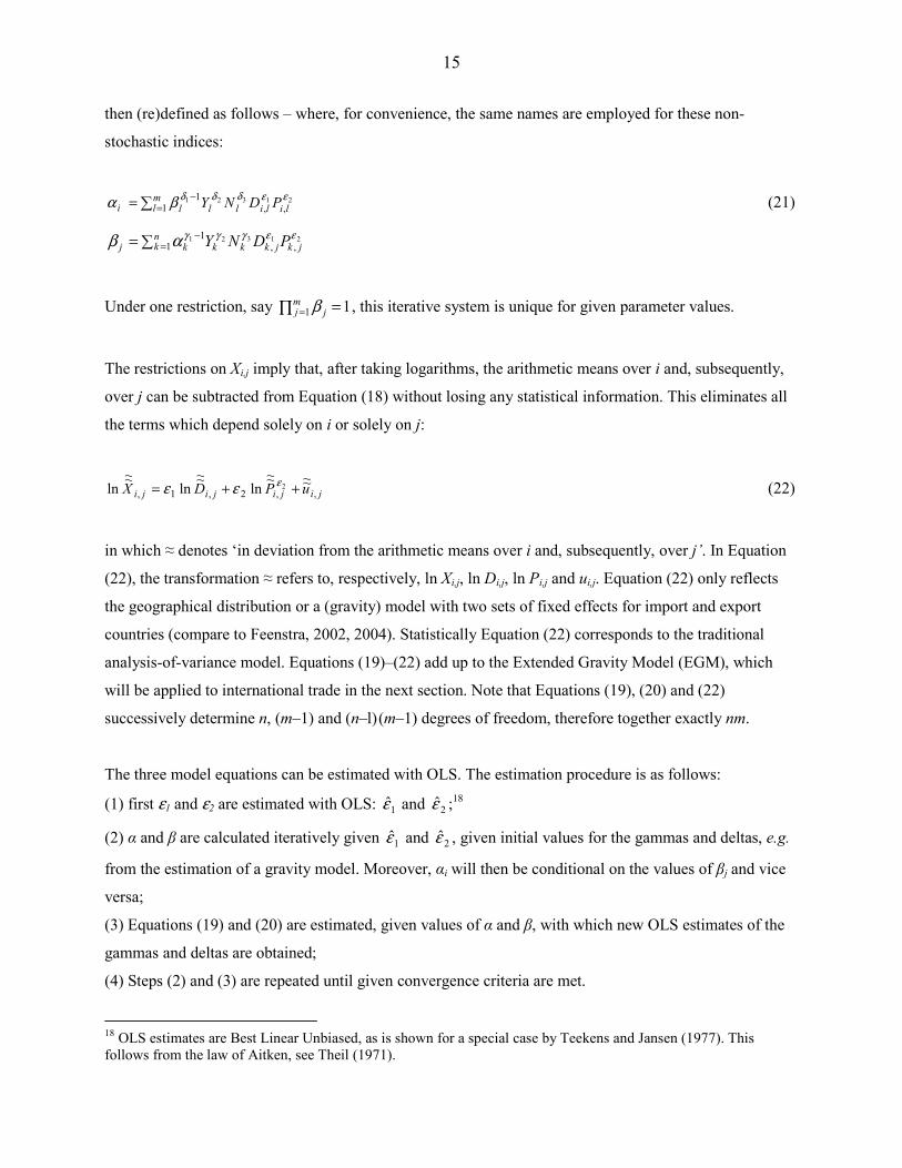
then (re)defined as follows – where, for convenience, the same names are employed for these non-
stochastic indices:
∑ =−
= ml lilillli PDNY1 ,,
1 21321 εεδδδβα (21)
∑= =−n
k jkjkkkkj PDNY1 ,,1 21321 εεγγγαβ
Under one restriction, say 11 =∏ =mj jβ , this iterative system is unique for given parameter values.
The restrictions on Xi,j imply that, after taking logarithms, the arithmetic means over i and, subsequently,
over j can be subtracted from Equation (18) without losing any statistical information. This eliminates all
the terms which depend solely on i or solely on j:
jijijiji uPDX ,,2,1,
~~~~
ln~~
ln~~
ln 2 ++=εεε (22)
in which ≈ denotes ‘in deviation from the arithmetic means over i and, subsequently, over j’. In Equation
(22), the transformation ≈ refers to, respectively, ln Xi,j, ln Di,j, ln Pi,j and ui,j. Equation (22) only reflects
the geographical distribution or a (gravity) model with two sets of fixed effects for import and export
countries (compare to Feenstra, 2002, 2004). Statistically Equation (22) corresponds to the traditional
analysis-of-variance model. Equations (19)–(22) add up to the Extended Gravity Model (EGM), which
will be applied to international trade in the next section. Note that Equations (19), (20) and (22)
successively determine n, (m–1) and (n–l) (m–1) degrees of freedom, therefore together exactly nm.
The three model equations can be estimated with OLS. The estimation procedure is as follows:
(1) first ε1 and ε2 are estimated with OLS: 1ε̂ and 2ε̂ ;18
(2) α and β are calculated iteratively given 1ε̂ and 2ε̂ , given initial values for the gammas and deltas, e.g.
from the estimation of a gravity model. Moreover, αi will then be conditional on the values of βj and vice
versa;
(3) Equations (19) and (20) are estimated, given values of α and β, with which new OLS estimates of the
gammas and deltas are obtained;
(4) Steps (2) and (3) are repeated until given convergence criteria are met.
18 OLS estimates are Best Linear Unbiased, as is shown for a special case by Teekens and Jansen (1977). This
follows from the law of Aitken, see Theil (1971).
16
If the disturbance terms are normally distributed, the total likelihood function can be formulated and
therefore the most likely estimates can be calculated. These estimates may depart slightly from the OLS
estimates, since through the indices in Equation (21) the imports and exports equations may contain
information about the estimates of ε1 and ε2 from the allocation Equation (22). Maximum likelihood
estimates can be calculated with a numerical estimation procedure.
4. Estimation results
This section applies both the traditional gravity model and the EGM to international aggregated trade
flows between 178 countries. As diagonal elements relate to domestic supplies and deliveries, they have
not been included here, so there are in principle 178 x 177 individual trade flows. Part of the flows
(12,156) have been recorded as zero due to rounding or to actual absence of trade, leaving 19,350 non-
zero flows.19 The figures date back to 2005. Information about the data used is given in Appendix A.
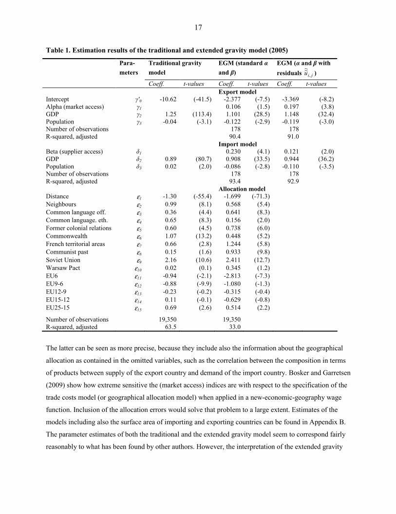
Table 1 shows estimation results of the common gravity model and our extended version of it. A number
of preference variables have been added to the model, which will be explained below. We present results
of two variants of the EGM, the EGM with standard α and β, as introduced above, and the EGM based on
α and β which include the allocation residuals jiu ,
~~ :
)~~exp()
~~( ,1 ,,
1 21321
liml lilillli uPDNYu ∑= =
− εεδδδβα (23)
∑= =−n
k jkjkjkkkkj uPDNYu 1 ,,,
1)
~~exp()~~( 21321 εεγγγαβ
19 Bikker and De Vos (1992b) aim at solving estimation bias due to zero trade flows.
17
Table 1. Estimation results of the traditional and extended gravity model (2005)
Para-
meters
Traditional gravity
model
EGM (standard α
and β)
EGM (α and β with
residuals jiu ,
~~ )
Coeff. t-values Coeff. t-values Coeff. t-values
Export model
Intercept γ'0 -10.62 (-41.5) -2.377 (-7.5) -3.369 (-8.2)
Alpha (market access) γ1 0.106 (1.5) 0.197 (3.8)
GDP γ2 1.25 (113.4) 1.101 (28.5) 1.148 (32.4)
Population γ3 -0.04 (-3.1) -0.122 (-2.9) -0.119 (-3.0)
Number of observations 178 178
R-squared, adjusted 90.4 91.0
Import model
Beta (supplier access) δ1 0.230 (4.1) 0.121 (2.0)
GDP δ2 0.89 (80.7) 0.908 (33.5) 0.944 (36.2)
Population δ3 0.02 (2.0) -0.086 (-2.8) -0.110 (-3.5)
Number of observations 178 178
R-squared, adjusted 93.4 92.9
Allocation model
Distance ε1 -1.30 (-55.4) -1.699 (-71.3)
Neighbours ε2 0.99 (8.1) 0.568 (5.4)
Common language off. ε3 0.36 (4.4) 0.641 (8.3)
Common language. eth. ε4 0.65 (8.3) 0.156 (2.0)
Former colonial relations ε5 0.60 (4.5) 0.738 (6.0)
Commonwealth ε6 1.07 (13.2) 0.448 (5.2)
French territorial areas ε7 0.66 (2.8) 1.244 (5.8)
Communist past ε8 0.15 (1.6) 0.933 (9.8)
Soviet Union ε9 2.16 (10.6) 2.411 (12.7)
Warsaw Pact ε10 0.02 (0.1) 0.345 (1.2)
EU6 ε11 -0.94 (-2.1) -2.813 (-7.3)
EU9-6 ε12 -0.88 (-9.9) -1.080 (-1.3)
EU12-9 ε13 -0.23 (-0.2) -0.315 (-0.4)
EU15-12 ε14 0.11 (-0.1) -0.629 (-0.8)
EU25-15 ε15 0.69 (2.6) 0.514 (2.2)
Number of observations 19,350 19,350
R-squared, adjusted 63.5 33.0
The latter can be seen as more precise, because they include also the information about the geographical
allocation as contained in the omitted variables, such as the correlation between the composition in terms
of products between supply of the export country and demand of the import country. Bosker and Garretsen
(2009) show how extreme sensitive the (market access) indices are with respect to the specification of the
trade costs model (or geographical allocation model) when applied in a new-economic-geography wage
function. Inclusion of the allocation errors would solve that problem to a large extent. Estimates of the
models including also the surface area of importing and exporting countries can be found in Appendix B.
The parameter estimates of both the traditional and the extended gravity model seem to correspond fairly
reasonably to what has been found by other authors. However, the interpretation of the extended gravity
18
model will appear to be quite different. Before examining the parameter estimates in detail, we will
discuss the major difference between the gravity model and the EGM.
4.1. Comparison of the gravity model with the EGM
The gravity model is a special case of the EGM. The models are equal if two sets of restrictions are
imposed on the latter. The first set concerns the substitution between flows, which is lacking in the gravity
model, owing to the two restrictions γ1 = δ1 = 1. The second set regards the error structure. Comparison of
Equations (19), (20) and (22) with (14) shows that the EGM has an error with a variance components
structure: ijji vwu ++ ~~~, . This error structure reduces to an ordinary one (ui,j) only if a special relation
between the standard deviations σv, σw and σu holds:20
m σv = n σw = σu (24)
A Wald test on the two restrictions γ1 = δ1 = 1 (that is, a gravity model with a variance components error
structure) makes clear that these restrictions (and thus the traditional gravity model) are rejected in favour
of the EGM with a well-nigh maximum conviction. Earlier calculations have revealed that the – from an
economic point of view – less crucial restrictions on the standard deviations of the errors terms are
rejected with even more confidence, supporting the rejection of the traditional gravity model (Bikker,
1987).
The EGM has also been compared with the gravity model in a second way. This way is inspired by the
fact that interest in total imports and exports per country is often greater than in individual trade flows.
When the country aggregates of the gravity model are compared to those of the EGM, the gravity model
again proves to be strongly defeated by the EGM – for their standard deviations of total exports and total
imports residuals appear to be well over 50% higher than those of the EGM. Moreover, the gravity model
rather heavily overestimates the actual totals, but this could be due in part to problems of interpreting the
constant in a log-linear model, see Teekens and Koerts (1972).
20 Some elements of the analysis become a little more complex if observations are lacking, as is the case here. One
element is the restriction (24) which in this empirical application is actually formulated somewhat differently.
Another is the reduction of Equation (18) to (22): the transformation ≈ now requires more calculations. A third
relates to the Jacobian required to transform the dependent variables of the EGM into those of the gravity model. In
all cases the problems are purely technical and have been fully solved, see Bikker (1982).
19
4.2. Interpretation of the EGM parameter estimates
On the face of it, most parameter values of the gravity model and of the EGM do not differ much,
especially not in the equations for imports and exports, whereas it is exactly here that some differences
might be expected, because of the diverging coefficients of the indices (0.106 versus 1 and 0.230 versus 1,
see Table 1, standard α and β). Closer examination, however, shows that the EGM parameters clearly have
a different meaning from those of the gravity model. This is because each explanatory variable also occurs
in both indices and therefore affects the modelled trade flow along three channels. Therefore, the overall
effect is not immediately apparent. Of course, the effect of a variable can always be determined with a
model simulation. However, it is also possible to interpret the parameter estimates analytically. For it can
be demonstrated that the effect of (changes in) Y or N from the export equation on Xi,j equals γ2 or γ3,
respectively, each multiplied by:
δ1 / (γ1 + δ1 – γ1 δ1) (25)
that is, provided there is an equal proportional change in Y or N in all exporting countries. We call the
coefficients multiplied by (25) overall-effect elasticities. They are immediately comparable with the
parameters β1 and β2 from the gravity model. The overall effect elasticities of the import equation (apart
from δ1 itself) and the distribution model are obtained analogously by multiplying the corresponding
parameters with, respectively:
γ1 / (γ1 + δ1 – γ1 δ1) and γ1 δ1 / (γ1 + δ1 – γ1 δ1) (25)
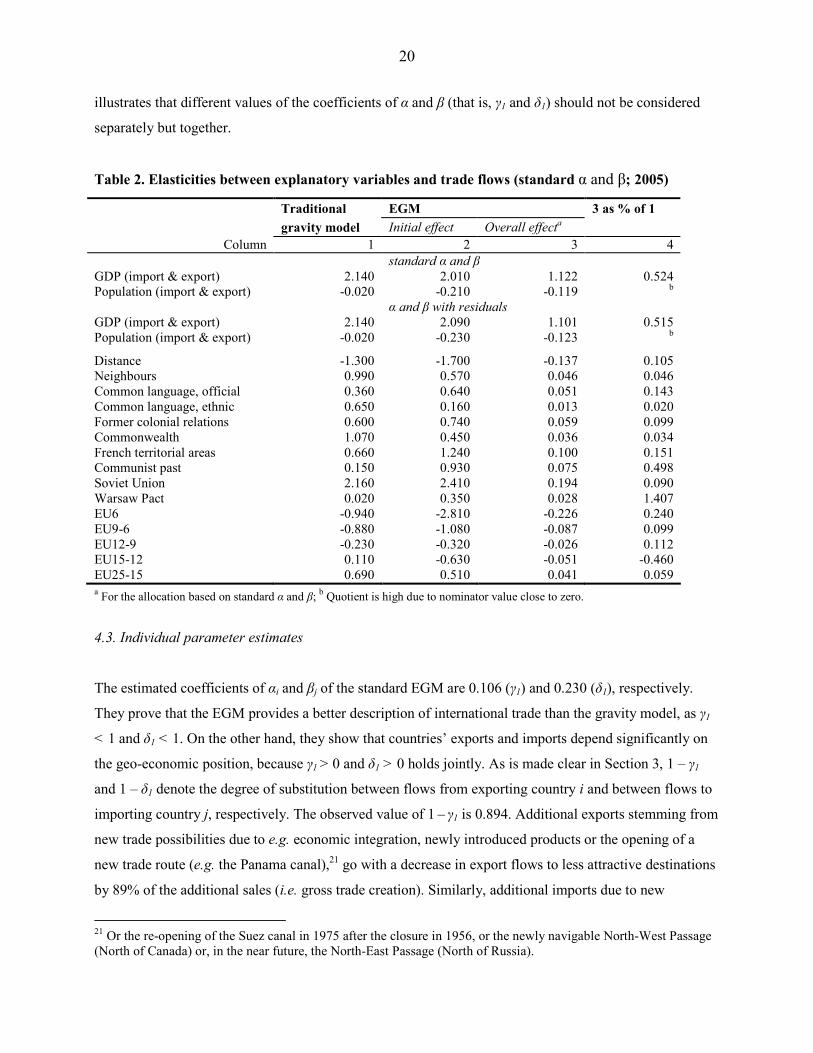
The overall effect elasticities are shown in Column 3 of Table 2. The effects on trade flows of GDP and
population of the imports and exports model have been added together because in this empirical example
importing and exporting countries coincide, so that a change in e.g. all GDPs will affect the modelled
trade flow along the import side as well as the export side. Remarkably, nearly all overall effects of the
EGM are much smaller than those of the gravity model. Owing to substitution, part of the initial effects
leak away. This effect is similar to the lower ‘border effect’ between the US and Canada measured by the
EGM of Anderson and Van Wincoop (2003), including the multilateral resistance terms, compared to the
traditional gravity model of McCallum (1995), see also Behrens et al. (2007, p. 8).
If we recalculate the elasticities in Table 2 on the EGM with α and β with residuals jiu ,
~~ instead of the
standard EGM α and β, we obtain largely identical results (see third and fourth row in Table 2). This
20
illustrates that different values of the coefficients of α and β (that is, γ1 and δ1) should not be considered
separately but together.
Table 2. Elasticities between explanatory variables and trade flows (standard α and β; 2005)
Traditional EGM 3 as % of 1
gravity model Initial effect Overall effecta
Column 1 2 3 4
standard α and β
GDP (import & export) 2.140 2.010 1.122 0.524
Population (import & export) -0.020 -0.210 -0.119 b
α and β with residuals
GDP (import & export) 2.140 2.090 1.101 0.515
Population (import & export) -0.020 -0.230 -0.123 b
Distance -1.300 -1.700 -0.137 0.105
Neighbours 0.990 0.570 0.046 0.046
Common language, official 0.360 0.640 0.051 0.143
Common language, ethnic 0.650 0.160 0.013 0.020
Former colonial relations 0.600 0.740 0.059 0.099
Commonwealth 1.070 0.450 0.036 0.034
French territorial areas 0.660 1.240 0.100 0.151
Communist past 0.150 0.930 0.075 0.498
Soviet Union 2.160 2.410 0.194 0.090
Warsaw Pact 0.020 0.350 0.028 1.407
EU6 -0.940 -2.810 -0.226 0.240
EU9-6 -0.880 -1.080 -0.087 0.099
EU12-9 -0.230 -0.320 -0.026 0.112
EU15-12 0.110 -0.630 -0.051 -0.460
EU25-15 0.690 0.510 0.041 0.059
a For the allocation based on standard α and β;
b Quotient is high due to nominator value close to zero.
4.3. Individual parameter estimates
The estimated coefficients of αi and βj of the standard EGM are 0.106 (γ1) and 0.230 (δ1), respectively.
They prove that the EGM provides a better description of international trade than the gravity model, as γ1
< 1 and δ1 < 1. On the other hand, they show that countries’ exports and imports depend significantly on
the geo-economic position, because γ1 > 0 and δ1 > 0 holds jointly. As is made clear in Section 3, 1 – γ1
and 1 – δ1 denote the degree of substitution between flows from exporting country i and between flows to
importing country j, respectively. The observed value of 1 – γ1 is 0.894. Additional exports stemming from
new trade possibilities due to e.g. economic integration, newly introduced products or the opening of a
new trade route (e.g. the Panama canal),21 go with a decrease in export flows to less attractive destinations
by 89% of the additional sales (i.e. gross trade creation). Similarly, additional imports due to new
21 Or the re-opening of the Suez canal in 1975 after the closure in 1956, or the newly navigable North-West Passage
(North of Canada) or, in the near future, the North-East Passage (North of Russia).
21
attractive import possibilities go with a 77% decrease in competitive import flows. Apparently, ignoring
substitution would generate disastrous model forecasts.
The EGM coefficients of the GDPs of import and export countries suggest that a 1% growth of the world
economy leads to a somewhat more than proportional increase in international trade flows of 1.22%, see
Column 3 of Table 2. This corresponds to past observations. This contrasts, however, with the more than
‘quadratic’ increase in trade suggested by the gravity model, see Column 1. Remarkably, exports outgrow
GDP (γ2 is 1.10), whereas import grow lags behind GDP grow (δ2 = 0.91). The size of the population
reflects scale economies: large countries are more autarkic. Their effects are in line with expectations, but
the population coefficients are small compared to the values observed in the past. Apparently, the optimal
scale becomes larger over time: even large countries cannot afford to produce for the domestic market
alone.
Distance is the major allocation variable. Its coefficient in the EGM approaches the parameter in
Newton’s law. The coefficient is higher than observed in the past, as also found in a survey by Linders
(2006). Our value is at the highest end of the observed estimates. This may reflect a world-wide
convergence of prices, so that transportation costs count more heavily (Estevadeordal et al. (2003) and
Anderson and Van Wincoop, 2004). Further, the allocation model includes the following preferential
dummy variables, which reflect the intangible barriers to trade related to cultural differences, institutional
conditions and differences other than those embodied by mere distance (Obstfeld and Rogoff, 2000;
Deardorff 2004): whether or not two countries are contiguous, share a common official language, have a
common language due to ethnic composition of the population, have ever had a colonial link, are both
members of the Commonwealth or the Francophone ‘Communauté Financière Africaine’ (CFA), are both
former communist countries, are both former members of the Soviet Union or the former Warsaw Pact, or,
finally, are both EU Member States, with a further distinction by membership of the 6, 9, 12, 15, or 25
Member Community. For instance, EU9-6 refers to (additional) trade of Denmark, Ireland and the UK
with the first six EU Member States as well as their mutual trade. Most preferential coefficients are in line
with expectations, that is, have positive signs; many are more or less consistently significant. Many ex-
colonial preferences are weaker than observed in the past. Apparently, ex-colonial ties have worn thinner
in the course of time. A remarkable exception in the expected effects is EU membership, where the older
cohorts have negative rather than positive signs.22 This might be due to measurement errors: even a minor
22 Intra-EU trade is larger than the trade between the other countries in Western Europe, as shown by Aitken (1973).
Abrams (1980) and Bergstrand (1985), who used European trade flow figures only. Negative EU coefficients point
to a level of EU trade which is nevertheless lower than the level of world trade, after correction for the size of the
countries (Y and N), for distances, etc.
22
error in the determination of the – relatively small – distances between EU countries would greatly affect
the EU coefficients, as the EU countries lie closely together (see Head and Mayer, 2009). Comparisons
over time could reveal the true EU impact on international trade.23 The R-squares make clear that we are
able to explain only a minor part of the variation in the allocation (R2 = 33.0), compared to that in the
imports (R2 = 92.9) and exports (R
2 = 91.0).
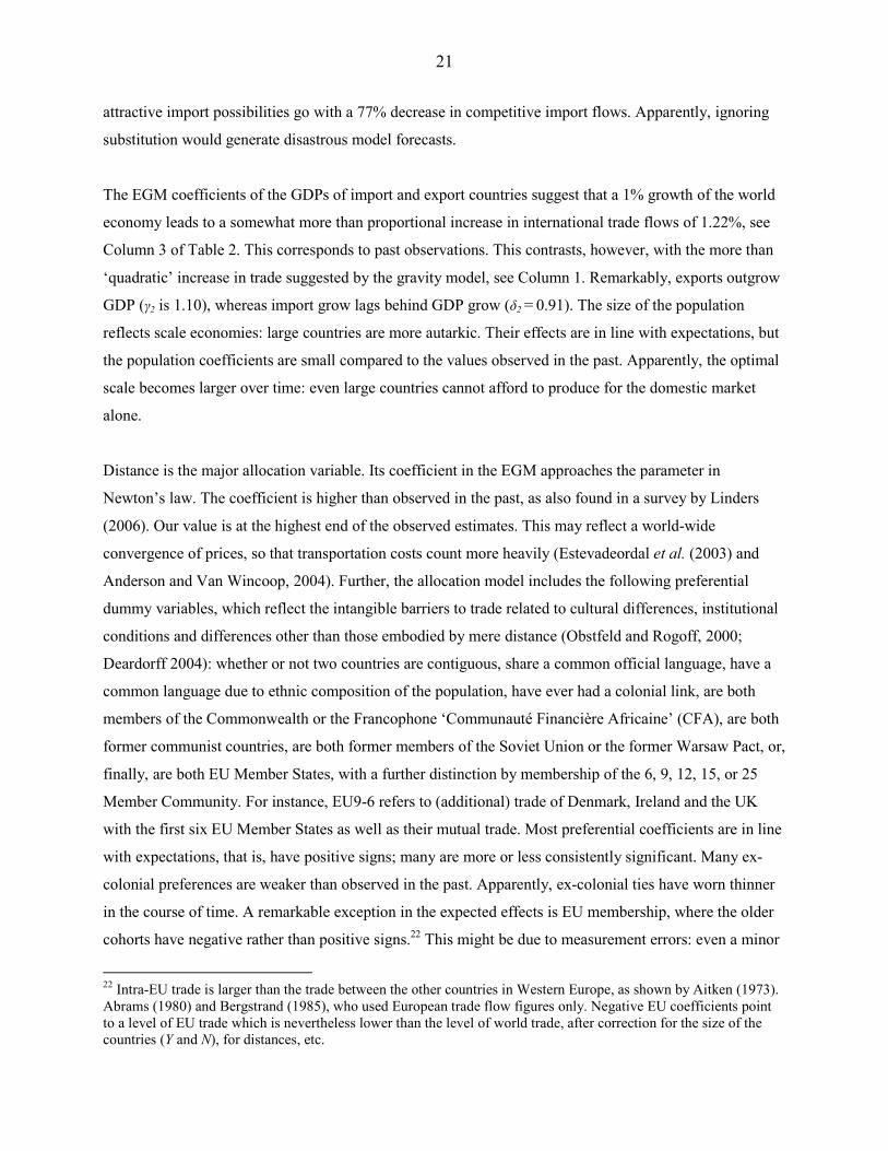
4.4. The indices of the geo-economic position
The index αi can be called the attractiveness of country i’s sales market, weighted by the distances to the
respective importing countries, whereas βj is an index of the attractiveness to country j of the goods
offered by the respective exporting countries, again weighted by distance. Table 3 presents regional means
for both indices, with and without allocation residuals, all expressed in deviation from their geometric
world-wide mean. We first discuss the indices without residuals, reflecting best the geographical position
of countries. The location of the European countries clearly is a favourable one – with, in economic terms,
many countries with a large economy situated closely together. This holds even more for Central and
Eastern Europe and the former Soviet Union (former Soviet Union members have strong mutual
preferences), which lie near Western Europe. North American countries benefit from the USA with its
gigantic economy, while the USA itself lies less favourably. South America, Africa and, particularly,
Oceania, have more isolated locations, whereas the Middle East and the Rest of Asia take intermediate
positions.
The allocation residual jiu ,
~~ reflects mainly the correlation between the composition in terms of products
between the supply of country i and the demand of country j. If they are included in the indices, the
alpha’s of countries with sought-after products rise. Oil producing countries in the Middle East and
countries producing raw material in Africa become more attractive, whereas regions with less mineral
resources, such as Europe and Asia lose attraction. The position of importing countries is affected less
strongly.
23 Comparison of earlier estimates for 1974 and 1959 – before the EU could make any considerable contribution
towards economic integration – shows that the relative preference for other EU countries over 1959-1974 rose by
76% (Bikker, 1987). In other words, it is not the level of the EU dummy, but the change therein that provides
quantitative information about economic integration. However, such a shift has not been observed over 1975-2005.
23
Table 3. Geo-economic trade positions of exports (α) and imports (β) per region
Without residuals jiu ,
~~ With residuals jiu ,
~~
Alpha’s Beta’s Alpha’s Beta’s
Western Europe 1.86 1.73 0.40 1.36
Central and Eastern Europe a 3.23 2.27 1.67 2.89
Former Soviet Union 4.46 2.70 1.20 1.96
North and Central America 0.98 1.59 0.81 1.14
South America 0.51 0.63 0.43 1.00
Middle East 1.13 0.80 2.82 0.91
Rest of Asia 0.93 1.17 0.56 0.60
Oceania 0.32 0.47 1.22 0.50
North-Western Africa 0.60 0.57 1.77 0.74
South-Eastern Africa 0.38 0.37 1.05 0.56 a Excluding the former Soviet Union Member countries.
Explanation: The indices are from the EGM without area and are expressed in deviation from their world-wide geometric mean.
5. CONCLUSIONS
The Extended Gravity Model (EGM) proves to be a useful extension of the traditional gravity model. A
test of 2005 figures on international trade flows quite convincingly rejects the gravity model in favour of
the more generalised EGM. Apparently, EGMs substitution structure, which does not preclude a relatively
simple estimation procedure, is a much more realistic model for international trade. In general, the degree
of substitution between trade flows appears to be around 80% or more. This structure, in principle, allows
for an analysis of economic integration in terms of trade diversion and trade creation. The EGM leads to
conclusions regarding the effect of the determinants of trade flows, which deviate clearly from those
reached by means of the gravity model: the traditional gravity model strongly overestimates the effects of
changes in determinants. In addition, the EGM provides index values of the geo-economic trade position
for all countries concerned, both of the attractiveness of a country’s sales market, weighted by the
distances to the respective importing countries, and of the attractiveness to each country of the goods
offered by the respective exporting countries, again weighted by distance.
The EGM can be applied usefully to a wide variety of subjects, see e.g. Bikker and De Vos (1992a) on
patient flows to hospitals. Apart from the log-linear regression model, the EGM also encompasses the
production-constrained, the attraction-constrained and the so called doubly-constrained gravity models
originating in regional economics, cf. Wilson (1967), and of the analysis-of-variance model, see Cesario
(1973) and Wansbeek (1977). From a statistical point of view, the EGM has well-defined properties.
Empirical application requires more calculations than in the case of the traditional gravity model.
However, the applications show clearly that the effort pays off.
24
References
Abrams, R.K.: International Trade Flows under Flexible Exchange Rates, Economic Review, Federal
Reserve Bank of Kansas City, 1980, 3-10.
Aitken, N.D.: The Effect of the EEC and EFTA on European Trade: A Temporal Cross-Section Analysis.
American Economic Review 63 (1973), 881-892.
Anderson, J.E.: A Theoretical Foundation for the Gravity Equation, American Economic Review 69
(1979), 106-116.
Anderson, M.A., and S.L.S. Smith, Canadian provinces in would trade: engagement and detachment,
Canadian Journal of Economics 32 (1999), 22-38.
Anderson, J.E. and Van Wincoop, E., Gravity with gravitas: a solution to the border puzzle, American
Economic Review 93 (2003), 170-192.
Anderson J.E. and Van Wincoop, E., Trade costs, Journal of Economic Literature 42 (2004), 691-751.
Anderson, J.E., The Incidence of Gravity in General Equilibrium, In: Brakman, S., and P.A.G. van
Bergeijk (eds), The Gravity Model in International Trade: Advances and Applications, Cambridge
University Press, 2009, Chapter 2, (forthcoming).
Balassa, B.: The Theory of Economic Integration, London: Allen and Unwin, 1962.
Behrens, K., C. Ertur and W. Koch, Dual gravity: using spatial econometrics to control for multilateral
resistance, CORE Discussion Paper 2007/59, 2007.
Bergstrand, J.H.: The Gravity Equation in International Trade: Some Microeconomic Foundations and
Empirical Evidence. Review of Economics and Statistics 67 (1985), 471-481.
Bergstrand, J.H., P. Egger and M. Larch, Approximating General Equilibrium Impacts of Trade
Liberalization using the Gravity Equation, In: Brakman, S., and P.A.G. van Bergeijk (eds), The
Gravity Model in International Trade: Advances and Applications, Cambridge University Press,
2009, Chapter 3, (forthcoming).
Bikker, J.A.: Vraag-aanbodmodellen voor stelsels van geografisch gespreide markten. toegepast op de
internationale handel en op ziekenhuisopnamen in Noord-Nederland (In Dutch; Supply-demand
Models for Systems of Geographically Dispersed Markets. with Applications to International Trade
Flows and Hospital Admissions in the North of the Netherlands). Amsterdam: Free University
Publishing Company, 1982.
Bikker, J.A., An international trade flow model with substitution: an extension of the gravity model,
Kyklos 40 (1987), 315-337.
Bikker, J.A. and De Vos, A.F.: Interdependent Multiplicative Models for Allocation and Aggregates: A
Generalization of Gravity Models, Research Paper 80, Actuarial Science and Econometrics
Department, Amsterdam: Free University, 1982.

25
Bikker, J.A., and De Vos, A.F., A regional supply and demand model for inpatient hospital care,
Environment and Planning A 24 (1992a), 1097-1116.
Bikker, J.A., and De Vos, A.F., An international trade flow model with zero observations: an extension of
the Tobit model, Cahiers Economiques de Bruxelles 135 (1992b), 379-404.
Bosker, E.M., and H. Garretsen, Trade costs, market access and economic geography: Why the empirical
specification of trade costs matters, In: Brakman, S., and P.A.G. van Bergeijk (eds), The Gravity
Model in International Trade: Advances and Applications, Cambridge University Press, 2009,
Chapter 6, (forthcoming).
Boulhol, H., The Contribution of Economic Geography to GDP Per Capita, In: Brakman, S., and P.A.G.
van Bergeijk (eds), The Gravity Model in International Trade: Advances and Applications,
Cambridge University Press, 2009, Chapter 11 (forthcoming).
Cesario, F.J.: A Generalized Trip Distribution Model. Journal of Regional Science 13 (1973), 223-247.
Chenery, H. and Syrquin, M.: Patterns of Development, 1950-1970, World Bank, Oxford University
Press, 1975.
Daganzo, C.: Multinomial Probit, the Theory and its Application to Demand Forecasting, New York:
Academic Press, 1979.
Deardorff, A.V., Determinants of bilateral trade: does gravity work in a neoclassical world?, in : J. Frenkel
(ed.), The Regionalization of the World Economy, 7-28, Chicago, University of Chicago Press,
1998.
Deardorff, A.V., Local comparative advantage: trade costs and the pattern of trade, Research Seminar in
International Economics Discussion Paper, University of Michican nr. 500, Ann Arbor, 2004.
Eichengreen, B., and Irwin, D.A., The role of history in bilateral trade flows, in: J.A. Frankel (ed.), The
Regionalization of the World Economy, 33-57, Chicago, University of Chicago Press, 1998.
Estevadeordal, A., Frantz, B., and Taylor, A.M., The rise and fall of world trade, 1870-1939, Quarterly
Journal of Economics 68 (2003), 359-408.
Feenstra, R.E., Border effects and the gravity equation: consistent methods for estimation, Scottish
Journal of Political Economy 49 (2002), 491-506.
Feenstra, R.E., Advanced International Trade: Theory and Evidence, Princeton and Oxford, NJ: Princeton
University Press, 2004.
Geraci, V.J. and Prewo, W.: Bilateral Trade Flows and Transport Costs. Review of Economics and
Statistics 59 (1977), 67-74.
Glejser, H. and Dramais, A.: A Gravity Model of Interdependent Equations to Estimate Flow Creation and
Diversion. Journal of Regional Science 9 (1969), 439-449.
26
Head, K., and Mayer, T. L‘effet frontière: une mesure de l‘intégration économique, Economie et Prévision
152-153 (2002), 71-92.
Head, K., and Mayer, T., Illusory border effects: distance mismeasurement inflates estimates of home bias
in trade, In: Brakman, S., and P.A.G. van Bergeijk (eds), The Gravity Model in International Trade:
Advances and Applications, Cambridge University Press, 2009, Chapter 5, (forthcoming).
Helpman, E. and Krugman, P.R.: Market Structure and Foreign Trade: Increasing Returns, Imperfect
Competition, and the International Economy, Cambridge (USA), 1985.
Krugman, P.R.: Increasing Returns. Monopolistic Competition and International Trade, Journal of
International Economics 9 (1979), 469-479.
Krugman, P.R.: Scale Economies, Product Differentiation and the Pattern of Trade, American Economic
Review 70 (1980), 950-959.
Leamer, E.E. and Stern, R.M.: Quantitative International Economics. Boston: Allyn and Bacon, 1970.
Leamer, E.E.: Nominal Tariff Averages with Estimated Weights. Southern Economic Journal 41 (1974),
34-45.
Linders, G.J.M., Intangible barriers to trade; the impact of institutions, culture and distance on pattern of
trade, Tinbergen Institute Research Series nr. 371, Tinbergen Institute, 2006.
Linnemann, H.: An Econometric Analysis of International Trade Flows. Amsterdam: North-Holland
Publishing Company, 1966.
McCallum, J., National borders matter: Canada-US regional trade patterns, American Economic Review
85 (1995), 615-623.
Obstfeld, M., and Rogoff, K., The six major puzzles in international macro-economics: is there a common
cause?, In: NBER Macro-economics Annual 15, 339-390, Cambridge, MA: the MIT Press, 2000.
Pelzman, J.: Trade Creation and Trade Diversion in the Council of Mutual Economic Assistance. 1954-70.
American Economic Review 67 (1977), 713-722.
Pölyhönen, P.: A tentative model for the volume of trade between countries, Welwirtschaftliches Archiv
90 (1963a), 93-100.
Pölyhönen, P.: Toward a General Theory of International Trade. Economiska Samfundets Tidskrift 16
(1963b), 69-77.
Prewo, W.: Determinants of the Trade Pattern among OECD Countries from 1958 to 1974, Jahrbücher für
Nationalökonomie und Statistik 193 (1978), 341-358.
Pulliainen, K.: A World Trade Study: An Econometric Model of the Pattern of the Commodity Flows of
International Trade in 1948-60. Economiska Samfundets Tijdskrift 16 (1963), 78-91
Redding, S. and P.K. Scott, Distance, Skill Deepening and Development: Will Peripheral countries Ever
Get Rich?, Journal of Development Economics 72 (2003), 515-541.
27
Redding, S. and A.J. Venables, Economic Geography and International Inequality, Journal of
International Economics 62 (2004), 53-82.
Stern, R.M.: Francis J. and Schumacher. B.: Price Elasticities in International Trade, London and
Basingstoke, 1976.
Teekens, R. and Koerts, J.: Some Statistical Implications of the Log Transformation of Multiplicative
Models, Econometrica 40 (1972), 793-813.
Teekens, R. and Jansen, R.: A Note on the Estimation of a Multiplicative Allocation Model. Research
Report 7703, Econometric Institute, Rotterdam: Erasmus University, 1977.
Theil, H.: Principles of Econometrics. New York: John Wiley and Sons, 1971.
Tinbergen, J.: Shaping the World Economy. New York: 20th Century Fund, 1962.
Viaene, J.M.: A Customs Union between Spain and the EEC, European Economic Review 18 (1982), 345-
368.
Wansbeek, T.: Least Squares Estimation of Trip Distribution Parameters: A Note. Transportation
Research 11 (1977), 429-431.
Wilson, A.G.: A Statistical Theory of Spatial Distributed Models. Transportation Research 1 (1967), 253-
269.
28
Appendix A. EXPLANATION ON THE DATA USED
The trade flow figures are from ‘Direction of Trade Statistics (DOTS)’ of the International Monetary Fund
(IMF) and date back to 2005. They solely concern trade of goods, as figures of flows of services were not
available. The trade flows are recorded in the exporting countries and are expressed in free-on-board (fob)
prices, so that the data are not affected by transportation costs. We also applied our models on imports
data, yielding fully similar results. The trade data are expressed in millions of US dollars. In 2005, the
DOTS database includes 181 countries. Three countries, Turkmenistan, Serbia and Montenegro and the
Democratic Republic of Congo, were dropped as they could not be linked to the distances from the
‘Centre d’Etudes Prospectives et d’Information Internationales’ (CEPII; see below), so that 178 countries
remain. A large number of the flows (39%) are reported as missing or zero, and are either really zero or
rounded to zero. The rounding thresholds vary and depend on the statistics of the exporting country.
The GDP and population figures are from the International Financial Statistics (IFS) of the IMF. GDP data
in national currencies are converted to millions of US dollars, using IFS exchanges rates. The GDP figures
are nominal ones, being a scaling factor of the nominal trade flows. Population figures are expressed in
millions. Missing values of GDP and population are replaced by observations from the 2007 edition of the
CIA World Fact book.24 Surface area of land, exclusive of inland water, is expressed in ten squared
kilometres and dates back from 2002 (source: UNSTAT25).
Distances between countries are expressed in kilometres and stem from CEPII.26 Distances are weighted
measures, based on all principal cities of the respective countries in order to assess the geographic
distribution of population inside each nation. Hence, the distance between two countries is based on
bilateral distances between the largest cities of those two countries, those inter-city distances being
weighted by the share of the city in the overall country’s population. Latitudes, longitudes and population
data of main agglomerations of all countries available are from www.world-gazetteer.com. The distance
formula used is a generalized mean of city-to-city bilateral distances developed by Head and Mayer (2002,
2009), where we takes the arithmetic mean and not the harmonic means.
CEPII provides also dummy variables indicating whether two countries are contiguous, share a common
language, have had a common colonizer after 1945, have ever had a colonial link, have had a colonial
relationship after 1945, are currently in a colonial relationship (the dist_cepii.xls file). There are two
24 Source: https://www.cia.gov/library/publications/the-world-factbook/index.html.
25 Source: FAOSTAT (Rome), http://unstats.un.org/unsd/cdb/cdb_series_xrxx.asp?series_code=3700.
26 Source: http://www.cepii.fr/anglaisgraph/bdd/distances.htm.
29
common languages dummies, the first one based on the fact that two countries share a common official
language, and the other set to one if a language is spoken by at least 9% of the population in both
countries. Trying to give a precise definition of a colonial relationship is obviously a difficult task.
Colonization is here a fairly general term that we use to describe a relationship between two countries,
independently of their level of development, in which one has governed the other over a long period of
time and has contributed to the current state of its institutions. Other dummy variables for Common
Wealth Membership, CFA Membership, formerly communistic countries, former Members of the Soviet
Union, former Members of the Warsaw Pact, Membership of the EU6, 9, 12, 15, or 25 are from various
sources (e.g. Wikipedia).
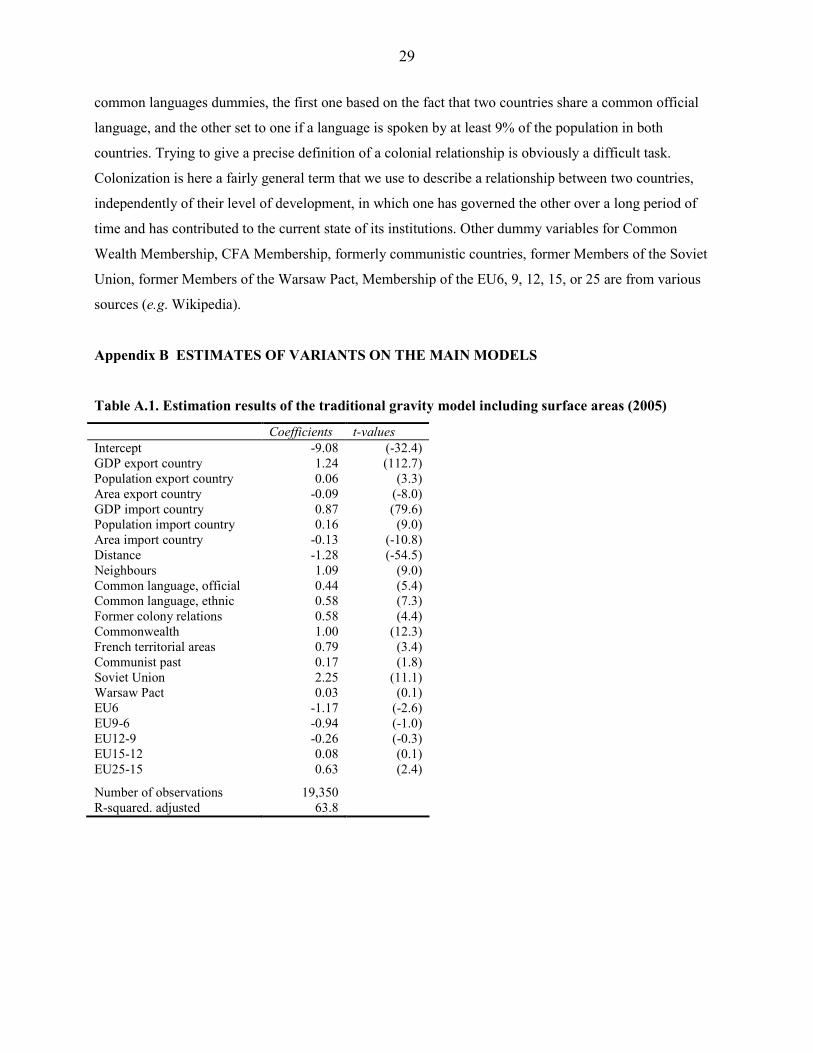
Appendix B ESTIMATES OF VARIANTS ON THE MAIN MODELS
Table A.1. Estimation results of the traditional gravity model including surface areas (2005)
Coefficients t-values
Intercept -9.08 (-32.4)
GDP export country 1.24 (112.7)
Population export country 0.06 (3.3)
Area export country -0.09 (-8.0)
GDP import country 0.87 (79.6)
Population import country 0.16 (9.0)
Area import country -0.13 (-10.8)
Distance -1.28 (-54.5)
Neighbours 1.09 (9.0)
Common language, official 0.44 (5.4)
Common language, ethnic 0.58 (7.3)
Former colony relations 0.58 (4.4)
Commonwealth 1.00 (12.3)
French territorial areas 0.79 (3.4)
Communist past 0.17 (1.8)
Soviet Union 2.25 (11.1)
Warsaw Pact 0.03 (0.1)
EU6 -1.17 (-2.6)
EU9-6 -0.94 (-1.0)
EU12-9 -0.26 (-0.3)
EU15-12 0.08 (0.1)
EU25-15 0.63 (2.4)
Number of observations 19,350
R-squared. adjusted 63.8
30
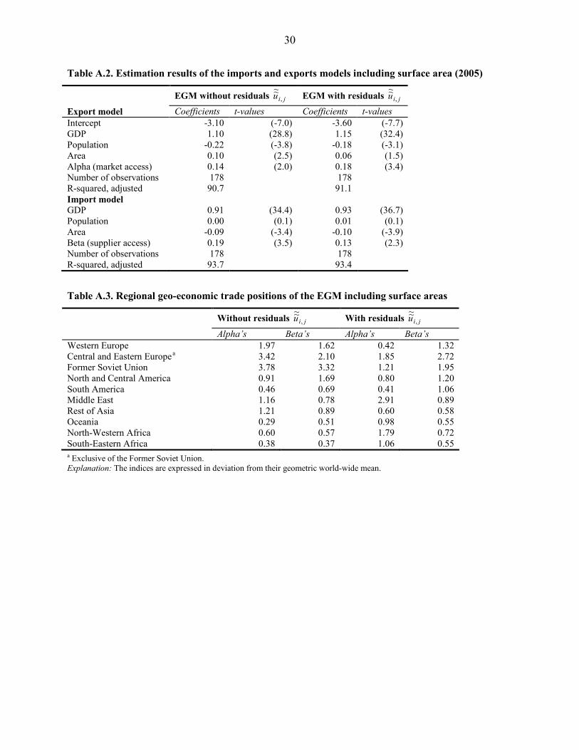
Table A.2. Estimation results of the imports and exports models including surface area (2005)
EGM without residuals jiu ,
~~ EGM with residuals jiu ,
~~
Export model Coefficients t-values Coefficients t-values
Intercept -3.10 (-7.0) -3.60 (-7.7)
GDP 1.10 (28.8) 1.15 (32.4)
Population -0.22 (-3.8) -0.18 (-3.1)
Area 0.10 (2.5) 0.06 (1.5)
Alpha (market access) 0.14 (2.0) 0.18 (3.4)
Number of observations 178 178
R-squared, adjusted 90.7 91.1
Import model
GDP 0.91 (34.4) 0.93 (36.7)
Population 0.00 (0.1) 0.01 (0.1)
Area -0.09 (-3.4) -0.10 (-3.9)
Beta (supplier access) 0.19 (3.5) 0.13 (2.3)
Number of observations 178 178
R-squared, adjusted 93.7 93.4
Table A.3. Regional geo-economic trade positions of the EGM including surface areas
Without residuals jiu ,
~~ With residuals jiu ,
~~
Alpha’s Beta’s Alpha’s Beta’s
Western Europe 1.97 1.62 0.42 1.32
Central and Eastern Europe a 3.42 2.10 1.85 2.72
Former Soviet Union 3.78 3.32 1.21 1.95
North and Central America 0.91 1.69 0.80 1.20
South America 0.46 0.69 0.41 1.06
Middle East 1.16 0.78 2.91 0.89
Rest of Asia 1.21 0.89 0.60 0.58
Oceania 0.29 0.51 0.98 0.55
North-Western Africa 0.60 0.57 1.79 0.72
South-Eastern Africa 0.38 0.37 1.06 0.55 a Exclusive of the Former Soviet Union.
Explanation: The indices are expressed in deviation from their geometric world-wide mean.


