
Time Consistency and the Duration of Government Debt:
A Signalling Theory of Quantitative Easing∗
Saroj Bhattarai
University of Texas-Austin
Gauti B. Eggertsson
Brown University and NBER
Bulat Gafarov†
Penn State
Abstract
We present a signalling theory of quantitative easing in which open market operations that change the
duration of outstanding nominal government debt affect the incentives of the central bank in determining
the real interest rate. In a time consistent (Markov-perfect) equilibrium of a sticky-price model with
coordinated monetary and fiscal policy, we show that shortening the duration of outstanding government
debt provides an incentive to the central bank to keep short-term real interest rates low in future in order
to avoid capital losses. In a liquidity trap situation then, where the current short-term nominal interest
rate is up against the zero lower bound, quantitative easing can be effective to fight deflation and a
negative output gap as it leads to lower real long-term interest rates by lowering future expected real
short-term interest rates. We show illustrative numerical examples that suggest that the benefits of
quantitative easing in a liquidity trap can be large in a way that is not fully captured by some recent
empirical studies.
JEL Classification: E31, E52, E58; E61; E63
Keywords: Time-consistent equilibrium; Duration of government debt; Quantitative easing; Liquidity
trap; Signalling; Zero lower bound; Sticky prices
∗Preliminary. We thank Oli Coibion, Mark Gertler, Andy Levin, Emi Nakamura, seminar participants at Emory University,University of Texas at Austin, and Brown University, and conference participants at NBER ME spring meeting, HKIMR/NewYork Fed conference on "Domestic and International Dimensions of Unconventional Monetary Policy," Society of EconomicDynamics Annual meeting, Mid-west Macro spring meeting, CEPR European Summer Symposium in International Macro-economics, Annual Conference on Computing and Finance, and NBER Japan Project Meeting for helpful comments andsuggestions. This version: Sept 2014.†Bhattarai: 2225 Speedway, Stop C3100, Austin, TX 78712; [email protected]. Eggertsson: Robinson Hall,
64 Waterman Street, Providence, RI 02912; [email protected]. Gafarov: Also affi liated with National ResearchUniversity Higher School of Economics; 605 Kern Building, University Park, PA 16802; [email protected].
1

1 Introduction
During the recent global financial crisis, central banks in many advanced economies such as the United
States engaged in various forms of “unconventional” monetary policy actions as the short-term interest
rate, the traditional policy instrument, was up against the zero lower bound. One form of such policy
actions involved changes in the size and/or composition of the central bank’s balance sheet. In particular,
the Federal Reserve in the United States carried out several large scale purchases of assets in recent years,
a program often referred to collectively as Large Scale Asset Purchases (LSAPs). A considerable part of
LSAPs involved buying long term government bonds, or “quantitative easing,”a naming convention we use
here.
What is quantitative easing? It is when the government buys long-term government debt with money.
Since the nominal interest rate was zero in recent years when this policy was implemented in the United
States, it makes no difference if this was done by printing money (or more precisely bank reserves) or by
issuing short-term government debt: both are government issued papers that yield a zero interest rate. From
the perspective of the government as a whole, at least, quantitative easing at zero nominal interest rates can
then simply be thought of as shortening the maturity of outstanding government debt.1 The government is
simply exchanging longer term liabilities in the hands of the public with shorter term ones.
The main goal of quantitative easing in the United States was to reduce long-term interest rates, even
when the short-term nominal interest rate could not be reduced further, and thereby, stimulate the economy.
Indeed, several empirical studies find evidence of reduction in long-term interest rates following these policy
interventions by the Federal Reserve. For example, Gagnon et al (2011) estimate that the 2009 program
that involved buying various types of debt worth $1.75 trillion reduced long-term interest rates by 58 basis
points while Krishnamurthy and Vissing-Jorgensen (2011) estimate that the 2010 program that involved
buying long-term government debt worth $600 billion reduced long-term interest rates by 33 basis points.
In addition, Hamilton and Wu (2012), Swanson and Williams (2013), and Bauer and Rudebusch (2013) also
find similar effects on long-term interest rates.2
From a theoretical perspective however, the effect of such policy is not obvious since open market oper-
ations of this kind are neutral (or irrelevant) in standard macroeconomic models. This was pointed out first
in a well-known contribution by Wallace (1981) and further extended by Eggertsson and Woodford (2003)
to a model with sticky prices and an explicit zero lower bound on nominal interest rates. These papers
showed how absent some restrictions in asset trade that prevent arbitrage, a change in the relative supplies
of various assets in the hands of the private sector has no effect on equilibrium quantities and asset prices
in prototypical macroeconomic models.
For this reason, some papers have recently incorporated frictions such as participation constraints due
to “preferred habitat”motives in order to make assets of different maturities imperfect substitutes. This
in turn negates the neutrality of open market operations as in such an environment, quantitative easing
can reduce long-term interest rates because it decreases the risk-premium. For example, Chen, Curdia, and
Ferrero (2012) augment a quantitative sticky price model with such segmented market frictions and show
that purchases of long-term bonds by the central bank can reduce long-term interest rates by decreasing
the risk-premium. They nevertheless find the effects to be fairly modest: based on their estimated model,
1 Indeed our model will be one where we will consider a consolidated government budget constraint and joint conduct ofoptimal monetary and tax policy.
2Note however that empirical studies typically measure nominal interest rates, while theoretically, it is the ability to influencereal interest rates that matter. This issue is quite important and we emphasize it in detail later.
2

they find that a $600 billion reduction in outstanding long-term debt, along with a commitment to keep
short-term interest rates at zero for 4 quarters, increases inflation by 3 basis points (annualized) and GDP
growth by 0.13% (annualized).
As Woodford (2012) argues however (building on Eggertsson and Woodford (2003)), quantitative easing
need not be effective only because it reduces risk premiums. It can also reduce long-term interest rates if
such policy intervention signals to the private sector that the central bank will keep the short-term interest
rates low once the zero lower bound is no longer a constraint in the future. In fact, arguably, much of the
findings of the empirical literature on reduction of long-term interest rates due to quantitative easing can
be attributed to expectations of low future short-term interest rates. Indeed, Krishnamurthy and Vissing-
Jorgensen (2011) and Bauer and Rudebusch (2013) find evidence in support of this channel in their study
of the various quantitative easing programs.3
Our contribution is to provide a formal theoretical model of such a “signalling” role of quantitative
easing in a standard general equilibrium sticky price model.4 In particular, we consider coordinated optimal
monetary and fiscal policy under discretion and show that in a Markov-perfect (time-consistent) equilibrium,
shortening the duration of outstanding government debt provides an incentive to the central bank to keep
the short-term real interest rate low in the future. This constitutes optimal policy under discretion because
it avoids capital losses on the government’s balance sheet, which if realized, would entail raising taxes that
are costly in the model. The key intuition for this result is that if the government holds larger amount of
short-term debt then current real short term rate directly affects the cost of rolling the debt over period by
period, while the cost of rolling over long-term debt is not affected as strongly period by period (since the
interest rate on that debt is predetermined at the time the policy is set). This implies that shortening the
maturity of outstanding debt increases the incentive of the government to keep real rates low.
In a liquidity trap situation, where the current short-term nominal interest rate is up against the zero
lower bound and the economy suffers from deflation and a large negative output gap, it is well known that
signalling about future policy can be very effective. For example, Krugman (1998) emphasizes the importance
of raising inflation expectations and Eggertsson and Woodford (2003) emphasize the commitment to lower
future short-term nominal interest rate and allowing output to overshoot its steady state level. But are
these type of commitments credible? In fact, it is well-understood that commitment to future expansionary
policy at the zero lower bound is diffi cult due to time-inconsistency problems. While the public understands
the benefits today of committing to lower future real interest rates, it also appreciates the government’s
incentive in the future to renege on these promises once the economy has recovered (this leads to the so
called “deflation bias”developed in Eggertsson (2006)). Our main result, then, is that quantitative easing,
or shortening the duration of government debt, makes promises of expansionary future policy “credible”
because it provides an incentive to the central bank to keep short-term real interest rates low in future to
avoid balance sheet losses. This mitigates the extent of deflation and negative output gap that would occur
otherwise in the Markov-perfect equilibrium.5
3Woodford (2012) makes a similar argument regarding empirical evidence on most recent balance sheet policies by theFederal Reserve.
4Gagnon et al (2011) label this role played by the expected path of future short-term interest rates as a “signalling”role forquantitative easing. In the literature on central bank intervention in foreign exchange markets, this term has been used oftenand appears to have been first coined by Mussa (1981) to discuss how foreign exchange interventions might be used to signalfuture changes in monetary policy.
5Jeanne and Svensson (2007) assume net worth concerns on the part of the central bank directly and show how buyingforeign exchange is useful during a liquidity trap as it commits the central bank to not appreciating the exchange rate infuture (since doing so would entail capital losses on the central bank’s balance sheet). Berriel, Bhattarai, and Mendes (2013)show that buying long-term bonds acts as a commitment device for the same reason. The main difference in this paper is theconsideration of joint conduct of monetary and fiscal policy along with a welfare-theoretic loss function for the government.
3

In our calibrated model, we show numerical experiments in which these effects of quantitative easing
can be very large. For example, with government debt maturity of 16 quarters, we calibrate the size of
the negative demand shock (that makes the zero lower bound binding) such that output drops by 10% and
(annualized) inflation by 2%. In such a case, reducing the duration of government debt by 7 months decreases
(annualized) deflation and the negative effect on output by 95.4 and 140 basis points respectively.6 This
suggests that the signalling channel may explain all the effects of quantitative easing found in the empirical
literature. In addition, we show that if the duration were to be reduced by 20.6 months, that is triple the
size of our baseline experiment for quantitative easing, the negative output gap at the zero lower bound
would be completely eliminated.
Before presenting the model we want to clarify an important element of our analysis. A key to un-
derstanding optimal policy in the New Keynesian model at the zero bound is that it involves committing
to lower future short-term real interest rates.7 The short term real interest rate is the difference between
future short-term nominal interest rate and expected inflation. A lower short-term real interest rate can be
achieved by either a lower future short-term nominal interest rate or higher future expected inflation. A
commitment of this kind will under some parameterization of the model be achieved via higher expected
inflation and higher future short-term nominal interest rates —even if the difference between the two (the
real rate) is going down. An implication of this is that a successful policy of quantitative easing aimed at
lowering long-term real interest rate may involve an increase in expected future nominal interest rates and
therefore, an increase in long-term nominal rates at the zero lower bound. This is relevant because some
empirical analyses of the effect of quantitative easing focus only on long-term nominal interest rates, which
our analysis suggests is not a suffi cient statistic. Even if long-term nominal interest rate decline very little
in response to quantitative easing, or even if they increase, this does not by itself suggest that the policy is
ineffective, as long as the real interest rate is declining.
Finally, while the paper connects with work related to the zero lower bound in models with nominal
rigidities, it also is related to the theoretical literature on how the maturity structure of debt can be manip-
ulated to eliminate the dynamic inconsistency found in many monetary models (in particular the “inflation
bias”) such as Lucas and Stokey (1983), Persson, Persson, and Svensson (1987 and 2006), and Alvarez,
Kehoe, and Neumeyer (2004). While the focus of these papers is generally on policies that eliminates the
incentive to inflate, the inflation bias, (and thus generally imply a lengthening of the duration of government
debt relative to one-period debt), our application can be thought of as precisely the opposite, that is, the
maturity structure of debt is made shorter to solve the “deflation bias.”
2 The Model
2.1 Private sector
The model is a standard general equilibrium sticky-price closed economy set-up with an output cost of
taxation, along the lines of Eggertsson (2006). The government conducts coordinated monetary and fiscal
policy under discretion. While it may seem like a distraction to write out the fully non-linear model and
define the equilibrium in that context, as we will later on analyze a linear quadratic version of this model,
6We use these numbers for illustration based on estimates in Chadha, Turner, and Zampoli (2013), which suggest that theaverage maturity of treasury debt held outside the Federal Reserve was around 4 years in the last 10 years and that recentFederal Reserve balance sheet policies reduced the maturity by around 7 months.
7Werning (2012) makes a related point regarding the ultimate goal of optimal policy as one of generating an output boomonce the trap is over.
4
this is useful for two reasons. First, we will formally show that the linearized first-order conditions of the
government’s original non-linear problem are the same as in our linear quadratic model (and this in general
need not be the case, see e.g. Eggertsson (2006)). Second, the non-linear version of the problem will be
important once we allow for fully time-varying duration of government debt, where the linear quadratic
approximation is no longer valid.
The main difference in the model from the literature is the introduction of long-term government debt.
A representative household maximizes expected discounted utility over the infinite horizon
Et
∞∑t=0
βtUt = Et
∞∑t=0
βt [u (Ct) + g (Gt)− v(ht))] ξt (1)
where β is the discount factor, Ct is household consumption of the composite final good, Gt is government
consumption of the composite final good, ht is quantity supplied of labor of type i, and ξt is a shock. Etis the mathematical expectation operator conditional on period-t information, u (.) is concave and strictly
increasing in Ct, g (.) is concave and strictly increasing in Gt, and v (.) is increasing and convex in ht.8
The composite final good is an aggregate of a continuum of varieties indexed by i, Ct =∫ 1
0
[ct(i)
ε−1ε di
] εε−1
,
where ε > 1 is the elasticity of substitution among the varieties. The optimal price index for the composite
final good is given by Pt =[∫ 1
0pt(i)
1−εdi] 11−ε
, where pt(i) is the price of the variety i. The demand for
the individual varieties is then given by ct(i)Ct
=(pt(i)Pt
)−ε. Finally, Gt is defined analogously to Ct and so
we omit detailed description of government spending.
The household is subject to a sequence of flow budget constraints
PtCt +BSt + StBt + Et{Qt,t+1At+1} ≤ ntht + (1 + it−1)BSt−1 + (1 + ρSt)Bt−1 +At − PtTt +
∫ 1
0Zt(i)di (2)
where nt is nominal wage, Zt(i) is nominal profit of firm i, BSt is the household’s holding of one-period
risk-less nominal government bond at the beginning of period t + 1, Bt is a perpetuity bond, St its price,
and ρ its decay factor (further described below). At+1 is the value of the complete set of state-contingent
securities at the beginning of period t+ 1 and Qt,t+1 is the stochastic discount factor between periods t and
t+1 that is used to value random nominal income in period t+1 in monetary units at date t.9 Finally, it−1 is
the nominal interest rate on government bond holdings at the beginning of period t and Tt is government
taxes.
The way we introduce long term bonds into the model is to assume that government debt not only
takes the form of a one period riskfree debt, BSt , but that the government also issues a perpetuity in period
t which pays ρj dollars j + 1 periods later, for each j ≥ 0 and some decay factor 0 ≤ ρ < β−1.10 St is
the price of the perpetuity nominal bond which depends on the decay factor ρ. The main convenience of
introducing long term bond in this way is that we can consider government debt of arbitrary duration. For
example, a value of ρ = 0 implies that this bond is simply a short-term bond while ρ = 1 corresponds to
a classic console bond. More generally, in an environment with stable prices, the duration of this bond is
(1− βρ)−1. Thus, this simple assumption allows us to explore a change in the duration of government debt
in a transparent way. The appendix contains details on why the budget constraint takes the form (2). In
particular, the modelling of long-term bond in this way admits a simple recursive formulation of the price
of old government bonds.
8We abstract from money in the model and are thus directly considering the “cash-less limit.”9The household is subject to a standard no-Ponzi game condition.10We follow Woodford (2001).
5
For now, observe that we treat ρ as a constant. We will explore a one-time reduction in this duration as
a main "comparative static" of interest. In other words, a reduction in ρ answers the question: What does
a permanent reduction in the maturity of government debt do? Toward the end of the paper, however, we
will extend the analysis so that ρ becomes a time varying choice variable ρt. The main reason for our initial
benchmark assumption is simplicity (and the fact that we get a clean comparative static). But perhaps
more importantly, we will see later that a one-time reduction in ρ (in a liquidity trap) turns out to be a
reasonably good approximation in our model because ρt is close to a random walk under optimal policy
under discretion at a positive interest rate.
The maximization problem of the household is now entirely standard, with the additional feature of the
portfolio choice between long and short term bonds.11 Let us now turn to the firm side of the model.
There is a continuum of monopolistically competitive firms indexed by i. Each firm produces a variety
i according to the production function that is linear in labor yt(i) = ht(i). As in Rotemberg (1983), firms
face a cost of changing prices given by d(
p(i)pt−1(i)
). This adjustment cost makes the firm’s pricing problem
dynamic. The demand function for variety i is given by
yt(i)
Yt=
(pt(i)
Pt
)−ε(3)
where Yt is total demand for goods. The firm maximizes expected discounted profits
Et
∞∑s=0
Qt,t+sZt+s(i) (4)
where the period profits Zt(i) are given by
Zt(i) =
[(1 + s)Ytpt(i)
1−εP εt − nt(i)Ytpt(i)−εP εt − d(
pt(i)
pt−1(i)
)Pt
]where s is a production subsidy which we will set to eliminate the steady state distortion of monopolistic
competition as is common in the literature.12
We can now write down the necessary conditions for equilibrium that arise from the maximization
problems of the private sector described above. We focus on a symmetric equilibria where all firms charge
the same price and produce the same amount of output. Note that these conditions hold for any government
policy.
The households optimality conditions are given by
vh (ht)
uC (Ct)=ntPt
(5)
1
1 + it= Et
[βuC(Ct+1)ξt+1
uC(Ct)ξtΠ−1t+1
](6)
St = Et
[βuC(Ct+1)ξt+1
uCCt)ξtΠ−1t+1 (1 + ρSt+1)
](7)
11The problem of the household is thus to choose {Ct+s, ht+s(i), BSt+s, Bt+s, At+s} to maximize (1) subjectto a sequence of flow budget constraints given by (2), while taking as exogenously given initial wealth and{Pt+s,nt+s(i), it+s, St+s(ρ), Qt,t+s, ξt+s, Zt+s(i), Tt+s}.12The problem of the firm is thus to choose {pt+s(i)} to maximize (4), while taking as exogenously given{Pt+s,Yt+s, nt+s(i), Qt,t+s, ξt+s}
6
where Πt = PtPt−1
is gross inflation.13 The firm’s optimality condition from price-setting is given by
εYt [uC (Ct)− vy(Yt)] ξt + uC(Ct)ξtd′ (Πt) Πt = Et [βuCCt+1)ξt+1d
′ (Πt+1) Πt+1] (8)
where with some abuse of notion we have replaced vh with vy since in a symmetric equilibrium ht(i) =
yt(i) = Yt.
2.2 Government
There is an output cost of taxation (for example, as in Barro (1979)) captured by the function s(Tt−T ) where
T is the steady-state level of taxes. Thus, in steady-state, there is no tax cost. Total government spending
is then given by
Ft = Gt + s(Tt − T )
where Gt is aggregate government consumption of the composite final good defined before.
It remains to write down the (consolidated) flow budget constraint of the government. Note that the
government issues both a one-period bond BSt and the perpetuity Bt. We can write the flow budget constraint
as
BSt + StBt = (1 + it−1)Bt−1 + (1 + ρSt)Bt−1 + Pt (Ft − Tt) .
Next, we assume that the one-period bond is in net-zero supply (i.e. BSt = 0, which makes clear that we
only introduce this bond explicitly as the risk free short term nominal rate is the key policy instrument of
monetary policy), and write the budget constraint in real terms as
Stbt = (1 + ρSt) bt−1Π−1t + (Ft − Tt) (9)
where bt = BtPt. We now define fiscal policy as the choice of Tt, Ft , and bt. For simplicity, we will from now
on suppose that total government spending is constant so that Ft = F. Monetary policy is the choice of it.
We simply impose the zero bound constraint on the setting of monetary policy so that14
it ≥ 0. (10)
2.3 Private sector equilibrium
The goods market clearing condition gives the overall resource constraint as
Yt = Ct + Ft + d (Πt) . (11)
We can then define the private sector equilibrium, that is the set of possible equilibria that are consistent
with household and firm maximization and the technological constraints of the model. A private sector
equilibrium is a collection of stochastic processes {Yt+s, Ct+s, bt+s, St+s, Πt+s, it+s, Qt,t+s, Tt+s, Ft+s,
Gt+s} for s ≥ 0 that satisfy equations (5)-(7), (8), (9), and (11), for each s ≥ 0, given bt−1 and an
exogenous stochastic process for {ξt+s}. To determine the set of possible equilibria in the model, we nowneed to be explicit about how policy is determined.
13We may also append a standard transversality condition as a part of these conditions or a natural borrowing limit.14This bound can be explicitly derived in a variety of environment, see e.g. Eggertsson and Woodford (2003).
7

3 Markov-perfect Equilibrium
We characterize a Markov-perfect (time-consistent) Equilibrium in which the government cannot commit
and acts with discretion every period.15 In particular, we consider coordinated monetary and fiscal policy,
where the central bank and the treasury conduct optimal monetary and fiscal policy under discretion. A
key assumption in a Markov-perfect Equilibrium is that government policy cannot commit to the actions
for the future government. Following Lucas and Stokey (1983), however, we suppose that the government is
able to commit to paying back the nominal value of its debt.16 The only way the government can influence
future governments, then, is via any endogenous state variables that may enter the private sector equilibrium
conditions. Before writing up the problem of the government, it is therefore necessary to write the system
in a way that makes clear what are the endogenous state variables of the game we study.
Define the expectation variables fEt , gEt , and h
Et . The necessary and suffi cient condition for a private
sector equilibrium is now that the variables {Yt, Ct, bt, St, Πt, it, Tt} satisfy: (a) the following conditions
St(ρ)bt = (1 + ρSt(ρ)) bt−1Π−1t + (F − Tt) (12)
1 + it =uC (Ct) ξtβfEt
, it ≥ 0 (13)
St(ρ) =1
uC (Ct) ξtβgEt (14)
βhEt = εYt
[ε− 1
εuC (Ct) ξt − vy (Yt) ξt
]+ uC (Ct) ξtd
′ (Πt) Πt (15)
Yt = Ct + F + d (Πt) (16)
given bt−1 and the expectations fEt , gEt , and h
Et ; (b) expectations are rational so that
fEt = Et[uC (Ct+1) ξt+1Π−1
t+1
](17)
gEt = Et[uC (Ct+1) ξt+1Π−1
t+1 (1 + ρSt+1(ρ))]
(18)
hEt = Et [uC (Ct+1) ξt+1d′ (Πt+1) Πt+1] . (19)
Note that the possible private sector equilibrium defined above depends only on the endogenous state
variable bt−1 and shocks ξt. Given that the government cannot commit to future policy (apart from through
the endogenous state variable), a Markov-perfect Equilibrium then requires that the expectations fEt , gEt ,and
hEt are only a function of these two state variables, i.e, we can define the expectation functions
fEt = fE(bt, ξt) (20)
gEt = gE(bt, ξt) (21)
hEt = hE(bt, ξt). (22)
We can now write the discretionary government’s optimization problem as a dynamic programming
problem
V (bt−1, ξt) = maxit,Tt
[U (.) + βEtV (bt, ξt+1)] (23)
15See Maskin and Tirole (2001) for a formal definition of the Markov-perfect equilibrium.16One could model this more explicitly by assuming that the cost of outright default is arbitrarily high.
8
subject to the private sector equilibrium conditions (12)-(16) and the expectation functions (20)-(22). Note
that in equilibrium, the expectation functions satisfy the rational expectation restrictions (17)-(19). Here,
U (.) is the utility function of the household in (1) and V (.) is the value function.17 The detailed formulation
of this maximization problem and the associated first-order necessary conditions, as well as their linear
approximation, are provided in the appendix.18
4 Linear-quadratic approach
Rather than studying the fully non-linear policy problem, we will instead do a linear-quadratic approximation
of the policy problem. The main reason for this approach is that it clarifies the interpretation of our result,
and connects more closely to some of the earlier literature. As we will see shortly (Proposition 1), however,
this approach yields the same solution as if we would have approximated directly the non-linear first-order
conditions of the problem (23). When moving to time-varying ρ, however, a linear quadratic approximation
will no longer be valid, in which case we will only rely on the fully non-linear statement of the government’s
decision problem.
We approximate our model around an effi cient non-stochastic steady-state with zero inflation.19 More-
over, there are no tax collection costs in steady-state20 . Thus, there is a non-zero steady-state level of debt.21
In steady-state, we assume that there is some fixed total market-value of public debt Sb = Γ. Then, the
following relationships hold
1 + i = β−1, S =β
1− ρβ , b =1− ρββ
Γ and T = F +1− ββ
Γ.
We log-linearize the private sector equilibrium conditions around the steady state above to get the relation-
ships
Yt = EtYt+1 − σ(ıt − Etπt+1 − ret ) (24)
πt = κYt + βEtπt+1 (25)
bt = β−1bt−1 − β−1πt − (1− ρ)St − ψTt (26)
St = −ıt + ρβEtSt+1 (27)
where κ and σ are a function of structural model parameters that do not depend upon ρ and ret is the
effi cient rate of interest that is a function of the shock ξt.22 The coeffi cient ψ ≡ TΓis also independent of ρ
in our experiment.23
Here, (24) is the linearized household Euler equation, (25) is the linearized Phillips curve, (26) is the
linearized government budget constraint, and (27) is the linearized forward-looking asset-pricing condition.24
17Using compact notation, note that we can write the utility function as [u (Ct) + g (F − s(Tt − T ))− v (Yt)]ξt.18Note here that we assume that the government and the private-sector move simultaneously.19Variables without a t subscript denote a variable in steady state. Note that output is going to be at the effi cient level in
steady state because of the assumption of the production subsidy (appropriately chosen) we have made before.20We can think of this as being due to a limited set of lump sum taxation.21The steady-state is effi cient even with non-zero steady-state debt because of our assumption that taxes do not entail output
loss in steady-state.22The details of the derivation are in the appendix.23Since we are thinking of changes in ρ in our experiment as exchanging short bonds with long bonds — effectively reduc-
ing/increasing ρ —this interpretation would imply that total value of debt in steady-state — Γ—should remain unchanged.24Variables with hats denote log-deviations from steady state except for the nominal interest rate, which is given as ıt = it−i
1+i.
Since in the non-stochastic steady state with zero inflation, 1+ i = 1β, this means that the zero lower bound on nominal interest
9
(24) and (25) are standard relationships depicting how current output depends on expected future output
and the current real interest rate gap and how current inflation depends on expected future inflation and
the current output respectively.25
(26) shows that since debt is nominal, its real value is decreased by inflation. Higher taxes also reduce the
debt burden. Moreover, an increase in the price of the perpetuity bond decreases the real value of debt, with
the effect depending on the duration of debt: longer the duration, lower is the effect of the bond price on
debt. Finally, (27) shows that the price of the perpetuity bond is determined by (the negative of) expected
present value of future short-term interest rates. Hence, lower current or future short-term nominal interest
rate will increase the price of the perpetuity bond. Note that when ρ = 0, all debt is of one-period duration
and (26) reduces to the standard linearized government budget constraint while (27) reduces to St = −ıt.26
A second-order approximation of household utility around the effi cient non-stochastic steady state gives
Ut = −[λππ
2t + Y 2
t + λT T2t
](28)
where λπ and λT are a function of structural model parameters.27 Compared to the standard loss-function
in models with sticky prices that contains inflation and output, (28) features losses that arise from output
costs of taxation outside of steady-state.
To analyze optimal policy under discretion in the linear-quadratic framework we once again maximize
utility, subject the now linear private sector equilibrium conditions, taking into account that the expectation
are functions of the state variables of the game. In the linear system, the exogenous state is now summarized
with ret while the endogenous state variable is once again bt−1.Moreover, the expectation variables appearing
in the system are now EtYt+1, EtSt+1, and Etπt+1. Accordingly, we will define the game in terms of the state
variables (ret , bt−1) and the government now takes as given the expectation functions Y E(bt, ret ), S
E(bt, ret ),
and πE(bt, ret ).
The discretionary government’s optimization problem can then be written recursively as a linear-quadratic
dynamic programming problem
V (bt−1, ret ) = min[λππ
2t + Y 2
t + λT T2t + βEtV (bt, r
et+1)]
s.t.
Yt = Y E(bt, ret )− σ(ıt − πE(bt, r
et )− ret )
πt = κYt + βπE(bt, ret )
bt = β−1bt−1 − β−1πt − (1− ρ)St − ψTt
St = −ıt + ρβSE(bt, ret )
Observe that once again, in equilibrium, the expectation functions need to satisfy the rational expectations
restrictions that EtYt+1 = Y E(bt, ret ), EtSt+1 = SE(bt, r
et ), and Etπt+1 = πE(bt, r
et ).
We prove in the proposition below that this linear-quadratic approach gives identical linear optimality
rates imposes the following bound on ıt : ıt ≥ − (1− β) .25We write directly in terms of output rather than the output gap since we will not be considering shocks that perturb the
effi cient level of output in the model.26 It is important to point out one techical detail in this case. The interpretation in this case of bt is that it is the real value
of the debt inclusive of the interest rate payment to be paid next period, that is, if all debt were one period bt = (1 + it)BStPt.
27The details of the derivation are in the appendix. In particular, λπ = εk.
10
conditions as the one obtained by linearizing the non-linear optimality conditions of the original non-linear
government maximization problem that we described above. This provides the formal justification of our
simplified approach.
Proposition 1 The linearized dynamic system of the non-linear Markov Perfect Equilibrium is equivalent
to the linear dynamic system of the linear-quadratic Markov Perfect Equilibrium.
Proof. In Appendix.
4.1 Solution at positive interest rates
The complication in solving a Markov-perfect Equilibrium is that we do not know the unknown expectation
functions πE , Y E , and SE . To solve this, we use the method of undetermined coeffi cients. Provided that
the expectation functions are differentiable, the solution of the model is of the form
πt = πbbt−1 + πrret , Yt = Ybbt−1 + Yrr
et , St = Sbbt−1 + Srr
et , (29)
ıt = ibbt−1 + irret , Tt = Tbbt−1 + Trr
et , and bt = bbbt−1 + brr
et
where πb, Yb, Sb, ib, bb, Tb, πr, Yr, Sr, ir, br, and Tr are unknown coeffi cients to be determined. We make
the assumption that the exogenous process ret satisfies Etret+1 = ρrr
et where 0 < ρr < 1. Then (29) implies
that the expectations are given by
Etπt+1 = πbbt + πrρrret , EtYt+1 = Ybbt + Yrρrr
et , and EtSt+1 = Sbbt + Srρrr
et . (30)
We can then formulate the Lagrangian of the government problem. We substitute out for the expectation
function using (30) and suppress the shock for simplicity
Lt =1
2(λππ
2t + Y 2
t + λT T2t ) + βEtV (bt, r
et+1)
+ φ1t[Yt − Ybbt + σıt − σπbbt] + φ2t[πt − κYt − βπbbt]
+ φ3t[bt − β−1bt−1 + β−1πt + (1− ρ)St + ψTt] + φ4t[St + ıt − ρβSbbt].
For now, we are not analyzing the effects of the shock, and hence not carrying around πr, Yr, Sr, ir, br, and
Tr since our key area of interest at this state is not the effect of the shock at positive interest rates. Instead,
we will start focusing on the shock once the zero bound becomes binding.
The associated first order necessary conditions of the Lagrangian problem above and the envelope condi-
tion of the minimization problem of the government above are provided in the appendix. Our first substan-
tiative result is that the equilibrium conditions can be simplified, in particular by eliminating the Lagrange
multipliers φ1t − φ4t, to get
λππt + κ−1Yt = [κ−1 (1− ρ)σ−1 + β−1]1
ψλT Tt (31)
[1− βπbκ−1 (1− ρ)σ−1 − (Yb + σπb) (1− ρ)σ−1 + ρβSb(1− ρ)]Tt = − (ψ)λ−1T βπbκ
−1Yt + EtTt+1 (32)
which along with (24)-(27) define the equilibrium in the approximated economy. The final step to computing
the solution is then to plug in the conjectured solution and to match coeffi cients on various variables in (24)-
11
(27), (31), and (32), along with the requirement that expectation are rational, to determine πb, Yb, Sb, ib,
bb, and Tb. The details of this step are in the appendix.
The most important relationships emerging from our analysis are captured by (31) and (32). (31) is
the so called “targeting rule” of our model. That represents the equilibrium (static) relationship among
the three target variables πt, Yt, and Tt that emerges from the optimization problem of the government.
(31) thus captures how target variables are related in equilibrium as governed both by the weights they
are assigned in the loss function (λπ and λT ) as well as the trade-offs among them as given by the private
sector equilibrium conditions (κ−1 and [κ−1 (1− ρ)σ−1 +β−1] 1ψ ). Note in particular that κ
−1 represents the
trade-off between πt and Yt as given by (25) while [κ−1 (1− ρ)σ−1 +β−1] 1ψ represents the trade-off between
πt and Yt vs. Tt as given by the combination of (24), (25), and (26).
(32) is another optimality condition characterizing the Markov-perfect equilibrium and represents the
“tax-smoothing objective”of the government. In contrast to similar expressions following the work of Barro
(1979), which would lead to taxes being a martingale, output appears in (32) because of sticky-prices, which
makes output endogenous. Finally, because of the dynamic nature of (32), as opposed to (31), the unknown
coeffi cients that are critical for expectations of variables, πb, Yb, and Sb, appear in (32). As we shall see
—and this is again in contrast to the classic tax smoothing result in which debt is a random walk — the
government will in general have an incentive to pay down public debt if it is above steady-state due to
strategic reasons.
4.1.1 Debt dynamics, inflation, and interest rates
Let us first consider the most basic exercise to clarify the logic of the government’s problem. How do the
dynamics of the model look like in the absence of shocks when the only difference from steady state is that
there is some initial value of debt with some fixed value of debt duration? To do this exercise we calibrate
the model as follows. The parameter values we pick are given in Table 1. Following Eggertsson (2006), we
choose our baseline parameters as follows: β = 0.99, σ = 1, κ = 0.02, and ε = 8. For the steady-state level
of debt-to-taxes, bST = ΓT , we use data from the Federal Reserve Bank of Dallas to get the long-run average
of market value of debt over output ( bSY ) and NIPA data to estimate the ratio of taxes over output ( TY ).
This gives us the value bST = Γ
T = 7.2. There is no direct counterpart to λT = s′′
φ+σ−1 in the data, and hence
we will experiment with several values and discuss our choices further below. For now, we set it at 0.8,
so that tax distortions obtain less weight than output in the objective of the government. The parameter
ρ is chosen to get a (baseline) duration of debt of 16 quarters. We pick this value based on estimates in
Chadha, Turner, and Zampoli (2013) which suggest that the average maturity of treasury debt held outside
the Federal Reserve was around 4 years in the last 10 years
Figure (1) shows the dynamics of the endogenous variables in the model for an initial value of debt that
is 30 percent above the steady state debt in the model.28 We see that if debt is above steady state, it is
paid over time back to steady state. For our baseline duration of 16 quarters (solid line), the half-life of
debt repayment is about 30 quarters. Note that in this transition for this parameterization, inflation is
about 1 percent above steady state. Importantly, in the transition phase, we see that the real interest rate
is below its steady state. As a consequence, output is also above its steady state value. Note that this
result is in contrast to the classic Barro tax smoothing result whereby debt follows a random walk. The
reason for this is that debt creates an incentive to create inflation for a discretionary government as further
28This is consistent with data from the Federal Reserve Bank of Dallas which suggests that at 2008:IV, government debt wasaround 30 percent above the steady state.
12
described below. By paying down debt back to steady state, the government thus eliminates this incentive
and achieves better outcomes.
The figure illustrates that for a given maturity of government debt, debt is inflationary and implies lower
future real interest rate until a new steady state is reached. What is the logic for this result? Perhaps the
best way to understand the logic is by inspecting the government budget constraint (26). Recall that debt
issued in nominal terms, although in the budget constraint we have rewritten it in terms of bt =BtPt−bb
.
This implies that for a given outstanding debt bt−1, any actual inflation will reduce the real value of the
outstanding debt. Accordingly we have the term β−1πt term in the budget constraint which reflects this
inflation incentive. As the literature has stressed in the past (see e.g. Calvo and Guidotti (1990 and 1992)),
if prices are flexible then this will reduce actual debt in equilibrium only if the inflation is unanticipated.
The reason for this is that otherwise anticipated inflation will be reflected one-to-one in the interest rate
paid on the debt.
Apart from the inventive to depreciate the real value of the deb via inflation, there is a second force
at work in our model. In our model, the government is not only able to affect the price level, it can also
have an effect on the real interest rate. Hence we see that in Figure 1 the real interest rate is below steady
state during the entire transition path back to steady state. This will reduce the real interest rate payment
the government needs to pay on debt — in contrast to the classic literature with flexible prices where the
(ex-ante) real interest rate is exogenous. Intuitively, it may be most straight forward to see this force at
work by simplifying the model down to the case in which ρ = 0. In that case, the budget constraint of the
government can be written as
bt = β−1bt−1 − β−1πt + ıt − ψTt
and now bt is the real value of one period risk-free nominal debt in period t which is inclusive of interest
paid (to relate to our prevision notation in 2 then when ρ = 0 we have bt = BtPt
=(1+it)B
St
Ptwhere BSt was
the one period government debt that did not include interest payment). This expression makes clear that
while πt has a direct effect by depreciating the real value of government debt, the government has another
important margin by which it can influence its debt burden. The term ıt reflects the cost or rolling-over-cost
of the one-period debt. In particular, we see that if the interest rate is low, then the cost of rolling over
debt is smaller. This latter mechanism will be critical when considering the effects of varying debt maturity
since its force is highly depending on the value of ρ.
4.1.2 The role of duration of debt
We now consider how reducing the value of ρ affects the transition dynamics from last section. As noted
before, our main interest for this is that a natural interpretation of quantitative easing is that it corresponds
to a reduction in ρ as in our model, as the duration of debt is given by (1−βρ)−1. As Figure (1) reveals, where
we consider a reduction in duration from 4 years to 3.42 and 2 years (dotted and dashed lines respectively),
this increases inflation in equilibrium considerably, but also reduce the real rate further. Similarly, we see
that the debt is now paid down at a faster clip, a point we will return to.
To obtain some intuition for this result, let us again write out the budget constraint, this time substituting
out for St to obtain
bt = β−1bt−1 − β−1πt + (1− ρ)[ıt − ρβSE(bt, ret )]− ψTt (33)
We observe here that the rollover interest rate is now multiplied by the term (1− ρ). Intuitively then, if a
larger part of government debt is held with long maturity, the short-term rollover rate matters less, as the
13
term of the loans are to a greater extent predetermined. Hence, the incentive of the government to lower
the short-term interest rate are reduced.
4.1.3 Real interest rate incentives and duration of outstanding debt
How does the duration of debt affect the real interest rate incentives of the central bank? The effect on the
real interest rate of lower duration is at the heart of the matter because what influences output is eventually
the real interest rate and the aim in a zero lower bound situation is precisely to be able to decrease the
short-term real interest rate (today and in future) even when the current short-term nominal interest rate
is stuck at zero. That is, we are interested in the properties of
rt = ıt − Etπt+1 = (ib − πbbb) bt−1 = rbbt−1
where rt is the short-term real interest rate. This is important because in a liquidity trap situation, as is
well-known, decreasing future real interest rate is key to mitigating negative effects on output, and so, if rbdepends negatively on duration, then we are able to provide a theoretical rationale for quantitative easing
actions by the government. To clarify what is going on in the model, we first find it helpful to consider two
special cases.
a) Fully flexible prices When prices are fully flexible, then as is well-known, monetary policy cannot
control the (ex-ante) real interest rate rt. Then, the only way monetary policy can affect the economy is
through surprise inflation as debt is nominal. In fact there is a well-known literature that addresses the issue
of how the duration of nominal debt in a flexible price environment affects allocations under time consistent
optimal monetary policy. For example, Calvo and Guidotti (1990 and 1992) address optimal maturity of
nominal government debt in a flexible price environment while Sims (2013) explores how the response of
inflation to fiscal shocks depends on the maturity of government debt under optimal monetary policy. We
conduct a complementary exercise here and want to characterize how inflation incentives depend on the
duration of debt under optimal monetary and fiscal policy under discretion. Thus, we are interested in how
πb depends on duration of debt.
For this exercise, we can think of this special case of fully flexible prices as κ→∞. Note however, thatfrom the two optimality conditions (31) and (32), while under flexible prices Tb = 0, there is indeterminacy in
terms of inflation and nominal interest rate dynamics.29 This is a well-known result in monetary economics
under discretion in a flexible price environment, and comes about because the government cannot affect
output and taxes can be put to zero with various combinations of inflation and interest rate choices. To
show our result on the role of the duration of debt, we follow the literature such as Calvo and Guidotti (1990
and 1992) and Sims (2013) and include a ( very small) aggregate social cost of inflation that is independent
of the level of price stickiness. Then, the objective of the government under flexible prices will be given by
Ut = −[λ′
ππ2t + λT T
2t
]where λ
′
π parameterizes the cost of inflation that is independent of sticky prices. Using λ′
π = 0.001 and the
rest of the parameter values from Table 1, Fig (2) shows how πb depends on duration of debt (quarters). We
see clearly that with shorter duration, there is more of an incentive to use current inflation. The intuition for
29Note that λπ = εk.
14

this result is that from (26), we see that everything else the same, when ρ (and thereby, duration) decreases,
then there will be a greater period by period incentive to increase St, that is, keep nominal interest rates low
to manage the debt burden. This, however, will increase current inflation further in equilibrium according
to our result. As a consequence —and perhaps a little counterintuitively —equilibrium nominal interest rate
will generally increase as well with lower duration since the real rate is exogenously given under flexible
prices.30 In particular, observe that ıt = Etπt+1 (since Yt = 0 and there are no shocks) and hence it is
increasing one-to-one with expected inflation.
b) Fully rigid prices Next we can consider the other extreme case: that of fully rigid prices. In this
case, inflation is zero in equilibrium and hence πb = 0. Then, one can directly consider the effects on the
ex-ante real interest rate by analyzing the effect on the nominal interest rate since rb = ib−πbbb = ib. Thus,
we are interested in how ib depends on the duration of debt. Using the parameters from Table 1, Fig (3)
shows how ib depends on duration of debt (quarters). We see that with shorter duration, there is more of
an incentive to keep the nominal interest rate lower. The intuition for this result is again that from (26),
when ρ (and thereby, duration) decreases, then there will be more of an incentive to increase St, that is keep
interest rates low, to manage the debt burden.
c) Partially rigid prices Having established the results in these two special cases, we now move on to the
main mechanism in our paper in the intermediate and quantitatively relevant case of partially rigid prices.
Fig (4) shows how rb depends on duration of debt (quarters) at different levels of κ. When the duration
of debt in the hands of the public is shorter, it unambiguously provides an incentive to the government to
keep the short-term real interest rate lower in future. The intuition again is that by doing so, it reduces
the cost of rolling over the debt period by period. That is, if the debt is short-term, then current real short
rates will more directly affect the cost of rolling the debt over period by period, while the cost of rolling
over long-term debt is not affected in the same way period by period. Also note that when prices are more
flexible, that is when κ is bigger, rb is affected less typically and as we saw above, in the extreme of fully
flexible prices, (ex-ante) real interest rate is not controlled by policy at all.
Figs.(5) and (6) show how rb depends on duration of debt at different levels of ε and λT respectively.
We do this since these parameters affect the two weights in the loss-function and help us understand better
the mechanics of the equilibrium. First, note that since λπ = εk , changing ε will only affect the weight
on inflation in the loss-function without affecting any private sector equilibrium conditions. The effect of a
higher ε, while not very important quantitatively, is to increase the response of the real interest rate. This is
because with a higher weight on inflation, since inflation responds less (we show this below), the real interest
30The way to understand how the model works in this case is to explore the government budget constraint. It is given by
bt = β−1bt−1 − β−1πt − (1− ρ)St − ψTtwhere again recall that St = −it+ρβEtSt+1. Under flexible prices when there are no shocks (so Yt = 0) then it = Etπt+1 = πbbtand recall that bt = bbbt−1. Solving for St and substituting for ıt we can then rewrite the budget constraint as
bt = β−1bt−1 − β−1πt + (1− ρ)1
1− bbρβπbbt − ψTt.
The term (1 − ρ) 11−bbρβ
πbbt reflects the cost of the government in rolling over the debt issued at t to t+1. Note that this
cost depends on expected inflation which can be reduced by lowering current debt (because future inflation depends on thisvariable). The way current debt can be lowered is by creating inflation today (and thus depreciate nominal debt issued lastperiod) or raising taxes. The government does both in equilibrium. The more long-term is the debt (the higher is ρ), however,the smaller is this effect since then a smaller part of the debt is rolled over on the current nominal interest rate (which dependsdirectly on newly issued debt bt).
15
rate gets affected by a higher degree. Finally, the comparative statics with respect to λT are intuitive: as
the weight on taxes in the loss-function increases, the real interest rate decreases by more in order to lower
interest payments and reduce the need to raise taxes.
4.1.4 Inflation incentives and duration of outstanding debt
While the dependence of real interest rate incentive of the government on the duration of debt is the main
mechanism of our paper, given the attention inflation incentives receive in the literature, we now study how
πb varies with the duration of outstanding government debt?31 Moreover, it helps us emphasize a point that
just focusing on inflation incentives might not be suffi cient to understand the nature of optimal monetary
and fiscal policy in a liquidity trap situation.
While an analytical expression for πb is available in the appendix and it is possible to show that πb > 0
for all ρ < 1, a full analytical characterization of the comparative statics with respect to the duration of
debt is not available and so we rely on numerical results. Fig (7) below shows how πb depends on duration
of debt (quarters) at different levels of κ. As expected, πb is positive at all durations in the figure.32 More
importantly, note that that at our baseline parameterization of κ = 0.02, πb does decrease with duration
over a wide range of maturity.33 At the same time, however, there is a hump-shaped behavior, with πbincreasing when duration is increased at very short durations.
What drives this result? First, note from (26) that everything else the same, when ρ (and thereby,
duration) decreases, then there will be an incentive to decrease St, that is keep interest rates low to manage
the debt burden. This will then increase inflation in equilibrium. At the same time however, the government’s
incentives on inflation are not fully/only captured by this reasoning. This is because what ultimately matters
for the cost of debt is the real interest rate, which because of sticky prices, is endogenous and under the
control of the central bank, and which we have seen before robustly depends negatively on the duration of
debt. Therefore, to understand the overall effect on the government’s inflation incentives, it is critical to
analyze the targeting rule, as discussed above and given by (31). Here, the term [κ−1 (1− ρ)σ−1 + β−1]
plays a key role as it captures the trade-off between πt and Yt vs. Tt . Note first that β−1 here simply
captures the role of surprise inflation in reducing the debt burden as government debt is nominal. This
term would be present even when prices are completely flexible. The term κ−1 (1− ρ)σ−1 however, appears
because of sticky prices. This reflects how the real interest rate is affected by manipulation of the nominal
interest rate and how it in turn affects output.
Thus, in situations where either κ−1, σ−1, or (1− ρ) is high, this term can dominate and it can be the
case that decreasing the duration (or decreasing ρ) actually leads to a lower πb. This means, for example,
that when κ−1 is low (or when prices are more flexible), the hump-shaped behavior of πb gets restricted to
very short maturities only as the channel coming from sticky-prices is not that influential. This is exactly
what is seen in Fig (7): as κ increases, the range at which πb increases with duration gets narrower and the
hump disappears in fact for κ = 3.34 This is also completely consistent with what we in fact showed above
31For some recent discussion and analysis of how inflation dynamics in sticky-price models could depend on duration ofgovernment debt, see Sims (2011) and Faraglia et al (2012).32Again, it is possible to show analytically that for all ρ < 1, πb > 0. In a very similar model but one with no steady-state
debt, Eggertsson (2006) proved that πb > 0 for ρ = 0 (that is, for one period debt).33Some limited analytical results on the properties of πb with respect to ρ are available in the appendix. For example, it can
be shown that πb is positive for all ρ < 1 and that when ρ = 1 + β−1σκ (and thus, ρ > 1), πb = 0. In this sense, for a specificcase, one can show that πb is declining in ρ by comparing some extreme cases (such as ρ = 0 with ρ = 1 + β−1σκ). Pleasesee the appendix for details. Note also here that the upper bound on ρ is β−1. So this case of πb = 0 is not necessarily alwaysreached.34A similar picture is obtained when increasing σ. We do not present the figure to conserve space.
16

in the case of fully flexible prices, where inflation response depends negatively throughout on duration of
debt.
Moreover, note that not surprisingly, πb is higher at a given duration for higher κ. This simply reflects
the fact that prices are now more flexible and inflation thus responds by more to a given level of outstanding
debt. We also present some additional properties of πb with respect to the two weights in the loss-function
in order to understand the mechanics of the equilibrium. In Fig. (8) we see that as ε and thereby λπincreases, as expected, inflation responds less to outstanding debt as inflation now has a greater weight in
the loss-function. Fig. (9) presents results of changing the value of λT . As expected, now that taxes have a
greater weight in the loss-function, inflation responds by more to outstanding debt in order to devalue debt
and reduce the tax burden.
4.1.5 Debt dynamics and duration of outstanding debt
While the primary focus so far is on properties of rb as it determines the real interest rate incentives of the
central bank, it is also interesting to consider the properties of bb, the parameter governing the persistence
of government debt. This exercise is interesting in its own right, but more importantly, it is also worth
exploring because as explained before, what is critical is the behavior of the real interest rate, and that gets
affected by bb as Etπt+1 = πbbt = πbbbbt−1. Unlike for πb, it is not possible to show a tractable analytical
solution (or any property) for bb as it is generally a root of a fourth-order polynomial equation. We thus
rely fully on numerical solutions.
Figs. (10)-(12) show how bb depends on duration of debt at different levels of κ, ε, and λT respectively.
It is clear that the persistence of debt increases monotonically as the duration increases.35 In fact, for a
high enough duration, debt dynamics approach that of a random walk (bb = 1), as in the analysis of Barro
(1979). The persistence of debt increases with duration mainly because the response of the short-term real
interest rate decreases, as we discussed above. Some of this effect is reflected in the response of inflation
decreasing as also discussed above. Thus, the existence of long-term nominal debt has an important impact
on the dynamics of debt under optimal policy under discretion. Finally, intuitive comparative static results
are in Fig. (12): as the loss-function weight on taxes increases, debt is less persistent at any level of debt
duration.
Having established that at positive interest rates, decreasing the duration of debt increases the incentives
of the government to lower short-term real interest rates, we now move on to analyzing the case where the
nominal interest rate is at the zero lower bound.
4.2 At the zero lower bound
To model the case of a liquidity trap, we follow Eggertsson and Woodford (2003) and suppose that a large
enough negative shock to the effi cient rate of interest ret , driven by an increase in the desire to save, makes
the zero lower bound binding.36 Moreover, we also assume that ret follows a two-state Markov process with
an absorbing state: every period, with probability µ, ret takes a (large enough) negative value of reL while
with probability 1 − µ, it goes back to steady-state and stays there forever after. This means that the
35There is thus, no hump-shaped pattern, unlike for inflation. The reason is that what matters directly for persistence ofdebt is the real interest rate and there is no hump-shaped pattern there as we show later. Note also that for one-period debt,often bb is negative (even here, recall that πb is still positive). A negative bb is not very interesting empirically as it impliesoscillatory behavior of debt.36For an alternate way of generating a liquidity trap in monetary models, based on an exogenous drop in the borrowing limit,
see Eggertsson and Krugman (2012).
17
economy will exit the liquidity trap with a constant probability of 1−µ every period and that once it exits,it does not get into the trap again. The appendix contains details about the computation algorithm.
With this structure, we next consider the following policy experiment. At the liquidity trap, the level of
debt is constant at bL, while out of the trap, it is optimally determined by the government according to the
Markov-perfect equilibrium described previously. Then, we analyze what would be the effect of changing the
duration of debt once-and-for-all, while the zero lower bound is binding. In other words, we are interested in
the comparative statics of the model as we vary the duration of debt at the liquidity trap. Note in particular
that the steady-state market value of debt to taxes is always kept fixed in our experiments. For now a key
abstraction is that the value of ρ is fixed, an issue we will come back to in the last section.
Our calibrated parameter values for this experiment are given in Table 1, where we pick values in a similar
strategy to Eggertsson (2006). We pick µ and reL to get a drop in output of 10%, to make the experiment
relevant for the recent “Great Recession”in the United States, and a 2% percent drop in inflation. We allow
for debt while at the liquidity trap to be 30% above its steady-state value, which as we mentioned before is
in line with the Dallas Fed data. We will consider the experiment of reducing the duration of government
debt by 7 months, starting from 16 quarters. For average maturity of government debt and the reduction
in the duration of government debt due to quantitative easing by the Federal Reserve, we use the recent
estimates of Chadha, Turner, and Zampoli (2013) which suggest that the average maturity of treasury debt
held outside the Federal Reserve was around 4 years in the last 10 years and that recent Federal Reserve
balance sheet policies reduced the maturity by around 7 months.
4.2.1 Initial duration of government debt
Figs. (13) and (14) show the response of inflation and output to a negative shock to the effi cient rate of
interest when the duration of government debt is 16 quarters. The solid line shows the expected path for
the variables (impulse response) while the thin lines show each possible economic contingency (thus the
third thin line — for example —corresponds to the case in which the shock reverts to normal in the third
quarter). As is clear, because of the zero lower bound constraint, the economy suffers from deflation and
because of the increase in the real interest rate that it creates (that is, a gap between the real interest
rate and its effi cient counterpart), also from a negative effect on output. This reflects what Eggertsson
(2006) labelled the “deflation bias” of a discretionary central bank at the zero lower bound. In such a
case, generating expectations of future inflation would be very beneficial as it would decrease the extent
of deflation and the rise of the real interest rate, as stressed by Krugman (1998) and Eggertsson (2006).
Observe, also, that because of the presence of nominal debt in the economy, the inflation rate once the
shock is over is not zero. Instead it is of the order of about 1 percent. This “inflation bias”arises from the
governments incentive to inflate away the nominal value of the outstanding debt.
It would be beneficial for the central bank to commit to keeping the short-term real interest rates lower
in future, once the zero lower bound is no longer binding. This would decrease real long-term interest rates
today and help spur the economy. Thus, one main goal of monetary policy would be to decrease the extent of
increase in real interest rates (after the shock is over) that is seen in Fig. (15). In other words, as Krugman
(1998) and Eggertsson (2006) emphasize, the central bank needs to “commit to being irresponsible.”37
37Adam and Billi (2007), another important study of optimal policy in the New Keynesian model under discretion, emphasizeshow the gains from commitment are much stronger once the zero lower bound on nominal interest rates is taken into account.
18
4.2.2 Shorter duration of government debt
A reduction in the duration of government debt outstanding helps achieve this goal. Figs. (16) and (17)
show the response of inflation and output to a negative shock to the effi cient rate of interest when the
duration of government debt is 13.7 quarters. As is clear by comparing with the case when the duration is
16 quarters, at the trap, the extent of deflation is reduced by 95.4 basis points (annualized) as well as the
negative effect on output by 140 basis points. Note in particular that once the shock is over and the zero
lower bound is no longer a constraint, the response of inflation and output is higher compared to Figs. (13)
and (14).
The main reason why this is achieved is that because the government’s balance sheet has more long-term
bonds (or its debt is more short-term), the central bank keeps the short-term real interest rates lower in
future, especially once the zero lower bound is not binding, in order to keep the real interest rate low on
the debt it is rolling over. Thus, quantitative easing indeed provides a signal about the future conduct of
monetary policy and in particular, the future path of short-term interest rates. This then enables it to have
effect on macroeconomic prices and quantities at the zero lower bound, as real interest rates also decline
at the liquidity trap because of higher inflationary expectations once the trap is over. The response of the
real interest rate when the duration of debt is shorter is given in Fig. (18), where by comparing with Fig.
(15), one can see that the real interest rate increases by less at the trap and decreases by more out of the
trap. This, then, is the central result of our paper: quantitative easing acts as a commitment device during
a liquidity trap situation.38
We also conduct an experiment of how long the duration reduction has to be in order for the output
gap to be closed completely at the zero lower bound. We find that approximately doubling the size of the
quantitative easing, that is, reducing the maturity by 20.6 months, would make the response of output zero
at the liquidity trap. Figs. (19)-(21) show the responses of inflation, output, and the real interest rate
respectively in this case. As expected, this leads to a much bigger reduction in the real interest rate and
much more of a boom in inflation and output out of the trap.
At this point, we want to clarify an important element of our analysis: the distinction between nominal
and real interest rates. A key to understanding optimal policy in the sticky price model at the zero bound is
that it involves committing to lower future short-term real interest rates. The short term real interest rate
is the difference between future short-term nominal interest rate and expected inflation. A lower short-term
real interest rate can be achieved by either a lower future short-term nominal interest rate or higher future
expected inflation. A commitment of this kind will under some parameterization of the model be achieved via
higher expected inflation and higher future short-term nominal interest rates —even if the difference between
the two (the real rate) is going down. An implication of this is that a successful policy of quantitative easing
aimed at lowering long-term real interest rate may involve an increase in expected future nominal interest
rates and therefore, an increase in long-term nominal rates at the zero lower bound.
In fact, in our numerical experiments, this indeed does happen. Figs. (22) and (23) show the responses
of the short and the long nominal interest rate when debt duration is 16 quarters while Figs. (24) and (25)
show the responses when debt duration is 13.7 quarters.39 As can be seen, the short-term nominal interest
rate in fact rises by more once the trap is over when debt duration is 13.7 quarters and that the long-term
nominal interest rate at the zero lower bound is higher by around 23 basis points. This aspect is relevant
38This result thus connects our paper with Persson, Persson, and Svensson (1987 and 2006), who show in a flexible priceenvironment that a manipulation of the maturity structure of both nominal and indexed debt can generate an equivalencebetween discretion and commitment outcomes.39Note that since we are plotting ıt, the zero lower bound implies a bound of −(1− β) = −0.01.
19

because some empirical analyses of the effect of quantitative easing focus only on long-term nominal interest
rates, which our analysis suggests is not a suffi cient statistic. Even if long-term nominal interest rate decline
very little in response to quantitative easing, or even if they increase (like in our example), this does not by
itself suggest that the policy is ineffective, as long as the real interest rate is declining.40
4.2.3 Capital losses from reneging on optimal policy
We have emphasized and illustrated so far that the reason why lowering the duration of debt during a
liquidity trap situation is beneficial is that it provides incentives for the government to keep the real interest
rate low in future as it is now rolling over more short-term debt. We have shown these results by comparing
the path of the real interest rate under optimal policy at a baseline and lower duration of debt.
Another way of framing this is that otherwise it would suffer capital losses on its balance sheet. These
losses then would have to be accounted for by raising costly taxes. One way to illustrate the mechanism
behind this result is to conduct the following thought experiment: suppose that once the liquidity trap is
over, the government reneges on the path for inflation and output dictated by optimal policy under discretion
and instead perfectly stabilizes them at zero. In such a situation, how large are capital losses, or equivalently,
how high do taxes have to rise out of zero lower bound compared to if the government had continued to
follow optimal policy? In particular, is this increase in taxes more when debt is of shorter duration ? We
show in Figs. (26) and (27) the change in taxes if the government were to renege on optimal policy at a
duration of 16 and 13.7 quarters respectively. As is clear, the increase in taxes out of zero lower bound are
higher at a shorter duration of outstanding debt. Thus indeed, lowering the duration of government debt
provides the government with more an incentive to keep the real interest rate low in future in order to avoid
having to raise costly taxes.
4.2.4 Robustness
We now conduct some robustness exercises. In particular, compared to the literature, we calibrated some
new parameters in this paper: λT (at 0.8) and bL (at 0.30). We show in Fig. (28) the effect of quantitative
easing on output when we vary λT and in Fig. (29) the effect of quantitative easing on output when we vary
bL.41 Clearly, a higher λT increases the effect of quantitative easing as it leads to more of an incentive for
the central bank to keep the real interest rate low (to avoid costly taxes) while a higher bL also increases the
effect of quantitative easing as it increases the debt burden and thereby, the incentive to keep real interest
rates low. The Figures show that our results continue to hold qualitatively for several of these parameter
values.
5 Extension
So far, we have focused on analyzing a situation where the duration of government debt is reduced once-
and-for all. That is, we have studied comparative statics experiments with respect to ρ. A natural question
that arises in this context is whether there is an incentive for the government to increase the duration of
debt once the economy has recovered and if by not considering that, we are overstating our results.
40Admittedly, an increase in the long-term nominal interest rate because of quantitative easing is perhaps not empiricallyconsistent. We just want to make the point that looking at the long-term nominal interest rate is not suffi cient.41Here we focus on the difference in output as a result of quantitative easing and to avoid clutter only show the probablity
weighted impulse response function and not the various contingencies.
20

To address this, we now extend our model to allow the government to pick the duration of government
debt optimally, period by period. That is, now, ρ is time-varying. In particular, the government issues a per-
petuity bond in period t (Bt) which pays ρjt dollars j+1 periods later. Following very similar manipulations
as for the fixed duration case, the flow budget constraint of the government can be written as
St(ρt)bt = (1 + ρt−1Wt(ρt−1)) bt−1Π−1t + (F − Tt) (34)
where St(ρt) is the period-t price of the government bond that pays ρjt dollars j + 1 periods later while
Wt(ρt−1) is the period-t price of the government bond that pays ρjt−1 dollars j+1 periods later. Moreover, bt =BtPt. Given these types of government bonds, the asset-pricing conditions then take the form
St(ρt) = Et
[βuC (Ct+1, ξt+1)
uC (Ct, ξt)Π−1t+1 (1 + ρtSt+1(ρt))
](35)
Wt(ρt−1) = Et
[βuC (Ct+1, ξt+1)
uC (Ct, ξt)Π−1t+1 (1 + ρt−1Wt+1(ρt−1))
]. (36)
The rest of the model is the same as before.
The government’s instruments are now it, Tt , and ρt. Moreover, it is clear from above that in addition
to bt−1, now, ρt−1 is also a state variable in the model. Then, we can write the discretionary government’s
problem recursively as
J (bt−1, ρt−1, ξt) = max [U (.) + βEtJ (bt, ρt, ξt+1)]
subject to the three new constraints, (34)-(36), as well as the other private sector equilibrium conditions
that are common from the model in the previous section. Here, U (.) is the utility function of the household
in (1) and J(.) is the value function.42 The detailed formulation of this maximization problem and the
associated first-order necessary conditions are provided in the appendix. We discuss below why we take this
non-linear as opposed to a linear-quadratic approach.
We proceed by computing the non-stochastic steady-state and then taking a first-order approximation
of the non-linear government optimality conditions as well as the non-linear private sector equilibrium
conditions around the steady-state. Of particular note is that a first-order approximation of (34)-(36) leads
to
vt = β−1vt−1 − β−1πt − (1− ρ) Lt − ψTt (37)
where
vt = bt +ρβ
1− ρβ ρt (38)
Lt = −ıt + ρβEtLt+1
St − Wt = ρt − ρt−1.
Thus, after undertaking a transformation of variables as given by (38), (37) takes the same form as (26), the
linearized government budget constraint when there was no time variation in duration. Thus, time-variation
in duration does not play a separate role in government debt dynamics upto first order. Therefore, if we had
taken a linear-quadratic approach, like before, then with the quadratic loss-function (28) and the linearized
private sector equilibrium conditions including (37), we would not be able to solve for optimal debt duration
42Using compact notation, note that we can write the utility function as u (Ct, ξt) + g (F − s(Tt − T ), ξt)− v (Yt, ξt) .
21
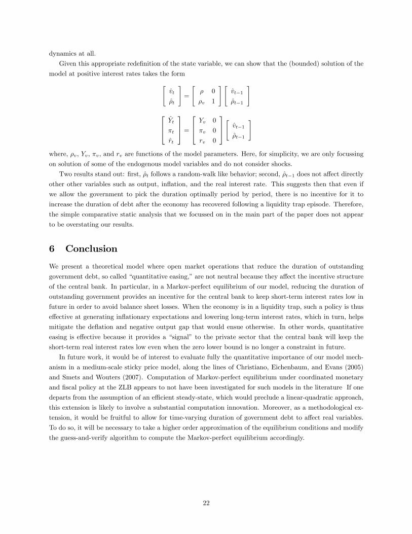
dynamics at all.
Given this appropriate redefinition of the state variable, we can show that the (bounded) solution of the
model at positive interest rates takes the form[vt
ρt
]=
[ρ 0
ρv 1
][vt−1
ρt−1
] Yt
πt
rt
=
Yv 0
πv 0
rv 0
[ vt−1
ρt−1
]
where, ρv, Yv, πv, and rv are functions of the model parameters. Here, for simplicity, we are only focussing
on solution of some of the endogenous model variables and do not consider shocks.
Two results stand out: first, ρt follows a random-walk like behavior; second, ρt−1 does not affect directly
other other variables such as output, inflation, and the real interest rate. This suggests then that even if
we allow the government to pick the duration optimally period by period, there is no incentive for it to
increase the duration of debt after the economy has recovered following a liquidity trap episode. Therefore,
the simple comparative static analysis that we focussed on in the main part of the paper does not appear
to be overstating our results.
6 Conclusion
We present a theoretical model where open market operations that reduce the duration of outstanding
government debt, so called “quantitative easing,”are not neutral because they affect the incentive structure
of the central bank. In particular, in a Markov-perfect equilibrium of our model, reducing the duration of
outstanding government provides an incentive for the central bank to keep short-term interest rates low in
future in order to avoid balance sheet losses. When the economy is in a liquidity trap, such a policy is thus
effective at generating inflationary expectations and lowering long-term interest rates, which in turn, helps
mitigate the deflation and negative output gap that would ensue otherwise. In other words, quantitative
easing is effective because it provides a “signal” to the private sector that the central bank will keep the
short-term real interest rates low even when the zero lower bound is no longer a constraint in future.
In future work, it would be of interest to evaluate fully the quantitative importance of our model mech-
anism in a medium-scale sticky price model, along the lines of Christiano, Eichenbaum, and Evans (2005)
and Smets and Wouters (2007). Computation of Markov-perfect equilibrium under coordinated monetary
and fiscal policy at the ZLB appears to not have been investigated for such models in the literature If one
departs from the assumption of an effi cient steady-state, which would preclude a linear-quadratic approach,
this extension is likely to involve a substantial computation innovation. Moreover, as a methodological ex-
tension, it would be fruitful to allow for time-varying duration of government debt to affect real variables.
To do so, it will be necessary to take a higher order approximation of the equilibrium conditions and modify
the guess-and-verify algorithm to compute the Markov-perfect equilibrium accordingly.
22

References
[1] Adam, Klaus, and Roberto M. Billi (2007), “Discretionary Monetary Policy and the Zero Lower Bound
on Nominal Interest Rates,”Journal of Monetary Economics, 54, 728-752.
[2] Alvarez, Fernando, Patrick J. Kehoe, and Pablo A. Neumeyer (2004), “The Time Consistency of Optimal
Monetary and Fiscal Policies,”Econometrica, 72, 541-567.
[3] Barro, Robert J. (1979), “On the Determination of the Public Debt,” Journal of Political Economy,
87, 940-971.
[4] Bauer, Michael D., and Glenn D. Rudebusch (2013), “The Signaling Channel for Federal Reserve Bond
Purchases,”working paper.
[5] Berriel, Tiago C., Saroj Bhattarai, and Arthur Mendes (2013), “Central Bank Balance Sheet, Liquidity
Trap, and Quantitative Easing,”working paper.
[6] Calvo, Guillermo A., and Pablo E. Guidotti (1990), “Credibility and Nominal Debt: Exploring the Role
of Maturity in Managing Inflation,”IMF Staff Papers, 37, 612-635.
[7] Calvo, Guillermo A., and Pablo E. Guidotti (1992), “Optimal Maturity of Nominal Government Debt:
An Infinite-Horizon Model,”International Economic Review, 37, 612-635.
[8] Chadha, Jagjit S., Philip Turner, and Fabrizio Zampoli (2013), “The Interest Rate Effects of Govern-
ment Debt Maturity,”working paper.
[9] Chen, Han, Vasco Curdia, and Andrea Ferrero (2012), “The Macroeconomic Effects of Large-scale Asset
Purchase Programmes,”Economic Journal, 122, 289-315.
[10] Christiano, Lawrence J., Martin Eichenbaum, and Charles Evans (2005), “Nominal Rigidities and the
Dynamic Effects of a Shock to Monetary Policy,”Journal of Political Economy, 113, 1-45.
[11] Eggertsson, Gauti B. (2006), “The Deflation Bias and Committing to Being Irresponsible,”Journal of
Money, Credit, and Banking, 38, 283-321.
[12] Eggertsson, Gauti B., and Paul Krugman (2012), “Debt, Deleveraging, and the Liquidity Trap: A
Fisher-Minsky-Koo Approach,”Quarterly Journal of Economics, 127, 1469-1513.
[13] Eggertsson, Gauti B., and Michael Woodford (2003), “The Zero Bound on Interest Rates and Optimal
Monetary Policy,”Brookings Papers on Economic Activity, 34, 139-235.
[14] Gagnon, Joseph, Matthew Raskin, Julie Ramache, and Brian Sack (2011), “The Financial Market
Effects of the Federal Reserve’s Large-Scale Asset Purchases,”International Journal of Central Banking,
7, 3-43.
[15] Hamilton, James D., and Cynthia Wu (2012), “The Effectiveness of Alternative Monetary Policy Tools
in a Zero Lower Bound Environment,”Journal of Money, Credit, and Banking, 44, 3-46.
[16] Jeanne, Olivier, and Lars E. O. Svensson (2007), “Credible Commitment to Optimal Escape from a
Liquidity Trap: The Role of the Balance Sheet of an Independent Central Bank,”American Economic
Review, 97, 474-490.
23

[17] Krishnamurthy, Arvind, and Annette Vissing-Jorgensen (2011), “The Effects of Quantitative Easing
on Interest Rates: Channels and Implications for Policy,”Brookings Papers on Economic Activity, 43,
215-287.
[18] Krugman, Paul (1998), “It’s Baaack: Japan’s Slump and the Return of the Liquidity Trap,”Brookings
Papers on Economic Activity, 29, 137-206.
[19] Lucas, Robert, and Nancy Stokey (1983), “Optimal Fiscal and Monetary Policy in an Economy without
Capital,”Journal of Monetary Economics, 12, 55-93.
[20] Faraglia, Elisa, Albert Marcet, Rigas Oikonomou, and Andrew Scott (2012), “The Impact of Govern-
ment Debt Maturity on Inflation,”working paper.
[21] Maskin, Eric, and Jean Tirole (2001), “Markov Perfect Equilibrium I: Observable Actions,”Journal of
Economic Theory, 100, 191-219.
[22] Mussa, Michael (1981), “The Role of Offi cial Intervention,”Group of Thirty Occasional Paper.
[23] Persson, Mats, Torsten Persson, and Lars E. O. Svensson (1987), “Time Consistency of Fiscal and
Monetary Policy,”Econometrica, 55, 1419-1431.
[24] Persson, Mats, Torsten Persson, and Lars E. O. Svensson (2006), “Time Consistency of Fiscal and
Monetary Policy: A Solution,”Econometrica, 74, 193-212.
[25] Rotemberg, Julio (1982), “Sticky Prices in the United States,”Journal of Political Economy, 90, 1187-
1211.
[26] Sims, Christopher A. (2011), “Stepping on a Rake: The Role of Fiscal Policy in the Inflation of the
1970s,”European Economic Review, 55, 48-56.
[27] Sims, Christopher A. (2013), “Paper Money,”American Economic Review, 103, 563-584.
[28] Smets, Frank, and Raf Wouters (2007), “Shocks and Frictions in US Business Cycles: A Bayesian DSGE
Approach,”American Economic Review, 97, 586-606.
[29] Swanson, Eric T, and John C. Williams (2013), “Measuring the Effect of the Zero Lower Bound on
Medium-and Longer-Term Interest Rates,”working paper.
[30] Wallace, Neil (1981), “A Modigliani-Miller Theorem for Open-Market Operations,”American Economic
Review, 71, 267-274.
[31] Werning, Ivan (2012), “Managing a Liquidity Trap: Monetary and Fiscal Policy,”working paper.
[32] Woodford, Michael (2001), “Fiscal Requirements for Price Stability,” Journal of Money, Credit, and
Banking, 33, 669-728.
[33] Woodford, Michael (2003), Interest and Prices. Princeton, NJ: Princeton University Press.
[34] Woodford, Michael (2012), “Methods of Policy Accommodation at the Interest-Rate Lower Bound,”in
The Changing Policy Landscape, Federal Reserve Bank of Kansas City.
24
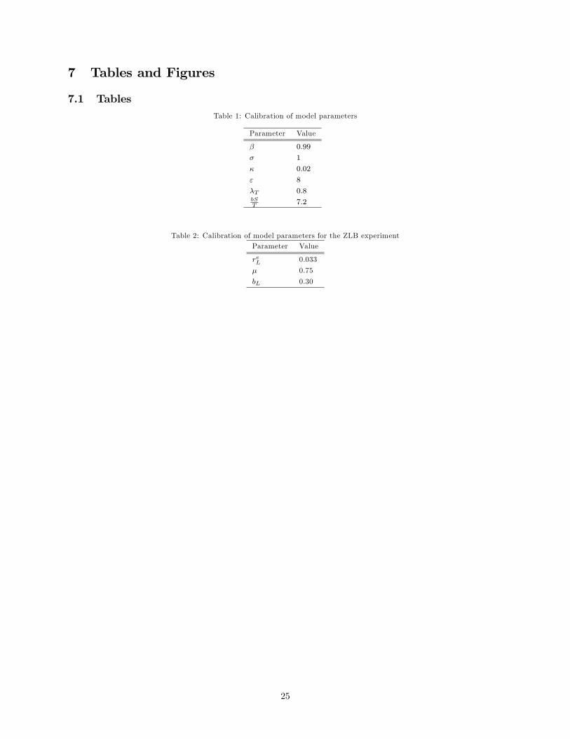
7 Tables and Figures
7.1 TablesTable 1: Calibration of model parameters
Parameter Value
β 0.99
σ 1
κ 0.02
ε 8
λT 0.8bST
7.2
Table 2: Calibration of model parameters for the ZLB experimentParameter Value
reL 0.033
µ 0.75
bL 0.30
25
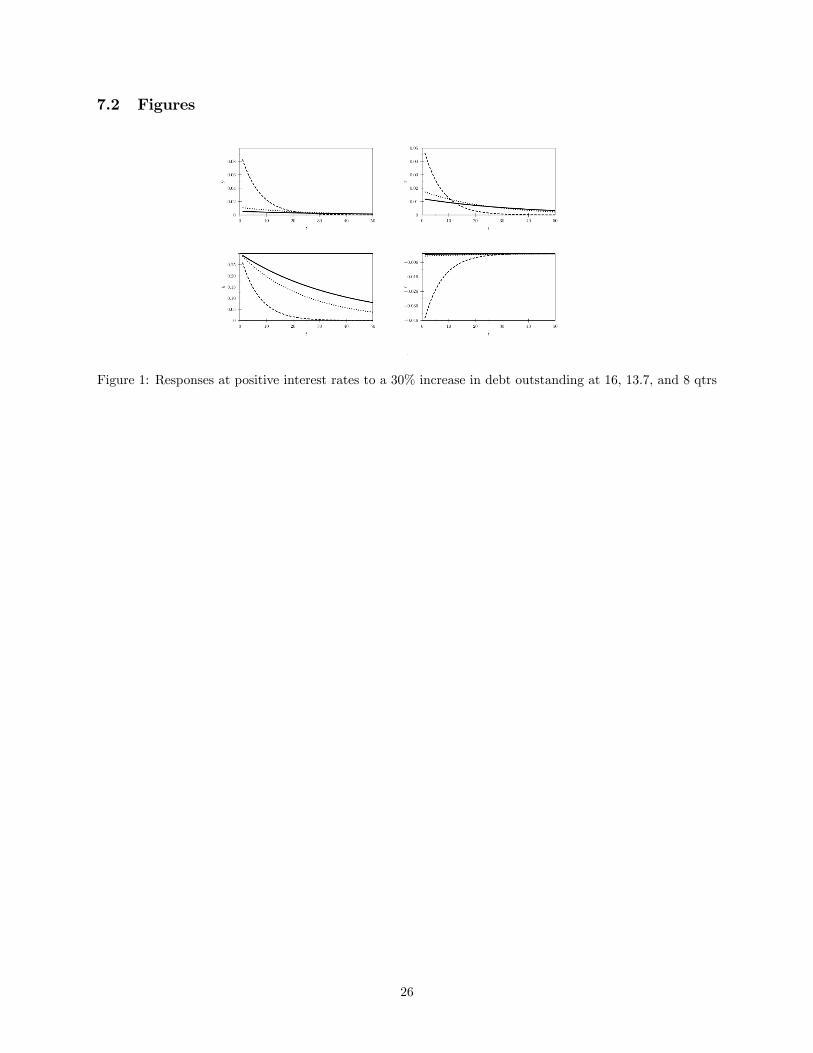
7.2 Figures
Figure 1: Responses at positive interest rates to a 30% increase in debt outstanding at 16, 13.7, and 8 qtrs
26
5 10 15 20 25Duration
0.2
0.4
0.6
0.8
1.0b
Figure 2: The effect on πb of changing the duration (quarters) of outstanding nominal government debtunder fully flexible prices.
5 10 15 20 25Duration
1.0
0.8
0.6
0.4
0.2
ib
Figure 3: The effect on ib of changing the duration (quarters) of outstanding nominal government debtunder fully rigid prices.
27

Figure 4: The effect on rb of changing the duration (quarters) of outstanding nominal government debt atdifferent levels of the slope of the Phillips curve.
Figure 5: The effect on rb of changing the duration (quarters) of outstanding nominal government debt atdifferent levels of the elasticity of substitution among varieties.
Figure 6: The effect on rb of changing the duration (quarters) of outstanding nominal government debt atdifferent levels of the weight on taxes in the loss function.
28

Figure 7: The effect on πb of changing the duration (quarters) of outstanding nominal government debt atdifferent levels of the slope of the Phillips curve.
Figure 8: The effect on πb of changing the duration (quarters) of outstanding nominal government debt atdifferent levels of the elasticity of substitution among varieties.
Figure 9: The effect on πb of changing the duration (quarters) of outstanding nominal government debt atdifferent levels of the weight on taxes in the loss function.
29
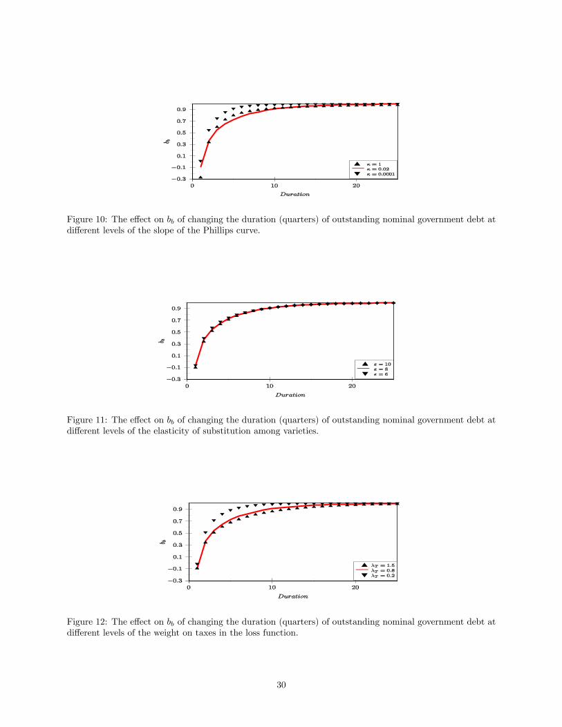
Figure 10: The effect on bb of changing the duration (quarters) of outstanding nominal government debt atdifferent levels of the slope of the Phillips curve.
Figure 11: The effect on bb of changing the duration (quarters) of outstanding nominal government debt atdifferent levels of the elasticity of substitution among varieties.
Figure 12: The effect on bb of changing the duration (quarters) of outstanding nominal government debt atdifferent levels of the weight on taxes in the loss function.
30
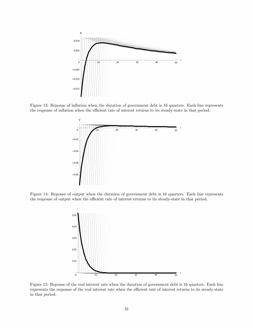
0 10 20 30 40 50t
0.015
0.010
0.005
0.005
0.010
Figure 13: Reponse of inflation when the duration of government debt is 16 quarters. Each line representsthe response of inflation when the effi cient rate of interest returns to its steady-state in that period.
0 10 20 30 40 50t
0.08
0.06
0.04
0.02
Y
Figure 14: Reponse of output when the duration of government debt is 16 quarters. Each line representsthe response of output when the effi cient rate of interest returns to its steady-state in that period.
0 10 20 30 40 50t
0.01
0.02
0.03
0.04
0.05
r
Figure 15: Reponse of the real interest rate when the duration of government debt is 16 quarters. Each linerepresents the response of the real interest rate when the effi cient rate of interest returns to its steady-statein that period.
31
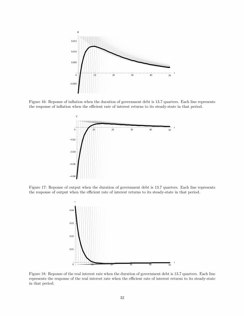
0 10 20 30 40 50t
0.005
0.005
0.010
0.015
Figure 16: Reponse of inflation when the duration of government debt is 13.7 quarters. Each line representsthe response of inflation when the effi cient rate of interest returns to its steady-state in that period.
0 10 20 30 40 50t
0.08
0.06
0.04
0.02
Y
Figure 17: Reponse of output when the duration of government debt is 13.7 quarters. Each line representsthe response of output when the effi cient rate of interest returns to its steady-state in that period.
0 10 20 30 40 50t
0.01
0.02
0.03
0.04
r
Figure 18: Reponse of the real interest rate when the duration of government debt is 13.7 quarters. Each linerepresents the response of the real interest rate when the effi cient rate of interest returns to its steady-statein that period.
32

0 10 20 30 40 50t
0.01
0.02
0.03
Figure 19: Reponse of inflation when the duration of government debt is 9.11 quarters. Each line representsthe response of inflation when the effi cient rate of interest returns to its steady-state in that period.
0 10 20 30 40 50t
0.01
0.02
0.03
0.04
0.05
Y
Figure 20: Reponse of output when the duration of government debt is 9.11 quarters. Each line representsthe response of inflation when the effi cient rate of interest returns to its steady-state in that period.
33

0 10 20 30 40 50t
0.020
0.015
0.010
0.005
r
Figure 21: Reponse of the real interest rate when the duration of government debt is 9.11 quarters. Each linerepresents the response of the real interest rate when the effi cient rate of interest returns to its steady-statein that period.
0 10 20 30 40 50t
0.04
0.03
0.02
0.01
0.01
i
Figure 22: Reponse of the short-term nominal interest rate when the duration of government debt is 16quarters. Each line represents the response of the short-term interest rate when the effi cient rate of interestreturns to its steady-state in that period.
0 10 20 30 40 50t
0.05
0.10
S
Figure 23: Reponse of the long-term nominal interest rate when the duration of government debt is 16quarters. Each line represents the response of the long-term interest rate when the effi cient rate of interestreturns to its steady-state in that period.
34

0 10 20 30 40 50t
0.04
0.03
0.02
0.01
0.01
i
Figure 24: Reponse of the short-term nominal interest rate when the duration of government debt is 13.7quarters. Each line represents the response of the short-term interest rate when the effi cient rate of interestreturns to its steady-state in that period.
0 10 20 30 40 50t
0.05
0.10
S
Figure 25: Reponse of the long-term nominal interest rate when the duration of government debt is 13.7quarters. Each line represents the response of the long-term interest rate when the effi cient rate of interestreturns to its steady-state in that period.
35

0 10 20 30 40 50t
0.002
0.004
0.006
0.008
T
Figure 26: Increase in taxes a result of reneging on optimal policy when the duration of government debtis 16 quarters. Each line represents the response of the long-term interest rate when the effi cient rate ofinterest returns to its steady-state in that period.
0 10 20 30 40 50t
0.005
0.010
0.015
T
Figure 27: Increase in taxes a result of reneging on optimal policy when the duration of government debtis 13.7 quarters. Each line represents the response of the long-term interest rate when the effi cient rate ofinterest returns to its steady-state in that period.
Figure 28: Effects of quantitative easing on output at different values of λT .
36
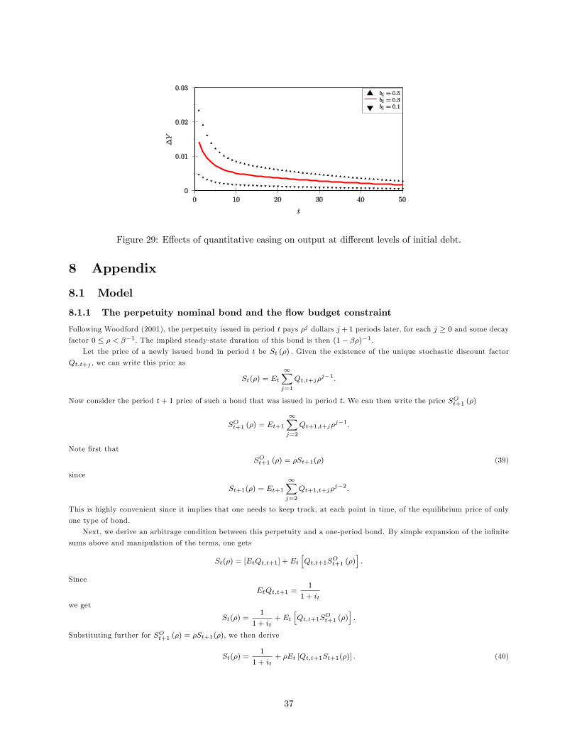
Figure 29: Effects of quantitative easing on output at different levels of initial debt.
8 Appendix
8.1 Model
8.1.1 The perpetuity nominal bond and the flow budget constraint
Following Woodford (2001), the perpetuity issued in period t pays ρj dollars j+ 1 periods later, for each j ≥ 0 and some decay
factor 0 ≤ ρ < β−1. The implied steady-state duration of this bond is then (1− βρ)−1.
Let the price of a newly issued bond in period t be St (ρ) . Given the existence of the unique stochastic discount factor
Qt,t+j , we can write this price as
St(ρ) = Et
∞∑j=1
Qt,t+jρj−1.
Now consider the period t+ 1 price of such a bond that was issued in period t. We can then write the price SOt+1 (ρ)
SOt+1 (ρ) = Et+1
∞∑j=2
Qt+1,t+jρj−1.
Note first that
SOt+1 (ρ) = ρSt+1(ρ) (39)
since
St+1(ρ) = Et+1
∞∑j=2
Qt+1,t+jρj−2.
This is highly convenient since it implies that one needs to keep track, at each point in time, of the equilibrium price of only
one type of bond.
Next, we derive an arbitrage condition between this perpetuity and a one-period bond. By simple expansion of the infinite
sums above and manipulation of the terms, one gets
St(ρ) = [EtQt,t+1] + Et[Qt,t+1S
Ot+1 (ρ)
].
Since
EtQt,t+1 =1
1 + itwe get
St(ρ) =1
1 + it+ Et
[Qt,t+1S
Ot+1 (ρ)
].
Substituting further for SOt+1 (ρ) = ρSt+1(ρ), we then derive
St(ρ) =1
1 + it+ ρEt [Qt,t+1St+1(ρ)] . (40)
37

Finally, consider the flow budget constraint of the government
BSt + St(ρ)Bt = (1 + it−1)BSt−1 +(ρ0 + SOt (ρ)
)Bt−1 + Pt (Ft − Tt) .
This can be simplified using SOt+1 (ρ) = ρSt+1(ρ) to
BSt + St(ρ)Bt = (1 + it−1)BSt−1 + (1 + ρSt(ρ))Bt−1 + Pt (Ft − Tt) .
This is the form in which we write down the flow budget constraint of the household and the government in the main text.
8.1.2 Functional forms
We make the following functional form assumptions on preferences and technology
u (C, ξ) = ξC1σC1−
1σ
1− 1σ
v (h(i), ξ) = ξλh(i)1+φ
1 + φ
g (G, ξ) = ξG1σG1−
1σ
1− 1σ
y(i) = h(i)κ
d(Π) = d1 (Π− 1)2
S(T)
= s1 (T − T )2
where we only consider a discount factor shock ξ. Note that ξ = 1 in steady-state and that in steady state, we scale hours such
that Y = 1 as well. This implies that we can derive
v (Y, ξ) =1
1 + φλξY
1+φκ .
8.2 Effi cient equilibriumAs benchmark, we first derive the effi cient allocation.
Using Gt = Ft − s(Tt − T ) = F − s(Tt − T ), the social planner’s problem can be written as
maxu (Ct, ξt) + g (F − s(Tt − T ))− v (Yt)
st
Yt = Ct + F.
Formulate the Lagrangian
Lt = u (Ct, ξt) + g (F − s(Tt − T ))− v (Yt)
+ φ1t (Yt − Ct − F )
FOCs (where all the derivatives are to be equated to zero)
∂Lt
∂Yt= −vY + φ1t
∂Lt
∂Ct= uC + φ1t [−1]
∂Lt
∂Tt= gG
(−s′(Tt − T )
)Eliminating the Lagrange multiplier gives
uC = vY
gG(−s′(Tt − T )
)= 0.
Note that we make the following functional form assumptions on the tax collection cost
s(0) = 0; s′(0) = 0.
38
Thus, when taxes are at steady state, that is, Tt = T, then s(Tt−T ) = s′(Tt−T ) = 0. But note that we will allow for s′′
(0) > 0.
Effi cient allocation thus requires
uC = vY
Tt = T.
In steady state, without aggregate shocks, we have
Y = C + F
uC = vY
Tt = T.
8.3 Non-linear markov equilibrium
8.3.1 Optimal policy under discretion
The policy problem can be written as
J (bt−1, ξt) = max [U (Λt, ξt) + βEtJ (bt, ξt+1)]
st
St(ρ)bt = (1 + ρSt(ρ)) bt−1Π−1t + (F − Tt) .
1 + it =uC (Ct, ξt)
βfet
it ≥ 0
St(ρ) =1
uC (Ct, ξt)βget
εYt
[ε− 1
ε(1 + s)uC (Ct, ξt)− vy (Yt, ξt)
]+ uC (Ct, ξt) d
′ (Πt) Πt = βhet
Yt = Ct + F + d (Πt)
fet = Et[uC (Ct+1, ξt+1) Π−1t+1
]= fe (bt, ξt)
get = Et[uC (Ct+1, ξt+1) Π−1t+1 (1 + ρSt+1(ρ))
]= ge (bt, ξt)
het = Et[uC (Ct+1, ξt+1) d′ (Πt+1) Πt+1
]= he (bt, ξt)
Formulate the period Lagrangian
Lt = u (Ct, ξt) + g (F − s(Tt − T ))− v (Yt) + βEtJ (bt, ξt+1)
+ φ1t(St(ρ)bt − (1 + ρSt(ρ)) bt−1Π−1t − (F − Tt)
)+ φ2t
(βfet −
uC (Ct, ξt)
1 + it
)+ φ3t (βget − uC (Ct, ξt)St(ρ))
+ φ4t
(βhet − εYt
[ε− 1
ε(1 + s)uC (Ct, ξt)− vy (Yt, ξt)
]− uC (Ct, ξt) d
′ (Πt) Πt
)+ φ5t (Yt − Ct − F − d (Πt))
+ ψ1t(fet − fe (bt, ξt)
)+ ψ2t (get − ge (bt, ξt))
+ ψ3t(het − he (bt, ξt)
)+ γ1t (it − 0)
39
First-order conditions (where all the derivatives should be equated to zero)
∂Ls
∂Πt= φ1t
[(1 + ρSt(ρ)) bt−1Π−2t
]+ φ4t
[−uCd
′′Πt − uCd
′]+ φ5t
[−d′
]∂Ls
∂Yt= −vY + φ4t
[−ε(ε− 1
ε(1 + s)uC
)+ εYtvyy + εvy
]+ φ5t
∂Ls
∂it= φ2t
[uC (1 + it)
−2]
+ γ1t
∂Ls
∂St= φ1t
[bt − ρbt−1Π−1t
]+ φ3t [−uC ]
∂Ls
∂Ct= uC + φ2t
[−uCC (1 + it)
−1]
+ φ3t [−uCCSt(ρ)] + φ4t
[−εYt
ε− 1
ε(1 + s)uCC − uCCd′Πt
]+ φ5t [−1]
∂Ls
∂Tt= gG
(−s′(Tt − T )
)+ φ1t
∂Ls
∂bt= βEtJb (bt, ξt+1) + φ1t [St(ρ)] + ψ1t
[−feb
]+ ψ2t [−geb ] + ψ3t
[−heb
]∂Ls
∂fet= βφ2t + ψ1t
∂Ls
∂get= βφ3t + ψ2t
∂Ls
∂het= βφ4t + ψ3t
The complementary slackness conditions are
γ1t ≥ 0, it ≥ 0, γ1tit = 0
While the envelope condition is
Jb (bt−1, ξt) = φ1t[− (1 + ρSt(ρ)) Π−1t
]This also implies that
βEtJb (bt, ξt+1) = βEtφ1t+1[− (1 + ρSt+1(ρ)) Π−1t+1
]8.3.2 Steady-state
A Markov-perfect steady-state is non-trivial to characterize because generally, we need to take derivatives of an unknown
function, as is clear from the FOCs. Here, we will rely on the fact that given an appropriate production subsidy, the Markov-
perfect steady-state will be the same as the effi cient steady-state derived above.
First, note that this requires no resource loss from price-adjustment costs, which in turn requires
d (Π) = 0
and thereby ensures
Y = C + F
This means that we need
Π = 1.
Also, this implies
d′ (Π) = 0.
Next, note from the Phillips curve that this means, we need
ε− 1
ε(1 + s)uC − vy = 0.
Now, since the effi cient steady-state has uC = vY , the production subsidy then has to satisfy
ε− 1
ε(1 + s) = 1.
40

We will be looking at a steady-state with positive interest rates
1 + i =1
β
which means that
γ1 = 0
and that from the FOC wrt it we have
φ2 = 0.
Also, given that taxes are at steady-state, gG (−s′(Tt − T )) = 0, from the FOC wrt Tt
φ1 = 0.
Given this, in turn, we have from the FOC wrt Stφ3 = 0.
Then, given that d′ = 0 in steady-state and d′′ is not, and since φ1 = 0, it gives from the FOC wrt to Πt
φ4 = 0.
Note that this is highly convenient since these Lagrange multipliers being zero implies
ψ1 = ψ2 = ψ3 = 0.
Thus, we do not need to worry about the derivatives of the unknown functions.
This proposed steady-state is consistent with other FOCs. For example, the FOC wrt Yt is now given by
φ5 = vY
and that the FOC wrt Ct is given by
uC = φ5
which implies
vY = uC .
Finally, FOC wrt bt implies
βJb = βφ1[− (1 + ρS(ρ)) Π−1
]= 0
which is also consistent with the conjectured guess.
Finally, the guess of the steady-state is also consistent with the other model equilibrium conditions, with S(ρ) given by
S(ρ) = β [(1 + ρS(ρ))]
that is
S(ρ) =β
1− ρβ.
Then b and F are linked by
S(ρ)b = (1 + ρS(ρ)) b+ (F − T )
that is
T = F +1− β1− ρβ
b.
8.3.3 First-order approximation
We now take a log-linear approximation of the Markov perfect FOCs and the private sector equilibrium conditions around
the steady-state above. Also, lets normalize the scale of the economy (with appropriate scaling of hours) so that Y = 1. This
implies C = 1− F. Also the shock ξt takes a value of 1 in steady-state.
Private sector equilibrium conditions We first start with the private sector equilibrium conditions. We denote
variables that are in log-deviations from their respective steady-states by hats, except for ıt.We denote variables in steady-state
by bars.
First,
Yt = Ct + F + d (Πt)
41
gives
Yt = CCt
Second,
εYt
[ε− 1
ε(1 + s)uC (Ct, ξt)− vy (Yt, ξt)
]+ uC (Ct, ξt) d
′ (Πt) Πt = βEt[uC (Ct+1, ξt+1) d′ (Πt+1) Πt+1
]gives
uCd′′πt + εuCC CCt − εvyyYt−εvyξ ξt + εuCξ ξt = βuCd
′′Etπt+1
which can be simplified by making use of the log-linearized resource constraint above to yield
uCd′′πt + ε (uCC − vyy) Yt = βuCd
′′Etπt+1
πt = βEtπt+1 +ε (vyy − uCC)
uCd′′Yt.
Third,
1 + it =uC (Ct, ξt)
βEt[uC (Ct+1, ξt+1) Π−1t+1
]gives
uCC CCt + uCξ ξt = uC ıt + uCCEtCCt+1 + uCξEtξt+1 − uCEtπt+1
which can be simplified by making use of the log-linearized resource constraint above to yield
uCC Yt + uCξ ξt = uC ıt + uCCEtYt+1 + uCξEtξt+1 − uCEtπt+1
and
Yt = EtYt+1 +uC
uCC[ıt − Etπt+1] +
uCξ
uCC
[Etξt+1 − ξt
]Note here that this implies that the effi cient rate of interest is given by
ret = −uCξ
uC
[Etξt+1 − ξt
].
Fourth,
St(ρ) =1
uC (Ct, ξt)βEt
[uC (Ct+1, ξt+1) Π−1t+1 (1 + ρSt+1(ρ))
]gives
SuCC CCt + SuCξ ξt + uC SSt = β(1 + ρS
)uCCEtCCt+1 + β
(1 + ρS
)uCξEtξt+1 − β
(1 + ρS
)uCEtπt+1 + βρSuCEtSt+1
which can be simplifies by making use of the log-linearized resource constraint above to yield
SuCC Yt + SuCξ ξt + uC SSt = β(1 + ρS
)uCCEtYt+1 + β
(1 + ρS
)uCξEtξt+1 − β
(1 + ρS
)uCEtπt+1 + βρSuCEtSt+1.
Note here that by using the log-linearized Euler equation above, one can further simplify as
S[uC ıt + uCCEtYt+1 + uCξEtξt+1 − uCEtπt+1
]+ uC SSt
= β(1 + ρS
)uCCEtYt+1 + β
(1 + ρS
)uCξEtξt+1 − β
(1 + ρS
)uCEtπt+1 + βρSuCEtSt+1
or [uC ıt + uCCEtYt+1 + uCξEtξt+1 − uCEtπt+1
]+ uC St
=β(1 + ρS
)S
uCCEtYt+1 +β(1 + ρS
)S
uCξEtξt+1 −β(1 + ρS
)S
uCEtπt+1 + βρuCEtSt+1.
Moreover, sinceβ(1 + ρS
)S
= 1
we have finally as the asset-pricing condition
ıt + St = βρEtSt+1.
Fifth,
St(ρ)bt = (1 + ρSt(ρ)) bt−1Π−1t + (F − Tt)
42

gives
bt + St = ρSt +
(1 + ρS
)S
bt −(1 + ρS
)S
πt −T
SbTt
which is simplified further as
bt = β−1bt − β−1πt − (1− ρ) St −T
SbTt.
Then, finally, the expectation functions are given by
fet = Et[uC (Ct+1, ξt+1) Π−1t+1
]= uCCEtYt+1 + uCξEtξt+1 − uC πt+1
get = Et[uC (Ct+1, ξt+1) Π−1t+1 (1 + ρSt+1(ρ))
]=(1 + ρS
)uCCEtYt+1+
(1 + ρS
)uCξEtξt+1−
(1 + ρS
)uCEtπt+1+ρSuCEtSt+1
het = Et[uC (Ct+1, ξt+1) d′ (Πt+1) Πt+1
]= uCd
′′Etπt+1
Markov-perfect FOCs Here, note that since all the Lagrange multipliers except one are zero in steady-state, what we
mean by hats will in fact only be deviations from steady-state for all the lagrange multipliers (as opposed to log-deviations).
First,
φ1t[(1 + ρSt(ρ)) bt−1Π−2t
]+ φ4t
[−uCd
′′Πt − uCd
′]+ φ5t
[−d′
]= 0
gives (1 + ρS
)bφ1t − uCd
′′φ4t − φ5d′′πt = 0
and since φ5 = vy = uC (1 + ρS
)bφ1t − uCd
′′φ4t − uCd′′πt = 0.
Second,
−vY + φ4t
[−ε(ε− 1
ε(1 + s)uC
)+ εYtvyy + εvy
]+ φ5t = 0
gives
−vY Y Y Yt +[εY vyy
]φ4t + φ5t = 0.
Third,
φ2t[uC (1 + it)
−2]
+ γ1t = 0
gives
uCβ2φ2t + γ1t = 0.
Fourth,
φ1t[bt − ρbt−1Π−1t
]+ φ3t [−uC ] = 0
gives [(1− ρ) b
]φ1t − uC φ3t = 0.
Fifth,
uC + φ2t[−uCC (1 + it)
−1]
+ φ3t [−uCCSt(ρ)] + φ4t
[−εYt
ε− 1
ε(1 + s)uCC − uCCd′Πt
]+ φ5t [−1] = 0
gives
Yt +uCξ
uCCξt − βφ2t − Sφ3t − εφ4t −
1
uCCφ5t = 0.
Sixth,
gG(−s′(Tt − T )
)+ φ1t = 0
gives
−gGs′′T Tt + φ1t = 0.
Seventh (after some replacements),
βEtφ1t+1[− (1 + ρSt+1(ρ)) Π−1t+1
]+ φ1t [St(ρ)] + βφ2t
[feb]
+ βφ3t [geb ] + βφ4t[heb]
= 0
gives
−SEtφ1t+1 + Sφ1t + βfbφ2t + βgbφ3t + βhbφ4t = 0.
43

8.4 Linear-quadratic approach
8.4.1 Linear approximation of equilibrium conditions
We approximate around an effi cient non-stochastic steady-state where Π = 1. For simplicity, from here on we will assume that
the only shock that hits the economy is a discount factor shock given by ψ. Standard manipulations that are prevalent in the
literature, for example in Woodford (2003), and as shown above in the Markov perfect equilibrium, give (24) and (25) where
σ = σCYand k = ε
(σ−1+φ)d′′ . Here we again detail the derivations of (26) and (27). Given
St(ρ) =1
uC (Ct, ξt)βEt
[uC (Ct+1, ξt+1) Π−1t+1 (1 + ρSt+1(ρ))
],
and
1 + it =uC (Ct, ξt)
βEt[uC (Ct+1, ξt+1) Π−1t+1
]and the functional form assumptions above together with in steady state 1 + i = β−1, log-linearization gives immediately
St = −ıt + ρβEtSt+1.
Next, given
St(ρ)bt = (1 + ρSt(ρ)) bt−1Π−1t + (Ft − Tt)
and that we assume Ft = F and have from steady state S = β1−ρβ , T = F + 1−β
1−ρβ b, log-linearization gives immediately
bt = β−1bt−1 − β−1πt − (1− ρ)St − ψTt.
Note that also the following relationship holds in steady state F = G. We finally derive an expression for ret , the effi cient rate
of interest
ret = σ−1 (ψt − Etψt+1) .
8.4.2 Quadratic approximation of household utility
For household utility, we need to approximate the following three components
u (Yt − F − d(Πt), ξt) ; g (F − S(Tt − T ), ξt) ; v (Yt, ξt) .
Standard manipulations that are prevalent in the literature, for example in Woodford (2003), give as a second-order approxi-
mation to household utility
1
2
−σ(T 2t(F − Y
)s′′(T)
+ Fd′′(1)Π2t
)+ 2σYt
(−Y + F ξt + F
)+ Y 2t
σ(F − Y
) +
1
2Y
(d′′(1)Π2
t
F − Y+ ξt
(2σ
σ − 1− 2Yt
F − Y
)+
2σ
σ − 1
)− 1
22λ(ξt + 1
)YtY
φ − 1
2
2λ(ξt + 1
)Y φ+1
φ+ 1− 1
2λφY 2t Y
φ−1 + tip
which is in turn given as
1
2
(Y 2t
(1
Fσ − σY− λφY φ−1
)+ T 2t
(−s′′
(T))− 2
(ξt + 1
)Yt(λY φ − 1
)− d′′(1)Π2
t
)+ tip.
Now lets multiply everything by 1φ+σ−1
and consider effi cient equilibrium in steady-state (uC = vY ), together with the scaling
that λY φ = 1 and Y = C + F = 1, to get
−σT 2t s
′′ (T )2 (φσ + 1)
− σd′′(1)Π2t
2 (φσ + 1)− Y 2t
2
So, finally, we get as approximation
−[λππ
2t + Y 2t + λT T
2t
]where
λT =s′′(T)
φ+ σ−1
44
λπ =d′′(1)
(φ+ σ−1)=ε
κ.
8.4.3 Markov-perfect equilibrium at positive interest rates
Given the Lagrangian where the expectation functions are substituted and the shocks are suppressed
Lt =1
2(λππ
2t + Y 2t + λT T
2t ) + βEtV (bt, r
et+1) + φ1t[Yt − Ybbt + σıt − σπbbt − σret ]
+ φ2t[πt − κYt − βπbbt] + φ3t[bt − β−1bt−1 + β−1πt + (1− ρ)St + ψTt] + φ4t[St + ıt − ρβSbbt]
the first-order necessary conditions are given by
∂L
∂πt= λππt + φ2t + β−1φ3t = 0
∂L
∂Yt= Yt + φ1t − κφ2t = 0
∂L
∂Tt= λTTt + ψφ3t = 0
∂L
∂it= σφ1t + φ4t = 0
∂L
∂St= φ3t(1− ρ) + φ4t = 0
∂L
∂bt= βEtVb(bt, r
et+1)− (Yb + σπb)φ1t − βπbφ2t + φ3t − ρβSbφ4t = 0
while the envelope condition is given by
Vb(bt−1, ret ) = −β−1φ3t
which implies
EtVb(bt, ret+1) = −β−1Etφ3t+1.
We can then combine the envelope condition with the last FOC to yield
−Etφ3t+1 − (Yb + σπb)φ1t − βπbφ2t + φ3t − ρβSbφ4t = 0.
To summarize, we have
λππt + φ2t + β−1φ3t = 0
Yt + φ1t − κφ2t = 0
λTTt + ψφ3t = 0
σφ1t + φ4.t = 0
φ3t(1− ρ) + φ4t = 0
−Etφ3t+1 − (Yb + σπb)φ1t − βπbφ2t + φ3t − ρβSbφ4t = 0
Yt = EtYt+1 − σ(ıt − Etπt+1 − ret )
πt = κYt + βEtπt+1
bt = β−1bt−1 − β−1πt − (1− ρ)St − ψTt
St = −ıt + ρβEtSt+1
which can be simplified to get
λππt + κ−1Yt = [κ−1 (1− ρ)σ−1 + β−1]bS
TλT Tt
[1− βπbκ−1 (1− ρ)σ−1 − (Yb + σπb) (1− ρ)σ−1 + ρβSb(1− ρ)]Tt = − (ψ)λ−1T βπbκ−1Yt + EtTt+1
Yt = EtYt+1 − σ(ıt − Etπt+1 − ret )
πt = κYt + βEtπt+1
bt = β−1bt−1 − β−1πt − (1− ρ)St − ψTt
St = −ıt + ρβEtSt+1.
45

The final step is then to match coeffi cients after replacing the conjectured solutions
λππbbt−1 + κ−1 (Ybbt−1) = [κ−1(1− ρ)σ−1 + β−1]bS
TλT (Tbbt−1)
[1− βπbκ−1 (1− ρ)σ−1 − (Yb + σπb) (1− ρ)σ−1 + ρβSb(1− ρ)] [Tbbt−1] = − (ψ)λ−1T βπbκ−1 [Ybbt−1] + [Tb (bbbt−1)]
Ybbt−1 = Yb [bbbt−1]− σ((ibbt−1)− [πb [bbbt−1]])
πbbt−1 = κ [Ybbt−1] + βπb [bbbt−1]
bbbt−1 = β−1bt−1 − β−1 [πbbt−1]− (1− ρ) [Sbbt−1]− ψ [Tbbt−1]
Sbbt−1 = − (ibbt−1) + ρβSb [bbbt−1]
which in turn can be simplified to get
λππb + κ−1Yb = [κ−1(1− ρ)σ−1 + β−1]bS
TλTTb (41)
[(1− ρ)−1 − βπbκ−1σ−1 − (Yb + σπb)σ−1 + ρβSb] (1− ρ)Tb = − (ψ)λ−1T βπbκ
−1Yb + Tbbb (42)
Yb = Ybbb − σ(ib − πbbb) (43)
πb = κYb + βπbbb (44)
bb = β−1 − β−1πb − (1− ρ)Sb − ψTb (45)
Sb = −ib + ρβSbbb. (46)
We now show some properties of πb analytically. First, note that we will be restricting to stationary solutions, that is one
where | bb |< 1. Manipulations of (41)-(46) above lead to the following closed-form expression for πb
πb =(1− βbb)
β[TlVχ [λπ + κ−1κ−1 (1− βbb)] + [(1− ρ)σ−1κ−1 (1− bb) + β−1] (1− βbb) (1− ρβbb)−1
]where χ =
[[κ−1σ−1(1− ρ) + β−1]
bS
TλT
]−1.
Since | bb |< 1, it is clear that πb > 0 for all ρ < 1, . What happens whenρ > 1? Numerically, we have found that often πb > 0
still, but sometimes in fact it can hit zero (and then actually go negative if ρ is increased further). It is in fact possible to
pin-down analytically when πb = 0. Note that from (44), if πb = 0, then Yb = 0. This then implies that for this to be supported
as a solution for all possible values of Tb, from (41), it must be the case that
[κ−1(1− ρ)σ−1 + β−1] = 0
which in turn implies that
ρ = 1 + β−1σκ.
In this knife-edge case, note that one needs ρ > 1. Moreover, since the upper bound on ρ is β−1, one needs to ensure that
1 + β−1σκ < β−1 or σκ < 1− β.
This is a fairly restrictive parameterization (not fulfilled in our baseline, for example). Still, it is instructive to note that in
this case of when πb does reach 0, then it is indeed possible to show analytically that πb declines as duration is increased while
comparing ρ = 0 with ρ = 1 + β−1σκ or ρ = 1 with ρ = 1 + β−1σκ.
8.5 Equivalence of the two approachesWe now show the equivalence of the linearized dynamic systems for non-linear and linear-quadratic approaches.
Consider the system of equations describing private sector equilibrium and optimal government policy
Yt = EtYt+1 +uC
uCC[ıt − Etπt+1 − ret ]
πt =ε (vyy − uCC)
uCd′′Yt + βEtπt+1.
ıt + St = βρEtSt+1.
46

bt = β−1bt − β−1πt − (1− ρ) St −T
SbTt.
(1 + ρS
)bφ1t − uCd
′′φ4t − φ5d′′πt = 0
−vY Y Y Yt +[εY vyy
]φ4t + φ5t = 0
uCβ2φ2t + γ1t = 0
[(1− ρ) b
]φ1t − uC φ3t = 0.
Yt +uCξ
uCCξt − βφ2t − Sφ3t − εφ4t −
1
uCCφ5t = 0.
−gGs′′T Tt + φ1t = 0.
−SEtφ1t+1 + Sφ1t + βfbφ2t + βgbφ3t + βhbφ4t = 0.
Under additional functional assumptions outlined in previous sections we get
vY Y = φY−1
= φ
uCC = −σ−1C−1 = −σ−1
uCξ = 1
uC = 1
gG = 1
φ5 = 1
Y = 1
The first four equations are equivalent to their counterparts in the LQ-approach once one use the functional form assump-
tions to getuC
uCC= −σ
and introduce new notationε (vyy − uCC)
uCd′′= κ.
The latter relation impliesε(φ+ σ−1
)κ
= d′′.
Let us guess solutions for all variables for the case when the ZLB is slack as a linear function of bt−1 and ret . Then the
expectations will take form
fet = uCCEtYt+1 + uCξEtξt+1 − uCEtπt+1 = feb bbt−1 + fer ret
get =(1 + ρS
)uCCEtYt+1 +
(1 + ρS
)uCξEtξt+1 −
(1 + ρS
)uCEtπt+1 + ρSuCEtSt+1 = geb bbt−1 + ger r
et
het = uCd′′Etπt+1 = heb bbt−1 + her r
et
where
feb = −b−1(σ−1Yb + πb
)geb = −σ−1b−1
(1 + ρS
)Yb −
(1 + ρS
)b−1πb + ρSSbb
−1
47
heb =ε(φ+ σ−1
)κ
πbb−1
Also under the assumption about the process ξt we get
Etξt+1 = µξt
and
ret = −uCξ
uC
[µξt − ξt
]= ξt(1− µ).
When the economy is out of ZLB ret = 0.
Now we can find explicit representation for the lagrange multipliers
φ1t = s′′T Tt.
φ2t = 0
φ3t = [(1− ρ)] s′′T Tt.
φ4t =κ
ε (φ+ σ−1)
(1 + ρS
)bs′′T Tt − πt
φ5t = φYt − φκ
(φ+ σ−1)
(1 + ρS
)s′′T Tt + εφπt
So the last two equations take the form
επt = −Yt +1
(φ+ σ−1)
[σ−1S (1− ρ) + κ
(1 + ρS
)]bs′′T Tt.
Ss′′T Tt +
(ρβSb − σ−1Yb − πb
)b−1 (1− ρ) Sbs
′′T Tt + b−1πbSbs
′′T Tt − β
ε(φ+ σ−1
)κ
πbb−1πt = s
′′T SEtTt+1.
which after straightforward manipulations become
ε
κπt + Ytκ
−1 =[σ−1 (1− ρ)κ−1 + β−1
] bST
T 2s′′
(φ+ σ−1)Tt.
(1 +
(ρβSb − σ−1Yb − πb
)(1− ρ) + πb
) SbT
s′′T 2
(φ+ σ−1)Tt − β
ε
κπbπt =
s′′T 2
(φ+ σ−1)
bS
TEtTt+1.
These two equations are equivalent for the last two equations from the dynamic system obtained in LQ—approach once we
use the derived weights from the quadratic approximation of the loss function
λT =s′′T 2
(φ+ σ−1)
λπ = κ−1ε.
8.6 Computation at ZLBIn our experiment the debt is kept fixed at the zero lower bound at bL . Moreover, at the zero lower bound, ıt = 1 − β−1.Given the specific assumptions on the two-state Markov shock process, the equilibrium is described by the system of equations
Yt = −σ(−πb(1− µ)bt − ret − µπL + ıt
)+ (1− µ)btYb + µYL,
πt = β(πb(1− µ)bt + µπL
)+ κYt,
ıt = 1− β−1,
bt = bL,
St = −ıt + ρβ ((1− µ)SbbL + µSL) .
48

where variables with a b subscript denote the solution we compute at positive interest rates while variables with a L subscript
denote values at the ZLB. The solution to this system is
Yt = YL =βπb(µ− 1)bL
κ−
(1− βµ)(βπb(1− µ)2bL − κ (bL (πb(µ− 1)σ + (µ− 1)Yb)− σret + σiL)
)κ(κµσ − (1− µ)(1− βµ))
,
πt = πL =− βπb(1− µ)2bL − κ (bL (πb(µ− 1)σ + (µ− 1)Yb)− σret + σiL)
κµσ − (1− µ)(1− βµ),
ıt = iL =1− β−1, bt = bL,
St = SL =ρβ(1− µ)SbbL − ıt
1− ρβµ
where the solution for variables with a b subscript has already been provided above.
8.7 Non-linear markov equilibrium of extended modelWe now consider a model where the duration of government debt is time-varying and chosen optimally by the government.
The policy problem can be written as
J (bt−1, ρt−1, ξt) = max [U (Λt, ξt) + βEtJ (bt, ρt, ξt+1)]
st
St(ρt)bt = (1 + ρt−1Wt(ρt−1)) bt−1Π−1t + (F − Tt) .
1 + it =uC (Ct, ξt)
βfet
it ≥ 0
St(ρt) =1
uC (Ct, ξt)βget
Wt(ρt−1) =1
uC (Ct, ξt)βjet
εYt
[ε− 1
ε(1 + s)uC (Ct, ξt)− vy (Yt, ξt)
]+ uC (Ct, ξt) d
′ (Πt) Πt = βhet
Yt = Ct + F + d (Πt)
fet = Et[uC (Ct+1, ξt+1) Π−1t+1
]= fe (bt, ρt, ξt)
get = Et[uC (Ct+1, ξt+1) Π−1t+1 (1 + ρtSt+1(ρt))
]= ge (bt, ρt, ξt)
het = Et[uC (Ct+1, ξt+1) d′ (Πt+1) Πt+1
]= he (bt, ρt, ξt)
jet = Et[uC (Ct+1, ξt+1) Π−1t+1 (1 + ρt−1Wt+1(ρt−1))
]= je (bt, ρt, ξt)
49

Formulate the period Lagrangian
Lt = u (Ct, ξt) + g (F − s(Tt − T ))− v (Yt) + βEtJ (bt, ρt, ξt+1)
+ φ1t(St(ρt)bt − (1 + ρt−1Wt(ρt−1)) bt−1Π−1t − (F − Tt)
)+ φ2t
(βfet −
uC (Ct, ξt)
1 + it
)+ φ3t (βget − uC (Ct, ξt)St(ρt))
+ φ4t (βjet − uC (Ct, ξt)Wt(ρt−1))
+ φ5t
(βhet − εYt
[ε− 1
ε(1 + s)uC (Ct, ξt)− vy (Yt, ξt)
]− uC (Ct, ξt) d
′ (Πt) Πt
)+ φ6t (Yt − Ct − F − d (Πt))
+ ψ1t(fet − fe (bt, ρt, ξt)
)+ ψ2t (get − ge (bt, ρt, ξt))
+ ψ3t(het − he (bt, ρt, ξt)
)+ ψ4t (jet − je (bt, ρt, ξt))
+ γ1t (it − 0)
First-order conditions (where all the derivatives should be equated to zero)
∂Ls
∂Πt= φ1t
[(1 + ρt−1Wt(ρt−1)) bt−1Π−2t
]+ φ5t
[−uCd
′′Πt − uCd
′]+ φ6t
[−d′
]∂Ls
∂Yt= −vY + φ5t
[−ε(ε− 1
ε(1 + s)uC
)+ εYtvyy + εvy
]+ φ6t
∂Ls
∂it= φ2t
[uC (1 + it)
−2]
+ γ1t
∂Ls
∂St= φ1t [bt] + φ3t [−uC ]
∂Ls
∂Wt= φ1t
[ρt−1bt−1Π−1t
]+ φ4t [−uC ]
∂Ls
∂Ct= uC + φ2t
[−uCC (1 + it)
−1]
+ φ3t [−uCCSt(ρt)] + φ4t [−uCCWt(ρt−1)] + φ5t
[−εYt
ε− 1
ε(1 + s)uCC − uCCd′Πt
]+ φ6t [−1]
∂Ls
∂Tt= gG
(−s′(Tt − T )
)+ φ1t
∂Ls
∂bt= βEtJb (bt, ρt, ξt+1) + φ1t [St(ρt)] + ψ1t
[−feb
]+ ψ2t [−geb ] + ψ3t
[−heb
]+ ψ4t (−jeb )
∂Ls
∂ρt= βEtJρ (bt, ρt, ξt+1)
∂Ls
∂fet= βφ2t + ψ1t
∂Ls
∂get= βφ3t + ψ2t
∂Ls
∂jet= βφ4t + ψ4t
∂Ls
∂het= βφ5t + ψ3t
The complementary slackness conditions are
γ1t ≥ 0, it ≥ 0, γ1tit = 0
While the envelope conditions are
Jb (bt−1, ρt−1, ξt) = φ1t[− (1 + ρt−1Wt(ρt−1)) Π−1t
]Jρ (bt−1, ρt−1, ξt) = φ1t
[−Wt(ρt−1)bt−1Π−1t
].
50


