The TZ Robust Nonparametric Frontier Estimator
Hudson Torrent1 and Flavio A. Ziegelmann2
Abstract. In this paper we propose a new general fully nonparametric estimator of deterministic frontierquantiles, which is based on a two-stage approach. The new estimator has many advantages over traditionalfrontier estimators as DEA and FDH, as well as over others more recently proposed in the literature, suchas Martins-Filho and Yao (2007) and Martins-Filho, Torrent and Ziegelmann (2013), specially regarding itsrobustness to outliers. Our approach may be viewed as a simplification and, at the same time, a generalisa-tion of that proposed by Martins-Filho and Yao (2007), which estimates a frontier model in three stages. Weadditionally perform simulation studies comparing its performance with other non-robust-to-outliers meth-ods, strongly suggesting that our robust version be adopted. Asymptotic properties are discussed, showingconsistency and
√nhn asymptotic normality under standard assumptions.
Keywords and phrases. frontier, quantile, nonparametric; local linear regression.
JEL Classifications. C14, C22
Area: Econometria
1Department of Statistics and PPGE, Federal University of Rio Grande do Sul, Porto Alegre - RS. Brazil. email: [email protected].
2Department of Statistics and PPGE and PPGA, Federal University of Rio Grande do Sul, Porto Alegre - RS. Brazil, email:[email protected]. The author wishes to thank CNPq (project 305290/2012-6) for financial support.
1 Introduction
Estimation of production frontiers and therefore efficiency (and inefficiency) of production processes has
been the subject of a vast and growing literature since Farrell (1957). The problem can be stated as follows.
Let x ∈ Rp+ be a set of inputs used to produce a set of outputs y ∈ Rq+. So, there is a technological or
production set defined as Ψ = {(x, y) ∈ Rp+q+ | x can produce y}. A production frontier associated with
Ψ is defined as ρ(x) = sup{y ∈ Rq+ | (y, x) ∈ Ψ} for all x ∈ Rp+. Thus, for given (x0, y0) ∈ Ψ, efficiency
is measured by the distance between y0 and ρ(x0). In other terms, y0 = ρ(x0)R, where R ∈ (0, 1] is the
measure of efficiency or simply efficiency. Since outliers can have a strong influence on frontier estimation,
growing interest has emerged in the literature regarding the estimation of frontier quantiles. Hence, in this
paper, we are interested in estimating, from a given random sample χ = {(xi, yi), i = 1, ..., n}, an associated
production frontier, that is, ρ(·).
Although more appealing from an econometric perspective, separating inefficiency and random shock in
stochastic frontier models requires strong parametric assumptions on the joint density of (Xi, Yi) (Aigner
et al. (1977), Fan et al. (1996), Kumbhakar et al. (2007), Martins-Filho and Yao (2014)). In contrast,
deterministic frontier models can be estimated under much milder restrictions on the generating stochastic
process. We therefore consider here only the deterministic approach, which relies on the assumption that all
sample observations lie in the technological set. That is, one does not consider the problem where there is
noise on the data, although our proposed method is somehow armoured against outliers.
Estimation and inference for deterministic frontier models have been largely conducted using DEA (data
envelopment analysis) and FDH (free disposal hull) estimators (Charnes et al. (1978), Deprins et al. (1984)).
The idea is to estimate a production set from an observed random sample without being necessary to assume
any restrictive parametric structure either on the production frontier ρ(·) or on the joint density of (Xi, Yi).
Many works apply these methodologies. Although the asymptotic properties of DEA (Gijbels et al. (1999)
and Kneip et al. (2008)) and FDH (Park et al. (2000)) are now well known, these estimators have a few
drawbacks: they are not robust to extreme values, are inherently biased downward and generate estimated
frontiers that are both non-smooth and discontinuous. To remedy these problems, a number of alternative
nonparametric frontier specifications and estimation procedures have been proposed (Aragon et al. (2005),
Martins-Filho and Yao (2007, 2008), Daouia and Simar (2007), Daouia et al. (2009, 2010, 2012), Martins-
Filho, Torrent and Ziegelmann (2013)).
1

Martins-Filho and Yao (2007) propose a deterministic production frontier model associated to a nonpara-
metric estimator named NP3S1. They derive the asymptotic normality and consistency of both production
frontier and efficiency estimators under reasonable assumptions in the nonparametric context. This estima-
tor shares the flexible nonparametric structure of DEA and FDH. Despite not being robust to ouliers (its
scale can be affected), is has some extra desirable properties if compared to the two just mentioned above:
i) NP3S estimator is more robust to extreme values in terms of the frontier shape estimation; ii) the frontier
estimator is a smooth function of input usage (not discontinuous neither piecewise linear) and iii) although
the estimator envelops the data, it is not inherently biased as FDH and DEA estimators. The estimation
method is fairly simple since it is based on local linear Kernel estimation via a three-step procedure. First
step is the estimation of a conditional mean via local linear regression. The second step follows Fan and Yao
(1998), i.e., a local linear regression is again used to estimate the conditional variance function, capturing
the shape of the frontier. The third and final step, which is based on the assumption that there is at least
one efficient firm, estimates the frontier scale, positioning the frontier on the plane.
Martins-Filho, Torrent and Ziegelmann (2013) noticed that an undesirable result might be emerging in
the second step of NP3S estimator, since the method allows for a negative estimate of the variance. To
overcome this problem, they propose to use the local exponential estimator of Ziegelmann (2002) in the
second step, ensuring the nonnegativity of the variance estimate. They derive the asymptotic normality and
consistency of production frontier under standard assumptions in the nonparametric context. This estimator
consists in using an exponential functional at the minimization problem that characterizes Kernel regressions.
We write this frontier estimator as NPE.
Although NP3S and NPE might have advantages in comparison with FDH and DEA estimators, the
effects of outliers can be devasting if the outlier is “ellected” to be the efficient firm. Therefore, some
improvements are desirable. The former estimators are characterized by an estimation procedure in three
steps. The first two steps give the shape of the frontier and the third step is responsible to locate the
estimated frontier. Nevertheless, we can eliminate the second step of NP3S and NPE estimators, estimating
the frontier in only two steps. Furthermore, our estimator, the NP2S, has as first step exactly the same
first step performed by NP3S and NPE estimators, whereas our second step is very similar to their third
step, but with a quantile flavour. Therefore, we can in fact eliminate the second step of NP3S and NPE and
1In this paper, we name the estimator proposed by Martins-Filho and Yao as NP3S, contrasting with our proposed estimator,for which we write NP2S.
2

get the frontier in a simpler and more general estimation procedure. Our contribution goes further and is
twofold: i) obtaining frontier shape from only one step, and, more importantly, ii) having a fully robust (to
outliers) frontier estimator. Besides the simpler and more efficient fashion of our estimator, it maintains the
advantages over FDH and DEA listed above.
The rest of this paper is composed as follows. In the second section we present the model originally
proposed by Martins-Filho and Yao (2007) - which is slightly rewritten - as well as our new estimation
procedure, and compare it with NP3S, NPE, DEA and FDH. Section 3 discusses the asymptotic properties
of our estimator. In Section 4 a Monte Carlo study is presented. Finally, in Section 5 conclusions and final
comments are stated.
2 Nonparametric Frontier Estimation via Local Kernel Regression
2.1 The Model
In this section we present the model proposed by Martins-Filho and Yao (2007). The problem may be
viewed considering a firm that makes only one product from k inputs, that is, (x, y) ∈ Rp+ × R+, where x
describes p inputs used for production and y describes the output (one-output case) of a production unit.
The production set is defined as previously. We then have the following production set:
Ψ = {(x, y) ∈ Rp+1+ |x can produce y} .
The production function or frontier associated with Ψ is
ρ(x) = sup{y ∈ Rq+ | (y, x) ∈ Ψ} for all x ∈ Rp+.
In practice Ψ and its frontier are unknown, so our prior interest is in estimating this frontier from a set
of observed firms, i.e., given a random sample of production units {(Xi, Yi)}ni=1 that share a technology
Ψ, obtaining estimates of ρ(·). By extension we are interested in constructing efficiency ranks and relative
performance of production units. To see this, let (x0, y0) ∈ Ψ characterize the performance of a production
unit and define 0 ≤ R0 ≡ y0ρ(x0)
≤ 1 to be this units (inverse) Farrell output efficiency measure.2 From
estimates of ρ we can obtain estimates of R0.
This frontier regression model consists of a multiplicative regression. We assume that Zi ≡ (Xi, Ri)′
is a (p+ 1) dimensional random vector with common density g for all i ∈ {1, 2, ...} and {Zi} forms an
2Note that if the production level y0 associated with x0 lies on the frontier function we have y0 = ρ(x0). The productionprocess is efficient and R0 = 1.
3
independently distributed sequence.
If there are observations on a random variable Yi, the suitable regression function is defined as
Yi = ρ(Xi)Ri =m(Xi)
µRRi (1)
where Ri is an unobserved random variable, Xi is an observed random vector in Rp+. In this context Yi is
the output and ρ(·) = m(Xi)µR
is the production frontier, where m(·) : Rp+ → (0,∞) is a measurable function
and µR is an unknown parameter. Xi are the inputs and Ri is the efficiency with values in [0, 1]. The closer
Ri is to 1 the closer are observed output and frontier. For an observed (xi, yi), if we have yi is far from ρ(xi)
it means low efficiency and so a small value for Ri. There is no specification about the Ri density, however
two moment restrictions on Ri must be assumed:
E(Ri|Xi = x) ≡ µR (2)
V (Ri|Xi = x) ≡ σ2R , (3)
where Ri ∈ [0, 1] and 0 < µR < 1 imply by construction that 0 < σ2R < µR < 1. The unknown parameter
µR locates the production frontier. For example, if a random sample of a population is far from the true
frontier, efficiency is low hence µR and σR are small. In this case, DEA or FDH estimators will produce a
sub-estimated production frontier. Due to presence of σR in NP3S model, the estimated frontier is shifted
to a higher level when compared to DEA or FDH. In next subsection, we present the estimation procedure
for this model and propose to modify the estimation, eliminating the second step.
2.2 Proposed Estimator
In this section we characterize our estimator, the NP2S. We can rewrite equation (1) as follows:
Yi =m(Xi)
µRRi = m(Xi) +
σRµR
m(Xi)(Ri − µR)
σR
Hence,
Yi = m(Xi) + σ(Xi)εi (4)
where εi = (Ri−µR)σR
and σ(Xi) = σRµRm(Xi).
Given the conditional moment restrictions (2) and (3) on Ri we have that E(εi|Xi = x) = 0 and
V (εi|Xi = x) = 1. Hence, E(Yi|Xi = x) = m(Xi) and V (Yi|Xi = x) = σ2(x). First, we note that
4
m(Xi) ≡ µRρ(Xi). Therefore, estimating m(Xi) gives to us m(x) = µRρ(x), since µR does not depend on
Xi. We thus get from m(x) an estimation of ρ(x), but in a wrong position. Then, if we have an estimator
for µR we can propose to estimate the frontier as ρ(Xi) = m(Xi)µR
. With this in mind, we propose to estimate
ρ(Xi) in two simple steps. The first is simply the local linear Kernel estimator of Fan (1992) with regressand
Yi and regressors Xi. That is, for any x ∈ Rp+ we obtain m(x) ≡ α from the problem below:
(α, β) = arg minα,β
n∑i=1
(Yi − α− β(Xi − x))2Khn (Xi − x) (5)
where K(·) : Rp → R is a symmetric density function, Kh(u) = (1/h)K(u/h) and 0 < hn → 0 as n→∞ is a
bandwidth. This first step gives us the frontier, but multiplied by µR. Then, in the second step, we propose
an estimator for µR based on a (α)-quantile, that is
µR =
[qα
(Yi
m(Xi;hn)
)]−1, (6)
where qα(x) is the sample (α)-quantile of x. This assumes that there are at least 100 ×(1−α)% of the firms
which are efficient, i.e., with Ri identically one.
To understand the idea behind the estimator proposed above one should note that Yi = ρ(Xi)Ri =
m(Xi)µR
Ri and then set the α−quantile firm to be efficient. Therefore, after these two steps the proposed
estimator for the frontier at x ∈ Rp is given by ρ(Xi) = m(Xi,hn)µR
.
2.2.1 Comparing NP2S Estimation Procedure with NP3S and NPE
One of the goals of this paper is to propose an alternative estimation procedure for the model in equation (4).
Thus, in this subsection we outline the estimation procedures proposed by Martins-Filho and Yao (2007)
(NP3S estimator) and Martins-Filho et. al (2013) (NPE estimator) and compare some features of those
estimators with the estimator proposed in this paper (NP2S estimator). NP3S and NPE estimation methods
for the model described in equation (4) are composed by three steps. The first two steps are responsible to
estimate frontier shape (σ(·)) while third step gives an estimative of frontiers position (σR).
The first step is the same as the first step for NP2S as in equation (5). The second step consists of
implementing again a local kernel regression, but now for the conditional volatility function. The idea is
using m(·) from first step and define ei ≡ (Yi − m(Xi))2 to obtain σ2(x) as follows:
(α1, β1) = arg minα1,β1
n∑i=1
(ei − ψ(α1 − β1(Xi − x)))2Khn (Xi − x) (7)
5

For NP3S estimator, we have ψ(x) ≡ x and the estimator for conditional volatility function is given by
σ2l (x) = α. This is the local linear kernel estimator for the variance as defined by Fan and Yao (1998).
For NPE estimator, the functional has the form ψ(x) ≡ exp(x) and the variance estimator is defined as
σ2e(x) = exp(α), as proposed in Ziegelmann (2002). After that, frontier shape is estimate in NP3S model as
σl(Xi) =√σ2l (Xi) and in NPE model as σe(Xi) =
√σ2e(Xi).
After obtaining an estimative for frontier shape (σ2(·)) a third step is proposed to estimate frontier
position (σR). The proposed estimator is
sR =
(max1≤i≤n
Yiσ(Xi)
)−1(8)
where σ(Xi) is the estimative from the respective second step, as described in the previous paragraph. We
use slR to represent the location estimator for NP3S, and for NPE we use seR. As pointed out earlier, the
intuition behind this estimator is to assume that there exists one observed production unit that is efficient,
i.e., there is some Ri identically one. Hence, a production frontier estimator at x ∈ Rp is given by ρl(·) = σl(·)slR
for NP3S case and ρe(·) = σe(·)seR
.
Comparing NP2S, NPE and NP3S, the first step is exactly the same in all cases. Furthermore, the step
responsible to locate the frontier - second step in NP2S and third step in NP3s and NPE - is built over
the same idea. Note however, that NP2S eliminates one step, and therefore, does not require estimation of
a conditional volatility function; and thus NP2S eliminates the need of estimating a regression that has as
depended variable residuals of a previous regression. In other words, our secondary contribution, besides
robustness to outliers, is to get the frontier shape from only one step, since m(Xi) = µRρ(Xi). Then we
need to correct the frontier position using an estimative for µR. For NP3S and NPE cases, frontier shapes
are captured after two steps, then a third step is necessary to correct frontier position.
3 Asymptotic Characterization
In this section we discuss the asymptotic properties of the estimator proposed. The following assumptions
are assumed:
Assumption A1. 1. Zi = (Xi, Ri)′ for i = 1, 2, ..., n is an independent and identically distributed
sequence of random vectors with density f . fX(x) and fR(r) denote the common marginal densities of Xi and
Ri respectively, and fR|X(r;X) denotes the common density of Ri given X. 2. 0 ≤ BfX≤ fX(x) ≤ BfX <∞
6
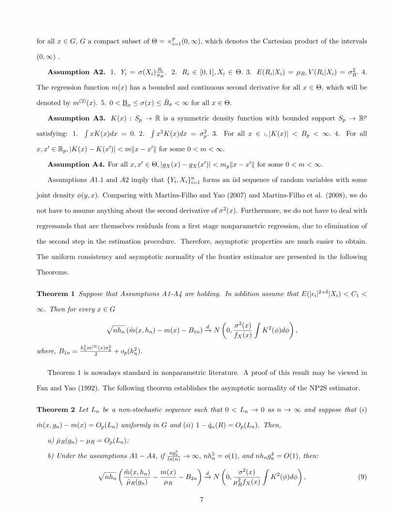
for all x ∈ G, G a compact subset of Θ = ×pi=1(0,∞), which denotes the Cartesian product of the intervals
(0,∞) .
Assumption A2. 1. Yi = σ(Xi)RiσR
. 2. Ri ∈ [0, 1], Xi ∈ Θ. 3. E(Ri|Xi) = µR, V (Ri|Xi) = σ2R. 4.
The regression function m(x) has a bounded and continuous second derivative for all x ∈ Θ, which will be
denoted by m(2)(x). 5. 0 < Bσ ≤ σ(x) ≤ Bσ <∞ for all x ∈ Θ.
Assumption A3. K(x) : Sp → R is a symmetric density function with bounded support Sp → Rp
satisfying: 1.∫xK(x)dx = 0. 2.
∫x2K(x)dx = σ2p. 3. For all x ∈ p, |K(x)| < Bp < ∞. 4. For all
x, x′ ∈ Rp, |K(x)−K(x′)| < m‖x− x′‖ for some 0 < m <∞.
Assumption A4. For all x, x′ ∈ Θ, |gX(x)− gX(x′)| < mg‖x− x′‖ for some 0 < m <∞.
Assumptions A1.1 and A2 imply that {Yi, Xi}ni=1 forms an iid sequence of random variables with some
joint density φ(y, x). Comparing with Martins-Filho and Yao (2007) and Martins-Filho et al. (2008), we do
not have to assume anything about the second derivative of σ2(x). Furthermore, we do not have to deal with
regressands that are themselves residuals from a first stage nonparametric regression, due to elimination of
the second step in the estimation procedure. Therefore, asymptotic properties are much easier to obtain.
The uniform consistency and asymptotic normality of the frontier estimator are presented in the following
Theorems.
Theorem 1 Suppose that Assumptions A1-A4 are holding. In addition assume that E(|εi|2+δ|Xi) < C1 <
∞. Then for every x ∈ G
√nhn (m(x, hn)−m(x)−B1n)
d−→ N
(0,σ2(x)
fX(x)
∫K2(φ)dφ
),
where, B1n =h2nm
(2)(x)σ2k
2 + op(h2n).
Theorem 1 is nowadays standard in nonparametric literature. A proof of this result may be viewed in
Fan and Yao (1992). The following theorem establishes the asymptotic normality of the NP2S estimator.
Theorem 2 Let Ln be a non-stochastic sequence such that 0 < Ln → 0 as n → ∞ and suppose that (i)
m(x, gn)−m(x) = Op(Ln) uniformly in G and (ii) 1− qα(R) = Op(Ln). Then,
a) µR(gn)− µR = Op(Ln);
b) Under the assumptions A1−A4, if ng5nln(n) →∞, nh5n = o(1), and nhng
4n = O(1), then:
√nhn
(m(x, hn)
µR(gn)− m(x)
µR−B2n
)d−→ N
(0,
σ2(x)
µ2RfX(x)
∫K2(φ)dφ
), (9)
7
where, B2n = Op(g2n).
Informally, assumption (2) in Theorem 2 guarantees that for appropriate values of α the sample α−quantile
of R is sufficiently close to 1 as the sample size increases. The proof of Theorem 2 is presented in Appendix 2.
Its worth to point out that Theorem 2 concerns asymptotic normality of NP2S centered at the true frontier,
ρ(·).
3.1 NP2S and NP3S comparison
Now we compare the asymptotic variances of the estimators NP2S and NP3S. Using the results stated in
Martins-Filho and Yao (2007) and the results presented in equation (9) we have the ratio between the two
aymptotic variances:
AvarNP2S
AvarNP3S=
4σ2Rµ2R(µ4(x)− 1)
, (10)
where µ4(x) = E(ε4i |Xi = x) and εi = Ri=µRσR
. Therefore, it is clear that the ratio above become smaller as µr
increases and σR decreases. Hence big µR combined with small σR values tend favorably to NP2S estimator
vis-a-vis NP3S estimator. An illustration about this point is made in the next section.
4 Monte Carlo Study
In this section we consider a simulation study to shed some light on the finite sample properties of our
estimator, henceforth referred to as NP2S100α, where α stands for the quantile order in the second step of the
proposed estimator. We consider α = 0.95, 0.96, 0.97, 0.98, 0.99, 1. For comparison purposes, we also include
in the study the local linear frontier estimator proposed in Martins-Filho and Yao (2007), referred to as NP3S,
and the well known FDH estimator. Our simulations are based on model (1), i.e., Yi = σ(Xi)Ri
σR, with p = 1.
We generate data with the following characteristics. The Xi are pseudorandom variables from a uniform
distribution with support given by [al, bu]. Ri = exp(−Zi), where Zi are pseudorandom variables from
an exponential distribution with parameter β > 0, therefore Ri has support on (0, 1]. We consider two
specifications for σ(x):
σ1(x) =√x, with x ∈ [al, bu] = [10, 100] and
σ2(x) = 3(x− 1.5)3 + 0.25x+ 1.125, with x ∈ [al, bu] = [1, 2],
which are associated with convex and non-convex production technologies. Four parameters for the expo-
nential distribution are considered: β1 = 1, β2 = 1/3. These choices of parameters produce, respectively,
8
the following values for the parameters of gR|X : (µR, σ2R) = (0.5, 0.08) and (0.75, 0.04). Two sample sizes
n = 200, 400 were used. Each experiment involved 1000 Monte Carlo replications. We evaluate the frontiers
at x0 = 55 for σ1(x) and at x0 = 1.5 for σ2(x). These values of X correspond to the 50th percentile of its
support.
The results of our simulations are summarized in figures 1-18. For figures 1-16, the thick horizontal line
inside the rectangle in each boxplot corresponds to the median of the distribution, and the rectangle height
corresponds to interquartile range. Consequently 50% of data is represented by the rectangle. The two thin
horizontal lines below and above the rectangle are the whiskers. The whiskers extend to the most extreme
data point which is no more than 1.5 times the interquartile range. Figures 1-8 give boxplots of MSE for
the frontier estimator (ρ(·)). Each boxplot is constructed from 1000 points (repetitions), where each point
corresponds to a sample draw and is calculated as the squared Euclidean distance between the estimate and
true value of ρ(·), as in equation (11). Figures 9-16 give boxplots of the frontier estimator evaluated at the
selected points mentioned above, i.e., ρ(x0). The horizontal red line represents the true value, i.e, ρ(x0).
MSE(ρ) = n−1n∑i=1
(ρ(Xi)− ρ(Xi))2. (11)
An important aspect in the implementation of our frontier estimator is bandwidth selection. We minimize
the following expression, obtained from the asymptotic analysis presented above.
ˆAMISE(h) =1
nhn
∫σ2(x)dx
∫k2(φ)dφ+
(qα
(2m(xi)Ri
2m(xi) + h2nn2γm(2)(xi)σ2k
))2 1
n
n∑i=1
m2(xi) (12)
where γ is set to be zero in all experiments. Other values in the range (0, 1/6) were considered for γ. Since
the results were similar we do not present them here. The sequence {m(Xi)}ni=1 is estimated via local linear
regression with a rule-of-thumb bandwidth as in Ruppert et al. (1995). {σ2(Xi)}ni=1 is estimated via local
linear regression of {ε2}ni=1 on {Xi}ni=1, where ε2i = (Yi − m(Xi))2, as in Fan and Yao (1998). Furthermore,
{m(Xi)}ni=1 is used to estimate Ri = Yim(Xi)
(qα
(Yi
m(Xi)
))−1. Finally, the sequence {m(2)(Xi)}ni=1 is estimated
with an ordinary least square quartic regression of {Yi}ni=1 on {Xi}ni=1.
4.1 Performance without outliers
As expected from the asymptotic results of section 3, as the sample size n increases, the boxplots in figures 1-
8 show that MSE decreases for all estimators and values for µR considered. As pointed out in subsection 3.1,
the asymptotic variance ratio between NP2S and NP3S depends on the values of µR and σR. We note that
9

for NP2S, regarding the frontier estimator, the performance in terms of MSE improves as the value of µR
increases. This pattern is most likely explained by the fact its variance is inversely proportional to µR value,
as stated in Theorem 2. In fact, when µR = 0.5, NP2S100 is similar in overall performance to NP3S, but
with an appropriate choice of α, NP2S exhibits a much smaller MSE than NP3S. In general, FDH presents
smaller distance between whiskers than NP2S and NP3S, but depending on choice of α, NP2S presents
smaller median than FDH and NP3S. In figure 17 we illustrate the behavior of the three estimators. We
emphasize that NP2S is a smooth estimator with good adjustment to the data.
4.2 Performance with outliers
In Figures 9-16 we consider samples with outliers, as explained in section 4. We see, as expected, that FDH
estimator is very sensible to outliers from the point it arises to the point where at least one observed output
becomes greater than the referred outlier. NP3S and NP2S100 are also very sensible to outliers but in a
different fashion. For both estimators an outlier tends to interfere in the positioning step, making the entire
estimated frontier to be located above of the true frontier. Nevertheless, choosing α smaller than one seems
to be a valuable strategy to overcome this problem. Indeed within this framework the outliers seem to have
no interference in the positioning step. In figure 18 we illustrate the behavior of the three estimators in the
presence of an outlier. NP2S is not affected by the outlier in that scenario.
5 Conclusion
In this paper we present a production frontier model developed by Martins-Filho and Yao (2007) that
uses Kernel regression for estimating production frontier and therefore efficiency for production units with
significant advantages when compared to DEA and FDH estimators. However, the estimation process is
made in three steps. We then propose a modification on that estimation procedure, eliminating the need of
the second step. The result is a simpler estimation procedure that retains all inherent advantages present
in the original estimator. Furthermore, we propose a generalization of the positioning step, which results in
a robust estimator. A Monte Carlo study was performed comparing three estimators: our estimator, called
NP2S; NP3S from Martins-Filho and Yao (2007); and the well known FDH estimator. The results show that
depending on choice of α, NP2S outperforms its competitors, specially when outliers are present.
10

Appendix 1: Tables and Graphics
Figure 1: Frontier I - MSE of Estimators - n = 200 - µR = 0.5
NP
2S95
NP
2S96
NP
2S97
NP
2S98
NP
2S99
NP
2S10
0
NP
3S
FD
H
0
10
20
30
40
MSE
NP
2S95
NP
2S96
NP
2S97
NP
2S98
NP
2S99
NP
2S10
0
FD
H
0
10
20
30
MSE − Except NP3S
Figure 2: Frontier I - MSE of Estimators - n = 400 - µR = 0.5
NP
2S95
NP
2S96
NP
2S97
NP
2S98
NP
2S99
NP
2S10
0
NP
3S
FD
H
0
5
10
15
20
25
MSE
NP
2S95
NP
2S96
NP
2S97
NP
2S98
NP
2S99
NP
2S10
0
FD
H
0
5
10
15
20
MSE − Except NP3S
Figure 3: Frontier I - MSE of Estimators - n = 200 - µR = 0.75
NP
2S95
NP
2S96
NP
2S97
NP
2S98
NP
2S99
NP
2S10
0
NP
3S
FD
H
0
100
200
300
400
MSE
NP
2S95
NP
2S96
NP
2S97
NP
2S98
NP
2S99
NP
2S10
0
FD
H
0
5
10
15
20
MSE − Except NP3S
Figure 4: Frontier I - MSE of Estimators - n = 400 - µR = 0.75
NP
2S95
NP
2S96
NP
2S97
NP
2S98
NP
2S99
NP
2S10
0
NP
3S
FD
H
0
50
100
150
200
MSE
NP
2S95
NP
2S96
NP
2S97
NP
2S98
NP
2S99
NP
2S10
0
FD
H
0
2
4
6
8
10
MSE − Except NP3S
11

Figure 5: Frontier II - MSE of Estimators - n = 200 - µR = 0.5
NP
2S95
NP
2S96
NP
2S97
NP
2S98
NP
2S99
NP
2S10
0
NP
3S
FD
H
0.0
0.2
0.4
0.6
0.8
1.0
1.2
1.4
MSE
NP
2S95
NP
2S96
NP
2S97
NP
2S98
NP
2S99
NP
2S10
0
FD
H
0.0
0.1
0.2
0.3
0.4
0.5
MSE − Except NP3S
Figure 6: Frontier II - MSE of Estimators - n = 400 - µR = 0.5
NP
2S95
NP
2S96
NP
2S97
NP
2S98
NP
2S99
NP
2S10
0
NP
3S
FD
H
0.0
0.2
0.4
0.6
MSE
NP
2S95
NP
2S96
NP
2S97
NP
2S98
NP
2S99
NP
2S10
0
FD
H
0.0
0.1
0.2
0.3
0.4
MSE − Except NP3S
Figure 7: Frontier II - MSE of Estimators - n = 200 - µR = 0.75
NP
2S95
NP
2S96
NP
2S97
NP
2S98
NP
2S99
NP
2S10
0
NP
3S
FD
H
0
5
10
15
MSE
NP
2S95
NP
2S96
NP
2S97
NP
2S98
NP
2S99
NP
2S10
0
FD
H
0.0
0.1
0.2
0.3
0.4
0.5
0.6
MSE − Except NP3S
Figure 8: Frontier II - MSE of Estimators - n = 400 - µR = 0.75
NP
2S95
NP
2S96
NP
2S97
NP
2S98
NP
2S99
NP
2S10
0
NP
3S
FD
H
0.0
0.2
0.4
0.6
0.8
1.0
1.2
1.4
MSE
NP
2S95
NP
2S96
NP
2S97
NP
2S98
NP
2S99
NP
2S10
0
FD
H
0.0
0.1
0.2
0.3
0.4
0.5
MSE − Except NP3S
12

Figure 9: Frontier I - Estimated frontier at selected points - Outlier at x = 55 - n = 200 - µR = 0.5
NP
2S95
NP
2S96
NP
2S97
NP
2S98
NP
2S99
NP
2S10
0
NP
3S
FD
H
16
18
20
22
24
26
28
30
Estimated frontier at x = 32.5
NP
2S95
NP
2S96
NP
2S97
NP
2S98
NP
2S99
NP
2S10
0
NP
3S
FD
H
25
30
35
Estimated frontier at x = 55
NP
2S95
NP
2S96
NP
2S97
NP
2S98
NP
2S99
NP
2S10
0
NP
3S
FD
H
25
30
35
40
45
Estimated frontier at x = 77.5
Figure 10: Frontier I - Estimated frontier at selected points - Outlier at x = 55 - n = 400 - µR = 0.5
NP
2S95
NP
2S96
NP
2S97
NP
2S98
NP
2S99
NP
2S10
0
NP
3S
FD
H
18
20
22
24
26
28
Estimated frontier at x = 32.5
NP
2S95
NP
2S96
NP
2S97
NP
2S98
NP
2S99
NP
2S10
0
NP
3S
FD
H
24
26
28
30
32
34
36
Estimated frontier at x = 55
NP
2S95
NP
2S96
NP
2S97
NP
2S98
NP
2S99
NP
2S10
0
NP
3S
FD
H
30
35
40
Estimated frontier at x = 77.5
Figure 11: Frontier I - Estimated frontier at selected points - Outlier at x = 55 - n = 200 - µR = 0.75
NP
2S95
NP
2S96
NP
2S97
NP
2S98
NP
2S99
NP
2S10
0
NP
3S
FD
H
25
30
35
40
45
Estimated frontier at x = 32.5
NP
2S95
NP
2S96
NP
2S97
NP
2S98
NP
2S99
NP
2S10
0
NP
3S
FD
H
35
40
45
50
55
60
Estimated frontier at x = 55
NP
2S95
NP
2S96
NP
2S97
NP
2S98
NP
2S99
NP
2S10
0
NP
3S
FD
H
40
45
50
55
60
65
70
Estimated frontier at x = 77.5
Figure 12: Frontier I - Estimated frontier at selected points - Outlier at x = 55 - n = 400 - µR = 0.75
NP
2S95
NP
2S96
NP
2S97
NP
2S98
NP
2S99
NP
2S10
0
NP
3S
FD
H
25
30
35
40
Estimated frontier at x = 32.5
NP
2S95
NP
2S96
NP
2S97
NP
2S98
NP
2S99
NP
2S10
0
NP
3S
FD
H
35
40
45
50
55
Estimated frontier at x = 55
NP
2S95
NP
2S96
NP
2S97
NP
2S98
NP
2S99
NP
2S10
0
NP
3S
FD
H
45
50
55
60
65
Estimated frontier at x = 77.5
13

Figure 13: Frontier II - Estimated frontier at selected points - Outlier at x = 1.5 - n = 200 - µR = 0.5
NP
2S95
NP
2S96
NP
2S97
NP
2S98
NP
2S99
NP
2S10
0
NP
3S
FD
H
4.0
4.5
5.0
5.5
6.0
6.5
7.0
Estimated frontier at x = 1.25
NP
2S95
NP
2S96
NP
2S97
NP
2S98
NP
2S99
NP
2S10
0
NP
3S
FD
H
5.0
5.5
6.0
6.5
7.0
Estimated frontier at x = 1.5
NP
2S95
NP
2S96
NP
2S97
NP
2S98
NP
2S99
NP
2S10
0
NP
3S
FD
H
5.0
5.5
6.0
6.5
7.0
7.5
8.0
Estimated frontier at x = 1.75
Figure 14: Frontier II - Estimated frontier at selected points - Outlier at x = 1.5 - n = 400 - µR = 0.5
NP
2S95
NP
2S96
NP
2S97
NP
2S98
NP
2S99
NP
2S10
0
NP
3S
FD
H
4.5
5.0
5.5
6.0
6.5
Estimated frontier at x = 1.25
NP
2S95
NP
2S96
NP
2S97
NP
2S98
NP
2S99
NP
2S10
0
NP
3S
FD
H5.0
5.5
6.0
6.5
7.0
Estimated frontier at x = 1.5
NP
2S95
NP
2S96
NP
2S97
NP
2S98
NP
2S99
NP
2S10
0
NP
3S
FD
H
5.5
6.0
6.5
7.0
7.5
8.0
Estimated frontier at x = 1.75
Figure 15: Frontier II - Estimated frontier at selected points - Outlier at x = 1.5 - n = 200 - µR = 0.75
NP
2S95
NP
2S96
NP
2S97
NP
2S98
NP
2S99
NP
2S10
0
NP
3S
FD
H
6
7
8
9
10
11
Estimated frontier at x = 1.25
NP
2S95
NP
2S96
NP
2S97
NP
2S98
NP
2S99
NP
2S10
0
NP
3S
FD
H
8
9
10
11
12
13
Estimated frontier at x = 1.5
NP
2S95
NP
2S96
NP
2S97
NP
2S98
NP
2S99
NP
2S10
0
NP
3S
FD
H
7
8
9
10
11
12
13
Estimated frontier at x = 1.75
Figure 16: Frontier II - Estimated frontier at selected points - Outlier at x = 1.5 - n = 400 - µR = 0.75
NP
2S95
NP
2S96
NP
2S97
NP
2S98
NP
2S99
NP
2S10
0
NP
3S
FD
H
4.0
4.5
5.0
5.5
6.0
6.5
7.0
Estimated frontier at x = 1.25
NP
2S95
NP
2S96
NP
2S97
NP
2S98
NP
2S99
NP
2S10
0
NP
3S
FD
H
5.0
5.5
6.0
6.5
7.0
Estimated frontier at x = 1.5
NP
2S95
NP
2S96
NP
2S97
NP
2S98
NP
2S99
NP
2S10
0
NP
3S
FD
H
5.0
5.5
6.0
6.5
7.0
7.5
8.0
Estimated frontier at x = 1.75
14

Figure 17: Estimated frontier - Example - n = 400
●
●
●
●
●
●
●
●
●
●
●
●
●
●
●
●
●
●
●
●
●●
●
●
●
●
●
●
●
●
●
●
●
●
●
●
●
●●
●
●
●
●
●
●
●
●
●
●
●
●
●
●
●
●
●
●
●●
●
●
●
●
●●
●●
●
●
●
●
●
●
●
●
●
●
●
●
●
●
●
●
●
●
●
●
●
●
●
●
●
●
●
●
●
●
●
●
●
●
●
●
●
●
●
●
● ●
●
●
●
●
●
●
●
●
●●
●
●
●
●
●
●
● ●
●
●
●
●
●
●
●
●
●
●
●
●
●
●
●
●
●
●
●
●
●
●
●
●
●
●
●
●
●
●
●
●
●
●
●
●●
●
●
●
●
●
●
●
●●
●
●
●●
●
●
●
●
●
●
●
●
●
●
●
●
●
●
●
●
●
●
●
●
●
●
●
●
●
●
●
●
●
●
●
●
●
●
●
●
●●
●
●
●
●
●
●
●
●●
●
●
●
●
●
●
●
●
●
●
●
●
●
●
●
●
●
●
●
●
●
●
●
●
●
●
●
●
●
●
●
●
●
●
●
●
●
●
● ●
●
●
●
●
●
●
●
●
●
●
●
●
●
●
●
●
●
●
●
●●
●
●
●
●
●
●
●
●
●
●
●●
●
●
●
●
●
●
●
●
●
●
●
●
●
●
●
●
●
●
●
●
●●
●●
●
●
●
●
●
●
●
●
●
●
●
●
●
●
●
●
●
●
● ●
●
●
●●
●
●
●
●
●
●
●●
●
●
●
●●●
●
●
●
●●
●
●●
●
●
●
●
●
●
●
●
●
●
●
●
●
●
●
●
●
●
●
●
●
●
●
●
●
●
●
●
●
●
●
●
●
20 40 60 80 100
010
2030
40
x
y
TrueNP2S98
FDHNP3S
(a) Frontier I - µR = 0.5
●
●
●
●
●
●
●
●
●
●
●
●
●●
●
●●
●●
●
●
● ●
●
●
●
●
●
●
●
●
●
●
●
●
●●
●●
●
●
●
●
●
●
●
●●
●
●
●
●
●●
●
●
●
●
●
●
●●
●
●
●
●
●
●
●
●
●
●
●●
●
●
●
●
●
●
●
●
●
●
●
●●
●
●
●
●
●
●
●
●
●
●
●
●
●
●
●
●●●
●
●
●
●
●
●
●
●
●
●
●
●
●
●
●
●
●
●
●
●
●
●
●
●●
●
●
●●
●
●
●
●
●
●
●
●
●
●
●
●
●
●
●
●
●
●
●
●
●
●
●
●
●
●
●
●
●
●
●
●
●
●
●
●
●
●
●
●
●
●
●
●
●
●
●
●
●●
●
●
●
●
●
●
●
●
●
●
●
●
●
●●
●
●
●
●
●
●
●
●
●
●
●
●
●
●
●
●
●
●
●
●
●
●
●
●
●
●
●
●
●
●
●
●
●
●
●
●
●
●
●
●
●
●●
●
●
●
●
●●
●
●
●
●
●
●
●
●
●
●
●
●
●
●
●
●
●
●
●
●
●
●
●
●
●
●
●
●
●
●
●
●
●
●●
●
●
●
●
●
●
●
●
●
●
●
●
●
●
●
●
●
●
●
●
●
●
●
●●
●
●
●●
●
●
●
●
●
●
●
●
●
●●
●
●
●
●
●●
●
●
●
●
●
●
●
●
●
●
●
●
●
●
●
●
●
●
●
●
●
●
●
●
●
●
●
●
●●
●
●
●
●
●
●
●
●
●●
●
●
●
●
●
●
●
●
●
●
●
●
●
●
●
●
●
●
●
●
●
●
●
●
●
●
●
●
●
●
●
20 40 60 80 100
010
2030
4050
x
y
TrueNP2S98
FDHNP3S
(b) Frontier I - µR = 0.75
●
●
●
●
●
●
●
●
●
●
● ●
●
●
●
●
● ●
●
●
●
●
●
●
●
●
●
●
●
●●
●
● ●
●
●
●●
●
●
●
●
●
●
●
●
●
●
●
●
●●
●
●
●
●
●
●
●
●
●
●
●
●
●
●
● ●
●
●
●
●
●
●
●
●
●
●
●
●
●
●
●
●
●
●
●
●
● ●
●
●
●
●
●
●
●
●●
●
●
●
●
●
●
●
●
●
●
●
●
●
●
●
●
●
●
●
●
●
●
●●
●
●
●
●
●
●
●
●
●
●
●
●
●
●●
●●
●
●
●
●
●
●
●
●
●
●
●●
●
●
●
●
●
●
●
●
●
●
●
●
●
●
●
●
●
●
●
●
●
●
●
●
●
●
●
●
●
●
●
●
●
●
●
●
●
●
●●
●
●
●
●
●
●
●
●
●
●
●
●
●
●
●●
●●
●
●
●
●
●
●
●
●
●
●
●
●
●
● ●●
●
●
●
●●
●
●●
●
●
●
●
●
●
●
●
●
●
●
●
●
●
●
●
●
●
●
●
●
●
●
●
●
●
●●
●
●
●
●
●
●
●
●
●
●
●
●
●
●
●
●
●
●●
●●
●
●
●
●
●
●
●
●
●
●
●
●
●
●
●
●
●
●●
●
●
●●
●
●
●
●
●
●
●
●
●
●
●
●
●
●
●
●
●
●
●
●
●
●
●
●
●
●●
●
●
●
●
●
●
●
●●
●
●
●
●
●
●
●●
●
●
●
●
●
●
●
●
●
●
●
●
●
●
●
●
●
●
●
●
●
●
●
●
●
●
●
●
●
●
●
●
●
●
●
●●
●
● ●
●
●
●
●
●
●
●
●●
●
1.0 1.2 1.4 1.6 1.8 2.0
02
46
x
y
TrueNP2S98
FDHNP3S
(c) Frontier II - µR = 0.5
●
●
●
●
●
●
●
●
●
●
●
●
●
●
●
●●
●●
●
●●
●
●
●
●
●
●
●
●
●
●
●
●
●
●
●
●
●
●
●
●
●
●
●
●
●
●
●
●
●
●
●
●
●
●
●
●
●
●
●
●
● ●
●
●
●
●
●
●
●
●
●
●
●
●
●
●
●
●
●
●
●
●
●
●
●
●
●
●
● ●
●
●
●
●
●
●
●
●
●●
●
●
●
●
●
●
●
●
●●
●
●
●
●
●
●
●
●
●
●
●
●
●●
● ●
●
●
●
●
●
●
●
●
●
●● ●
●●
●
●
●
●
●
●
●
●●
●
●
●
●
●
●
●
● ●
●
●
●
●
●
●
●
●
●
●
●
●
●
●
●●
●
●
●
●
●
●
●●
●
●
● ●
●●
●
●
●
●
●
●
●
●
●
●
●
●
●●
●
●
●
●
●
●
●
●●
●
●
●
●
●
● ●
●
●
●
●
●
●●
●
●
●●
●
●
●
●
●
●
●
●
●
●
●
●
●
●
●
●
●
●
●
●
●
●
●
●
●
●●
●
●
●
●
●
●
●
●
●
●
●
●
●
●
●●
●
●
●
●
●
●
●
●
●●
● ●
●
●
●
●
●
● ●
●
●
●
●
●
●
●
●
●
●
●
●
●
●
● ●
●
●
●
●
●
●
●
●● ●
●
●
●
●
●
●
●
●
●●
●
●
●
●
●
●
●
●
●
●
●
●
●
●
●
●
●
●
●
●
●
●
●
●
●
●
●
●
●
●
●
●
●
●
●
●
●
●
●
●
●
●
●
●
●
●
●
●
●
●
●
●
●
●●
●
●
●
●
●
●
●
●
●
●
●
●
●
●
●
●
1.0 1.2 1.4 1.6 1.8 2.0
02
46
810
x
y
TrueNP2S98
FDHNP3S
(d) Frontier II - µR = 0.75
15
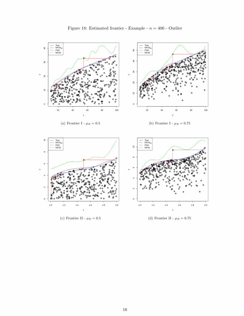
Figure 18: Estimated frontier - Example - n = 400 - Outlier
●
●
●
●
●●
●
●
●
●
●●
●
●
●●
●
●
●
●
●
●
●
●
●
●
●
●
●●
●
●
●
●
●
●
●
●
●
●●
●
●
●
●
●
●
●
●
●
●
●
●
●● ●
●
●
●
●
●
●
●
●
●
●
●●
●
●
●
●
●
●
●
●●
●
●
●
●
●
●
●
●
●
●
●
●
●
●
●
●
●
●
●
●
●
●
●
●
●
●
●
●
●
●
●
●
●
●
●
●
●
●
●
●
●
●
●
●
●
●
●
●
●
●
●
●
●
●
●
●
●
●
●
●
●
●
●
●
●
●●
●
●
●
●●
●
●
●
●
●●
●
●
●●
●
●
●
●
●
●
●
●
●
●
●
●
●
●
●
●
●
●
●
●
●
●
●
●
●
●
●
●
●
●
●
●
●
●
●
●
●
●
●
●
●●
●
●
●
●
●
●
●
●
●
●
●
●
●
●
●
●
●
●
●
●
●
●●
●
●
●
●
●
●
●
●
●
●
●
●
●
●
●
●
●
●
●
●
●
● ●
●
●
●
●
●
●
●●
●
●
●
●
●
●
●
●
●
●
●
●
●
●
●
●
●
●
●
●
●
●
●
●
●
●
●
●
●
●
●
●
●
●
●
●
●
●
●
●
●
●
●
●
●
●
● ●
●
●
●
●
●
●
●
●
●
●
●
●
●
●
●
●
●
●
●
●
●
●●
●
●
●
●
●
●
●
●●
●
●
●
●
●
●
●
●
●
●
●
●
●
●
●
●
●
●
●
●
●
●
●
●
●●
●
●
●
●
●●
●
●
●
●
●
●
●
●
●
●
●
●
●
●
●
●
●
●
●
● ●
●
●
●
●
●
●
●
●
●
●
●
●
20 40 60 80 100
010
2030
40
x
y
TrueNP2S98
FDHNP3S
(a) Frontier I - µR = 0.5
● ●
●
●
●
●
●
●
●
●
●
●
●
●
●
●
●
●
●
●
●
●
●
●●
●
●
●
●
●
●
●
●
●
●
●
●
●
●
●
●
●
●
●
●
●
●
●
●
●
●
●
●●●
●
●
●
●
●
●
●
●
●
●
●
●
●●
●
●
●
●
●
●
●
●
●
●●
● ●
●
●
●
●
●
●
●
●
●●
●
●
●
●
●
●
●
●
●
●
●
●
●
●
●
●
●
●
●
●
●
●
●
●
●
●
●
●
●
●
●
●
●
●
●
●
●
●
●
●
●
●
●
●
●
●
●● ●
●
●
●
●
●
●
●
●
●
●
●
●
●
●
●
●
●
●
●
●
●
●
●
●
●
●
●
●
●
●
●
●
●
●
●●
●
●
●
●
●
●
●
●
●
●
●
●●●
●
●
●
●
●
●
●
●
●
●
●
●
●
●
●
●
●
●
●
●
●
●
●
●
●
●
●
●
●
●
●
●
●
●
●
●
●
●
●
●
●
●
●
●
●
●
●●
●
●
●
●●
●
●
●
●●
●
●
●
●
●
●
●●
●●
●
●●
●
●
●
●
●
●
●
●
●
●
●
●
●
●
●
●
●
●
●
●
●
●
●
●●
●
●
●
●
●
●
●
●● ●
●
●
●
●
●
●
●
●
●●
●
●
●
●
●
●
●
●
●
●
●
●●
●
● ●
●
●
●●
●
●
●●
●●
●
●
●
●
●
●
●
●
●
●
●
●
●●
●
●
●
●
●
●
●
●
●
●
●
●
●
●
●
●
●
●
●
●
●
●
●
●
●
●
●
●
●
●
●
●
●
●
●
●
● ●
●
●
●
●
●●
●
●
●
●
●●
●
●
●
20 40 60 80 100
010
2030
4050
x
y
TrueNP2S98
FDHNP3S
(b) Frontier I - µR = 0.75
●
●
●
●
●
●
●
●
●
●
●
●
● ●
●
●
●
●
●
●
●
●
●
●
●
●
●
●
●
●
●
●
●
●
●
●
●
●
●
●
●
●
●
●
●
●
●
●
●●
●
●
●
●
●
●
●
●
●
●
●
●
●
●
●
●
●
●
●
●
●
●
●●
●
●
●
●
●
●
●
●
●
●
●
● ●
●
●
●
●●
●
●
●
●●
●
●
●
●
●
●
●
●
●●
●
●
●
●
●
●
●
●
●
●
●
●
●
●
●
●
●
●
●
●
●
●
●
●
●
●
●
●
●●
●
●
●●
●
●
●
●
●
● ●
●
●
●
●
●
●
●
●
●●
●
●
●
●
●
●
●
●
●
●
●
●
●
●
●
●
●
●
●
●
●
●
●
●
●
●
●
●
●
●●
●
●
●●
●
●
●
●
●
●
●
●●
●
●
●
●●
●
●
●
●
●
●●
●
●
●
●●
●
●
●●
●
●
●
●
●
●
●
●
●
● ●
●
●
●
●
●
●
●
●
●●
●
●
●
●
●
●
●
●
●
●
●
●●
●
●
●
●
●
●
●●
●
●
●
●
●
●
●
●
●
●
●
●
●
●
●
●
●
●
●
●
●
●
●
●
●
●
●
●
●
●
●●
●
●
●
●
●
● ●
●
●
●
●
●
●
●
●
●
●
●
●
●
●
●
●●
●
●
●
●
●●
●
●
●
●
●
●
●
●
●
●
●
●
●
●
●
●
●
●
●
●
●
●
●
● ●
●
●
● ●
●
●●
●
●
●
●
●
●
●
●
●
●
●
●
●
●
●
●
●
●
●
●
●
●
●
●
●●
●
●
●
●
●
●
●
●
●
●
●
●
●●
●
1.0 1.2 1.4 1.6 1.8 2.0
02
46
810
x
y
TrueNP2S98
FDHNP3S
(c) Frontier II - µR = 0.5
●●
●
●
●
●
●
●
●● ●
●
●●
●
● ●
●
●
●
●
● ●
●
●
●
●
●
●
●
●
●
●
●
●
●
●●
●
●●
●
●
●
●
●●
●
●
●
●
●
●
●
●
●
●
●
●
●
●
●
●
●
●
●
●
●
●
●
●
●
● ●
●
●
●
●
●●
●
●
●
●
●
●
●
●
●
●
●
●
●
●
●
●
●
●
●
●
●
●●
●
●●
●
●
●
●
●
●
●
●
●●
●●
●
●
●
●
●
●
●
●
●
●
●
●
●
●
●
●
●●
●
●
●
●●
●
●
●
●
●
●
●
●●
●
●
●
●
●
●
●
●
●
●
●
●
●
●
●
●
●
●
●
●
●
●
●
●
●
●
●
●
●●●
●
●
●
●
●
●
●
●
●
●
●
●
●
●
●
●
●
●
●
●
●●
●
●●
●
●
●
●
●
●
●
●
● ●
●
●
●
●
●
●
●
●
●
●
●
●
●●
●
●
●
●
●
●
●
●
●
●
●
●
●●
● ●
●
●
●
●
●●
●
●
●
●
●
●●
●
●
●
●
●
●
●
●
●
●
●
●
●
● ●●
●●
●
●
●●
●
●
●
●
●
●
●
●
●
●
●●
●
●
●
●
●
●
●
●
●
●
●
●●
●
●
●
●
●
●
●
●
●●
●
●
●
●
●
●
●
●
●
●
●
●●
●
●
●
●
●●
●
●
●
●
●●
●
●
●●
●
●
●
●
●
●
●
●
●
●●
●
●
●
●●
●
●●
●
●
●
●
●
●
●
●
●
●
●
●
●
●
●
●
●
●
●
●
●
●
●
●
●
●
●
●
●
●
●
●●
●
●
●
1.0 1.2 1.4 1.6 1.8 2.0
02
46
810
x
y
TrueNP2S98
FDHNP3S
(d) Frontier II - µR = 0.75
16

6 Appendix 2: Proofs
Proof of Theorem 2: To prove Theorem 2 we first note that Martins-Filho and Yao (2007) get after two
steps σ(Xt, hn) which is in fact σRρ(Xt, hn). Then, to obtain asymptotic normality of the estimated frontier,
ρ(.), they divided σ(x, hn) by sR(gn) and combine their Theorem 1 and their Theorem 2 part (a) to achieve
the desired result. In our case, after one step, we get m(Xi, hn) which is in fact µRρ(Xi, hn). Therefore, to
obtain the result claimed in our Theorem 2 part (b), we just need to combine the results from our Theorem
1 and our Theorem 2 part (a).
To prove Theorem 2 part (a), we use the same argument presented in the proof of Theorem 2 part (a)
of Martins-Filho and Yao (2007); but substituting in their proof σ(Xt) by m(Xi) as well as σ(Xt, gn) by
m(Xi, gn), and σR by µR as well as sR(gn) by µR(gn).
For a proof of part (b), we note that
√nhn
(m(x,hn)µR
− m(x)µR− B1n
µR
)≡√nhn
(m(x,hn)µR(gn)
− m(x)µR− m(x, hn)
(1
µ(gn)− 1
µR
)− B1n
µR
).
From Theorem 1 we have
√nhn
(m(x,hn)µR
− m(x)µR− B1n
µR
)d−→ N
(0, σ2(x)
µ2RfX(x)
∫K2(φ)dφ
),
and from Theorem 2 part (a), provided that ng5nln(n) →∞ we have that µR(x, hn)(µR(gn)−1−µR−1) = Op(g
2n).
Hence, given that nh5n → 0 and nhng4n = O(1)
√nhn
(m(x, hn)
µR(gn)− m(x)
µR−B2n
)d−→ N
(0,
σ2(x)
µ2RfX(x)
∫K2(φ)dφ
),
where, B2n = Op(g2n). 2
17

7 References
Aigner, D., C.A.K. Lovell and P. Schmidt, 1977, Formulation and estimation of stochastic frontiers produc-
tion function models. Journal of Econometrics 6, 21-37.
Aragon, Y., Daouia A., and Thomas-Agnan, C. 2005, Nonparametric Frontier Estimation: a conditional
quantile-based approach. Econometric Theory, 21, 2005, 358-389.
Cazals, C., J.-P. Florens and L. Simar, 2002, Nonparametric frontier estimation: a robust approach. Journal
of Econometrics 106, 1-25.
Charnes, A.,W. Cooper and E. Rhodes, 1978, Measuring the efficiency of decision making units. European
Journal of Operational Research 2, 429-444.
Deprins, D., L. Simar and H. Tulkens, 1984, Measuring labor inefficiency in post offices, in: M. Marchand, P.
Pestiau and H. Tulkens, (Eds.), The performance of public enterprises: concepts and measurements. North
Holland, Amsterdam.
Fan, J., 1992, Design-adaptive Nonparametric Regression. Journal of the American Statistical Association,
Vol. 87, No. 420, 998-1004.
Fan, J. and I. Gijbels, 1995, Data driven bandwidth selection in local polynomial fitting: variable bandwidth
and spatial adaptation. Journal of the Royal Statistical Society, B 57, 371-394.
Fan, J. and Gijbels, I., 1996, Local Polynomial Modelling and Its Applications. London: Chapman and Hall.
Fan, J., and Q. Yao, 1998, Efficient estimation of conditional variance functions in stochastic regression.
Biometrika 85, 645-660.
Farrell, M., 1957, The measurement of productive efficiency. Journal of the Royal Statistical Society A 120,
253-290.
Gijbels, I., E. Mammen, B. Park and L. Simar, 1999, On estimation of monotone and concave frontier func-
tions. Journal of the American Statistical Association 94, 220-228.
Korostelev, A. P., L. Simar and A. B. Tsybakov, 1995, Efficient estimation of monotone boundaries. Annals
of Statistics 23, 476-489.
Martins-Filho, C. and Yao, F., 2007, Nonparametric frontier estimation via local linear regression. Journal
of Econometrics.
Martins-Filho, C., Torrent, H., Ziegelmann, F., 2013, Nonparametric Frontier Estimation: Using Local Ex-
ponential Regression for Conditional Variance. Brazilian Review of Econometrics.
18

Park, B., L. Simar and Ch. Weiner, 2000, The FDH estimator for productivity efficient scores: asymptotic
properties. Econometric Theory 16, 855-877.
Seifford, L., 1996, Data envelopment analysis: the evolution of the state of the art (1978-1995). Journal of
Productivity Analysis 7, 99-137.
Silverman, B.W., 1986, Density estimation for statistics and data analysis. Chapman and Hall, London.
Ziegelmann, F. A., 2002, Nonparametric estimation of volatility functions: the local exponential estimator.
Econometric Theory, 18: 985-992.
19


