499
The Towers Perrin Global Capital Market Scenario Generation System
John M. Mulvey’) and A. Eric Thorlacius’)
Abstract Financial management requires a systematic approach for generating scenarios of future capital markets. Today’s global environment demands that the scenarios link the economies of individual countries within a common framework. We describe a global scenario system, developed by Towers Perrin, based on a cascading set of stochastic differential equations. The system applies to financial systems for pension plans and insurance companies throughout the world. A case study illustrates the process.
La gestion tinanciere demande une approche systematique pour gbnerer des scenarios pour les marches futurs des capitaux. L’environement global de nos jours demande que les scenarios relient les economies des pays darts une approche commune. Nous d6crivons un model de scenario global developpt5 par Towers Perrin base sur une cascade d’t?quation differentielles al6atoires. Le model s ‘applique aux portefeuilles de pension et d ‘assurance dans le monde entier. Un example et utilis6 pour illustrer le model.
Keywords Asset-liability management, economic forecasting, pension planning, insurance industry.
Department of Civil Engineering and Operations Research, Princeton University, Princeton, NJ 08542 (USA); Tel: + l-609-258 5423, Fax: + l-609-258 3791, E-mail: [email protected] Towers Pen-in, Centre Square East, 1500 Market Street, Philadelphia, PA 191024790 (USA); Tel: + 1-215-246 7508, Fax: + 1-215-246 7576.
500
1.0 Introduction
Towers Perrin, one of the world’s largest actuarial consulting companies, employs a
capita1 market scenario generation system, called CAP:Link, for helping its clients in
understanding the risks and opportunities relating to capita1 market investments. The
system produces a representative set of individual simulations - typically 500 to 1000.
Each scenario contains key economic variables such as price and wage inflation, interest
rates at different maturities (real and nominal), stock dividend yields and growth rates,
and exchange rates through each year for a period of up to 20 years. We mode1 returns
on asset classes and liability projections consistent with the underlying economic fac-
tors, especially interest rates. The economic variables are simultaneously determined
for multiple economies within a common global framework. Long-term asset and li-
ability management is the primary application.
A variety of stochastic optimization models exist for multi-period financial analysis.
Prominent examples include: Berger and Mulvey (1995), Boender (1995), Cariiio et al.
(1994), Dempster (1996) and Wilkie (1995). These systems are designed around a set
of simplifying assumptions that depend upon the target application. Stochastic financial
simulations fall within three broad categories:
Prediction - These systems forecast short-term market movements. It is not necessary
to achieve perfect accuracy, only enough to realize an expected profit. Hedge funds and
other leveraged traders often employ computerized prediction systems. The desired
output is a single scenario for next period’s economic variables. Prediction becomes
more challenging as the length of the planning period increases since markets adapt to
changing conditions. Most trading systems consider short-term horizons --- hours or
days. Hence, validity can be ascertained by historical back-testing the recommended in-
vestment strategies.
Pricing - Derivative securities often possess complex price relationships with capital
market variables, such as the pattern of interest rates movements. By capturing this in-
501
formation via models where the end-of-period outcome of the various alternatives can
be compared through a set of scenarios, we can check for consistency in pricing. It of-
ten applies in the creation of custom deals wherein the parties exchange specific market
risks. The arbitrage-free condition is important since the existence of arbitrage opportu-
nities suggests inconsistency with traded securities.
Risk Analysis - This activity evaluates the potential rewards and risks of various in-
vestment and liability management strategies. By managing investment decisions and
considering liability issues as part of an integrative financial picture, significant risks
can be avoided and opportunities for enhanced return created by accepting risks which
may be more severe to other investors - due to a different liability structure. Viewing
investment choices from the perspective of their ability to meet specified liability objec-
tives changes the relative riskiness of investment alternatives. As an example, long term
bonds which may be relatively risky to some short term investors are attractive to a pen-
sion plan with a specific long-term and fixed horizon. In contrast, when the liability
structure depends upon inflation, index linked bonds becomes a conservative asset cate-
gory. Alternatives like cash may be risky in this context because the inflation adjusted
value at a long term horizon is uncertain.
Several obstacles stand in the way of successful applications of asset and liability man-
agement. First, industries, such as insurance and banks, have been controlled by regula-
tions and legal restrictions, causing difficulty in modeling the dynamic aspects of the
key economic variables with reference to the market values of assets and liabilities. As
regulations and rules change across the globe, however, economic issues gain in impor-
tance, and as a consequence, the ability to model the stochastic elements improves. A
second receding obstacle is the computational resources needed to solve the multi-
period financial planning model. Today, powerful workstations, PCs, and efficient al-
gorithms are available for solving financial optimization problems; for example, see
Mulvey, Armstrong and Rothberg (1995).

502
CAP:Link, developed primarily for asset liability management (ALM), entails an ongo-
ing process of information gathering, evaluation and action in order to maximize the or-
ganization’s wealth over time. Asset and liability mixtures complicate the situation. It
is common to either over emphasize the liability matching investment alternatives (via
immunization or similar approaches) or to focus on expected return and volatility of as-
set return. The investor must balance expected asset return and confidence in meeting
liability obligations. A case study (section 4) offers more ideas on asset liability man-
agement and CAP:Link’s role in financial planning. In brief, CAP:Link portrays the
relationships between modeled variables, their interactions through time, and the ranges
and distributions of outcomes in a consistent manner. Investment strategies and as-
sumption setting can be evaluated by means of representative scenarios.
The rest of the paper is organized as follows. The next section describes the overall
structure of global CAP:Link. We emphasize the relationship of the single country
modules within a global setting. Much experience has been gained by implementing
CAP:Link in over 14 countries throughout North America, Europe and Asia. The global
design links the single country modules in a consistent fashion. In addition, we model
currencies between all pairs of countries, as described in section 2.4. Section 3 takes up
some implementation issues, including the critical assumption setting and calibration
elements. We present a case study in section 4 in which the scenarios form the basis for
an analysis of a large pension plan. We show the process for evaluating the a pension
plan’s health from several perspectives. Last, in section 5, we mention ideas for future
work.
2.0 Model Structure
The global CAP:Link system forms a linked network of single country modules. Figure
1 illustrates the overall structure for four countries. The three major economic powers -
the United States, Germany, and Japan -- occupy a central role, with the remaining
countries designated as home or other countries. We assume that the other countries are
affected by, but do not impact, the economies of the three major countries. The basic

503
stochastic differential equations are identical in each country, although the parameters
reflect unique characteristics of each particular economy. Notice the direction of Figure
1 arcs. Additional countries can be readily included in the framework by increasing the
number of other countries.
Figure 1: Triad of cornerstone countries and other countries. Direction of arcs shows the flow of infor- mation in the model.
Within each country, the basic economic structure is illustrated in Figure 2. Variables at
the top of the structure influence those below, but not vice-versa. This approach eases
the task of calibrating parameters. The ordering does not reflect causality between eco-
nomic variables, but rather captures significant co-movements. Linkages across coun-
tries occur at various levels of the model -- for example, interest rates and stock returns.
These connections will be discussed later. Roughly, the economic conditions in a single
country are more or less affected by those of its neighboring countries and by its trading
partners. The degree of interaction depends upon the country under review.
The structure is based on a cascade format - each sub-module within the system is pos-
sibly affected by modules above and equal to that module. Briefly, the first level con-
sists of short and long interest rates, and price inflation. Interest rates are a key attribute
in modeling asset returns and especially in coordinating the linkages between asset re-
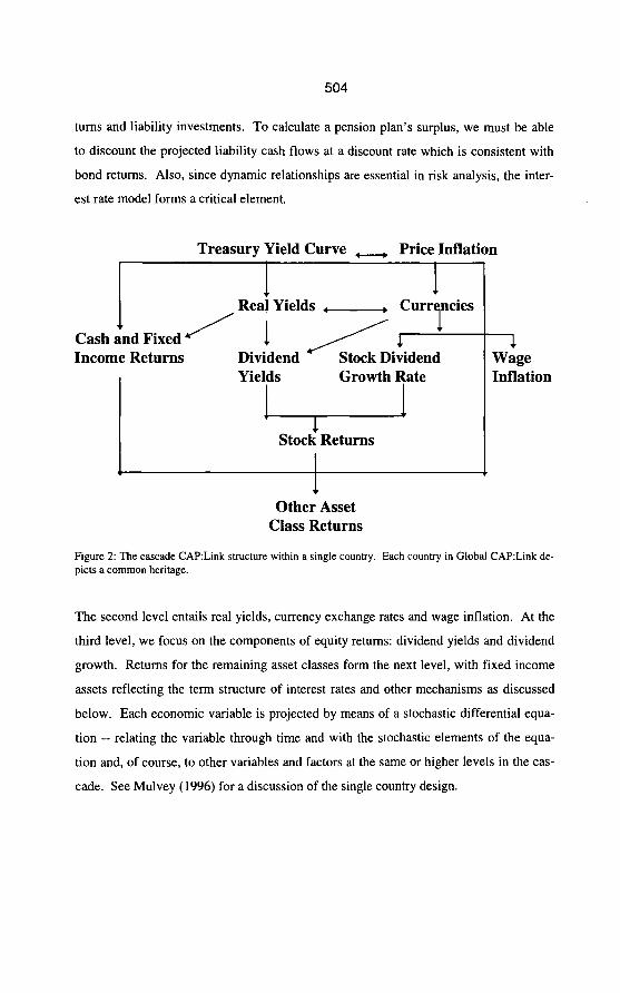
504
turns and liability investments. To calculate a pension plan’s surplus, we must be able
to discount the projected liability cash flows at a discount rate which is consistent with
bond returns. Also, since dynamic relationships are essential in risk analysis, the inter-
est rate model forms a critical element.
Treasury Yield Curve +------, Price Inflation
I I Real Yields .-, Curr ncies
Cash &d Fixed/ 1 Income Returns Dividend
/ Jr Stock Dividend
Yields Growth Rate
1 Stock Returns
. .
Other Asset Class Returns
1 Wage Inflation
Figure 2: The cascade CAP:Link structure within a single country. Each country in Global CAP:Link de- picts a common heritage.
The second level entails real yields, currency exchange rates and wage inflation. At the
third level, we focus on the components of equity returns: dividend yields and dividend
growth. Returns for the remaining asset classes form the next level, with fixed income
assets reflecting the term structure of interest rates and other mechanisms as discussed
below. Each economic variable is projected by means of a stochastic differential equa-
tion -- relating the variable through time and with the stochastic elements of the equa-
tion and, of course, to other variables and factors at the same or higher levels in the cas-
cade. See Mulvey (1996) for a discussion of the single country design.

505
2.1 Interest Rate Generation
The path of spot interest rates for non-callable government obligations sits at the top of
the cascade. Yield curve values are determined in a sequential fashion. First, the short
and long spot rates are computed by a variant of the two factor Brennan Schwartz ap-
proach (1982). At its simplest within a country, we assume that long and short interest
rates link together through a correlated white noise term and by means of a stabilizing
term which keeps the spread between the short and long rates under control. In addition,
we link the white noise terms across selected countries. The requisite equations are
listed below. All elements are indexed as vectors across the target countries.
Short rate: dq =hPu -q) dt +hPw q, 1, lb pu ,pt)dt +.Mt) dzl (1) Long rate: dlt =f& -It) dt +fsCr,, ,rb 1, lb pwpt)dt +f6(rf) dZ2 (2)
where ru is the normative level of short interest rates,
rt is the level of interest rates at time t,
Zr, is the normative level of long interest rates,
it is the level of rates at time t,
pu is the normative level of inflation andpt is the level at time t, and
h, ***, f6 are vector functions that depend upon various economic factors up to
period t.
The random coefficient vectors -- dZz and dZ2 -- depict correlated Wiener terms.
These two vector diffusion equations provide the building blocks for the remaining spot
interest rates, and the full yield curve. At any point t, the mid-rate is a function of the
short and long rates. Other points on the spot rate curve are computed by smoothing a
double exponential equation for the spot rate of interest.
2.2 Inflation Generation
The price inflation routine lies aside the interest rate model in the cascade structure.
Price inflation at period t depends upon price inflation in previous time periods and on
the current yield curve. Again, the economic time series is modeled as a diffusion proc-
ess. Controls are placed on internal parameters and interest rates -- the yield curve. The

506
key diffusion equations are shown below. As before, these equations index over the in-
dividual countries (as vectors):
Price inflation: dpt =h dq +fs bw pt, rw rb lw It, dt +fdvt ) dZ3 (3)
Stochastic volatility: d vt = f,o (v, - vt ) dt + f,,( vt ) dZI (4)
where vu is the normative level of inflation volatility and vt is the level at time t, and
A --*, f,, are vector functions that depend upon various economic factors up to
period t.
The random coefficient vectors -- dZ3 and dZ4 -- depict white noise terms consisting of
parts reflecting local and global effects. In the US and other economies, price inflation
is more volatile than interest rates. Part of the explanation is the lack of a traded secu-
rity representing inflation’. Also, the volatility of inflation persists. Once inflation
volatility increases, for example, through a economic shock such as the oil crisis, it re-
mains high for some time before settling down to a more normal level. Modeling sto-
chastic volatility requires a second diffusion equation (4).
Next in the cascade is wage inflation. This parameter connects to price inflation in a
lagged and smoothed fashion. Wages are relatively slow to react to changes in price in-
flation, but they inevitably follow over time. Pension plan liabilities are directly tied to
wage inflation.
2.3 Real Yields
Real interest rates are defined in two distinct ways. First, we equate real interest rates
with the spread of nominal interest rates to current inflation. Some economies provide
explicit real return bonds as traded securities issued by government bodies, for instance,
index linked bonds in the UK and Canada. These securities provide a specified return
over inflation for a fixed period. Real returns in a net of inflation framework are
equivalent to nominal yields in a total return context. Regulatory bodies in some coun-
tries set valuation by discounting with real yield rates. Real yields relate to the move-
ment of interest rates, current inflation, as well as expectations for future inflation. The
equation for long term real yields is shown below:

507
d&=fn(k, kb 1, lbPwPt)dl +fn( ~wpb k, k, 1, It, dt +fi&) dzs (5)
where k, is the normative level of real yields and kt is the level at time t, and
fl2, . . . . fir are vector functions that depend upon various economic factors up to
time t.
The random coefficient vector dZs depict correlated Wiener terms. To derive the
complete real yield curve, we calculate a short-term real yield based on short nominal
rates and current inflation -- providing two points on the curve. Remaining points are
determined by interpolating the structure of the nominal interest rate curve.
2.4 Currencies
Several complication issues arise when modeling currency exchange rates. First, cur-
rencies must enforce the arbitrage free condition among spot exchange rates and among
forward rates with differential interest rates. The second issue involves symmetry and
numeraire independence; we must create a structure in which the distribution of cur-
rency returns from country A to B has the same distribution as returns from B to A.
Both issues limit the form of the currency exchange models, especially when integrating
three or more currencies. To avoid these problems, we focus on the strength of each
country’s currency. Exchange rate follows as the ratio between the strengths of any two
counties. See Mahieu and Schotman (1994) for a similar approach to currencies. The
absolute strength of any currency is a notional concept; the relative levels reflect the dif-
ference in the exchange rates.
The exchange rate equation between country i and j becomes the ratio: si / sj , where si
and sj reflects the strength of currency i and j, respectively.
The equation describing the development of the individual currency strengths follows:
dq=fis (rw rbpwpbppt) dt +fia d& (6)
where
ppt is the average cost of goods in foreign countries relative to domestic cost and

508
fls and fia are vector functions that depend upon various economic factors up to
period t.
The random coefficient vector dzg depicts correlated Wiener terms. Addressing rela-
tive currency strengths involves not only current economic conditions but also historical
trends. For example, an important long-term relationship is purchase power parity
(PPP). The per term depicts the pattern of inflation and currency movements in the
projection up to time t. Purchase power parity states that exchange rates should keep
pace with price inflation. Currency is an intermediary for the ultimate exchange of
goods and services. The inflation differential between two economies approximates the
change in the relative cost of goods in each country; currency being conduit for the ulti-
mate goods and services having equal value. (Of course, transportation costs and other
issues complicate the issue.) Currency movements should offset relative changes in in-
flation based on trading arguments. Empirical tests have validated the purchase power
conditions over long time frames. Depending on the countries, reversion periods range
from 2 years to 12 years. Two issues are important for risk analysis -- the strength of the
relationship within individual scenarios and the strength of the relationship when con-
sidered across multiple simulations. CAP:Link includes both of these issues.
The system reflects a number of other currency issues relating to interest rates, real in-
terest rates as well as other economic factors. For example, global investors are inter-
ested in maximizing their risk adjusted rewards. Over the past 25 years, a desirable cur-
rency strategy has been to place assets in countries that possess relatively high real inter-
est rates. Currencies with high real interest rates rose as compared with those currencies
with lower real interest rates. Under this theory, investments move to countries with
high real interest rates - causing the currency to strengthen. These concepts can be
readily modeled within the CAP:Link structure.
2.5 Stock Returns
We divide stock returns into its two elements: dividends and capital appreciation. Divi-
dend yields equals the ratio of the annual rate of dividend payment divided by price.
509
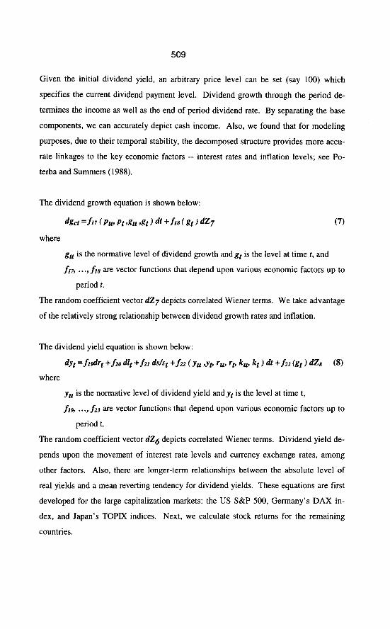
Given the initial dividend yield, an arbitrary price level can be set (say 100) which
specifies the current dividend payment level. Dividend growth through the period de-
termines the income as well as the end of period dividend rate. By separating the base
components, we can accurately depict cash income. Also, we found that for modeling
purposes, due to their temporal stability, the decomposed structure provides more accu-
rate linkages to the key economic factors -- interest rates and inflation levels; see Po-
terba and Summers (1988).
The dividend growth equation is shown below:
d&t =fu C pw pt ,g, ,st ) dt +.fis t gt J dZ7
where
(7)
g, is the normative level of dividend growth and gf is the level at time t, and
fin . . . . fi,J are vector functions that depend upon various economic factors up to
period t.
The random coefficient vector dZ7 depicts correlated Wiener terms. We take advantage
of the relatively strong relationship between dividend growth rates and inflation.
The dividend yield equation is shown below:
dyt =fi&t +fiodlt +h ds/st +fz (yu ,yb rw rb k, kt) dt +fiJkt) d& (8)
where
yu is the normative level of dividend yield andyt is the level at time t,
flh **-, f& are vector functions that depend upon various economic factors up to
period t.
The random coefficient vector dZ6 depicts correlated Wiener terms. Dividend yield de-
pends upon the movement of interest rate levels and currency exchange rates, among
other factors. Also, there are longer-term relationships between the absolute level of
real yields and a mean reverting tendency for dividend yields. These equations are first
developed for the large capitalization markets: the US S&P 500, Germany’s DAX in-
dex, and Japan’s TOPIX indices. Next, we calculate stock returns for the remaining
countries.

510
2.6 Asset Class Construction
The cascade structure provides a framework for building generic asset classes. The fun-
damental asset classes are already defined: cash, government bonds and large capitalized
equities. Other fixed income assets are modeled via the appropriate spreads over gov-
ernment rates. CAP:Link addresses spreads and the underlying interest relationships of
a given fixed income security. This approach extents to real return (or index linked)
bonds based on the real yield curves. Given this methodology, we can calculate foreign
asset returns by combining the foreign country local return with the currency exchange
rate to calculate a total return in the currency of choice.
In addition, we model a number of asset classes outside the fundamental group. Promi-
nent examples include: real estate; venture capital; alternative equity market segments
such as small capitalization stocks; emerging market investments; catastrophe related
securities; and derivatives. CAP:Link addresses these asset classes by providing tools to
describe levels of volatility, serial correlation, relationships to interest rates and infla-
tion, correlations to other asset classes, and relative return expectations. The tools rep-
resent our view of the dominant characteristics important to ALM -- that is, interest rate
and inflation relationships, diversification potential over different time horizons, and
range of potential tradeoffs of risk and expected rewards.
2.7 Alternative Approaches
The classic alternative to stochastic differential equations underlying CAP:Link is the
mean-covariance model. This model assumes either normal or lognormal time inde-
pendent distributions. The user specifies expected values and variances of each asset
category as well as covariances for all pairs of assets. The approach often appears in fi-
nance textbooks and software packages but suffers in realism for ALM since it avoids
features such as mean reversion in interest rates. A second alternative is vector autore-
gressive (VAR). This approach forms a rolling regression analysis in which the inde-
pendent variables -- interest rates, inflation, asset returns, and liability returns in previ-

511
ous periods -- determine the next period values for the economic variables as well as the
asset returns and liabilities. Because of the unstructured nature of the process, VAR has
considerable adaptability to changing economic conditions. It has been employed in
Cariiio et al. (1994) and others. The approach has proven effective for prediction and
pricing applications. At times, however, VAR may produce divergent results for long-
term risk analysis. In order to overcome this problem, VAR can be coupled with equi-
librium conditions as discussed by Boender (1995). A third alternative has been devel-
oped by Wilkie (1995). The approach possesses a cascade structure similar to
CAP:Link. However, there are substantial differences in the form of the equations, in
the calibration process, and in the ordering of the variables in the cascade.
3.0 Implementation Details
Setting the parameters for the stochastic differential equations (1) through (8) presents a
formidable task with conflicting objectives. We separate the process into two steps. In
the first, called assumption setting, we determine the expected level of returns for asset
classes and economic variables. The second, called calibration, calculates the parame-
ter coefficients for the relationship and distribution characteristics, such as correlations,
standard deviations, ranges, rates of convergence, spreads, and other statistics.
3.1 Assumption Setting
For our discussion, assumption setting refers to coefficients that affect risk premiums
and expected rewards. Towers Perrin assesses a return premium appropriate to each
element of risk. The first block focuses on inflation. The second determines the ex-
pected return on cash net of inflation. The third encompasses the spread of long term
interest rates over short term interest rates. Next, corporate bonds require a spread for
quality risk. Large cap stocks assess a spread of expected equity returns over a bond
universe fund. Capital market line relationships (comparing expected return to volatil-
ity) are considered for consistency. This approach depends upon the assumption that
each element of expected return should be appropriate to compensate for a risky char-
acteristic. Determining the relative premiums is based on dissecting the historical re-

512
turns into expectation elements (such as the initial level of interest rates) and valuation
change elements (such as capital gains/losses due to changes in interest rates). An addi-
tional component relates initial condition values to normative assumptions.
Assumption setting is an iterative process: examining the reasonableness of the inputs
and the results, analyzing the sensitivity of the recommendations, and modifying the pa-
rameters until the patterns are deemed acceptable by the economic staff.
3.2 Calibration Procedure
Calibration describes the elements relating to risks characteristics, such as distributional
spreads. This step presents a more challenging technical task than assumption setting.
Target values are determined for identified important relationship and distributional
characteristics of the model based on an analysis of historical values and expert judg-
ment. Calibration parameters are adjusted until the simulated statistics become suffi-
ciently close to the target values. Performing this task uncovers new characteristics.
Non-convex optimization tools can automate the calibration procedure (Mulvey, Rosen-
baum and Shetty 1996), but in the end judgment is required to accept a satisfactory out-
come or demand further investigation of a perplexing element.
3.3 Sampling Procedures
The stochastic differential equations (1) through (8) form the basis for generating sce-
narios - the main CAP:Link output. We employ a sampling procedure based on variance
reduction methods. For example, we have found antithetic variates to be effective for
many applications. Each scenario depicts a single realization of the stochastic equa-
tions, by sampling from the white noise terms, over the planning horizon. The number
of scenarios depends upon the targeted application and the risk aversion of the investor.
For example, a long-term planning horizon coupled with dynamic investment strategies,
such as portfolio insurance, necessitates a relatively large set of scenarios to provide ac-
curate estimates of risks. On the other hand, stable investment strategies, such as dy-

513
namically balanced, involve small market impact costs under volatile conditions and
therefore require fewer scenarios to produce acceptable risk estimates.
3.4 Precision Tests
A critical issue involves reliability of the model’s recommendations, especially relating
to risks and rewards. Accordingly, we conduct stress tests of the proposed strategies by
means of out-of-sample analyses. First, we generate a new set of scenarios based on
further sampling as described in the previous section, or by modifying the parameters of
the stochastic equations and re-generating the results. The precision of the risk meas-
ures and valid confidence limits are estimated by simulating the investment/liability
strategies with the new data. The second risk estimates are compared with the original.
If the two values are close, we deem the precision tests to be a success. Otherwise, we
can employ a larger set for the optimization stage of ALM system.
By employing precision tests, we have found that 500 scenarios is adequate for many fi-
nancial planning purposes. The number of scenarios will need to be substantially in-
creased, however, when the investor displays extreme risk averse.
4.0 Illustration of Pension Planning
Consider the case of a defined benefit pension plan in the US -- the NEWCO company
- which is in the process of developing an investment strategy for its portfolio mangers.
We will discuss the planning process and demonstrate sample forms of analysis. The
approach applies to other long term financial investment decisions (insurance compa-
nies, endowment funds, personal financial planning) with differing emphases (such as
funding decisions).
The process consists of three stages. First, we determine the objectives for the pension
plan and carry out the assumption setting tasks. In the second, we analyzes risks and
rewards for alternative investment strategies. The final stage involves decision making
and implementing the asset and liability allocation strategy. In practice, the process of-

514
ten entails a cycle -- observations made from the analysis lead to modifications in the
objectives and assumptions. The goal is to understand the financial dynamics, not to run
the data through a standardized process and produce a single “answer”.
Assumption Risk and Reward Decision Setting Analysis ’ Making
Figure 3: The three stages for pension planning. The process entails a combination of feedback and revi- sion in order to become comfortable with the recommendations.
Stage 1 : Objective and Assumption Setting
Setting goals for a defined benefit pension plan is often difficult due to the presence of
multiple parties possessing differing interests: beneficiaries, with benefit security or
even benefit enhancement; and plan sponsors, with cost levels and volatility. Taken
from the sponsors’ view, there are alternative bases on which to measure cost: contribu-
tions, expense levels for accounting, long term economic cost, impact on corporate in-
come statement, etc. Differing actuarial bases are possible. Issues of time frame (I
year, 3 years, or longer) and risk measurements (standard deviation, volatility, or
chances of failing to meet some minimum acceptable target) add complexity. To ap-
proach the problem, we focus on the major objectives and stakeholders. Having made a
list of these items, we render projections in order to identify areas of concern. For our
illustration, we examine projections of contributions and timings, funded ratio levels,
and pension expense under current funding and investment policy.
Generating estimates of the future viability and surplus of the pension plan requires four
elements: the scenario generation program; a package for projecting the liability cash-
flows based on the plan’s actuarial rules”; a multi-period investment and contribution
management system (possibly with an optimization component)“‘; and a system for cal-
culating financial and accounting statistics. The four components must fit together with
regard to structure and dependence on key assumptions.

515
We apply the Towers Perrin’s system to assist NEWCO. The resulting estimates for the
range of contributions over the next ten years appear in Figure 4. This projection shows
that the likelihood of making contributions in any one of the next ten years is less than
50%. Since contributions are linked temporally, we must examine the distribution of
cumulative contributions through the decade. Because contributions are strongly af-
fected by funding policy, however, these numbers can be difficult to evaluate”. In some
cases, inadequate cash flows increase the importance of the contributions.
Figure 4: Distribution of contributions. The probability of a contribution in any year is less than 50%
The next issue to consider is the company’s expenses. In the US, pension expenses de-
pend upon accounting and other regulatory rules such as FAS 87, which requires plans
to discount their liabilities at a close to market rate. Figure 5 depicts the range of possi-
ble expenses for NEWCO over the next ten years. We see that they are roughly l-2% of
the company’s payroll. However, there is considerable uncertainty, given the range of
investment returns and the company’s contribution policy during the ensuing period. In

516
fact, there is a reasonable chance that expenses will be negative - indicating income to
the firm.
Figure 5: Distribution of expenses as a percentage of payroll. Expenses can become negative in future years indicating income to the firm.
As a consequence of the investment asset mix and the contribution policy, we can ob-
serve the health of the pension plan surplus over the 10 year planning horizon. One
view of the surplus is the Accumulated Benefit Obligation (ABO) - roughly the amount
of money needed to pay off the current promised liabilities at present value. Figure 6
shows the range of possible ABO numbers. Here, the 100% value indicates a fully
funded pension plan on a ABO basis, or there is just enough asset value to compensate
for liabilities at present value (discounting at current government non-callable rates).
Amounts above 100% are in surplus, whereas amounts below 100% indicate a deficit. A
company’s required contribution depends upon the value of the ABO numbers.
Projecting the impact of today’s decisions on a company’s future wealth make sense for
long term investors. A multiyear simulation tool based on discrete scenarios is essen-
tial. To make these projections, we must address the interaction of economic variables
such as interest rates and inflation levels with capital market returns. Also, the individ-

517
ual patterns impact the financial results, such as pension expenses. In addition to the
economic and capital market simulations, as provided by CAP:Link, we must convert
this information into the relevant financial statistics. The calculation ought to be
straightforward, but in practice many regulatory, timing, and other technical issues must
be addressed. All financial projections presented have been produced by Towers Per-
rin’s FIN:Link system.
ABO Funded Ratio at end 01 Five “ears
160
170
160
150
140
E
F 130 $
120
110
100
9c
60
r
+
, --
/
1996 1997 1996 1999 ZOOI 2001 2002 2003 2004 2005
Year
901h%
75th%
50th%
251h%
1 Oth%
Figure 6: Distribution of ABO funded ratios over the next 10 years. The NEWCO pension plan is likely to be in surplus during the period, given the proposed contribution policy.
Contribution, expense, and other projections depend upon calibration assumptions.
Similar to the objective setting process it is useful to examine the projections to access
their reasonableness and also to provide more insight into the drivers behind the finan-
cial projections.

518
For NEWCO, we reflect the economic variables at the beginning of 1996 -- adjusting
the assumptions to an “equilibrium” condition, where long term expectations are set
equal to current conditions and the spread between expected returns of various asset
classes equal the normative assumptions. The normative approach helps develop broad
policy guidelines. Alternatively, the assumptions could equal the company’s best long-
term estimates. This approach is suitable where consideration of strategic shifts in asset
allocation are under review. Of course, consideration should be given to whether fund
managers will be capable of performing ongoing analysis and adjustments to invest-
ments to reflect changing conditions.
Graphs showing the projections of inflation and interest rates (Figures 7, 8, and 9) -- the
primary liability drivers -- are presented below along with the range of returns for each
of the asset classes.
U.S. PdCC inm,,.¶n ,Compo”nd,
Figure 7: Distribution of estimated price inflation in US. These ranges reflect historical inflation in the US over the past 40 years.

Figure 8: Distribution of estimated US T-bond yields. These results assume that long term interest rates equal the starting interest rates (I January 1996 in this case).
Figure 9: Distribution of ten year compounded returns. Cash becomes dominated by both stock and bond indices as the horizon lengthens.

520
After completing this step, we pinpoint a specific concern -- funded levels falling below
the 90% ratio of assets to the present value of liabilities. In an actual assignment, sev-
eral elements for further investigation emerge. For example, the time horizon is signifi-
cant. It is appropriate to investigate both the immediate term (l-3 years) and the longer
term (5+ years). The former is critical - due to the nature of evaluating management
performance by stockholders and other stakeholders. The long term must be considered
as well: pension plan sponsors have a fiduciary responsibility to see that the company’s
promised benefits will be realized. Again a real world case would involve multiple time
horizons, perhaps with differing objective elements: a short time horizon for funded
status, and a longer one for pension expense levels. In this illustration, we focus on a
five year time horizon.
Stage 2 : Analysis of Risks and Rewards
Efficient frontiers can be developed at various time horizons. Traditional efficient fron-
tiers plot expected investment return versus the volatility of asset return over a single
period - an asset only concept; see Konno et al. (1993) and Kroll et al. (1984). It is use-
ful to understand the recommendations of the “standard single period asset only ap-
proach” so that they can be compared with a comprehensive ALM approach. To address
standard practice, we calculate an asset-only frontier with a five year time horizon
(Figure 10). Additional efficient frontiers should reflect differing elements of the ob-
jectives identified in Stage 1. Thus, we select average funded ratio at the end of five
years as the reward measure and first-order downside risk with a 90% target as the risk
measure (Figure 11). First-order downside risk equals the average shortfall below the
target averaged over all scenarios (including those where there is no shortfall). For ref-
erence, second-order downside risk equals the average squared shortfall. First-order
downside risk breaks into the product of two intuitive risk measures: the probability of
shortfall and the average shortfall when one exists.
The scope of a risk analysis can be portrayed on a risk ladder (Mulvey 1996) with five
rungs: 1) total integrative risk management; 2) dynamic asset-liability; 3) static asset-
liability; 4) static asset only (a.k.a. Markowitz mean variance portfolios); and 5) single

521
security risks. Most current risk analyses are conducted at rungs 3 or 4. However, there
are several groups that are pushing the analysis to higher, more comprehensive levels on
the risk ladder. In this context, there are several criteria for measuring risk, including
variance for symmetric outcomes, semi-variance and downside risks for asymmetric
outcomes, and von Neumann Morganstern expected utilities. Ultimately, an organiza-
tion ought to be concerned with risks to its net worth - at the top of the risk ladder.
Illustration E tflclent Frontier Asset E tliclent F rontler 5 Year TImI HOrlzOn
II
Figure 10: An asset-only efficient frontier. Cash and bonds are considered the more conservative category for short term investors without liabilities.
We might consider several efficient frontier calculations with a variety of risk and re-
ward measures, some which might be a weighted combination of differing measures.
The goal is to find a set of candidate portfolios based on the efficient frontiers which
might best meet the competing considerations. In theory, this step could be done by
constructing the “correct” risk and reward measures and performing the efficient frontier
calculation on these objectives. In practice, however, the correct measures become

522
known as the analysis progresses. Employing candidate portfolios help draw out this
knowledge. In this illustration we limit the discussion to the two frontiers described
above. Calculating efficient frontiers over multiple time periods requires non-linear sto-
chastic optimization programs; see Mulvey, Armstrong and Rothberg (1995)‘. Addi-
tionally, because of the non convexity due to the dynamic aspects of multi-period ALM
and the lack of performance guarantees, the investor must be careful to access if a global
optimal solution has been found. This consideration argues for the candidate portfolio
approach. Based on this analysis, we focus on promising areas on the frontiers. For
comparison, portfolios recommended by the asset-only efficient frontier have been
plotted on the funded ratio efficient frontier. Differences are quite dramatic -- the low-
risk portfolios from the asset-only efficient frontier are highly risky from a funded ratio
perspective at the five year point” (see Figure 11).
Illustration E fflclent F rontlor AB 0 S urptur E tflclenl F rontler 5 veal TlnlO Horlron
,25~.................................,o -.-.- -.....
Figure 11: An alternative efficient frontier with downside ABO risk. Treasury bonds are considered the least risky asset based on the investor’s liability structure.

523
By selecting portfolios from the most attractive regions of the efficient frontiers we de-
velop a list of candidate portfolios. NEWCO’s efficient frontier in Figure I1 suggests
substantial investments in small capitalization and international stocks and real estate.
In practice, these recommendation might be limited for liquidity and prudence issues.
Constraints on the optimization could be readily applied and the optimization re-run to
generate a revised investment strategy.
Stage 3 : Decision Making and Implementation
We have chosen two candidate portfolios for comparing the distributions of contribu-
tions, expense, and funded ratio. In addition, it is useful to consider the differences in
potential performance relative to NEWCO’s current position. For alternatives 1 and 2,
contributions and expenses are reduced, both on absolute range and as relative im-
provements over the current allocation (Figures 12 and 13). In this case, we see that al-
though the first alternative has the potential for higher absolute levels of expense, the
distribution of improvement from the current portfolio is much more attractive than for
the second. Alternative I outperforms the current policy approximately 70% of the
time, while alternative 2 outperforms the current policy about 50% of the time (Figure
14). From this perspective, alternative I appears superior to the current policy as well as
alternative 2. Similarly, alternative 1 has the highest ABO funding ratio on average
(Figure 15).
Figure 12: Distribution of contribution over 5 years. Both alternative I and 2 reduce contribution over the 5 years.
524
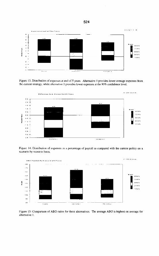
Figure 13: Distribution of expenses at end of 5 years. Alternative I provides lower average expenses from the current strategy, while alternative 2 provides lower expenses at the 90% confidence level.
I I
2 0
, I
, 0
D I
0 .a
.,,,, I .,,..
t
Figure 14: Distribution of expenses as a percentage of payroll as compared with the current policy on a scenario by scenario basis.
Figure IS: Comparison of ABO ratios for three alternatives. The average ABO is highest on average for alternative I.

525
Once an allocation strategy is found, it is essential to carry out a sensitivity analysis. If a
higher allocation to equity is suggested over the current asset allocation, for example,
we recommend that the investor employ assumptions which reduce this spread. This ap-
proach applies to all asset classes targeted for increase in allocation. Observations made
at this stage may lead back to an earlier stage. Simulation lends itself to pinpointing the
cause of a particular result. Recommendations can be segmented by inflation, interest
rates, equity returns, contribution levels, or other proposed causes. The analysis leads to
an improved understanding of the investment dynamics. Combining this with other
factors, such as liquidity, perceptions, transition problems, and implementation capabil-
ity produce a decision.
The analysis may also suggest modifying the pension plan design, contribution policy,
or asset and liability smoothing in order to improve overall financial performance. In
addition, long term ALM systems can address more focused questions, such as whether
and how much currency hedging is appropriate, how unexpected inflation would effect
the contributions and other measurements, and how short-term funding decisions will
impact longer-term risks.
5.0 Conclusions and Future Directions
Towers Perrin’s system provides an internally consistent approach for generating capital
market scenarios over long-term horizons. It captures an extensive range of market re-
lationships -- making it an effective tool for risk analysis. There are several directions
for future research. First, the system easily extents for new asset categories. For exam-
ple, combining the purchase of equity and selling an off-setting call option -- buy-
writing -- can be modeled as a separate asset category. This strategy is effective in
volatile and driftless markets. The options can be valued in the usual manner via arbi-
trage free approaches since the risk free rates, volatility and other factors are known
within a scenario. Buy-writing may be attractive for risk averse investors since down-
side risks are considerably reduced over a pure equity category. Another promising as-
set category involves securitizing catastrophic (CAT) insurance, as implemented by the
526
Chicago Board of Trade. Here, risks are uncorrelated with the returns of other asset
categories. Investigating the pros and cons of these and other asset categories is made
possible due to the system’s flexibility.
Another extension is to employ the currency exchange rates for hedging strategies. Re-
member that local returns for countries outside the home country are inaccessible due to
uncertain currency movements and the lack of equilibrium with respect to implied for-
ward rates (Brinson 1993). Since the system defines currency as a separate economic
factor, we can evaluate cross hedging strategies. See Sorensen (1993) for an example
application. Next, we can assist corporations in setting organizational goals. For in-
stance, we could evaluate alternative contribution policies. By analyzing policies under
stressful conditions such as a recession, we can pinpoint total risks - rather than sub-
optimizing the risks for individual components - such as portfolios in a single country.
In conclusion, multi-stage financial models cannot replace an understanding of capital
markets. Rather, they aid in analyzing the competing issues of risks and rewards over
time. As such, the capital market projections must provide a representative range of
plausible scenarios. The global CAP:Link provides this information in a practical and
internally consistent fashion.
References
Amin, K. I. and R. A. Jarrow, “Pricing Foreign Currency Options Under Stochastic In-
terest Rates,” Journal of International Money and Finance, 10, 1991, 3 10-329.
Berger, A. J. and J. M. Mulvey, “Integrative Risk Management for Individual Inves-
tors,” in World Wide Asset and Liability Modeling, (eds., W.T. Ziemba and J. M.
Mulvey), Cambridge University Press, 1996.
Black, F. and R. Litterman, “Global Portfolio Optimization,” Financial Analysts Jour-
nal, September-October 1992,28-43.
Boender, G. C. E., “A Hybrid Simulation/Optimization Scenario Model for As-
set/Liability Management,” Report 95 13/A, Erasmus University, Rotterdam,
1995.
527
Boothe, P. and D. Glassman, “The Statistical Distribution of Exchange Rates,” Journal
of International Economics 22, 1987,297-3 19.
Brennan, M.J. and ES. Schwartz, “An Equilibrium Model of Bond Pricing and a Test of
Market Efficiency,” Journal of Financial and Quantitative Analysis,” 17, 75-
100, March 1982.
Brinson, G. P., “You Can’t Access Local-Currency Returns,” Financial Analysts Jour-
nal, May-June 1993, IO.
Cariiio, D.R., T. Kent, D.H. Myers, C. Stacy, M. Sylvanus, A. Turner, K. Watanabe and
W. T. Ziemba, “The Russell-Yasuda Kasai Model: An Asset Liability Model for
a Japanese Insurance Company using Multi-stage Stochastic Programming,” In-
te$aces, 24, Jan-Feb 1994,29-49.
Choie, K. S., “Currency Exchange Rate Forecast and Interest Rate Differential,” The
Journal of Portfolio Management, Winter 1993,58-64.
Cochran, S. J. and R. H. DeFina, “Predictable Components on Exchange Rates,” The
Quarterly Review of Economics and Finance,” Vol. 35, No. 1, Spring 1995, l-
14.
Dempster, M., “The Development of the Midas Debt Management System,” in World
Wide Asset and Liability Modeling, (eds., W.T. Ziemba and J. M. Mulvey),
Cambridge University Press, 1996.
Hogan, M., “Problems in Certain Two-Factor Term Structure Models”, The Annuls of
Applied Probability, 3, 1993, 576-581.
Huber, P., “A Review of Wilkie’s Stochastic Model,” Actuarial Research Paper No. 70,
The City University, London, 1995.
Konno, H., S. Pliska and K. Suzuki, “Optimal Portfolio with Asymptotic Criteria”, An-
nals of Operations Research, 45, 1993, 187-204.
Kritzman, Mark, “What Practitioners Need to Know About Currencies,” Financial
Analysts Journal, March-April 1992,27-30.
Kritzman, Mark, “The Optimal Currency Hedging Policy with Biased Forward Rates,”
The Journal of Portfolio Management, Summer 1993,94-100.

Kroll, Y., H. Levy and H. Markowitz, “Mean Variance Versus Direct Utility Maximiza-
tion,” Journal of Finance 39, 1984,47-62.
Lasdon, L., A. Warren, A. Jain, and M. Ratner , “Design and Testing of a GRG Code for
Nonlinear Optimization,” ACM Transacfion on Mafhemafical Sojtware, 4, 1978,
34-50.
Mahieu, R. and P. Schotman, “Neglected Common Factors in Exchange Rate Volatil-
ity,” J. of Empirical Finance, 1, 1994,279-3 11.
Mulvey, J. M., J. Armstrong and E. Rothberg, “Total Integrative Risk Management,”
Risk Magazine, June 1995.
Mulvey, J. M., “It Always Pays to Look Ahead,” Balance Sheet, Vol. 4, No. 4, Winter
1995/96,23-27.
Mulvey, J. M., “Integrating Assets and Liabilities for Large Financial Organizations,” in
W. W. Cooper and A. B. Whinston, Eds., New Directions in Computational
Economics, Kluwer Academic Publishers, 1994, 135 150.
Mulvey, J. and W. Ziemba, “Asset and Liability Allocation in a Global Environment,”
in Finance, R. Jarrow et al., Eds., Handbooks in Operations Research and
Management Science, Vol. 9, North Holland, 1995,435-463.
Perold, A.F., and W.F. Sharpe, “Dynamic Strategies for Asset Allocation,” Financial
Analysts Journal, 16-27, Jan. 1988.
Poterba, J. M. and L. H. Summers, “Mean Reversion in Stock Prices: Evidence and Im-
plications,” Journal of Financial Economics, 22,27-59, Oct. 1988.
Sorensen, E., Mezrich, and D. Thadani, “Currency Hedging through Portfolio Optimi-
zation,” J. of Portfolio Management, Spring, 78-85, 1993.
Wilkie, A. D., “More on a Stochastic Asset Model for Actuarial Use,” Institute of Actu-
aries and Faculty of Actuaries, 1995.
i The US government will begin selling index linked bonds in late 1996. Thus, estimates of inflationary expectations will be available as a traded security.
ff,Towers Penin’s system is called VALCAST. ]II Towers Perrin’s system, OwLink, is based on Leon Lasdon’s GRG package (1978). I” Contribution in the US is based on a complex set of regulatory rules and employee preferences. “Towers Perrin’s 0PT:Link system solved these efficient frontier calculations. Vi We have discovered numerous similar situations in practice.


![USA 2009 200907 2009 Towers Perrin-IsR Safety Culture Brochure[1]](https://cdn.vdocuments.us/doc/165x107/54680a0fb4af9f3a3f8b5b02/usa-2009-200907-2009-towers-perrin-isr-safety-culture-brochure1.jpg)


