Download - The Physics of Radio.pdf

7/27/2019 The Physics of Radio.pdf
http://slidepdf.com/reader/full/the-physics-of-radiopdf 1/11
The Physics of Radio
By John White
Radio Bands and Channels
The use of wireless devices is heavily regulated throughout the world. Each country has a governmentdepartment responsible for deciding where and how wireless devices can be used, and in what parts of
the radio spectrum. Most countries allocate parts of the spectrum for open use, or “license-free” use.
Other parts of the spectrum can only be used with permission or “license” for each individualapplication.
Most wireless products for short-range industrial and commercial applications use the license-free
areas of the spectrum, to avoid the delay, cost and hassle of obtaining licenses. The license-free bandsare also knows as ISM bands - “Industrial, Scientific & Medical”. In many countries there areseveral ISM bands available, in different
parts of the spectrum.
The radio spectrum is split into frequency
“bands” and each band is split intofrequency “channels”. The width of each
channel is normally regulated. The
channel width dictates how fast data can be transmitted - the wider a channel,
the higher the data rate.
Higher frequency bands are wider, so the
channels in these bands are also wider,allowing higher wireless data rates. For
example, licensed channels in the lower frequencies (150 – 500 MHz) are often regulated to 6.25
or12.5KHz, whereas channels in the license-free 2.4GHz band can be hundreds of times wider.
However lower frequency bands have much longer operating distances. With wireless data, there isalways a trade-off between distance and data rate. As radio frequency increases, the possible data rate
increases, but operating distance decreases.
Fixed Frequency, Narrow-band
Generally, industrial wireless communications uses either fixed frequency radio channels or a spreadspectrum radio band.
“Fixed frequency”, as the name implies, uses a single frequency channel - radios initiate and maintaincommunications on the same frequency at all times. Fixed frequency channels can be licensed-free or
licensed, although the license-free fixed frequency channels in America are seldom used for industrial
applications. A licensed channel is licensed to the operator of the wireless system by a governing bodyin each country, such as the US Federal Communications Commission (FCC). A radio license protects
a channel against other users in a specified geographic area, and also specifies the RF power levels
which may be used. Generally licensed channels allow much higher power levels that license-freechannels.
:
:
INCREASINGFREQUENCY
:
:
::
RADIOBAND
RADIOCHANNEL
CHANNELWIDTH

7/27/2019 The Physics of Radio.pdf
http://slidepdf.com/reader/full/the-physics-of-radiopdf 2/11
Fixed frequency in the context of industrial use have a narrow width, and are often referred to as
“narrow-band” channels.
Spread Spectrum
Spread spectrum radios use multiple channels within a continuous band. The frequency is
automatically changed, or transmissions use multiple frequencies at the same time, to reduce theeffects of interference. While there are several types of spread spectrum techniques, the two most
common are Frequency Hopping Spread Spectrum (FHSS) and Direct Sequence Spread Spectrum
(DSSS) .
Spread spectrum allows a large number of wireless systems to share the same band reliably. Thereliability of fixed frequency channels is dependant on no other system using the same channel at the
same time. Spread spectrum provides a method of interleaving a large number of users into a fixed
number of channels.
Frequency Hopping Spread Spectrum (FHSS) has the frequency of the transmitted message periodically changed (or hopped) . The transmitter hops frequencies according to a pre-set sequence (or
hop sequence). The receiver either stays synchronized with the transmitter hopping, or is able to detect
the frequency of each transmission.
FHSS can hop rapidly, several times per message, or transmit a complete message (or data packet)
and then hop. Each transmitter hops to a particular hop-sequence, which it chooses automatically or isuser-configured. FHSS hopping sequences are pseudo-random, in that the probability of a foreign
transmitter hopping to a particular channel appears to be random.
Direct Sequence Spread Spectrum (DSSS) differs from FHSS in that the transmitted data packet is“spread” across a wide-channel, effectively transmitting on multiple narrow channels simultaneously.
Data packets are modulated with a pseudo-random generated key, normally referred to as a “chipping-
key”, which spreads the transmission across the wide-band channel. The receiver decodes andrecombines the message using the same chipping key to return the data packet to its original state.
Item 2
Being a log scale, doubling signal power adds another 3dB. Increasing four times adds 6dB (2 x 3),
increasing 8 times adds 9dB (3 x 3). Similarly halving a signal removes 3dB. Useful “rules of thumb”are
x 2 = +3dB x 5 = +7dB x 10 = +10dB
x 0.5 = -3dB x 0.2 = -7dB x 0.1 = -10dB
1mW = 0dBm 10mW = 10dBm 50mW = 17dBm
100mW = 20dBm 200mW = 23dBm 1W = 30dBm
Item 3
The Effect on Frame Rates
As well as considering the effect on bit error rate, the effect on “frame error rate”, FER is important.
FER is the rate of corrupted data packets.
Because the instantaneous level of background noise follows a random probability function, any and
every wireless data packet, or frame, is vulnerable to random noise “attack” that can corrupt individual bits. Forward-error-correction (FEC) techniques can be used to recover the corrupted bits however for
messages without FEC, the whole frame becomes corrupt if one bit is corrupted.

7/27/2019 The Physics of Radio.pdf
http://slidepdf.com/reader/full/the-physics-of-radiopdf 3/11
The probability of a corrupted frame from random noise attack increases with its “air-time” - the
overall transmission time of the message. This depends on the length of the message (number of bits)
and the transmitted data rate. The longer the message, the higher the probability of messagecorruption, but the higher the data rate, the probability decreases.
So higher data rate has two effects; increasing BER but reducing FER. The significance of each effect
depends on the average SNR and the volatility of the noise. Where noise is from other transmitters in
the same band, noise level volatility can be very high. Generally there will be an optimum data ratewhich balances these contrary effects. Forward error correction techniques significantly reduce the
effects of random noise attack, however reduces the effective data rate.
Item 4
Section 3 Radio Propagation
How far will a radio signal transmit
reliably? A radio signal is transmitted at acertain signal (power) level, but received
at a much lower level. Radio signals are
attenuated as they pass through air or other media. The amount of signal loss over the
radio path determines how far a radio
signal will travel. When a radio signal falls below the data sensitivity, then it is no
longer received reliably. When the radio
signal falls below the “fade margin”, the
signal becomes marginal.
There are many factors which affects signal power levels and signal attenuation:
RF Power
“If you transmit more radio signal, then the signal will go further” - this is a fairly obvious statement.
It means that if you increase the RF power level at the transmitter, then the power received at the
receiver will increase. But how does this relate to distance?
Radio signals through a constant media attenuate proportionally to the square of distance. That is,
in a clear radio path through air, if you double
the distance, then the received signal level willdecrease to ¼ (or –6dB). Similarly if you halve
the distance, the received signal increases 4
times (or +6dB).
The same relationship exists with transmitter power:
as RF power increases, distance increasesby a square-root effect
d new = d old x √( Pnew / Pold ); where d is distance and P is RF power
To double reliable distance, you need to increase power level four times - i.e. you need to increase
power by 6dB. Or if you halve power levels, the distance will decrease to approx 70% (1/√2).
Receiver Sensitivity
Better receiver sensitivity means that a receiver can demodulate data at lower signal levels - or that a
signal can be attenuated further. Devices with better receiver sensitivity can achieve longer distances.
Distance
RF Power
Power inWatts
Power indB
Distance
RF Power (dBm) alonga radio path
Transmitter
Min. signal level for
reliable operation

7/27/2019 The Physics of Radio.pdf
http://slidepdf.com/reader/full/the-physics-of-radiopdf 4/11
Improving receiver sensitivity has the same effect as increasing transmitter power. Improving receiver
sensitivity by 1dB can increase distance up to 12%.
Frequency
As radio frequency increases, the amount of
attenuation increases in the same way asdistance - that is, signal attenuation increases
with the square of frequency. Over the same
radio path, as the frequency increases, theradio signal decreases by a square relationship
- if the frequency doubles, the signal drops to
¼ etc.
As distance is also related to the square of radiosignal, then the relationship between frequency and distance is inversely proportional –
as frequency increases, reliable distance decreases proportionally
d new = d old x ( f old / f new ); where d is distance and f is frequency
This is only an approximate relationship as many other factors come into play.
Nature of the radio path.
Obstructions in a radio path have a major effect on the expected reliable distance.
The frequencies used for industrial wireless products is often called “line-of-sight” frequencies. But
this doesn’t mean that line-of-sight is required for reliable operation. “Line-of-sight” means that the
transmitted radio signal will radiate in straight lines, instead of curving around the earth’s curvature.
Radio signals will pass through some obstacles (for example, buildings) and will also reflect fromsome surfaces (for example, metal tanks/vessels, rock cliffs). Radio signals won’t pass through
obstacles like hills, however some of the radio signal can diffract (bend) around this type of obstacle.
The general rule is that obstacles decrease the reliable operating distance.
Most wireless products are specified with a “line-of-sight distance” - this is the distance that can beexpected to be achieved with no obstacles in the radio path. The curvature of the earth is an obstacle,
so in most cases these distances can be only achieved by elevating the antennas above ground level.At normal eye level across a flat plain, the distance to the horizon is 5.5 km (3 miles) however this
increases to over 20 km (13 miles) if you are 30 meters (100 feet) above the ground.
Generally, transmission distances will increase if you increase the height of antennas.
Typical line-of-sight distances (miles) 10dB fade margin
2.4 GHz 36dBm / 4W ERP WiFi 3
2.4 GHz 36dBm / 4W ERP FHSS 6
915 MHz 36dBm / 4W ERP FHSS 15
915 MHz 12dBm / 15mW ERP FHSS 1
450 MHz 40dBm / 10W ERP Narrow band 25
Some “rules of thumb” are:
• Distances more than half of the rated “line-of-sight” range cannot tolerate any obstacles in theradio path - you need to establish a true line-of-sight path for reliable operation.
• Distances within 10 – 50% of rated “line-of-sight” range can tolerate some obstacles.
Distance
Frequency

7/27/2019 The Physics of Radio.pdf
http://slidepdf.com/reader/full/the-physics-of-radiopdf 5/11
Radio path pattern between two antennas
• Distances less than 10% can tolerate a lot of obstacles.
• Obstacles have more of a blocking effect if they are close to one end of the radio path. The overallradio signal spreads out - the dispersion pattern between two antennas looks like an Americanfootball.
• Beware of trees. Although individual trees do not posemuch of an obstacle to a radio signal, a group of trees
do. Radio signals do not penetrate far into forests or
woods. Performance varied depending on season (noleaves or lots of leaves) and weather (wet leaves vs dry
leaves).
Heavily congested radio paths found on industrial sites and
factories can still be reliable because the distances are short. The radio path is made up of manyseparate paths, some penetrating obstacles, some reflecting from other obstacles. Most products in
industrial applications use the license-free ISM bands, and distance performance varies considerably
due to the differing frequency/power characteristics of the different ISM bands.
It is possible to estimate the reliability of radio paths using software packages, however the result can be misleading because of obstacles that the package is not aware of. The only accurate way of
knowing if a radio path will be reliable is to test. For short distance paths, this can be done easily and
quickly. But for long distance paths, testing can be difficult and take a long time to perform.
Antennas
Antennas are carefully designed for a particular frequency to radiate and receive the radio signal.Without antennas very little of the RF energy generated by the wireless device will be radiated.
Antennas can be mounted directly to the wireless unit, or mounted separately and connected to the
device by coaxial cable. The coaxial cable attenuates the RF signal in the same way as transmitting
through air or other media - so there is a signal loss in the cable.
Antennas can be designed to focus the RF energy in certain directions, in the same way that a lens and
parabolic mirror focuses light in a flashlight. In the designed directions, the RF energy is magnified
with a specific gain (normally expressed in dB). The gain can be high, with gains of 5 to 10dB (or 7to10 times magnification) fairly normal.
The gain of an antenna can be used to compensate for loss in a coaxial cable, and to also increase the
effective power radiated from the transmitting antenna. In the same way, antennas magnify the signal
received at the receiving antenna.
So high gain antennas have the sameeffect as increasing RF power at the
transmitter, and improving receiver
sensitivity at the receiver, both of which
increase reliable distance.
Selecting the right antenna for a particular radio path is important, and can make the
difference between reliable operation and
poor operation.
Antenna Basics
Antennas are designed and built to suit a particular frequency or frequency band. If you use an
antennas designed for a different frequency, then it will only radiate a small portion of the generated
RF power from the transmitter, and it will only absorb a small portion of the RF signal power for thereceiver. Using the correct frequency antenna is very important.
Distance
RF Power (dBm) alonga radio path Transmitter
Min. signal level for reliable operation
Using a higher gainantenna

7/27/2019 The Physics of Radio.pdf
http://slidepdf.com/reader/full/the-physics-of-radiopdf 6/11
Antennas are compared to a theoretical isotropic antenna. This antenna
radiates all of the power from the transmitter in a 3-dimensional
spherical pattern - very much like a point source of light without anymirrored reflectors.
An isotropic antenna is theoretical only because in the construction of
antennas, the radiation pattern becomes distorted in certain directions.
A “dipole” antenna is manufactured with an active “radiator” with a
length equal to ½ the wavelength of the design frequency.
The RF power envelope radiated by a dipole is distorted by radiating more power in the horizontal plane and less in the vertical plane - that is, there is more power radiated to the sides than up and
down.
The effective RF power to the sides has increased, and the effective power up/down has decreased.
The term “effective radiated power” or ERP is used to measure the power radiated in specificdirections. The difference between the effective
radiated power and the transmitter power is called
the “antenna gain”, and is normally expressed in
dB.
Antenna Gain = P ERP / PTX
The gain of a dipole antennas to the sides of the
antenna is + 2.14 dB. This means the effectiveradiated power to the sides of the antenna is 2.14dB
more than the power from the transmitter. The gain in the up/down direction will be negative,
meaning that the effective radiated power in these directions is less than the power from the
transmitter.
A dipole mounted vertically has positive
gain in the horizontal plane - this is calledvertically polarized. If the antenna is
mounted horizontally, then the power will
radiate from the sides of the dipole, butnot from the ends - this radiation is
horizontal polarity.
The radiation pattern can be distorted further by connecting multiple dipole elements together. Theseantennas, known as “collinears”, have a higher gain to the sides and a more negative gain up/down.
Collinear antennas are normally manufactured with gains of 5dB, 8dB or 10dB compared to thetransmitter power. When antenna gains are expressed as a comparison to the transmitter power, it is
called “isotropic gain”, or gain compared to an isotropic antenna. Isotropic gains are expressed as“dBi”. Another common way to express gain is “as compared to a dipole” - these gains are expressed
as “dBd”. The difference between dBd and dBi is the intrinsic gain of a dipole, 2.14dB (normallyrounded to 2dB).
dBd = dBi - 2
Dipole and collinear antennas are called omni-directional as they transmit equally is all directions inthe horizontal plane. Directional antennas distort the radiation patterns further and have higher gains
in a “forward” direction.
RADIATION PATTERN FOR DIPOLE ANTENNAWITH VERTICAL POLARITY
RADIATION PATTERN FOR COLLINEAR ANTENNA
RADIATION PATTERN FORISOTROPIC ANTENNA
7/27/2019 The Physics of Radio.pdf
http://slidepdf.com/reader/full/the-physics-of-radiopdf 7/11
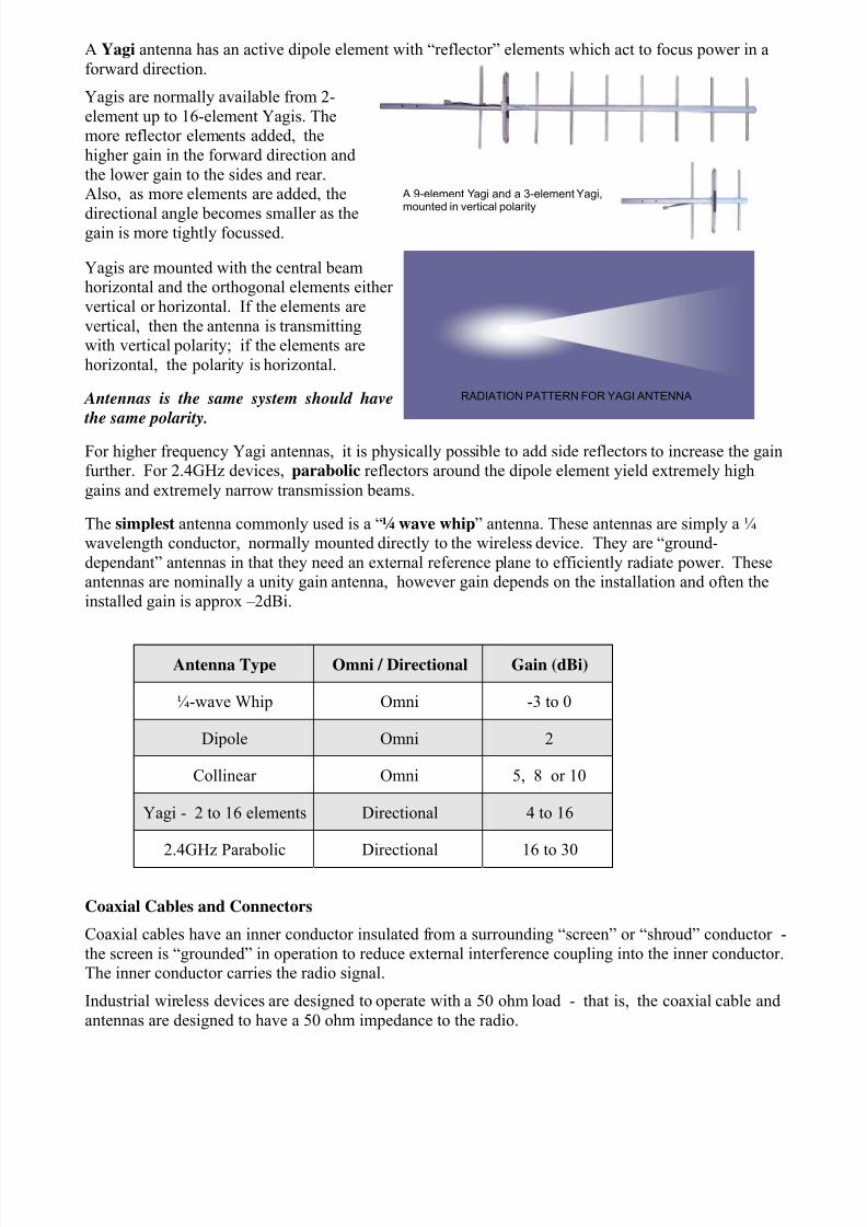
A Yagi antenna has an active dipole element with “reflector” elements which act to focus power in a
forward direction.
Yagis are normally available from 2-
element up to 16-element Yagis. Themore reflector elements added, the
higher gain in the forward direction and
the lower gain to the sides and rear.Also, as more elements are added, the
directional angle becomes smaller as thegain is more tightly focussed.
Yagis are mounted with the central beamhorizontal and the orthogonal elements either
vertical or horizontal. If the elements are
vertical, then the antenna is transmittingwith vertical polarity; if the elements are
horizontal, the polarity is horizontal.
Antennas is the same system should have
the same polarity.
For higher frequency Yagi antennas, it is physically possible to add side reflectors to increase the gainfurther. For 2.4GHz devices, parabolic reflectors around the dipole element yield extremely high
gains and extremely narrow transmission beams.
The simplest antenna commonly used is a “¼ wave whip” antenna. These antennas are simply a ¼wavelength conductor, normally mounted directly to the wireless device. They are “ground-
dependant” antennas in that they need an external reference plane to efficiently radiate power. Theseantennas are nominally a unity gain antenna, however gain depends on the installation and often the
installed gain is approx –2dBi.
Antenna Type Omni / Directional Gain (dBi)
¼-wave Whip Omni -3 to 0
Dipole Omni 2
Collinear Omni 5, 8 or 10
Yagi - 2 to 16 elements Directional 4 to 16
2.4GHz Parabolic Directional 16 to 30
Coaxial Cables and Connectors
Coaxial cables have an inner conductor insulated from a surrounding “screen” or “shroud” conductor -
the screen is “grounded” in operation to reduce external interference coupling into the inner conductor.The inner conductor carries the radio signal.
Industrial wireless devices are designed to operate with a 50 ohm load - that is, the coaxial cable and
antennas are designed to have a 50 ohm impedance to the radio.
A 9-element Yagi and a 3-element Yagi,mounted in vertical polarity
RADIATION PATTERN FOR YAGI ANTENNA
7/27/2019 The Physics of Radio.pdf
http://slidepdf.com/reader/full/the-physics-of-radiopdf 8/11
At the high frequencies used in wireless, all insulation appears capacitive, and there is loss of RF
signal between the inner conductor and the screen. The quality of the insulation, the frequency of the
RF signal and the length of the cable dictates the amount of loss. Generally, the smaller the outer diameter of the cable, the higher the loss; and loss increases as frequency increases. Cable loss is
normally measured in dB per distance - for example, 3 dB per 10 meters, or 10db per 100 feet.
The following table shows the losses of typical types of coaxial cables.
Loss (dB per 30 m)Coaxial cable Outer diameter(mm) 450MHz 900 MHz 2.4GHz
RG58C/U 5 13.5 18.2
RG58 Cellfoil 5 6.9 9.0 16.5
RG213 10 5.0 7.4 14.5
LDF4-50 16 1.6 2.2 3.7
Cables need special coaxial connectors fitted. Generally connectors have a loss of 0.1 to 0.2 dB per connector.
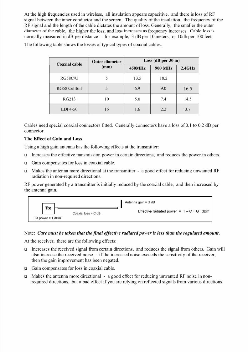
The Effect of Gain and Loss
Using a high gain antenna has the following effects at the transmitter:
Increases the effective transmission power in certain directions, and reduces the power in others.
Gain compensates for loss in coaxial cable.
Makes the antenna more directional at the transmitter - a good effect for reducing unwanted RFradiation in non-required directions.
RF power generated by a transmitter is initially reduced by the coaxial cable, and then increased bythe antenna gain.
Note: Care must be taken that the final effective radiated power is less than the regulated amount.
At the receiver, there are the following effects:
Increases the received signal from certain directions, and reduces the signal from others. Gain will
also increase the received noise - if the increased noise exceeds the sensitivity of the receiver,
then the gain improvement has been negated.
Gain compensates for loss in coaxial cable.
Makes the antenna more directional - a good effect for reducing unwanted RF noise in non-
required directions, but a bad effect if you are relying on reflected signals from various directions.
TxTX power = T dBm
Coaxial loss = C dB
Antenna gain = G dB
Effective radiated power = T – C + G dBm

7/27/2019 The Physics of Radio.pdf
http://slidepdf.com/reader/full/the-physics-of-radiopdf 9/11
Item 5
It is up to wireless device designers and system integrators to use wireless products which arespectrally efficient - that is, devices which minimize transmission traffic within the requirements of
each individual application.
For example, consider a wireless unit transmitting the level of a storage tank 50 times every second. If the application only requires a level accuracy of 0.5%, and at maximum process conditions, the level
cannot physically change by 0.5% in less than one minute, then there are a lot of excess wireless
transmissions. These unnecessary transmissions contribute to the overall radio interference, not onlywithin the same plant or factory, but also in the plants and factories surrounding the tank-farm.
Devices with more sophisticated communications control will reduce this level of interference. If the
wireless unit was configured to only transmit once every minute, then the excess communications
would be reduced significantly. Even better, if the wireless unit only transmitted on a 0.5% change inlevel (known as “exception-reporting”), there would be no excess communications regardless of
process conditions.
Generally wireless communications protocols have a higher level of sophistication than wired
communications. Although wired “field-bus” protocols have become faster and faster over the years,this increase in speed has more to do with improvements in hardware technology than protocol
enhancements. Most field-bus protocols continue with the simple master-slave polling topologiesdeveloped in the 1970’s.
Modern protocols designed for wireless offer a variety of user-configurable communication control
techniques to minimize communications over a wide variety of applications. Protocols also provide a
high level of network routing, using different wireless nodes in the network to route communicationsto overcome radio path limitations.
The control of spread spectrum operation is just as important as the control of data transfer. Spread-
spectrum devices which synchronize receivers with transmitter via a regular synchronizing “ping”
must transmit continuously regardless of data transfer. Alternate devices with high-scan receivers thatoperate in a non-synchronized mode do not need synchronizing transmissions. This type of device
only needs to transmit for data transfer purposes, and each transmission has a short “lead-in” to allow
the high-scan receivers to lock onto the transmission.
Non-synchronized, or “free-wheeling”, devices delay each transmission by the lead-in period and assuch are not suitable for applications requiring millisecond resolution. However for applications not
requiring this time-resolution give a significant improvement in spectral efficiency. “Listen-before-
transmit” devices have a further level of interference-avoidance, ensuring the communication channelis clear before attempting a transmission.
By being aware of these factors, the user is able to choose a wireless device suitable for the individual
application with minimal effect on the RF environment.
RxRF signal = R dBm
Coaxial loss = C dB
Antenna gain = G dB
Effective received signal = R – C + G dBm

7/27/2019 The Physics of Radio.pdf
http://slidepdf.com/reader/full/the-physics-of-radiopdf 10/11
Item 6
i) Types of Industrial Wireless Devices
Data Radio
At the heart of all industrial wireless devices is a “data radio”. A data radio transmitter accepts an
analog frequency input signal from an external data modulator, or “modem”, and mixes it with a base
carrier radio signal - the carrier with the mixed frequency signal is transmitted.
The input signal is modulated with data (1’s and 0’s). The most common method is frequencymodulation where the 1’s and 0’s are represented by different frequencies. The input signal is
sometimes referred to as an “input audio signal” as the different frequencies are within the audible
bandwidth.
When the input modulated signal is mixed with the constant carrier frequency, the resultant RF signalis the original carrier with small frequency shifts representing the data bits - the frequency shift is
different for 1’s and 0’s.
The data radio receiver receives the mixed carrier signal and separates the frequency shift signal from
the constant carrier frequency. The resultant signal is the same as the input modulated signal.
Data radios are available as products - they are generally used with I/O devices which have built-in
data modems. The connections to the data radio are the “audio” signal, which transfers the modulateddata signal in and out of the data radio, and a control signal to activate the transmitter. The control
signal is often called “PTT”, or press-to-talk, a term commonly used in voice radio communications.
Radio Modems
The radio modem, or wireless serial modem, is the most common type of industrial wireless device. It
is a data radio combined with an internal modem and micro-controller. Radio modems connect viaserial data ports such as RS232, 485 or 422. Radio modems connect to a “host” device such as PLC’s,
dataloggers or intelligent sensors.
Radio modems modulate data from the serial port onto the transmitter, and demodulate received
wireless data back into a serial format. In its simplest form, a radio modem is an electronic to wirelessdata converter. Most radio modems also provide some element of data transfer control, to handle
differing serial and radio data rates, error checking on the wireless data and transfer of serial port
control signals. However the wireless data protocol format is dictated by the host devices. If radiomodems are used to link Modbus devices, then the data protocol on the wireless channel will be
Modbus.
Wireless I/O
Wireless I/O devices are data radios with on-board I/O (input-output) signal channels and a micro-
controller. Wireless I/O connect directly to process and automation signals, in the same way as
conventional I/O devices.
Unlike radio modems, wireless I/O devices must generate their own communications protocol.
Generally wireless protocols are more sophisticated than conventional “field-bus” protocols because of
the slower and less-dependable nature of the wireless medium.
Wireless Sensors
Wireless sensors are process and automation sensors with embedded wireless I/O functionality.

7/27/2019 The Physics of Radio.pdf
http://slidepdf.com/reader/full/the-physics-of-radiopdf 11/11
Wireless Ethernet
Wireless Ethernet modems are a special class of radio modems. Data connects to the wireless device
via an Ethernet port instead of serial, however the main difference is in the sophistication of data
transfer control. Wireless Ethernet devices have a much higher data control overhead than conventionwireless serial modems.
The most common type of Wireless Ethernet modem are the 802.11 WiFi products.
Wireless Gateways
Wireless gateways are radio modems which uses different data protocols on the data port and wireless
sides. The Wireless gateway provides a memory storage area to isolate communications on the data
port and wireless sides. The gateway responds to messages on the data port and stores the data inmemory. The data is transferred onto the wireless channel using a different protocol, generally a
specialist wireless protocol.
Wireless gateways are used to overcome shortcomings in conventional data protocols used on wireless
channels. Gateways are also used to interface wireless I/O or wireless sensors devices to a data bus.


