
The Global Economy
The Production Function
© NYU Stern School of Business

About the TFs
• Andrew Verdasca
– From: Toronto, Canada
– Concentrations: finance and accounting
– Career plans: Bear Stearns, investment banking
– Personal interests: sailing, travel, politics
• Yuliana Sameroynina
– From: Russia
– Graduate student in economics
– Professional interests: international and development economics
– Personal interests: music, ballet, swimming, ice-skating

About the Final Exam
• Thursday May 3, 9-11am

Group Project #2
• Exercise designed to apply the concepts covered in “Notes on Measurement.”

Today’s plan of attack
• Current economic and business issues
• Countries
• About the course
• History and pictures
• Theory: the production function
• Capital and labor inputs
• Productivity (the infamous “TFP”)

Current issues

Current issues
• From The Economist, Jan 27, 2007:
– India has been swept by optimism. A recent article claimed that the growth in India’s total factor productivity (TFP) had accelerated.

Current issues
• Paolo Leme, Goldman Sachs (“The ‘B’ in BRICs”):
– Original BRICs analysis: by 2050, BRICs would have greater GDP (not GDP per capita) than G6. [We’ll show how they computed this on Thursday.]
– December 06: Brazil’s growth performance has been disappointing relative to the other BRICs. We are unlikely to see the deep fiscal adjustment needed to raise growth to 5%. … The [Brazilian] government should implement reforms designed to improve institutions, with a view to increasing total factor productivity."

Countries
• What factors have affected your country’s performance?

About the course
• Theme: economic performance of countries
• First half: long-run performance
– Why is GDP per capita lower in India than France?
– Why are China and India growing so rapidly?
– What are the business opportunities and challenges?
• Second half: short-run performance
– How does [country name] look over the next year?
– What are the business opportunities and challenges?

About the course
Long-Run Performance
Saving and Investment, Productivity, Institutions, Labor Markets, International Trade, Taxes
Short-Run Performance
Inflation, Interest Rates, Indicators, Monetary Policy, Govt Deficits, Exchange Rates, Capital Flows,
Emerging Market Crises
First half:
Second half:

About today’s class
Capital & Labor Productivity
GDP
“Institutions”Political Process

About GDP
• GDP: Gross Domestic Production – Total value of production in a given geographic area
• Nominal GDP– GDP at current prices
– Changes over time from both quantities and prices
• Real GDP– GDP at constant prices (eg, 2000 US dollars)
– Impact of price changes taken out
• GDP price deflator – = Nominal GDP / Real GDP

World history ??
• Why Western Europe?– Total value of production in a given geographic area
• Stories– China
– Arab world
– Math

World history
Statistic Year 0 1000 1820 1998
Population (millions) 231 268 1,041 5,908
GDP Per Capita 444 435 667 5,709
Life expectancy 24 24 26 66
Source: Maddison, Millennial Perspective, OECD, 2001, Tables 1-2, 1-5a.

GDP per capita (1990 US$)
Region Year 0 1000 1820 1998
Western Europe 450 400 1,232 17,921
Western offshoots 400 400 1,201 26,146
Japan 400 425 669 20,413
Latin America 400 400 665 5,795
E Europe + “USSR” 400 400 667 4,354
Asia (excl Japan) 450 450 575 2,936
Africa 425 416 418 1,368
World Average 444 435 667 5,709
Source: Maddison, Millennial Perspective, OECD, 2001, Table 1-2.

Share of world GDP (%)
Region 1000 1820 1950 1998
Western Europe 8.7 23.6 26.3 20.6
Western offshoots 0.7 1.9 30.6 25.1
Japan 2.7 3.0 3.0 7.7
Latin America 3.9 2.0 7.9 8.7
E Europe + “USSR” 4.6 8.8 13.1 5.3
Asia (excl Japan) 67.6 56.2 15.5 29.5
Africa 11.8 4.5 3.6 3.1
World 100.0 100.0 100.0 100.0
Source: Maddison, Millennial Perspective, OECD, 2001, Table 3-1c.

GDP per capita (2000 US$, PPP adj)
0
5,000
10,000
15,000
20,000
25,000
30,000
35,000
40,000
USA World GBR FRA GER ITA CHE GRC
Source: World Bank, World Development Indicators, data for 2004, 2000 prices in USD, PPP adjusted.

GDP per capita
0
5,000
10,000
15,000
20,000
25,000
30,000
35,000
40,000
USA World CZE HUN POL RUS TUR
Source: World Bank, World Development Indicators, data for 2004, 2000 prices in USD, PPP adjusted.

GDP per capita
0
5,000
10,000
15,000
20,000
25,000
30,000
35,000
40,000
USA World EGY ISR JOR KAZ SAU
Source: World Bank, World Development Indicators, data for 2004, 2000 prices in USD, PPP adjusted.

GDP per capita
0
5,000
10,000
15,000
20,000
25,000
30,000
35,000
40,000
USA World ERI GHA KEN NGA ZAF
Source: World Bank, World Development Indicators, data for 2004, 2000 prices in USD, PPP adjusted.

GDP per capita
0
5,000
10,000
15,000
20,000
25,000
30,000
35,000
40,000
USA World CHN IND BGD MYS PAK LKA
Source: World Bank, World Development Indicators, data for 2004, 2000 prices in USD, PPP adjusted.

GDP per capita
0
5,000
10,000
15,000
20,000
25,000
30,000
35,000
40,000
USA World HKG JPN KOR SGP Taiwan
Source: World Bank, World Development Indicators, data for 2004, 2000 prices in USD, PPP adjusted.

GDP per capita
0
5,000
10,000
15,000
20,000
25,000
30,000
35,000
40,000
US World ARG BRA CHL COL MEX PER VEN
Source: World Bank, World Development Indicators, data for 2004, 2000 prices in USD, PPP adjusted.

GDP per capita
0
5,000
10,000
15,000
20,000
25,000
30,000
35,000
40,000
US World AUS CAN NZL PR
Source: World Bank, World Development Indicators, data for 2004, 2000 prices in USD, PPP adjusted.

GDP per capita
0
5,000
10,000
15,000
20,000
25,000
30,000
35,000
40,000
USA World CUB DOM GUY HTI
Source: World Bank, World Development Indicators, data for 2004, 2000 prices in USD, PPP adjusted.

Differences in per capita GDP
• Curiosity: Why?
• Business: How does business climate vary?
• Gates: What should they need to succeed?

Theory
Choose the correct definition:a) A belief or conjecture with no connection to reality
[“in theory, hummingbirds can’t fly”]
b) A hypothesis assumed for the sake of argument
c) Something I’ll never need in my job
d) A tool that helps me organize my thoughts [think “hammer” or “Excel”]

Production function: picture
Capital & Labor Productivity
GDP

Production function: math
• Idea: relate output to inputs
• Mathematical version:
Y = A F(K,L)
= A Kα L1-α (“Cobb-Douglas”)
• Definitions:– K = quantity of physical capital used in production
(plant and equipment)
– L = quantity of labor used in production
– A = total factor productivity (everything else)
– α = 1/3 (take my word for it)

Production function: properties
• More inputs lead to more output– Positive marginal products of capital and labor
• Diminishing marginal products – If we increase one input, each increase leads to less additional
output
• Constant returns to scale – If we double both inputs, we double output

Production function properties
A = 1L = 100α = 1/3

Capital
• Meaning: physical capital used in production (capital input, plant and equipment)
• Why does it change? – Depreciation/destruction
– New investment (“capex”)
• Mathematical version:
Kt+1 = Kt – δtKt + It
= (1 – δt)Kt + It
• Adjustments for quality?
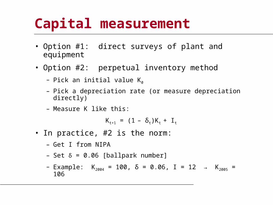
Capital measurement
• Option #1: direct surveys of plant and equipment
• Option #2: perpetual inventory method
– Pick an initial value K0
– Pick a depreciation rate (or measure depreciation directly)
– Measure K like this:
Kt+1 = (1 – δt)Kt + It
• In practice, #2 is the norm:
– Get I from NIPA
– Set δ = 0.06 [ballpark number]
– Example: K2004 = 100, δ = 0.06, I = 12 → K2005 = 106

Labor
• Meaning: units of labor used in production (labor input)
• Why does it change? – Population growth
– Fraction of population employed, hours worked, changes in skill
• Basic measure: L = number of workers (employment)
• Adjustments for quality? Quantity? – Skill: education? other? [H = “human capital”]
– Hours: often not available [h = hours]
– Leads to an “augmented production function”:
Y = A F(K,hHL) = A Kα (hHL)1-α

Age distribution
0.0
2.0
4.0
6.0
8F
ract
ion
of P
opu
latio
n
0-4 20-24 45-49 70-74 100+Age Cohort
JapanUnited StatesWestern Europe

Age distribution
0.0
5.1
.15
Fra
ctio
n of
Po
pula
tion
0-4 20-24 45-49 70-74 100+Age Cohort
AfricaAsiaEuropeNorthern America
Latin America

Productivity and “TFP”
• Standard number– Average product of labor: Y/L
• Our number: – Total Factor Productivity: Y/F(K,L) = Y/[Kα L1-α]
• How do we measure it? – Solve the production function for A:
Y = A Kα L1-α
A = Y/[Kα L1-α] = (Y/L)/(K/L)α
• Example (US): Y/L = 33, K/L = 65: A = 33/651/3 = 8.21

GDP per capita revisited
• Where does GDP per capita come from?
Y/POP = (L/POP) (Y/L)
= (L/POP) A (K/L)α
• Reasons for high GDP per capita:
– More work: L/POP
– More productivity: A
– More capital: K/L
– Not present but could be added: skill H or hours worked h

Takeaways
• The production function links output to inputs and productivity:
Y = A Kα L1-α
• The capital input (K):
– Plant and equipment, a consequence of investment (I)
• The labor input (L):
– Population growth, age distribution, participation
– Could add skill (H) or hours per person (h)
• TFP (A) can be inferred from data on output and inputs


