
ARL-TR-8348 ● APR 2018
US Army Research Laboratory
The Gibbs Variational Method in Thermodynamics of Equilibrium Plasma: 1. General Conditions of Equilibrium and Stability for One-Component Charged Gas by Michael Grinfeld and Pavel Grinfeld
Approved for public release; distribution is unlimited.

NOTICES
Disclaimers
The findings in this report are not to be construed as an official Department of the
Army position unless so designated by other authorized documents.
Citation of manufacturer’s or trade names does not constitute an official
endorsement or approval of the use thereof.
Destroy this report when it is no longer needed. Do not return it to the originator.

ARL-TR-8348 ● APR 2018
US Army Research Laboratory
The Gibbs Variational Method in Thermodynamics of Equilibrium Plasma: 1. General Conditions of Equilibrium and Stability for One-Component Charged Gas by Michael Grinfeld Weapons and Materials Research Directorate, ARL
Pavel Grinfeld Drexel University, Philadelphia, PA
Approved for public release; distribution is unlimited.

ii
REPORT DOCUMENTATION PAGE Form Approved
OMB No. 0704-0188
Public reporting burden for this collection of information is estimated to average 1 hour per response, including the time for reviewing instructions, searching existing data sources, gathering and maintaining the
data needed, and completing and reviewing the collection information. Send comments regarding this burden estimate or any other aspect of this collection of information, including suggestions for reducing the
burden, to Department of Defense, Washington Headquarters Services, Directorate for Information Operations and Reports (0704-0188), 1215 Jefferson Davis Highway, Suite 1204, Arlington, VA 22202-4302.
Respondents should be aware that notwithstanding any other provision of law, no person shall be subject to any penalty for failing to comply with a collection of information if it does not display a currently
valid OMB control number.
PLEASE DO NOT RETURN YOUR FORM TO THE ABOVE ADDRESS.
1. REPORT DATE (DD-MM-YYYY)
April 2018
2. REPORT TYPE
Technical Report
3. DATES COVERED (From - To)
1 October 2017–13 March 2018
4. TITLE AND SUBTITLE
The Gibbs Variational Method in Thermodynamics of Equilibrium Plasma:
1. General Conditions of Equilibrium and Stability for One-Component
Charged Gas
5a. CONTRACT NUMBER
5b. GRANT NUMBER
5c. PROGRAM ELEMENT NUMBER
6. AUTHOR(S)
Michael Grinfeld and Pavel Grinfeld
5d. PROJECT NUMBER
5e. TASK NUMBER
5f. WORK UNIT NUMBER
7. PERFORMING ORGANIZATION NAME(S) AND ADDRESS(ES)
US Army Research Laboratory
ATTN: RDRL-WMP-C
Aberdeen Proving Ground, MD 21005
8. PERFORMING ORGANIZATION REPORT NUMBER
ARL-TR-8348
9. SPONSORING/MONITORING AGENCY NAME(S) AND ADDRESS(ES)
10. SPONSOR/MONITOR'S ACRONYM(S)
11. SPONSOR/MONITOR'S REPORT NUMBER(S)
12. DISTRIBUTION/AVAILABILITY STATEMENT
Approved for public release; distribution is unlimited.
13. SUPPLEMENTARY NOTES
14. ABSTRACT
In this report, we study the equilibrium and stability conditions of one-component charged gas using the Gibbs variational
principles. We established the general equations allowing us to analyze the equilibrium conditions of the systems, which
contain electrically charged constituents. For the sake of simplicity, technical transparency, and brevity, we limited ourselves
to the systems containing the charges of a one sign. Our approach was based on the variational principles of Gibbs, which, in
turn, are based on the concept of heterogeneous systems. The deduction of equations of equilibrium is based on the calculation
of the first energy variation of the functionals with isoperimetric constraints. We established necessary conditions of
thermodynamic stability of the corresponding equilibrium configurations and demonstrated how the concept of stability can be
applied to the classical problem of thermodynamic inequalities. We also established the novel thermodynamic inequalities,
which generalize the classical thermodynamic inequalities of Gibbs for the charges liquids or gases.
15. SUBJECT TERMS
plasma, thermodynamics, Gibbs variational principles, plasma stability, equations of state
16. SECURITY CLASSIFICATION OF: 17. LIMITATION OF ABSTRACT
UU
18. NUMBER OF PAGES
24
19a. NAME OF RESPONSIBLE PERSON
Michael Grinfeld
a. REPORT
Unclassified
b. ABSTRACT
Unclassified
c. THIS PAGE
Unclassified
19b. TELEPHONE NUMBER (Include area code)
(410) 278-7030 Standard Form 298 (Rev. 8/98)
Prescribed by ANSI Std. Z39.18

Approved for public release; distribution is unlimited.
iii
ContentsAcknowledgment iv
1. Introduction 1
2. Gibbs Method in the Integral Form 1
2.1 The Functional for One-Component Plasma 2
2.2 Basic Gibbs Variational Principle 5
2.3 First Variation and the Equilibrium Equations 5
3. Second Variation and Stability Conditions 8
3.1 Spectral Analysis of the Second Variation 9
3.2 Thermodynamic Inequalities 11
4. Conclusion 15
5. References 16
Distribution List 17

Approved for public release; distribution is unlimited.
iv
Acknowledgment
The authors are sincerely and deeply grateful to the world-class expert in plasma
physics, Dr Sergei Putvinski of Tri Alpha Energy, Inc., for his generosity in
sharing with us his unique vision on plasma problems.

Approved for public release; distribution is unlimited.
1
1. Introduction
The systems carrying electric charges in the form of plasma are widespread in
nature. Various US Army-related applications deal with different plasmas. We do
not dwell on any particular applications since we have analyzed theoretical issues
equally relevant for any of those practical applications.
Basically, we address the general problems related to thermodynamics of plasma,
including equilibrium and stability conditions for macroscopic systems containing
components in a plasma state. Of course, these general issues have been addressed
and revised in tens of classical textbooks, and certainly they will be addressed and
revised in hundreds of textbooks to come. This keeps happening for 2 main
reasons. First, the fundamentals of any discipline are full of striking
inconsistences and contradictions. These striking contradictions will never be
fully avoided, although they stay dormant, sometimes, for decades and even
centuries. Second, the number of promising and useful applications keeps
growing and requires permanent revisions of fundamentals.
Thus, we do not address all fundamental problems and contradictions; this is
simply impossible. Instead, we discuss the bare minimum of the thermodynamical
tools—only those tools that are absolutely unavoidable when dealing with the
problems of equilibrium and stability of systems containing gaseous plasmas.
There are 2 different approaches in thermodynamics, each having its own
advantages and disadvantages. Josiah Willard Gibbs made the major contributions
to each of them in his seminal treatises.1,2 Current textbooks and monograph
presentations of the thermodynamics of plasma mostly follow the Gibbs2 basic
principles of statistical thermodynamics and their subsequent development.
Landau and Lifshitz3 summarize those developments.
The approach of Gibbs,1 based on the concept of heterogeneous systems and
usage of variational principles, did not get enough attention. Here we apply the
Gibbs variational method (as we understand it) for the analysis of the simplest
possible systems containing ionized gases.
2. Gibbs Method in the Integral Form
As per the Gibbs general methodology, based on the concept of heterogeneous
systems, we have to choose the energy and entropy functionals and specify the
macroscopic degrees of freedom for the system. Consider a closed vessel
containing a gas or liquid, the material particles of which carry charges.

Approved for public release; distribution is unlimited.
2
Typically, the net charge of the system is close to zero. However, for the sake of
brevity, we assume that all the charges are the same; for instance, electrons or
negatively charged ions.
We use the Eulerian approach to describe liquid continuum media. Fortunately,
the Eulerian description is the most convenient when dealing with both the
thermodynamics of liquids and gases and also with electromagnetism.
2.1 The Functional for One-Component Plasma
Let be the volume inside the closed vessel. Let z be the mass densities per
unit volume of the gas (liquid) under study. Let be the charge density per unit
mass. The charge density q per unit volume, then, is given by the relationship
q . (1)
Let M and Q be the total mass and charge of the liquid, respectively. They are
expressed by the following integrals over the domain occupied by the charged
gaseous substance:
,M d z Q d q z M
. (2)
Let the z be the entropy density per unit mass of the electric liquid, whereas
S is the total entropy of the system; then we get
S d z
. (3)
Let the e z be the spatial distribution of the internal energy density per unit
mass of the electric liquid, whereas U is the total internal energy of the system,
as follows:
U d e z
. (4)
Similarly, we introduce be the free energy density z per unit mass of the
electric liquid, whereas F is the total internal energy of the system and other
thermodynamic functions.
The thermodynamics of the system will be completely defined when the internal
energy density e is given as a function of the mass density and the mass
entropy density , as follows:

Approved for public release; distribution is unlimited.
3
,e e . (5)
Given the function , ,e there is no need to separately choose any additional
equations of state (EOSs); like, for instance, the pressure p or the absolute
temperature T as functions of 2 macroscopic thermodynamic parameters. This
information is already contained in the function ,e and can be extracted
from this function with the help of the formula
2
, ,, , ,
e ep T
, (6)
but not the other way around. Given the function ,p we cannot recover
from it the internal energy density function , .e That is why the function
,e can be coined a complete EoS, whereas ,p or ,T are
incomplete EoSs. So, there are several incomplete EoSs, none of which contains
as much information as , .e However, several incomplete EoSs can contain
altogether as much information as one complete EoS. The advantage of the
incomplete EoSs is implied by the fact that they can be more easily extracted from
physical experiments.
One can ask, “Is there only one complete EoS for given liquid substance?” The
answer is negative. In particular, the free-energy density function ,T
contains as much information as the complete EoS function , .e Thus,
,T is also a complete EOS on its own right.
The statistical thermodynamics provides a theoretical procedure allowing us to
extract the complete EoS ,T from data related to the spectrum of existing
energy levels of the system. Calculation of the EoS still relies on an additional
hypothesis that is not that easy to justify. Fortunately, some of the important
qualitative facts can be extracted without full knowledge of the spectra.
The macroscopic Gibbs approach, based on the concept of heterogeneous
systems, does not suggest any procedure for calculating the complete EoS from
theoretical reasoning. Basically, with this approach the EoS should be extracted
from specially designed experiments dictated by the basic thermodynamic
principles, physical intuition, or a combination.
The peculiarity of the heterogeneous systems with plasma components consists in
the necessity of taking into account the nonlocal electrostatic energy as an
essential addition to the classical internal energy.
The classical, local, and additive internal energy can be presented in the form of a
single integral over the domain , occupied by the substance under study. At the
Approved for public release; distribution is unlimited.
4
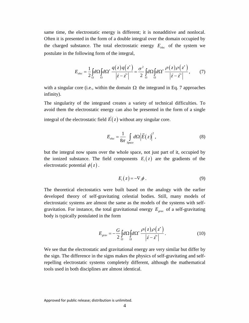
same time, the electrostatic energy is different; it is nonadditive and nonlocal.
Often it is presented in the form of a double integral over the domain occupied by
the charged substance. The total electrostatic energy elecE of the system we
postulate in the following form of the integral,
21
2 2elec
q z q z z zE d d d d
z z z z
, (7)
with a singular core (i.e., within the domain the integrand in Eq. 7 approaches
infinity).
The singularity of the integrand creates a variety of technical difficulties. To
avoid them the electrostatic energy can also be presented in the form of a single
integral of the electrostatic field 21,
8elec
Space
E d E z
without any singular core.
21,
8elec
Space
E d E z
(8)
but the integral now spans over the whole space, not just part of it, occupied by
the ionized substance. The field components iE z are the gradients of the
electrostatic potential z .
i iE z . (9)
The theoretical electostatics were built based on the analogy with the earlier
developed theory of self-gravitating celestial bodies. Still, many models of
electrostatic systems are almost the same as the models of the systems with self-
gravitation. For instance, the total gravitational energy gravE of a self-gravitating
body is typically postulated in the form
2grav
z zGE d d
z z
. (10)
We see that the electrostatic and gravitational energy are very similar but differ by
the sign. The difference in the signs makes the physics of self-gravitating and self-
repelling electrostatic systems completely different, although the mathematical
tools used in both disciplines are almost identical.

Approved for public release; distribution is unlimited.
5
In the following, we neglect the gravitational energy. We assume that the total
energy of the system totE comprises the total internal energy internal
intE and
total electrostatic energy given by the integrals
2
int ,2
tot elec
z zE E E d e d d
z z
. (11)
2.2 Basic Gibbs Variational Principle
Following Gibbs, we postulate that the thermodynamic and mechanical
parameters of the equilibrium configuration deliver the minimum (more precisely,
stationary value) to the total energy ,totE given by Eq. 11. When talking about
minimum, we must specify the mechanical and thermodynamical degrees of
freedom of the system under consideration. Quite often, it is done by specifying
allowable infinitesimal variations of certain parameters. We postulated that for
our system the virtual variation of the mass density and entropy must
keep the following integral amounts fixed:
,d z M
(12)
and
d z S
. (13)
Using the standard method of the Lagrange indefinite multipliers, we arrive at the
following unconditional variational problem for the functional :
2
,2
z zd e d d
z z
, (14)
where and are the indefinite Lagrange multipliers.
2.3 First Variation and the Equilibrium Equations
The first variation of the functional reads

Approved for public release; distribution is unlimited.
6
2 z
e z ze d
d
e
. (15)
Indeed, the functional can be presented as sum of 2 terms, as follows:
I I , (16)
where
,I d e
(17)
and
2
2
z zI d d
z z
. (18)
Varying the expressions Eqs. 17 and 18, we get, respectively,
I d e e
(19)
and
2z
I d z dz z
. (20)
The denominator 2 in the relationship Eq. 20 disappeared because in the
integrand of Eq. 18 appears twice as z and z .
Adding the relationships Eqs. 19 and 20 we arrive at the required relationship
Eq. 15 for the first variation of .
Separating the independent variations and in Eq. 15, we arrive at the
following conditions of the bulk equilibrium:
2z
e dz z
(21)
and

Approved for public release; distribution is unlimited.
7
e . (22)
Thus, we arrive at the system of 4 equations describing equilibrium
configurations: 3 integral Eqs. 12, 13, and 21, and 1 algebraic Eq. 22, with respect
to 4 unknowns: 2 spatial function ,z ,z and 2 unknown constants and
. No boundary conditions are necessary for this system.
Let us introduce an electrostatic potential ,z defined as
z
z dz z
. (23)
We then can rewrite the relationship Eq. 21 as
, ,e e . (24)
Using thermodynamic identities, Eq. 6, we can rewrite the relationship Eq. 24 as
,p
e T
. (25)
The relationship Eq. 25 can also be rewritten in terms of the free energy density
e T as
p
. (26)
The relationships Eqs. 25 and 26 are equivalent from the standpoint of
mathematics; however, depending on circumstances, one or another form appears
to be more technically convenient.
In the absence of electric field the relationship Eq. 25 implies
p
e T
. (27)
The combination on the left-hand side of Eq. 27 is the specific value (per unit
mass) of the so-called Gibbs thermodynamic potential, or the Grand
thermodynamic potential of one-component liquid substance. For heterogeneous
systems containing 2 one-component phases, this quantity also plays the role of
the chemical potential μ of the phases. In other words, the full equilibrium in the
heterogeneous system, containing 2 one-component phases—not only the
pressures and temperatures of the phases—should be equal 1 2 1 2,p p T T , but

Approved for public release; distribution is unlimited.
8
the chemical potentials of the phases 1 2 should also be equal. We do not
proceed with this discussion in this paper; it will be done later. The interested
reader should refer to the Grinfeld monograph.4
The relationship Eq. 25 shows that when dealing with electrostatic forces the
additional term , responsible for electrostatic interaction, should be included in
the equilibrium equation and in the chemical potential . This fact was known to
Gibbs,1 who established it from a different, less formal, and more intuitive
reasoning. The advantage of the reasoning, presented here, is that it allows us to
proceed with calculation of the second variation and, thus, to get the toll for
analysis of stability conditions and not just the conditions of equilibrium. This is
something that Gibbs was not able to accomplish in his time.
3. Second Variation and Stability Conditions
The main instrument in investigation of stability of heterogeneous systems is the
second energy variation. If the second variation is negative for some allowable
variations of the thermodynamics degrees of freedom, we can conclude that the
equilibrium configuration under study is unstable.
By varying the relationship Eq. 15 one more time in the vicinity of equilibrium
configuration, we arrive at the following formula of the second variation:
2 2 2
2
, 2a h d A a A ah A h
a z a zd d
z z
, (28)
where
, ,
, , ,
a z h z
A e A e A e
. (29)
For stability, the integral quadratic form 2 ,a h should be nonnegative for the
arbitrary variations satisfying the linear bulk constraints.
0, 0d a z d h z
. (30)

Approved for public release; distribution is unlimited.
9
3.1 Spectral Analysis of the Second Variation
Consider the minimum of the second variation Eq. 28 under the isoperimetric
constraints of Eq. 30 and the normalization condition
2 1.d a z
(31)
As before, we arrive at the unconditional minimization of the functional
2 2
2
2
, a z a z
z z
A a A ah A h
a h dd a h a
. (32)
In the relationship Eq. 32, , , and are the indefinite multipliers associated
with the constraints Eqs. 30 and 31.
For the first variation of this functional we get
12
12
1,
2
a z
z zA a A h d a
a h d
A a A h h
. (33)
Thus, we arrive at the nonuniform linear bulk equations
1
2
a zA a A h d
z z
(34)
and
1
2A a A h . (35)
We arrived at 5 equations, 2 Eqs. 30, plus Eqs. 31, 34, and 35, and 5 unknowns,
, , , , .a h Consider a solution of this system to be
, , , ,anda a h h , (36)
where the superscript “ ” refers to the equilibrium values of the corresponding
parameters.
So, by definition, we get the following relationships:

Approved for public release; distribution is unlimited.
10
2 1,d a z
(37)
0, 0,d h z d a z
(38)
1
2
a zA a A h d
z z
, (39)
and
1
2A a A h . (40)
Let us consider Eqs. 38, 39, and 40 as a system of 4 linear equations with 4
unknowns , , , and .a h This system is not only near but also uniform.
Therefore, it always has a trivial solution 0.a h This solution is of no
interest to us since in view of Eq. 37 we need a solution oft 0.a So, we have to
have a situation in which the system of Eqs. 17a, 18, 19 has multiple solutions.
This is possible only for some special values of γ. We call them spectral values.
In the following it is evident that the spectral values play a special role in the
analysis of stability of equilibrium
For a spectral value , let us calculate the corresponding no-vanishing values of
the unknowns , , , and .a h Let us multiply Eq. 39 by ,a Eq. 40 by h , and
integrate the resulting relationships over the volume . Then, using Eq. 17, we
get the relationships
2a z a z
d A a z d A h a z d dz z
(41)
and
2 0e ed A a h d A h
. (42)
Adding the relationships Eqs. 41 and 42, we get the relationship
2 22a z a z
d A a A h a A h d dz z
. (43)

Approved for public release; distribution is unlimited.
11
Comparing Eq. 28 with Eq. 43, we get
2 ,a h . (44)
In words, the relationship Eq. 44 says that the spectral values and the
associated nontrivial solutions of the system Eqs. 38, 39, and 40 are equal to the
extrema of the second energy variation of the system. Thus, we get the following
necessary conditions of stability. For stability all the solutions of the system
Eqs. 29, 31, 34, and 35, all the values of must be nonnegative.
We can reformulate this statement as the following:
For stability, all the spectral values of the linear uniform system
0, 0,d a z d h z
(45)
1
02
a zA a A h d
z z
, (46)
and
1
02
A a A h , (47)
with respect to the unknowns , , , anda h , must be nonnegative. In the
following we will be calling this statement the Stability Principle of Nonnegative
Spectrum.
3.2 Thermodynamic Inequalities
The problem of stability and the stability principle of nonnegative spectrum has
an immediate relation to the problem of thermodynamic inequalities. For the
analysis of thermodynamical inequalities it is convenient to rewrite Eq. 46 as the
following pair of equations:
1
02
A a A h (48)
4 0i
i a . (49)
Consider a shortwave spectrum of the system Eqs. 47–49 for which

Approved for public release; distribution is unlimited.
12
0, , ,m m m
m m mik z ik z ik za Ae h He Je . (50)
Then, Eqs. 47–49 imply the following system:
0A A A H , (51)
0A A A H J , (52)
and
2
4 0k J A . (53)
By eliminating the scalars H and J in Eqs. 51–53, we arrive at the single linear
uniform equation
22
4 0A
A k AA
(54)
with respect to the remaining constant .A
Equation 54 always has the following trivial solution:
0A . (55)
The nontrivial solutions exist only when the expression on the brackets in Eq. 54
vanishes. This obvious fact leads us to the following formula for the spectral
values :
22
4A A A
kA
. (56)
Thus, we arrive at the inequality
22
4 0
e e e
e
A A Ak
A
. (57)
If, instead of the normalization condition Eq. 31, we use
2 1,d h z
(58)
then instead of the system Eqs. 51–53, we get the system

Approved for public release; distribution is unlimited.
13
0A A A H , (59)
0A A A H J , (60)
and
2
4 0k J A . (61)
System Eqs. 59–61 leads us to somewhat different spectral values of λ.
22
2
4
4
A A A k A
A k
. (62)
Thus, we arrive at the thermodynamic inequality
22
2
40
4
A A A k A
A k
. (63)
At last, let us consider the case of the normalization condition
2 2 2 1d a h
. (64)
In this case, we arrive at the spectral system
2 0A A A H , (65)
0A A A H J , (66)
and
2
4 0k J A , (67)
which can be rewritten in the following matrix form:

Approved for public release; distribution is unlimited.
14
2
2
0 0
1 0
04 0 1
A A A
A A H
Jk
. (68)
At ,k the Eq. 68 reads
2 0 0
1 0
0 0 1 0
A A A
A A H
J
, (69)
leading to the spectrum (secular) equation
2 2
2
2 20
A A A A A
. (70)
Equation 71 has the following discriminant :
24 2 2 2
22 2 2
4
4
A A A A A
A A A
. (71)
Obviously, the discriminant is always positive, and therefore the spectrum
values are real. They will be nonnegative provided the following relationships
are satisfied:
2 0A A A (72)
and
2 0A A . (73)
Since in the inequality Eq. 73 can be an arbitrary real constant, the positiveness
of the Eigenvalues implies 2 independent inequalities:
0, 0e eA A . (74)
Thus, in the asymptotics k we arrive at the 3 classical thermodynamic
inequalities of Eqs. 72, 73, and 74.

Approved for public release; distribution is unlimited.
15
4. Conclusion
We established general equations allowing analysis of the equilibrium
configurations of the systems containing electrically charged constituents. For the
sake of simplicity, technical transparency, and brevity, we limited ourselves to the
systems containing charges of a one sign. Our approach was based on the
variational principles of Gibbs, which are, in turn, based on the concept of
heterogeneous systems. The deduction of the equation of equilibrium is based on
the calculation of the first energy variation of the functionals with isoperimetric
constraints. We arrived at the system of 4 equations describing equilibrium
configurations: 3 integral Eqs. 12, 13, and 21 and one algebraic Eq. 22 with
respect to 4 unknown: 2 spatial functions ,z ,z and 2 unknown
constants, and . No boundary conditions are necessary for this system.
We then established the necessary conditions of thermodynamic stability of the
corresponding equilibrium configuration. Our approach is based on the derivation
and analysis of the second variation, which is given by the relationship Eq. 28,
which uses the notation Eq. 29. The second variation appears in the quadratic
integral form, which should be analyzed in conjunction with 2 linear integral
constraints of the isoperimetric type in Eq. 30.
We demonstrated how the concept of stability can be applied to the classical
problem of thermodynamic inequalities. We also established the novel
thermodynamic inequalities Eqs. 57 and 63, which generalize the classical
thermodynamic inequalities of Gibbs for the charges liquids or gases.
Approved for public release; distribution is unlimited.
16
5. References
1. Gibbs JW. On the equilibrium of heterogeneous substances. Transactions of
the Connecticut Academy of Arts and Sciences. 1874–1878;3:108–248, 343–
524.
2. Gibbs JW. Elementary principles in statistical mechanics. New York (NY):
Charles Scribner and Sons; 1902.
3. Landau LD, Lifshitz EM. Statistical physics. Oxford (UK): Butterworth-
Heinemann; 1980.
4. Grinfeld MA. Thermodynamic methods in the theory of heterogeneous
systems. London (UK): Longman; 1991.

Approved for public release; distribution is unlimited.
17
1 DEFENSE TECHNICAL
(PDF) INFORMATION CTR
DTIC OCA
2 DIR ARL
(PDF) IMAL HRA
RECORDS MGMT
RDRL DCL
TECH LIB
1 GOVT PRINTG OFC
(PDF) A MALHOTRA
9 JOHNS HOPKINS UNIV
(PDF) K RAMESH
4 SANDIA NATL LAB
(PDF) J NIEDERHAUS
A ROBINSON
C SIEFERT
39 ARL
(PDF) RDRL D
M TSCHOPP
RDRL DP
T BJERKE
RDRL VTM
M HAILE
RDRL WM
B FORCH
J MCCAULEY
S SCHOENFELD
RDRL WML H
B SCHUSTER
RDRL WMM
J BEATTY
RDRL WMM B
G GAZONAS
D HOPKINS
B LOVE
B POWERS
T SANO
RDRL WMM E
J SWAB
RDRL WMM G
J ANDZELM
RDRL WMP A
S BILYK
W UHLIG
J CAZAMIAS
P BERNING
M COPPINGER
K MAHAN
C ADAMS
RDRL WMP B
C HOPPEL
T WEERASOORIYA
RDRL WMP C
R BECKER
D CASEM
J CLAYTON
M GREENFIELD
R LEAVY
J LLOYD
S SEGLETES
A TONGE
C WILLIAMS
S SATAPATHY
A SOKOLOW
RDRL WMP D
R DONEY
C RANDOW
J RUNYEON
G VUNNI

Approved for public release; distribution is unlimited.
18
INTENTIONALLY LEFT BLANK.


