
The Gender Earnings Rift Assessing Hourly Earnings
Distributions of Males and Females using Structured
Additive Distributional Regression
Alexander Sohn (University of Gottingen, Netherlands)
Paper prepared for the 34
th IARIW General Conference
Dresden, Germany, August 21-27, 2016
Session 5 (Plenary): New Approaches to Studying the Causes and Consequences of Poverty, Inequality, Polarization,
and Social Conflict
Time: Thursday, August 25, 2016 [Morning]

The Gender Earnings RiftAssessing Hourly Earnings Distributions of Males and Females
using Structured Additive Distributional Regression
Alexander Sohn∗1
1Chair of Statistics, University of Gottingen
Version 0.3Last changes: 4th July 2016
Preliminary!
Abstract
This paper reconsiders the old issue of gender related discrimination with respect to
labour earnings. Rather than employing a labour definition based on payment, we employ
an activity based definition based on Margaret Reid’s Third Party Criterion. Moreover, we
assesses discrimination on the grounds of full conditional wage distributions using Structured
Additive Distributional Regression instead of just their conditional means.
Examining earnings discrimination with respect to gender in Germany in 2013, we find
that gender wage discrimination is greatly exacerbated if considered in such a framework, as
women are faced not only with a lower expected pay, but also with a more unequal distribution
as well as a higher workload of unpaid activities. Thus we find that pecuniary discrimination
is not confined to a wage gap in the region of 21% as found using a conventional approach but
rather constitutes an earnings rift between 46% and 61% depending on the degree of aversion
of inequality considered.
JEL-Classification: C13, C21, J16, J31, J71
Keywords: Inequality; Earnings Distribution; Discrimination; Gender Pay Gap; Struc-
tured Additive Distributional Regression;
∗Corresponding author: [email protected].
1

1 Introduction
Analysing the discrepancies between the labour of men and women is arguably as old as economics
itself. Clay tablets from a Mesopotamian city state yield accounts of factor inputs and grain outputs
that consider “female labour days” hinting at an analytical discrepancy between the labour of men
and women in an economic context as early as 2,200-2,100 B.C. (Nissen et al., 1993, p.54).
Since then economics has produced a vast literature on gender related questions. One of its most
prominent branches has addressed the issue of pecuniary discrimination between the labour effort of
men and women. Most of these analyses are focussed on the contemplation of wage discrimination
caused by the “malfunctioning of the labour market” (Liu, 2015, p.2) in the sense that employers
discriminate against women leading to a lower expected wage for women compared to equally
qualified men. Therefore, most such wage gap analyses implicitly use a definition of work as those
activities which are remunerated on the labour market.
Yet, this definition is problematic as it effectively imposes a dichotomy which includes some activit-
ies while excluding other activities depending on whether money was paid and not on the grounds
of the nature of the activity. Given that many societies feature a division of labour that sees
predominantly female labour discounted as “women’s work” that doesn’t need to be paid, this
problem is particularly important for the assessment of gender discrimination. This paper thus
proposes to use a broader work definition of work that is closer to the semantics of the origins
of the word labour which implied toil and exertion.1 Specifically, we categorise activities as work
according to the Third Party Criterion proposed by the pioneering work of Margaret Reid (1934).
A second aspect which we address in this paper is that wage gap analyses are generally focussed
on the difference in the expected outcome for men and women when controlling for some explan-
atory variables in a Mincer-type wage equation. While straight forward, such an approach has the
drawback that it neglects the underlying conditional distributions. Yet as soon as the preferences
are not indifferent to aspects of these distributions any assessment of the magnitude of discrim-
ination should contemplate the distributional nature of earnings. This paper proposes structured
additive distributional regression to estimate full conditional hourly earnings distributions. Using
the conditional distributions, we are able to estimate welfare measures that account not only for
differences in expected incomes but also for the differences in the degrees of inequality associated
with the earnings distribution as in Sen (1976).
1The etymology of the word labour connects it to the Middle English labouren, the Old French laborer and theLatin laborare. The word implies an activity inducing fatigue of the body or of the mind, either in doing or suffering.This stands in contrast to the Latin word opera that can also be translated as labour but which has a connotationtowards work conceived as a creative process which we admire - and thus pay money for it to be done. It couldthus be argued that conventional labour market analysis is focussed on an operare conception of work, while webase ours on a concept more akin to laborare.
2

The term we propose for the enhanced concept of gender discrimination incorporating an activity-
based definition of work and a distribution-based earnings comparison is gender earnings rift. It
should be pointed out at the outset of this paper, that the results presented are intended as a
complement to and not a replacement for the conventional gender wage gap approach.
Thus, this paper contributes to the literature mainly in three ways: First, it introduces the measure
of the gender earnings rift and contrasts it to the conventional concept of the gender wage gap.
Following the suggestion of “broaden[ing] income measures to non-market activities” by Stiglitz
et al. (2009, p.14), it thus broadens the central gender discrimination measure to include vital
components of non-market activities considered laborious. Second, it proposes to use Structured
Additive Distributional Regression to estimate full conditional earnings rate distributions in order
to address the issue of potential differences in the earnings distribution beyond the mean. Third,
it provides empirical results on the extent of the gender earnings rift in Germany in 2013. Using
data from the German Socio-Economic Panel (SOEP), we find that pecuniary discrimination is not
confined to a wage gap in the region of 21% as found using a conventional approach but rather an
earnings rift between 46% and 61% depending on the degree of aversion of inequality considered.
Additionally, we consider different sub-populations and find that the general pattern holds that
discrimination is significantly greater for the gender earnings rift than for conventional gender
wage gap measures.
The paper is structured as follows: In the following section, we portray the existent literature
on gender discrimination and contrast the conventional concept of the gender wage gap with the
concept of the gender earnings rift. In the subsequent section, we describe the data from the
German Socio-Economic Panel that we used in this article for our analysis. In Section 4, we
introduce structured additive distributional regression for estimating hourly earnings distributions
conditioned on a set of covariates. The results are presented in Section 5. At last, Section 6
concludes.
2 The Conception of the Gender Earnings Rift
2.1 Existing literature
2.1.1 The gender wage gap concept
The conventional economic concept of wage discrimination between men and women is focussed
on the differences in the expected wages offered (and eventually paid) by employers conditional on
3

a set of covariates. In a typical set-up, one would estimate the expected (log-)wage2 given a set of
covariates both for men and women in the following linear set-up (see Jenkins, 1994):
log(Yi) = X′iβ
M + εMi ∀ i ∈M, (1)
log(Yi) = X′iβ
W + εWi ∀ i ∈ W, (2)
where M and W denote the set of individuals in the sample who are male and female respectively
and Yi denotes the wage paid to the i-th individual while Xi is the i-th row of the design matrix
portraying the characteristics, Xi. The coefficients βM and βW capture the rates of return to
the various attributes captured in Xi. Lastly, εMi and εWi denote the residual terms for men and
women respectively.
In such a framework, wage differences between women and men can be divided up. Differences
may arise from differences in the characteristics of men and women. As the considered character-
istics are often thought to represent productivity potentials these differences are called “explained”
differences in the literature (see Fortin et al., 2011). For example, we tend to include education as
individuals with higher education levels are thought to pursue different (supposedly more difficult)
tasks than less qualified individuals and are thus awarded higher wages. This kind of wage dif-
ference is consequently often considered non-discriminatory as they simply convey different levels
of productivity of individuals. While it is generally acknowledged that the endowment of such
characteristics may in itself be discriminatory (e.g. Neal and Johnson, 1996) and some approaches
towards so called detailed decomposition have been made (e.g. Oaxaca and Ransom, 1999), the
applied research on the gender wage gap has largely left aside this issue with the main thrust
directed towards the following component of discrimination.
So called wage structure discrimination exists if and only if the coefficients βM and βW differ
systematically inducing a different expected (log-)wage for a given set of covariates Xi = xi. In
lack of any observable difference between the men and women it is assumed that the difference
must be considered discriminatory. In terms of the underlying economic model the source of
such discrimination is generally associated with the demand side of the labour market, that is
discrimination in the recruitment and payment of personnel which should be equally capable.
Lastly, differences in the wage structure of men and women may arise from differences in the
residuals εMi and εWi . Some recent publications have gone beyond abstracting from the residual by
focussing on the conditional expectation, E(log(Y ) |X = x). For example, Christofides et al. (2013)
apply quantile regression to assess wage differentials at different quantiles of the conditional wage
2Although the log-link allows for a nice interpretation in terms of elasticities, it also has some problems. Forexample, the nature of the log-link inhibits the inclusion of zero-wages. In addition, as Jenkins (1994) points out,everyday discussion are on the nature of wages and not log-wages.
4

distribution to construct counterfactual aggregate distributions. By contrast, van Kerm (2013)
uses maximum likelihood to estimate conditional distributions to assess gender related conditional
wage distribution differentials in Luxembourg. However, by and large the focus of applied research
has been on the assessment of expected-outcome differences with the error term treated as residual
matter which does not need to be focussed on. To date no measure of gender discrimination exists
which explicitly contemplates distributional differences at a disaggregated level in the standard
framework allowing for a multitude of (potentially continuous) variables.
2.1.2 The gender wage gap in Germany
The literature on the gender pay discrimination for Germany alone has become so large that we
focus on a few recent selected studies. For an overview of the less recent literature see Hubler
(2003) and Maier (2007).
Official publications by the German Statistical Office see the unadjusted gender wage gap largely
unchanged from 2006 to 2013 at 22-23% with a significantly smaller gap in the East (Statistisches
Bundesamt, 2014). The adjusted wage gap is not provided at a yearly basis but the most recent
account from the year 2010 sees it at 7% (Statistisches Bundesamt, 2013).3
Arulampalam et al. (2007) inquire into the existence of sticky floors and glass ceilings in Germany
and other European countries. They find that countries with a high work-life reconciliation policy
and more family-friendly work policies generally feature lower wage gaps at the bottom of the wage
distribution and wider wage gaps at the top. They also find that countries with a compressed wage
distribution generally also feature show a greater gap at the lower wage spectrum and a smaller
gap at the upper end. Concerning the impact of union coverage on sticky floors and glass ceilings
they find a positive correlation which is insignificant though in both cases.
Hirsch et al. (2010) and Hirsch and Schnabel (2012) consider differences in the labour supply of
men and women and find a systematically lower women’s elasticity of supply for women. Due to
this lower elasticity women are more prone to monopsony power and are thus paid lower wages.
In another study that also follows a monopsonistic labour market model, Hirsch et al. (2013) find
that the gender wage gap is wider in rural areas as more densely populated regional labour markets
are more competitive and hence lower the scope for discrimination by employers.
Wolf et al. (2012) consider the gender wage gap in conjunction with nationality. They find that the
gender pay gap is on average much greater than discrimination due to nationality. Furthermore
they reflect the magnitude of both gender and nationality pay gaps and find that while the latter
3The adjusted wage gap mainly controls for differences in educational attainment, work experience, workinghours as well as the occupational position and the occupational sector of employment between women and men.For a full account of the variables included see Statistisches Bundesamt (2010).
5

is smaller in business with a higher share of non-German employees the gender pay gap is even
larger in enterprises with a higher share of female employees.
Ludsteck (2014) assesses the role of gender segregation on the gender wage gap. He finds that due
to non-random sorting into jobs, establishment and occupation levels contributes around 8.2% to
the gender wage gap.
Selezneva and van Kerm (2016) consider full gender related differences in conditional wage dis-
tributions. They find that women face wage distributions which not only have lower means but
generally also feature higher levels of inequality as assessed by the Atkinson index. Applying the
inequality-sensitive wage gap measures from van Kerm (2013), they find that the wage gap is
exacerbated once inequality at the disaggregated level is considered. This paper will follow along
the same lines of thought, proposing modifications in terms of the dependent variable of interest
and the statistical technique employed.
2.2 Discrimination and the conception of the labour earnings rate
2.2.1 The conventional wage definition
One common thread running through the literature on the gender wage gap is an implicit definition
of the labour earnings rate by the wage rate concept, i.e. the average rate of payment for time
spent in a paid occupation. The wage rate Yi paid to an individual i is normally defined as
Yi =1
|Ti |
∫t∈Ti
Yi,t dt, (3)
where Yi,t denotes the wage rate paid to the individual at time t. This wage rate is averaged over
the timespan that we conceive to be working time, denoted by Ti. The cardinality of Ti is denoted
by | Ti |. By this somewhat more complicated definition, we allow for the inclusion of various
occupations which are potentially paid with different wage rates. Using standard data sources like
the SOEP, Equation 3 simply means that we take the overall earnings for a given period’s work,
i.e. the monthly earnings, and divide this by the number of hours in that period, i.e. the monthly
working hours which can be easily computed via the (actual or contractual) weekly working time.4
The implicit reasoning behind the conventional approach is that the gender wage gap analysis
4Some other studies consider the earnings and regress those on working hours and possibly some other attributeslike employment status (e.g. Blau and Kahn, 1996) to compute a standardised monthly wage rate. Although thisprocedure produces slightly different wage rates as they cease to be proportional to working time once interceptsare non-zero, the employed implicit definition of working time also only encapsulates the time spent on labour inthe conventional sense.
6
Den
sity
0 50 100 150
0.00
0.01
0.02
0.03
0.04
0.05
femalemale
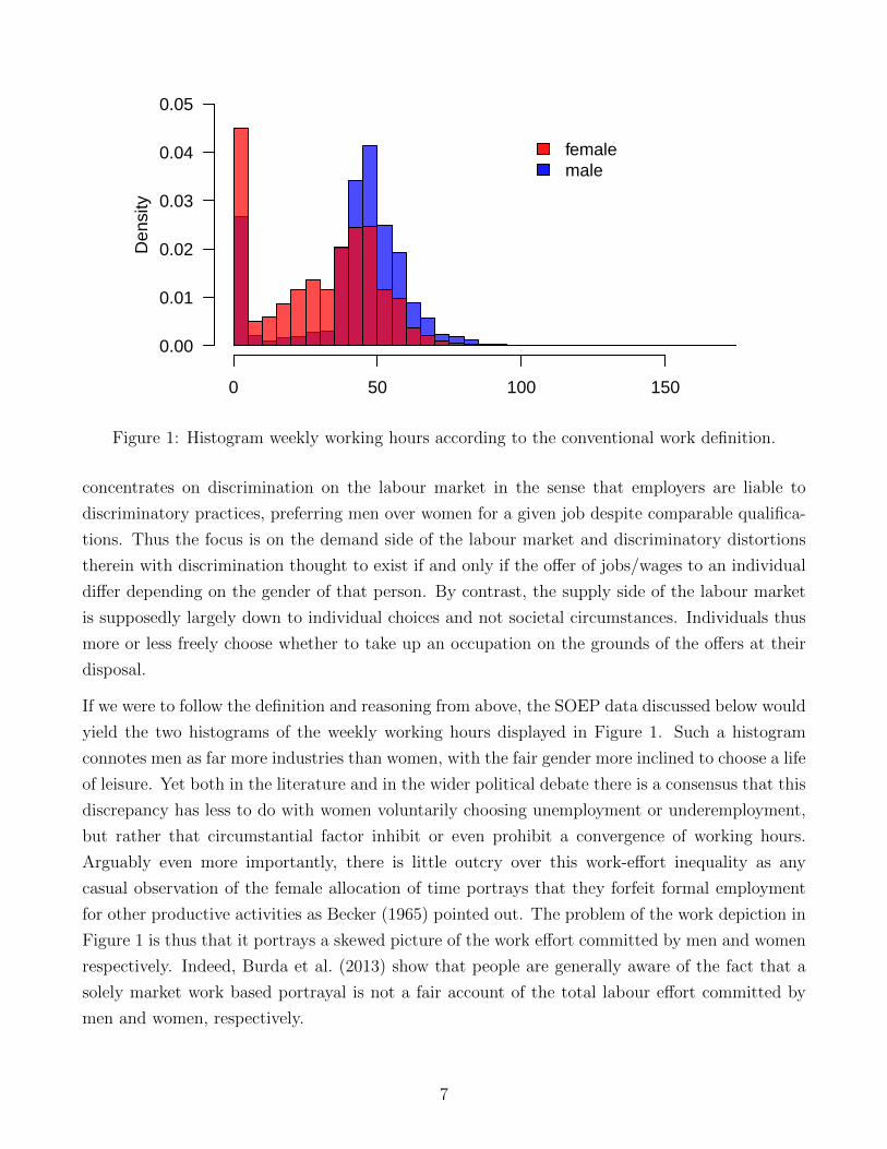
Figure 1: Histogram weekly working hours according to the conventional work definition.
concentrates on discrimination on the labour market in the sense that employers are liable to
discriminatory practices, preferring men over women for a given job despite comparable qualifica-
tions. Thus the focus is on the demand side of the labour market and discriminatory distortions
therein with discrimination thought to exist if and only if the offer of jobs/wages to an individual
differ depending on the gender of that person. By contrast, the supply side of the labour market
is supposedly largely down to individual choices and not societal circumstances. Individuals thus
more or less freely choose whether to take up an occupation on the grounds of the offers at their
disposal.
If we were to follow the definition and reasoning from above, the SOEP data discussed below would
yield the two histograms of the weekly working hours displayed in Figure 1. Such a histogram
connotes men as far more industries than women, with the fair gender more inclined to choose a life
of leisure. Yet both in the literature and in the wider political debate there is a consensus that this
discrepancy has less to do with women voluntarily choosing unemployment or underemployment,
but rather that circumstantial factor inhibit or even prohibit a convergence of working hours.
Arguably even more importantly, there is little outcry over this work-effort inequality as any
casual observation of the female allocation of time portrays that they forfeit formal employment
for other productive activities as Becker (1965) pointed out. The problem of the work depiction in
Figure 1 is thus that it portrays a skewed picture of the work effort committed by men and women
respectively. Indeed, Burda et al. (2013) show that people are generally aware of the fact that a
solely market work based portrayal is not a fair account of the total labour effort committed by
men and women, respectively.
7

One additional problem with the conventional perspective regards the treatment of those whose
wage rate is not defined as the denominator becomes zero for those completely out of paid work.
Much thought has been dedicated to the question of how to account for this problem with the
seminal paper by Heckman (1979) the most prominent example. The underlying economic ra-
tionale of the now widely applied Heckman correction is that economic agents may choose in a
non-random manner not to enter the sub-population of people with paid employment and thus
a defined wage-rate. The sample of those in employment thus potentially suffers from sample
selection biases which need to be corrected for. In case of the gender wage gap, it is assumed that
predominantly women choose not to work (full-time) preferring the alternatives on disposal as
they value the additional free time to pursue other unpaid activities more highly. By this correc-
tion, some individuals are included in the sample by means of an imputed counterfactual earnings
rate based on the earnings of individuals with equivalent observable characteristics. However, for
gender discrimination the conventional definition of work, the focus on the role of employers and
the needed correction that it ensues is problematic. Numerous publications in the economic liter-
ature point out that the selection is not first and foremost based on truly free individual choices
but that the choices themselves are circumstance-induced. As Manning (2011) points out, women
usually report that they are constrained by their domestic commitments in the jobs they can ac-
cept. The overwhelmingly disproportionate allocation of domestic commitments has in turn been
ascribed to social expectations by the economic literature (e.g. Fernandez et al., 2004; Fortin, 2005;
Allmendinger, 2010).5 Hence, the literature indicates that women are disadvantaged by cultural
institutions in their potential to receive payment for their work relative to men. Ideally, an account
of discrimination should entail this disadvantage. Yet by nature of its conception the Heckman
procedure corrects for such hypothetical differences using the counterfactual scenario of the wo-
men working at an imputed wage rather than the actual observation of the women not having
any paid work at all. If this unemployment is due to discrimination, the neglect of demand-side
discrimination thus is liable to provide biased estimates of the magnitude of discrimination on the
labour market.
2.2.2 A new labour earnings rate definition
In contrast to the conventional approach of defining labour as the time spent “on the clock” of a
paying employer, we will use an alternative definition which induces a conception of the earnings
rate which differs from the conventional wage definition used. Specifically, we follow Margaret
Reid’s Third Party Criterion, by which any activity should be considered work if the “activity is
of such character that it might be delegated to a paid worker” (Reid, 1934, p.11). Thereby the
5See also Nussbaum (1999) for a more general discussion on women’s capabilities and their connection to thesocial circumstances.
8

Den
sity
0 50 100 150
0.00
0.01
0.02
0.03
0.04
0.05
femalemale
Figure 2: Histogram weekly working hours according to the Third Party Criterion.
following activities are additionally considered work even if they are not paid: errands, house work,
child care, caring for adult persons as well as repair works - i.e. activities which could in principle
be serviced by paid work.6
If we use such an activity based definition, the two unequal distributions of the workload displayed
in Figure 1 quickly unravel. The distributions observed in Figure 2 not only display a much higher
workload by both men and women on average but also show that the distributions are much
more alike with women now actually carrying a slightly larger workload. The striking discrepancy
between the two figures shows the major importance of unpaid labour and the major discrepancy
in its distribution with women still doing the lion’s share of it. If it is true true that this division
is largely down to cultural circumstances rather than free choice, the latter distribution appears to
be a more appropriate account of the relation between men’s and women’s labour commitments.
For the analysis of the pecuniary rewards for this labour we thus propose to adapt the definition of
the earnings rate accordingly. As variable of interest we thus consider the average labour earnings
rate, i.e.
Yi =1
| Ti |
∫t∈Ti
Yi,t dt, (4)
which is equivalent to to the wage rate in Equation 3 with the exception that we now consider
not only the time spent by individual i in paid labour but in activities considered labour by the
Third Party Definition, denoted by Ti. In contrast to the conventional wage-concept we conceive
numerous activities disregarded by the former as labour activities remunerated with an earnings
6Our labour definition is thus similar to the total work concept from Burda et al. (2013).
9

rate, Yi,t. In want of a better approach, we simply use an earnings rate of zero. The effect of
this is twofold. As can be seen in Figure 2, this increases the denominator for those individuals
who spend time on unpaid laborious activities. This lowers their earnings rate both in absolute
terms and relative to those who devote less time to unpaid laborious activities, c.p. Secondly, this
means that we do not constrain our analysis to those who are in paid employment but to the whole
population who pursues any of the activities mentioned above for some time, which is practically
the whole population.
Naturally, this concept has some inherent problems as well. Just as the dichotomic conventional
definition of work for leaving out important work-like aspects can be criticised, the proposed
concept can be criticised for leaving in activities which ought to be considered leisure. Following
the definition put forward by Margaret Reid, it can be criticised that at least some of the activities
of child care can hardly be seen as work as they cannot be fully outsourced to another person.
After all, parental care is different to the care of another person. To address this problem it
is naturally feasible to only account a given percentage of such work which is partly difficult
to outsource as working time (e.g. 50%). However, such percentages are likely to be arbitrary.
Following dialectical reasoning, we will consider the extreme case of considering all child care as
work which is diametrical to the conventional reasoning of not accounting for child care at all.
Additionally, it may be argued along the lines of Becker (1965) that the unpaid activities are
productive consumption and first and foremost yield utility rather than disutility. To this, one
could respond that while this is undoubtedly true, it is also true that many paid activities are
intrinsically rewarding (see England et al., 2002) - at the very least for some individuals fortunate
enough to be able to pursue academia for a living. In addition, it has been argued that a lot of the
unpaid work goes towards things which can be considered public goods, like children or cleanliness,
thus also benefiting the man (see Ponthieux and Meurs, 2015).
One may also argue along the lines of the unitary model of household behaviour, whereby one
assumes that the unpaid work is rewarded indirectly as household members cooperate and divide
the labour on a consensual basis (see Samuelson, 1956). Thus, the income is shared altruistically
within the household, so that the potential utilities via consumptive capacity derived from the
disutilities dispensed in paid work are shared equally within the household. However, this notion
not only stands in contrast to the rationale of the principle of individualism underlying standard
economic theory. The scarce empirical literature on the matter also shows that intra-household
allocation is far from equitable but rather governed by the power structures based on the paid
work’s income (see Bourguignon et al., 1993). In any case, utility and disutility, transient and
complex as they are in their nature, can hardly be operationalised for an empirical assessment of
the gender earnings rift.
Lastly, one may criticise the valuation of unpaid work with zero earnings. In the literature two
10

other methods are dominant: The opportunity cost method would estimate what the person doing
the housework would have received if the time were devoted to remunerated labour. The second
concept of replacement cost would value the work at the estimated cost that a household would
have to pay to obtain the same service on the market. In practice, one either uses the “specialist”
concept imputing the hypothetical wage for the unpaid labour using a professional’s wage for the
task at hand. Alternatively, one may use a ”generalist” concept whereby the wage of a generalist
worker is used to impute the payment for the unpaid labour (see Eurostat, 2003). Despite the
obvious advantages over the blunt approach of simply using a zero wage, we choose to do the
latter. The reason for this is twofold.
First, as pointed out above, the opportunity cost approach may neglect the fact that circum-
stances inhibit or prohibit people in general and women in particular from realising the supposed
opportunities on offer for them. Job offers may not be available by the hour (but only from a
certain number of hours per week upwards) and thus people required to do unpaid labour cannot
exchange the former for the latter. In addition, one may criticise this approach as it values activ-
ities differently depending on who pursues them. Lastly, the estimation process is full of technical
difficulties most notably the difficulty of estimating opportunity costs for those who do not work
at all. Landefeld and McCulla (2000) point to several problems with the replacement cost method.
For example, the first approach cannot account for the fact that in the household several tasks can
and are executed simultaneously. The second approach neglects the fact that several tasks cannot
be executed by a generalist worker.
The second reason is more fundamental. All the imputation based approaches use assumably ob-
served market prices for labour and extrapolate these to supposedly comparable activities which
are not remunerated. However, as we discuss below, labour market remunerations show consider-
able variation even at the highly disaggregated level. The valuation of activities must thus be seen
as stochastic, making extrapolation problematic. This problem is even enhanced by the possibility
that valuation of unpaid activities is inherently different to that of paid activities. As the humorist
Evan Esar pointedly remarked: “Housework is what a woman does that nobody notices unless
she hasn’t done it.”(Esar, 1968, p.398). If it is true that much of the valuation of an activity is
only realised in the explicit exchange for money and is undervalued, or even not valued at all, the
extrapolations proposed above are not adequate here.
2.3 Wages and stochastics at the disaggregated level
It is evident that one does not observe one single equilibrium wage for workers with equivalent
observable characteristics but rather a labour market with major deviations from the expected
wage. This is equally true for the labour earnings rate introduced above as both monthly earnings
11

and work hours (paid and unpaid) vary substantially across people with equivalent observable
characteristics. The reason for these deviations are manifold. They may be partly ascribed to
innate abilities of the individual. They may in part be down to voluntary choices of the individual
and in part to the societal circumstances facing the individual. In addition, one would probably
need to agree with “the fact that luck played a role in the outcome” (Kahneman, 2011, pp.178-179).
In light of the convoluted and complex nature and given the bounded ability of human beings (c.f.
Selten and Gigerenzer, 2002) to disentangle and understand these deviations the knowledge of the
true mechanism must be considered unkown. Thus, we believe it adequate to perceive that the
individuals implicitly conduct an “axiomatic reduction from the notion of unknown to the notion
of random” ascribing the deviations from the expected wage as chance.
However, this does not mean that women and men are indifferent to the nature of the stochastic
variations. A broad empirical literature exists on how concerned people are with distributional
aspects beyond the mean (see among others Ferrer-i Carbonell, 2005; Carlsson et al., 2005). For the
assessment of the differences in the labour earnings rate we believe that the additional dimensions
should be incorporated. Following the literature on Social Welfare (e.g. Sen, 1976; Yaari, 1988;
Duclos et al., 2003), we use the traditional Gini social evaluation function, as well as additional
social welfare functions analogously derived from measures of the generalised Gini coefficient7
(see Yitzhaki, 1979; Donaldson and Weymark, 1980) applied to the conditional labour earnings
rate distribution. Therefore, we define an Equally Distributed Equivalent Labour Earnings Rate
(EDELER) for males and females with equivalent observable characteristics as
Wx(ρ) =
∫ ∞0
k(ρ, ρ)y dFx(y), (5)
where Wx(ρ) denotes the EDELER with k(ρ, ρ) providing an ethical weight on an individuals
earning which depends on the individual’s rank in the group and on the parameter for inequality
aversion ρ (see Yitzhaki, 1979). Using the generalised Gini coefficient this can also be expressed
in the following straight forward form:
Wx(ρ) = µx(1−Gx(ρ)), (6)
where µx denotes the expected income for the conditional earnings distribution, while Gx(ρ) de-
notes its generalised Gini coefficient with inequality aversion parameter ρ.
As is standard in the literature, we consider the ratio between the variable of interest for women
and men as a measure of the degree of discrimination. For a given level of inequality aversion
and a given subpopulation selected by covariate combination X = x, we thus consider the ratio
7In the literature this is also known as the single-parameter Gini (S-Gini) or the extended Gini (E-Gini) (seeYitzhaki and Schlechtman, 2005).
12
between the EDELER for women and men, i.e.
∆x =WWx /WM
x , (7)
where WWx is the EDELER for the women in the subpopulation while WM
x denotes that for the
men. Hence, we represent the discrimination in the well known form of cents a women earns for
every Euro that a comparable man gets but considering EDELERs instead of expected earnings.
The reasoning behind this approach is that individual’s contemplate not only the absolute value
of their earnings rate but that they assess this earnings rate against the backdrop of the observed
earnings distribution in a reference group. For sake of simplicity, we simply assume that this
reference group is all individuals of the same gender with the same covariate combination as the
individual. For each group defined by covariate combination X = x, we base our assessment on the
concept of rank order weighting proposed by Sen (1973). This concept stands in contrast to the
‘optimal distribution’ concept originally put forward by Samuelson whereby “the ethical worth of
each person’s marginal dollar” is kept equal (Samuelson, 1947, p.21) which may be used to justify
the conventional approach of considering only the expected wage rate.
To give just one motivation of why this welfare approach is useful to the assessment of gender
discrimination, let us consider the proposition put forward by Kathleen Gerson that women can
either be a career women or a housewife (see Akerlof and Kranton, 2000, p.725). While taking this
binary choice at face value is possibly somewhat exaggerated, it is nonetheless an undisputed fact
that women may not be able to find the desired middle ground. It is thus feasible that women
are likely to be in a position to feel unnerved by the discrepancy between their own occupational
opportunities and the related earnings rate and the observed expected earnings rate constructed by
averaging over both career women and housewives in their reference group. By contrast, men are
unlikely to suffer from comparable life-career-related conundrums in a similar manner and more
likely to find themselves close to the expected earnings rate. As a result male earning distributions
can be expected to center more closely around their mean, while for women we would expect
greater deviations from the mean. One effect of this distributional difference are phenomenons like
the “pauperisation of motherhood” whereby women with children are faced with extremely low
earning levels (see Folbre, 2006). To leave aside this structural difference in the level of inequality
observed in the earning distributions in an assessment of the gender wage gap means to discard
the aspect of societal discrimination described by Gerson facing many women.
13

2.4 Towards an alternative perspective on discrimination
To sum up, it must be conceded “it is painfully obvious that statistics on income [...] remain based
on the unitary version of the household” (Ponthieux and Meurs, 2015, p. 999). This is particularly
obvious in the blatant neglect of unpaid laborious activities in the assessment of pecuniary gender
discrimination. To counter this and provide at least some empirical evidence, we pursue the
following strategy. We simply assess empirically what is there to observe: the pecuniary payment
awarded in a society to an individual for the spent labour, as defined by the Third Party Criterion.
Whether this payment is justified or not, whether it is flanked by amenities (enjoyable nature of
work, company car, etc.), whether it is ensued by transfers (from the family members or someone
else) or whether it has a high esteem in society is beyond the scope of the gender earnings rift
assessment - just as it is beyond the scope of the wage gap assessment.
In addition, we follow the remark of Dolton and Makepeace (1985, p.391) that “[in] principle, the
amount of sex discrimination should be deduced from a comparison of the distribution of earnings”,
by considering full earning rate distributions. As is standard, we will condition on some variables
representing individual choices and circumstances independent of gender discrimination. With
respect to variables which we consider to be down to or influenced by discriminatory circumstances,
we will take the marginal perspective as we aim for a comprehensive measure on the extent of
discrimination. For a more elaborate discussion on the reasoning underlying this choice see Section
A.2 in the appendix. Concerning the sampling universe, we consider not only those in paid
employment but also those out of paid employment.
Before we go on to putting such analysis to practice, it should be re-emphasised that our approach
rests on some far reaching assumptions pointed out above. Yet, this is obviously also the case
for the traditional gender wage gap concept. Therefore, we conceive the ensuing analysis as the
dialectic complement to the wage gap concept - far from ideal but geared to eventually derive an
improved synthesis.
3 The Data
In order to analyse nature and magnitude of distributional differences between male and female
wages in Germany, we will use the German Socio-Economic Panel (SOEP) database (see SOEP,
2014) as our primary source of data. In addition, we use the German Mikrozensus (see Section
A.1.3 in the appendix).
From the SOEP, we include persons aged between 21 and 60 years of age. In contrast to most other
studies (e.g. Dustmann and Schonberg, 2009; van Kerm, 2013; Card et al., 2013), we explicitly
14

include both people who are not in (paid) work and those who are. For the latter, we include
civil servants and the self-employed next to employees. Thus our sampling universe is the whole
population in the 40 year age range during which the majority of the population is actively involved
on the labour market.This yields 4,198 male observations and 4,984 females observations for 2013.
As dependent variable of interest, we consider the gross hourly wage, i.e. the gross earnings
divided by the hours spent working, in the comprehensive sense discussed above. Following van
Kerm (2013), it is computed by taking the gross monthly earning in the current job (including
payments for overtime) and dividing it by the number of hours worked per week multiplied by
4.32 (for week per months). As pointed out above, we include not only actual working hours but
also hours spent on making errands, house work, child care, caring for adult persons as well as
repair works for the latter - i.e. activities which could in principle and are often, at least partially,
serviced by paid work and are thus considered work according to the Third Party Criterion. In the
appendix, we also provide gross hourly wages when only considering paid work as working time.
Concerning our explanatory variables, we consider the age and the education as is standard in a
Mincer type wage equation. As noted by Morduch and Sicular (2002) the coarse discretisation of
continuous variables such as age which is commonly applied in the literature (e.g. Dustmann and
Schonberg, 2009; Selezneva and van Kerm, 2016) can pose problems. Hence, we consider age in a
continuous manner. With respect to education, we follow van Kerm (2013) and consider 4 levels of
education which are constructed as follows: the first level entails all persons who only have general
elementary education or less (i.e. those who fall under the ISCED97 categories 0-2 according to the
SOEP). The second level incorporates the persons with completed secondary education, (ISCED
level 3). The third level incorporates those with vocational training and Abitur as well as those
with a higher vocational qualification (ISCED levels 4 and 5). The last level entails all those with
completed higher education (ISCED level 6).
In addition, we consider the nationality of the person as a binary variable differentiating only
whether the person is German or not. Concerning the household characteristics of the persons,
we consider a binary variable on whether the person has children who are not yet economically
independent in the sense that the household still receives child support8 for them. Lastly, we
consider the federal state of residence.
We do not include aspects like job characteristics or the industry of employment, as these are typ-
ically strongly related to gender (see among others Folbre and Nelson, 2000; Charles and Grusky,
2004; Lillemeier, 2014). As Richard Anker (1998, p.3) points out: “Occupational segregation by
sex is extensive and pervasive and is one of the most important and enduring aspects of labor
markets around the world.” Conditioning on industry of employment or type of occupation would
8In Germany parents got between 184e and 215e per month for each child in 2013.
15

hence capture much of the variation between males and females which we consider discriminatory,
as was already pointed out by Oaxaca (1973).9 Equally, we do not condition on actual employ-
ment experience as the standard literature generally does if the data is available. Analogue to
the argument by Neal and Johnson (1996) for racial discrimination, we argue that there is dis-
crimination inherent in women’s lower levels of employment experience. Women more frequently
interrupt their careers than men for vital societal activities like child care. These interruptions are
likely to see many women gulped by the snakes or at least unable to advance the ladders in the
game-like mechanism of the labour market put forward by Manning (2003) thus leading to earning
differentials. Therefore, we take a marginal perspective rather than a conditional perspective with
respect to these latter variables. For the same reason, we also do not include individual specific
effects.
On a more general level, it is clear that the distinction between circumstance and choice constitutes
a major obstacle for the assessment of the degree of discrimination. Given the huge complexity of
the nature of human choices and the differences in circumstances the individuals are faced with
(as well as their interdependencies), any attempt to truly disentangle and identify choice-induced
and circumstance-induced differences in earnings must be considered futile. In light of this, we
will therefore follow dialectic reasoning and take the opposite view, i.e. that most choices taken by
individuals are preconditioned on the circumstances facing an individual unless there is evidence
to suppose otherwise.
Overall, we thus consider one continuous variable, two binary variables, one categorical variables
with four levels and one with 16 levels. Even if we use a rather coarse discretisation of the
continuous variable age into four ten-year periods this would yield 2048 combinations if we would
fully interact these variables. Given the samples sizes of the SOEP, it becomes quickly apparent
that regularisation is required to provide stable estimates. This regularisation is provided by the
estimation strategy, which we turn to next.
4 Methodology
For the estimation we employ the fundamental idea underlying all regression techniques that
individuals close to one another in the covariate space should have a similar earnings distribution.
In other words, if the covariate vector x1 of one individual does not deviate much from the covariate
vector of a second individual x2, then the two individuals’ earnings distributions Dx1 and Dx2
9Naturally, a relationship of these covariates with characteristics we consider, like education, may well distortour results. Yet, as Blau and Kahn (2016) point out, at least education and experience seem to work primarilywithin the industry of employment and type of occupation so that exclusion of the latter hardly distorts the resultsof the former.
16

should adhere to a similar form. In order to make an estimation feasible, we use the well established
idea of imposing an additive structure onto the covariate effects.
In order to allow for potential differences in the wage impact of the covariates on the wage distri-
butions for males and females, we will run two separate regressions for males and females, with
each regression specified as follows.
4.1 A generic representation for the predictors
As a general framework we consider structured additive distributional regression (SADR) (Klein
et al., 2015) whereby the distribution of wages, Dx, is conditioned on a set of covariates, x. The
conditional distribution is assumed to follow a parametric form. Thus, the conditional distribution
can be written in the form D(θ1(x), . . . , θK(x)), where θk(x) is the k-th parameter in the parametric
distribution and is conditioned on the covariate combination of the specific stratum. For notational
brevity we will drop the suffix (x) in the following. Additionally, we define θ = θ1, . . . , θK .
In this paper, we use the following generic representation for every parameter of the distribution:
Each parameter θk can be linked to a structured additive predictor ηθk via a suitably specified
link function, gk, mapping the predictor into the parameter space such that θk = g−1k (ηθk). The
predictor ηθk can be specified in the following form:
ηθk = βθk0 + f θk1 (x) + . . .+ f θkJk (x), (8)
where βθk0 represents the intercept of the predictor and the functions f θkj (x), j = 1, . . . , Jk, can
capture both linear and non-linear effects of single or multiple elements of the covariate vector
x. The latter is done by means of representing the function by a suitable linear combination of
basis functions which are generally penalised such that the non-parametric estimate adheres to the
required smoothness (see Fahrmeir et al., 2013).
In our application we will use the following regression set-up for all the predictors:
ηθk = βθk0 + βθk1 kids+ βθk2 nat+ βθk3 educ2 + βθk4 educ3 + βθk5 educ4
+ f θk1 (age) + heduc · f θk2 (age) + f θkspat(region), (9)
with kids and nat binary, effect-coded variables set to unity if the person has at least one child and
has German nationality, respectively. We use education-specific intercepts by three effect-coded
variables educe, where the subscript e denotes the education level, with the first education level
taken as the base. As mentioned above age is a continuous variable expressed in years. In the
17

standard Mincer wage equation, age, as a proxy for potential experience, is incorporated by a
polynomial of degree two (see Lemieux, 2006). While this linearity in parameters has proven to
perform well for the expected (log-)income, a more flexible effect of age seemed desirable for the
possibly non-linear nature of the effect of age on the various parameters of the whole conditional
wage distribution.10 Hence, we use a flexible smooth function, based on P-splines (see Eilers and
Marx, 1996; Brezger and Lang, 2006), to model the effect of age. Thereby, f generally consists
of a number of basis functions allowing for a high degree of flexibility and a penalisation term
ensuring the desired degree of smoothness adhered to by the function. To account for different
developments over the life-span depending whether the person has enjoyed higher education and
interaction with the effect-coded variable heduc which is unity if the person has a degree in higher
education, i.e. if the ISCED level is 6 according to the SOEP.
In order to capture differences between the economic dynamism of different federal states in Ger-
many, we include a hierarchical spatial effect, such that:
f θkspat(region) = β6east+ γregion, (10)
where east is an effect-coded binary variable that is unity if the federal state is situated in the East,
thus capturing the difference between the former Federal Republic of Germany and the German
Democratic Republic. The state-specific random effect is denoted γregion and accounts for variations
across individual states. For the random effect we impose a Gaussian prior centred around zero.
By incorporating this region specific term we capture the effect of contemporary region specific
effects such that past-unemployment does not induce an effect via the contemporary economic
background facing workers.
In our application, we thus condition on a handful of aspects which we believe to be identifiable
and independent from gender-related circumstances. This entails two variables which we regard
as choices that are by and large independent of gender discrimination in contemporary Germany:
the individual’s choice of whether to have children and which federal state to live in. In addition,
we condition on two variables which we consider as circumstances that are equally independent of
gender discrimination: whether the individual has German nationality as well as the individual’s
age. Lastly, we consider a hybrid of the two - education. We conceive education free of discrimina-
tion in Germany such that dependent on his/her aptitude (which we consider a non-discriminatory
circumstance) the individual is free to choose the education irrespective of the gender.
Naturally, this leaves out many important variables which, be they based on choices or circum-
stances, will affect the individual’s wages independently of the gender. Next to the issues of data
10Using the DIC as a model selection criterion we show the non-linear approach to be superior over the linearapproach - see Section Section A.11 in the appendix.
18
availability and model stability, we do not include further variables on the grounds that the mar-
ginal perspective which we take with respect to the left-out variables emulates the individual’s
perspective, who we conceive to see the world through the eyes of a person with bounded cognitive
abilities. To such a person many influences are likely to go unnoticed and much of the variation in
wages which are explained by a score of different factors will seem as random. The distributions
we thus model are conditioned on variables such that they aim to represent the perceived wage
distributions for men and women with limited information at their disposal.
4.2 Parameter estimation
Estimation is performed in a Bayesian framework using Markov Chain Monte Carlo (MCMC)
techniques implemented in the software BayesX (Belitz et al., 2015). See Klein et al. (2014) for
details on the estimation procedure. Concerning the coefficients’ prior distributions, we employ
non-informative flat priors for the linear effects and multivariate normal distributions for the basis
function coefficients of the smooth effects which are in turn scaled by inverse gamma hyperpriors
aimed at providing a data-driven degree of smoothness. Concerning the MCMC algorithm, we
use 200,000 MCMC realisations for burn-in and thin out the following 800,000 MCMC realisations
by a factor of 800. Thus, we use 1,000 MCMC realisations for each predictor ηθk to construct
the posterior of the predictor, which is then transformed by the corresponding link function gk
into the posterior distribution of the parameter of interest. These distributions are proper under
mild conditions (see Klein et al., 2015). For our inferential purposes we use the median from the
posterior as point estimate for the parameters in order to provide estimates for the resultant full
conditional distribution for the desired covariate combination. Using the MCMC realisations, we
also provide point-wise credible intervals giving a notion of uncertainty attached to the estimators.
For the estimation of the conditional hourly earnings distribution, we will use a Type II Dagum
distribution, which entails one parameter for the point mass at zero and follows a Type I Dagum
distribution for positive values.
4.2.1 Estimating the probability of zero wages
In order to incorporate zero-wages, we follow a two-stage strategy. In the first stage, we estimate
the probability mass of zero-wage and positive wages respectively. This is done by simple logistic
regression. In a subsequent estimation step we estimate the conditional distribution of wages
greater than zero.
First, we thus estimate the probability that a person is without any remunerated employment, π0,
either because of lack of work or the unpaid nature of the work they do. In both cases the wage
19

rate is considered zero, yielding the probability of receiving a zero-wage π0 = P (y = 0 | X = x):
g1(π0) = ηπ0 , (11)
where g1 is a logit-link and ηπ0 is the predictor as specified in Equation (9) for a given covariate
combination.
4.2.2 Estimating the density of positive earnings
As pointed out above, we use the Type I Dagum distribution which has a track record of per-
forming very well for modelling positive earnings at the aggregate level (e.g. Kleiber and Kotz,
2003; Chotikapanich, 2008).11 A natural alternative which is the work-horse distribution in the
literature is the log-normal distribution (see Flabbi, 2010), yet preliminary studies have found this
distribution to have problems in modelling conditional earning distributions (Sohn et al., 2015).
Although much more research must be done on the nature of conditional wage distributions, we
consider the Dagum distribution to be a good starting point as it allows for great flexibility in the
modelling of wage distributions.
The density of the Type I Dagum distribution is given by
p+(y | a, b, c) =acyac−1
bac(1 + (y/b)a)p+1, a ∈ R>0, b ∈ R>0, c ∈ R>0. (12)
The estimation of the three parameters a, b and c is done using the following generic predictor
set-up as discussed above:
g2(a) = ηa, (13)
g3(b) = ηb, (14)
g4(c) = ηc, (15)
where all three link functions are log-link functions ensuring a positive support for the parameters
and inducing a multiplicative connection between the covariates.
11This distribution is very similar to the Singh-Maddala distribution which has been used by Biewen and Jenkins(2005) for conditional earning distributions and by van Kerm (2013) for modelling wage rates. Yet, Kleiber and Kotz(2003) remark that the Dagum distribution generally performs slightly better than the Singh-Maddala. It shouldbe noted that other more complex distributions, like the Generalised Beta of Second Kind, have been suggested inthe literature for aggregate income distributions which outperform the Dagum distribution. However, these morecomplex distributions have so far proven to be too complex for stable estimation. A comparative study on theperformance of the fit of these various parametric alternatives would be needed though to provide more profoundassessment on this issue.
20

Overall, the estimation procedure gives us four parameters to estimate over the covariates space.
Using this parametrisation, the density of the conditional wage distribution can be expressed as a
mixture of a point-mass at zero and a continuous distribution thereafter:
p(y | π0, a, b, c) = π01{y=0} + (1− π0)p+(y | a, b, c), (16)
where p denotes the probability mass or probability density for a given wage y. For the point mass
of zero wages 1{y=0} denotes an indicator function which is unity for a wage of zero and thus gives
a probability mass of π0. For earnings greater than zero, we obtain the density as specified by the
Type I Dagum distribution.
It should be noted that currently a lot of work is being done on various other statistical ap-
proaches allowing for the estimation of conditional distributions. For a discussion of other estim-
ation strategies, see the Section A.4 in the appendix.
5 Results
In this section we consider the differences between wages for males and females in a distributional
perspective as discussed in Section 2.
5.1 Interpreting the distributional effects at the disaggregated level
As is well-known from the literature on generalised linear models, the use of link functions in
Equations (11)-(15) implies that the impact of explanatory variables varies across the covariate
space (see among others Nelder and Wedderburn, 1972). Following Fox (1987) we employ effect
displays for three different covariate combinations - see Figure 3. Subsequently we analyse some
distribution measures for these distributions.
5.1.1 Visual analysis of conditional wage distributions
First, we display the estimated wage distribution for men (D1M) and women (D1W ) with 30 years
of age, no formal education beyond primary school, no children and no German citizenship who
live in Mecklenburg-Western Pomerania in Eastern Germany, i.e. persons who we would typically
expect to be economically disadvantaged. As can be seen both for men and women there is a
considerable proportion without employment (45% and 56% for men and women respectively).
Considering only those in employment, we can observe a distribution for men which interestingly
21

D1.: 30 years, low education, no children, foreign, Mecklenburg−Western Pomerania
incs
Den
sity
Pro
babi
lity
of P
oint
Mas
s
0
0.05
0.1
0.15
0.2
0
0.1
0.2
0.3
0.4
0.5
0€/h 10€/h 20€/h 30€/h 40€/h 50€/h
femalemale
D2.: 40 years, median education, children, German, North Rhine−Westphalia
incs
Den
sity
Pro
babi
lity
of P
oint
Mas
s
0
0.05
0.1
0.15
0.2
0
0.1
0.2
0.3
0.4
0.5
0€/h 10€/h 20€/h 30€/h 40€/h 50€/h
femalemale
D3.: 50 years, high education, children, German, Bavaria
Den
sity
Pro
babi
lity
of P
oint
Mas
s
0
0.05
0.1
0.15
0.2
0
0.1
0.2
0.3
0.4
0.5
0€/h 10€/h 20€/h 30€/h 40€/h 50€/h
femalemale
Figure 3: Conditional wage distribution estimates of males (blue) and females (red).
does not adhere to the standard positive skew observed in most income related distributions but is
negatively skewed. As we would expect we also see that men’s wages are higher and slightly more
dispersed than those of women.
In the centre of the figure, we display the estimated wage distribution for men (D2M) and women
(D2W ) who are forty years of age, have a completed education yielding an ISCED classification 3
or 4, have at least one child, have German citizenship and live in the populous state North Rhine-
Westphalia in the west of Germany, i.e. persons who can be considered the ”average Joe/Jane”.
As we can see the wage distributions differ substantially between men and women, not only in
their first two moments but also in the shape of the distribution. As expected, women are much
more likely to be receiving no earnings at all than men. If they are in employment their earnings
22

rate distribution is also shifted to the left of the men’s distribution, with the female distribution
also portraying a higher skewness, implying that women are much more likely to find themselves
below the expectation of their distribution.
The third set of distributions displays the wages of those who are generally associated with the
upper strata of society - 50-year-olds, with higher education, children and living in Bavaria located
in the affluent south of Germany (D3M and D3W ). It shows a much smaller probability mass for
those without employment and a much wider distribution for those in employment. Again women
generally earn a lower wage than men, with the shape differences similar to the one above, albeit
a much higher expectation and dispersion both for men and women.
One of the problems with the direct interpretation of income distributions is that they are naturally
very complex and cannot be as easily grasped as scalar distribution measures. In the following, we
will thus consider a handful of measures which may facilitate the interpretation of the distributional
differences between men and women.
5.1.2 Distributional measures of conditional wage distributions
D1M D1W D2M D2W D3M D3W
µ 3.17[2.52;3.91] 1.53[1.11;2.10] 8.45[7.55;9.41] 3.72[3.25;4.17] 20.13[17.69;22.97] 9.92[8.28;12.55]G(ρ=2) 0.22[0.16;0.30] 0.29[0.23;0.36] 0.21[0.18;0.25] 0.34[0.31;0.38] 0.27[ 0.23; 0.32] 0.45[0.39; 0.52]G(ρ=3) 0.79[0.73;0.83] 0.86[0.81;0.88] 0.42[0.37;0.46] 0.66[0.60;0.71] 0.40[ 0.34; 0.46] 0.64[0.58; 0.70]G(ρ=4) 0.84[0.82;0.86] 0.84[0.80;0.86] 0.51[0.46;0.56] 0.76[0.71;0.81] 0.47[ 0.40; 0.53] 0.72[0.66; 0.77]W(ρ=2) 2.47[1.87;3.12] 1.08[0.78;1.53] 6.68[5.93;7.49] 2.43[2.09;2.82] 14.66[12.65;16.90] 5.40[4.57; 6.45]W(ρ=3) 0.68[0.45;1.00] 0.22[0.14;0.37] 4.94[4.28;5.66] 1.27[0.97;1.64] 12.12[10.21;14.18] 3.59[2.91; 4.30]W(ρ=4) 0.51[0.38;0.70] 0.25[0.20;0.32] 4.17[3.51;4.88] 0.88[0.63;1.19] 10.71[ 8.85;12.68] 2.78[2.20; 3.43]
Table 1: Some distribution measures for 3 conditional wage distributions
In the first row of Table 1, we display the expected values (µ) for the six underlying wage distribu-
tions under consideration. This would be the measure of interest if there were no aversion against
inequality, i.e. W(ρ=0), and which is used in conventional analysis. In the squared brackets we
display the 95% credible intervals. Little surprisingly, we can observe that for all three groups
the expected wage is lower for females. The literature is full of such analyses and generally ar-
rives at the same result - that there is wage discrimination between women and men. In terms
of magnitude, the results in the literature generally find a smaller degree of discrimination, due
to the fact that they neither consider those without any employment nor the work done outside
employment on the labour market.
As we discussed in Section 2.3, it is important to go beyond the “one-dimensional straightjacket”
(Cowell, 2011) of expected wage analysis and consider wages’ stochastic nature. Here, we will
focus on one additional distributional aspect in particular - the inequality associated with the
23

distribution.12 To this end, we consider the Gini coefficient (G), which is generally the most
widely used inequality measure (see Cowell, 2000). Rather than just using the conventional Gini
coefficient, we display the Gini in its extended form of the generalised Gini coefficient, where the
parameter ρ yields the level of inequality aversion. While ρ = 2 yields the conventional Gini
coefficient, higher values of ρ reflect rising inequality aversion such that ρ → ∞ would yield the
attitude of a Max-Min decision maker. By contrast, ρ→ 1 would reflect an attitude of somebody
who is indifferent to inequality, which is equivalent to considering the expected earnings. In
addition to the conventional Gini coefficient, we also display the coefficient for two higher levels
of inequality aversion (ρ = 3 and ρ = 4) as findings from Ebert and Welsch (2009) indicate that
inequality aversion is higher than implied by the standard Gini coefficient with ρ = 2.
As expected, we observe in Table 1 that the inequality according to the Gini coefficient is greater
among wage distributions of women than among that of men. This difference is consistent across
all inequality aversion parameters and significant13 at the 5% level in most cases (with the major
exception being the first case). If we regard inequality in the conditional wage distribution as
undesirable, which despite some heterogeneity can generally be assumed according to the literature
(e.g. Bellemare et al., 2008), this further disadvantage for women should be considered in an
analysis of discrimination.
To this end, we use the standard social welfare concepts and display the Equally Distributed
Equivalent Labour Earnings Rate (W) discussed in Section 2.3, which takes into account both
the expected level and the inequality attached of the earnings distribution under consideration.
While the differences between males and females of this measure are treated in more detail below,
a quick glance at the table already shows that the ratios between the selected males and females
are generally greater than for the simple mean.
5.1.3 Assessing the magnitude of discrimination
As portrayed in Section 2.3, we use the ratio of both expected earning rates as well as the welfare
measures incorporating inequality to get an impression of the magnitude of discrimination for the
three groups under consideration. As Table 2 shows, the discrepancy is larger once we consider an
activity-based work definition, include those out of employment and use the EDELER.
Focussing on the group with the average men and women (D2.), the discrimination measure is 75
cents to the Euro if we consider a conventional work definition and exclude all zero-incomes (µconv0 ).
The discrepancy widens to around 49 cents to the Euro once considering work definition based on
12Note that it is of course also possible to consider additional aspects like polarisation - see Section A.7.13We use the term “significant” in the sense that according to the posterior belief the chance of the specified
alternative is assessed to be below a level of α.
24
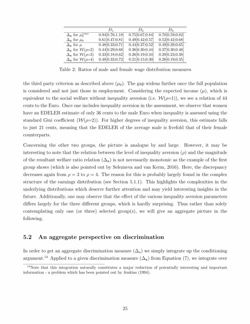
D1. D2. D3.
∆x for µconv0 0.94[0.76;1.18] 0.75[0.67;0.84] 0.70[0.59;0.82]
∆x for µ0 0.61[0.47;0.81] 0.49[0.42;0.57] 0.52[0.42;0.68]∆x for µ 0.48[0.33;0.71] 0.44[0.37;0.52] 0.49[0.39;0.65]∆x for W(ρ=2) 0.44[0.29;0.68] 0.36[0.30;0.44] 0.37[0.30;0.46]∆x for W(ρ=3) 0.33[0.18;0.62] 0.26[0.19;0.34] 0.29[0.23;0.38]∆x for W(ρ=4) 0.48[0.33;0.72] 0.21[0.15;0.30] 0.26[0.19;0.35]
Table 2: Ratios of male and female wage distribution measures
the third party criterion as described above (µ0). The gap widens further once the full population
is considered and not just those in employment. Considering the expected income (µ), which is
equivalent to the social welfare without inequality aversion (i.e. W(ρ=1)), we see a relation of 44
cents to the Euro. Once one includes inequality aversion in the assessment, we observe that women
have an EDELER estimate of only 36 cents to the male Euro when inequality is assessed using the
standard Gini coefficient (W(ρ=2)). For higher degrees of inequality aversion, this estimate falls
to just 21 cents, meaning that the EDELER of the average male is fivefold that of their female
counterparts.
Concerning the other two groups, the picture is analogue by and large. However, it may be
interesting to note that the relation between the level of inequality aversion (ρ) and the magnitude
of the resultant welfare ratio relation (∆x) is not necessarily monotonic as the example of the first
group shows (which is also pointed out by Selezneva and van Kerm, 2016). Here, the discrepancy
decreases again from ρ = 3 to ρ = 4. The reason for this is probably largely found in the complex
structure of the earnings distribution (see Section 5.1.1). This highlights the complexities in the
underlying distributions which deserve further attention and may yield interesting insights in the
future. Additionally, one may observe that the effect of the various inequality aversion parameters
differs largely for the three different groups, which is hardly surprising. Thus rather than solely
contemplating only one (or three) selected group(s), we will give an aggregate picture in the
following.
5.2 An aggregate perspective on discrimination
In order to get an aggregate discrimination measure (∆a) we simply integrate up the conditioning
argument.14 Applied to a given discrimination measure (∆x) from Equation (7), we integrate over
14Note that this integration naturally constitutes a major reduction of potentially interesting and importantinformation - a problem which has been pointed out by Jenkins (1994).
25

the covariate space (Ξ), i.e.
∆a =
∫x∈Ξ
∆xdFx(x) ≈∑x∈Ξ
∆xs(x), (17)
where Fx(x) denotes the distribution function of the covariates and s(x) denotes the share of
individuals in the population (both of men and women) who display the covariate combination x
in an adequately discretised covariate space (Ξ).
In our application, we use data from the German Mikrozensus (see Section A.1.3 in the appendix)
to obtain the shares in our discretised covariate space. We consider age as a finely discretised
variable on a yearly basis and the other variables in accordance with the categorisation discussed
in Section 3. See Section A.1.3 for further elaboration on the covariate distribution.
The discretised covariate space yields 20,480 covariate combinations for which we estimate the
conditional wage distribution for both men and women. From these we can derive discrimination
measures, such as the ratios presented in Table 2. The ratios can then be aggregated in accordance
with Equation (17) yielding an average ratio presented below:
µconv0 µ0 µ W(ρ=2) W(ρ=3) W(ρ=4)
∆a 0.79[0.75;0.82] 0.59[0.54;0.64] 0.54[0.49;0.59] 0.49[0.45;0.55] 0.42[0.37;0.48] 0.39[0.34;0.45]
Table 3: Average ratios of male and female wage distribution measures
As can be observed, estimates using the conventional approach yields an “adjusted” wage gap
between male and female earnings of around 21%.15 Yet this discrepancy is significantly enlarged
once considering a third party criterion based definition of work. Depending on the parameter
selected for inequality aversion the discrepancy between women and mean amounts to between 46%
and 61%.16 Indeed, based on the findings by Ebert and Welsch (2009) on inequality aversion levels
in Europe, it is the latter of the two figures which must be deemed the more appropriate of the two.
In other words the arguably still bridgeable wage gap of 21% pointed to by conventional analysis
quickly widens into a major rift two to three times the size when the underlying foundations of a
conventional work definition and a mean focussed analysis are not underpinning the assessment.
15This is only slightly lower than the official unadjusted pay gap of 22% (Statistisches Bundesamt, 2014) andconsiderably higher than the official adjusted pay gap of 7% (taking the latest available figure from 2010 -StatistischesBundesamt (see 2013)). The main reason for this later discrepancy is that we account for fewer aspects than thestatistical office, like occupation and industry. In addition it should be noted that for the official pay gap, geringfugigBeschaftigte are not considered, which who we do consider in the analysis. This group is predominantly female andlowly paid and thus likely to increase the pay gap. Other selection aspects, like age restrictions, are also likely tocontribute to the difference.
16Further inquiry into this much larger discrepancy found by the gender earnings rift may shed some light onthe paradox of declining female happiness found by Stevenson and Wolfers (2009) whereby female happiness hasdeclined relatively to that of men despite a narrowing gender wage gap.
26

5.3 Discrimination for sub-populations
In the following, we attempt to shed some light on the underlying mechanics of the results displayed
above, we will consider the discrimination measures for some subgroups of the population.
In Table 4 we show the distribution at the margin of four age groups. The four age groups we
consider are 21-30 years of age, 31-40 years of age, 41-50 years of age and 51-60 years of age. As
before, we still integrate over the rest of the covariate space as well as across age within the indicated
interval for each group. As one can see in the table, we generally observe the same pattern with
µconv0 µ0 µ W(ρ=2) W(ρ=3) W(ρ=4)
∆21−30 0.89[0.84;0.95] 0.72[0.64;0.80] 0.69[0.61;0.78] 0.70[0.61;0.81] 0.73[0.62;0.87] 0.69[0.59;0.84]∆31−40 0.80[0.77;0.83] 0.59[0.54;0.64] 0.51[0.46;0.56] 0.44[0.40;0.49] 0.31[0.27;0.36] 0.27[0.24;0.31]∆41−50 0.74[0.71;0.78] 0.56[0.52;0.61] 0.53[0.48;0.58] 0.47[0.43;0.51] 0.40[0.36;0.45] 0.37[0.33;0.42]∆51−60 0.75[0.72;0.79] 0.53[0.49;0.58] 0.47[0.43;0.51] 0.41[0.37;0.45] 0.31[0.28;0.36] 0.29[0.26;0.33]
Table 4: Average ratios of male and female wage distribution measures
the magnitude of discrimination increasing from left (conventional wage gap) to right (EDELER
with high inequality aversion). Concerning the differences between the age groups, it can generally
be observed that discrimination measured by conventional measures generally increase as the age
group increases. This is to be expected, supposing that men are in a better position to advance
their career and thus extend the wage gap. One notable and interesting variation is that the
EDELER wage difference show higher differences for the age range between 31-40 than for 41-50.
Indeed for the highest degree of inequality aversion, i.e. ρ=4), the discrepancy is even largest for
the former age range. The most probable reason for this is that during the former age span the
time required for nurturing both children and career is at its height. This aspect is discussed in
more detail below. Moreover, while between 41-50 and 51-60 there is no significant difference in
the conventional measure indicating stagnation, considering the EDELER, we observe significant
differences for ρ= 4. This indicates that while differences in average wages are stagnating in the
later stages of professional life, discrepancies in terms of inequality are still widening. One possibly
explanation for this finding is that many of those who have been out of paid work for long tracts
of time, mostly women, fail to revitalise their careers while others succeed. As a result inequalities
between those who go through long-term unemployment and/or very lowly-paid jobs and those
who do manage to obtain decent wages are generally more pronounced among women than among
men.
Secondly, we differentiate with respect to whether the person has a child currently eligible to child-
benefits, again integrating over the remaining covariate space. The corresponding discrimination
measures are displayed in Table 5. Little surprisingly, the gender discrepancy widens with children,
as one would expect given the evidence from the literature on the wage gap resulting out of
motherhood (see Ponthieux and Meurs, 2015). However, as above it may be noted that the gap
27

µconv0 µ0 µ W(ρ=2) W(ρ=3) W(ρ=4)
∆no kids 0.81[0.78;0.85] 0.65[0.59;0.71] 0.61[0.55;0.67] 0.57[0.51;0.63] 0.51[0.45;0.58] 0.47[0.42;0.54]∆kids 0.72[0.69;0.75] 0.42[0.40;0.46] 0.35[0.31;0.38] 0.28[0.25;0.31] 0.17[0.14;0.20] 0.15[0.13;0.18]
Table 5: Average ratios of male and female wage distribution measures
is even more pronounced for the EDELER, especially when considering inequality. While for the
expectation, µ, we see a shift from 61 cents to the Euro down to 35 cents to the Euro, i.e. roughly
halving the ratio, the EDELER with the highest inequality aversion, W(ρ= 4), yields a change
from 47 cents to the Euro down to only 15 cents to the Euro, such that the measure is even slashed
by two thirds. The reason for this heightened level of inequality among women can be mostly
ascribed to a large faction of women completely out of employment or in very lowly-paid part-time
occupations due to the time requirements of child care. In conjunction with those women who are
able to earn a relatively high income despite having children, a higher inequality, as measured by
the Gini coefficient, is generated.
In addition, we also consider differentiations with respect to education (higher education vs. no
higher education) and region (former West vs. East Germany). The results are displayed in Section
A.9 in the appendix. As for above, these measures abide with the observation that the gender
wage rift generally points to a larger magnitude of discrimination than the conventional gender
wage gap concept.
5.4 Testing for parametric misspecification
Lastly, we consider a standard Kolomogorov-Smirnov type test for the parametric specification
used for our modelling approach. Using an adaptation of the test proposed by Rothe and Wied
(2013), we obtain a p-value of 0.18 for men and a p-value of 0.62 for women using 1,000 bootstrap
repetition. These high p-values imply that the hypothesis that our parametric fit is adequate to
describing the nature of the conditional distributions is not rejected at any of the usual levels.
Hence, we consider our specification of the conditional earning distributions to be adequate. For
further details see Section A.10 in the appendix.
6 Conclusion
This article argued for the use of a more comprehensive conception of earnings discrimination
between males and females to complement the traditional concept of the gender wage gap. Look-
ing at gender related earnings discrimination in Germany, we show possible inroads to such a
28

comprehensive earnings discrimination analysis by considering an activity-based definition of work
(rather than a pay-based definition) as well as basing the analysis on full conditional earnings dis-
tributions (rather than just their expectation) using structured additive distributional regression.
We find that this change of view fundamentally alters the magnitude of pecuniary discrimination
of labour with respect to gender. Rather than an arguably still bridgeable wage gap of around
21%, we find a considerably wider earnings rift of between 46% and 61%, i.e. a discrepancy two to
three times the size. This analysis thus shows that much more work is left to do than is indicated
by common labour market analysis until women’s labour receives the same pecuniary valuation
as that of their male compatriots and ascriptions like the one from ancient Mesopotamia truly
become obsolete.
References
G. A. Akerlof and R. E. Kranton (2000): Economics and Identity, in: Quarterly Journal of Eco-
nomics, 115(3), pp. 715–753.
J. Allmendinger (2010): Verschenkte Potenziale? Lebensverlaufe nichterwerbstatiger Frauen,
Campus-Verl, Frankfurt.
D. W. K. Andrews (1997): A Conditional Kolmogorov Test, in: Econometrica, 65(5), pp. 1097–
1128.
R. Anker (1998): Gender and Jobs: Sex Segregation of Occupations in the World, International
Labour Organisation, Geneva.
W. Arulampalam, A. L. Booth and M. L. Bryan (2007): Is There a Glass Ceiling over Europe?
Exploring the Gender Pay Gap across the Wage Distribution, in: Industrial and Labor Relations
Review, 60(2), pp. 163–186.
A. B. Atkinson (1970): On the Measurement of Economic Inequality, in: Journal of Economic
Theory, 2(3), pp. 244–263.
G. S. Becker (1965): A Theory of the Allocation of Time, in: Economic Journal, 75, pp. 493–517.
C. Belitz, A. Brezger, N. Klein, T. Kneib, S. Lang and N. Umlauf (2015): BayesX - Soft-
ware for Bayesian Inference in Structured Additive Regression Models: Version 3.0, URL
http://www.bayesx.org.
C. Bellemare, S. Kroger and A. van Soest (2008): Measuring Inequity Aversion in a Heterogeneous
Population Using Experimental Decisions and Subjective Probabilities, in: Econometrica, 76(4),
pp. 815–839.
29

M. Biewen and S. P. Jenkins (2005): A Framework for the Decomposition of Poverty Differences
with an Application to Poverty Differences Between Countries, in: Empirical Economics, 30(2),
pp. 331–358.
F. D. Blau and L. M. Kahn (1996): International Differences in Male Wage Inequality: Institutions
versus Market Forces, in: Journal of Political Economy, 104(4), pp. 791–836.
— (2016): The Gender Wage Gap: Extent, Trends, and Explanations, in: IZA Discussion paper
series, No. 9656.
F. Bourguignon, M. Browning and Chiappori, P.A., Lechene, V. (1993): Intra Housheold Allocation
of Consumption: a A Model and Some Evidence from French Data, in: Annals of Economics
and Statistics, 29, pp. 137–156.
A. Brezger and S. Lang (2006): Generalized Structured Additive Regression Based on Bayesian
P-splines, in: Computational Statistics & Data Analysis, 50(4), pp. 967–991.
M. Burda, D. S. Hamermesh and P. Weil (2013): Total Work and Gender: Facts and Possible
Explanations, in: Journal of Population Economics, 26(1), pp. 239–261.
D. E. Card, J. Heining and P. Kline (2013): Workplace Heterogeneity and the Rise of German
Wage Inequality, in: Quarterly Journal of Economics, 128(3), pp. 967–1015.
F. Carlsson, D. Daruvala and O. Johansson-Stenman (2005): Are People Inequality-Averse, or
Just Risk-Averse?, in: Economica, 72, pp. 375–396.
M. Charles and D. B. Grusky (2004): Occupational Ghettos: The Worldwide Segregation of
Women and Men, Stanford University Press, Stanford.
V. Chernozhukov, I. Fernandez-Val and B. Melly (2013): Inference on Counterfactual Distribu-
tions, in: Econometrica, 81(6), pp. 2205–2268.
D. Chotikapanich (2008): Introduction, in: D. Chotikapanich (ed.), Modeling Income Distributions
and Lorenz Curves, pp. ix–xii, Springer, New York.
L. N. Christofides, A. Polycarpou and K. Vrachimis (2013): Gender Wage Gaps, ‘Sticky Floors’
and ‘Glass Ceilings’ in Europe, in: Labour Economics, 21, pp. 86–102.
F. A. Cowell (2000): Measurement of Inequality, in: A. B. Atkinson and F. Bourguignon (eds.),
Handbook of Income Distribution, pp. 87–166, Elsevier, Amsterdam.
— (2011): Measuring Inequality, Oxford University Press, Oxford, 3rd ed.
DIW Berlin (2014a): SOEP 2013 - Erhebungsinstrumente 2013 (Welle 30) des Sozio-oekonomischen
Panels: Haushaltsfragebogen, in: SOEP Survey Papers, No. 181.
30

— (2014b): SOEP 2013 - Erhebungsinstrumente 2013 (Welle 30) des Sozio-oekonomischen Panels:
Personenfragebogen, in: SOEP Survey Papers, No. 180.
P. J. Dolton and G. Makepeace (1985): The Statistical Measurement of Discrimination, in: Eco-
nomic Letters, 18, pp. 391–395.
D. Donaldson and J. A. Weymark (1980): A Single-Parameter Generalization of the Gini Indices
of Inequality, in: Journal of Economic Theory, 22(1), pp. 67–86.
J.-Y. Duclos, V. Jalbert and A. Araar (2003): Classical Horizontal Inequity and Reranking: an
Integrating Approach, in: Research on Economic Inequality, 10, pp. 65–100.
C. Dustmann and U. Schonberg (2009): Training and Union Wages, in: Review of Economics and
Statistics, 91(2), pp. 363–376.
U. Ebert and H. Welsch (2009): How Do Europeans Evaluate Income Distributions? An Assess-
ment Based On Happiness Surveys, in: Review of Income and Wealth, 55(3), pp. 803–819.
P. H. C. Eilers and B. D. Marx (1996): Flexible Smoothing with B-splines and Penalties, in:
Statistical Science, 11(2), pp. 89–102.
P. England, M. Budig and N. Folbre (2002): Wages of Virtue: The Relative Pay of Care Work, in:
Social Problems, 49(4), pp. 455–473.
E. Esar (1968): 20,000 Quips & Quotes: A Treasury of Witty Remarks, Comic Proverbs, Wise-
cracks, and Epigrams, Barnes & Noble, New York.
J. Esteban, C. Gradın and D. Ray (2007): Extensions of a Measure of Polarization, with an Applic-
ation to the Income Distribution of five OECD Countries, in: Journal of Economic Inequality,
5(1), pp. 1–19.
J. Esteban and D. Ray (1994): On the Measurement of Polarization, in: Econometrica, 62(4), pp.
819–851.
Eurostat (2003): Household Production and Consumption, Office for Official Publications of the
European Communities, Luxembourg.
L. Fahrmeir, T. Kneib, S. Lang and B. D. Marx (2013): Regression: Models, Methods and Ap-
plications, Springer, Berlin.
R. Fernandez, A. Fogli and C. Olivetti (2004): Mothers and Sons: Preference Formation and Female
Labor Force Dynamics, in: Quarterly Journal of Economics, 119, pp. 1249–1299.
A. Ferrer-i Carbonell (2005): Income and Well-Being: An Empirical Analysis of the Comparison
Income Effect, in: Journal of Public Economics, 89, pp. 997–1019.
31

L. Flabbi (2010): Gender Discrimination Estimation in a Search Model with Matching and Bar-
gaining, in: International Economic Review, 51(3), pp. 745–783.
N. Folbre (2006): Measuring Care: Gender, Empowerment, and the Care Economy, in: Journal of
Human Development, 7(2), pp. 183–199.
N. Folbre and J. A. Nelson (2000): For Love or Money - Or Both?, in: Journal of Economic
Perspecitves, 14(4), pp. 123–140.
N. M. Fortin (2005): Gender Role Attitudes and the Labour-Market Outcomes for Women across
OECD Countries, in: Oxford Review of Economic Policy, 21(3), pp. 416–438.
N. M. Fortin, T. Lemieux and S. Firpo (2011): Decomposition Methods in Economics, in:
O. Ashenfelter and D. E. Card (eds.), Handbook of Labor Economics, Vol. 4A, pp. 1–102,
North-Holland, Amsterdam.
J. Fox (1987): Effect Displays for Generalized Linear Models, in: C. C. Clogg (ed.), Sociological
Methodology, vol. 17, pp. 347–361, American Sociological Association, Washington D.C.
C. Gradın (2000): Polarization by Sub-populations in Spain, 1973-91, in: Review of Income and
Wealth, 46(4), pp. 457–474.
J. J. Heckman (1979): Sample Selection Bias as a Specification Error, in: Econometrica, 47(1), p.
153.
B. Hirsch, M. Konig and J. Moller (2013): Is There a Gap in the Gap? Regional Differences in
the Gender Pay Gap, in: Scottish Journal of Political Economy, 60(4), pp. 412–439.
B. Hirsch, T. Schank and C. Schnabel (2010): Differences in Labor Supply to Monopsonistic Firms
and the Gender Pay Gap: An Empirical Analysis Using Linked Employer-Employee Data from
Germany, in: Journal of Labor Economics, 28(2), pp. 291–330.
B. Hirsch and C. Schnabel (2012): Women Move Differently: Job Separations and Gender, in:
Journal of Labor Research, 33(4), pp. 417–442.
T. Hothorn, T. Kneib and P. Buhlmann (2014): Conditional Transformation Models, in: Journal
of the Royal Statistical Society: Series B (Statistical Methodology), 76(1), pp. 3–27.
O. Hubler (2003): Geschlechtsspezifische Lohnunterschiede, in: Mitteilungen aus der
Arbeitsmarkt- und Berufsforschung, 36(4), pp. 539–559.
S. P. Jenkins (1994): Earnings Discrimination Measurement: A Distributional Approach, in:
Journal of Econometrics, 61(1), pp. 81–102.
D. Kahneman (2011): Thinking, Fast and Slow, Farrar, Straus and Giroux, New York.
32

C. Kleiber and S. Kotz (2003): Statistical Size Distributions in Economics and Actuarial Sciences,
Wiley, Hoboken.
N. Klein, M. Denuit, S. Lang and T. Kneib (2014): Nonlife Ratemaking and Risk Management
with Bayesian Generalized Additive Models for Location, Scale, and Shape, in: Insurance: Math-
ematics and Economics, 55, pp. 225–249.
N. Klein, T. Kneib and S. Lang (2015): Bayesian Generalized Additive Models for Location,
Scale and Shape for Zero-Inflated and Over-Dispersed Count Data, in: Journal of the American
Statistical Association, 110(509), pp. 405–419.
J. S. Landefeld and S. H. McCulla (2000): Accounting for Nonarket Household Production within
a National Accounts Framework, in: Review of Income and Wealth, 46(3), pp. 289–307.
T. Lemieux (2006): The “Mincer Equation”. Thirty years after Schooling, Experience, and Earn-
ings, in: S. Grossbard (ed.), Jacob Mincer. A Pioneer of Modern Labor Economics, pp. 127–145,
Kluwer Academic, Boston.
S. Lillemeier (2014): Der Entgeltgleichheit einen Schritt naher, Bundesministerium fur Familie,
Senioren, Frauen und Jugend, Berlin.
K. Liu (2015): Explaining the Gender Wage Gap: Estimates from a Dynamic Model of Job Changes
and Hours Changes, in: IZA Discussion paper series, No. 9255.
J. Ludsteck (2014): The Impact of Segregation and Sorting on the Gender Wage Gap: Evidence
from German Linked Longitudinal Employer-Employee Data, in: ILR Review, 67(2), pp. 362–
394.
J. Machado and J. Mata (2005): Counterfactual Decompostion of Changes in Wage Distributions
Using Quantile Regression, in: Journal in Applied Econometrics, 20(4), pp. 445–465.
F. Maier (2007): The Persistence of the Gender Wage Gap in Germany, in: Harriet Taylor Mill-
Institut fur Okonomie und Geschlechterforschung, Discussion Paper 01.
A. Manning (2003): Monopsony in Motion: Imperfect Competition in Labor Markets, Princeton
University Press, Princeton.
— (2011): Imperfect Competition in the Labor Market, in: O. Ashenfelter and D. E. Card (eds.),
Handbook of Labor Economics, Vol. 4B, North-Holland, Amsterdam.
J. Morduch and T. Sicular (2002): Rethinking Inequality Decomposition, with Evidence from
Rural China, in: The Economic Journal, 112(476), pp. 93–106.
D. A. Neal and W. R. Johnson (1996): The Role of Premarket Factors in Black-White Wage
Differentials, in: Journal of Political Economy, Vol. 104(5), pp. 869–895.
33

J. A. Nelder and R. W. M. Wedderburn (1972): Generalized Linear Models, in: Journal of the
Royal Statistical Society: Series A (General), 135(3), pp. 370–384.
H. J. Nissen, P. Damerow and R. K. Englund (1993): Ancient Bookkeeping: Early Writing and
Techniques of Economic Admistration in the Ancient Near East, The University of Chicago
Press, Chicago.
M. C. Nussbaum (1999): Sex & Social Justice, Oxford University Press, Oxford.
R. L. Oaxaca (1973): Male-Female Wage Differentials in Urban Labor Markets, in: International
Economic Review, 14(3), pp. 693–709.
R. L. Oaxaca and M. R. Ransom (1999): Identification in Detailed Wage Decompositions, in:
Review of Economics and Statistics, 81(1), pp. 154–157.
S. Ponthieux and D. Meurs (2015): Gender Inequality, in: A. B. Atkinson and F. Bourguignon
(eds.), Handbook of Income Distribution, pp. 981–1146, Elsevier, Amsterdam.
M. G. Reid (1934): Economics of Household Production, John Wiley, New York.
C. Rothe and D. Wied (2013): Misspecification Testing in a Class of Conditional Distributional
Models, in: Journal of the American Statistical Association, 108(501), pp. 314–324.
P. A. Samuelson (1947): Foundations of economic analysis, Harvard University Press, Cambridge.
— (1956): Social Indifference Curves, in: Quarterly Journal of Economics, 70(1), pp. 1–22.
E. Selezneva and P. van Kerm (2016): A Distribution-Sensitive Examition of the Gender Wage
Gap in Germany, in: Internal Working Paper, 14(1), pp. 21–40.
R. Selten and G. Gigerenzer (2002): Bounded Rationality: The Adaptive Toolbook, MIT Press,
Cambridge (Mass.) and London.
A. K. Sen (1973): On Economic Inequality, Oxford University Press, Oxford.
— (1976): Real National Income, in: Review of Economic Studies, 43(1), pp. 19–39.
SOEP (2014): Socio-oeconomic Panel Study (SOEP), data of the years 1984-2013, version 30, doi:
10.5684/soep.v30.
A. Sohn, N. Klein and T. Kneib (2015): A Semiparametric Analysis of Conditional Income Dis-
tributions, in: Schmollers Jahrbuch, 135(1), pp. 13–22.
D. M. Stasinopoulos and R. A. Rigby (2007): Generalized Additive Models for Location, Scale
and Shape (GAMLSS) in R, in: Journal of Statistical Software, 23(7), pp. 1–46.
34

Statistisches Bundesamt (2010): Verdienstunterschiede zwischen Mannern und Frauen, Stat-
istisches Bundesamt, Wiesbaden.
— (2013): Frauenverdienste – Mannerverdienste: Wie groß ist der Abstand
wirklich?, URL https://www.destatis.de/DE/Publikationen/STATmagazin
/VerdiensteArbeitskosten/2013 03/Verdienste2013 03.html.
— (2014): Finanzen und Steuern: Lohn- und Einkommenssteuer 2010, Statistisches Bundesamt,
Wiesbaden.
B. Stevenson and J. Wolfers (2009): The Paradox of Declining Female Happiness, in: American
Economic Journal: Economic Policy, 1(2), pp. 190–225.
J. E. Stiglitz, A. K. Sen and J.-P. Fitoussi (2009): Rapport de la Commission sur la mesure des
performances economiques et du progres social, URL www.stiglitz-sen-fitoussi.fr.
P. van Kerm (2013): Generalized Measures of Wage Differentials, in: Empirical Economics, 45(1),
pp. 465–482.
E. Wolf, M. Beblo and C. Ohlert (2012): Gender and Nationality Pay Gaps in Light of Organisa-
tional Theories, in: Zeitschrift fur Betriebswirtschaft, 82(S2), pp. 69–94.
M. C. Wolfson (1994): When Inequalities Diverge, in: American Economic Review, 84(2), pp.
353–358.
M. E. Yaari (1988): A Controversial Proposal Concerning Inequality Measurement, in: Journal of
Economic Theory, 44(2), pp. 381–397.
S. Yitzhaki (1979): Relative Deprivation and the Gini Coefficient, in: The Quarterly Journal of
Economics, 93(2), p. 321.
S. Yitzhaki and E. Schlechtman (2005): The Properties of the Extended Gini Measures of Variab-
ility and Inequality, in: International Journal of Statistics, 63(3), pp. 401–433.
35

A Appendix
A.1 Data
As primary source for our data we use the SOEP database (SOEP, 2014). We use all available
waves in 2013, which provides us with 10 waves (A to J). Only taking those values for which we
have the full set-of variables, as described below, we obtain 9,182 observations.
A.1.1 Variables used
In order to obtain our dependent variable of the gross hourly wage we use the variable BDP7701
from the individual questionnaire (DIW Berlin, 2014a) to obtain the monthly earnings of the
individual.17 This is divided by 4.32 times the number of hours worked per week. As discussed
in Section 2.2, we do not only consider the hours of paid work but the hours spent on activities
which we consider work. For the former we use the the variable BDP66 , which is the actual number
of hours worked last week. The hours spent on housework, errands, care work and repair works
are taken from the answers from BDP10$$. These variables give the number of hours spent on
each type of activity for a regular weekday, a Saturday and a Sunday, which we simply sum up to
get the number of hours per week. It must be noted that these variables are likely to be rather
imprecise such that our data is affected by some considerable data related uncertainty.
For the explanatory variable age we simply use the birthyear (GEBJAHR) from the individual ques-
tionnaire and subtract it from 2013, while the sex is determined by the variable BDSEX. The binary
variable of whether a person has children that is still dependent on the household is based on
the variable BDH503 from the household questionnaire (DIW Berlin, 2014b). The variable nat is
constructed on grounds of variable BDP143 in the individual questionnaire (DIW Berlin, 2014a).
The education level is taken on grounds of the variable ISCED1318 from the PGEN variables. All
observations equal or lower than 2 (general elemantary and below) are put in the first education
category, with all observations in category 3 (middle vocational) put in the second category. All
observations with ISCED13 values 4 and 5 (vocational with Abitur and higher vocational) are in the
third group, while the highest group consists only of individuals with a value 6 (higher education).
For the spatial effect we use the variable BDBULA with the variable east set to unity for all federal
17We thus neglect aspects any transfer payments, like the Elterngeld. While this is obviously problematic in somecases it seems much more appropriate than the consideration of net-incomes, i.e. including all transfer payments(like Elterngeld), as we want to consider the remuneration of activities by a society prior to welfare considerationsas is standard in the discrimination literature.
18It should be noted that the SOEP ISCED levels are not a 100% equivalent to the ISCED levels elsewhere.
36

states formerly belonging to the German Democratic Republic, including the whole of Berlin,
which in the SOEP is equivalent to states 1-11. West Berlin is not accounted for separately.
All observations are weighted using the variable BDPHRF.
A.1.2 Observations dropped
Concerning the wage rate, we only consider those persons who for who we have a value greater
or equal to zero, i.e. all observations that are not missing, not applicable or highly improbable
according to the SOEP.
Concerning the age, we only consider person who are between 21 and 60 years of age and for whom
we have age observations.19
Concerning education, we all observations who have a value greater or equal to zero, i.e. all
observations that are not missing, not applicable or highly improbable according to the SOEP.
Concerning time spent, we drop observations who state more than 168 hours for activities per
week.
Concerning the federal state of residence, we use all observations.
Concerning the nationality, we use all observations.
Concerning the children, we use all observations.
Concerning the weight, we use all observations with a positive weight.
A.1.3 Construction of covariate distribution
For the construction of the covariate distribution in the discretised covariate space, we use data
from the German Mikrozensus provided upon request from the German Statistical Office. The
Mikrozensus entails information from around 370,000 household with 830,000 persons equivalent
to roughly 1% of the population. It thus allows for a relatively accurate account of the number of
persons in each strata as defined by our covariates.
We use the variables in the Mikrozensus to categorise our population strata emulating the cat-
egorisation based on the information (and variables) from the SOEP as closely as possible. To this
end, we proceed as follows:
19We explicitly do not exclude students or other persons currently in the process of enhancing their capital stockto further incomes later on. As long as such education breaks from employment are roughly equivalently distributedbetween males and females, which they are in the case of tertiary education (Statistisches Bundesamt, 2013), thisshould not distort the discrimination estimates as we define it.
37

For age we have yearly age brackets at our disposal allowing us a one-to-one comparison with the
variables from the SOEP. The same is possible for the categorisation into Germans and persons
of foreign nationality which is also recorded in the Mikrozensus equivalently to the SOEP. Con-
cerning the question of whether the individual has dependent children, we use information from
the Mikrozensus on whether the individual has under age children. This is not 100% equivalent to
the definition we use based on the SOEP, but should by and large give us similar results. Lastly
for education we use information on the education level with regard to job qualification (hochster
beruflicher Ausbildungsabschluss) available. The four education levels we use are constructed as
follows:
educ1 The first education level comprises all individuals who have no formal job-qualification
(ohne berufsqualifizierenden Ausbildungsabschluss) and those on whom we have no in-
formation (ohne Angabe zur Art des Abschlusses).
educ2 The second education level comprises all individuals who have the standard job qual-
ification, which in Germany is generally a completed apprenticeship (Abschluss einer
Lehre oder gleichwertiger Berufsfachabschluss).
educ3 The third education level comprises all individuals who have a higher technical technical
qualification (Meister-/Techniker oder geichwertiger Fachschul-abschluss and Fachschul-
abschluss der DDR)
educ4 The fourth education level comprises all individuals with higher education (Fachhoch-
schulabschluss and Hochschulabschluss).
Using this categorisation, we construct the covariate distribution yielding population shares for all
covariate combinations in Ξ as used in Equation 17.
A.2 Wages, Choices and Circumstances
Let Yi,t be a random variable of the earnings-rate offered and/or paid to individual i at time t. This
earnings-rate is thought to be derived from the individual’s capability to pursue a set of activities
required for some specific work at a given time and the surrounding circumstances of society via
some function w, i.e.
Yi,t = w(Ai,t,Si,t), (18)
where Ai,t is a vector denoting the set of activities which is selected from a space of possible human
activities A, while vector Si,t denotes the circumstances in a society currently facing the individual
stemming from the space of conceivable circumstance-scenarios S. The circumstances comprise
aspects like demand and supply for an activity, legislation, social norms, etc. and are thought of
38

as stochastic but possibly dependent on the gender of the individual. The ability of the individual
to perform an activity is thought to be dependent on the circumstances as well as on individual
choices, both past and present. Formally, we can write
Ai,t = a(Si,t,Ci,t), (19)
where a is a vector valued function which determines the ability to perform a set of activities in
Ai,t based on the set of societal circumstances Si,t and the individual’s choices up to and including
time t, denoted Ci,t.20 The choices Ci,t are also thought of as a stochastic vectorial variable from
choice-space C, which entails all possible choice combinations, including aspects like effort, having
children, etc. As a function of two random variables, Ai,t can also be seen as random unless we
fully condition on both Si,t and Ci,t. For a schematic representation see Figure 4.
Si,t
Ai,t Yi,t
Ci,t
a
aw
w
Figure 4: Relation of earnings, choices and circumstances.
In this framework, a gender earnings rift is thought to exist, if and only if the circumstances facing
men and women respectively induce structurally different resultant hourly earnings distributions.
These differences can stem from Equation (18), i.e. direct discrimination, where despite the same
ability to perform the necessary activities women are paid differently to men. However, in addition
the differences may be the product of discrepancies of activities pursued by men and women. If
these differences cannot be fully attributed to free choice but are at least in part due to differences
in circumstances, this would constitute discrimination stemming from Equation (19). A concept
which captures discrimination from both equations may be referred to as comprehensive earnings
discrimination. It is this concept that we focus on in this article.
A.3 A Remark on the Inclusion of those out of Formal Work
In this paper, we consider the whole population with the wage rate that is actually earned, including
zero wage rates. This is converse to the standard approach in the literature which concentrates on
those earning a positive wage and includes those with zero wages along the lines of the seminal paper
by Heckman (1979) whereby labour market participation is seen as a sample selection problem.
20Here we simply suppose that a is defined in such a way that Ai,t is theoretically identifiable in Equation (18).
39

The underlying economic concept of the Heckman approach is that individuals choose to work or
not to work based on some (presumably utility-based) criteria. In order to account for this self-
selection Heckman proposes a correction which would emulate the situation whereby those persons
who choose not to participate are paid the wage they would have been paid had they chosen to
work for the offered wage.
Yet for our assessment of the magnitude of discrimination this approach would lead a skewed
assessment, as it only corrects for (some) self-selection of those who fully opt out of working for
money. By contrast, those who choose (or are forced by circumstances) to work-part time (and
most likely accept a lower wage) would be included in no other way than those working full-
time. Equally those who choose one more lowly paid job over another for non-pecuniary reasons
would also induce a problem of selection. Or to put it in the framework presented in Section A.2,
the problem is that the Heckman correction only selectively accounts for individual’s choices and
circumstances in Equation 19.
As mentioned before, it remains a simple (sad) fact that economic regressions and the empirical
data available are far from allowing us to get anywhere near to identifying individual’s choices and
societal circumstances. Thus, rather than applying a counter-factual correction to a subset of the
population we opt for what we consider the more consistent approach - consider the actual wages
paid.
A.4 Estimation Methodology
A.4.1 GAMLSS and SADR
For our estimation we use structured additive distributional regression in order to estimate con-
ditional distributions. It should be noted that this methodology is closely related to the concept
of Generalised Additive Models of Location, Scale and Shape (GAMLSS) first proposed by Stas-
inopoulos and Rigby (2007) in a frequentist framework and by Klein et al. (2014) in a Bayesian
setting. Yet to the frequentist framework and the associated R package gamlss is still very limited
with regard to the flexibility of the effects. Especially the ability of fitting non-linear effects in a
reliable and stable manner which are well suited to modelling the age effect in a flexible manner
constitutes a major advantage of structured additive distributional regression and its implementa-
tion in BayesX. Following Klein et al. (2015) we use the phrase structured additive distributional
regression as the aim of our estimation methodology is not so much simply extending the number of
distributional aspects, like the moments, beyond just one particular aspect, like the mean. Rather
the methodology’s primary focus is to model the whole conditional distribution.
40
Pursuing the same aim along a different path several publications have recently appeared which
could in principle be used to estimate the conditional earnings distributions.
A.4.2 Direct Maximum Likelihood Estimation
In his paper, van Kerm (2013) proposes a simple maximum likelihood based estimation procedure
employing a Singh-Maddala distribution with each of the three parameters allowed to vary along a
coarsely discretised covariate space. Yet this approach generally becomes infeasible as the number
of covariate combinations on the covariate space becomes larger. Given the large number conceiv-
ably influential covariates (and their possibly continuous nature) a regression based approach like
ours seems more appropriate than a direct estimation of the distributions for many subsets of the
sample.
A.4.3 Distributional Regression and Conditional Transformation Models
Another approach, which has recently received considerable attention is the proposition to es-
timate conditional distributions by discretising its domain into small ranges and estimating the
corresponding density functions of those domains using the well established statistical machinery
from survival analysis. In the econometric literature this is generally called distributional regres-
sion (Chernozhukov et al., 2013) while in the statistical literature refers to such approaches as
conditional transformation models (Hothorn et al., 2014).
While this approach allows for great flexibility, this comes at the cost of high instability of the
estimation. Given the rather limited number of observations with respect to the size of the covariate
space this alternative distribution methodology is not applicable to our research question.
A.4.4 Quantile Regression
An obvious alternative to estimating conditional distributions is by the use of quantile regression,
which has been used for the estimation of conditional income distributions by Machado and Mata
(2005) among others. Again this methodology is arguably more flexible than our approach as it
does not require a possibly erroneous assumption about the parametric nature of the distribution.
However, again this flexibility comes at the cost of estimation stability which given the limited
sample size does constitute a problem. Another particular problem with quantile regression is the
fact that due to the inclusion of unemployed persons, we have a high point mass which is known
to cause problems with quantile crossing, especially if the effects are simply linear (see Klein et al.,
2015).
41

While there are alternative estimation strategies, we thus opt for structured additive distributional
regression as this methodology yields a good balance between modelling flexibility and estimation
stability due to its parsimonious parametric formulation. We explicitly want to stress that our
approach, while having some advantages over the other approaches presented here, naturally also
has disadvantages. It is up to the specific problem at hand to choose the appropriate methodology.
Further studies comparing the performances of the different approaches would greatly aide the
choice but are to our knowledge not yet available.
A.5 Effects on the Parameters
In Table 6 we display the estimates for the parameters of the three conditional wage distribution
considered in Section 5.1.2.
D1m D1f D2m D2f D3m D3f
a 14.55[8.79;24.63] 5.92[3.68;10.28] 5.38[4.40; 6.59] 4.57[3.77;5.69] 4.36[ 3.48; 5.58] 2.37[1.93; 2.94]b 8.65[7.05;10.74] 5.01[3.51; 7.05] 9.70[8.40;11.15] 6.73[5.78;7.62] 22.48[18.94;26.53] 9.42[7.72;11.34]c 0.13[0.07; 0.26] 0.29[0.12; 0.60] 0.69[0.50; 0.97] 0.30[0.22;0.40] 0.58[ 0.40; 0.85] 0.70[0.49; 0.98]π0 0.45[0.39; 0.51] 0.56[0.47; 0.65] 0.09[0.07; 0.11] 0.18[0.13;0.24] 0.01[ 0.01; 0.02] 0.06[0.04; 0.09]
Table 6: Distribution parameters for 3 conditional wage distributions
As one can observe there is substantial variation between the parameters beyond the parameter b,
which is a scale parameter and thus most comparable to the parameter µ in case of the log-normal
distribution. This shows that there is considerable variation of additional aspects of the conditional
distributions in the covariate space which conventional analysis is liable to neglect.
A.6 Effects on the Wage for other Covariates
In Figure 5, we display the resultant estimates from our model for different combinations of age
and two education levels (the second and the fourth). The other covariates are fixed as follows:
German Nationality, with at least one child and living in West Germany.
The upper graph showing the expected earnings, shows the usual pattern of concavely increasing
wages with age, while higher education also increases the expected wage with women generally
paid less, c.p. Only towards the lower end of the spectrum, women with higher education are able
to surpass the earnings of more lowly qualified men. One additional aspect which may be noted
is the wide credible intervals, especially for women of higher ages. This is due to the fact that we
have very few women with higher education of a higher age.
42

Mean Earnings
Age
Men (med.Educ.)Women(med.Educ.)Men (high.Educ.)Women(high.Educ.)
posterior median95% pw. cred. int.67% pw. cred. int.
20 30 40 50 60
0€
5€
10€
15€
20€
25€
EDELER (ρ=2)
Men (med.Educ.)Women(med.Educ.)Men (high.Educ.)Women(high.Educ.)
posterior median95% pw. cred. int.67% pw. cred. int.
20 30 40 50 60
0€
5€
10€
15€
20€
25€
Figure 5: Expected Wage (upper) and Certainty Equivalent Wage (lower) w.r.t. age and education.
In the lower graph, we display the EDEE for using the standard gini specification (i.e. rho = 2).
Here, we observe a similar yet more pronounced difference between men and women, as we would
expect. This is most visible in the case of older women with higher education, who despite their
much higher expected earning (in comparison to men without higher education) also have much
higher inequality in the earnings distribution such that the differences in the EDEE are much
smaller and even reversed.
Lastly, it has to be conceded that the age-earnings relationship portrayed is not very smooth
and does show considerable curvature for parts of the covariate space considered. Given the fact
that we do not smooth over the earnings but rather over the individual parameters this is hardly
surprising. Nonetheless, this is not ideal and further research in the direction of higher dimensional
43
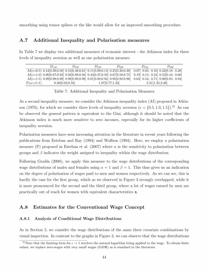
smoothing using tensor splines or the like would allow for an improved smoothing procedure.
A.7 Additional Inequality and Polarisation measures
In Table 7 we display two additional measures of economic interest - the Atkinson index for three
levels of inequality aversion as well as one polarisation measure.
D1M D1W D2M D2W D3M D3W
AI(ε=0.5) 0.44[0.39;0.50] 0.54[0.46;0.61] 0.11[0.09;0.14] 0.25[0.20;0.30] 0.07[ 0.05; 0.10] 0.22[0.18; 0.28]AI(ε=1.0) 0.90[0.87;0.93] 0.92[0.89;0.94] 0.43[0.37;0.50] 0.67[0.58;0.75] 0.19[ 0.15; 0.24] 0.52[0.44; 0.60]AI(ε=1.5) 0.99[0.98;0.99] 0.98[0.98;0.98] 0.91[0.88;0.94] 0.95[0.92;0.96] 0.63[ 0.54; 0.71] 0.90[0.85; 0.94]
P(α=β=1) 0.30[0.02;0.58] 1.07[0.77;1.33] 2.31[1.35;3.26]
Table 7: Additional Inequality and Polarisation Measures
As a second inequality measure, we consider the Atkinson inequality index (AI) proposed in Atkin-
son (1970), for which we consider three levels of inequality aversion (ε = {0.5, 1.0, 1.5}).21 As can
be observed the general pattern is equivalent to the Gini, although it should be noted that the
Atkinson index is much more sensitive to zero incomes, especially for its higher coefficients of
inequality aversion.
Polarisation measures have seen increasing attention in the literature in recent years following the
publications from Esteban and Ray (1994) and Wolfson (1994). Here, we employ a polarisation
measure (P) proposed in Esteban et al. (2007) where α is the sensitivity to polarisation between
groups and β indicates the weight assigned to inequality within the wage distribution.
Following Gradın (2000), we apply this measure to the wage distributions of the corresponding
wage distributions of males and females using α = 1 and β = 1. This thus gives us an indication
on the degree of polarisation of wages paid to men and women respectively. As we can see, this is
hardly the case for the first group, which as we observed in Figure 3 strongly overlapped, while it
is more pronounced for the second and the third group, where a lot of wages earned by men are
practically out of reach for women with equivalent characteristics x.
A.8 Estimates for the Conventional Wage Concept
A.8.1 Analysis of Conditional Wage Distributions
As in Section 5, we consider the wage distributions of the same three covariate combinations by
visual inspection. In contrast to the graphs in Figure 3, we can observe that the wage distributions
21Note that the limiting form for ε→ 1 involves the natural logarithm being applied to the wage. To obtain finitevalues, we replace zero-wages with very small wages (0.01e) as is standard in the literature.
44

of men and women overlap to a much greater degree, if one only considers the ordinary work-time
concept. Naturally, the wages are also a lot higher as the working time according to the introduced
concept is a superset of the conventional definition of working time.
D1.: 30 years, low education, no children, foreign, Mecklenburg−Western Pomerania
incs
Den
sity
Pro
babi
lity
of P
oint
Mas
s
0
0.05
0.1
0.15
0.2
0
0.1
0.2
0.3
0.4
0.5
0€/h 10€/h 20€/h 30€/h 40€/h 50€/h
femalemale
D2.: 40 years, median education, children, German, North Rhine−Westphalia
incs
Den
sity
Pro
babi
lity
of P
oint
Mas
s
0
0.05
0.1
0.15
0.2
0
0.1
0.2
0.3
0.4
0.5
0€/h 10€/h 20€/h 30€/h 40€/h 50€/h
femalemale
D3.: 50 years, high education, children, German, Bavaria
Den
sity
Pro
babi
lity
of P
oint
Mas
s
0
0.05
0.1
0.15
0.2
0
0.1
0.2
0.3
0.4
0.5
0€/h 10€/h 20€/h 30€/h 40€/h 50€/h
femalemale
Figure 6: Conditional wage distribution estimates of males (blue) and females (red).
For the first graph, we see that the graphs are again not adhering to the standard positive skew
normally found in most income related distributions. However, the skew is lower than in the case
in Figure 6. Nonetheless, also with these graphs it is observable that there are differences beyond
location and scale between the wage distribution of men and women.
This is also true for the second wage distribution, where women show a higher skewness as well as
a higher coefficient of variation. Additionally we can observe that women are much more likely to
be receiving no wages at all than men.
45

The third set of distributions displays a much wider distribution than originally. Especially for
women, we observe a much lower skewness, as for a lot of the women in this subgroup the working
time is significantly reduced if aspects like care work are not considered.
In Table 8 we display the equivalent measures to those displayed in Table 1 in the article.
D1m D1f D2m D2f D3m D3f
µ 3.95[ 3.23;4.85] 2.94[2.20;3.82] 14.62[13.23;15.97] 9.80[8.79;10.86] 29.01[26.05;32.39] 19.14[17.09;21.56]G(ρ=2) 0.24[ 0.18;0.31] 0.23[0.18;0.29] 0.18[ 0.15; 0.21] 0.24[0.21; 0.27] 0.23[ 0.20; 0.27] 0.30[ 0.26; 0.34]G(ρ=3) 0.79[ 0.74;0.83] 0.84[0.79;0.86] 0.38[ 0.34; 0.42] 0.56[0.49; 0.62] 0.35[ 0.30; 0.40] 0.48[ 0.44; 0.54]G(ρ=4) 0.84[ 0.82;0.86] 0.83[0.79;0.84] 0.47[ 0.42; 0.52] 0.67[0.60; 0.73] 0.41[ 0.36; 0.47] 0.57[ 0.52; 0.63]W(ρ=2) 3.00[ 2.33;3.74] 2.27[1.64;3.00] 12.01[10.85;13.17] 7.43[6.62; 8.31] 22.19[19.66;24.94] 13.45[11.84;15.18]W(ρ=3) 0.83[ 0.56;1.19] 0.49[0.31;0.78] 9.08[ 8.02;10.22] 4.36[3.38; 5.33] 18.92[16.53;21.47] 9.89[ 8.44;11.48]W(ρ=4) 0.63[ 0.48;0.84] 0.51[0.43;0.65] 7.78[ 6.74; 8.94] 3.28[2.40; 4.22] 17.07[14.69;19.51] 8.21[ 6.79; 9.69]
Table 8: Some distribution measures for 3 conditional wage distributions
The Table also shows that the expected wages are much higher both for men and women with
the discrepancy between wages of men and women generally reduced in contrast to the compre-
hensive wage definition used in the article. For the first group, it may even be noted that the
credible intervals for males and females overlap, although this is more likely down to the relatively
high uncertainty of the estimates in structured additive distributional regression than an actual
equivalence in the expected wages.
Concerning the Gini coefficient (G), we find generally find slightly reduced measures, although this
trend is not true for all six distributions and mostly non-significant.
Concerning the Equally Distributed Equivalent Earning (W), we find that it is generally higher
due to the higher expected income.
D1. D2. D3.
∆x for µ 0.74[0.53;1.04] 0.67[0.58;0.77] 0.66[0.56;0.78]∆x for W(ρ=2) 0.76[0.52;1.11] 0.62[0.53;0.72] 0.61[0.51;0.72]∆x for W(ρ=3) 0.59[0.33;1.09] 0.48[0.36;0.61] 0.52[0.42;0.64]∆x for W(ρ=4) 0.81[0.58;1.16] 0.42[0.30;0.57] 0.48[0.38;0.61]
Table 9: Ratios of male and female wage distribution measures
To get a measure of discrimination, we use the ratios between male and female wage measures,
as displayed in Table 9. As would be expected the measures decrease relative to the measures we
find in Table 2 using the comprehensive wage definition. Nonetheless, we still the same general
relationship that the EDEE induce a higher degree of discrimination than would be portrayed by
simple comparison of expected incomes.
Using the conventional concept, we also show the results if we aggregate the various subgroups:
46

µ W(ρ=2) W(ρ=3) W(ρ=4)∆a 0.69[0.66;0.72] 0.62[0.59;0.64] 0.47[0.45;0.50] 0.44[0.41;0.47]
Table 10: Average ratios of male and female wage distribution measures
Analogously to above, we find that although the magnitude is smaller, the general finding that
the inclusion of risk in the assessment of gender discrimination generally increases the magnitude
estimates is robust to the definition of work.
A.9 Estimates for other sub-populations
In Table 11, we display the ratio between female and male pay for two subgroups differentiated
by the region of residence, divided into the federal states belonging to former West Germany
(excluding Berlin) and former East Germany (including Berlin).
µconv0 µ0 µ W(ρ=2) W(ρ=3) W(ρ=4)
∆West 0.77[0.74;0.81] 0.57[0.53;0.63] 0.52[0.46;0.57] 0.47[0.42;0.52] 0.38[0.32;0.45] 0.36[0.30;0.42]∆East 0.87[0.80;0.93] 0.68[0.60;0.76] 0.68[0.60;0.76] 0.63[0.55;0.71] 0.62[0.52;0.73] 0.56[0.47;0.67]
Table 11: Average ratios of male and female wage distribution measures
Our findings echo those of the literature with the gender pay gap generally higher in the West
than in the East, regardless of the measure used. Again it should be noted that the discrepancy
is higher for the EDELER than for the conventional measure, both for the West and the East.
The same measure is displayed for a division along education levels. Here we solely differentiate in
a binary manner between those who have enjoyed higher education and those who have not. The
results are displayed in Table 12.
µconv0 µ0 µ W(ρ=2) W(ρ=3) W(ρ=4)
∆lower educ. 0.79[0.76;0.83] 0.59[0.54;0.65] 0.54[0.49;0.59] 0.49[0.45;0.55] 0.42[0.37;0.48] 0.39[0.35;0.45]∆higher educ. 0.76[0.72;0.80] 0.58[0.54;0.63] 0.53[0.49;0.58] 0.49[0.45;0.54] 0.41[0.37;0.47] 0.37[0.32;0.43]
Table 12: Average ratios of male and female wage distribution measures
Again we observe the same pattern of the measure increasing from left to right. Concerning the
difference between the two it is noteworthy that indeed there is very little discrepancy between
the two subgroups for any of the measures considered. While are more interactive differentiation
(especially including age) may show some ‘education effect’, a simple analysis with the other
variables integrated out, does not.
47

A.10 Misspecification Testing
A.10.1 Hypotheses and Algorithm
One quintessential assumption made for our estimation approach is the use of an adequate para-
metric form for the conditional wage distributions. This assumption is tested by considering the
following null-hypothesis H0 against the alternative hypothesis H1:
H0: The conditional wage distributions can be modelled by our parametric form, p(y | θ), for all
observed values of y and some values of θ derived for the corresponding covariates, x.
vs.
H1: The conditional wage distributions cannot be modelled by our parametric form, p(y | θ), for
all observed values of y and any values of θ derived for the corresponding covariates, x.
In order to test these hypotheses we will use an adaptation of the Kolmogorov-Smirnov test, which
is arguably the most renowned and most widely used test for distributional assumptions. Our
adaptation is based on the work of Andrews (1997) and Rothe and Wied (2013) who proposed a
frequentist framework for the testing of conditional distributions. Using the idea to transform the
conditional moment restrictions imposed by the parametric specification of our structured additive
distributional regression model into unconditional ones (see Rothe and Wied, 2013), we are able
to specify the test statistic Tn as
Tn =√n sup
(y,x)
| Hn(y,x)− H0n(y,x) |, (20)
where Hn(y,x) and H0n(y,x) constitute estimates of the joint cumulative distribution function of
both dependent and independent variable for n observations integrated up with respect to the
marginal distribution of the conditioning variables:
Hn(y,x) = n−1∑
1{Yi≤y}1{Xi≤x}
and
H0n(y,x) = n−1
∑Pn1{Xi≤x},
where Pn denotes the estimated cumulative density function based on n samples using structured
additive regression while 1 again denotes an indicator function.
As the asymptotic distribution of Tn under the null hypothesis depends on the data-generating
48

process in a complex fashion we use a bootstrap procedure to simulate it. In order to incorporate
the uncertainty attached to the parameter estimates we use draws from the MCMC realisations and
contrast it with simulated realisations of Y for a set of randomly selected covariate combinations
of X. Our bootstrap algorithm thus as follows:
Step 1 Draw a bootstrap sample of covariates {Xb,i; 1 ≤ i ≤ n} with replacement from the
obtained values in the sample {Xi; 1 ≤ i ≤ n}.
Step 2 Randomly select the m-th MCMC draw from set M for the parameter estimates,
yielding θ(m)b,1 (x), . . . , θ
(m)b,K (x).
Step 3 Use {θb,k(x); 1 ≤ k ≤ K} and {Xb,i; 1 ≤ i ≤ n} to simulate {Yb,i; 1 ≤ i ≤ n} in
accordance with the parametrically specified conditional distributions.
Step 4 Use bootstrapped data {Yb,i; 1 ≤ i ≤ n}, {Xb,i; 1 ≤ i ≤ n} and {θb,k(x); 1 ≤ k ≤ K} to
compute estimates Hb,n and H0b,n yielding the bootstrap realisation of the test statistic:
Tb,n =√n sup
(y,x)
| Hb,n(y,x)− H0b,n(y,x) |.
Using the simulated distribution of Tn we can then derive the corresponding p-value and or critical
values to assess the test statistic.
A.10.2 Use of MCMC samples for the misspecification test
To implement the test, we use 10,000 bootstrap draws from the algorithm discussed in Section
A.10.1. For our wage distributions have two independent MCMC samples, one for π0 and one for
a, b and c. Hence, we have a two dimensional sample set M = (1, . . . ,M1) × (1, . . . ,M2), with
M1 = M2 = 1000. A given random bootstrap sample b thus takes a random set of realisations
from the MCMC output {m1;m2} = m ∈M to yield πm1b , am2
b , bm2b and cm2
b .
A.10.3 Simulation study
We briefly assess the misspecification test from Section A.10.1 by means of three simple simulation
studies in order to validate its performance. In each simulation study, we consider a simple
framework with one explanatory variable which has a linear effect on all the predictors of the
Dagum distribution, i.e.
g(ηθk) = βθk0 + βθk1 x, (21)
where x is an integer from the interval [1, 10] and g is the log-link.
For the simulations we use 1,000 observations and 1000 bootstrap repetitions and contrast the
49

results for a true specification, as specified above, with a misspecified parametric model. For the
misspecification we use a log-normal distribution with mean and coefficient of variation equivalent
to that of the Dagum specification.
Sim. Study 1 Sim. Study 2 Sim. Study 3Sim.Run H0 TRUE H0FALSE H0 TRUE H0FALSE H0 TRUE H0FALSE
1 0.30 0.00 0.02 0.00 0.76 0.122 0.58 0.00 0.60 0.00 0.66 0.093 0.40 0.00 0.60 0.00 0.40 0.034 0.21 0.00 0.82 0.00 0.84 0.075 0.71 0.00 0.64 0.00 0.45 0.086 0.40 0.00 0.92 0.00 0.63 0.077 0.07 0.00 0.05 0.00 0.95 0.108 0.92 0.00 0.98 0.00 0.81 0.099 0.28 0.00 0.45 0.00 0.54 0.10
10 0.10 0.00 0.80 0.00 0.92 0.0811 0.91 0.00 0.57 0.00 0.62 0.0912 0.21 0.00 0.50 0.00 0.59 0.0913 0.47 0.00 0.00 0.00 0.90 0.0914 0.29 0.00 0.71 0.00 0.37 0.1215 0.66 0.00 0.15 0.00 0.72 0.1016 0.15 0.00 0.13 0.00 0.48 0.0917 0.92 0.00 0.15 0.00 0.48 0.1018 0.73 0.00 0.23 0.00 0.92 0.1219 0.49 0.00 0.41 0.00 0.46 0.1020 0.98 0.00 0.21 0.00 0.67 0.0921 0.06 0.00 0.31 0.00 0.80 0.0922 0.29 0.00 0.68 0.00 0.82 0.1023 0.26 0.00 0.73 0.00 0.84 0.1124 0.49 0.00 0.82 0.00 0.97 0.1025 0.39 0.00 0.57 0.00 0.57 0.1126 0.79 0.00 0.40 0.00 0.60 0.1127 0.91 0.00 0.06 0.00 0.80 0.1028 0.20 0.00 0.54 0.00 0.44 0.1029 0.35 0.00 0.92 0.00 0.56 0.0930 0.43 0.00 0.05 0.00 0.42 0.16µ 0.47 0.00 0.47 0.00 0.67 0.10σ 0.28 0.00 0.31 0.00 0.18 0.02Q1 0.26 0.00 0.17 0.00 0.50 0.09Q2 0.40 0.00 0.52 0.00 0.64 0.10Q3 0.70 0.00 0.70 0.00 0.82 0.10
Table 13: Results from Simulation Studies for Misspecificaiton Test
The result from our simulation studies are displayed in Table 13. The p-value for each simulation
run as well as the mean of the p-values of all simulation runs (µ), their standard deviation (σ) as
well as the three quartiles (Q1, Q2, Q3).
In the first two columns, we display the results for the a scenario where we have negligible parameter
uncertainty such that the standard deviation of the posterior distribution is 1% of its expectation.
As can be observed the p-values in the first column roughly follow a uniform distribution, as we
50

would expect, while the second column repeatedly rejects the null.
In the third and fourth column, we display a scenario with moderate parameter uncertainty such
that the standard deviation of the posterior distribution is 5% of its expectation. As for the first
two columns we see that the results are able to clearly distinguish between the correct and the
false specification.
In the last two columns, we assume considerable parameter uncertainty with the standard deviation
of the posterior distribution is 50% of its expectation. Given this large uncertainty, the model
specification test is less likely to reject the false hypothesis. With higher parameter uncertainty,
the test is thus conservative.
Overall, the simulation study indicates that the test generally works although its power is mitigated
by large parameter uncertainty.
A.11 Model Selection
Subsequently to asking whether one parametric model fits at all let us look at a handful of paramet-
ric models and consider their fit. Following our estimation approach we will consider the modelling
of the point mass for zero wages and positive wages separately. Here we will consider only one gen-
eric predictor for all parameters. While it would in theory be possible to specify the predictor for
each parameter individually, this would yield a high dimensional model selection problem, which
given the lack of automated routines is not feasible.
A.11.1 Variable selection for the logit model
For the logit model we simply consider three alternatives:
M01 As the first model, we use the model used in the paper.
M02 For comparison we will consider the model, using a linear approach to modelling the
impact of age, i.e. use a parabola (age + age2), with the other covariates specified as
before.
M03 Lastly, we will consider a model which only considers two education levels only differ-
entiating between those with and without university education.
For comparison of the models we will use the DIC, which has been shown to be an adequate model
selection criterion in Klein et al. (2015). The results are displayed in Table 14.
51

males femalesM0
1 301850 413997M0
2 337540 445537M0
3 336439 451336
Table 14: DIC for zero wages model approaches
A.11.2 Variable selection for the Dagum model
For the modelling of positive earnings we consider the the following five models:
M+1 As the first model, we use the model used in the paper.
M+2 For comparison we will consider a model, using a linear approach to modelling the
impact of age as above for all three parameters of the Dagum distribution.
M+3 Thirdly, we will consider a model, using only two education levels as above for all three
parameters of the Dagum distribution.
In contrast to the Dagum distribution we will also consider the log-normal distribution.
M+4 As a first log-normal specification, we will use the same specification as above for both
parameters of the log-normal.
M+5 As a first log-normal specification, we will use the same specification as above for µ,
while considering σ as a nuisance parameter and keeping it constant, as is standard in
the conventional literature.
The results are displayed in Table 15.
males females
M+1 22316.8 20687.2
M+2 23632.2 21864.9
M+3 23723.4 22946.8
M+4 24418.4 20931.5
M+5 24474.4 21239.3
Table 15: DIC for zero wages model approaches
52


