
THE FLORIDA STATE UNIVERSITY
FAMU-FSU COLLEGE OF ENGINEERING
A CONCENTRATED SOLAR THERMAL ENERGY SYSTEM
By
C. CHRISTOPHER NEWTON
A Thesis submitted to the Department of Mechanical Engineering
in partial fulfillment of the requirements for the degree of
Master of Science
Degree Awarded: Spring Semester, 2007

ii
The members of the Committee approve the Thesis of C. Christopher Newton defended on December 14, 2006.
Anjaneyulu Krothapalli
Professor Directing Thesis Patrick Hollis
Outside Committee Member Brenton Greska
Committee Member The Office of Graduate Studies has verified and approved the above named committee members.

iii
The dedication page is optional. You do not have to provide a dedication for your manuscript.

iv
ACKNOWLEDGEMENTS
The Acknowledgements page is also optional. You may use this section to express acknowledgement of those who have helped you with this manuscript and your academic career.
v
TABLE OF CONTENTS List of Tables ................................................................................................ Page viii List of Figures ................................................................................................ Page ix Abstract ...................................................................................................... Page xiv 1. Background ................................................................................................ Page 1 1.1 Introduction........................................................................................... Page 1 1.2 Historical Perspective of Solar Thermal Power and Process Heat ....... Page 2 1.2.1 Known Parabolic Dish Systems.......................................... Page 3 1.3 Solar Thermal Conversion .................................................................... Page 5 1.4 Solar Geometry (Fundamentals of Solar Radiation)............................. Page 6 1.4.1 Sun-Earth Geometric Relationship ..................................... Page 6 1.4.2 Angle of Declination........................................................... Page 7 1.4.3 Solar Time and Angles........................................................ Page 10 1.5 Solar Radiation ..................................................................................... Page 13 1.5.1 Extraterrestrial Solar Radiation .......................................... Page 13 1.5.2 Terrestrial Solar Radiation.................................................. Page 14 1.6 Radiative Properties .............................................................................. Page 17 1.7 Solar Collector/Concentrator ................................................................ Page 18 1.7.1 Acceptance Angle ............................................................... Page 21 1.7.2 Thermodynamic Limits of Concentration........................... Page 22 1.8 The Receiver/Absorber ......................................................................... Page 23 1.8.1 Cavity Receiver................................................................... Page 24 1.8.2 External Receiver................................................................ Page 25 1.9 Heat Storage.......................................................................................... Page 25 1.9.1 Sensible Heat Storage ......................................................... Page 25 1.9.2 Latent Heat Storage ............................................................ Page 26 1.10 Rankine Cycle..................................................................................... Page 26 1.10.1 Working Fluid................................................................... Page 29 1.10.2 Deviation of Actual Cycle from Ideal............................... Page 29 1.11 Steam Turbine..................................................................................... Page 30 1.11.1 Impulse Turbine ................................................................ Page 31 1.11.2 Reaction Turbine............................................................... Page 31 1.11.3 Turbine Efficiency ............................................................ Page 32 1.12 Overview............................................................................................. Page 33 2. Experimental Apparatus and Procedures ........................................................ Page 34 2.1 Introduction........................................................................................... Page 34 2.2 Solar Collector ...................................................................................... Page 34 2.3 The Receiver ......................................................................................... Page 36 2.4 Steam Turbine....................................................................................... Page 39

vi
2.5 Gear-Train............................................................................................. Page 41 2.6 Working Fluid of Solar Thermal System.............................................. Page 43 2.7 Feed-Water Pump ................................................................................. Page 44 2.8 Tracking ............................................................................................... Page 45 2.9 Data Acquisition ................................................................................... Page 49 2.9.1 Instrumentation ................................................................... Page 50 2.10 Power Supply ...................................................................................... Page 50 2.11 Generator/Alternator ........................................................................... Page 53 3. Analysis/Results and Discussion .................................................................... Page 55 3.1 Introduction........................................................................................... Page 55 3.2 Solar Calculations ................................................................................. Page 55 3.3 Analysis of the Dish.............................................................................. Page 57 3.3.1 Efficiency of Collector........................................................ Page 61 3.4 Receiver ............................................................................................... Page 66 3.4.1 Boiler Efficiency................................................................. Page 76 3.5 Turbine Efficiency ................................................................................ Page 77 3.6 Turbine/Gear-Train Analysis ................................................................ Page 78 3.7 Analysis of the Rankine Cycle.............................................................. Page 79 3.8 Generator and Energy Conversion Efficiency ...................................... Page 81 4. Conclusions …................................................................................................ Page 83 4.1 Introduction........................................................................................... Page 83 4.2 Solar Calculations ................................................................................. Page 83 4.3 Trackers ............................................................................................... Page 83 4.4 Solar Concentrator ................................................................................ Page 84 4.5 Receiver/Boiler ..................................................................................... Page 84 4.6 Steam Turbine....................................................................................... Page 85 4.7 Generator .............................................................................................. Page 85 4.8 Cycle Conclusions ............................................................................... Page 85 4.9 Future Work ......................................................................................... Page 86 APPENDICES ................................................................................................ Page 88 A Rabl’s Theorem..................................................................................... Page 88 B Solar Angle and Insolation Calculations .............................................. Page 91 C Solar Calculations for October 12th ..................................................... Page 100 D Collector Efficiency for Varied Wind Speeds ...................................... Page 105 E Calculations for Collector Efficiency on Oct. 12th for Beam Insolation Page 111 F Collector Efficiency as Receiver Temperature Increases ..................... Page 118 G Geometric Concentration Ration and Maximum Theoretical Temperature Page 121 H Geometric Concentration Ratio as Function of Receiver Temperature Page 125 I Receiver/Boiler Efficiency Calculations .............................................. Page 128 J Mass Flow Rate Calculations for Steam into Turbine.......................... Page 129 K Steam Turbine Efficiency Calculations ................................................ Page 131

vii
L Rankine Cycle Calculations.................................................................. Page 134 M Drawings/Dimensions of T-500 Impulse Steam Turbine and Gear-Train Page 142 N Receiver Detailed Drawings and Images.............................................. Page 147 O Solar Charger Controller Electrical Diagram ....................................... Page 157 P Windstream Power Low RPM Permanent Magnet DC Generator ....... Page 159 REFERENCES ................................................................................................ Page # BIOGRAPHICAL SKETCH .............................................................................. Page #

viii
LIST OF TABLES Table 1.1: Average values of atmospheric optical depth (k) and sky diffuse factor (C) for average atmospheric conditions at sea level for the United States Page 16 Table 1.2: Specular Reflectance Values for Different Reflector Materials......... Page 18 Table 2.1: Design Conditions of the T-500 Impulse Turbine.............................. Page 39 Table 2.2: Correlation of Pump Speed to Flow Rate ........................................... Page 45 Table 3.1: Test results for mechanical power determination of steam turbine/ gear-train output shaft ........................................................................ Page 79 Table 3.2: Inlet and outlet temperature, pressure, and entropy values for the various components of the system. .................................................... Page 80 Table 3.3: Sample of loads tested on generator and the resulting voltage and power Page 45
ix
LIST OF FIGURES Figure 1.1: Solar Furnace used by Lavoisier ...................................................... Page 2 Figure 1.2: Parabolic collector powered printing press ...................................... Page 3 Figure 1.3: Photographs of Vanguard and McDonell Douglas concentrator systems Page 5 Figure 1.4: Motion of the earth about the sun ..................................................... Page 7 Figure 1.5: Declination Angle as a Function of the Date ................................... Page 8 Figure 1.6: The Declination Angle ..................................................................... Page 8 Figure 1.7: Equation of Time as a function of the time of year .......................... Page 11 Figure 1.8: Length of Day as a function of the time of year ............................... Page 12 Figure 1.9: The Variation of Extraterrestrial Radiation with time of year ......... Page 14 Figure 1.10: Variance of the Total Insolation compared to Beam Insolation...... Page 17 Figure 1.11: Concentration by parabolic concentrating reflector for a beam parallel to the axis of symmetry, and at an angle to the axis ...................... Page 19 Figure 1.12: Cavity Type Receiver ..................................................................... Page 24 Figure 1.13: Basic Rankine Power Cycle ........................................................... Page 26 Figure 1.14: T-s Diagram of Ideal and Actual Rankine Cycle ............................ Page 27 Figure 1.15: T-s Diagram showing effect of losses between the boiler and turbine Page 30 Figure 1.16: Diagram showing difference between an impulse and a reaction turbine Page 31 Figure 2.1: Image of dish sections and assembled dish ...................................... Page 35 Figure 2.2: Image of applying aluminized mylar to surface of dish ................... Page 35 Figure 2.3: Exploded 3-D layout of receiver ...................................................... Page 36 Figure 2.4: Image of Draw-salt mixture in receiver ........................................... Page 37 Figure 2.5: Diagram of instrumentation of receiver ........................................... Page 38 Figure 2.6: Image of receiver assembled at focal region of concentrator ........... Page 38
x
Figure 2.7: Images of T-500 Impulse Turbine Rotor .......................................... Page 39 Figure 2.8: Images of T-500 Steam Turbine housing ......................................... Page 40 Figure 2.9: Images of T-500 Steam Turbine Assembled .................................... Page 40 Figure 2.10: Images of Gear-Train Assembly .................................................... Page 42 Figure 2.11: Images of Steam Turbine and Gear-Train Assembled ................... Page 42 Figure 2.12: Image of water tank ........................................................................ Page 43 Figure 2.13: Image of pump and controller ........................................................ Page 44 Figure 2.14: Images of the frame with actuators ................................................ Page 46 Figure 2.15: Image of LED3 Solar Tracker Module .......................................... Page 47 Figure 2.16: Image of LED3 module in plexi-glass housing .............................. Page 47 Figure 2.17: Image of LED3 module sealed in plexi-glass housing ................... Page 48 Figure 2.18: Image of tracking module attached to concentrator ....................... Page 48 Figure 2.19: Image of the data acquisition program used (SURYA) ................. Page 49 Figure 2.20: Two 12-volt deep cycle batteries wired in series ............................ Page 51 Figure 2.21: Thin-filmed flexible photovoltaics.................................................. Page 51 Figure 2.22: Image of Solar Charger Controller.................................................. Page 52 Figure 2.23: Image of 400 Watt DC to AC Power Inverter................................. Page 53 Figure 2.24: Image of Windstream Power 10 AMP Permanent Magnet Generator Page 53 Figure 2.25: Performance Curves for the Generator............................................ Page 54 Figure 2.26: Image Generator, Gear-train, and Steam Turbine Assembled ........ Page 54 Figure 3.1: Solar Altitude and Azimuth Angles for October 12th ...................... Page 56 Figure 3.2: Plot showing comparison between available Total Insolation and available Beam Insolation ............................................................... Page 57 Figure 3.3: Relationship between the concentration ratio and the receiver operation temperature ....................................................................... Page 61

xi
Figure 3.4: Heat loss from receiver as a function of the receiver temperature.... Page 65 Figure 3.5: Experimental collector efficiency over range of values.................... Page 66 Figure 3.6: Transient Cooling of Thermal Bath at Room Temperature ............. Page 67 Figure 3.7: Temperature Profile for Steady-Flow Tests of 1.0 LPM .................. Page 69 Figure 3.8: Useable Thermal Energy from Steady-Flow Tests of 1.0 LPM........ Page 69 Figure 3.9: Various Flow-Rate Tests for Steam Flashing ................................... Page 71 Figure 3.10: Temperature and Pressure Profile for Flash Steam with Feed-Water at a Flow-Rate of 0.734 LPM ......................................................... Page 71 Figure 3.11: Temperature and Pressure Profile for Flash Steam with Feed-Water at a Flow-Rate of 1.36 LPM (test 1) .............................................. Page 72 Figure 3.12: Temperature and Pressure Profile for Flash Steam with Feed-Water at a Flow-Rate of 1.36 LPM (test 2) ............................................... Page 72 Figure 3.13: Plot of Temperature Profiles for Thermal Bath, Receiver Inlet, Receiver Exit, Turbine Inlet, Turbine Exit, and Feed-Water on October 12th ..................................................................................... Page 74 Figure 3.14: Initial Heating of System from Ambient to 700 K.......................... Page 74 Figure 3.15: Run one of multiple tests performed on October 12th .................... Page 75 Figure 3.16: Available Thermal Energy from System on October 12th test ........ Page 76 Figure 3.17: T-s Diagram for the Concentrated Solar Thermal System.............. Page 80 Figure A.1: Radiation transfer from source through aperture to receiver .......... Page 88 Figure B.1: Declination Angle as a function of date ........................................... Page 91 Figure B.2: Equation of time as a function of date ............................................. Page 93 Figure B.3: Length of day as a function of date ................................................. Page 94 Figure B.4: Variance of angle of incidence as a function of date ....................... Page 95 Figure B.5: Variation of extraterrestrial solar radiation as function of date ....... Page 97 Figure B.6: Variation of extraterrestrial radiation to the nominal solar constant Page 97

xii
Figure B.7: Total insolation compared to the beam insolation ........................... Page 99 Figure D.1: Heat loss from receiver for wind speeds less than 0.339 m/s .......... Page 107 Figure D.2: Heat loss from receiver for wind speeds greater than 0.339 m/s .... Page 107 Figure D.3: Thermal energy produced by collector for winds less than 0.339 m/s Page 109 Figure D.4: Thermal energy produced by collector for winds greater than 0.339 m/s Page 109 Figure D.5: Collector efficiency for wind speeds less than 0.339 m/s ............... Page 110 Figure D.6: Collector efficiency for wind speeds greater than 0.339 m/s .......... Page 110 Figure E.1: Solar altitude and azimuth angles for October 12th ........................ Page 112 Figure E.2: Angle of incidence for October 12th ............................................... Page 113 Figure E.3: Beam insolation incident on collector for October 12th .................. Page 115 Figure E.4: Varied collector efficiency for October 12th ................................... Page 117 Figure F.1: Heat loss from receiver as temperature increases ............................ Page 119 Figure F.2: Collector performance as receiver temperature increases ................ Page 120 Figure H.1: Concentration Ratio as a function of temperature ........................... Page 127 Figure M.1: Detailed drawing of complete assembly of turbine and gear-train . Page 143 Figure M.2: Detailed drawing of turbine rotor blades ........................................ Page 144 Figure M.3: Detailed drawing of first stage for gear-train ................................. Page 145 Figure M.4: Detailed drawing of third bearing plate of gear-train ..................... Page 146 Figure N.1: Dimensioned diagram of receiver cap ............................................. Page 148 Figure N.2: Dimensioned diagram of main receiver housing ............................. Page 149 Figure N.3: Dimensioned diagram of receiver outer coils .................................. Page 150 Figure N.4: Dimensioned diagram of receiver inner coils .................................. Page 151 Figure N.5: Dimensioned diagram of receiver water drum ................................ Page 152 Figure N.6: 3-D CAD images of receiver ........................................................... Page 153

xiii
Figure N.7: Image of receiver cap, water drum, and coils assembled ................ Page 153 Figure N.8: Images of receiver main housing ..................................................... Page 154 Figure N.9: Image of receiver assembled .......................................................... Page 154 Figure N.10: Image for receiver fully assembled and feed tubes installed ......... Page 155 Figure N.11: Images of receiver instrumented at focal region of concentrator .. Page 155 Figure N.12: Image of receiver being subjected to concentrated solar radiation Page 156 Figure O.1: Diagram of solar charger controller circuit board ........................... Page 157 Figure O.2: Schematic of solar charger controller .............................................. Page 158 Figure P.1: Diagram, specs, and performance curves of generator .................... Page 160
xiv
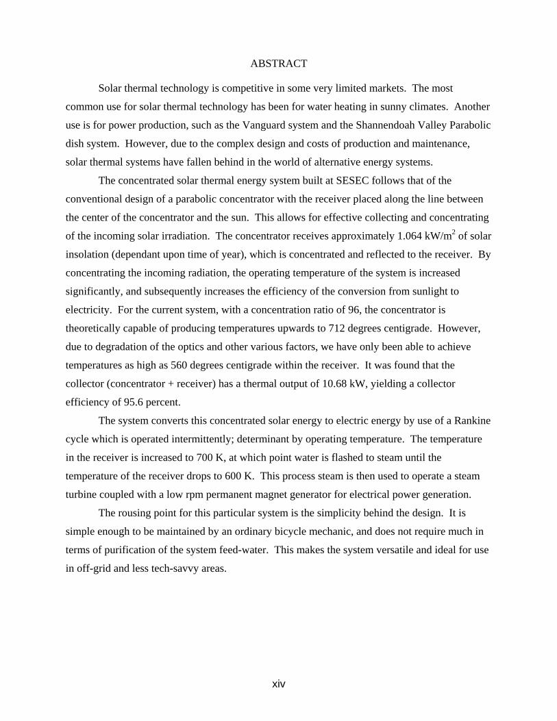
ABSTRACT
Solar thermal technology is competitive in some very limited markets. The most
common use for solar thermal technology has been for water heating in sunny climates. Another
use is for power production, such as the Vanguard system and the Shannendoah Valley Parabolic
dish system. However, due to the complex design and costs of production and maintenance,
solar thermal systems have fallen behind in the world of alternative energy systems.
The concentrated solar thermal energy system built at SESEC follows that of the
conventional design of a parabolic concentrator with the receiver placed along the line between
the center of the concentrator and the sun. This allows for effective collecting and concentrating
of the incoming solar irradiation. The concentrator receives approximately 1.064 kW/m2 of solar
insolation (dependant upon time of year), which is concentrated and reflected to the receiver. By
concentrating the incoming radiation, the operating temperature of the system is increased
significantly, and subsequently increases the efficiency of the conversion from sunlight to
electricity. For the current system, with a concentration ratio of 96, the concentrator is
theoretically capable of producing temperatures upwards to 712 degrees centigrade. However,
due to degradation of the optics and other various factors, we have only been able to achieve
temperatures as high as 560 degrees centigrade within the receiver. It was found that the
collector (concentrator + receiver) has a thermal output of 10.68 kW, yielding a collector
efficiency of 95.6 percent.
The system converts this concentrated solar energy to electric energy by use of a Rankine
cycle which is operated intermittently; determinant by operating temperature. The temperature
in the receiver is increased to 700 K, at which point water is flashed to steam until the
temperature of the receiver drops to 600 K. This process steam is then used to operate a steam
turbine coupled with a low rpm permanent magnet generator for electrical power generation.
The rousing point for this particular system is the simplicity behind the design. It is
simple enough to be maintained by an ordinary bicycle mechanic, and does not require much in
terms of purification of the system feed-water. This makes the system versatile and ideal for use
in off-grid and less tech-savvy areas.
1
CHAPTER 1
BACKGROUND
1.1 Introduction
Even in today’s world market, with all of the vast technology advancements and
improvements, there are still people who live in darkness at night and use candle light or
kerosene lamps to study. These people have the knowledge that electricity exists;
however, the area in which they reside lacks the infrastructure and resources for such an
amenity. Also, throughout the world, the demand for useable energy is increasing
rapidly, with electricity being the energy of choice. This electricity production,
however, does not come free. There is cost associated with the infrastructure for setting
up new power production facilities and the rising cost and lack of natural resources such
as oil, coal, and natural gas. One solution is to steer away from conventional methods
and look for novel, alternative, renewable, energy resources, such as solar energy.
The sun is an excellent source of radiant energy, and is the world’s most abundant
source of energy. It emits electromagnetic radiation with an average irradiance of 1353
W/m21 on the earth’s surface (Goswami, Duffie). The solar radiation incident on the
Earth’s surface is comprised of two types of radiation – beam and diffuse, ranging in the
wavelengths from the ultraviolet to the infrared (300 to 200 nm), which is characterized
by an average solar surface temperature of approximately 6000°K (Rapp). The amount
of this solar energy that is intercepted is 5000 times greater than the sum of all other
inputs – terrestrial nuclear, geothermal and gravitational energies, and lunar gravitational
energy (Goswami). To put this into perspective, if the energy produced by 25 acres of
the surface of the sun were harvested, there would be enough energy to supply the current
energy demand of the world.
1 The average amount of solar radiation falling on a surface normal to the rays of the sun outside the atmosphere of the earth at mean earth-sun distance, as measured by NASA (Goswami).
2
When dealing with solar energy, there are two basic choices. The first is
photovoltaics, which is direct energy conversion that converts solar radiation to
electricity. The second is solar thermal, in which the solar radiation is used to provide
heat to a thermodynamic system, thus creating mechanical energy that can be converted
to electricity. In commercially available photovoltaic systems, efficiencies are on the
order of 10 to 15 percent, where in a solar thermal system, efficiencies as high as 30
percent are achievable (Powerfromthesun). This work focuses on the electric power
generation of a parabolic concentrating solar thermal system.
1.2 Historical Perspective of Solar Thermal Power and Process Heat
Records date as far back as 1774 for attempts to harness the sun’s energy for
power production. The first documented attempt is that of the French chemist Lavoisier
and the English scientist Joseph Priestley when they developed the theory of combustion
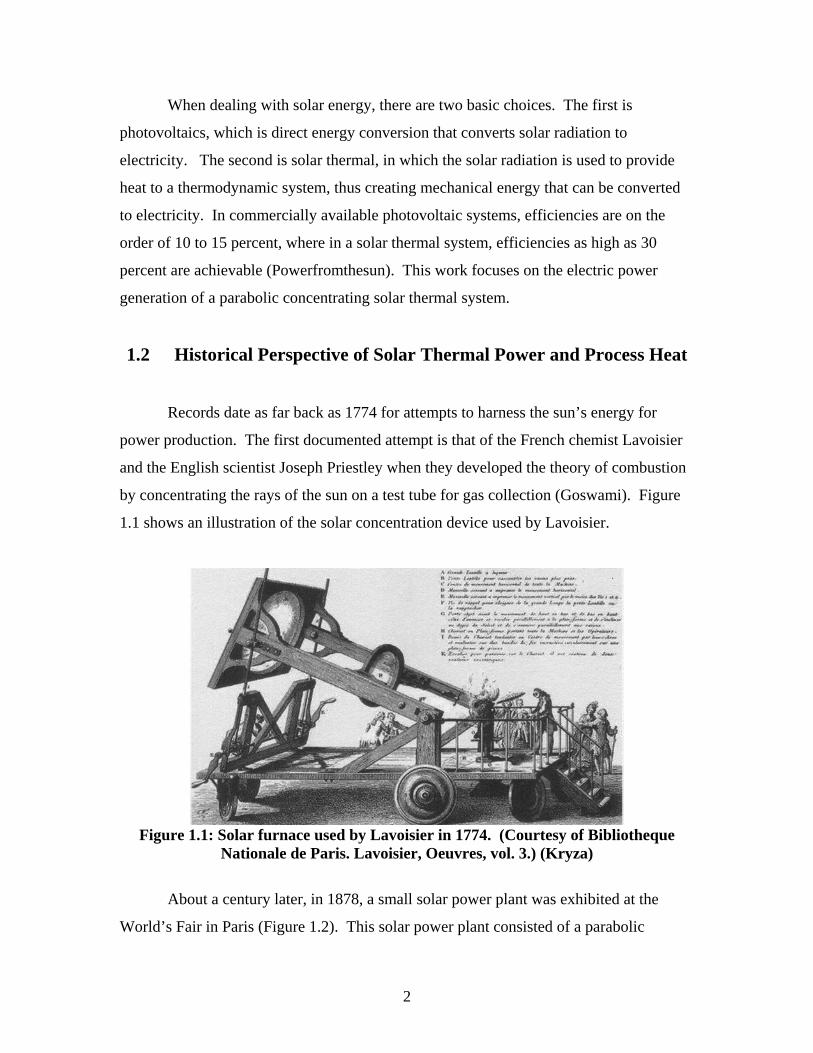
by concentrating the rays of the sun on a test tube for gas collection (Goswami). Figure
1.1 shows an illustration of the solar concentration device used by Lavoisier.
Figure 1.1: Solar furnace used by Lavoisier in 1774. (Courtesy of Bibliotheque
Nationale de Paris. Lavoisier, Oeuvres, vol. 3.) (Kryza)
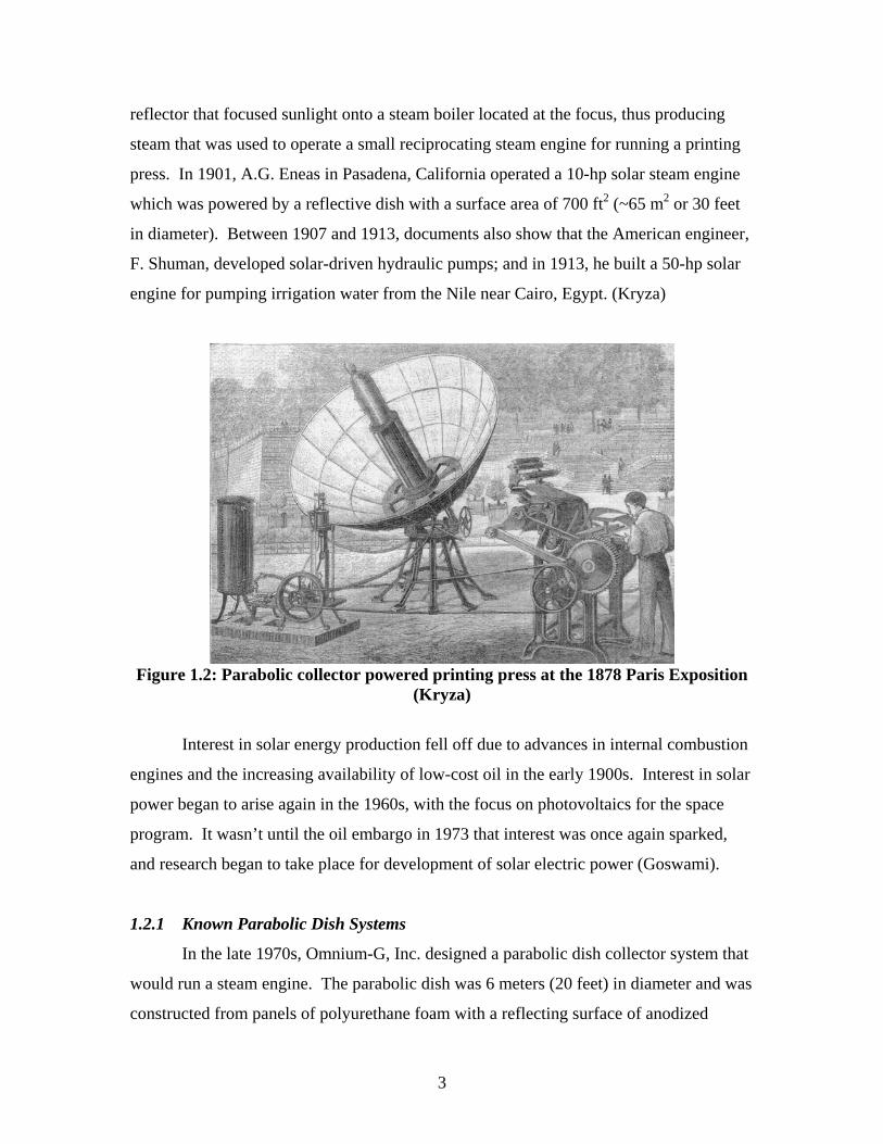
About a century later, in 1878, a small solar power plant was exhibited at the
World’s Fair in Paris (Figure 1.2). This solar power plant consisted of a parabolic
3
reflector that focused sunlight onto a steam boiler located at the focus, thus producing
steam that was used to operate a small reciprocating steam engine for running a printing
press. In 1901, A.G. Eneas in Pasadena, California operated a 10-hp solar steam engine
which was powered by a reflective dish with a surface area of 700 ft2 (~65 m2 or 30 feet
in diameter). Between 1907 and 1913, documents also show that the American engineer,
F. Shuman, developed solar-driven hydraulic pumps; and in 1913, he built a 50-hp solar
engine for pumping irrigation water from the Nile near Cairo, Egypt. (Kryza)
Figure 1.2: Parabolic collector powered printing press at the 1878 Paris Exposition
(Kryza)
Interest in solar energy production fell off due to advances in internal combustion
engines and the increasing availability of low-cost oil in the early 1900s. Interest in solar
power began to arise again in the 1960s, with the focus on photovoltaics for the space
program. It wasn’t until the oil embargo in 1973 that interest was once again sparked,
and research began to take place for development of solar electric power (Goswami).
1.2.1 Known Parabolic Dish Systems
In the late 1970s, Omnium-G, Inc. designed a parabolic dish collector system that
would run a steam engine. The parabolic dish was 6 meters (20 feet) in diameter and was
constructed from panels of polyurethane foam with a reflecting surface of anodized
4
aluminum (Stine). The receiver for the system was of the cavity type and used a single
coil of stainless steel tubing buried in molten aluminum inside of an Inconel housing.
The aluminum was used as a type of latent heat storage and to provide uniform heat
distribution and thermal storage once melted. The aperture of the receiver was 200mm (8
inches) in diameter, thus giving a geometric concentration ratio of 900. A double-acting
reciprocating two cylinder 34 kW (45 hp) steam engine was used with the system,
however, it was found to be oversized and operated at 1000 rpm with steam at 315°C and
2.5 MPa (350 psia). One main issue with this particular parabolic dish collector system
was that it had a very low reflectance and a large optical error, thus it supplied less
energy at the focal region than was needed to power the steam engine.
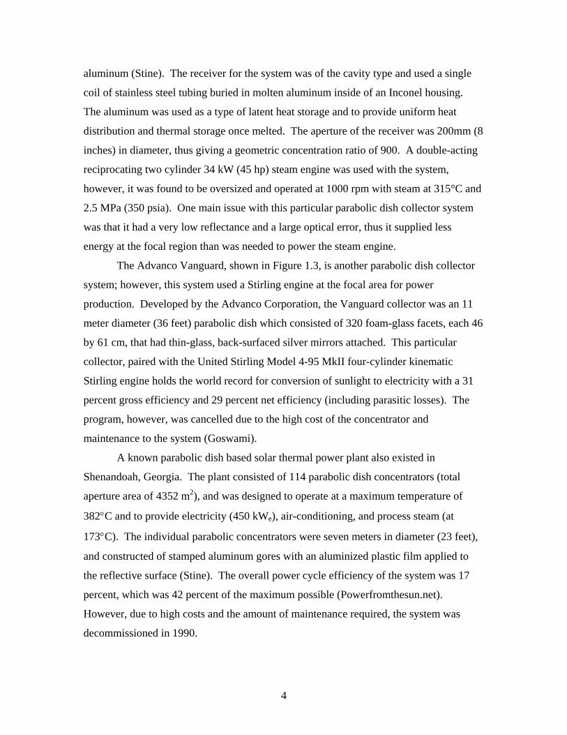
The Advanco Vanguard, shown in Figure 1.3, is another parabolic dish collector
system; however, this system used a Stirling engine at the focal area for power
production. Developed by the Advanco Corporation, the Vanguard collector was an 11
meter diameter (36 feet) parabolic dish which consisted of 320 foam-glass facets, each 46
by 61 cm, that had thin-glass, back-surfaced silver mirrors attached. This particular
collector, paired with the United Stirling Model 4-95 MkII four-cylinder kinematic
Stirling engine holds the world record for conversion of sunlight to electricity with a 31
percent gross efficiency and 29 percent net efficiency (including parasitic losses). The
program, however, was cancelled due to the high cost of the concentrator and
maintenance to the system (Goswami).
A known parabolic dish based solar thermal power plant also existed in
Shenandoah, Georgia. The plant consisted of 114 parabolic dish concentrators (total
aperture area of 4352 m2), and was designed to operate at a maximum temperature of
382°C and to provide electricity (450 kWe), air-conditioning, and process steam (at
173°C). The individual parabolic concentrators were seven meters in diameter (23 feet),
and constructed of stamped aluminum gores with an aluminized plastic film applied to
the reflective surface (Stine). The overall power cycle efficiency of the system was 17
percent, which was 42 percent of the maximum possible (Powerfromthesun.net).
However, due to high costs and the amount of maintenance required, the system was
decommissioned in 1990.

5
Figure 1.3: Photographs of the Vanguard (left) and McDonnell Douglas (right)
parabolic concentrator systems.
Other known parabolic concentrator systems, such as Solarplant One, McDonnell
Douglas Stirling Systems (Figure 1.3), Power Kinetics, Inc. Captiol Concrete Collector,
the Jet Propulsion Laboratories Test-Bed Concentrators, and a few other projects in
conjunction with Sandia National Laboratories, have been designed and tested in the last
twenty years. In the early 1990s, Cummins Engine Company attempted to commercialize
a dish-stirling system by teaming up with SunLab, but this company pulled out in 1996 to
focus solely on its core diesel-engine business. It appears that Sandia National
Laboratories is still currently researching new systems. The apparent downfall for the
majority of the solar thermal systems mentioned here is due to the extremely high cost
and high maintenance of the systems.
1.3 Solar Thermal Conversion
The basic principle of solar thermal collection is that when solar radiation is
incident on a surface (such as that of a black-body), part of this radiation is absorbed, thus
increasing the temperature of the surface. As the temperature of the body increases, the
surface loses heat at an increasing rate to the surroundings. Steady-state is reached when
the rate of the solar heat gain is balanced by the rate of heat loss to the ambient
surroundings. Two types of systems can be used to utilize this solar thermal conversion:
6
passive systems and active systems (Duffie). For our purposes, an active system is
utilized, in which an external solar collector with a heat transfer fluid is used to convey
the collected heat. The chosen system for the solar thermal conversion at SESEC is that
of the parabolic concentrator type.
1.4 Solar Geometry (Fundamentals of Solar Radiation)
In order to track the sun throughout the day for every day of the year, there are
geometric relationships that need to be known to find out where to position the collector
with respect to the time. In order to perform these calculations, a few facts about the sun
need be known.
The sun is considered to be a sphere km5109.13 × in diameter. The surface of the sun is
approximated to be equivalent to that of a black body at a temperature of 6000K with an
energy emission rate of kW23108.3 × . Of this amount of energy, the earth intercepts
only a small amount, approximately kW14107.1 × , of which 30 percent is reflected to
space, 47 percent is converted to low-temperature heat and reradiated to space, and 23
percent powers the evaporation/precipitation cycle of the biosphere (Goswami).
1.4.1 Sun-Earth Geometric Relationship
The earth makes one rotation about its axis every 24 hours and completes a
rotation about the sun in approximately 365 ¼ days. The path the earth takes around the
sun is located slightly off center, thus making the earth closest to the sun at the winter
solstice (Perihelion), at m1110471.1 × , and furthest from the sun at the summer solstice
(Aphelion), at a distance of m1110521.1 × , when located in the northern hemisphere
(Goswami) (Powerfromthesun.net)(Duffie). During Perihelion, the earth is about 3.3
percent closer, and the solar intensity is proportional to the inverse square of the distance,
thus making the solar intensity on December 21st about 7 percent higher than that on
June 21st (Rapp). The axis of rotation of the earth is tilted at an angle of 23.45° with
respect to its orbital plane, as shown in Figure 1.4. This tilt remains fixed and is the
cause for the seasons throughout the year.

7
Figure 1.4: Motion of the earth about the sun.
1.4.2 Angle of Declination
The earth’s equator is considered to be in the equatorial plane. By drawing a line
between the center of the earth and the sun, as shown in Figure 1.6 the angle of
declination, δs, is derived. The declination varies between -23.45° on December 21 to
+23.45° on June 21. Stated simply, the declination has the same numerical value as the
latitude at which the sun is directly overhead at solar noon on a given day, where the
extremes are the tropics of Cancer (23.45° N) and Capricorn (23.45° S). The angle of
declination, δs, is estimated by use of the following equation, or the resultant graph in
Figure 1.5:
⎥⎥⎦
⎤
⎢⎢⎣
⎡⎟⎠⎞
⎜⎝⎛ +
⋅=o
o
365284360sin45.23 n
sδ (1-1)
where n is the day number during the year with the first of January set as n = 1
(Goswami, Duffie).

8
1 51 101 151 201 251 301 351
30
10
10
30
Julian Date (1 to 365)
Ang
le o
f Dec
linat
ion
(Deg
)
Figure 1.5: Declination Angle as a Function of the Date.
Figure 1.6: The declination angle (shown in the summer
solstice position where δ = +23.45°)
9
In order to simplify calculations, it will be assumed that the earth is fixed and the
sun’s apparent motion be described in a coordinate system fixed to the earth with the
origin being at the site of interest, which for this work is Tallahassee, FL at Latitude
30.38° North and Longitude 84.37° West. By assuming this type of coordinate system, it
allows for the position of the sun to be described at any time by the altitude and azimuth
angles. The altitude angle, α, is the angle between a line collinear with the sun’s rays and
the horizontal plane, and the azimuth angle, αs, is the angle between a due south line and
the projection of the site to the sun line on the horizontal plane. For the azimuth angle,
the sign convention used is positive if west of south and negative if east of south. The
angle between the site to sun line and vertical at site is the zenith angle, z, which is found
by subtracting the altitude angle from ninety degrees:
α−= o90z (1-2)
However, the altitude and azimuth angles are not fundamental angles and must be related
to the fundamental angular quantities of hour angle (hs), latitude (L), and declination
(δs). The hour angle is based on the nominal time requirement of 24 hours for the sun to
move 360° around the earth, or 15° per hour, basing solar noon (12:00) as the time that
the sun is exactly due south (Powerfromthesun.net). The hour angle, hs, is defined as:
( )degreemin/4
noonsolar local from minutesnoonsolar from hours15 =⋅= osh (1-3)
The same rules for sign convention for the azimuth angle are applied for the values
obtained for the hour angle, that is, the values east of due south (morning) are negative;
and the values west of due south (afternoon) are positive. The latitude angle, L, is
defined as the angle between the line from the center of the earth to the site of interest
and the equatorial plane; and can easily found on an atlas or by use of the Global
Positioning System (GPS).

10
1.4.3 Solar Time and Angles
By using the previously defined angles, the solar time and resulting solar angles
can be defined. Solar time is used in predicting the direction of the sun’s rays relative to
a particular position on the earth. Solar time is location (longitude) dependent, and is
nominally different from that of the local standard time for the area of interest. The
relationship between the local solar time and the local standard time (LST) is:
degreemin/4)(TimeSolar ⋅−++= localst llETLST (1-4)
where ET is the equation of time, a correction factor that accounts for the irregularity of
the speed of the earth’s motion around the sun, lst is the standard time meridian, and llocal
is the local longitude. The equation of time is calculated by use of the following
empirical equation:
)sin(5.1)cos(53.7)2sin(87.9minutes)(in BBBET −−= (1-5)
Where B, in degrees, is defined as:
36481360 −
⋅=nB o (1-6)
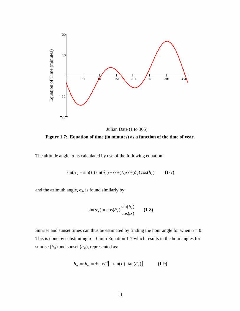
The equation of time can also be estimated from Figure 1.7, in which Equation 1-5 is
plotted to the time of year.
11
1 51 101 151 201 251 301 351
20
10
10
20
Julian Date (1 to 365)
Equa
tion
of T
ime
(min
utes
)
Figure 1.7: Equation of time (in minutes) as a function of the time of year.
The altitude angle, α, is calculated by use of the following equation:
)cos()cos()cos()sin()sin()sin( sss hLL δδα += (1-7)
and the azimuth angle, αs, is found similarly by:
)cos()sin(
)cos()sin(α
δα sss
h= (1-8)
Sunrise and sunset times can thus be estimated by finding the hour angle for when α = 0.
This is done by substituting α = 0 into Equation 1-7 which results in the hour angles for
sunrise (hsr) and sunset (hss), represented as:
[ ])tan()tan(cosor 1ssrss Lhh δ⋅−±= − (1-9)

12
The sunrise and sunset times are dependent on the day of the year, with the longest day
being the summer solstice. The hour angle also corresponds to the time from solar noon
with the hour angle changing at a rate of 15 degrees per hour. Thus the length of of the
days can be estimated by use of Equation 1-10, yielding Figure 1.8.
hour
srss hhdeg15
LengthDay +
= (1-10)
However, to the eye it may appear that the calculated times are off by several minutes as
to when the sun actually rises and sets. This is due to the observers’ line of sight and
their interpretation of sunrise and sunset. By convention, the times are solved for when
the center of the sun is at the horizon.
1 51 101 151 201 251 301 35110
11
12
13
14
Julian Date (1 to 365)
Leng
th o
f Day
(hou
rs)
Figure 1.8: Length of day, in hours, as a function of the date.
13
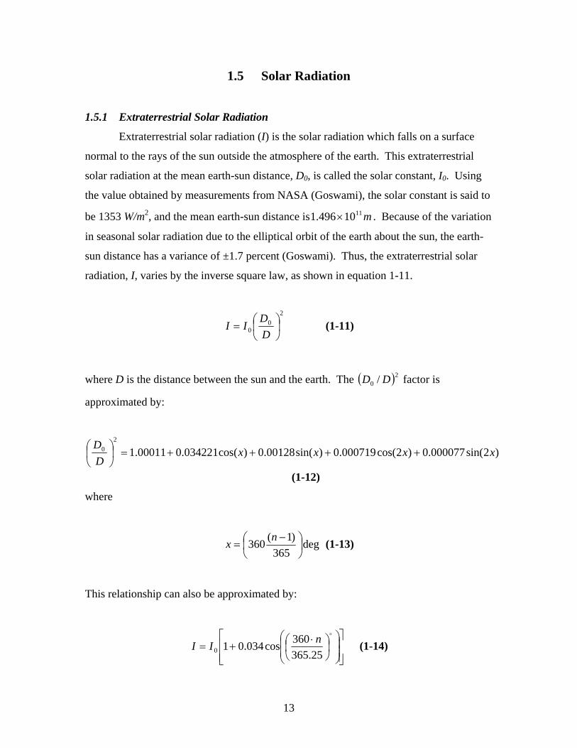
1.5 Solar Radiation
1.5.1 Extraterrestrial Solar Radiation
Extraterrestrial solar radiation (I) is the solar radiation which falls on a surface
normal to the rays of the sun outside the atmosphere of the earth. This extraterrestrial
solar radiation at the mean earth-sun distance, D0, is called the solar constant, I0. Using
the value obtained by measurements from NASA (Goswami), the solar constant is said to
be 1353 W/m2, and the mean earth-sun distance is m1110496.1 × . Because of the variation
in seasonal solar radiation due to the elliptical orbit of the earth about the sun, the earth-
sun distance has a variance of ±1.7 percent (Goswami). Thus, the extraterrestrial solar
radiation, I, varies by the inverse square law, as shown in equation 1-11.
2
00 ⎟
⎠⎞
⎜⎝⎛=
DD
II (1-11)
where D is the distance between the sun and the earth. The ( )20 / DD factor is
approximated by:
)2sin(000077.0)2cos(000719.0)sin(00128.0)cos(034221.000011.12
0 xxxxDD
++++=⎟⎠⎞
⎜⎝⎛
(1-12)
where
deg365
)1(360 ⎟⎠⎞
⎜⎝⎛ −
=nx (1-13)
This relationship can also be approximated by:
⎥⎥⎦
⎤
⎢⎢⎣
⎡⎟⎟⎠
⎞⎜⎜⎝
⎛⎟⎠⎞
⎜⎝⎛ ⋅
+=o
25.365360cos034.010
nII (1-14)
14
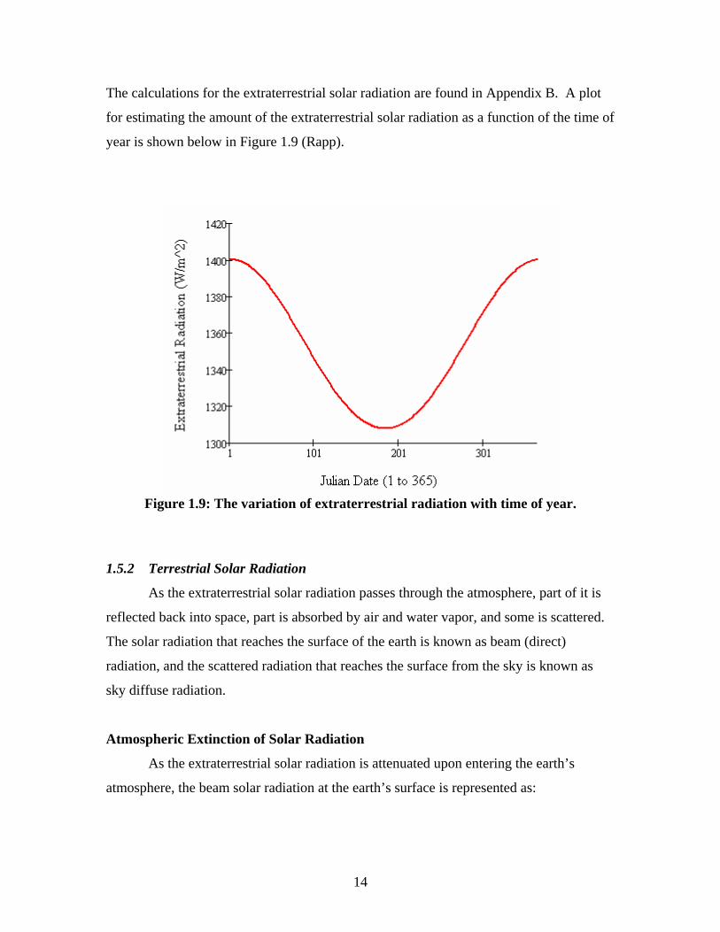
The calculations for the extraterrestrial solar radiation are found in Appendix B. A plot
for estimating the amount of the extraterrestrial solar radiation as a function of the time of
year is shown below in Figure 1.9 (Rapp).
Figure 1.9: The variation of extraterrestrial radiation with time of year.
1.5.2 Terrestrial Solar Radiation
As the extraterrestrial solar radiation passes through the atmosphere, part of it is
reflected back into space, part is absorbed by air and water vapor, and some is scattered.
The solar radiation that reaches the surface of the earth is known as beam (direct)
radiation, and the scattered radiation that reaches the surface from the sky is known as
sky diffuse radiation.
Atmospheric Extinction of Solar Radiation
As the extraterrestrial solar radiation is attenuated upon entering the earth’s
atmosphere, the beam solar radiation at the earth’s surface is represented as:

15
∫=− Kdx
Nb IeI , (1-15)
where Ib,N is the instantaneous beam solar radiation per unit area normal to the suns rays,
K is the local extinction coefficient of the atmosphere, and x is the length of travel
through the atmosphere. Consider the vertical thickness of the atmosphere to be L0 and
the optical depth is represented as:
∫=0
0
L
Kdxk (1-16)
then the beam normal solar radiation for a solar zenith angle is given by:
kmkzk
Nb IeIeIeI −−− === )sin(/)sec(,
α (1-17)
where m, the air mass ratio, is the dimensionless path length of sunlight through the
atmosphere. When the solar altitude angle is 90 degrees (sun directly overhead), the air
mass ratio is equal to one. The values for optical depth (k) were estimated by Threlkeld
and Jordan for average atmospheric conditions at sea level with a moderately dusty
atmosphere and water vapor for the United States. The values for k, along with values for
the sky diffuse factor, C, are given in Table 1.1. In order to amend for differences in
local conditions, the equation for the beam normal solar radiation (Equation 1-17) is
modified by the addition of a parameter called the clearness number, Cn. The resulting
equation is:
)sin(/
,αk
nNb IeCI −= (1-18)
For ease of calculation purposes, the clearness number is assumed to be one.

16
Table 1.1: Average values of atmospheric optical depth (k) and sky diffuse factor (C) for average atmospheric conditions at sea level for the United States (Goswami).
Month Jan Feb Mar Apr May Jun Jul Aug Sep Oct Nov Dec
k 0.142 0.144 0.156 0.180 0.196 0.205 0.207 0.201 0.177 0.160 0.149 0.142
C 0.058 0.060 0.071 0.097 0.121 0.134 0.136 0.122 0.092 0.073 0.063 0.057
Solar Radiation on Clear Days
The total instantaneous solar radiation on a horizontal surface, Ih, is the sum of the
beam radiation, Ib,h, and the sky diffuse radiation, Id,h.
hdhbh III ,, += (1-19)
According to Threlkeld and Jordan, the sky diffuse radiation on a clear day is
proportional to the beam normal solar radiation, and can thus be estimated by use of an
empirical sky diffuse factor, C (see Table 1.1). Thus the total instantaneous solar
radiation can be estimated by
))sin(()cos()cos( )sin(/,,,, αα α +=+=+= − CIeCCIICIzII k
nNbNbNbNbh (1-20)
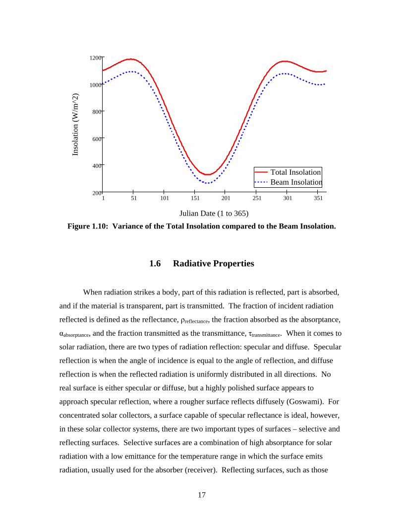
(Goswami) Figure 1.10 shows the variance of the total and beam insolation available
throughout the year.
17
1 51 101 151 201 251 301 351200
400
600
800
1000
1200
Total InsolationBeam InsolationTotal InsolationBeam Insolation
Julian Date (1 to 365)
Inso
latio
n (W
/m^2
)
Figure 1.10: Variance of the Total Insolation compared to the Beam Insolation.
1.6 Radiative Properties
When radiation strikes a body, part of this radiation is reflected, part is absorbed,
and if the material is transparent, part is transmitted. The fraction of incident radiation
reflected is defined as the reflectance, ρreflectance, the fraction absorbed as the absorptance,
αabsorptance, and the fraction transmitted as the transmittance, τtransmittance. When it comes to
solar radiation, there are two types of radiation reflection: specular and diffuse. Specular
reflection is when the angle of incidence is equal to the angle of reflection, and diffuse
reflection is when the reflected radiation is uniformly distributed in all directions. No
real surface is either specular or diffuse, but a highly polished surface appears to
approach specular reflection, where a rougher surface reflects diffusely (Goswami). For
concentrated solar collectors, a surface capable of specular reflectance is ideal, however,
in these solar collector systems, there are two important types of surfaces – selective and
reflecting surfaces. Selective surfaces are a combination of high absorptance for solar
radiation with a low emittance for the temperature range in which the surface emits
radiation, usually used for the absorber (receiver). Reflecting surfaces, such as those

18
required by the solar concentrator, are surfaces with high specular reflectance in the solar
spectrum. Reflecting surfaces are usually highly polished metals or metal coatings on
substrates, some of which are shown in Table 1.2 with the materials reflectivity value.
Under laboratory conditions, polished silver has the highest reflection for the solar energy
spectrum; however, a silvered surface is expensive. Chromium plating, such as that used
in the automotive industry may seem tempting, but it has shown such a low reflectance in
laboratory use that it is usually no longer a consideration for solar reflectance (Goswami).
A better choice, which makes a compromise between price and reflectivity, is the use of a
reflective plastic film known as Aluminized Mylar. Aluminized Mylar is available with a
high reflectance, almost as high as 96% in some cases, and is the choice for design in
many solar collector projects due to the low cost, high reflectivity, and its light-weight
and ease of workability. However, after long exposure to the ultraviolet rays, Aluminized
Mylar tends to degrade, but new stabilizers can be added to aid in slowing the
degradation of the film.
Table 1.2: Specular reflectance values for different reflector materials (Goswami)
Material Reflectivity (ρ)
Copper 0.75
Aluminized type-C Mylar (from Mylar side) 0.76
Gold 0.76±0.03
Various aluminum surfaces-range 0.82-0.92
Anodized aluminum 0.82±0.05
Aluminized acrylic, second surface 0.86
Black-silvered water-white plate glass 0.88Silver (unstable as a front surface mirror) 0.94±0.02
1.7 Solar Collector/Concentrator
The solar collector is the key element in a solar thermal energy system. The
function of the collector is quite simple; it intercepts the incoming solar insolation and
converts it into a useable form of energy that can be applied to meet a specific demand,
19
such as generation of steam from water. Concentrating solar collectors are used to
achieve high temperatures and accomplish this concentration of the solar radiation by
reflecting or refracting the flux incident on the aperture area (reflective surface), Aa onto
a smaller absorber (receiver) area, Ar. The receiver’s surface area is smaller than that of
the reflective surface capturing the energy, thus allowing for the same amount of
radiation that would have been spread over a few square meters to be collected and
concentrated over a much smaller area, allowing for higher temperatures to be obtained.
These concentrating solar collectors have the advantage of higher concentration and are
capable of much greater utilization of the solar intensity at off-noon hours than other
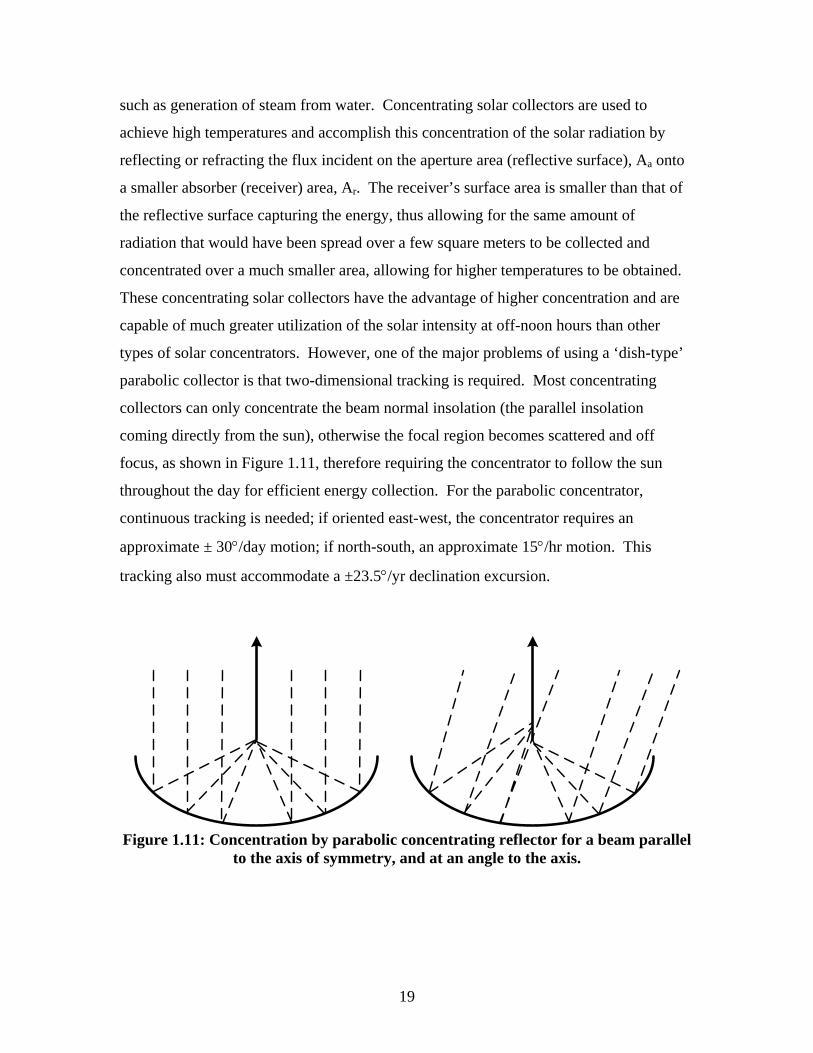
types of solar concentrators. However, one of the major problems of using a ‘dish-type’
parabolic collector is that two-dimensional tracking is required. Most concentrating
collectors can only concentrate the beam normal insolation (the parallel insolation
coming directly from the sun), otherwise the focal region becomes scattered and off
focus, as shown in Figure 1.11, therefore requiring the concentrator to follow the sun
throughout the day for efficient energy collection. For the parabolic concentrator,
continuous tracking is needed; if oriented east-west, the concentrator requires an
approximate ± 30°/day motion; if north-south, an approximate 15°/hr motion. This
tracking also must accommodate a ±23.5°/yr declination excursion.
Figure 1.11: Concentration by parabolic concentrating reflector for a beam parallel
to the axis of symmetry, and at an angle to the axis.

20
As stated previously, the concentration of solar radiation is achieved by reflecting
or refracting the flux incident on an aperture area, Aa, onto a smaller receiver/absorber
area, Ar. There are two ways of representing this ratio of concentration; as an optical
ratio, or as a geometric ratio. An optical concentration ratio, CRo, is defined as the ratio
of the solar flux, Ir, on the receiver to the flux on the aperture, Ia, and is most often
referred to as the flux concentration ratio (Equation 1-21).
a
ro I
ICR = (1-21)
The geometric concentration ratio, CR, is based on the ratio of the area of the aperture
and the receiver.
r
a
AA
CR = (1-22)
The optical concentration ratio gives a true concentration ratio because it takes in account
the optical losses from reflecting and refracting elements. However, it has no
relationship to the receiver area, thus it does not give insight into thermal losses. These
thermal losses are proportional to the receiver area, and since we are most interested in
the thermal aspects of the system, the geometric concentration ratio will be used here.
The amount of solar radiation reaching the receiver is dependent on the amount of
radiation available (sky conditions), the size of the concentrator, and several other
parameters describing the loss of this radiation on its way to being absorbed. Heat loss
from the receiver is separated into convection-conduction heat loss and radiation heat
loss. The rate of heat loss increases as the area of the receiver and/or its temperature
increases. This is why concentrators are more efficient at a given temperature than flat
plate collectors, because the area in which heat is lost is smaller than the aperture area.
The useful energy delivered by the collector, qu, is given by the energy balance
raccacou ATTUAIq )( −−=η (1-23)

21
where ηo is the optical efficiency, Uc is the collector heat-loss conductance, Tc and Ta
respectively are the temperatures of the collector and the ambient temperature, and Ic is
the insolation incident on the aperture. The instantaneous collector efficiency, ηc, is thus
given by
CRITTU
c
accoc
1)( −−=ηη (1-24)
Neglecting the optical efficiency, the instantaneous efficiency, ηinst, of the solar thermal
collector can also be simplified and defined as the ratio of the useful heat,Q& , delivered
per aperture area, Aa, and the insolation, Ic, which is incident on the aperture.
ccinst I
qAIQ &&
==η (1-25)
The useful heat Q& is related to the flow rate, m& , specific heat at a constant pressure, Cp,
and the inlet and outlet temperatures, Tin and Tout, by
TCmTTCmQ pinoutp Δ=−= &&& )( (1-26)
(Hsieh, Duffie)
1.7.1 Acceptance Angle
Closely related to the concentration ratio is the acceptance angle, 2θa. The acceptance
angle is defined as being the angular range over which all or most all of the rays are
accepted without moving the collector (Rabl). The higher the concentration, the smaller
the range of acceptance angles by the collector, thus an inverse relationship between the
concentration and the acceptance aperture of the collector exists. As was stated in a
previous section, tracking is needed for the system to maintain the high solar
concentration, thus it is desirable to have a collector that has as high an acceptance angle
as possible. The basic expression given by Rabl for acceptance angle is:

22
The maximum possible concentration achievable with a collector that only
accepts all incident light rays within the half-angle,θa, is
)(sin1
2a
idealCRθ
= (1-27)
for a three dimensional collector (parabolic ‘dish-type’ concentrator) (Rabl).
The derivation of this equation can be found in Appendix A.
1.7.2 Thermodynamic Limits of Concentration (Max Achievable Temperature)
As stated previously, there is a thermodynamic limit to the concentration of a
concentrating solar collector, or more plainly stated, a maximum achievable temperature.
From the laws of thermodynamics, sabs TT ≤ , where Tabs is the temperature of the absorber
(receiver) and Ts is the temperature of the sun. If Tabs were greater than Ts, then the
system would be in violation of the second law (Rapp). The power absorbed by the
receiver can be defined by the following equation:
σθηση 4242
2
)(sin sopitcalsopticalabss TATRrAQ ==→ (1-28)
When using the source as the sun, the appropriate half-angle is o
41≈θ (Rapp). The
radiative power loss from the absorber is
4
absabsabsambabs TAQ σε=→ (1-29)
where εabs is the effective emissivity of the receiver over the spectral wavelength region
characteristic of a body emitting at Tabs. If the efficiency of the collector for capturing the
incident radiation as useful energy in a transfer fluid is called η, then the heat balance on
the absorber is:
ambsambabsabss QQQ →→→ += η (1-30)

23
To simplify the calculations, it will be assumed that there are no conductive or convective
heat losses from the receiver, thus
442 )(sin)1( absabsabssoptical TATA σεθσηη =− (1-31)
This can also be written as
41
)(sin)1( 2⎥⎦
⎤⎢⎣
⎡−= θ
εη
η ltheoreticaabs
opticalsabs CRTT (1-32)
where CRideal was defined in Equation 1-27, and CRtheoretical is equal to the geometric
concentration ratio, therefore,
41
)1( ⎥⎦
⎤⎢⎣
⎡−=
ideal
ltheoretica
abs
opticalsabs CR
CRTT
εη
η (1-33)
The maximum possible value of CRtheoretical is CRideal, and the maximum value of Tabs is
Ts. This, however, can only occur if the optics of the concentrator are perfect and no
useful heat is lost or removed from the receiver. If this were the case, and considering
the sun to be represented as a blackbody at 5760 K, the maximum achievable temperature
at the receiver would be equivalent to that of the sun (Rapp).
1.8 The Receiver/Absorber
The purpose of the receiver in the solar-thermal system is to intercept and absorb
the concentrated solar radiation and convert it to usable energy; in this case, thermal
energy which will then be converted to electrical energy via a thermodynamic cycle.
Once absorbed, this thermal energy is transferred as heat to a heat-transfer fluid, such as
water, Paratherm ©, ethyl-glycol, or molten salt, to be stored and/or used in a power
conversion cycle.
24
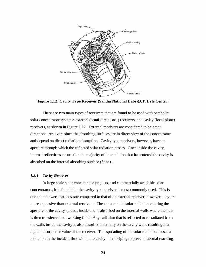
Figure 1.12: Cavity Type Receiver (Sandia National Labs)(J.T. Lyle Center)
There are two main types of receivers that are found to be used with parabolic
solar concentrator systems: external (omni-directional) receivers, and cavity (focal plane)
receivers, as shown in Figure 1.12. External receivers are considered to be omni-
directional receivers since the absorbing surfaces are in direct view of the concentrator
and depend on direct radiation absorption. Cavity type receivers, however, have an
aperture through which the reflected solar radiation passes. Once inside the cavity,
internal reflections ensure that the majority of the radiation that has entered the cavity is
absorbed on the internal absorbing surface (Stine).
1.8.1 Cavity Receiver
In large scale solar concentrator projects, and commercially available solar
concentrators, it is found that the cavity type receiver is most commonly used. This is
due to the lower heat-loss rate compared to that of an external receiver; however, they are
more expensive than external receivers. The concentrated solar radiation entering the
aperture of the cavity spreads inside and is absorbed on the internal walls where the heat
is then transferred to a working fluid. Any radiation that is reflected or re-radiated from
the walls inside the cavity is also absorbed internally on the cavity walls resulting in a
higher absorptance value of the receiver. This spreading of the solar radiation causes a
reduction in the incident flux within the cavity, thus helping to prevent thermal cracking

25
or smelting of the internal walls. Also, because of the design of the cavity receiver, it is
easier to insulate to aid in avoiding radiant and convective heat loss to the environment.
(Kribus)
1.8.2 External Receiver
External receivers are designed to absorb radiation coming from all directions and
are the simpler of the two receiver types. The size of the receiver is determined in a
process based on the amount of received solar radiation and the amount of heat loss from
the receiver. Simply stated, a larger receiver will capture more reflected solar radiation,
but will suffer from more radiant and convective heat loss. These receivers are nominally
spherical or tubular in shape. (J.T. Lyle Center)
1.9 Heat Storage
There are three methods for storing the collected thermal energy: 1) sensible, 2)
latent, and 3) thermochemical heat storage. These methods differ in the amount of heat
that can be stored per unit weight or volume of storage media and operating temperatures.
Thermochemical is not practical for the solar thermal system discussed in this paper, thus
a discussion will be omitted. (Rapp)
1.9.1 Sensible Heat Storage
In sensible heat storage, the thermal energy is stored by changing the temperature
of the storage medium. The amount of heat stored depends on the heat capacity of the
media being used, the temperature change, and the amount of storage media. Solid or
liquid state media can be utilized, however, since storage occurs over a temperature
interval, temperature regulation during retrieval can prove to be problematic. The most
common type of sensible heat storage is that of a liquid in a drum in which heat is
constantly added and is often recirculated. (Rapp)
26
1.9.2 Latent Heat Storage
In latent heat storage, thermal energy is stored by a means of a reversible change
of state (phase change) in the media. Solid-liquid transformations are most commonly
utilized. Liquid-gas and solid-gas phase changes involve the most energy of the possible
latent heat storage methods. A common media used for latent heat storage in solar
thermal systems is molten salt. A good example of this is that a pint bottle of molten salt
at 30°C releases 0.1515 MJ on cooling to room temperature (and will feel tepid to the
touch), whereas the same bottle filled with water at 60°C only releases half the amount of
heat on cooling (and is hot to the touch). This is one main advantage to latent heat
storage when compared to other methods, that is has a higher heat capacity, thus allowing
for a smaller thermal storage unit. (Goswami, Lane)
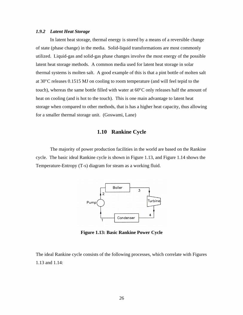
1.10 Rankine Cycle
The majority of power production facilities in the world are based on the Rankine
cycle. The basic ideal Rankine cycle is shown in Figure 1.13, and Figure 1.14 shows the
Temperature-Entropy (T-s) diagram for steam as a working fluid.
Figure 1.13: Basic Rankine Power Cycle
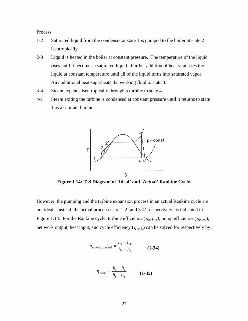
The ideal Rankine cycle consists of the following processes, which correlate with Figures
1.13 and 1.14:
27
Process
1-2 Saturated liquid from the condenser at state 1 is pumped to the boiler at state 2
isentropically
2-3 Liquid is heated in the boiler at constant pressure. The temperature of the liquid
rises until it becomes a saturated liquid. Further addition of heat vaporizes the
liquid at constant temperature until all of the liquid turns into saturated vapor.
Any additional heat superheats the working fluid to state 3.
3-4 Steam expands isentropically through a turbine to state 4.
4-1 Steam exiting the turbine is condensed at constant pressure until it returns to state
1 as a saturated liquid.
Figure 1.14: T-S Diagram of ‘Ideal’ and ‘Actual’ Rankine Cycle.
However, the pumping and the turbine expansion process in an actual Rankine cycle are
not ideal. Instead, the actual processes are 1-2’ and 3-4’, respectively, as indicated in
Figure 1.14. For the Rankine cycle, turbine efficiency (ηturbine), pump efficiency (ηpump),
net work output, heat input, and cycle efficiency (ηcycle) can be solved for respectively by:
43
'43_ hh
hhthermalturbine −
−=η (1-34)
'21
21
hhhh
pump −−
=η (1-35)
28
)()(OutputNet Work 1'2'43 hhhh −−−= (1-36)
'23InputHeat hh −= (1-37)
pump
PPhhη
υ )( WorkPump 121'2
−=−= (1-38)
'23
1'2'43cycle
)()(InputHeat
OutputNet Work Efficiency Cyclehh
hhhh−
−−−===η (1-39)
where h is the enthalpy and υ is the specific volume at state 1 (Van Wylen).
For comparison purposes, the Rankine cycle efficiency of standard power plants
is compared with that of the systems Carnot cycle efficiency, where the Carnot efficiency
is given as:
H
CCarnot T
T−== 1EfficiencyCarnot η (1-40)
where TC is the condenser temperature (low rejection temperature) of the system, and TH
is the input temperature of the system (Cengel). The majority of standard steam power
plants attempt to operate at an efficiency of 50 percent of its Carnot efficiency
(Powerfromthesun). The lower efficiency of the Rankine cycle compared to that of the
Carnot cycle is due to the average temperature between points 2 and 2’ being less than
the temperature during the evaporation stage. Even with the lower efficiency, the
Rankine cycle is still used over the Carnot cycle for a few reasons. The first is due to the
pumping process, where at state 1 there is a mixture of liquid and vapor. It is difficult to
design a pump which can handle the mixture of water and vapor at this stage and deliver
the working fluid as a saturated liquid at stage 2’. It is easier to condense the vapor
completely and have the pump only handle liquid. Secondly, in the Carnot cycle, the heat
transfer is at a constant temperature, therefore the vapor is superheated in process 3-3”,
where as in the Rankine cycle, the fluid is superheated at constant pressure in process 3-

29
3’. Thus, in the Carnot cycle, the pressure is dropping, which means that the heat must
be transferred to the fluid (vapor at this stage) as it undergoes an expansion process in
which work is done. It is very difficult to achieve this heat transfer in practice, hence
why the Rankine cycle is used (Van Wylen).
1.10.1 Working Fluid
In a solar Rankine cycle, the working fluid is chosen based upon the expected
temperatures of the solar collection system. Steam (water) is most commonly used with
the Rankine cycle due to its critical temperature and pressure of 374°C and 22.1 MPa
respectively. Thus it is usable in systems that operate at high temperatures, such as those
produced by parabolic ‘dish’ type collector systems. When water is converted to steam,
its volume is increased by approximately 1600 times (Sebastian). This expansion is what
stores the energy and produces the force to run a steam turbine. Other major advantages
of steam is that it is non-toxic, environmentally safe, inexpensive, and nominally easily
available. However, due to its low molecular weight, extremely high turbine speeds are
required to achieve high turbine efficiencies (Goswami).
1.10.2 Deviation of Actual Cycle from Ideal
Piping Losses
In the actual Rankine cycle, there are losses which are contributed by the piping,
such as pressure drops caused by frictional effects and heat transfer to the surroundings.
Consider the pipe connecting the turbine to the boiler, in only frictional effects occur,
states a and b, in Figure 1.15, represent the states of the steam leaving the boiler and
entering the turbine. These friction effects in turn cause an increase in the entropy. Heat
transferred to the surroundings at constant pressure is represented by process b-c, also
shown in Figure 1.15. This effect in turn causes a decrease in entropy. Both the pressure
drop and heat transfer causes a decrease in availability of steam entering the turbine.
(Van Wylen)

30
250
300
350
400
450
500
550
600
650
700
-1 0 1 2 3 4 5 6 7 8 9 10 Figure 1.15: Temperature-entropy diagram showing effect of losses between boiler
and turbine.
Pump and Turbine Losses
Losses in the turbine are nominally associated with the flow of the working fluid
through the turbine. Heat transfer to the surroundings also plays a role, but is usually of
secondary importance. These effects are basically the same as for those mentioned in the
section above about piping losses. This process is shown in Figure 1.14, where point 4s
represent the state after an isentropic expansion and point 4’ represents the actual state
leaving the turbine. Losses in the turbine are also caused by any kind of throttling control
or resistance on the output shaft. Losses in the pump are similar to those mentioned here
of the turbine and are due to the irreversibility associated with the fluid flow. (Van
Wylen, Cengal)
1.11 Steam Turbine
With the process steam that is generated by the solar thermal system, the potential
energy of this steam must somehow be extracted. This energy can by extracted by
expanding the steam through a turbine. An ideal steam turbine is considered to be an
isentropic process (or constant entropy process) in which the entropy of the steam
entering the turbine is equal to that of the entropy of the steam exiting the turbine.
T
s
ab
c

31
However, no steam turbine is truly isentropic, but depending on application, efficiencies
ranging from 20 to 90 percent can be achieved (Salisbury). There are two general
classifications of steam turbines, impulse and reaction turbines, as shown in Figure 1.16.
Figure 1.16: Diagram showing difference between
an impulse and a reaction turbine.
1.11.1 Impulse Turbine
An impulse turbine is driven by one or more high-speed free jets. The jets are
accelerated in nozzles, which are external to the turbine rotor (wheel) and impinge the
flow on the turbine blades, sometimes referred to as ‘buckets’. As described by
Newton’s second law of motion, this impulse removes the kinetic energy from the steam
flow by the resulting force on the turbine blades causing the rotor to spin, resulting in
shaft rotation.
1.11.2 Reaction Turbine
In a reaction turbine, the rotor blades are designed so as to be convergent nozzles,
thus the pressure change takes place both externally and internally. External acceleration
takes place, the same as in an impulse turbine, with additional acceleration from the
moving blades of the rotor. (Fox and McDonald)

32
1.11.3 Turbine Efficiency
In order to determine the efficiency of a turbine, certain assumptions have to be
made. It needs to be assumed that the process through the turbine is a steady-state,
steady-flow process, meaning that 1) the control volume does not move relative to the
coordinate frame, 2) the state of the mass at each point in the control volume does not
vary with time, and 3) the rates at which heat and work cross the control surface remain
constant (Van Wylen et al). The repercussions of these assumptions are that 1) all
velocities measured relative to the coordinate frame are also velocities relative to the
control surface, and there is no work associated with the acceleration of the control
volume, 2) the state of mass at each point in the control volume does not vary with time
such that
0=dtdm (1-41) and 0=
dtdE (1-42)
resulting in the continuity equation
∑ ∑= outletinlet mm && (1-43)
and the first law as
WgZV
hmgZV
hmQ outletoutlet
outletinletinlet
inlet&&&& +⎟⎟
⎠
⎞⎜⎜⎝
⎛++=⎟⎟
⎠
⎞⎜⎜⎝
⎛+++ ∑∑ 22
22
(1-44)
and 3) the applications of equations 1-43 and 1-44 above are independent of time.
Equation 1-44 can then be rearranged, yielding
wgZV
hgZV
hq outletoutlet
outletinletinlet
inlet +++=+++22
22
(1-45)
where

33
mQq&
&= (1-46) and
mWw&
&= (1-47),
the heat transfer and work per unit mass flowing into and out of the turbine. The
efficiency of the turbine is then determined as being the actual work done per unit mass
of steam flow through the turbine, wa, compared to that work that would be done in an
ideal cycle, ws. The efficiency of the turbine (Van Wylen) is then expressed as:
s
aturbine w
w=η (1-48)
1.12 Overview
The overall objective of this project is to design a system that is capable of power
generation by means of solar concentration for use in emergency and/or off-grid
situations, which would be reasonably affordable for newly developing regions of the
world. The system must be capable of utilizing nearby resources, such as well water, or
unfiltered stream water, and must be ‘simple’ in design for simplicity of repairs.
However, in order to reach this goal, a few key research objectives must be met. The key
objectives include characterization of the dish, the receiver, and the turbine in order to
determine the overall system efficiency. This characterization of the individual
components of the system will allow for future work on the project for an increase in
efficiency and power output.
34
CHAPTER 2
EXPERIMENTAL APPARATUS AND PROCEDURES
2.1 Introduction
This work was focused on the development of a system for converting incoming
solar radiation to electrical energy. The system concentrated the incoming solar radiation
to power a thermal cycle in which the energy was converted to mechanical power, and
subsequently to electrical power. This chapter contains a description of this system and a
detailed explanation of how the individual components of the system work. The design,
implementation, and testing of the system were conducted at the Sustainable Energy
Science and Engineering Center (SESEC) located on the campus of Florida State
University in Tallahassee, Florida.
2.2 Solar Collector
To obtain the high temperatures necessary, a concentrating solar collector is
needed due to solar radiation being a low entropy heat source. The type chosen was that
of the parabolic ‘dish’ type. The parabolic dish is a 3.66 meter diameter Channel Master
Satellite dish, obtained from WCTV Channel 6 of Tallahassee, Florida. The dish consists
of six fiberglass, pie-shaped, sections which are assembled together to form the parabolic
structure of the dish. Figure 2.1a shows one of the pie shaped panels of the dish. With
the six panels assembled, shown in Figure 2.1b, the dish has a surface area of 11.7 m2
(126.3 ft2), with an aperture area of 10.51 m2 (113.1 ft2) and a focal length of 1.34 meters
(52.75 inches).

35
Figure 2.1: a) Pie-shaped section of the dish coated in Aluminized Mylar.
b) Assembled dish with surface area of 11.7 m2.
Because the dish was originally surfaced to reflect radio waves, a new surface
capable of reflecting the ultraviolet to the infrared spectrum (electromagnetic radiation
between the wavelengths of 300 to 200 nm) was needed; basically, a surface with high
visual reflectivity. Because of its low cost, ease of workability, and high reflectivity of
0.76, Aluminized Mylar was chosen as the new surface coating of the dish. For
application of the Aluminized Mylar to the fiberglass panels, the mylar was cut into 152.4
x 152.4 mm (6 x 6 in) squares, and a heavy duty double sided adhesive film by Avery
Denison products was used, as shown in Figure 2.2.
Figure 2.2: Application of Aluminized Mylar to Fiberglass Panels of the Dish
36
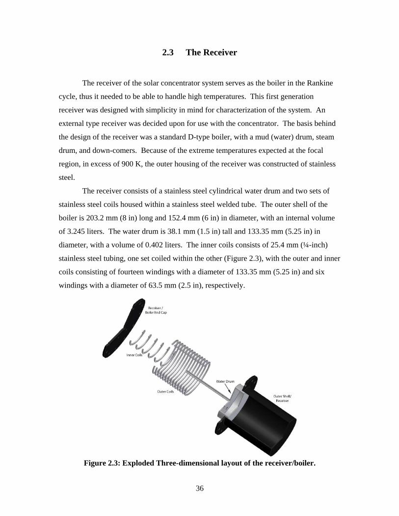
2.3 The Receiver
The receiver of the solar concentrator system serves as the boiler in the Rankine
cycle, thus it needed to be able to handle high temperatures. This first generation
receiver was designed with simplicity in mind for characterization of the system. An
external type receiver was decided upon for use with the concentrator. The basis behind
the design of the receiver was a standard D-type boiler, with a mud (water) drum, steam
drum, and down-comers. Because of the extreme temperatures expected at the focal
region, in excess of 900 K, the outer housing of the receiver was constructed of stainless
steel.
The receiver consists of a stainless steel cylindrical water drum and two sets of
stainless steel coils housed within a stainless steel welded tube. The outer shell of the
boiler is 203.2 mm (8 in) long and 152.4 mm (6 in) in diameter, with an internal volume
of 3.245 liters. The water drum is 38.1 mm (1.5 in) tall and 133.35 mm (5.25 in) in
diameter, with a volume of 0.402 liters. The inner coils consists of 25.4 mm (¼-inch)
stainless steel tubing, one set coiled within the other (Figure 2.3), with the outer and inner
coils consisting of fourteen windings with a diameter of 133.35 mm (5.25 in) and six
windings with a diameter of 63.5 mm (2.5 in), respectively.
Figure 2.3: Exploded Three-dimensional layout of the receiver/boiler.

37
The outer shell is filled with a molten salt into which the water drum and coils are
submerged. The molten salt is known as Draw Salt, which consists of a 1:1 molar ratio
of Potassium Nitrate (KNO3 - 101.11 grams per mol) and Sodium Nitrate (NaNO3 - 84.99
grams per mol). There is a total of 19.39 Mols of Draw Salt in the thermal bath, Figure
2.4, which has a total mass of 3.61 kg; 1.96 kg of Potassium Nitrate and 1.65 kg of
Sodium Nitrate. The Draw Salt serves as latent heat storage to allow for continuous heat
transfer in the case of intermittent cloud cover and for equal thermal distribution over the
water drum and the coils.
Figure 2.4: The Draw Salt mixture being mixed in the receiver.
The receiver is set up to record the inlet, outlet, and thermal bath temperatures,
along with the outlet steam pressure. Three stainless steel sleeved K-type thermocouples,
with ceramic connectors, are used for temperature measurements. The thermocouples are
located at the inlet and exit of the receiver to measure the incoming water and exiting
steam temperature. The third thermocouple is submerged halfway into the thermal Draw
Salt bath. Figure 2.5 shows the location of the thermocouples on the receiver. With the
receiver assembled, it was then placed at the focal region of the concentrator. The
supporting structure for the receiver and the area of the receiver not subject to
concentrated solar intensity was then covered with Kaowool Superwool insulation;
shown in Figure 2.6.

38
Figure 2.5: Schematic of Instrumentation of Boiler. TC1 is inlet temperature, TC2
is exit temperature, and TC3 is the temperature of the thermal Draw Salt bath. The pressure transducer measures the exit pressure of the boiler.
Figure 2.6: Receiver assembled and positioned in focal region of concentrator.
Receiver and supporting structure of receiver wrapped in super wool insulation.
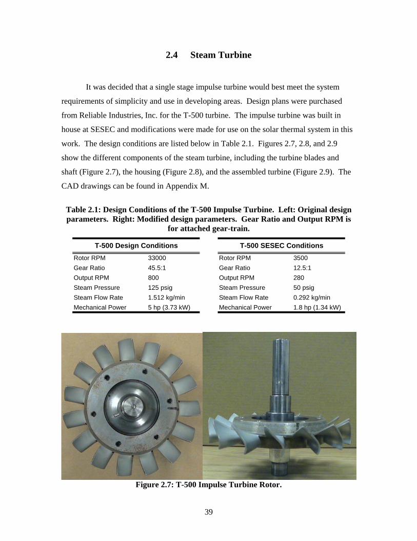
39
2.4 Steam Turbine
It was decided that a single stage impulse turbine would best meet the system
requirements of simplicity and use in developing areas. Design plans were purchased
from Reliable Industries, Inc. for the T-500 turbine. The impulse turbine was built in
house at SESEC and modifications were made for use on the solar thermal system in this
work. The design conditions are listed below in Table 2.1. Figures 2.7, 2.8, and 2.9
show the different components of the steam turbine, including the turbine blades and
shaft (Figure 2.7), the housing (Figure 2.8), and the assembled turbine (Figure 2.9). The
CAD drawings can be found in Appendix M.
Table 2.1: Design Conditions of the T-500 Impulse Turbine. Left: Original design parameters. Right: Modified design parameters. Gear Ratio and Output RPM is
for attached gear-train.
Rotor RPM 33000Gear Ratio 45.5:1Output RPM 800Steam Pressure 125 psigSteam Flow Rate 1.512 kg/minMechanical Power 5 hp (3.73 kW)
T-500 Design Conditions
Rotor RPM 3500Gear Ratio 12.5:1Output RPM 280Steam Pressure 50 psigSteam Flow Rate 0.292 kg/minMechanical Power 1.8 hp (1.34 kW)
T-500 SESEC Conditions
Figure 2.7: T-500 Impulse Turbine Rotor.
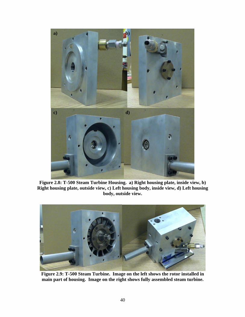
40
Figure 2.8: T-500 Steam Turbine Housing. a) Right housing plate, inside view, b)
Right housing plate, outside view, c) Left housing body, inside view, d) Left housing body, outside view.
Figure 2.9: T-500 Steam Turbine. Image on the left shows the rotor installed in main part of housing. Image on the right shows fully assembled steam turbine.
a) b)
c) d)

41
2.5 Gear-Train
Although the steam turbine is capable of achieving high speeds, it is a very low
torque device. Very high speed and low torque is a bad combination for use in a power
generating system, although the higher speeds are needed to produce higher voltages;
when a load is added to the generator, more torque is needed to overcome the load and
produce the required current. Thus, for power production, it is ideal to have a shaft
output that is more balanced, with a moderate rotational speed and torque. It is possible
to achieve this by combining the steam turbine with a gear train.
Through the use of a gear train, the high speed and low torque of the steam
turbine can be converted to low or moderate speeds with high to moderate torque. The
gear train used here is a compound gear train consisting of two stages, with a total gear
ratio of 12.5. The first stage (high speed stage) of the gear train consists of a high speed
pinion spur gear with 22 teeth. The reduction gear in this first stage consists of 80 teeth,
resulting in a 3.64 gear ratio. The second stage (intermediate speed stage) consists of an
intermediate pinion gear of 21 teeth, and an intermediate gear with 72 teeth, for the
resultant gear ratio of 12.5. This reduction slows the turbine shaft speed from a range of
3000 to 4000 rpm, to a more feasible range of 150 to 350 rpm. Figure 2.10 shows the
assembly of the different stages of drive train and Figure 2.11 shows the fully assembled
steam turbine and gear train. The CAD for the gear train can be found along with the
CAD of the steam turbine in Appendix M.
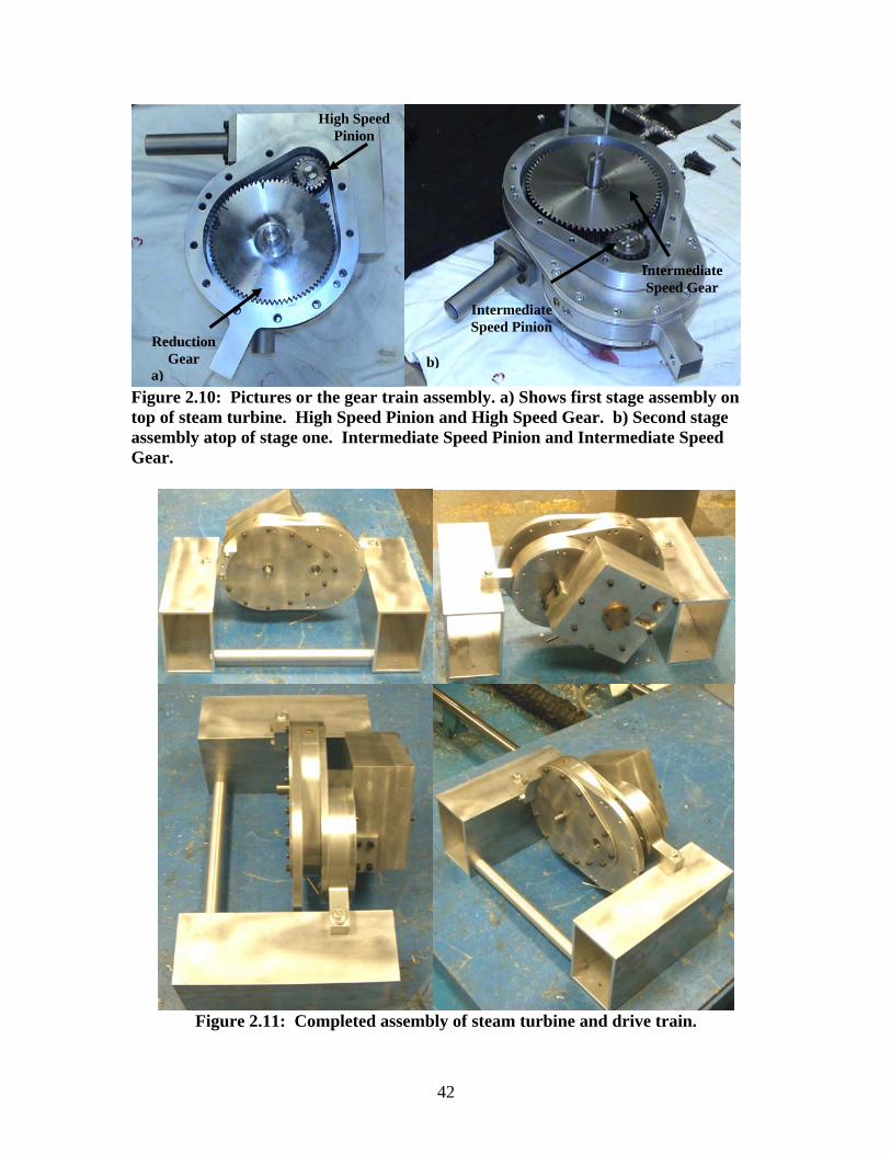
42
Figure 2.10: Pictures or the gear train assembly. a) Shows first stage assembly on top of steam turbine. High Speed Pinion and High Speed Gear. b) Second stage assembly atop of stage one. Intermediate Speed Pinion and Intermediate Speed Gear.
Figure 2.11: Completed assembly of steam turbine and drive train.
High Speed Pinion
Reduction Gear
Intermediate Speed Pinion
Intermediate Speed Gear
a) b)

43
2.6 Working Fluid of Solar Thermal System
Since the design of this system was to be kept as simple as possible, water was
chosen as the working fluid. If the system were set up off-grid in a field, then a well
could be used to supply water for the solar thermal system. In the event that a water-well
is unavailable, as was the case here, a reservoir for the water is needed. A steel
constructed tank (Figure 2.12), with a capacity of 13 liters (~ 3.43 gallons) is used.
Because of the conditions for which the system was designed, such as off-grid and
emergency use, the water does not need filtered. However, if the water being used is full
of debris, maintenance of the system will need to be performed more frequently, thus the
use of a screen over the inlet supply line of the pump is suggested, but not necessary.
Figure 2.12: Water Tank used for supply water; wrapped in super wool insulation. a) Water line to pump, b) Return inlet from steam turbine, c) Thermocouple insert.
a)
c) b)
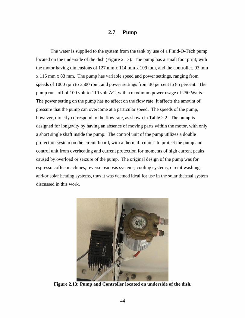
44
2.7 Pump
The water is supplied to the system from the tank by use of a Fluid-O-Tech pump
located on the underside of the dish (Figure 2.13). The pump has a small foot print, with
the motor having dimensions of 127 mm x 114 mm x 109 mm, and the controller, 93 mm
x 115 mm x 83 mm. The pump has variable speed and power settings, ranging from
speeds of 1000 rpm to 3500 rpm, and power settings from 30 percent to 85 percent. The
pump runs off of 100 volt to 110 volt AC, with a maximum power usage of 250 Watts.
The power setting on the pump has no affect on the flow rate; it affects the amount of
pressure that the pump can overcome at a particular speed. The speeds of the pump,
however, directly correspond to the flow rate, as shown in Table 2.2. The pump is
designed for longevity by having an absence of moving parts within the motor, with only
a short single shaft inside the pump. The control unit of the pump utilizes a double
protection system on the circuit board, with a thermal ‘cutout’ to protect the pump and
control unit from overheating and current protection for moments of high current peaks
caused by overload or seizure of the pump. The original design of the pump was for
espresso coffee machines, reverse osmosis systems, cooling systems, circuit washing,
and/or solar heating systems, thus it was deemed ideal for use in the solar thermal system
discussed in this work.
Figure 2.13: Pump and Controller located on underside of the dish.
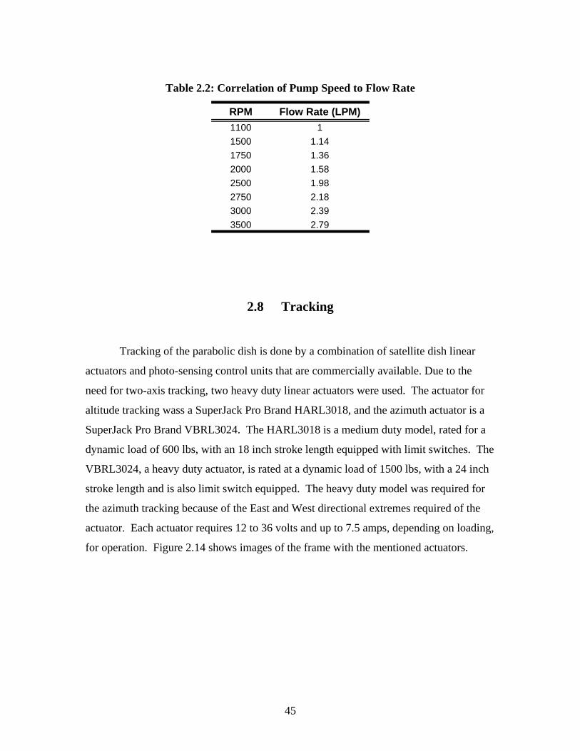
45
Table 2.2: Correlation of Pump Speed to Flow Rate
RPM Flow Rate (LPM)1100 11500 1.141750 1.362000 1.582500 1.982750 2.183000 2.393500 2.79
2.8 Tracking
Tracking of the parabolic dish is done by a combination of satellite dish linear
actuators and photo-sensing control units that are commercially available. Due to the
need for two-axis tracking, two heavy duty linear actuators were used. The actuator for
altitude tracking wass a SuperJack Pro Brand HARL3018, and the azimuth actuator is a
SuperJack Pro Brand VBRL3024. The HARL3018 is a medium duty model, rated for a
dynamic load of 600 lbs, with an 18 inch stroke length equipped with limit switches. The
VBRL3024, a heavy duty actuator, is rated at a dynamic load of 1500 lbs, with a 24 inch
stroke length and is also limit switch equipped. The heavy duty model was required for
the azimuth tracking because of the East and West directional extremes required of the
actuator. Each actuator requires 12 to 36 volts and up to 7.5 amps, depending on loading,
for operation. Figure 2.14 shows images of the frame with the mentioned actuators.
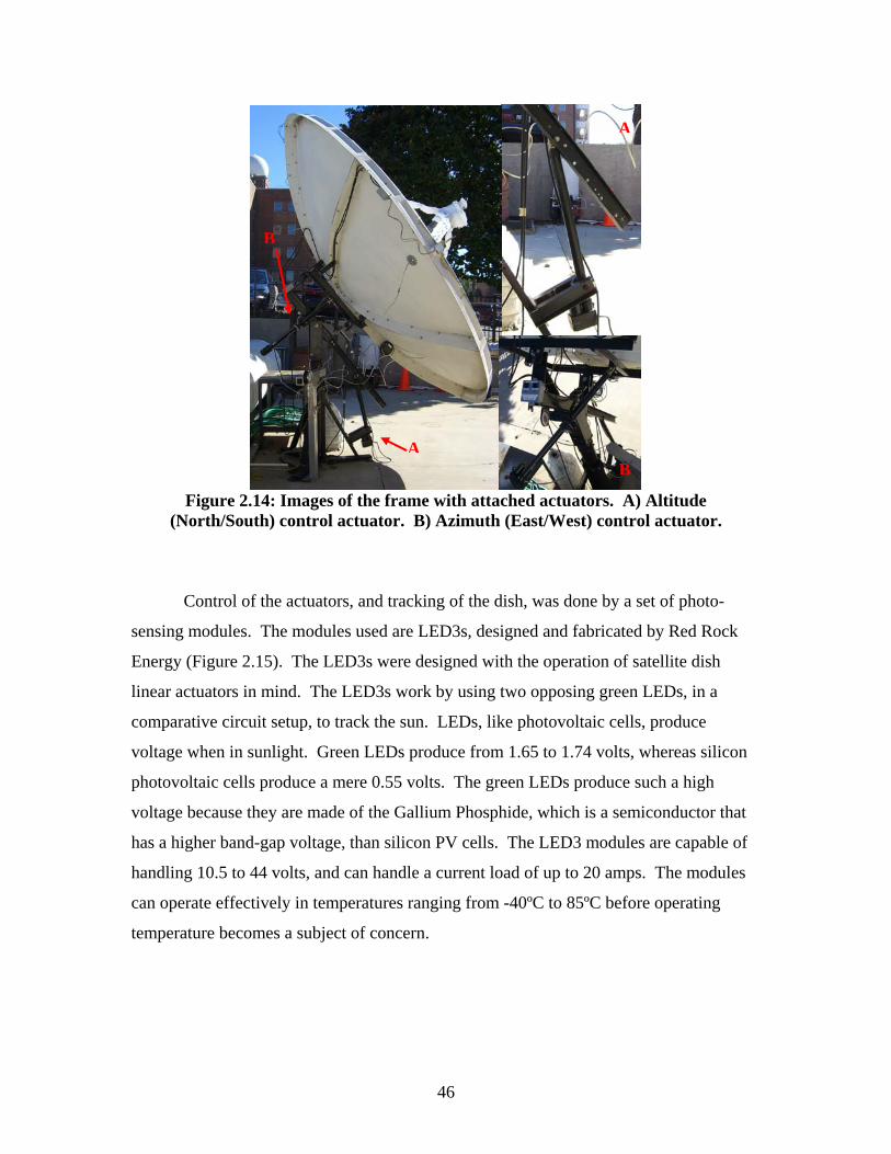
46
Figure 2.14: Images of the frame with attached actuators. A) Altitude
(North/South) control actuator. B) Azimuth (East/West) control actuator.
Control of the actuators, and tracking of the dish, was done by a set of photo-
sensing modules. The modules used are LED3s, designed and fabricated by Red Rock
Energy (Figure 2.15). The LED3s were designed with the operation of satellite dish
linear actuators in mind. The LED3s work by using two opposing green LEDs, in a
comparative circuit setup, to track the sun. LEDs, like photovoltaic cells, produce
voltage when in sunlight. Green LEDs produce from 1.65 to 1.74 volts, whereas silicon
photovoltaic cells produce a mere 0.55 volts. The green LEDs produce such a high
voltage because they are made of the Gallium Phosphide, which is a semiconductor that
has a higher band-gap voltage, than silicon PV cells. The LED3 modules are capable of
handling 10.5 to 44 volts, and can handle a current load of up to 20 amps. The modules
can operate effectively in temperatures ranging from -40ºC to 85ºC before operating
temperature becomes a subject of concern.
A
B
B
A
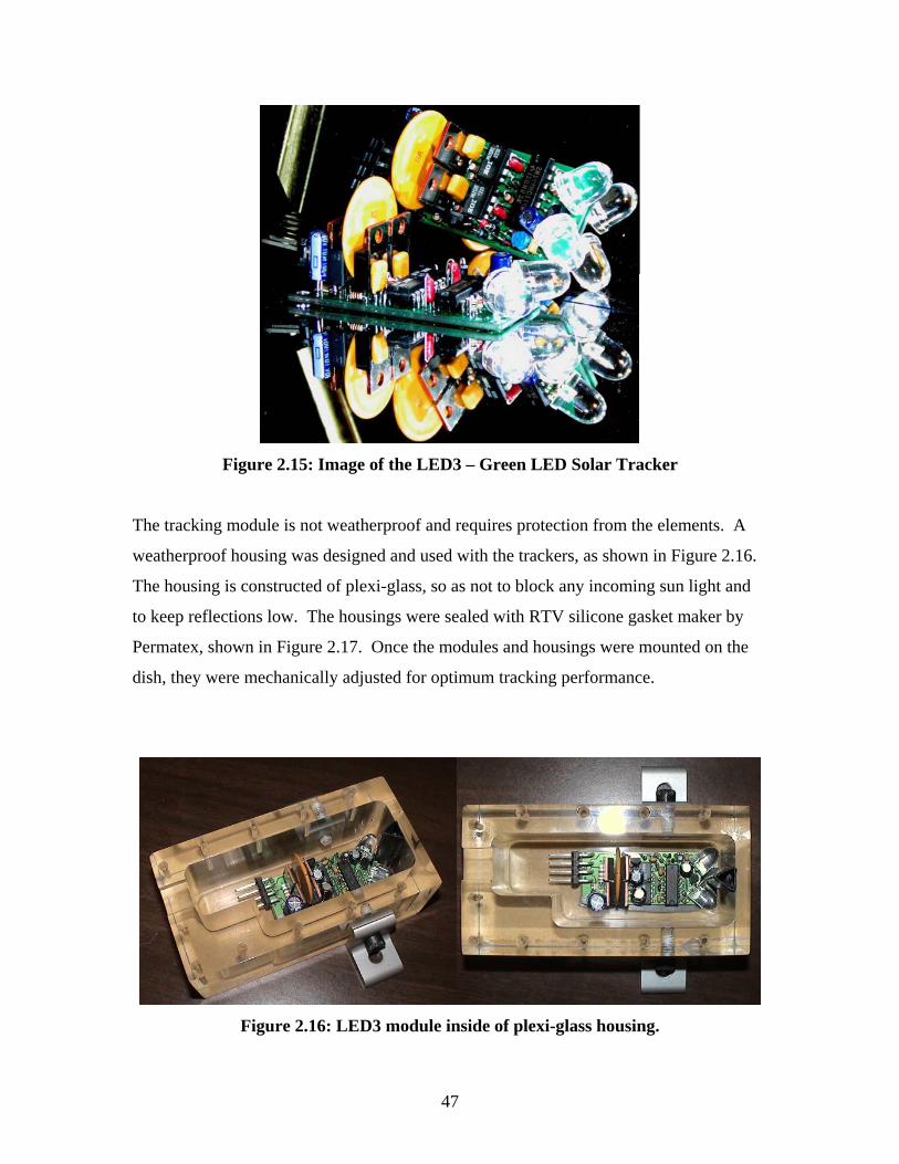
47
Figure 2.15: Image of the LED3 – Green LED Solar Tracker
The tracking module is not weatherproof and requires protection from the elements. A
weatherproof housing was designed and used with the trackers, as shown in Figure 2.16.
The housing is constructed of plexi-glass, so as not to block any incoming sun light and
to keep reflections low. The housings were sealed with RTV silicone gasket maker by
Permatex, shown in Figure 2.17. Once the modules and housings were mounted on the
dish, they were mechanically adjusted for optimum tracking performance.
Figure 2.16: LED3 module inside of plexi-glass housing.

48
Figure 2.17: LED3 module sealed in plexi-glass housing.
To improve the accuracy, shading was later added to the trackers on the dish. The tracker
module housings were also painted white to help reflect heat from the modules. This is
shown in Figure 2.18 below.
Figure 2.18: Tracker module housing painted white and shading added.
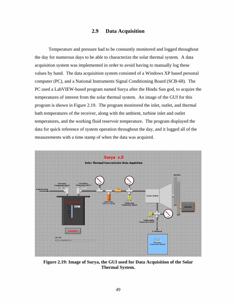
49
2.9 Data Acquisition
Temperature and pressure had to be constantly monitored and logged throughout
the day for numerous days to be able to characterize the solar thermal system. A data
acquisition system was implemented in order to avoid having to manually log these
values by hand. The data acquisition system consisted of a Windows XP based personal
computer (PC), and a National Instruments Signal Conditioning Board (SCB-68). The
PC used a LabVIEW-based program named Surya after the Hindu Sun god, to acquire the
temperatures of interest from the solar thermal system. An image of the GUI for this
program is shown in Figure 2.19. The program monitored the inlet, outlet, and thermal
bath temperatures of the receiver, along with the ambient, turbine inlet and outlet
temperatures, and the working fluid reservoir temperature. The program displayed the
data for quick reference of system operation throughout the day, and it logged all of the
measurements with a time stamp of when the data was acquired.
Figure 2.19: Image of Surya, the GUI used for Data Acquisition of the Solar
Thermal System.

50
2.9.1 Instrumentation
The concentrating solar thermal system utilized a flow meter, high-temperature
pressure gauges, and thermocouples. The thermocouples used were Omega K-type
thermocouples (CASS-18U-6-NHX) with a protective outer sheath of stainless steel. The
thermocouples were connected to the data acquisition hardware by use of K-type
thermocouple extension wire. Three thermocouples were used in the receiver, two were
used for measurement of the inlet and outlet temperatures of the steam turbine, and one
was used for measurement of the water reservoir. Two of the thermocouples in the
receiver were placed at the inlet and outlet of the water flow by use of compression
fittings such that 3.175 mm of the thermocouple sheath was in the flow. The third
thermocouple in the receiver was placed directly in the thermal draw salt bath at a depth
of 76.2 mm. The thermocouples located at the inlet and outlet of the steam turbine also
use compression fittings to position the tip of the sheath 3.175 mm into the steam flow.
High temperature pressure gauges, by Duro United Industries, were used to
measure the pressure in the system as the water was flashed to steam. One gauge was
used downstream of the boiler to measure the exiting steam pressure of the boiler, while
two other gauges were used for measuring the inlet and outlet pressures of the steam
turbine. The pressure gauges were designed to handle process steam above 422 K, and
have a pressure range from 0 to 300 psig.
2.10 Power Supply
Although the system is designed to produce power, some power must be
consumed in order to do so. Power was needed for the linear actuators for positioning of
the dish, as well as for operation of the pump. This power was being provided by two 12-
volt, valve regulated, deep cycle, AGM type Delco brand batteries, Figure 2.20. The
batteries were wired in series to increase the voltage to 24 volts for control of the
tracking.
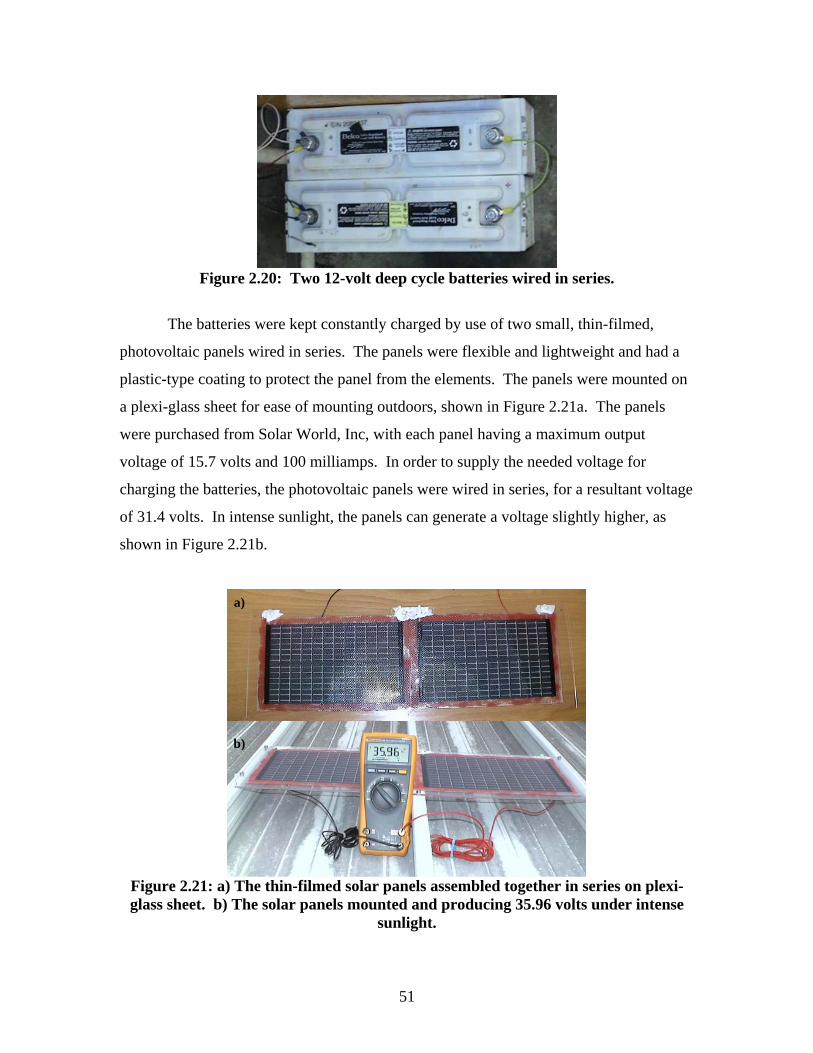
51
Figure 2.20: Two 12-volt deep cycle batteries wired in series.
The batteries were kept constantly charged by use of two small, thin-filmed,
photovoltaic panels wired in series. The panels were flexible and lightweight and had a
plastic-type coating to protect the panel from the elements. The panels were mounted on
a plexi-glass sheet for ease of mounting outdoors, shown in Figure 2.21a. The panels
were purchased from Solar World, Inc, with each panel having a maximum output
voltage of 15.7 volts and 100 milliamps. In order to supply the needed voltage for
charging the batteries, the photovoltaic panels were wired in series, for a resultant voltage
of 31.4 volts. In intense sunlight, the panels can generate a voltage slightly higher, as
shown in Figure 2.21b.
Figure 2.21: a) The thin-filmed solar panels assembled together in series on plexi-glass sheet. b) The solar panels mounted and producing 35.96 volts under intense
sunlight.
a)
b)
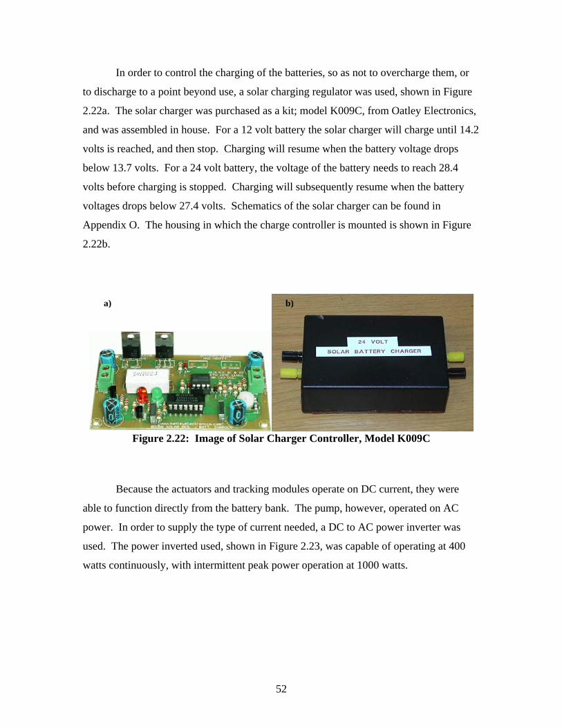
52
In order to control the charging of the batteries, so as not to overcharge them, or
to discharge to a point beyond use, a solar charging regulator was used, shown in Figure
2.22a. The solar charger was purchased as a kit; model K009C, from Oatley Electronics,
and was assembled in house. For a 12 volt battery the solar charger will charge until 14.2
volts is reached, and then stop. Charging will resume when the battery voltage drops
below 13.7 volts. For a 24 volt battery, the voltage of the battery needs to reach 28.4
volts before charging is stopped. Charging will subsequently resume when the battery
voltages drops below 27.4 volts. Schematics of the solar charger can be found in
Appendix O. The housing in which the charge controller is mounted is shown in Figure
2.22b.
Figure 2.22: Image of Solar Charger Controller, Model K009C
Because the actuators and tracking modules operate on DC current, they were
able to function directly from the battery bank. The pump, however, operated on AC
power. In order to supply the type of current needed, a DC to AC power inverter was
used. The power inverted used, shown in Figure 2.23, was capable of operating at 400
watts continuously, with intermittent peak power operation at 1000 watts.
a) b)

53
Figure 2.23: 400 Watt DC to AC Power Inverter
2.11 Generator/Alternator
In order to produce electrical power from the system, a generator has to be
coupled with the output shaft of the steam turbine, Figure 2.26. The generator used was a
443541-10Amp Permanent Magnet DC Generator from Windestream Power LLC. The
generator is capable of producing power at speeds ranging from 0 to 5000 rpm at voltages
between 12 and 48 volts. Maximum power production for this particular generator, for
12, 24, and 48 volts is 120, 240, and 480 watts, respectively. Figure 2.24 shows an image
and Figure 2.25 shows the performance curves for the generator of mention. The
schematics for the generator can be found in Appendix P.
Figure 2.24: Windstream Power 10 Amp Permanent Magnet DC Generator.
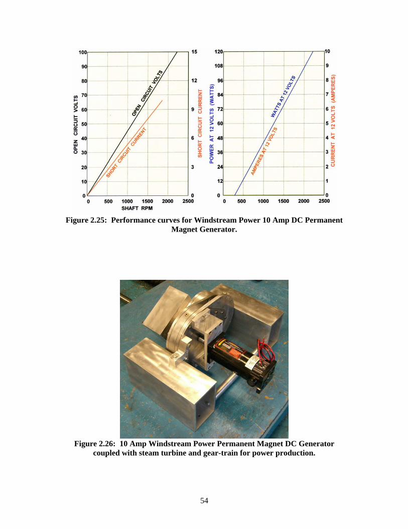
54
Figure 2.25: Performance curves for Windstream Power 10 Amp DC Permanent
Magnet Generator.
Figure 2.26: 10 Amp Windstream Power Permanent Magnet DC Generator
coupled with steam turbine and gear-train for power production.
55
CHAPTER 3
ANALYSIS / RESULTS AND DISCUSSION
3.1 Introduction
This chapter contains a detailed description of the analysis and results which were
obtained for the different components of the concentrating solar thermal system. The
chapter starts with an overview of the solar calculations needed for the solar concentrator
to track the sun. An analysis of the solar concentrator will then be discussed comparing
the expected amount of collected solar radiation and achievable temperature to actual
values. Following is a discussion on the remaining components of the system, including
the receiver, the turbine, and the generator. The chapter is concluded by discussing the
overall efficiency of the system.
3.2 Solar Calculations
For the solar concentrator to track the sun, and to determine the efficiency of the
concentrator, the amount of solar radiation incident on the collector and the position of
the sun ‘relative’ to the location of the collector (the Ptolemaic view) was needed. The
location of the solar collector is Tallahassee, Florida with Latitude of 30.38° North,
Longitude of 84.37° West, and a Standard Time Meridian of 75° West. For
simplification, the calculations in this section are performed for a single day, October 12th
(n is equal to 285), at solar noon, in which the hour angle is at 0 degrees. Full
calculations for the particular day mentioned and for the range of the entire year are
available in Appendicies B and C.
As was discussed in the section of Solar Geometry from Chapter 1, the solar
declination angle, the angle between the earth-sun line and the plane through the equator
(refer to Figure 1.6), is needed to perform calculations for the position of the sun. The
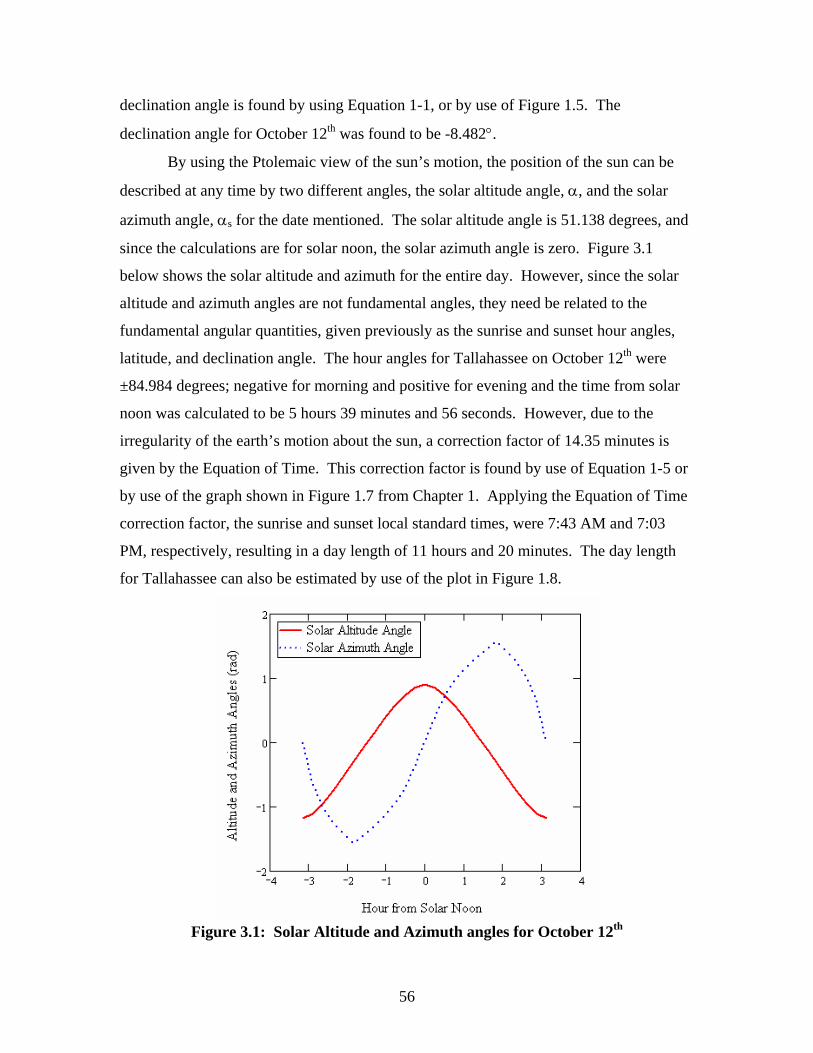
56
declination angle is found by using Equation 1-1, or by use of Figure 1.5. The
declination angle for October 12th was found to be -8.482°.
By using the Ptolemaic view of the sun’s motion, the position of the sun can be
described at any time by two different angles, the solar altitude angle, α, and the solar
azimuth angle, αs for the date mentioned. The solar altitude angle is 51.138 degrees, and
since the calculations are for solar noon, the solar azimuth angle is zero. Figure 3.1
below shows the solar altitude and azimuth for the entire day. However, since the solar
altitude and azimuth angles are not fundamental angles, they need be related to the
fundamental angular quantities, given previously as the sunrise and sunset hour angles,
latitude, and declination angle. The hour angles for Tallahassee on October 12th were
±84.984 degrees; negative for morning and positive for evening and the time from solar
noon was calculated to be 5 hours 39 minutes and 56 seconds. However, due to the
irregularity of the earth’s motion about the sun, a correction factor of 14.35 minutes is
given by the Equation of Time. This correction factor is found by use of Equation 1-5 or
by use of the graph shown in Figure 1.7 from Chapter 1. Applying the Equation of Time
correction factor, the sunrise and sunset local standard times, were 7:43 AM and 7:03
PM, respectively, resulting in a day length of 11 hours and 20 minutes. The day length
for Tallahassee can also be estimated by use of the plot in Figure 1.8.
Figure 3.1: Solar Altitude and Azimuth angles for October 12th

57
By having a collector which follows the position of the sun, an optimum amount of solar
radiation can be collected. At solar noon, the total instantaneous solar radiation falling on
the parabolic concentrator was found to be approximately 1.15 kW/m2. However, only
beam (direct) insolation can be utilized due to the type of collector used. This results in
approximately 1.064 kW/m2 of solar radiation. The calculations for how these values
were obtained are located in Appendix E. Figure 3.2, below, shows a comparison of the
total instantaneous and beam solar insolation falling on the collector in Tallahassee, FL.
Figure 3.2: Comparison of the Total Insolation available to that of the Beam Insolation falling on the SESEC solar collector located in Tallahassee, FL.
3.2 Analysis of the Dish
Measurements of the dish were taken to calculate the equation to describe the
shape of it. The dish is considered to be that of a parabolic concentrator with a diameter

58
of 3.66 meters (144 inches), and a depth of 0.648 meters (25.5 inches). The surface area
of the dish is thus calculated by the following equation:
Aconcentrator =2 ⋅ π3 ⋅ P
⋅D2
4+ P 2
⎛
⎝ ⎜
⎞
⎠ ⎟
3
− P 3⎡
⎣
⎢ ⎢
⎤
⎦
⎥⎥ (3-1)
where
P =D2
8 ⋅ H (3-2)
The resulting surface area of the concentrator is 11.73 m2 (126.28 ft2). The cross-section
of the concentrator can be viewed as a parabola, which is given by the equation
f (x) = a ⋅ x 2 + b (3-3)
where f(x) is the function describing the shape of the parabola, x is the horizontal distance
from the center, and the constants a and b describe the shape of the parabola. b can be
made zero by placing the bottom center of the concentrator at the origin. From this
constraint, the value of f(x) is equal to the depth when x is equal to the radius of the dish.
Thus, the constant a can be calculated using the following equation:
a =Depth
Radius2 (3-4)
This constant is found to be 0.194 per meter (0.004919 per inch) and is used to determine
the focal length of the collector. The focal length of the concentrator is defined as the
distance from the bottom of the parabola to the concentration point (focal point). For a
symmetric parabola, the focal point lies along the axis of symmetry where the distance
above the intersection of the axis and curve gives the focal length by
59
focal _ length =1
4 ⋅ a (3-5)
thus establishing where there focal point is located relative to the bottom of the
concentrator.
The calculation of the focal length is useful for positioning of the receiver,
however, due to the dynamics involving the sun, earth, and optics of the concentrator, the
focal point will not be an exact point, but will actually be more of a focal area. The area
in which the radiation is condensed determines the radiation intensity. The higher the
intensity, the higher the temperature that the receiver can attain.
In order to calculate the maximum achievable temperature of the concentrator, the
geometric concentration ratio needs to be determined. By convention, the receiver at the
focal area would be considered as a flat plate absorber, thus the area that would be used
for calculation of the concentration ratio would be the flat circular bottom region of the
receiver. However, the receiver of the solar thermal system discussed here is
‘submerged’ in the focal region, thus more surface area of the absorber is receiving the
concentrated solar radiation. The area of the receiver is calculated to be 0.109 m2, with
the aperture area of the concentrator being 10.507 m2, resulting in a geometric
concentration ratio of 96. By using the standard assumptions given by Rabb , the
transmissivity,τ, is equal to 0.5, the absorptance of the receiver, α, is 0.7, and the
emmittance of the receiver in the infrared region, ε, is 0.5; the radiation transfer from the
sun to the receiver is calculated as follows:
42 )(sin sunhalforconcentratreceiversun TAQ σθτα=→ (3-6)
where the half-angle of the sun, θhalf, is found to be 0.266° by use of
earthsun
sunhalf R
r
→
=θ (3-7)

60
where kmrsun 695500= and kmR earthsun8104967.1 ×=→ . The ideal concentration ratio
can then be determined using:
)(sin1
2half
idealCRθ
= (3-8)
which results in 46310=idealCR . These values can now be used in the following
equation to calculate the maximum achievable temperature of the concentrator for the
geometric concentration ratio of the system:
41
)1( ⎥⎦
⎤⎢⎣
⎡−=
ideal
geometricsunreceiver CR
CRTT
εατη (3-9)
From Equation 3-9, the maximum achievable temperature of the receiver, Treceiver, was
found to be to be 984.732 K (1313°F). The calculations for the theoretical maximum
temperature of the collector can be located in Appendix G. Experimentally, the
maximum internal temperature of the receiver was approximately 834.15 K (1041°F) and
the external temperature was 922 K (1200°F). It is assumed that this discrepancy is due
to the assumed values for the transmissivity, absorbtivity, and emmittance of the dish, as
well as the degradation of the reflective surface and the solar intensity of the day. In
Figure 3.3, it is shown how the receiver temperature relates to the geometric
concentration ratio of the system. The figure also shows how the concentrator discussed
in this work is less efficient than ideal.

61
Figure 3.3: Relationship between the concentration ratio and the receiver operation
temperature.
3.3.1 Efficiency of Collector
A solar concentrator is more efficient at high temperatures in that it reduces the
area from which heat is lost. In order to calculate the efficiency of the concentrating
collector, the absorbed radiation per unit area of aperture must be estimated from the
radiation and the optical characteristics of the concentrator and receiver (Duffie). A
simple energy balance equation yields the useful energy delivered by the collector to the
receiver as
rambrLaboout ATTUAIQ )( −−= η (3-10)
The energy balance equation can be rearranged to yield the instantaneous efficiency of a
solar thermal collector, which is defined as the ratio of the useful energy delivered to the
total incoming solar energy. The following equation shows this relation
( )b
arL
amb
ro
ba
outcollector I
TTUAA
IAQ −
−== ηη (3-11)

62
In order to calculate the efficiency of the concentrating collector, the absorbed radiation
per unit area of aperture must be estimated from the radiation and the optical
characteristics of the concentrator and receiver. This is given by Qout, which is defined as
lossoptout QQQ −= (3-12)
where Qopt is the rate of the optical energy absorbed by the receiver, and Qloss is the rate
of the energy lost from the receiver to the ambience. The optical energy that is absorbed
by the receiver from the concentrating collector is defined by the following (Duffie)
bgmsaopt SIAQ γατρ _= (3-13)
The terms in this equation depend upon the geometry and parameters of the receiver and
the collector. Where S is the receiver shading factor, αr is the absorbtance of the receiver,
ρs_m is the specular reflectance of the concentrator, and τg is the transmittance of the glass
envelope over the receiver (if one is present), Aa is the aperture area of the collector, and
Ib is the beam insolation incident on the collector aperture. The terms S, αr, ρs_m, and τg
are constants which are dependent on the materials used and the accuracy of the collector,
and are nominally lumped into a single constant term, known as the optical efficiency of
the collector, ηopt. The rate of optical energy absorbed by the receiver, Qopt, was
calculated to be 11.072 kW.
The thermal energy lost from the receiver, Qloss, to the ambient surroundings is
described by
)( ambrLrloss TTUAQ −= (3-14)
where Ar is the surface area of the receiver, UL is the overall heat loss coefficient, Ta is
the ambient temperature, and Tr is the averaged receiver temperature. Tr is represented
by the following equation
63
2inout
rTT
T+
= (3-15)
where Tout, the temperature of the fluid exiting the receiver was 922 K, and Tin, the
temperature of the fluid entering the receiver was 305 K. The resultant averaged receiver
temperature was then calculated to be 613.5 K. The heat loss coefficient, UL, however, is
not a simple constant, but instead, varies as heat-loss mechanisms change with
temperature. For example, as the temperature increases, the radiant heat loss from the
receiver increases. For computation of the heat loss coefficient, it is assumed that there
are no temperature gradients about the receiver and that there are no losses through
conduction between the receiver and its supporting structure. The heat loss coefficient,
UL, for the receiver type discussed in this work is given as
1
,,
1)(
−
−− ⎥⎥⎦
⎤
⎢⎢⎣
⎡+
+=
crrcacrw
rL hAhh
AU (3-16)
where hw is given as the convective coefficient, hr,c-a is the radiation coefficient between
the receiver (or glass cover) and the ambient, hr,r-c is the radiation coefficient between the
receiver and the glass cover (if there is a cover), Ar is the surface area of the receiver, and
Ac is the surface area of the glass cover (if one is used). Since the receiver used in this
work does not utilize a glass cover, Equation 3-16 is simplified to
1
1−
⎥⎦
⎤⎢⎣
⎡+
=rw
L hhU (3-17)
The linearized radiation coefficient can thus be calculated by (Duffie)
34 meanr Th σε= (3-18)
64
where σ is the Stefan-Boltzmann constant, ε is the emittance of the absorbing surface, and
Tmean is the mean temperature for radiation. The emittance had a value of 0.5 with the
mean temperature being the same as the inlet water temperature, at 305 K. The radiation
coefficient was calculated to be 3.218 W/m2-K.
The convective heat loss coefficient, hw, is modeled and solved as flow of air
across a cylinder in an outdoor environment. The equations recommended by McAdams
(Duffie) have been modified to account for the outdoor conditions by increasing the
original coefficients by 25 percent. The Nusselt number is thus given as
52.0Re54.040.0 +=Nu (3-19)
for Reynolds numbers which fall between 0.1 and 1000, and as
6.0Re30.0=Nu (3-20)
for Reynolds numbers between 1000 and 50000. For the calculations presented in this
section, a wind speed of 0.5 m/s is assumed. The Reynolds number was calculated to be
1476 by use of Equation 3-21,
νouterDV ⋅
=Re (3-21)
where V is the wind speed, Douter is the diameter of the receiver, and ν is the viscosity,
with a value of sec5 21015.5 m−⋅ . The Reynolds number was then used in conjunction with
Equation 3-20, yielding a Nusselt number of 23.907. The convection coefficient was
then calculated by using Equation 3-22, to obtain a value of 7.172 W/m2-K.
NuDk
houter
airw ⋅= (3-22)

65
The radiation coefficient and convection coefficient are then used with Equation
3-17, yielding a heat loss coefficient value of 10.39 W/m2-K. The heat loss coefficient,
UL is then used in Equation 3-14 to solve for Qloss, yielding a value of 384.42 Watts for
the averaged receiver temperature. As was mentioned previously, the heat loss from the
receiver increases as the operating temperature increases. Figure 3.4 illustrates the linear
trend of the heat loss from the receiver along with the energy loss of the receiver at the
averaged outlet temperature at steady-flow of 367 K.
Figure 3.4: Heat loss from receiver as function of receiver temperature.
Substituting the obtained values of 11.072 kW and 384.42 Watts, for Qopt and Qloss,
respectively, into Equation 3-12, the thermal output value of 10.68 kW was obtained.
This is the amount of thermal energy that was being transferred from the concentrator to
the receiver, which results in a collector efficiency of 95.56 percent. Figure 3.5 shows
the collector efficiency for various receiver temperatures.

66
Figure 3.5: Experimental collector efficiency over a range of values of (Ti – Tamb)/Ib.
3.4 Receiver
The next component of the solar thermal system to be characterized was the
receiver, which acts as a boiler in a traditional Rankine cycle. Even though the receiver
uses an integrated latent heat storage system, it was still subject to convective and
radiation losses, as was described in the previous section. Two options were available to
combat these losses; insulate the receiver or use an insulated cavity/cone allowing for the
receiver to resemble that of a cavity type receiver. A comparison test was performed to
determine which method of insulation would be optimal. For repeatability and
consistency in the initial tests, a 1650 Watt electric burner was used for heating the
receiver. As shown in Figure 3.6, it was found that an uninsulated receiver was only
capable of achieving a temperature of 500 K, and would rapidly cool to 300 K in 40
minutes. The insulated cone allowed for a small increase in initial heating, up to 550 K,

67
and added longevity to the contained heat. Initially, with the insulated cone, the receiver
would decrease by 100 K in the first four minutes, then slowly cool to 300 K in the
following 90 minutes. When the receiver was insulated directly, it reached a maximum
temperature of 700 K on the electric burner. Allowing the insulated receiver to cool, it
reached 500 K in 18 minutes where it plateaued for five minutes, then began to cool
again. From this plateau point, it took the insulated receiver 95 minutes to reach 300 K.
In Figure 3.6 it can be seen that each of the three cases plateau around 500 K. This
plateau is due to the draw salt mixture undergoing a phase change from a molten state
back to a solid form.
300
350
400
450
500
550
600
650
700
0 20 40 60 80 100 120
Time (minutes)
Tem
pera
ture
(K)
No Insulation (K)
Insulated (K)
Insulated Cone (K)
Region of Phase-Change of the Draw Salt (~500 K)
Figure 3.6: Transient Cooling of Thermal Bath at Room Temperature (~298 K)
Although the insulated cone allowed for a greater surface area of the receiver to attain the
concentrated solar radiation, it permitted too great of heat transfer from the receiver to its
surroundings. Thus, from these series of initial tests, it was concluded that it was best to
insulate this particular receiver directly.
68
Once the method of insulation of the receiver was decided upon and the latent
heat storage was characterized, the receiver was then placed at the focal point of the
parabolic concentrator. The receiver was first subjected to a continuous heat addition
test. This allowed for the experimental determination of the maximum possible
temperature that the receiver could reach internally, thus giving a comparison to the
theoretical maximum achievable temperature of the concentrator. As was mentioned
earlier, the receiver was found to have reached a maximum temperature of 834.15 K
(1041 °F), whereas the calculated maximum theoretical temperature was found to be
984.73 K (1313 °F).
In order to better characterize the receiver, a steady-flow experiment was
performed. The receiver was left as an open system, and a flow-rate of 1.0 liter per
minute of water, at an average inlet temperature of 300 K, was pumped through the
receiver for five days. Figure 3.7 and Figure 3.8 show the thermal profiles for the
receiver along with the inlet and outlet water temperatures, and the energy profile for the
various days, respectively. Because of the heat transfer to the water, it was found that the
receiver would only reach a fraction of the maximum achievable temperature. Also, in
Figure 3.7, it shows that there is a maximum temperature that the water is capable of
reaching in this steady-flow experiment, even as the temperature of the receiver
increases, which is most likely due to the design of the receiver. Examination of the
profiles reveals that the temperature of the system would vary due to the slightest cloud
cover or variance in the tracking. The water exiting the receiver reached an average
temperature of 310.6 K; which was insufficient for reaching the phase-change state of
water. For this particular test, other flow rates were not utilized because of flow-rate
limitations dictated by the pump being used, with 1.0 LPM being the lowest flow-rate of
the particular pump, and since steam production was the goal of the system, a higher
flow-rate would be of no use. Thus, for steady-flow characterization of the receiver, a
flow-rate of 1.0 LPM was used.

69
300
350
400
450
500
0 30 60 90 120 150 180 210 240
Time (minutes)
Tem
pera
ture
(K)
7/17/06 - Thermal Bath Temp 7/17/06 - Exit Temp
7/18/06 - Thermal Bath Temp 7/18/06 - Exit Temp
7/19/06 - Thermal Bath Temp 7/19/06 - Exit Temp
7/20/06 - Thermal Bath Temp 7/20/06 - Exit Temp
7/21/06 - Thermal Bath Temp 7/21/06 - Exit Temp
Figure 3.7: Temperature Profile for steady-flow tests at 1.0 LPM. Test performed
for week of July 17 through July 21, 2006. Average inlet temperature of 300 K. Plot shows thermal draw salt bath temperature and exit water temperature.
0
200
400
600
800
1000
1200
1400
0 30 60 90 120 150 180 210 240
Time (minutes)
Q_d
ot (W
atts
)
7/17/2006 7/18/2006 7/19/2006 7/20/2006 7/21/2006 Figure 3.8: Usable energy (Q) in Watts for extended period of time over a period of
five days. Date of 7/20/06 was perfectly clear skies. Other days had intermittent cloud cover, showers, or were overcast.

70
It was realized that an intense amount of energy would be required to generate a constant
flow of steam from the receiver. As this system would be incapable of maintaining this
amount of energy, it was decided to operate the system intermittently. The receiver was
allowed to heat to a maximum temperature before water was pumped into the receiver
where it would instantly flash to steam. The water flow would be terminated when the
thermal bath of the receiver reached a minimum temperature. The system was then
allowed to reheat to the maximum temperature and the cycle was repeated. The
experiments performed for the intermitent system set the duty cycle, flow-rate, and
maximum and minimum operating temperatures.
For the first set of tests, the receiver was heated by the concentrator to a
temperature around 500 K. The pump was then turned on, and throttled back by use of a
needle valve, to a flow-rate of 0.734 LPM. The water entering the receiver was at a
temperature of 300 K before it was flashed to steam with an exit temperature of 450 K.
In order to determine which flow rate would be best for overcoming the back pressure
created by the steam, this test was repeated for the following flow rates: 1.36 LPM, 1.67
LPM, and 2.054 LPM, to determine which flow rate would be best for overcoming the
back pressure created by the steam. Figure 3.9 shows the comparison of the inlet, exit,
and thermal bath temperatures for the flow-rates mentioned. It was found that a flow rate
below 1.0 LPM was not enough to overcome the back pressure created by the steam to
keep a flow of feed-water into the boiler, but a flow above 1.0 LPM was sufficient, as
shown in Figures 3.10 and 3.11 for the flow rates of 0.734 LPM and 1.36 LPM,
respectively. Figures 3.11 and 3.12 demonstrate repeatability of the experiments
performed on different days. By comparison of the data between the various flow rates,
and by hardware dictation, it was found that the minimum flow-rate of 1.0 LPM was
optimum for steam production in our system because of the extended run time that it
allowed. The system loop was closed with the addition of the steam turbine.

71
300
350
400
450
500
550
0 1 2 3 4 5 6
Time (minutes)
Tem
pera
ture
(K)
0.734 LPM -- Thermal Bath 0.734 LPM -- Outlet 1.36 LPM -- Thermal Bath1.36 LPM -- Outlet 1.67 LPM -- Thermal Bath 1.67 LPM -- Outlet2.054 LPM -- Thermal Bath 2.054 LPM -- Outlet
Figure 3.9: Various flow rate tests for steam flashing.
300
350
400
450
500
550
600
650
700
750
0 5 10 15 20 25
Time (minutes)
Tem
pera
ture
(K)
0
1
2
3
4
5
6
7
8
Pres
sure
(PSI
G)
Thermal Bath Temp (K) Inlet Water Temp (K) Steam Temp (K) Boiler Steam Exit Pressure (PSIG) Figure 3.10: Temperature and Pressure profile for flash steam with feed water at
flow rate of 0.734 LPM.

72
300
350
400
450
500
550
600
650
700
750
0 0.5 1 1.5 2 2.5 3 3.5 4
Time (minutes)
Tem
pera
ture
(K)
0
10
20
30
40
50
60
70
80
Pres
sure
(PSI
G)
Thermal Bath Temp (K) Inlet Water Temp (K) Steam Temp (K) Boiler Steam Exit Pressure (PSIG) Figure 3.11: Temperature and Pressure profile for flash steam with feed water at
flow rate of 1.36 LPM (Test 1)
300
350
400
450
500
550
600
650
700
750
0 0.5 1 1.5 2 2.5 3 3.5 4
Time (minutes)
Tem
pera
ture
(K)
0
10
20
30
40
50
60
70
80
Pres
sure
(PSI
G)
Thermal Bath Temp (K) Inlet Water Temp (K) Steam Temp (K) Boiler Steam Exit Pressure (PSIG) Figure 3.12: Temperature and Pressure profile for flash steam with feed water at
flow rate of 1.36 LPM (Test 2). Comparable to Figure 3.11.

73
The first set of experiments performed with the system closed and turbine in place at a
flow rate of 1.0 LPM was to determine the minimum and maximum operating
temperature of the receiver. This was done to determine when to operate the pump. As
was observed in previous tests, it was inadequate to operate the system while the thermal
bath of the receiver was below a temperature of 533 K (500°F), which is the temperature
at which the phase change of the salt occurs. Thus, the initial tests were run by heating
the receiver to a temperature of 588.71 K (600°F). Once the operating temperature was
reached, the pump was turned on and the water was flashed to steam, with the
temperatures and pressures measured at strategic points in the system, as mentioned in
section 8.2. The initial heating of the receiver took the longest due to the phase-change
which the draw salt must undergo. Water was pumped into the receiver until the thermal
bath reached a temperature of 533 K, at which point the pump was turned off. The
receiver was then heated to a temperature of 644.26 K (700°F) and the process repeated.
The experimental process was repeated at 100°F intervals until a maximum temperature
of 810.93 K (1000°F) was achieved. Run time and receiver heating time was recorded
along with the temperatures and pressures at the various points in the system.
Because the system is unable to generate enough energy to power a turbine continuously,
the system is run intermittently. The previously mentioned tests determined the start up
and shut down temperatures of 600 K and 700 K, for which the intermittent cycles will
operate. Testing of the closed system was then continued to assure repeatability of
results. Figure 3.13 shows a typical run cycle for 150 minutes, with a total of three runs.
Figure 3.14 shows a closer inspection for the initial heating of this particular test. It
clearly illustrates where the phase change of the draw salt occurs, between the 20 and 25
minute mark. This is the point where the draw salt changes from solid to a completely
molten solution.

74
300
350
400
450
500
550
600
650
700
750
800
0 50 100 150 200 250
Time (minutes)
Tem
pera
ture
(K)
Thermal Bath Temp (K) Receiver Inlet Temp (K) Steam Temp (K)Turbine Inlet Temp (K) Turbine Exit Temp (K) Reservoir Water Temp (K)
45 minutes for reheat
35 minutes for reheat
54 minutes to reach temperature initially
700 K (816 deg F)720 K (836 deg F)
715 K (827 deg F)
530 K (430 deg F)555 K (475 deg F)
569 K (500 deg F)
Figure 3.13: Plot of temperature profiles for the thermal bath, receiver inlet,
receiver exit, turbine inlet, turbine exit, and the water supply/return reservoir. Shows repeatability of three runs in 150 minutes.
295
345
395
445
495
545
595
645
695
745
0 10 20 30 40 50
Time (minutes)
Tem
pera
ture
(K)
Thermal Bath Temp (K) Receiver Inlet Temp (K) Steam Temp (K)Turbine Inlet Temp (K) Turbine Exit Temp (K) Reservoir Water Temp (K)
~700K
Phase Change of the Draw Salt (from solid to liquid)
Figure 3.14: Initial heating of system from ambient to operating temperature of 700
K in 54 minutes. Shows phase change of the draw salt used in the thermal bath.

75
The following figure, Figure 3.15, shows a closer view of the thermal profile of the
system further down the time line during the first run of the system. In this figure it is
noticeable that there is a 175 K temperature drop of the steam between the exit of the
receiver and the inlet of the turbine. This temperature drop is due to line losses from the
long run from the boiler to the turbine and due to the line not being insulated, allowing
for radiation of energy to the surroundings.
295
345
395
445
495
545
595
645
695
745
54 55 56 57 58 59 60 61 62 63 64 65 66 67
Time (minutes)
Tem
pera
ture
(K)
Thermal Bath Temp (K) Receiver Inlet Temp (K) Steam Temp (K)Turbine Inlet Temp (K) Turbine Exit Temp (K) Reservoir Water Temp (K)
Heat LossdT=175 K
Expansion through turbine
600 K
425 K
Figure 3.15: Run one of multiple tests for October 12th. Plot shows temperature drop in system as the steam is expanded through the turbine and the temperature
drop of 175 K between the exit of the boiler and the inlet of the turbine.
Through the intermittent operation, the receiver is able to produce an average of 8.11 kW
of usable thermal energy, with an instantaneous spike of 23.4 kW from when water first
enters the boiler. This 23.4 kW spike of thermal energy is due to the instantaneous
release of the stored energy from the latent heat storage of the receiver to the water,
resulting in the production of superheated steam. Figure 3.16 shows the available
thermal energy from the receiver for the set of three runs on October 12th. It was
determined that the steam turbine had an average run time of 2.5 minutes for each of its
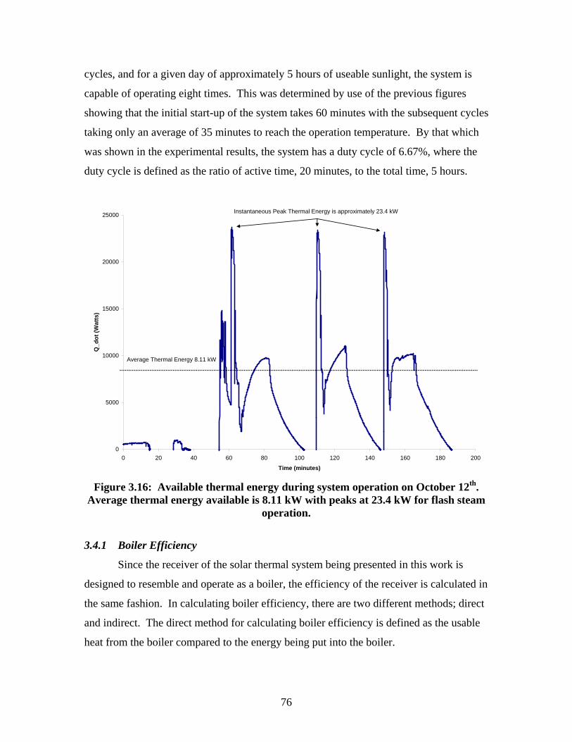
76
cycles, and for a given day of approximately 5 hours of useable sunlight, the system is
capable of operating eight times. This was determined by use of the previous figures
showing that the initial start-up of the system takes 60 minutes with the subsequent cycles
taking only an average of 35 minutes to reach the operation temperature. By that which
was shown in the experimental results, the system has a duty cycle of 6.67%, where the
duty cycle is defined as the ratio of active time, 20 minutes, to the total time, 5 hours.
0
5000
10000
15000
20000
25000
0 20 40 60 80 100 120 140 160 180 200
Time (minutes)
Q_d
ot (W
atts
)
Instantaneous Peak Thermal Energy is approximately 23.4 kW
Average Thermal Energy 8.11 kW
Figure 3.16: Available thermal energy during system operation on October 12th.
Average thermal energy available is 8.11 kW with peaks at 23.4 kW for flash steam operation.
3.4.1 Boiler Efficiency
Since the receiver of the solar thermal system being presented in this work is
designed to resemble and operate as a boiler, the efficiency of the receiver is calculated in
the same fashion. In calculating boiler efficiency, there are two different methods; direct
and indirect. The direct method for calculating boiler efficiency is defined as the usable
heat from the boiler compared to the energy being put into the boiler.

77
input
outputboiler Q
Q=η (3-23)
For steady flow through the boiler, Qoutput, the usable heat output from the boiler, was
found to be approximately 1 kW, and the power input of the boiler, Qinput, was 11.072 kW.
By the direct method for determining boiler efficiency, the boiler was calculated to be
9.032 percent efficient. The indirect method, on the other hand, determines the boiler
efficiency by the sum of the major losses from the boiler to the energy input of the boiler
and is defined as
input
lossesindirectboiler Q
Q−= 1_η (3-24)
where the sum of the major losses, Qlosses, was determined to be 349.37 Watts. This
results in a boiler efficiency of about 96.85 percent. Although the indirect method for
determining boiler efficiency provides a better understanding of how the losses effect the
efficiency, it does not take in account other losses internally in the boiler. Thus, for this
work, the boiler efficiency of 9.032 percent, calculated by the direct method, will be used
because it is an actual comparison of the usable thermal energy to that of the energy input
into the boiler. (Helsinki University, Sebastian Teir, Antto Kulla)
3.5 Turbine Efficiency
As the turbine that was used was an impulse turbine, it was already known that it
would have a lower efficiency than the multistage turbines used in more advanced power
systems. Short-term transient start-up or shutdown of the turbine will not be included for
the calculations, only the steady operating period of time. In order to model the turbine
for calculation purposes, it was assumed that the process through the turbine was a
steady-state, steady-flow process.

78
The mass flow of steam into the turbine was first solved for by using the turbine
inlet pressure and temperature of 480.537 kPa and 431.46 K, respectively. The steam
turbine had a nozzle diameter of 0.229 cm and is modeled as that of a free jet. The flow
was found to be choked, with Pexit / Pturbine being equal to 0.211. The mass flow rate of
steam through the nozzle into the turbine was then calculated to be skg /10873.4 3−× .
The full calculations for the mass flow rate of the steam into the turbine are located in
Appendix J.
The heat transfer from the turbine,Q& , was calculated to be 410.871 Watts with the
work from the turbine being 650.818 Watts by use of Equation 1-44. In order to
determine the efficiency of the turbine, however, it must be compared to the theoretical
performance of the same turbine under ideal conditions. The ideal process for a steam
turbine is considered to be a reversible adiabatic process between the inlet state of the
turbine and its exhaust pressure. Thus, by comparing the turbine discussed in this work,
under its actual operating conditions, to that of the same steam turbine under ideal
conditions, we find that our steam turbine has a thermal efficiency of 49.98 percent. The
full calculations for this are found in Appendix K.
3.6 Turbine/Gear-Train Analysis
With the gear-train attached to the steam turbine, tests were performed to determine the
resulting shaft (mechanical) power of the gear train. The tests were performed by use of
a Prony Brake with a 152.4 mm (6 in) diameter flywheel coupled to the output shaft of
the gear-train with the turbine inlet at a steam pressure of 344.74 kPa. It was found that
on average, the output shaft power of the turbine/gear-train was approximately 1.34 kW
with an average shaft speed of 300 RPM. Table 3.1 shows the results from the tests,
yielding shaft speed, torque, and shaft power.
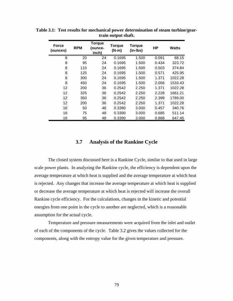
79
Table 3.1: Test results for mechanical power determination of steam turbine/gear-train output shaft.
Force (ounces) RPM
Torque (ounce-
inch)
Torque (N-m)
Torque (in-lbs) HP Watts
8 20 24 0.1695 1.500 0.091 68.158 95 24 0.1695 1.500 0.434 323.728 110 24 0.1695 1.500 0.503 374.848 125 24 0.1695 1.500 0.571 425.958 300 24 0.1695 1.500 1.371 1022.288 450 24 0.1695 1.500 2.056 1533.43
12 200 36 0.2542 2.250 1.371 1022.2812 325 36 0.2542 2.250 2.228 1661.2112 350 36 0.2542 2.250 2.399 1789.0012 200 36 0.2542 2.250 1.371 1022.2816 50 48 0.3390 3.000 0.457 340.7616 75 48 0.3390 3.000 0.685 511.1416 95 48 0.3390 3.000 0.868 647.45
3.7 Analysis of the Rankine Cycle
The closed system discussed here is a Rankine Cycle, similar to that used in large
scale power plants. In analyzing the Rankine cycle, the efficiency is dependent upon the
average temperature at which heat is supplied and the average temperature at which heat
is rejected. Any changes that increase the average temperature at which heat is supplied
or decrease the average temperature at which heat is rejected will increase the overall
Rankine cycle efficiency. For the calculations, changes in the kinetic and potential
energies from one point in the cycle to another are neglected, which is a reasonable
assumption for the actual cycle.
Temperature and pressure measurements were acquired from the inlet and outlet
of each of the components of the cycle. Table 3.2 gives the values collected for the
components, along with the entropy value for the given temperature and pressure.
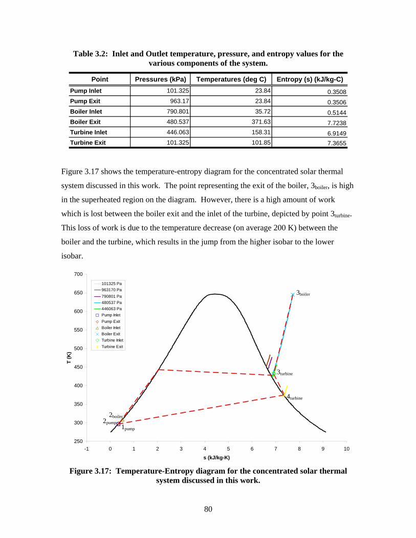
80
Table 3.2: Inlet and Outlet temperature, pressure, and entropy values for the various components of the system.
Point Pressures (kPa) Temperatures (deg C) Entropy (s) (kJ/kg-C)Pump Inlet 101.325 23.84 0.3508Pump Exit 963.17 23.84 0.3506Boiler Inlet 790.801 35.72 0.5144Boiler Exit 480.537 371.63 7.7238Turbine Inlet 446.063 158.31 6.9149Turbine Exit 101.325 101.85 7.3655
Figure 3.17 shows the temperature-entropy diagram for the concentrated solar thermal
system discussed in this work. The point representing the exit of the boiler, 3boiler, is high
in the superheated region on the diagram. However, there is a high amount of work
which is lost between the boiler exit and the inlet of the turbine, depicted by point 3turbine.
This loss of work is due to the temperature decrease (on average 200 K) between the
boiler and the turbine, which results in the jump from the higher isobar to the lower
isobar.
250
300
350
400
450
500
550
600
650
700
-1 0 1 2 3 4 5 6 7 8 9 10
s (kJ/kg-K)
T (K
)
101325 Pa963170 Pa790801 Pa480537 Pa446063 PaPump InletPump Exit Boiler Inlet Boiler ExitTurbine InletTurbine Exit
Figure 3.17: Temperature-Entropy diagram for the concentrated solar thermal
system discussed in this work.
1pump 2pump
2boiler
3boiler
3turbine
4turbine
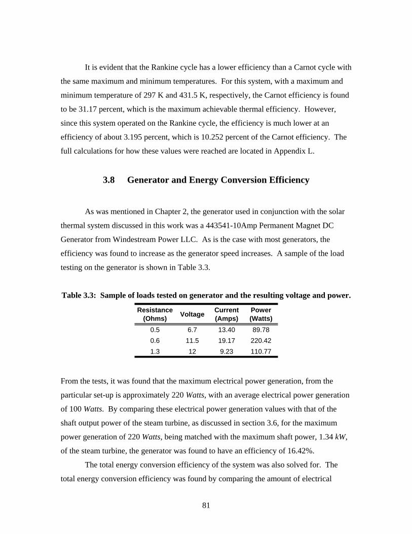
81
It is evident that the Rankine cycle has a lower efficiency than a Carnot cycle with
the same maximum and minimum temperatures. For this system, with a maximum and
minimum temperature of 297 K and 431.5 K, respectively, the Carnot efficiency is found
to be 31.17 percent, which is the maximum achievable thermal efficiency. However,
since this system operated on the Rankine cycle, the efficiency is much lower at an
efficiency of about 3.195 percent, which is 10.252 percent of the Carnot efficiency. The
full calculations for how these values were reached are located in Appendix L.
3.8 Generator and Energy Conversion Efficiency
As was mentioned in Chapter 2, the generator used in conjunction with the solar
thermal system discussed in this work was a 443541-10Amp Permanent Magnet DC
Generator from Windestream Power LLC. As is the case with most generators, the
efficiency was found to increase as the generator speed increases. A sample of the load
testing on the generator is shown in Table 3.3.
Table 3.3: Sample of loads tested on generator and the resulting voltage and power.
Resistance (Ohms) Voltage Current
(Amps)Power (Watts)
0.5 6.7 13.40 89.780.6 11.5 19.17 220.421.3 12 9.23 110.77
From the tests, it was found that the maximum electrical power generation, from the
particular set-up is approximately 220 Watts, with an average electrical power generation
of 100 Watts. By comparing these electrical power generation values with that of the
shaft output power of the steam turbine, as discussed in section 3.6, for the maximum
power generation of 220 Watts, being matched with the maximum shaft power, 1.34 kW,
of the steam turbine, the generator was found to have an efficiency of 16.42%.
The total energy conversion efficiency of the system was also solved for. The
total energy conversion efficiency was found by comparing the amount of electrical

82
power produced to that of the total amount of solar energy being collected. The total
amount of solar energy being collected is equal to the amount of beam solar insolation
incident on the concentrator, which is a total of 11.36 kW. By using Equation 3-25, it
was found that the total energy conversion efficiency of the system, ηconversion, was 1.94%.
InputEnergy Solar OutputPower Electric
=conversionη (3-25)

83
CHAPTER 4
CONCLUSIONS
4.1 Introduction
The main objective of the current work was to construct a concentrating solar
thermal system which utilizes a Rankine cycle for electrical power generation, and
evaluate the overall efficiency of the system. A brief summary of the results obtained
from the work, along with recommendations for future work are given in the following
sections of this chapter.
4.2 Solar Calculations
• When using the Ptolemaic view of the sun, it can be said that the sun
moves along the azimuth at a rate of 15 degrees per hour with solar noon
being based as the time that the sun is positioned exactly due south.
• Because of the characteristics of the concentrating solar collector, only
beam radiation is usable, which on average, is 100 W/m2 less than the total
beam insolation available in Tallahassee, FL.
4.3 Trackers
• Photo-sensing tracking modules for controlling dish position does an
efficient job at visually tracking the sun throughout the day, however, long
periods of cloud cover become problematic for the trackers to keep the
concentrator oriented properly.
84
4.4 Solar Concentrator
• Concentrator has an aperture area of 10.507 m2 and a geometric
concentration ratio of 96.
• Maximum theoretical temperature at focal region of concentrator is
984.732 K (1313ºF).
• Maximum achieved temperature in focal region of concentrator (internal
temperature of receiver) was 834.15 K (1041ºF).
• Energy incident on collector for October 12th (date calculations where
performed for) is approximately 1064 W/m2 which is equivalent to a total
of 11.18 kW.
• Collector (concentrator and receiver) is found to have an efficiency of
approximately 95.56 percent.
4.5 Receiver / Boiler
• Optical energy absorbed by the receiver was found to be approximately
11.068 kW.
• Major losses from the boiler calculated to be 349.37 Watts.
• Direct method of calculating boiler efficiency yields an efficiency of 9.032
percent; indirect method yields 96.85 percent efficiency.
• Boiler not optimized to provide high pressure steam or continuous steam
flow.
85
4.6 Steam Turbine
• Mass flow rate of steam through nozzle in to turbine is skg /10873.4 3−× .
• Efficiency of the steam turbine was calculated to be 49.98 percent for
current operating conditions.
• Steam turbine/gear-train has a mechanical shaft output power of 1.34 kW.
4.7 Generator
• Maximum power production seen was 220 Watts with a load of 0.6-ohms.
• Average power production approximately 100 Watts.
• Turbine Efficiency (Electric Power Output / Mechanical Shaft Power) was
16.42% for the maximum power of 220 Watts.
4.8 Cycle
• Large temperature drop (ΔT = 175 K) between boiler exit and turbine
inlet.
• Carnot efficiency of the system calculated to be 31.17 percent.
• Rankine cycle efficiency of the system is 3.195 percent; 10.252 percent of
the Carnot efficiency.

86
• Energy conversion efficiency from incoming solar energy to electric
energy was 1.94%.
• Overall efficiency ( generatorturbinepumpcollector ηηηη ××× ) was 7.30%.
4.9 Future Work
• Use a more optimized system for tracking, such as a program written in
labVIEW to calculated the position of the sun along with potentiometers
on each axis of the concentrator for live feed back as to where the system
is located.
• Resurface the concentrator. Use a better material for the reflective coating
than aluminized mylar.
• Redesign of the receiver to a cavity type receiver to optimize amount of
energy absorbed and to minimize losses. Also, utilize a different type of
internal boiler design to maximize heat transfer to the working fluid and to
allow for extended periods of operation.
• Along with receiver redesign, optimize receiver support structure and
collector to support weight of receiver with added weight of turbine and
for ease of installation and maintenance of the receiver.
• Relocate turbine to receiver to minimize losses between the boiler and the
receiver.
• Use a turbine with multiple stages to utilize more energy from the steam
before returning to reservoir.

87
• Integrate in control and data acquisition program control for start-up /
shut-down of pump.
• Investigate various steam engines/turbines for optimization for use with
the system discussed in this work.
• Utilize the solar thermal system for tri-generation.
• Design and fabricate new concentrator, possibly out of composite
materials, to make lighter and more durable.

88
APPENDIX A
RABL’S THEOREM
Concentrator
Aabs
R
r
S
Figure A.1: Radiation Transfer from source S through aperture A of concentrator
to absorber Aabs. (Rabl)
In order to prove his theorem, Rabl set up a thought-experiment (shown in Figure
A.1). The experiment is an isotropically radiating sphere of radius r surrounded by a
sphere of radius R which has an aperture of area A that admits light to a concentrator
behind A. The concentrator focuses the light entering through A onto a smaller area Aabs,
corresponding to a theoretical concentration of
absorberltheoretica A
ACR = (A-1)
It is assumed that the concentrator focuses all light entering A within the half-angle, θ, of
the normal to A. If A/R2 is small, the light from the source, S, incident on A, is uniformly
distributed over all angles between 0 andθ, and there is no light from S, outside of θ.
Extraneous radiation is eliminated by assuming black walls at absolute zero temperature.
The procedure is now to calculate the rates of emission of radiant energy by the source
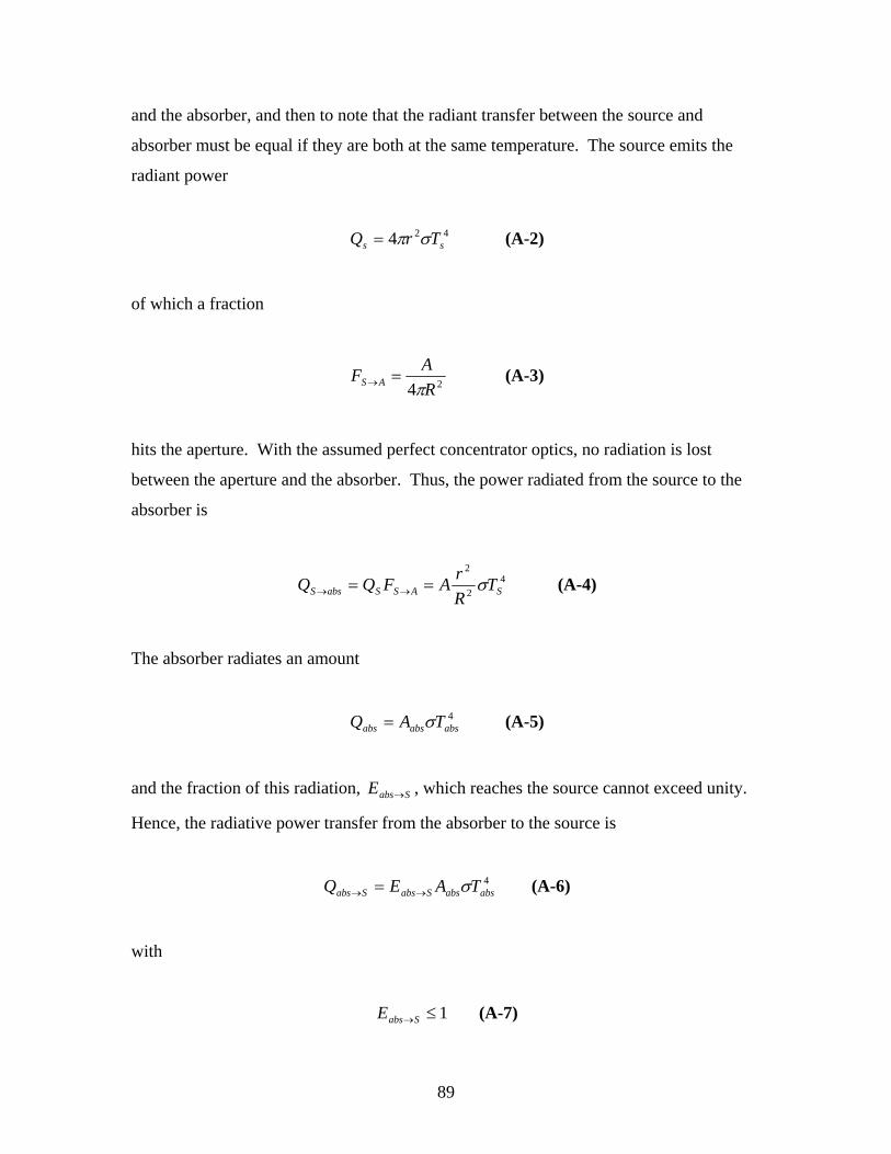
89
and the absorber, and then to note that the radiant transfer between the source and
absorber must be equal if they are both at the same temperature. The source emits the
radiant power
424 ss TrQ σπ= (A-2)
of which a fraction
24 RAF AS π
=→ (A-3)
hits the aperture. With the assumed perfect concentrator optics, no radiation is lost
between the aperture and the absorber. Thus, the power radiated from the source to the
absorber is
42
2
SASSabsS TRrAFQQ σ== →→ (A-4)
The absorber radiates an amount
4
absabsabs TAQ σ= (A-5)
and the fraction of this radiation, SabsE → , which reaches the source cannot exceed unity.
Hence, the radiative power transfer from the absorber to the source is
4
absabsSabsSabs TAEQ σ→→ = (A-6)
with
1≤→SabsE (A-7)

90
If the source and the absorber are at the same temperature, the second law of
thermodynamics requires that there cannot be any net heat transfer between these bodies.
Thus, if we set Sabs TT = , it follows that
SabsabsS QQ →→ = (A-8)
Therefore,
absSabs AERrA →=2
2
(A-9)
from which we deduce that the theoretical concentration satisfies
)(sin 22
2
θSabs
Sabsabs
ltheoreticaE
ErR
AACR →
→ === (A-10)
Since the maximum possible value of SabsE → is unity, the concentration must satisfy
)(sin12 θ
≤ltheoreticaCR (A-11)
For collectors in which the equal sign holds are called ideal collectors.
(Rapp)

91
APPENDIX B
SOLAR ANGLE AND INSOLATION CALCULATIONS
Solar Calculations
Calculations performed for Tallahassee, FL (located in Eastern Time Zone w/Daylight Savings) Where L is the local latitude, llocal is the local longitude, and Lst is the standard meridian for the local time zont.
L 30.38deg:= llocal 84.37deg:= Lst 75deg:=
Julian Day (n): n 1 2, 365..:=
Declination
δs n( ) 23.45 deg⋅ sin 360284 n+
365⋅⎛⎜
⎝⎞⎟⎠
deg⎡⎢⎣
⎤⎥⎦
⋅:=
δs n( )-23.012 deg=
1 51 101 151 201 251 301 351
30
10
10
30
Julian Date (1 to 365)
Ang
le o
f Dec
linat
ion
(Deg
)
Figure B.1: Variation of solar declination dependant on time of year.
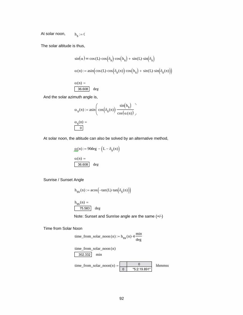
92
At solar noon, hs 0:=
The solar altitude is thus,
sin α( ) cos L( ) cos δs( )⋅ cos hs( )⋅ sin L( ) sin δs( )⋅+
α n( ) asin cos L( ) cos δs n( )( )⋅ cos hs( )⋅ sin L( ) sin δs n( )( )⋅+( ):=
α n( )36.608 deg
=
And the solar azimuth angle is,
αs n( ) asin cos δs n( )( )sin hs( )
cos α n( )( )⋅⎛⎜⎝
⎞⎟⎠
:=
αs n( )0
=
At solar noon, the altitude can also be solved by an alternative method,
α n( ) 90deg L δs n( )−( )−:=
α n( )36.608 deg
=
Sunrise / Sunset Angle
hss n( ) acos tan L( )− tan δs n( )( )⋅( ):=
hss n( )75.583 deg
=
Note: Sunset and Sunrise angle are the same (+/-)
Time from Solar Noon
time_from_solar_noon n( ) hss n( ) 4⋅mindeg
:=
time_from_solar_noon n( )302.332 min
time_from_solar_noon n( ) 0
0 "5:2:19.891"hhmmss=

93
Sunrise will be 12:00 Solar Noon minus the 'time_from_solar_noon(n)' for the given day.
Sunset will be 12:00 Solar Noon plus the 'time_from_solar_noon(n)' for the given day.
Use Equation of Time to convert the Solar Times for sunrise and sunset to local times.
B n( ) 360degn 81−
364⋅:= B n( )
-79.121 deg=
ET n( ) 9.87 sin 2 B n( )⋅( )⋅ 7.53 cos B n( )( )⋅− 1.5 sin B n( )( )⋅−( )min:=
ET n( )-3.607 min
=
1 51 101 151 201 251 301 351
20
10
10
20
Julian Date (1 to 365)
Equa
tion
of T
ime
(min
utes
)
Figure B.2: Equation of Time, in minutes, as a function of the time of year.
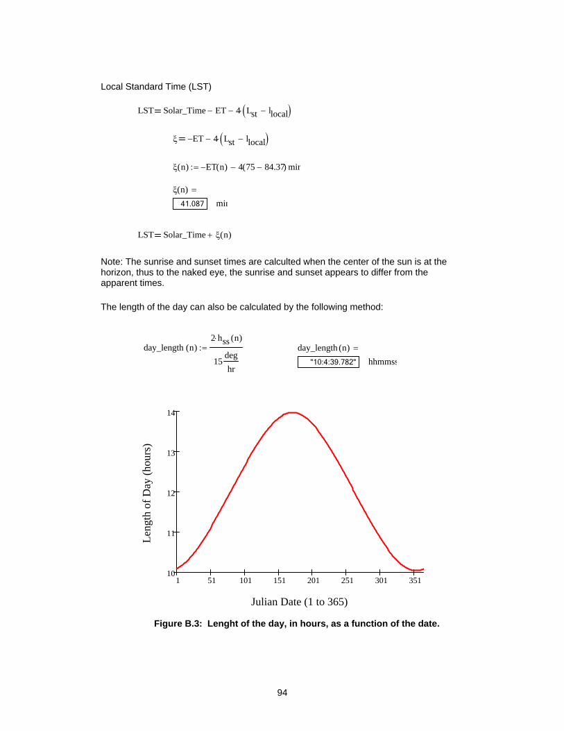
94
Local Standard Time (LST)
LST Solar_Time ET− 4 Lst llocal−( )⋅−
ξ ET− 4 Lst llocal−( )⋅−
ξ n( ) ET n( )− 4 75 84.37−( ) min−:=
ξ n( )41.087 min
=
LST Solar_Time ξ n( )+
Note: The sunrise and sunset times are calculted when the center of the sun is at the horizon, thus to the naked eye, the sunrise and sunset appears to differ from the apparent times.
The length of the day can also be calculated by the following method:
day_length n( )2 hss n( )⋅
15deghr
:= day_length n( )"10:4:39.782" hhmmss
=
1 51 101 151 201 251 301 35110
11
12
13
14
Julian Date (1 to 365)
Leng
th o
f Day
(hou
rs)
Figure B.3: Lenght of the day, in hours, as a function of the date.

95
The instantaneous solar radiation on an object in Tallahassee at 12:00 noon.
The angle of incidence, i, of the beam radiation on a tilted surface, the panel azimuth angle, αw, and the panel tilt angle, β:
Panel tilt angle is same as the solar altitude angle: β n( ) α n( ):=
Panel azimuth angle is same as solar azimuth angle: αw n( ) αs n( ):=
cos i( ) cos α n( )( ) cos αs n( ) αw n( )−( )⋅ sin β n( )( )⋅ sin α n( )( ) cos β n( )( )⋅+
i n( ) acos cos α n( )( ) cos αs n( ) αw n( )−( )⋅ sin β n( )( )⋅ sin α n( )( ) cos β n( )( )⋅+( ):=
i n( )16.783 deg
=
1 51 101 151 201 251 301 351
20
40
60
80
Julian Date (1 to 365)
Ang
le o
f Inc
iden
ce (d
eg)
Figure B.4: Variation of the angle of incidence as a function of the date.
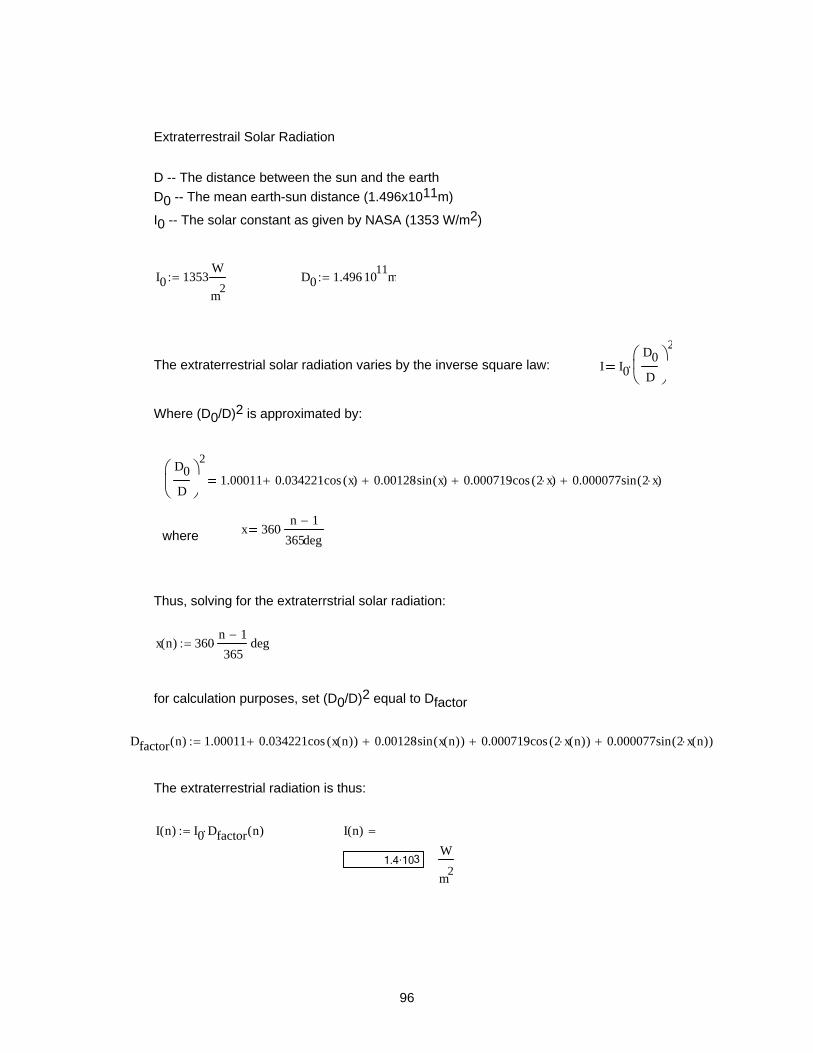
96
Extraterrestrail Solar Radiation
D -- The distance between the sun and the earth D0 -- The mean earth-sun distance (1.496x10¹¹m)
I0 -- The solar constant as given by NASA (1353 W/m2)
I0 1353W
m2:= D0 1.496 1011m⋅:=
The extraterrestrial solar radiation varies by the inverse square law: I I0D0D
⎛⎜⎝
⎞⎟⎠
2
⋅
Where (D0/D)2 is approximated by:
D0D
⎛⎜⎝
⎞⎟⎠
2
1.00011 0.034221cos x( )⋅+ 0.00128sin x( )⋅+ 0.000719cos 2 x⋅( )⋅+ 0.000077sin 2 x⋅( )⋅+
x 360n 1−
365deg⋅ where
Thus, solving for the extraterrstrial solar radiation:
x n( ) 360n 1−
365⋅ deg:=
for calculation purposes, set (D0/D)2 equal to Dfactor
Dfactor n( ) 1.00011 0.034221cos x n( )( )⋅+ 0.00128sin x n( )( )⋅+ 0.000719cos 2 x n( )⋅( )⋅+ 0.000077sin 2 x n( )⋅( )⋅+:=
The extraterrestrial radiation is thus:
I n( ) I0 Dfactor n( )⋅:= I n( )
31.4·10W
m2
=

97
1 51 101 151 201 251 301 3511300
1320
1340
1360
1380
1400
1420
Julian Date (1 to 365)
Extra
terr
estri
al R
adia
tion
(W/m
^2)
Figure B.5: Variation of extraterrestrial solar radiation with time of year.
1 51 101 151 201 251 301 3510.96
0.98
1
1.02
1.04
Julian Date (1 to 365)
Extra
terr
estri
al R
adia
tion/
Sola
r Con
stan
t
Figure B.6: Effect of the time of year of extraterrestraial radiation to the nominal solar constant
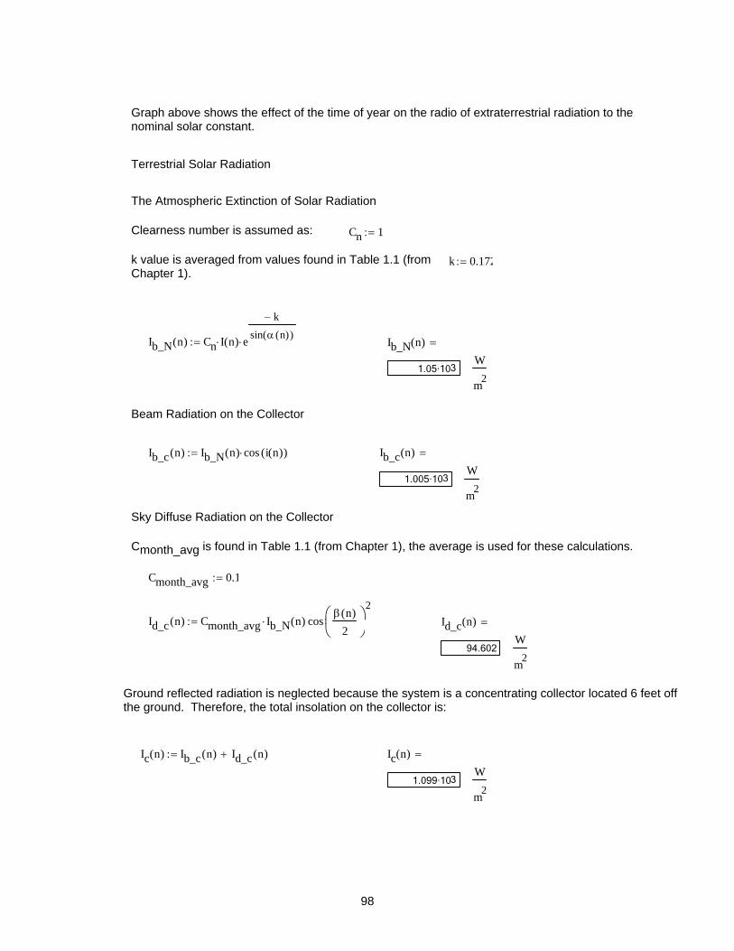
98
Graph above shows the effect of the time of year on the radio of extraterrestrial radiation to the nominal solar constant.
Terrestrial Solar Radiation
The Atmospheric Extinction of Solar Radiation
Clearness number is assumed as: Cn 1:=
k value is averaged from values found in Table 1.1 (from Chapter 1).
k 0.172:=
Ib_N n( ) Cn I n( )⋅ e
k−
sin α n( )( )⋅:= Ib_N n( )
31.05·10W
m2
=
Beam Radiation on the Collector
Ib_c n( ) Ib_N n( ) cos i n( )( )⋅:= Ib_c n( )
31.005·10W
m2
=
Sky Diffuse Radiation on the Collector
Cmonth_avg is found in Table 1.1 (from Chapter 1), the average is used for these calculations.
Cmonth_avg 0.1:=
Id_c n( ) Cmonth_avg Ib_N n( )⋅ cosβ n( )
2⎛⎜⎝
⎞⎟⎠
2:= Id_c n( )
94.602W
m2
=
Ground reflected radiation is neglected because the system is a concentrating collector located 6 feet off the ground. Therefore, the total insolation on the collector is:
Ic n( ) Ib_c n( ) Id_c n( )+:= Ic n( )
31.099·10W
m2
=

99
1 51 101 151 201 251 301 351200
400
600
800
1000
1200
Total InsolationBeam InsolationTotal InsolationBeam Insolation
Julian Date (1 to 365)
Inso
latio
n (W
/m^2
)
Figure B.7: Total Insolation compared to the Beam Insolation incident on the collector.
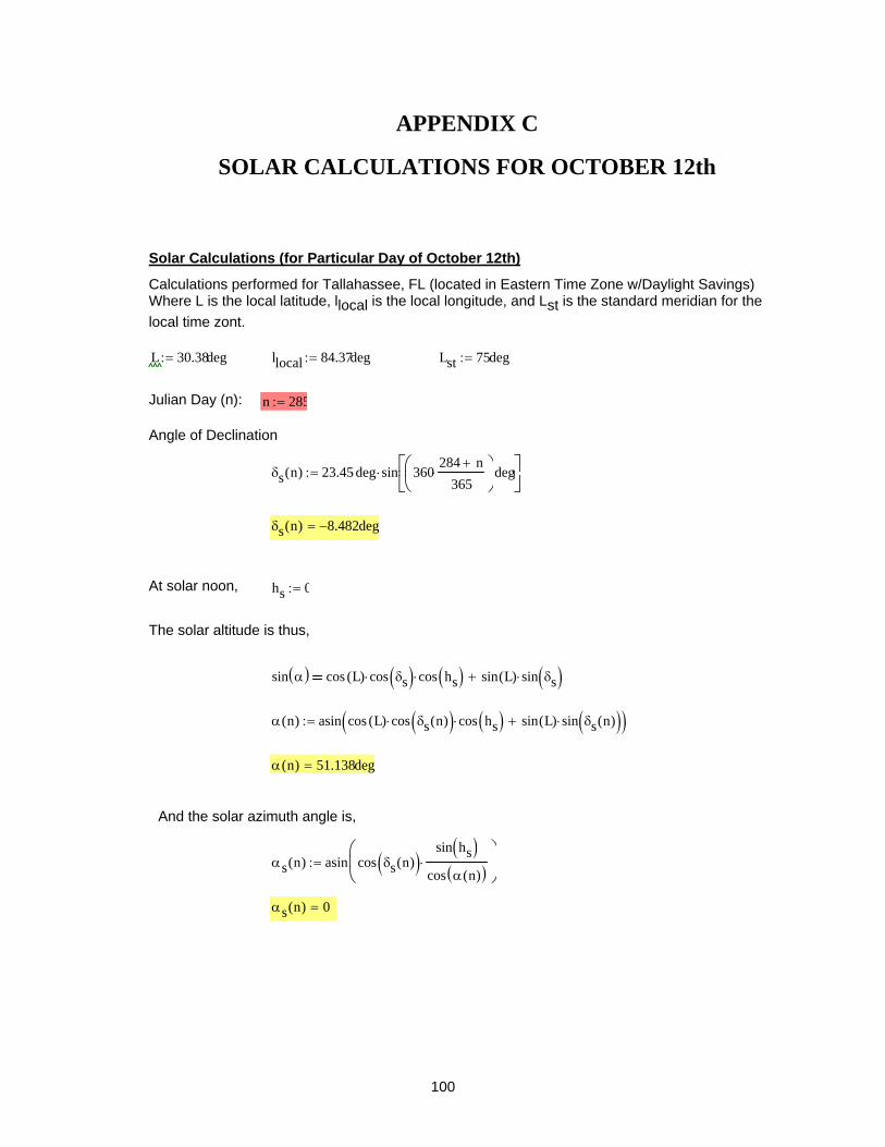
100
APPENDIX C
SOLAR CALCULATIONS FOR OCTOBER 12th
Solar Calculations (for Particular Day of October 12th)
Calculations performed for Tallahassee, FL (located in Eastern Time Zone w/Daylight Savings) Where L is the local latitude, llocal is the local longitude, and Lst is the standard meridian for the local time zont.
L 30.38deg:= llocal 84.37deg:= Lst 75deg:=
Julian Day (n): n 285:=
Angle of Declination
δs n( ) 23.45deg⋅ sin 360284 n+
365⋅⎛⎜
⎝⎞⎟⎠deg⎡⎢
⎣⎤⎥⎦
⋅:=
δs n( ) 8.482− deg=
At solar noon, hs 0:=
The solar altitude is thus,
sin α( ) cos L( ) cos δs( )⋅ cos hs( )⋅ sin L( ) sin δs( )⋅+
α n( ) asin cos L( ) cos δs n( )( )⋅ cos hs( )⋅ sin L( ) sin δs n( )( )⋅+( ):=
α n( ) 51.138deg=
And the solar azimuth angle is,
αs n( ) asin cos δs n( )( )sin hs( )
cos α n( )( )⋅⎛⎜⎝
⎞⎟⎠
:=
αs n( ) 0=

101
Sunrise / Sunset Angle
hss n( ) acos tan L( )− tan δs n( )( )⋅( ):=
hss n( ) 84.984deg=
Note: Sunset and Sunrise angle are the same (+/-)
Time from Solar Noon
time_from_solar_noon n( ) hss n( ) 4⋅mindeg
:=
time_from_solar_noon n( ) 339.938min=
time_from_solar_noon n( ) "5:39:56.27"hhmmss=
Sunrise will be 12:00 Solar Noon minus the 'time_from_solar_noon(n)' for the given day.
Sunset will be 12:00 Solar Noon plus the 'time_from_solar_noon(n)' for the given day.
Use Equation of Time to convert the Solar Times for sunrise and sunset to local times.
B n( ) 360degn 81−
364⋅:= B n( ) 201.758deg=
ET n( ) 9.87 sin 2 B n( )⋅( )⋅ 7.53 cos B n( )( )⋅− 1.5 sin B n( )( )⋅−( )min:=
ET n( ) 14.346min=
Local Standard Time (LST)
LST Solar_Time ET− 4 Lst llocal−( )⋅−
ξ ET− 4 Lst llocal−( )⋅−
ξ n( ) ET n( )− 4 75 84.37−( ) min−:=
ξ n( ) 23.134min=

102
Note: The sunrise and sunset times are calculted when the center of the sun is at the horizon, thus to the naked eye, the sunrise and sunset appears to differ from the apparent times.
The length of the day can also be calculated by the following method:
day_length n( )2 hss n( )⋅
15deghr
:= day_length n( ) "11:19:52.54"hhmmss=
The instantaneous solar radiation on an object in Tallahassee at 12:00 noon.
The angle of incidence, i, of the beam radiation on a tilted surface, the panel azimuth angle, αw, and the panel tilt angle, β:
Panel tilt angle is same as the solar altitude angle: β n( ) α n( ):=
Panel azimuth angle is same as solar azimuth angle: αw n( ) αs n( ):=
cos i( ) cos α n( )( ) cos αs n( ) αw n( )−( )⋅ sin β n( )( )⋅ sin α n( )( ) cos β n( )( )⋅+
i n( ) acos cos α n( )( ) cos αs n( ) αw n( )−( )⋅ sin β n( )( )⋅ sin α n( )( ) cos β n( )( )⋅+( ):=
Angle of Incidence
i n( ) 12.276deg=
Extraterrestrail Solar Radiation
D -- The distance between the sun and the earth D0 -- The mean earth-sun distance (1.496x10¹¹m)
I0 -- The solar constant as given by NASA (1353 W/m2)
I0 1353W
m2:= D0 1.4961011m⋅:=
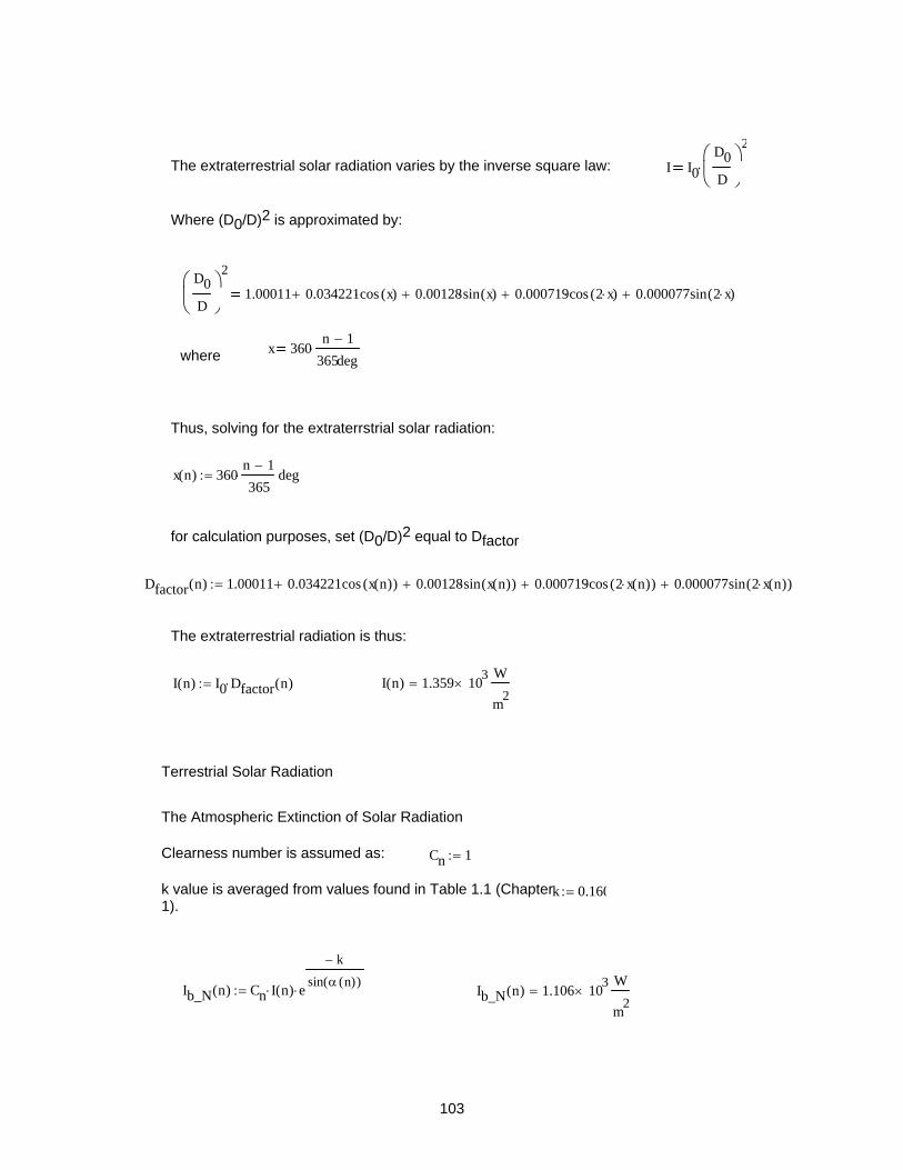
103
The extraterrestrial solar radiation varies by the inverse square law: I I0D0D
⎛⎜⎝
⎞⎟⎠
2
⋅
Where (D0/D)2 is approximated by:
D0D
⎛⎜⎝
⎞⎟⎠
2
1.00011 0.034221cos x( )⋅+ 0.00128sin x( )⋅+ 0.000719cos 2 x⋅( )⋅+ 0.000077sin 2 x⋅( )⋅+
x 360n 1−
365deg⋅ where
Thus, solving for the extraterrstrial solar radiation:
x n( ) 360n 1−
365⋅ deg:=
for calculation purposes, set (D0/D)2 equal to Dfactor
Dfactor n( ) 1.00011 0.034221cos x n( )( )⋅+ 0.00128sin x n( )( )⋅+ 0.000719cos 2 x n( )⋅( )⋅+ 0.000077sin 2 x n( )⋅( )⋅+:=
The extraterrestrial radiation is thus:
I n( ) I0 Dfactor n( )⋅:= I n( ) 1.359 103×
W
m2=
Terrestrial Solar Radiation
The Atmospheric Extinction of Solar Radiation
Clearness number is assumed as: Cn 1:=
k value is averaged from values found in Table 1.1 (Chapter 1).
k 0.160:=
Ib_N n( ) Cn I n( )⋅ e
k−
sin α n( )( )⋅:= Ib_N n( ) 1.106 103
×W
m2=

104
Beam Radiation on the Collector
Ib_c n( ) Ib_N n( ) cos i n( )( )⋅:= Ib_c n( ) 1.081 103×
W
m2=
Sky Diffuse Radiation on the Collector
Cmonth_avg is found in Table 1.1 (Chapter 1), the average is used for these calculations.
Cmonth_avg 0.073:=
Id_c n( ) Cmonth_avg Ib_N n( )⋅ cosβ n( )
2⎛⎜⎝
⎞⎟⎠
2:= Id_c n( ) 65.714
W
m2=
Ground reflected radiation is neglected because the system is a concentrating collector located 6 feet off the ground. Therefore, the total insolation on the collector is:
Ic n( ) Ib_c n( ) Id_c n( )+:= Ic n( ) 1.147 103×
W
m2=
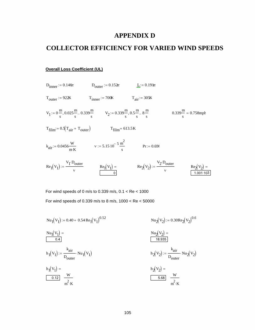
105
APPENDIX D
COLLECTOR EFFICIENCY FOR VARIED WIND SPEEDS
Overall Loss Coefficient (UL)
Dinner 0.146m:= Douter 0.152m:= L 0.191m:=
Touter 922K:= Tinner 700K:= Tair 305K:=
V1 0ms
0.025ms
, 0.339ms
..:= V2 0.339ms
0.5ms
, 8ms
..:= 0.339ms
0.758mph=
Tfilm 0.5 Tair Touter+( ):= Tfilm 613.5K=
kair 0.0456W
m K⋅:= ν 5.15 10 5−
⋅m2
s:= Pr 0.698:=
Re1 V1( )V1 Douter⋅
ν:= Re1 V1( )
0
= Re2 V2( )V2 Douter⋅
ν:= Re2 V2( )
31.001·10
=
For wind speeds of 0 m/s to 0.339 m/s, 0.1 < Re < 1000 For wind speeds of 0.339 m/s to 8 m/s, 1000 < Re < 50000
Nu1 V1( ) 0.40 0.54 Re1 V1( )0.52⋅+:= Nu2 V2( ) 0.30Re2 V2( )0.6
:=
Nu1 V1( )0.4
= Nu2 V2( )18.935
=
h1 V1( )kair
DouterNu1 V1( )⋅:= h2 V2( )
kairDouter
Nu2 V2( )⋅:=
h1 V1( )0.12
W
m2 K⋅
= h2 V2( )5.68
W
m2 K⋅
=
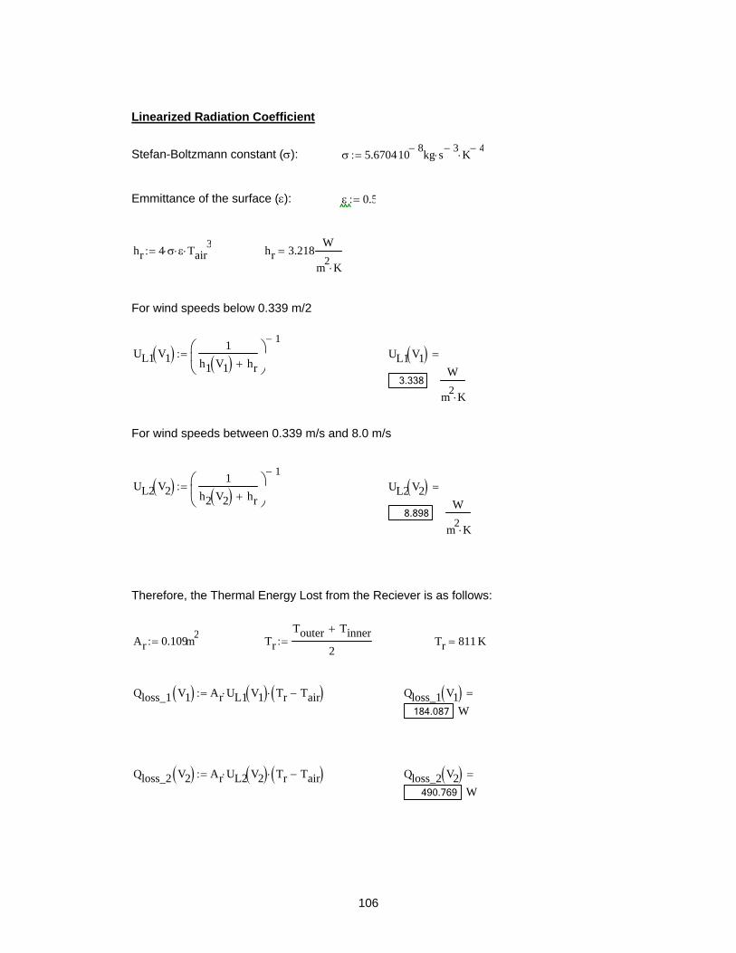
106
Linearized Radiation Coefficient
Stefan-Boltzmann constant (σ): σ 5.670410 8−⋅ kg s 3−
⋅ K 4−⋅:=
Emmittance of the surface (ε): ε 0.5:=
hr 4 σ⋅ ε⋅ Tair3
⋅:= hr 3.218W
m2 K⋅=
For wind speeds below 0.339 m/2
UL1 V1( ) 1h1 V1( ) hr+
⎛⎜⎝
⎞⎟⎠
1−:= UL1 V1( )
3.338W
m2 K⋅
=
For wind speeds between 0.339 m/s and 8.0 m/s
UL2 V2( ) 1h2 V2( ) hr+
⎛⎜⎝
⎞⎟⎠
1−:= UL2 V2( )
8.898W
m2 K⋅
=
Therefore, the Thermal Energy Lost from the Reciever is as follows:
Ar 0.109m2:= Tr
Touter Tinner+
2:= Tr 811 K=
Qloss_1 V1( ) Ar UL1 V1( )⋅ Tr Tair−( )⋅:= Qloss_1 V1( )184.087 W
=
Qloss_2 V2( ) Ar UL2 V2( )⋅ Tr Tair−( )⋅:= Qloss_2 V2( )490.769 W
=

107
0 0.05 0.1 0.15 0.2 0.25 0.3100
200
300
400
500
600
Wind Speed 0 to 0.339 m/s (0 to 0.758 mph)
Hea
t Los
s in
Rec
eive
r (W
atts
)
Figure D.1: Heat loss from receiver for wind speeds less than 0.339 m/s.
2 4 6 80
500
1000
1500
2000
2500
Wind Speed 0.339 to 8 m/s (0.758 to ~18 mph)
Hea
t Los
s in
Rec
eive
r (W
atts
)
Figure D.2: Heat loss from receiver for wind speeds greater than 0.339 m/s.

108
Optical Energy Absorbed by the Receiver
Qopt Aa ρ s_m⋅ τg⋅ αr⋅ R⋅ S⋅ Ia⋅
ρs_m -- specular reflectance of concentrating mirror τg -- transmittance of any glass envelope covering the receiver Aa -- aperture area of the collector S -- receiver shading factor (fraction of collector aperture not shadowed by the recevier) Ia -- insolation incident on the collector aperture αr -- absorbtance of the receiver
S, αr, ρs_m, and τg are constants dependent only on the materials used and the structure accuracy of the collector. These constants are nominally lumped into a single constant term, ηopt, the optical efficiency of the collector.
S 1:= αr 0.99:= ρ s_m 1:= τg 1:= Aa 10.507m2:=
Ia 1064W
m2:= k 103
:=
Qopt Aa ρ s_m⋅ τg⋅ αr⋅ S⋅ Ia⋅:= Qopt 11.068k W⋅=
Thus, the quantity of thermal energy produced by the solar collector is described by:
Qout_1 V1( ) Qopt Qloss_1 V1( )−:= Qout_1 V1( )41.088·10 W=
Qout_2 V2( ) Qopt Qloss_2 V2( )−:= Qout_2 V2( )41.058·10 W=
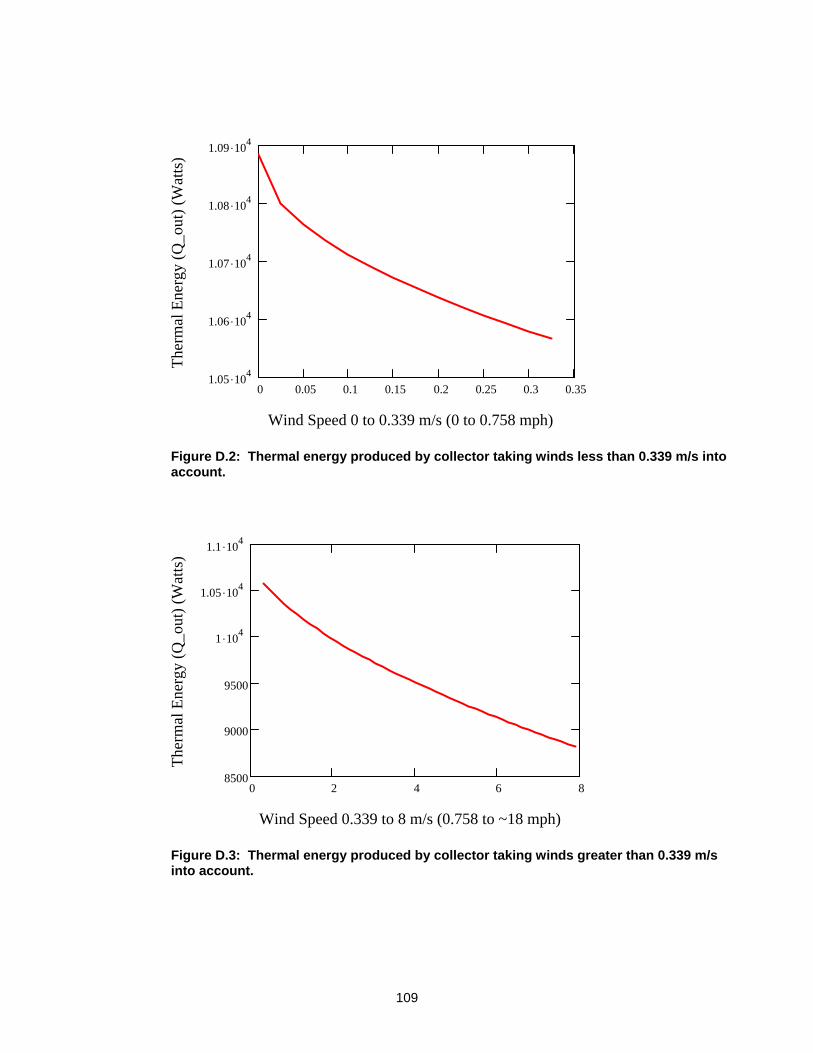
109
0 0.05 0.1 0.15 0.2 0.25 0.3 0.351.05 .104
1.06 .104
1.07 .104
1.08 .104
1.09 .104
Wind Speed 0 to 0.339 m/s (0 to 0.758 mph)
Ther
mal
Ene
rgy
(Q_o
ut) (
Wat
ts)
Figure D.2: Thermal energy produced by collector taking winds less than 0.339 m/s into account.
0 2 4 6 88500
9000
9500
1 .104
1.05 .104
1.1 .104
Wind Speed 0.339 to 8 m/s (0.758 to ~18 mph)
Ther
mal
Ene
rgy
(Q_o
ut) (
Wat
ts)
Figure D.3: Thermal energy produced by collector taking winds greater than 0.339 m/s into account.

110
Collector Efficiency
ηcollector_1 V1( )Qout_1 V1( )
Aa Ia⋅:= ηcollector_1 V1( )
97.353 %
0 0.05 0.1 0.15 0.2 0.25 0.3 0.350.94
0.95
0.96
0.97
0.98
Wind Speed 0 to 0.339 m/s (0 to 0.758 mph)
Col
lect
or E
ffic
ienc
y
Figure D.4: Effects of collector efficiency for wind speeds less than 0.339 m/s.
ηcollector_2 V2( )Qout_2 V2( )
Aa Ia⋅:= ηcollector_2 V2( )
94.61 %
0 2 4 6 80.75
0.8
0.85
0.9
0.95
Wind Speed 0.339 to 8 m/s (0.758 to ~18 mph)
Col
lect
or E
ffic
ienc
y
Figure D.5: Effects of collector efficiency for wind speeds greater than 0.339 m/s.
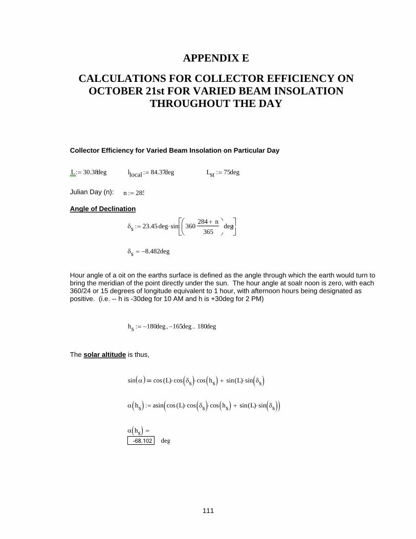
111
APPENDIX E
CALCULATIONS FOR COLLECTOR EFFICIENCY ON OCTOBER 21st FOR VARIED BEAM INSOLATION
THROUGHOUT THE DAY
Collector Efficiency for Varied Beam Insolation on Particular Day
L 30.38deg:= llocal 84.37deg:= Lst 75deg:=
Julian Day (n): n 285:=
Angle of Declination
δs 23.45 deg⋅ sin 360284 n+
365⋅⎛⎜
⎝⎞⎟⎠
deg⎡⎢⎣
⎤⎥⎦
⋅:=
δs 8.482− deg=
Hour angle of a oit on the earths surface is defined as the angle through which the earth would turn to bring the meridian of the point directly under the sun. The hour angle at soalr noon is zero, with each 360/24 or 15 degrees of longitude equivalent to 1 hour, with afternoon hours being designated as positive. (i.e. -- h is -30deg for 10 AM and h is +30deg for 2 PM)
hs 180− deg 165− deg, 180deg..:=
The solar altitude is thus,
sin α( ) cos L( ) cos δs( )⋅ cos hs( )⋅ sin L( ) sin δs( )⋅+
α hs( ) asin cos L( ) cos δs( )⋅ cos hs( )⋅ sin L( ) sin δs( )⋅+( ):=
α hs( )-68.102 deg
=
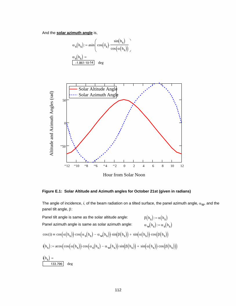
112
And the solar azimuth angle is,
αs hs( ) asin cos δs( )sin hs( )
cos α hs( )( )⋅
⎛⎜⎝
⎞⎟⎠
:=
αs hs( )-14-1.861·10 deg
=
12 10 8 6 4 2 0 2 4 6 8 10 12
50
0
50
Solar Altitude AngleSolar Azimuth AngleSolar Altitude AngleSolar Azimuth Angle
Hour from Solar Noon
Alti
tude
and
Azi
mut
h A
ngle
s (ra
d)
Figure E.1: Solar Altitude and Azimuth angles for October 21st (given in radians)
The angle of incidence, i, of the beam radiation on a tilted surface, the panel azimuth angle, αw, and the panel tilt angle, β:
Panel tilt angle is same as the solar altitude angle: β hs( ) α hs( ):=
Panel azimuth angle is same as solar azimuth angle: αw hs( ) αs hs( ):=
cos i( ) cos α hs( )( ) cos αs hs( ) αw hs( )−( )⋅ sin β hs( )( )⋅ sin α hs( )( ) cos β hs( )( )⋅+
i hs( ) acos cos α hs( )( ) cos αs hs( ) αw hs( )−( )⋅ sin β hs( )( )⋅ sin α hs( )( ) cos β hs( )( )⋅+( ):=
i hs( )133.796 deg=

113
15 10 5 0 5 10 15
50
100
150
200
Hour From Solar Noon
Ang
le o
f Inc
iden
ce (d
eg)
Figure E.2: Angle of incidence on October 21st for time from solar noon.
Extraterrestrail Solar Radiation
D -- The distance between the sun and the earth D0 -- The mean earth-sun distance (1.496x10¹¹m)
I0 -- The solar constant as given by NASA (1353 W/m2)
I0 1353W
m2:= D0 1.496 1011m⋅:=
The extraterrestrial solar radiation varies by the inverse square law: I I0D0D
⎛⎜⎝
⎞⎟⎠
2
⋅
Where (D0/D)2 is approximated by:
D0D
⎛⎜⎝
⎞⎟⎠
2
1.00011 0.034221cos x( )⋅+ 0.00128sin x( )⋅+ 0.000719cos 2 x⋅( )⋅+ 0.000077sin 2 x⋅( )⋅+
x 360n 1−
365deg⋅ where

114
Thus, solving for the extraterrstrial solar radiation:
x 360n 1−
365⋅ deg:=
for calculation purposes, set (D0/D)2 equal to Dfactor
Dfactor 1.00011 0.034221cos x( )⋅+ 0.00128sin x( )⋅+ 0.000719cos 2 x⋅( )⋅+ 0.000077sin 2 x⋅( )⋅+:=
The extraterrestrial radiation is thus:
I I0 Dfactor⋅:= I 1.359 103×
W
m2=
Terrestrial Solar Radiation
The Atmospheric Extinction of Solar Radiation
Clearness number is assumed as: Cn 1:=
k value is averaged from values found in Table ##. k 0.172:=
Ib_N hs( ) Cn I⋅ e
k−
sin α hs( )( )⋅:= Ib_N hs( )
31.635·10W
m2
=
Beam Radiation on the Collector
Ib_c hs( ) Ib_N hs( ) cos i hs( )( )⋅:= Ib_c hs( )3-1.132·10
W
m2
=
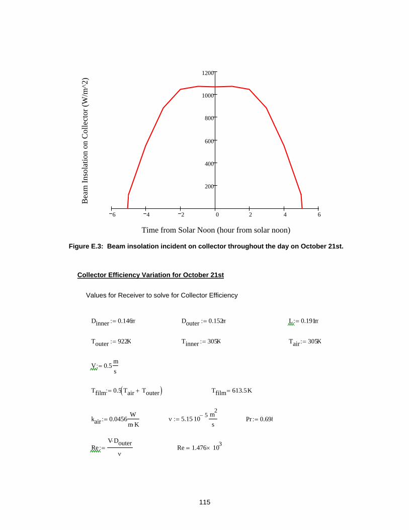
115
6 4 2 0 2 4 6
200
400
600
800
1000
1200
Time from Solar Noon (hour from solar noon)
Bea
m In
sola
tion
on C
olle
ctor
(W/m
^2)
Figure E.3: Beam insolation incident on collector throughout the day on October 21st.
Collector Efficiency Variation for October 21st
Values for Receiver to solve for Collector Efficiency
Dinner 0.146m:= Douter 0.152m:= L 0.191m:=
Touter 922K:= Tinner 305K:= Tair 305K:=
V 0.5ms
:=
Tfilm 0.5 Tair Touter+( ):= Tfilm 613.5K=
kair 0.0456W
m K⋅:= ν 5.15 10 5−
⋅m2
s:= Pr 0.698:=
ReV Douter⋅
ν:= Re 1.476 103
×=
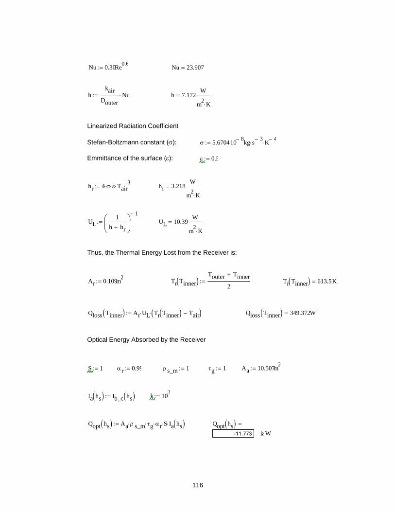
116
Nu 0.30Re0.6:= Nu 23.907=
hkair
DouterNu⋅:= h 7.172
W
m2 K⋅=
Linearized Radiation Coefficient
Stefan-Boltzmann constant (σ): σ 5.670410 8−⋅ kg s 3−
⋅ K 4−⋅:=
Emmittance of the surface (ε): ε 0.5:=
hr 4 σ⋅ ε⋅ Tair3
⋅:= hr 3.218W
m2 K⋅=
UL1
h hr+⎛⎜⎝
⎞⎟⎠
1−:= UL 10.39
W
m2 K⋅=
Thus, the Thermal Energy Lost from the Receiver is:
Ar 0.109m2:= Tr Tinner( )
Touter Tinner+
2:= Tr Tinner( ) 613.5K=
Qloss Tinner( ) Ar UL⋅ Tr Tinner( ) Tair−( )⋅:= Qloss Tinner( ) 349.372W=
Optical Energy Absorbed by the Receiver
S 1:= αr 0.99:= ρ s_m 1:= τg 1:= Aa 10.507m2:=
Ia hs( ) Ib_c hs( ):= k 103:=
Qopt hs( ) Aa ρ s_m⋅ τg⋅ αr⋅ S⋅ Ia hs( )⋅:= Qopt hs( )-11.773 k W⋅
=

117
Thus, the quantity of thermal energy produced by the solar collector is described by:
Qout hs Tinner,( ) Qopt hs( ) Qloss Tinner( )−:= Qout hs Tinner,( )4-1.212·10 W
Collector Efficiency
ηcollector hs Tinner,( )Qout hs Tinner,( )
Aa Ia hs( )⋅:= ηcollector hs Tinner,( )
101.938 %
HT hs Tinner,( )Tinner Tair−
Ia hs( ):= HT hs Tinner,( )
0m2 K⋅
W
=
6 4 2 0 2 4 60.7
0.8
0.9
Overall Collector EfficiencySolar Noon1 PM2 PM3 PM4 PM5 PM6 PM
Overall Collector EfficiencySolar Noon1 PM2 PM3 PM4 PM5 PM6 PM
Hour Angle (Hours from Solar Noon)
Col
lect
or E
ffic
ienc
y
Figure E.4: Collector efficiency due to beam insolation variation for October 21st.
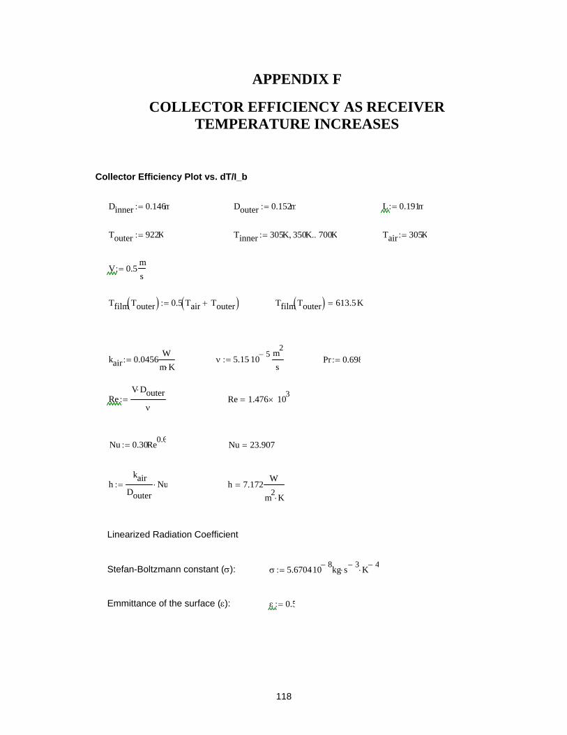
118
APPENDIX F
COLLECTOR EFFICIENCY AS RECEIVER TEMPERATURE INCREASES
Collector Efficiency Plot vs. dT/I_b
Dinner 0.146m:= Douter 0.152m:= L 0.191m:=
Touter 922K:= Tinner 305K 350K, 700K..:= Tair 305K:=
V 0.5ms
:=
Tfilm Touter( ) 0.5 Tair Touter+( ):= Tfilm Touter( ) 613.5K=
kair 0.0456W
m K⋅:= ν 5.15 10 5−
⋅m2
s:= Pr 0.698:=
ReV Douter⋅
ν:= Re 1.476 103
×=
Nu 0.30Re0.6:= Nu 23.907=
hkair
DouterNu⋅:= h 7.172
W
m2 K⋅=
Linearized Radiation Coefficient
Stefan-Boltzmann constant (σ): σ 5.670410 8−⋅ kg s 3−
⋅ K 4−⋅:=
Emmittance of the surface (ε): ε 0.5:=
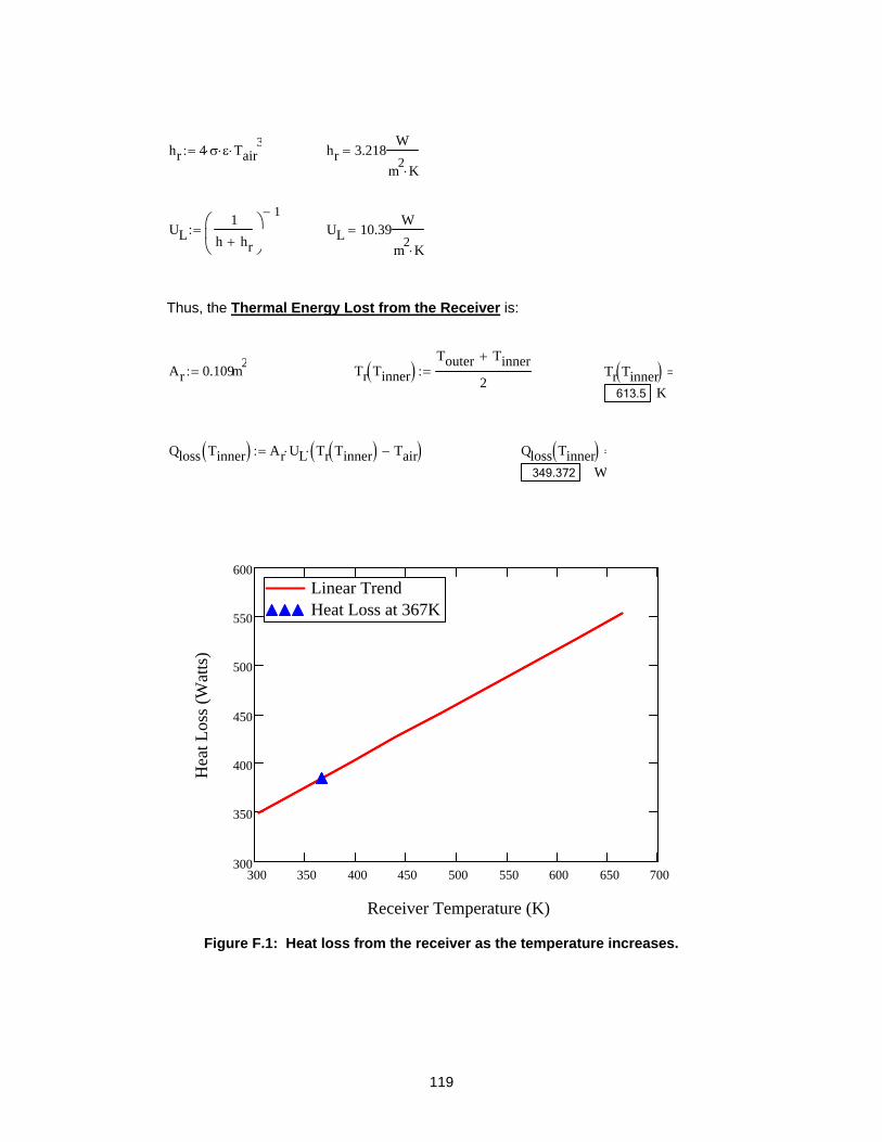
119
hr 4 σ⋅ ε⋅ Tair3
⋅:= hr 3.218W
m2 K⋅=
UL1
h hr+⎛⎜⎝
⎞⎟⎠
1−:= UL 10.39
W
m2 K⋅=
Thus, the Thermal Energy Lost from the Receiver is:
Ar 0.109m2:= Tr Tinner( )
Touter Tinner+
2:= Tr Tinner( )
613.5 K=
Qloss Tinner( ) Ar UL⋅ Tr Tinner( ) Tair−( )⋅:= Qloss Tinner( )349.372 W
=
300 350 400 450 500 550 600 650 700300
350
400
450
500
550
600Linear TrendHeat Loss at 367KLinear TrendHeat Loss at 367K
Receiver Temperature (K)
Hea
t Los
s (W
atts
)
Figure F.1: Heat loss from the receiver as the temperature increases.
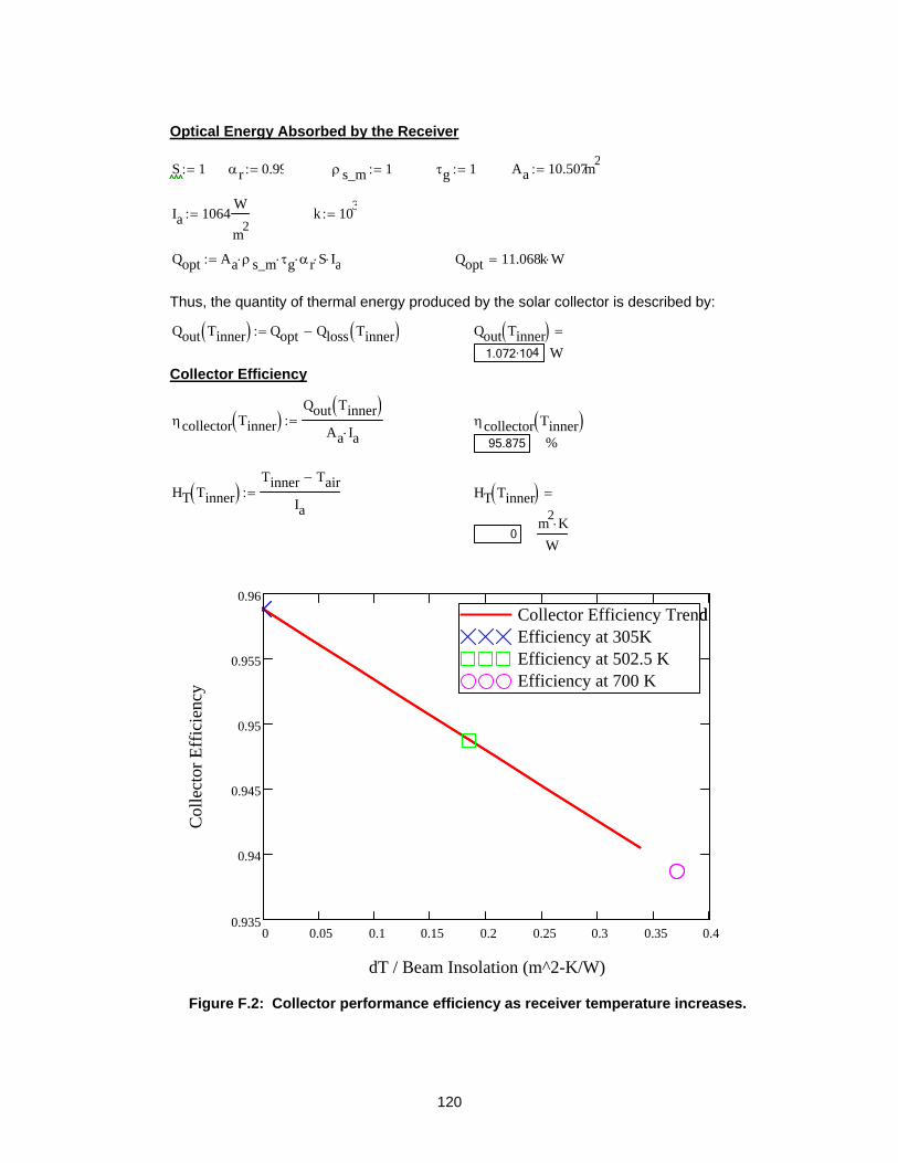
120
Optical Energy Absorbed by the Receiver
S 1:= αr 0.99:= ρ s_m 1:= τg 1:= Aa 10.507m2:=
Ia 1064W
m2:= k 103
:=
Qopt Aa ρ s_m⋅ τg⋅ αr⋅ S⋅ Ia⋅:= Qopt 11.068k W⋅=
Thus, the quantity of thermal energy produced by the solar collector is described by:
Qout Tinner( ) Qopt Qloss Tinner( )−:= Qout Tinner( )41.072·10 W
=
Collector Efficiency
ηcollector Tinner( )Qout Tinner( )
Aa Ia⋅:= ηcollector Tinner( )
95.875 %
HT Tinner( )Tinner Tair−
Ia:= HT Tinner( )
0m2 K⋅
W
=
0 0.05 0.1 0.15 0.2 0.25 0.3 0.35 0.40.935
0.94
0.945
0.95
0.955
0.96Collector Efficiency TrendEfficiency at 305KEfficiency at 502.5 KEfficiency at 700 K
Collector Efficiency TrendEfficiency at 305KEfficiency at 502.5 KEfficiency at 700 K
dT / Beam Insolation (m^2-K/W)
Col
lect
or E
ffic
ienc
y
Figure F.2: Collector performance efficiency as receiver temperature increases.

121
APPENDIX G
GEOMETRIC CONCENTRATION RATIO
AND
MAXIMUM THEORETICAL TEMPERATURE
Operating Temperature as a Function of Concentration
Assume the sun and the rest of the universe to be blackbodies. The sun is at a surface temperature of Tsun; the rest of the universe (other than the sun and the receiver/absorber) is at Tamb, which is equal to zero.
Tsun 6000K:= Tsun 5726.85°C= k 103:=
Tamb 0K:=
Radius of the sun (r): rsun 695500km:=
Stefan-Boltzmann constant (σ): σ 5.670410 8−⋅ kg s 3−
⋅ K 4−⋅:=
Radiation emitted by the sun:
Qsun 4 π⋅ rsun2
⋅ σ⋅ Tsun4
⋅:= Qsun 4.467 1023× kW=
Radiation incident on a collector of aperture area (Aconcentrator):
Dimensions of the Concentrator H: Depth D: Diameter
D 12ft:= H 25.5in:=
PD2
8 H⋅:= P 2.582m=
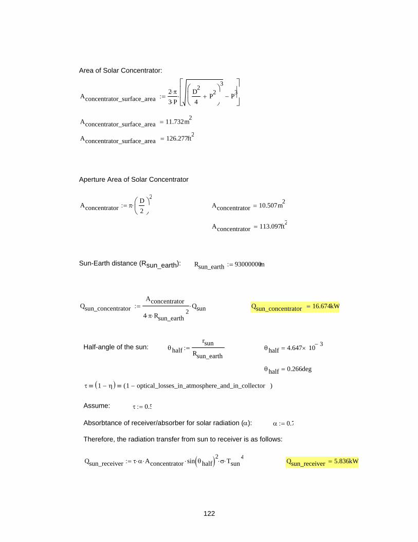
122
Area of Solar Concentrator:
Aconcentrator_surface_area2 π⋅
3 P⋅D2
4P2
+⎛⎜⎝
⎞⎟⎠
3
P3−
⎡⎢⎢⎣
⎤⎥⎥⎦
⋅:=
Aconcentrator_surface_area 11.732m2=
Aconcentrator_surface_area 126.277ft2=
Aperture Area of Solar Concentrator
Aconcentrator πD2
⎛⎜⎝
⎞⎟⎠
2⋅:= Aconcentrator 10.507m2
=
Aconcentrator 113.097ft2=
Sun-Earth distance (Rsun_earth): Rsun_earth 93000000mi:=
Qsun_concentratorAconcentrator
4 π⋅ Rsun_earth2
⋅Qsun⋅:= Qsun_concentrator 16.674kW=
Half-angle of the sun: θhalfrsun
Rsun_earth:= θhalf 4.647 10 3−
×=
θhalf 0.266deg=
τ 1 η−( ) 1 optical_losses_in_atmosphere_and_in_collector−( )
Assume: τ 0.5:=
Absorbtance of receiver/absorber for solar radiation (α): α 0.7:=
Therefore, the radiation transfer from sun to receiver is as follows:
Qsun_receiver τ α⋅ Aconcentrator⋅ sin θhalf( )2⋅ σ⋅ Tsun4
⋅:= Qsun_receiver 5.836kW=

123
Emittance of the absorber in infrared region (ε): ε 0.5:=
Dimensions of Receiver h: Height d: Diameter
h 7.5in:= d 6in:=
Abase πd2
⎛⎜⎝
⎞⎟⎠
2⋅:= Abase 0.018m2
=
Asides d π⋅ h⋅:= Asides 0.091m2=
Areceiver Abase Asides+:= Areceiver 0.109m2=
The radiation losses from the receiver are thus:
Qreceiver_radiation ε Areceiver⋅ σ⋅ Treceiver⋅
A fraction (η) of the incoming solar radiation Qsun_receiver is used in the useful heat transfer to the working fluid and/or is lost by convection/conduction. Thus, the energy balance equation for the receiver is:
Qsun_receiver Qreceiver_radiation η Qsun_receiver⋅+
This equation can also be presented as:
1 η−( ) τ⋅ α⋅ Aconcentrator⋅ sin θhalf( )2⋅ Tsun4
⋅ ε Areceiver⋅ Treceiver4
⋅
Assume that: η 0.5:=
Geometric Concentration Ratio
CRgeometricAconcentrator
Areceiver:= CRgeometric 96=

124
Ideal Concentration Ratio
CRideal1
sin θhalf( )2:= CRideal 4.631 104
×=
The operating temperature of the receiver can now be found:
Treceiver Tsun 1 η−( ) τ⋅ α
ε⋅
CRgeometricCRideal
⋅⎡⎢⎣
⎤⎥⎦
1
4
⋅:= Treceiver 984.732K=
Treceiver 711.582°C=
Treceiver 1.313 103× °F=
Note: As Treceiver approaches Tsun, the highest possible absorber temperature, Treceiver_max, is equal to Tsun, which is approximately 6000K. This temperature is only in theory and could only ever be achieved if no heat is extracted and the concentration ration was equal to 45300.

125
APPENDIX H
GEOMETRIC CONCENTRATION RATIO AS FUNTION OF RECEIVER TEMPERATURE
Concentration Ration as a Function of Receiver Temperature
Tsun 6000K:= Tsun 5726.85°C=
Tamb 0K:=
Radius of the sun (r): rsun 695500km:=
Stefan-Boltzmann constant (σ): σ 5.670410 8−⋅ kg s 3−
⋅ K 4−⋅:=
Radiation emitted by the sun:
Qsun 4 π⋅ rsun2
⋅ σ⋅ Tsun4
⋅:= Qsun 4.467 1023× kW=
Radiation incident on a collector of aperture area (Aconcentrator):
Dimensions of the Concentrator H: Depth D: Diameter
D 12ft:= H 25.5in:=
Aperture Area of Solar Concentrator:
Aconcentrator πD2
⎛⎜⎝
⎞⎟⎠
2⋅:= Aconcentrator 10.507m2
=
Aconcentrator 113.097ft2=
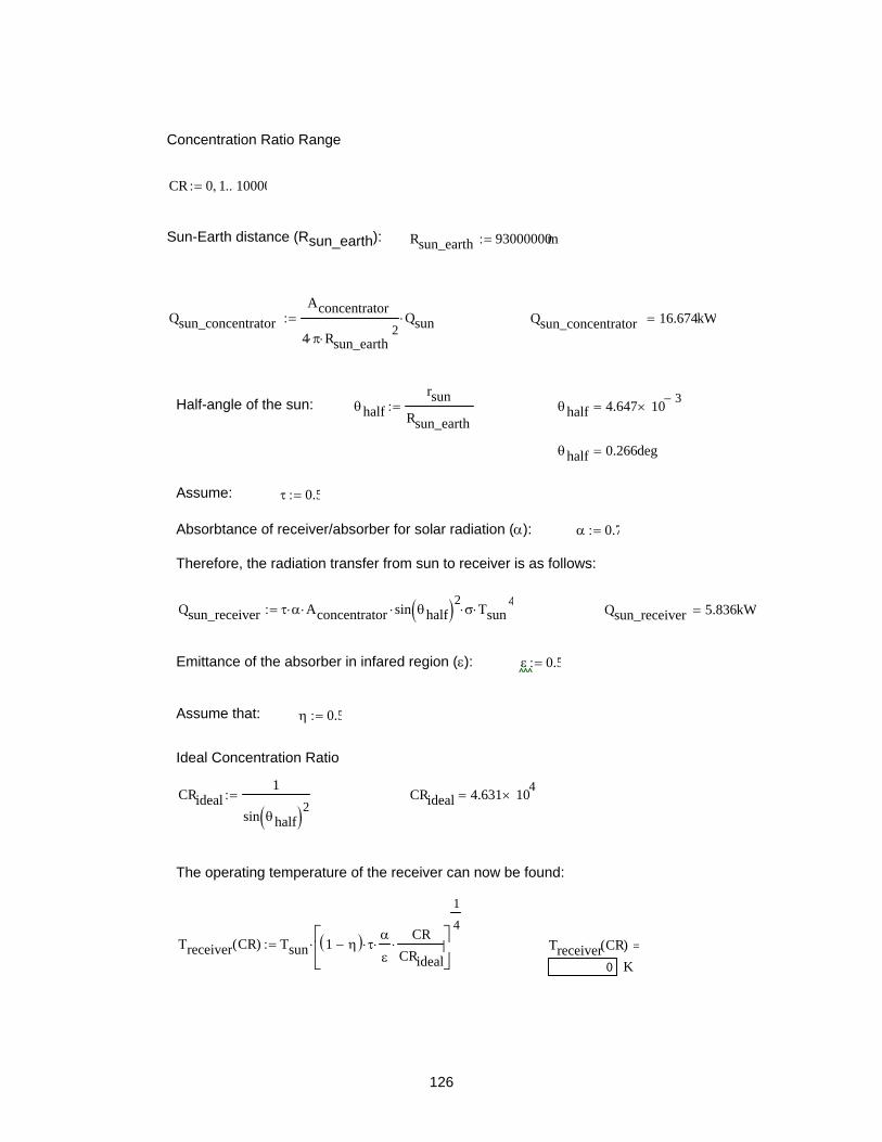
126
Concentration Ratio Range
CR 0 1, 10000..:=
Sun-Earth distance (Rsun_earth): Rsun_earth 93000000mi:=
Qsun_concentratorAconcentrator
4 π⋅ Rsun_earth2
⋅Qsun⋅:= Qsun_concentrator 16.674kW=
Half-angle of the sun: θhalfrsun
Rsun_earth:= θhalf 4.647 10 3−
×=
θhalf 0.266deg=
Assume: τ 0.5:=
Absorbtance of receiver/absorber for solar radiation (α): α 0.7:=
Therefore, the radiation transfer from sun to receiver is as follows:
Qsun_receiver τ α⋅ Aconcentrator⋅ sin θhalf( )2⋅ σ⋅ Tsun4
⋅:= Qsun_receiver 5.836kW=
Emittance of the absorber in infared region (ε): ε 0.5:=
Assume that: η 0.5:=
Ideal Concentration Ratio
CRideal1
sin θhalf( )2:= CRideal 4.631 104
×=
The operating temperature of the receiver can now be found:
Treceiver CR( ) Tsun 1 η−( ) τ⋅ α
ε⋅
CRCRideal⋅⎡
⎢⎣
⎤⎥⎦
1
4⋅:= Treceiver CR( )
0 K=

127
0 500 1000 1500 2000 2500 3000 35001
10
100
1 .103
1 .104
CR vs TemperatureActualIdeal
CR vs TemperatureActualIdeal
Receiver Temperature (K)
Con
cent
ratio
n R
atio
Figure H.1: Concentration given as a function of the operating temperature. For our system, the ideal concentration ratio of 96 is given at the point which falls on the curve. In reality, our system falls slightly behind the curve.

128
APPENDIX I
RECEIVER / BOILER EFFICIENCY CALCULATIONS
Boiler Efficiency k 103:=
Direct Method
Directly defined by the exploitable heat output from the boiler and bythe fuel power input of the boiler.
ηboiler_directQoutputQinput
Indirect Method
Determines efficiency by the sum of the major losses and by the fuel power of the boiler. The indirect method provides a better understanding of the individual losses on the boiler efficiency.
ηboiler_indirect 1QlossesQinput
−
Qlosses 349.372W:= Qinput 11.072k W⋅:= Qoutput 1k W⋅:=
ηboiler_directQoutputQinput
:= ηboiler_direct 9.032%=
ηboiler_indirect 1QlossesQinput
−:= ηboiler_indirect 96.845%=

129
APPENDIX J
MASS FLOW RATE CALCULATIONS
FOR STEAM INTO TURBINE
Mass Flow Rate through Steam Turbine Nozzle
Area of the Steam Turbine Nozzle
d 0.09in:= A πd2
⎛⎜⎝
⎞⎟⎠
2⋅:= A 4.104 10 6−
× m2=
Speed of Sound Properties for Steam
Tsteam 373.15K:= R 461.4N m⋅kg K⋅
:= ρ 0.60kg
m3:= γ 1.324:=
Turbine Inlet Steam Temperature Turbine Inlet Steam Pressure k 103:=
T 470K:= Pt 0.480537MPa:=
From the Steam Tables for the given pressure and temperature
ts 448.51K:= ν 0.4394m3
kg:= s 7.0648
k J⋅kg K⋅
:=
Since the inlet temperature is higher than the saturation temperature, the steam is superheated.
Speed of Sound
aγ Pt⋅
ρ:= a 1.03 103
×ms
=
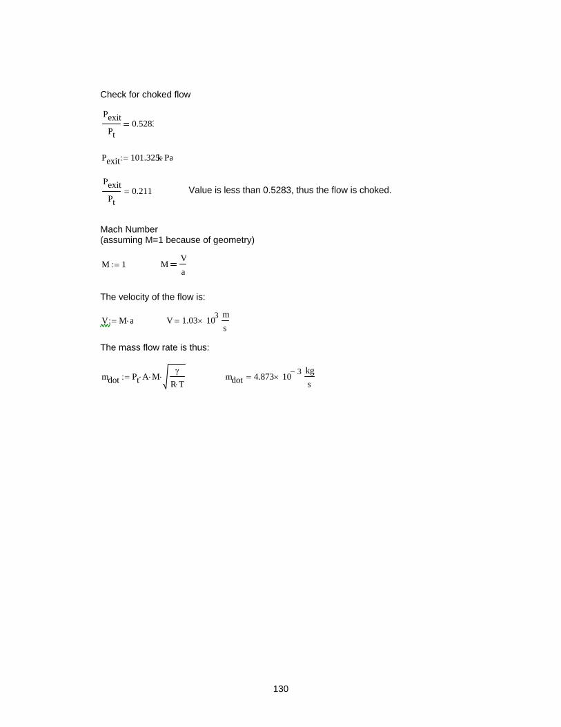
130
Check for choked flow
PexitPt
0.5283
Pexit 101.325k Pa⋅:=
PexitPt
0.211= Value is less than 0.5283, thus the flow is choked.
Mach Number (assuming M=1 because of geometry)
M 1:= MVa
The velocity of the flow is:
V M a⋅:= V 1.03 103×
ms
=
The mass flow rate is thus:
mdot Pt A⋅ M⋅γ
R T⋅⋅:= mdot 4.873 10 3−
×kgs
=

131
APPENDIX K
STEAM TURBINE EFFICIENCY CALCULATIONS
Steam Turbine Calculations
k 103:=
Mass Flow Rate into the turbine: mdot 4.87310 3−⋅
kgs
:=
Enthalpy Values for Turbine Inlet (h3) and Outlet (h4): h3 2764.0848k J⋅kg
:= h4 2679.7689k J⋅kg
:=
Heat Transfer from the Turbine: Qdot mdot h4 h3−( )⋅:=
Qdot 410.871− W=
Pinlet 480.537k Pa⋅:= Poutlet 101.325k Pa⋅:=
Tinlet 431.46K:=
mdot ρ in Vinlet⋅ Anozzle⋅ mdot ρout Vout⋅ Anozzle⋅
Anozzle 4.10410 6−⋅ m2
:= Aexit 1.26710 4−⋅ m2
:= ρ in 2.2760kg
m3:= ρout 0.5409
kg
m3:=
Vinletmdot
ρ in Anozzle⋅:= Voutlet
mdotρout Aexit⋅
:=
Vinlet 521.695ms
= Voutlet 71.105ms
=

132
Elevation of turbine inlet and outlet above reference plane:
Zinlet 10in:= Zoutlet 6in:=
From the Steam Tables:
hinlet h3:= houtlet h4:=
Qdot mdot hinletVinlet
2
2+ g Zinlet⋅+
⎛⎜⎜⎝
⎞⎟⎟⎠
⋅+ mdot houtletVoutlet
2
2+ g Zoutlet⋅+
⎛⎜⎜⎝
⎞⎟⎟⎠
⋅ Wdot_CV+
Wdot_CV Qdot mdot hinletVinlet
2
2+ g Zinlet⋅+
⎛⎜⎜⎝
⎞⎟⎟⎠
⋅+ mdot houtletVoutlet
2
2+ g Zoutlet⋅+
⎛⎜⎜⎝
⎞⎟⎟⎠
⋅−:=
Wdot_CV 650.818W= Power Output of the Turbine
Work Output of the Turbine is solved by:
waWdot_CV
mdot:= wa 133.556
k J⋅kg
=
To determine the efficiency of the turbine (or any machine in that matter), we compare the actual performacne of the machine under given conditions to the performance that would have been achieved in an ideal process. A steam turbine is inteded to be an adiabatic machine. The only heat transfer which takes place is the unavoidable heat transfer between the turbine and its surroundings. Also, we consider the turbine to be running at steady-state, steady-flow, thus, the state of the steam entering the turbine and the exhaust pressure are fixed. Thsu, the ideal process is considered to be a reversible adiabatic process (which is also an isentropic process), between the turbine inlet state and the turbine exhaust pressure. Thus, if we denote the actual work done per unit mass of steam flow thorugh the turbine as wa and the work that would be done in an ideal cycle as ws, the efficiency fo the turbine is thus defined as:
η turbinewaws
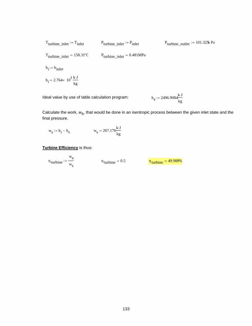
133
Tturbine_inlet Tinlet:= Pturbine_inlet Pinlet:= Pturbine_outlet 101.325k Pa⋅:=
Tturbine_inlet 158.31°C= Pturbine_inlet 0.481MPa=
hi hinlet:=
hi 2.764 103×
k J⋅kg
=
Ideal value by use of table calculation program: he 2496.9084k J⋅kg
:=
Calculate the work, ws, that would be done in an isentropic process between the given inlet state and the final pressure.
ws hi he−:= ws 267.176k J⋅kg
=
Turbine Efficiency is thus:
η turbinewaws
:= η turbine 0.5= η turbine 49.988%=
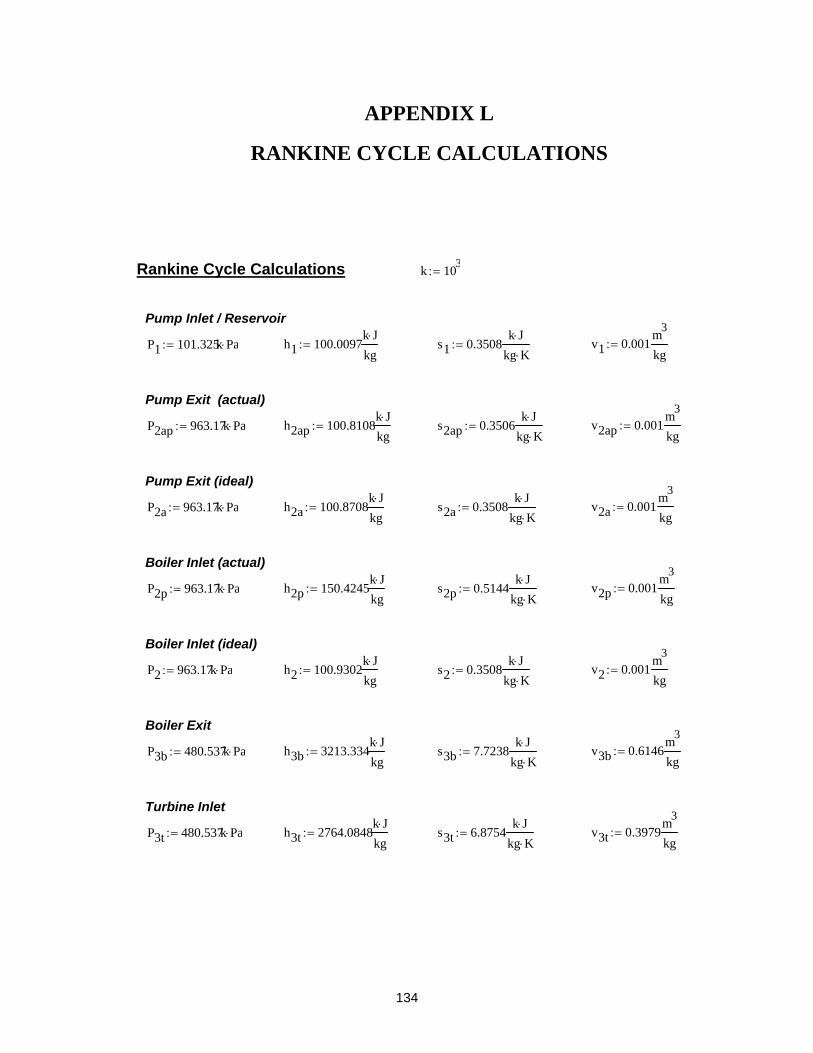
134
APPENDIX L
RANKINE CYCLE CALCULATIONS
Rankine Cycle Calculations k 103:=
Pump Inlet / Reservoir
P1 101.325k Pa⋅:= h1 100.0097k J⋅kg
:= s1 0.3508k J⋅
kg K⋅:= v1 0.001
m3
kg:=
Pump Exit (actual)
P2ap 963.17k Pa⋅:= h2ap 100.8108k J⋅kg
:= s2ap 0.3506k J⋅
kg K⋅:= v2ap 0.001
m3
kg:=
Pump Exit (ideal)
P2a 963.17k Pa⋅:= h2a 100.8708k J⋅kg
:= s2a 0.3508k J⋅
kg K⋅:= v2a 0.001
m3
kg:=
Boiler Inlet (actual)
P2p 963.17k Pa⋅:= h2p 150.4245k J⋅kg
:= s2p 0.5144k J⋅
kg K⋅:= v2p 0.001
m3
kg:=
Boiler Inlet (ideal)
P2 963.17k Pa⋅:= h2 100.9302k J⋅kg
:= s2 0.3508k J⋅
kg K⋅:= v2 0.001
m3
kg:=
Boiler Exit
P3b 480.537k Pa⋅:= h3b 3213.334k J⋅kg
:= s3b 7.7238k J⋅
kg K⋅:= v3b 0.6146
m3
kg:=
Turbine Inlet
P3t 480.537k Pa⋅:= h3t 2764.0848k J⋅kg
:= s3t 6.8754k J⋅
kg K⋅:= v3t 0.3979
m3
kg:=

135
Turbine Exit (actual -- for using turbine inlet values)
P4p_t 101.325k Pa⋅:= h4p_t 2679.7689k J⋅kg
:= s4p_t 7.3655k J⋅
kg K⋅:= v4p_t 0.001
m3
kg:=
Turbine Exit (ideal -- for using turbine inlet values)
P4_t 101.325k Pa⋅:= h4_t 2496.9084k J⋅kg
:= s4_t 6.8754k J⋅
kg K⋅:= v4_t 1.5403
m3
kg:=
Turbine Exit (theoretical / actual -- for using boiler exit values and dT)
P4p_b 101.325k Pa⋅:= h4p_b 3105.0094k J⋅kg
:= s4p_b 8.2632k J⋅
kg K⋅:= v4p_b 2.6737
m3
kg:=
Turbine Exit (theoretical / ideal -- for using boiler exit values and dT)
P4_b 101.325k Pa⋅:= h4_b 2826.9198k J⋅kg
:= s4_b 7.7238k J⋅
kg K⋅:= v4_b 2.0303
m3
kg:=
Pump Efficiency
wpump_in_actual h2ap h1−:= wpump_in_actual 0.801k J⋅kg
=
wpump_in_ideal h2a h1−:= wpump_in_ideal 0.861k J⋅kg
=
ηpumpwpump_in_actualwpump_in_ideal
:= ηpump 93.032%=
ηpump_alth2ap h1−
h2a h1−:= ηpump_alt 93.032%=
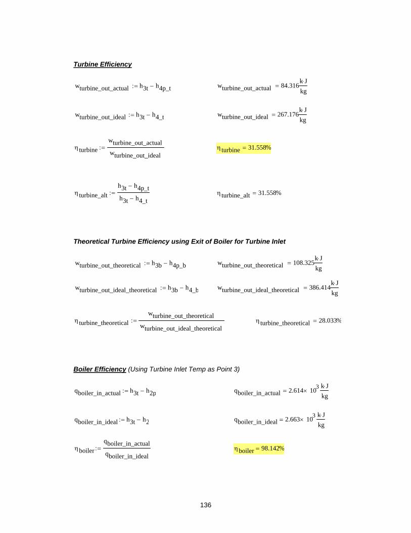
136
Turbine Efficiency
wturbine_out_actual h3t h4p_t−:= wturbine_out_actual 84.316k J⋅kg
=
wturbine_out_ideal h3t h4_t−:= wturbine_out_ideal 267.176k J⋅kg
=
η turbinewturbine_out_actualwturbine_out_ideal
:= η turbine 31.558%=
η turbine_alth3t h4p_t−
h3t h4_t−:= η turbine_alt 31.558%=
Theoretical Turbine Efficiency using Exit of Boiler for Turbine Inlet
wturbine_out_theoretical h3b h4p_b−:= wturbine_out_theoretical 108.325k J⋅kg
=
wturbine_out_ideal_theoretical h3b h4_b−:= wturbine_out_ideal_theoretical 386.414k J⋅kg
=
η turbine_theoreticalwturbine_out_theoretical
wturbine_out_ideal_theoretical:= η turbine_theoretical 28.033%=
Boiler Efficiency (Using Turbine Inlet Temp as Point 3)
qboiler_in_actual h3t h2p−:= qboiler_in_actual 2.614 103×
k J⋅kg
=
qboiler_in_ideal h3t h2−:= qboiler_in_ideal 2.663 103×
k J⋅kg
=
ηboilerqboiler_in_actualqboiler_in_ideal
:= ηboiler 98.142%=
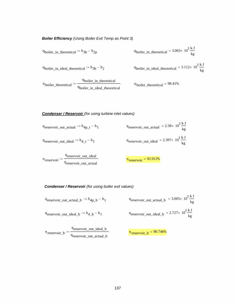
137
Boiler Efficiency (Using Boiler Exit Temp as Point 3)
qboiler_in_theoretical h3b h2p−:= qboiler_in_theoretical 3.063 103×
k J⋅kg
=
qboiler_in_ideal_theoretical h3b h2−:= qboiler_in_ideal_theoretical 3.112 103×
k J⋅kg
=
ηboiler_theoreticalqboiler_in_theoretical
qboiler_in_ideal_theoretical:= ηboiler_theoretical 98.41%=
Condenser / Reservoir (for using turbine inlet values)
qreservoir_out_actual h4p_t h1−:= qreservoir_out_actual 2.58 103×
k J⋅kg
=
qreservoir_out_ideal h4_t h1−:= qreservoir_out_ideal 2.397 103×
k J⋅kg
=
ηreservoirqreservoir_out_idealqreservoir_out_actual
:= ηreservoir 92.912%=
Condenser / Reservoir (for using boiler exit values)
qreservoir_out_actual_b h4p_b h1−:= qreservoir_out_actual_b 3.005 103×
k J⋅kg
=
qreservoir_out_ideal_b h4_b h1−:= qreservoir_out_ideal_b 2.727 103×
k J⋅kg
=
ηreservoir_bqreservoir_out_ideal_bqreservoir_out_actual_b
:= ηreservoir_b 90.746%=
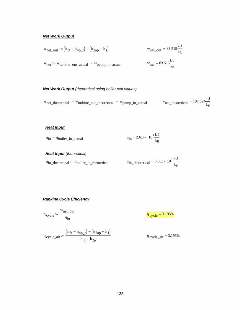
138
Net Work Output
wnet_out h3t h4p_t−( ) h2ap h1−( )−:= wnet_out 83.515k J⋅kg
=
wnet wturbine_out_actual wpump_in_actual−:= wnet 83.515k J⋅kg
=
Net Work Output (theoretical using boiler exit values)
wnet_theoretical wturbine_out_theoretical wpump_in_actual−:= wnet_theoretical 107.524k J⋅kg
=
Heat Input
qin qboiler_in_actual:= qin 2.614 103×
k J⋅kg
=
Heat Input (theoretical)
qin_theoretical qboiler_in_theoretical:= qin_theoretical 3.063 103×
k J⋅kg
=
Rankine Cycle Efficiency
ηcyclewnet_out
qin:= ηcycle 3.195%=
ηcycle_alth3t h4p_t−( ) h2ap h1−( )−
h3t h2p−:= ηcycle_alt 3.195%=

139
Rankine Cycle Efficiency (theoretical)
ηcycle_theoreticalwnet_theoreticalqin_theoretical
:= ηcycle_theoretical 3.511%=
ηcycle_theoretical_alth3b h4p_b−( ) h2ap h1−( )−
h3b h2p−:= ηcycle_theoretical_alt 3.511%=
Ideal Rankine Cycle Efficiency
wnet_ideal wturbine_out_ideal wpump_in_ideal−:= wnet_ideal 266.315k J⋅kg
=
wnet_out_ideal h3t h4_t−( ) h2a h1−( )−:= wnet_out_ideal 266.315k J⋅kg
=
qin_ideal qboiler_in_ideal:= qin_ideal 2.663 103×
k J⋅kg
=
ηcycle_idealwnet_idealqin_ideal
:= ηcycle_ideal 10%=
ηcycle_ideal_alth3t h4_t−( ) h2a h1−( )−
h3t h2−:= ηcycle_ideal_alt 10%=

140
Ideal Rankine Cycle Efficiency (theoretical)
wnet_ideal_theoretical wturbine_out_ideal_theoretical wpump_in_ideal−:=
wnet_ideal_theoretical 385.553k J⋅kg
=
wnet_out_ideal_theoretical h3b h4_b−( ) h2a h1−( )−:= wnet_out_ideal_theoretical 385.553k J⋅kg
=
qin_ideal_theoretical qboiler_in_ideal_theoretical:= qin_ideal_theoretical 3.112 103×
k J⋅kg
=
ηcycle_ideal_theoreticalwnet_ideal_theoreticalqin_ideal_theoretical
:= ηcycle_ideal_theoretical 12.388%=
ηcycle_ideal_theoretical_alth3b h4_b−( ) h2a h1−( )−
h3b h2−:= ηcycle_ideal_theoretical_alt 12.388%=
Comparison of Actual to Ideal
ηactual_to_idealηcycle
ηcycle_ideal:= ηactual_to_ideal 31.953%=
Comparison of Actual to Ideal (theoretical)
ηactual_to_ideal_theoreticalηcycle_theoretical
ηcycle_ideal_theoretical:= ηactual_to_ideal_theoretical 28.339%=

141
Carnot Efficiency
TC 296.99K:= TH_t 431.46K:= TH_b 644.78K:=
ηcarnot_t 1TC
TH_t−:= ηcarnot_t 31.166%=
ηcarnot_b 1TC
TH_b−:= ηcarnot_b 53.939%=
System Efficiency Compared to Carnot
ηrankine_to_carnot_tηcycle
ηcarnot_t:= ηrankine_to_carnot_t 10.252%=
ηrankine_to_carnot_bηcycle
ηcarnot_b:= ηrankine_to_carnot_b 5.924%=
System Efficiency Compared to Carnot (theoretical)
ηrankine_to_carnot_theoreticalηcycle_theoretical
ηcarnot_b:= ηrankine_to_carnot_theoretical 6.508%=

142
APPENDIX M
AUTOCAD DRAWINGS AND DIMENSIONING
OF
T-500
IMPULSE STEAM TURBINE
AND
GEAR TRAIN

143
Figure M.1: Detailed drawing for complete assembly of T-500 impulse steam
turbine and gear train.

144
Figure M.2: Detailed drawing of T-500 impulse steam turbine rotor (blades) ,
housing, and nozzle design.

145
Figure M.3: Detailed drawing for first section of gear train; bearing plates one, two,
and four, thrust plate, bearing cover, and high speed gear housing.

146
Figure M.4: Detailed drawing of bearing plate three, low speed gear housing, and
intermediate speed gear housing.

147
APPENDIX N
RECEIVER/BOILER
DETAILED DRAWINGS AND IMAGES
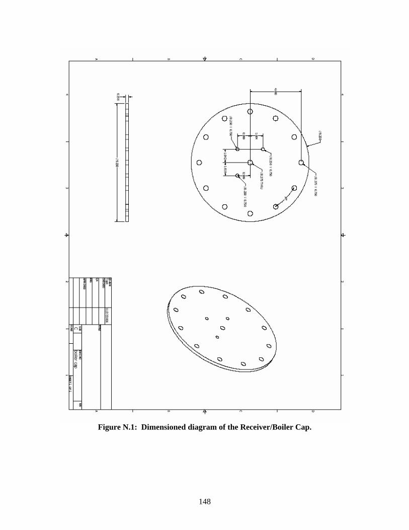
148
Figure N.1: Dimensioned diagram of the Receiver/Boiler Cap.
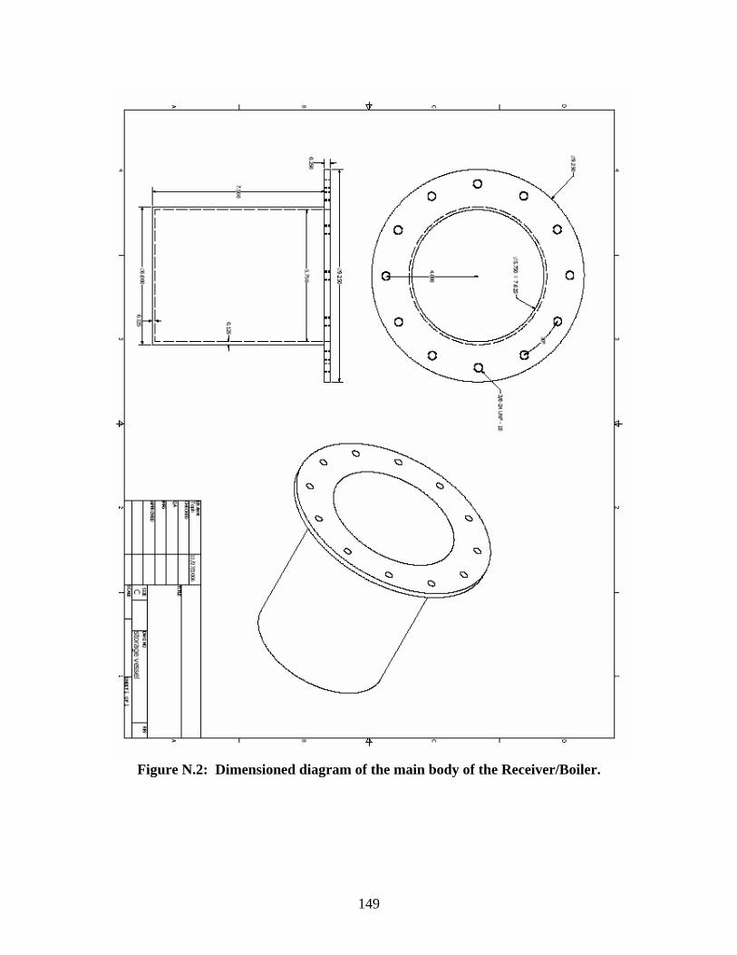
149
Figure N.2: Dimensioned diagram of the main body of the Receiver/Boiler.

150
Figure N.3: Dimensioned diagram of the outer coils contained within the receiver.

151
Figure N.4: Dimensioned diagram of the inner coils housed within the receiver.

152
Figure N.5: Dimensioned diagram of the water drum located in the receiver.

153
Figure N.6: a) Exploded ¾ view of receiver/boiler. b) ¾ view of assembled
receiver/boiler.
Figure N.7: Image of the actual receiver cap, inner and outer coils, and water drum
assembled.

154
Figure N.8: Main body of the receiver/boiler.
Figure N.9: Assembled receiver/boiler being heated on electric burner for initial
mixing of the draw salt thermal bath.
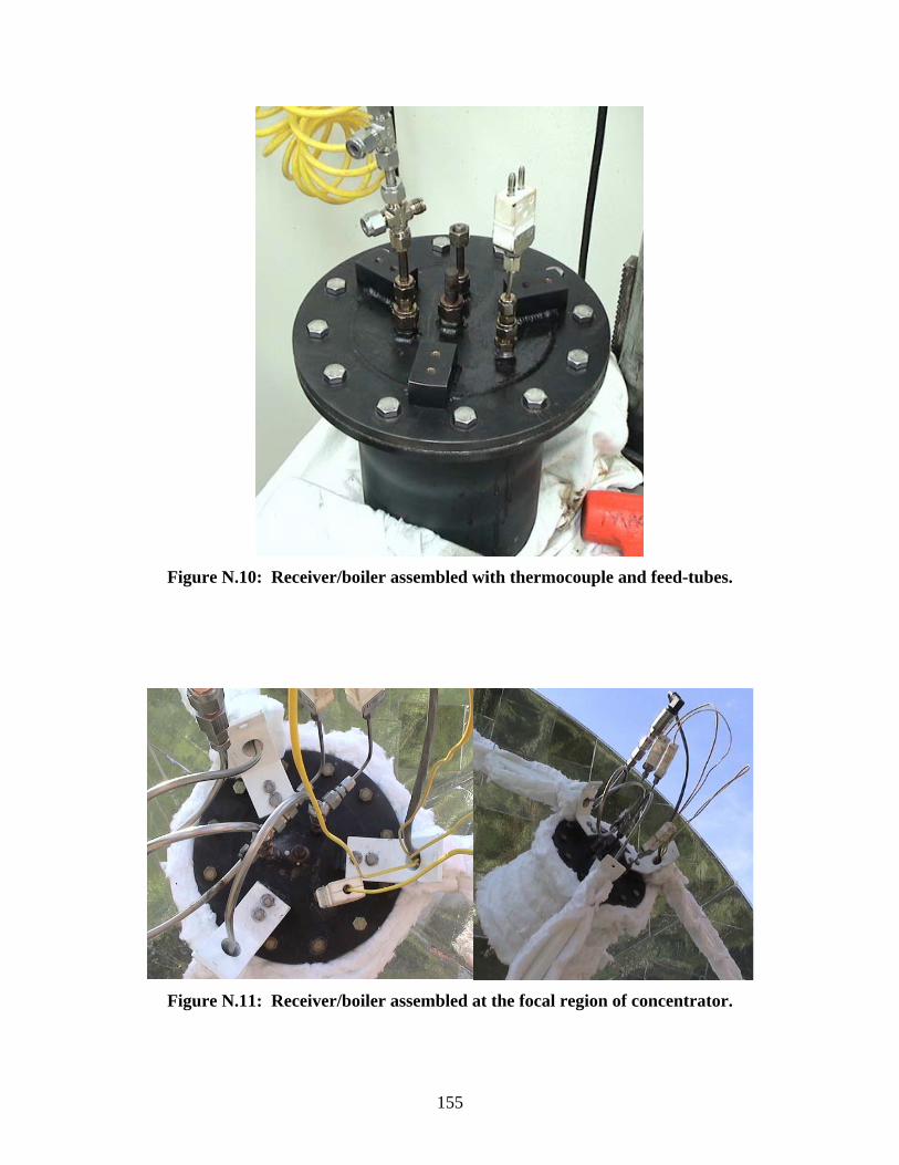
155
Figure N.10: Receiver/boiler assembled with thermocouple and feed-tubes.
Figure N.11: Receiver/boiler assembled at the focal region of concentrator.
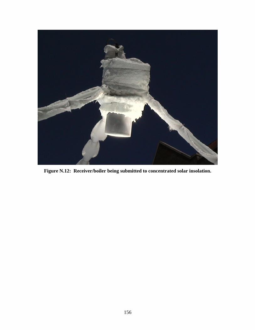
156
Figure N.12: Receiver/boiler being submitted to concentrated solar insolation.

157
APPENDIX O
SOLAR CHARGER CONTROLLER
ELECTRICAL DIAGRAM
Figure O.1: Diagram of the solar charger controller circuit board layout.

158
Figure O.2: Solar charger controller wiring schematic.

159
APPENDIX P
WINDSTREAM POWER LOW RPM PERMANENT
MAGNET DC GENERATOR
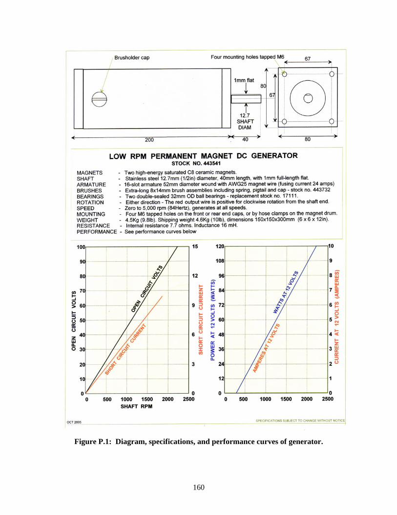
160
Figure P.1: Diagram, specifications, and performance curves of generator.


