Download - THE DETERMINANTS OF EXCHANGE RATE IN NIGERIA

THE DETERMINANTS OF EXCHANGE RATE IN NIGERIA BY UDOYE, RITA A. PG/M.Sc/ 07/43765
BEING A RESEARCH PROJECT SUBMITTED TO THE DEPARTMENT OF
ECONOMICS, UNIVERSITY OF NIGERIA, NSUKKA IN PARTIAL
FULFILLMENT OF THE REQUIREMENTS FOR THE AWARD OF M.Sc IN
ECONOMICS
NOVEMBER, 2009.

i
TITLE PAGE THE DETERMINANTS OF EXCHANGE RATE IN NIGERIA.

ii
APPROVAL PAGE THE DETERMINANTS OF EXCHANGE RATE IN NIGERIA BY UDOYE, RITA A. PG/ M.Sc/ 07/ 43765 THIS PROJECT IS APPROVED BY THE DEPARTMENT OF ECONOMICS, UNIVERISTY OF NIGERIA, NSUKKA. __________________ _____________________ Prof. C.C Agu Prof. C.C Agu Supervisor Head of Department ____________________ External Examiner

iii
DEDICATION. This work is dedicated to God Almighty for His infinite mercies upon me. I also
dedicate this work to my husband, Mr L.O Udoye and to my children – Onyii,
Nelo, Chukwudi, Chibuzo, Nnemeka and Ogoo. May the blessings of the Lord
continue to abide with you all.

iv
ACKNOWLEDGEMENT I am very grateful to God for successful completion of this program.
I also acknowledge the help of my supervisor, Prof.C.C.Agu, whose advice,
guidance and understanding contributed immensely to the success of this work.
I am also greatly indebted to my brothers and sisters - Mary, Cordy, Vitus, Emeka
and my nephew - Tochukwu and many others. May God bless you all in Jesus
name, Amen.
Udoye, R.A. U.N.N.
v
ABSTRACT
The study examines the determinants of real exchange rate in the recent years in
Nigeria over the period of 1970 to 2006 using the Nigerian time series data.
Following literature, we identified the potential determinants of real exchange rate
as lag of real exchange rate, real interest rate, inflation rate, trade openness and
real gross domestic product. After examined the time series characteristics of the
data with Augmented Dickey-Fuller (ADF) unit roots test of stationarity and
Engle-Granger procedure for co-integration test, we applied Auto-regressive
Distributed Lag Model (ARDL-ECM). The result suggests that one year past value
of real exchange rate and immediate past value of trade openness are the major
determinants of real exchange rate in Nigeria. The result further indicates that
there is evidence of long run relationship between real exchange rate and two
explanatory variables (gross domestic product growth rate and trade openness).

vi
TABLE OF CONTENT TITLE PAGE ii APPROVAL PAGE iii DEDICATION iv ACKNOWLEDGEMENT v ABSTRACT vi TABLE OF CONTENT vii LIST OF TABLES ix CHAPTER ONE: INTRODUCTION 1 1.1 BACKGROUND INFORMATION 1 1.2 STATEMENT OF THE PROBLEM 3 1.3 OBJECTIVES OF THE STUDY 5 1.4 STATEMENT OF HYPHOTHESIS 5 1.5 JUSTIFICATION OF THE STUDY 6 1.6 SCOPE AND LIMITATION OF THE STUDY 6 CHAPTER TWO: LITERATURE REVIEW 7 2.0 THEORETICAL BACKGROUND 7 2.1 MODELS OF EXCHANGE RATE DETERMINATION 7 2.1.1 TRADITIONAL FLOW MODEL 7 2.1.2 THE PORTFOLIO BALANCE MODEL 8 2.1.3 THE MONETARY APPROACH 8 2.1.4 PURCHASING POWER PARITY (PPP) 9 2.1.5 BALANCE OF PAYMENTS APPROACH 9 2.1.6 EXCHANGE RATE REGIMES 10 2.1.7 CRAWLING PEG 10 2.1.8 ADJUSTABLE PEG EXCHANGE RATE 11 2.1.9 TARGET ZONE 12 2.1.10 CURRENCY PEG 12 2.2 BRIEF THEORETICAL REVIEW 13 2.3 AN OVERVIEW OF NAIRA EXCHANGE RATE MANAGEMENT 16 2.4 EMPIRICAL REVIEW 21 2.5 LIMITATION OF PREVIOUS STUDIES 28 2.6 EXCHANGE RATE MOVEMENTS IN NIGERIA 1975-2006 29

vii
CHAPTER THREE: METHODOLOGY 31 3.1 THE MODEL 31 3.2 MODEL SPECIFICATION 31 3.3 ESTIMATION PROCEDURE 32 3.4 UNIT ROOT TEST 33 3.5 CO-INTEGRATION TEST 34 3.6 TECHNIQUES OF RESULTS EVALUATION 35 3.7 MODEL JUSTIFICATION 35 3.8 DATA SOURCES 36 3.9 ECONOMETRIC SOFTWARE 36 CHAPTER FOUR: PRESENTATION AND INTERPRETATION OF RESULT 37 4.1 OVERVIEW 37 4.2 CO-INTEGRATION TEST 38 4.3 PRESENTATION OF DYNAMIC ECM MODELING OF REXCH RESULT 38 4.4 INTERPRETATION OF RESULT 39 4.5 COEFFICIENT OF DETERINATION R2 41 4.6 TEST OF AUTOCORRELATION 41 4.7 F-TEST 41 4.8 TESTOF MULTICOLLINEARITY 42 CHAPTER FIVE: SUMMARY, CONCLUSION AND POLICY RECOMMENDATION 43 5.1 SUMMARY AND CONCLUSION 43 5.2 POLICY RECOMMENDATION 44 5.3 CONCLUSION 46 REFERENCES 48 APPENDIX

viii
LIST OF TABLES 4.1 UNIT ROOT TEST 37 4.2 CO-INTEGRATION RESULT 38 4.3 RESULT SUMMARY 38 4.4 CORRELATION MATRIX 42
1
CHAPTER ONE
INTRODUCTION
1.1 Background Information
The exchange rate is the rate at which one currency is exchanged for another. It is
the price of one currency in terms of another currency ( Jhingan, 2005). Exchange
rate is the price of one unit of the foreign currency in terms of the domestic
currency. The debate over what determines the choice of exchange rate regimes
has continued unabated over some decades now. Friedman (1953) argued that in
the presence of sticky prices, floating rates would provide better insulation from
foreign shocks by allowing relative prices to adjust faster. His popular support for
floating exchange rate stipulates that in the long run the exchange rate system does
not have significant real consequences. His reasoning is that the exchange rate
system is ultimately a choice of monetary regimes. In the end, monetary policy
does not matter for real quantities, but in the short run it does. While Mundell’s
(1963) posits that in a world of capital mobility, optimal choice of exchange rate
regime should depend on the type of shocks hitting an economy: real shocks would
call for a floating exchange rate, whereas monetary shocks would call for a fixed
exchange rate.
�
Traditionally, it has been argued that a country’s optimal real exchange rate is
determined by some key macroeconomic variables and that the long-run value of
the optimal real exchange rate is determined by suitable (permanent) values of
these macroeconomic variables (Williamson, 1994). Incidentally, since the fall of
Bretton-Woods system in 1970s and the subsequent introduction of floating

2
exchange rates, the exchange rates have in some cases become extremely volatile
without any corresponding link to changes in the macroeconomic fundamentals.
This however has led to higher interest in exchange rate modeling as the question
of exchange rate determination reveals to be one of the most important problems
on theoretical field of monetary macroeconomics.
�
There are different types of exchange rate regimes practiced all over the world;
from the extreme case of fixed exchange rate system to a freely floating regime.
Practically, countries tend to adopt a combination of different regimes such as
adjustable peg, crawling peg, target zone/crawling bands, and managed float,
whichever that suits their peculiar economic conditions. For instance, exchange
rate managements in Nigeria has witness different significant changes over the past
four decades. Nigeria maintained fixed exchange rates from 1960 till the
breakdown of the Bretton Woods Monetary System in the early 1970s. Between
1970 and mid 1980 Nigeria exchange rate policy shifted from fixed exchange rate
to a pegged arrangement and finally, to the various types of the floating regime
since 1986 following the adoption of the Structural Adjustment Programme (SAP)
(see Sanusi, 2004).
A regime of managed float, without any strong commitment to defend any
particular parity, has been the predominant characteristic of the floating regime in
Nigeria since 1986. The changes from the different regimes are not peculiar to the
Naira as the US dollar was fixed in gold terms until 1971 when it was de-linked
and has since been floated. The fixed exchange rate regime induced an
overvaluation of the naira and was supported by exchange control regulations that
engendered significant distortions in the economy. That gave vent to massive
importation of finished goods with the adverse consequences for domestic

3
production, balance of payments position and the nation’s external reserves level.
Moreover, the period was bedeviled by sharp practices perpetrated by dealers and
end-users of foreign exchange. These and many other problems informed the
adoption of a more flexible exchange rate regime in the context of the SAP,
adopted in 1986 (Sanusi, 1988).
1.2 Statement of the Problem
Foreign exchange is said to be an important element in the economic growth and
development of a developing nation. Foreign exchange policies influence the
economic activities and to a large extent, dictate the direction of the macro-
economic variables in the country. The mechanism of exchange rate determination
are different systems of managing the exchange rate of a nation’s currency in
terms of other currencies and this should be properly done in a way that will bring
about efficient allocation of scarce resources so as to achieve growth and
development. Jhingan (2005) posited that to maintain both internal and external
balance, a country must control its exchange rate.
Optimal exchange rate policy is designed to obtain real exchange rate (RER) that
maintains both internal and external balance (Agu, 2002). The concept of real
exchange rate comes from a realization that the observable nominal exchange rate
movements, result from both price changes and inflation rate changes in trading
economies. When the real exchange rate is optimal, domestic producers of tradable
goods can compete internationally; imports are not artificially cheaper than
comparable domestic alternatives. Exporters also are not disadvantaged by the
exchange rate, when the real exchange rate is right (Maciejewski, 1983). What
determines the exchange rate regime for an open economy is one of the oldest
issues in international economics. The single most influential idea in this context

4
has been the Mundellian prescription that if shocks facing the country are mostly
monetary then fixed exchange rates are optimal whereas flexible rates are optimal
if the shocks are mostly real (Amartya et al.2004). The key friction underlying
Mundell’s results was the assumption of sticky prices in the goods market. Since
the fall of Bretton-Woods system in 1970s and the subsequent introduction of
floating exchange rates, the exchange rates have in some cases become extremely
volatile without any corresponding link to changes in other macroeconomic
variables. Nigeria’s exchange rate changes have been a subject of debate among
policy makers, concerned monetary authorities and academics because of the
recognition of the vital role exchange rate regime plays in the achievement of
sustainable growth. Government and monetary authorities in Nigeria, over the
years have done a lot of work in the area of finding the appropriate exchange rate
management, given the peculiarities of the economy. Since the adoption of the
Structural Adjustment Programme in 1986, Nigeria has adopted different types of
exchange rate regimes, ranging from floating exchange rate regimes to
fixed/pegged regimes.
However, maintaining a realistic exchange rate for the naira in Nigeria is very
crucial, given the structure of the economy. Sanusi (2004) opined the importance
of maintaining a realistic exchange rate for naira, and also the need to minimize
distortions in production and consumption, increase the inflow of non-oil export
receipts and attract foreign direct investment. This is expected to ensure that the
naira is not overvalued in real terms, and that the external sector remains
competitive. Nigeria in 1960 and in the early 1970s, maintained fixed exchange
rates. Between 1970 and mid 1980 Nigeria exchange rate shifted from fixed
exchange rate to a pegged arrangement and since the introduction of Structural
Adjustment Programme in 1986 till date Nigeria has adopted various types of

5
floating exchange regime (Sanusi 2004). The quest for a realistic naira exchange
rate made the Central Bank of Nigeria (CBN) in the time past to employ the
Purchasing Power Parity (PPP) model as a guide to gauge movements in the
nominal exchange rate and to determine deviations from the equilibrium exchange
rate. Although the PPP as a relative price does not provide clear criteria for
choosing a base period, and is generally criticized for its insensitivity to short-term
policy actions, it nonetheless, provides a reasonable framework for a comparative
analysis of trading partners’ performances. Nigeria, having adopted various types
of exchange rate mechanism over the years with Dutch Auction System (DAS)
being the latest and still the exchange rate did not maintain both internal and
external balance. Thus, the ultimate questions which this research seeks to answer
are: what determines exchange rate in Nigeria? Again, is there any long run
relationship between the exchange rate and its identified determinants in Nigeria?
1.3 Objectives of the Study
The general objective of this study is to investigate which of the macroeconomic variables best determine the real exchange rate in Nigeria. Specifically, the study will find out: 1. The determinants of exchange rate in Nigeria.
2. If there is any long run relationship between the exchange rate and its
identified�determinants in Nigeria.
1.4 Statement of Hypothesis
1. The determinants exchange rate in Nigeria is unknown?
2. There is no long run relationship between the exchange rate and its identified
determinants in Nigeria?
6
1.5 Justification of the Study
The policy thrust of the NEED document is to use the retail Dutch Auction System
to determine the nominal exchange rate regime, and adopt a wholesale Dutch
auction in the medium to long term (NEED 2004). This is in view of the fact that
the overall goal of monetary policy remains price and exchange rate stability.
Thus, economic relevance of studying the determinants of real exchange rate need
not be overemphasized. This study is imperative given the recent efforts by
monetary authorities in Nigeria to revive the economy through the financial sector
reform which among other things sought to maintain stability in exchange rate.
Consequently, this study will assist the nation’s economic planners in their
economic development planning. Specifically, the outcome of this study would
provide a basic understanding of the dynamics of exchange rate and the key
macroeconomic variables in Nigeria and it also contribute to knowledge.
1.6 Scope and Limitation of Study
This study shall cover the period of 1970-2006; a sample size of 36 years is long
enough for time series analysis. The choice of this period is largely informed by
data availability, and also due to the fact that Nigerian economy has practiced
different types of exchange rate regimes within the given period.
7
CHAPTER TWO
LITERATURE REVIEW
2.0 Theoretical Background
Exchange rate is the rate at which one country’s currency is exchanged for the
currency of another country (Dornbusch, 2004). It can also be defined as the price
of one country’s currency relative to other countries’ currency. While, Mankiw,
(1997) define it as the price at which exchange between two countries take place.
How to determine the exchange rate is issue that has taken the centre stage of
monetary and international economics. Monetary policy authority in Nigeria is
faced with the problems of having a stable and realistic exchange rate which is in
consonance with other macroeconomic fundamentals. This is because exchange
rate instability can have serious adverse consequences on prices, investments and
international trade decisions. A realistic exchange rate is one that reflects the
strength of foreign exchange inflow and outflow, the stock of reserves as well as
ensuring equilibrium in the balance of payments that is consistent with the cost and
price levels of trading partners (Ojo, 1998).
2.1 Models of Exchange Rate Determination
In general, three models theoretical foundations of exchange rate determination
exist; they include the traditional flow, the portfolio balance and the monetary
models of exchange rate
2.1.1 Traditional Flow Model
This model posits that exchange rate is simply determined by the market flow of
demand and supply of foreign exchange. Thus, there is equilibrium when the
supply equals the demand for foreign exchange. The model assumes that two basic

8
variables interact to determine the exchange rate. The variables are: relative
income and interest rate differential. This is justified since foreign demand for
domestic goods is a function of foreign income and vice versa, and also asset
demand depends on the difference between domestic and foreign interest rates.
2.1.2 The Portfolio Balance Model
This approach to exchange rate determination conceptualizes exchange rate as the
result of the substitution between money and financial assets in the domestic
economy and the substitution between domestic and foreign financial assets (CBN,
1998). Macdonald and Taylor (1992) posited that an exchange rate is determined
at least in the short-run by the supply and demand in the markets for wide range of
financial assets would not be automatic. This is an asset pricing view of the
exchange rate. The idea is that agents have a portfolio choice decision between
domestic and foreign assets. Those instruments (either money or bonds) have an
expected return that could be arbitraged. This arbitrage opportunity is what
determines the process of the exchange rate (Dornbusch, 1988).
2.1.3 The Monetary Approach
The shortfalls of the portfolio balance theory led to the development of the
monetary approach. This approach is based on the importance of money as a unit
of exchange, thus, it visualizes exchange rate as a function of relative shift in
money stock, inflation rate and domestic output, between a country and a trading
partner economy. Frankel (1978) posits that this model of exchange rate
determination attains equilibrium when existing stocks of money in the two
countries are willingly held. The monetary approach, under the flexible exchange
rate can be presented in two forms the monetary approach or the asset market
approach, and it emphasized on the role of money and other assets in determining

9
the exchange. Obioma (2000) holds the view that asset market or monetary
approach attributes variation in exchange rate essentially to income and expected
rates of return as well as to other factors that influence the supplies of and demands
for the various national monies. Thus, based on the fact that supply and demand for
monies is determined by the level of income, the monetary model postulates three
basic determinants of exchange rate as follows: relative money supplies, relative
income and interest rate differentials.
2.1.4 Purchasing Power Parity (PPP)
The purchasing power parity approach to the exchange rate determination was, and
continues to be, a very influential way of thinking about the exchange rate. The
PPP posits that the exchange rate between two currencies would be equal to the
relative national level prices. The PPP derives from the assumption that in the
world there exists the "law of one price". This law states that identical goods
should be sold at identical prices. (Note this assumption not law). The law of one
price implies that exchange rates should adjust to compensate for price differentials
across countries (Hoontrakul 1999). In other words, if we are in a bread-world
(only bread exists), and a bread is sold in US at 1 Dollar, and the same bread is
sold in Nigeria at 150 naira, then the exchange rate has to be 150 naira per Dollar.
2.1.5 Balance of Payments Approach
This approach of exchange rate determination is that there exists internal and
external equilibrium. The internal equilibrium assumes that there is full
employment: in it there is natural rate of unemployment. Or in other words, the
unemployment is such that there are no pressures to change real wages. The
external equilibrium refers to equilibrium in the balance of payments. This
approach explains permanent deviations of PPP. The main problem with this

10
approach is that in general it is extremely difficult to determine what is the exact
natural rate of unemployment, or the exchange rate that is consistent with
equilibrium of the external accounts. However, the model will determine where the
exchange rate has to converge to; however, it provides very little guidance to the
short term fluctuations (Hoontrakul 1999).
2.1.6 Exchange Rate Regimes
The options available to countries for adopting a particular exchange rate regimes
range from floating arrangements at one extreme to firmly fixed arrangements at
the other extreme, with the remaining regimes falling on a continuum in between.
These include pegs, target zones, and fixed but adjustable rates. As exchange rate
management have a defining goal of exchange rate stability, the fixed exchange
rate regime and its variants are more relevant. A fixed exchange rate system is one
in which exchange rates are maintained at fixed levels. Each country has its
currency fixed against another currency, and it is seldom changed. For example,
Nigeria maintained fixed exchange rates from the time of attainment of political
independence in 1960 till the breakdown of the Bretton Woods Monetary System
in the early 1970s. There are two major reasons why fixed exchange rates are
appealing. They are to promote orderliness in foreign exchange markets and
certainty in international transactions. Some of the variants of fixed exchange rates
are as follows:
2.1.7 Crawling Peg
This exchange rate arrangement is a middle course between fixed and flexible
exchange rates. It is appropriate for countries that have significant inflation
compared with their trading partners, as has often been the case in Latin America.

11
Under the crawling peg, the government fixes the exchange rate on any day but
over time adjusts the rate in a pre-announced fashion, taking into consideration the
inflation differentials between it and its major trading partners. Essentially, the peg
can be either passive, meaning that the exchange rate is altered in light of past
inflation, or active, whereby the country announces in advance the exchange rate
adjustments it intends to make. The advantage of this peg is that it combines the
flexibility needed to accommodate different trends in inflation rates between
countries while maintaining relative certainty about future exchange rates relevant
to exporters and importers. The disadvantage is that the crawling peg leaves the
currency open to speculative attack because the government is committed on any
one day or over a period to a particular value of the exchange rate.
2.1.8 Adjustable Peg Exchange Rate This refers to the system in which a national currency is pegged to a key currency,
for example, the U.S dollar, but the level of the peg could be changed occasionally,
albeit within a narrow band. This exchange rate regime features a strong exchange
rate commitment, and its adherents before the currency crises of the mid- and late
1990s, included Brazil, Mexico and Thailand. In these emerging market
economies, where capital mobility increased steadily during the 1970s and 1980s
and up to a high point in the 1990s, the authorities had difficulties in maintaining
the peg (Corden, 2001). However, it is still workable for countries that have low
capital mobility either because they are not integrated with the capital markets (like
some very poor countries) or because they have effective capital controls (e.g.
China).
12
2.1.9 Target Zone This is a compromise between floating rates and fixed but adjustable rates and is a
popular regime. Under it, a central rate that can be fixed, crawling or flexible is
surrounded by a band within which the central rate is permitted to float. It allows
for flexibility among a country’s policy objectives. It is also said to prevent
extreme movements in the exchange rate.
2.1.10 Currency Peg In a currency peg a local currency is pegged to an external currency, e.g., that of a
dominant trading partner or to a basket of currencies, with weights reflecting the
shares of the countries in foreign trade. Pegging to a single currency may yield a
number of advantages, one of which is the reduction in the exchange rate
fluctuations between the focus country and the country to which it is pegged. This
facilitates trade and capital flows between the two countries. One major weakness
of the single currency peg, however, is that where the currency is pegged to a
floating currency, e.g., the dollar, the local currency will float along with the dollar
vis-à-vis other currencies. Another disadvantage is that movements in the exchange
rate in relation to the currencies of other countries may interfere with domestic
macroeconomic policy objectives.
In an attempt to stabilize its effective exchange rate the developing country may
peg its currency to a basket of currencies. Often this entails the weighted average
of several currency values, the resulting exchange rate being total trade-weighted,
export weighted or import-weighted. One major advantage of pegging to a basket
is that a country may be able to avoid large fluctuations in its exchange rate with
respect to several trading partners’ currencies. Consequently, it is able to stabilize

13
its nominal effective exchange rate. Another advantage is that the system results in
the reduction of price instability which arises from exchange rate changes.
However, one major disadvantage of the basket peg is the determination of the
exchange rate without reference to the domestic policies of the pegging authorities.
Another is that a basket-weighted exchange rate, which, by definition, moves
against all major currencies, might reduce confidence on the part of foreign
investors and reduce capital inflows.
2.2 Brief Theoretical Review Given the potential impact of exchange rate on inflation prices, investment,
balance of payment, and interest rate, the issue of the determination of optimal
exchange rate becomes imperative for the successful implementation of
development programmes in the country. Chuka, (1990) argues that the objectives
of exchange rate policy are to increase output and its optimal distribution. A
necessary condition for the achievement of the above objectives is that the
exchange rate should be stable as possible. According to him, stability permits
viability of the rate in response to changes in relative prices, international terms of
trade and growth factors.
Exchange rate policy involves choosing an exchange rate system and determining
the particular rate at which foreign transaction will take place. Exchange rate
policy affects growth by determining capital flow, foreign investment and external
balance for most developing countries. The inadequacy of foreign exchange
constitutes a bottle neck in the process of development. In the course of
development, the rate of growth of national output and the demand for imports
tend to exceed export based capacity. Therefore, there is a conflict between
accelerating internal development and maintaining external balance. This conflict

14
is resolved by a realistic exchange rate policy. Exchange rate policy by devaluation
or over-valuation has an implication for an economy. Devaluation help to improve
the external competitiveness either through contraction in imports or expansion in
exports and this influences both consumption and investment decision. Over-
valuation of foreign exchange exacerbate external borrowing, balance of payment
disequilibrium and the distortion of the economy, while under valuation results in
income distortion detrimental to labour, trade, current account surpluses, standard
of living and the growth of the economy (Sodersten, 1997).
The basic element of efficient exchange rate system is the assumption that
exchange rate reflects the relative productivity of an economy (Obadan, 2003). In
the long-term, the devalued Naira protects domestic industries, encourages
domestic production, reduction in the cost of imported raw materials and makes
domestically produced goods competitive.
Several factors influencing the choice of a particular exchange rate regime in a
country, a major consideration is the internal economic conditions or
fundamentals, the external economic environment and the effect of various random
shocks on the domestic economy. Thus, countries like Nigeria which are
vulnerable to unstable internal financial conditions and external shocks, (including
terms of trade shocks, and excessive debt burden), which require real exchange
rate depreciation, tend to adopt a regime which ensures greater flexibility. Overall,
there is a general consensus that a fixed exchange rate regime is preferred if the
source of macroeconomic instability is predominantly endogenous. Conversely, a
flexible regime is preferred if disturbances are predominantly exogenous in nature.
It is, nevertheless, becoming increasingly recognized that whatever exchange rate
regime a country may adopt, the long-term success depends on its commitment to
15
the maintenance of strong economic fundamentals and a sound banking system
(see Sanusi, 2004).
Meese, and Rogoff (1990) maintains that the floating exchange rate was adopted in
developing countries from 1973 and the question of whether exchange rate
changes/uncertainties have independent adverse effect on transaction of a country
have attracted a lot of literature. According to them, the introduction of adjustment
programmes by many of these countries and the attendant liberalization of
exchange rates have brought the discussion of this work further into global focus.
Economists are divided over whether government’s arguments for managing
exchange rate rest on three points firstly, the government can determine the
fundamental equilibrium exchange rate. Secondly, floating exchange rate has been
too volatile. Thirdly under floating exchange rate currencies can become
significantly over-valued or undervalued. The first and third points are related.
Williamson, (1994) proclaim that the supporters of floating exchange rates points
out that exchange rate volatility may or may not have adverse effect on favorable
terms of trade depending on it’s effect on import. Therefore exchange rate
volatility or fluctuation can be positive or negative.
Taylor, (1995) in his work stated quite categorically what became known as
purchasing power parity theory that the value of a foreign currency in terms of
another depends mainly on the relative purchasing power of the two currencies in
their respective countries. In other words, the exchange rates settles at the level
which make purchasing power of a given unit of currency the same in what ever
country it is spent. He argues further that the theory fails in some areas like a
16
change in the exchange rate may originate in factor independent of price level.
Therefore the purchasing power parity is not a complete explanation of what
determines exchange rate but this does not mean that the theory has no value.
Krueger, (1983) maintains that in a completely free exchange market, exchange
rate would fluctuate freely in response to varying demand for the different
currencies; with fluctuating demand for currencies. Large savings in foreign
exchange rate could be expected especially since capital movement affect
exchange rate as directly as do merchandise export and imports. On the other hand,
as long as supply and demand for various currencies remains responsibly in
balance, stable exchange rate would prevail under free exchange markets. In
addition, Krueger, (1983) argues that how the exchange is determined depends on
whether the rate is a fixed exchange rate or floating exchange rate. A fixed
exchange rate is an exchange rate that is set by government decree or intervention
within a small range of variation. A floating exchange rate is freely determined by
the interaction of supply or demand.
2.3 An Overview of Naira Exchange Rate Management
Before the introduction of Structural Adjustment Programme (SAP) in 1986, the
naira exchange rate remained fixed. That is, the rate was fixed vis-à-vis the US and
UK’s dollar and pound sterling respectively. Although this was in line with the
global practice on exchange rate determination then, the system was found to be
fraught with high distortions leading to inefficiencies and misallocation of
resources. It observed that exchange rate in Nigeria did not become a policy
instrument until late 1988 like other developing countries. The Naira exchange rate
was pegged initial to the British pound sterling and subsequently to the United
States dollar as part of global exchange rate management under the Bretton woods

17
system. Here in, the naira exchange rate could be changed only in response to a
prolonged disequilibrium.
The Nigeria pound has its parity defined in June 1962 in terms of gold at one
Nigerian pound to 2.48828 grams for fine gold. From that time to August 14, 1971,
the exchange rate of the Nigerian pound of the use dollar was determined by its
gold parity. The Naira replaced the pound as Nigerian currency in 1973, and its par
value was set at half that of the pound. Hence the exchange rate against the dollar
became US $ 1.52 to the Naira. Within a month of this the US dollar was
devalued by 10 percent and Nigeria suit with a 10 percent matching devaluation,
thereby maintaining the existing Naira-dollar rate. During most of 1973, the
anchor currencies, the dollar and sterling weakened considerably, sustained
weakness brought into sharp focus the dilemma, inherent in the method of
determining the exchange rate of the Nigerian currency.
However, in September, 1986, the Second Tier Foreign Exchange market (SFEM)
began as a dual exchange rate system which produced the official first tier rate and
the SFEM or free market rate. The former was administratively determined and
gradually depreciated. It applied to a few official international organizations the
free market rate which applied to other transactions. The free market rate which
applied to other transactions was determined by the market forces of demand
supply within the framework of a foreign exchange auction system. The essence
of the dual exchange rate system was to avoid a deliberate uniform and sizeable
devaluation of the Naira but to allow it to depreciate in the SFEM while at the
same time the monetary authorities continued a downward adjustment of the first
tier rate until the two rates converge to produce a realistic exchange rate.

18
This convergence which Ojamenaye (1991) has described was achieved on July 2,
1987 at an exchange rate of N3.74: $1.00. With this development, the first tier
market was abolished and unified foreign exchange market (FEM) with a single
rate that came into being. The FEM also embraced the autonomous market, which
was allowed to develop. The autonomous segment of the FEM was expected to be
competitive with the parallel foreign exchange market and thus be attractive to
exporters to repatriate their proceeds.
The introduction of the autonomous market led to the existence of three exchange
rates - FEM, rate autonomous and the parallel market rate which failed to show any
tendency toward convergence. And as Akinmoladun (1990) has argued the merger
of the first tier rate and the SFEM rate was more technical than real as shortly after
the gap between the auction rate and those of the autonomous market rates began
to grow at one point, there was more than 50 percent differential between the two
rates and this became a source of concern for the monetary authorities. The price
differential had the effect of making the auction funds sort of subsidized.
The operations of the autonomous market later became destabilizing arising from
the tendency towards high arbitrage premium and accusations of authorized dealers
of diverting official funds making substantial gains effortlessly (Ojo, 1991). Other
malpractices also developed as the market officials or authorized dealers were
accused of corruption and allocation of foreign exchange to favored customers.
In the light of these, the autonomous market was merged with the official segment
in January 1989 and the Inter-Bank Foreign Exchange Market (IFEM) was
introduced. The IFEM entailed a daily bidding system under which the central
Bank injected official funds into the market by way of direct sales to the banks as
and when funds were available. Various but specific methods were used (single or

19
combined) to determine rates. The daily bidding system was characterized by
spurious demands for foreign exchange and it came to an end on the 13th
December, 1990. The following day, the CBN reintroduce the Dutch Auction
System (DAS) on a weekly basis.
The system continued throughout 1991. It may be recalled that the Dutch auction
system was first introduced in 1988, but was later replaced by IFEM. The DAS
was originally introduced to enhance professionalism in the FEM and prevent
outrageous rate which invariably led to the continued depreciation of the naira.
The system did not achieve this goal. For example, the naira showed heavier
deprivation in 1991 compared to the relative stability of the exchange rate in 1990
(Obadan, 1992). The exchange rate management system appeared to have been
predicated on various methods that are yet to achieve the desired goal. Not only
has there been a metamorphosis of the institutional framework from SFEM to FEM
to IFEM, there have been frequent changes in the operational guidelines. Besides
the Dutch Auction System, the market has experimented among which various
techniques and operational procedures among which are the average and marginal
exchange rate determination or fixed methods, the weekly, fortnight and daily
bidding system.
In January 1999, Nigeria’s dual exchange rate regime was abandoned as the
official N22 to a dollar exchange rate was scrapped. Prior to then, the official rate
co-existed with the rates on the Autonomous Foreign Exchange Market (AFEM)
and was used for selected government transactions including external debt service.
From then, the prevailing rate on the AFEM applied to all foreign exchange
transactions. The elimination of the dual exchange rate system introduced
uniformity of price in foreign exchange transactions and eliminated the arbitrage

20
opportunities created by having an overvalued official rate side-by-side with a
market determined rate. It also introduced more transparency into government
financial transactions as only the President previously had the right to determine
which transactions were to be conducted at the official rate. In October 1999, a
daily Inter-Bank Foreign Exchange Market (IFEM) replaced the AFEM. Under the
IFEM, the CBN monopoly on the supply of foreign exchange was removed as oil
exploration and producing companies were allowed to sell foreign exchange
directly to banks rather than through the CBN. The CBN however remains the
principal supplier of foreign exchange in the market and exerts considerable
influence on the determination of the exchange rate. In July, 2002, Nigeria
reintroduced a bi-weekly Dutch auction system (DAS) as an operational system for
its foreign exchange market to replace the inter bank foreign exchange market
(IFEM).
The DAS is a method of exchange rate determination through auction where
bidders pay according to their bid rates where the ruling rate is an arrived at with
the last bid rate that clears the market. In short, contrary to the old IFEM system,
where supply of currency was elastic at some given rate, take or leave some
allowance for depreciation when demand was perceived to be too large, under the
DAS the exchange rate is mainly determined by bids made by commercial banks
on behalf of their clients. So the move back to a DAS indicates that Nigeria seems
to be wishing for more, rather than less, flexibility in the exchange rate and leads
one to think that Nigeria appears to be opting for the last monetary regime
solution: stable prices and a freely floating exchange rate.

21
2.4 Empirical review
Jimoh, (2006) examines the Nigerian data from 1960 to 2000 to see what support it
provides for traditional theory of real exchange rate. He used the well-known
Johanson’s (1992) methods for estimating models whose variables are non-
stationary but co integrated, the study found that the decisive trade liberalization
programme of 1986 – 87 led to about 13 per cent depreciation in the Nigerian real
exchange rate and made the real rate more responsive to changes in its terms of
trade. He also found out that less decisive changes in trade regime produced no
significant changes in the real exchange rate.
Shehu and Aliyu (2006) estimate the long run behavioral equilibrium exchange
rate in Nigeria. They used quarterly data from 1984Q1 to 2004Q4 and derive a
Behavioral Equilibrium Exchange Rate (BEER) and a Permanent Equilibrium
Exchange Rate (PEER). Regression results show that most of the long-run
behavior of the real exchange rate could be explained by real net foreign assets,
terms of trade, index of crude oil volatility, index of monetary policy performance
and government fiscal stance. On the basis of these fundamentals, four episodes
each of overvaluation and undervaluation were identified and the antecedents
characterizing the episodes were equally traced to the archive of exchange rate
management in the country within the review period. Among others for instance,
large inflow of oil revenues into the country and stable macroeconomic
performance were discovered to account for undervaluation of the real exchange
rate between 2001Q1 and 2004Q4 in Nigeria. The results further suggest that
deviations from the equilibrium path are eliminated within one to two years.
Agnès and Coeuré (2001), in their paper “The Survival of Intermediate Exchange
Rate Regimes show how the traditional trade off between stabilization and

22
disinflation can produce soft pegs as optimal exchange rate regimes even when
financial fragility and the cost of regime switches in terms of credibility are taken
into account. The optimal degree of exchange rate flexibility depends on the
structural characteristics of the country and on the preferences of monetary
authorities. The finding is confirmed by cross-section logit estimation for 92
countries before and after the 1997-1998 emerging markets crises, relating
exchange rate regime choice with the countries structural patterns. The model
correctly predicts up to 86% of observed regimes and some of the recent moves
towards hard pegs.
Devereux and Engel (1988) directly examine how price setting affects the optimal
choice of exchange rate regime. They find that when prices are set in consumers’
currency, floating exchange rates always dominate fixed exchange rates. When
prices are set in producers’ currency, there is a trade-off between floating and fixed
exchange rates. Exchange rate adjustment under floating rates allows for a lower
variance of consumption, but exchange rate volatility itself leads to a lower
average level of consumption. The implication from the simple analysis of their
study indicates that, if the exchange rates is volatile, fixing exchange rates to both
US dollar and Japanese Yen is better than floating, because both US and Japanese
exporters set the price in producers’ currency.
Again, Devereux and Engel (2000) investigate the choice of exchange-rate regime
– fixed or floating in a dynamic, intertemporal general equilibrium framework.
They used an extended Devereux and Engel (1998) framework to investigating the
implications of internationalized production. They examine the role of price setting
– whether prices are set in the currency of producers or the currency of consumers
– in determining the optimality of exchange-rate regimes in an environment of

23
uncertainty created by monetary shocks. They find that when prices are set in
producers’ currencies, floating exchange rates are preferred when the country is
large enough, or not too risk averse. On the other hand, floating exchange rates are
always preferred when prices are set in consumers’ currencies because floating
exchange rates allow domestic consumption to be insulated from foreign monetary
shocks. The gains from floating exchange rates are greater when there is
internationalized production in this case.
Engel (2000) examines optimal exchange-rate policy in two-country, he used
sticky-price general equilibrium models in which households and firms optimize
over an infinite horizon in an environment of uncertainty. The models are in the
vein of the “new open-economy macroeconomics” as exemplified by Obstfeld and
Rogoff (1995). The conditions under which fixed or floating exchange rates yield
higher welfare, or the optimal foreign exchange intervention rule, depend on the
exact nature of price stickiness and on the degree of risk-sharing opportunities. The
study provides some preliminary empirical evidence on the behavior of consumer
prices in Mexico that suggests failures of the law of one price are important. The
evidence on price setting and risk-sharing opportunities is not refined enough to
make definitive conclusions about the optimal exchange-rate regime for that
country.
Amartya et al (2004) revisits the issue of the optimal exchange rate regime in a
flexible price environment. The key innovation is that he analyze the question in
the context of environments where only a fraction of agents participate in asset
market transactions (i.e., asset markets are segmented). He shows that flexible
exchange rates are optimal under monetary shocks and fixed exchange rates are
optimal under real shocks. These findings are the exact opposite of the standard

24
Mundellian prescription derived under the sticky price paradigm wherein fixed
exchange rates are optimal if monetary shocks dominate while flexible rates are
optimal if shocks are mostly real. This result thus suggests that the optimal
exchange rate regime should depend not only on the type of shock (monetary
versus real) but also on the type of friction (goods market friction versus financial
market friction).
Chuka, (1990) show in its study of optimal exchange rate determination that there
is no such thing as ''the'' optimal or best exchange rate policy. It all depends on the
underlying fundamentals, which may be both domestic and external, as well as
perceptions of policy credibility. How countries react to them will not be the same
at all. Floating the currency would, of course, be deemed to be better than the other
approaches but questions need to be answered as to, among others, whether the
country has sufficient reserves to intervene in the market at all times when it is
necessary. In the case of Malawi, this has proved to be very difficult since the
availability of foreign exchange is highly seasonal. He concludes that Malawi also
faces another problem in that public confidence in the floating regime is taking
rather long to stabilize with the consequence that the kwacha is constantly under
speculative attacks.
Kildegaard (2005) examines the role of structural factors in Mexican real exchange
rate experience since 1970, particularly in the crisis of December, 1994. He finds
that fundamental determinants of the real exchange-omitted from previous research
are co integrated with nominal exchange rates and relative prices, while tests of
PPP alone fail. The co integrating equation indicates a severe undervaluation
during the 1980s and only modest overvaluation in the period immediately
preceding the devaluation in December, 1994. The author concludes that nothing in

25
the fundamentals can account for magnitude of the blow Mexico suffered at that
time.
El-Mefleh (2004) investigates the proper exchange rate system that serves main
macroeconomic goals within increasing integrated global financial markets. The
major findings of the study are that (1) It is unrealistic to assume that one exchange
rate regime is the best for all circumstances and for all countries; (2) The choice of
pegging the currency to another currency or a basket of currencies depends on the
degree of trade concentration with another country (country B) and the currency in
which the country’s (country A) foreign debt is mostly denominated; and (3) The
managed float or free float system is more realistic for a country highly integrated
into global financial markets.
Barnett and Kwag (2005) incorporate aggregation and index number theory into
monetary models of exchange rate determination in a manner that is internally
consistent with money market equilibrium. Divisia monetary aggregates and user-
cost are concepts used for money supply and opportunity-cost variables in the
monetary models. They estimate a flexible price monetary model, a sticky price
monetary model, and the Hooper and Morton (1982) model for the US dollar/UK
pound exchange rate. They compare forecast results using mean square error,
direction of change, and Diebold-Mariano statistics. They find that models with
Divisia indexes are better than the random walk assumption in explaining the
exchange rate fluctuations.
Leo (2006) explores the welfare implications of a small country’s exchange rate
regime, for the small country itself, as well as for a large country, the currency of
which the small country potentially pegs to. A two-country dynamic stochastic

26
general equilibrium model is developed for the analysis. Floating exchange rate
regimes was modeled as Taylor type interest rate rules, with different feedback
coefficients on inflation and output. He shows that compared to a fixed exchange
rate regime, both countries will be worse off if the small country adopts an interest
rate rule with a large feedback coefficient on output and a small feedback
coefficient on inflation. He also shows that it is important for the small country not
to respond to output fluctuations in its interest rate rule, as it will generate costly
fluctuations of inflation.
Batini and Levine (2006), in their study of Optimal Exchange Rate Stabilization in
a Dollarized Economy with Inflation Targets shows that First, dollarization
complicates the conduct of monetary policy; however monetary policy can still be
carried out successfully and with low costs in terms of real activity under
dollarization if the central bank commits to an inflation target. Thus, introducing
an inflation target in partially dollarized economies can reduce the cost of price
stabilization. Second, even if the degree of dollarization depends endogenously on
the response of monetary policy from the exchange rate, it is still desirable to
‘smooth’ the exchange rate, in addition to correcting deviations of expected
inflation from target. In this sense, an optimal simple rule for a partially dollarized
is different from that of a non-dollarized economy, in that in the former economy
there are substantial gains from including an exchange rate term in the rule,
contrary to common findings on similar rules for non dollarized economies.
Abstracting from the many other adverse consequences of dollarization, the
findings show that countries with no credibility may benefit from partial
dollarization in that it constrains monetary policy to be conservative. Third,
exchange rate smoothing reduces the chances of multiple equilibria under
dollarization.

27
Faia, (2005) study the optimal choice of exchange rate regimes in a two country
model with sticky prices and matching frictions in the labour market. Currency
fluctuations by affecting the price of tradable goods tend to exacerbate movements
in and out of the labour market and the volatility of vacancy creation which in turn
tend to increase overall macroeconomic volatility. For this reason and despite the
well-known insulating properties of currency fluctuations the monetary authority
(Faia, 2005) can accomplish domestic stabilization and increase welfare by having
exchange rate as an independent target in the monetary policy rule. The study also
shows that the model presented is compatible with well-known stylized facts of
both the international transmission of shocks (such as positive co-movements of
output and employment) and of the labour market (such as the Beveridge curve,
the procyclicality of labour market tightness and the high volatility of labour
market variables).
Benigno and Benigno (2004) propose a theory of exchange rate determination
under interest rate rules. They show that simple interest-rate feedback rules can
determine a unique and stable equilibrium without any explicit reaction to the
nominal exchange rate in their two-country optimizing model with sticky prices.
They characterize how the behavior of the exchange rate and the terms of trade
depend crucially on the monetary regime chosen, though not necessarily on
monetary shocks. They give a simple account of exchange rate volatility in terms
of monetary policy rules; they provide an explanation of the relation between
nominal exchange rate volatility and macroeconomic variability in terms of the
monetary regime adopted by monetary authorities.
Bruno and Pugh (2006) studied the trade effects of exchange rate variability on
international economies for the past 30 years. The study applies meta-regression

28
analysis (MRA). They find that, on average, exchange rate variability exerts a
negative effect on international trade. In addition, MRA helps to explain the wide
variation of results in this literature ranging from significantly positive to
significantly negative effects and suggests new lines of enquiry. In particular, their
results suggest a regime effect, whereby the trade effect of exchange rate
variability is conditioned by the institutional environment.
Kandil (2004) examines the effects of exchange rate fluctuations on real output
growth and price inflation in a sample of twenty-two developing countries. The
analysis introduces a theoretical rational expectation model that decomposes
movements in the exchange rate into anticipated and unanticipated components.
The model demonstrates the effects of demand and supply channels on the output
and price responses to changes in the exchange rate. In general, exchange rate
depreciation, both anticipated and unanticipated, decreases real output growth and
increases price inflation. The evidence confirms concerns about the negative
effects of currency depreciation on economic performance in developing countries.
2.5 Limitation of Previous Studies
From the avalanches of literature reviewed, we observed the following;
First, most studies on exchange rates either focused on the impact of exchange rate
volatility on trade or on growth.
Second, majority of the studies were done outside the shore of this country. This
led us to venture into the research.

29
Third, majority of the studies on the determinant of exchange rate did not consider
the possibility of long run relationship between exchange rate and their
macroeconomic variables (determinants), although, Shehu and Aliyu (2006)
estimate the long run behavioral equilibrium exchange rate in Nigeria using
quarterly data from 1984Q1 to 2004Q4. Suffice it to say that this period is too
short to access the long run behaviour of exchange rate and its macroeconomic
variables since most time series econometricians suggest the minimum of 25 years
observation for time series data.
2.6 Exchange rate Movements in Nigeria 1975-2006
Exchange Rate: Appreciation/Depreciation
Year 1975 1980 1990 1991-1998 1999 2003 2004 2006 Rates of change in % 2.28 9.04 -8.04 -10.3 -76.39 -6.48 -3.1 2.65 Computed from CBN Bulletin 2006
-80 -70 -60 -50 -40 -30 -20 -10
0 10
Rates %
1975 1980 1990 1991- 1998
1999 2003 2004 2006
Period
EXCHANGE RATE: APPRECIATION/DEPPRECIATION FROM 1975 - 2006
Rates %
30
TREND OF EXCHANGE RATE:APPRECIATION/DEPPRCIATION FROM 1975 - 2006
-90
-80
-70
-60
-50
-40
-30
-20
-10
0
10
20
1975 1980 1990 1991-1998
1999 2003 2004 2006
Period
Rat
es %
Rates %
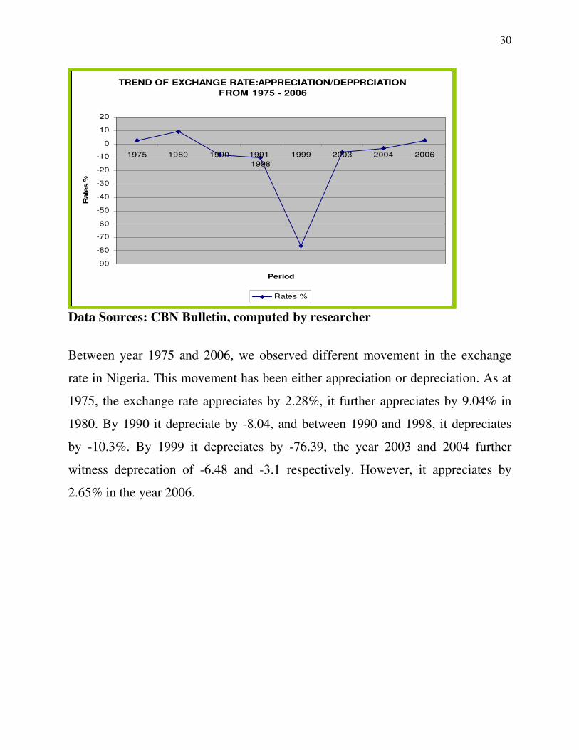
Data Sources: CBN Bulletin, computed by researcher
Between year 1975 and 2006, we observed different movement in the exchange
rate in Nigeria. This movement has been either appreciation or depreciation. As at
1975, the exchange rate appreciates by 2.28%, it further appreciates by 9.04% in
1980. By 1990 it depreciate by -8.04, and between 1990 and 1998, it depreciates
by -10.3%. By 1999 it depreciates by -76.39, the year 2003 and 2004 further
witness deprecation of -6.48 and -3.1 respectively. However, it appreciates by
2.65% in the year 2006.

31
CHAPTER THREE
METHODOLOGY
3.1 The model
The study will follow a simple linear specification of the multivariate time series
function using the partial adjustment approach to estimating given parameters of a
model. In so doing, Autoregressive Distributed Lag Model (ADLM) shall be used.
This is because past value of exchange is likely to determine the present value and
also the relationship between exchange rate and macroeconomic fundamentals that
determine it are likely to be dynamic in nature. That is, these determinants may
transmit beyond the present period. Consequently, The ADLM model will allow
the joint estimation of relationships between exchange rate and the
macroeconomics variables. Furthermore, there may be the need for us to transform
the model into an Autoregressive Distributed Lag Error Correction (ADL-ECM)
Model if at any point in time; there is evidence of co-integration among the
variables. The ECM will help to capture both the long run and the short run
dynamics of exchange rate and macroeconomics variables (See Engle and Granger,
1987).
3.2 Model Specification
Following the argument of Williamson, (1994) that a country’s optimal real
exchange rate is determined by its macroeconomic fundamentals (i.e. some key
macroeconomic variables) and that the long-run value of the real exchange rate is
determined by suitable (permanent) values of these fundamentals, we formulate the
determinant of real exchange rate in Nigeria as follows;
( ), , , ...................(1)RER F GDPR INTR INF TOP=
where
RER = Real Exchange Rate
32
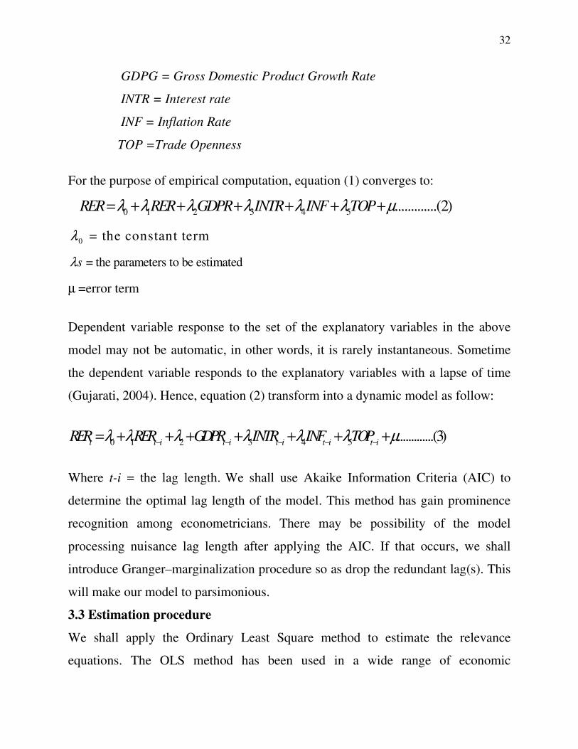
GDPG = Gross Domestic Product Growth Rate
INTR = Interest rate
INF = Inflation Rate
TOP =Trade Openness
For the purpose of empirical computation, equation (1) converges to:
0 1 2 3 4 5 .............(2)RER RER GDPR INTR INF TOPλ λ λ λ λ λ µ= + + + + + +
0 = the constant termλ = the parameters to be estimatedsλ
µ =error term
Dependent variable response to the set of the explanatory variables in the above
model may not be automatic, in other words, it is rarely instantaneous. Sometime
the dependent variable responds to the explanatory variables with a lapse of time
(Gujarati, 2004). Hence, equation (2) transform into a dynamic model as follow:
0 1 2 3 4 5 .............(3)t t i t i t i t i t iRER RER GDPR INTR INF TOPλ λ λ λ λ λ µ− − − − −= + + + + + + +
Where t-i = the lag length. We shall use Akaike Information Criteria (AIC) to
determine the optimal lag length of the model. This method has gain prominence
recognition among econometricians. There may be possibility of the model
processing nuisance lag length after applying the AIC. If that occurs, we shall
introduce Granger–marginalization procedure so as drop the redundant lag(s). This
will make our model to parsimonious.
3.3 Estimation procedure
We shall apply the Ordinary Least Square method to estimate the relevance
equations. The OLS method has been used in a wide range of economic

33
relationship with satisfactory result. The method employs a sound statistical
technique appropriate for empirical problems; and it has become so standard that
its estimates are presented as a point of reference even when result from other
estimation technique are used. More so, the reliability of this method lies on its
desirability properties which are efficiency, consistency and unbiased. This implies
that its error term has a minimum and equal variance. The conditional mean value
is zero and normally distributed (Gujarat, 2004).
3.4 Unit Root Test
Conventionally, the universal assumption in building and testing economic models
that underlies variables are stationary, but is unfortunately not generally true.
Before estimating our model in equation (3), we shall check for the time series
properties of the data. This is necessary because time series econometricians such
as Granger and Newbold, (1974); Eagle and Granger, (1987), Dickey and Fuller,
(1981); Enders, (1995); Pindyck and Rubinfeld, (1998),among others, observed
that results emanating from most macroeconomic variables are likely to be
“Spurious” if the time series properties of such series are not examined. Hence, the
time series properties of the data would be examined using Augmented Dickey
Fuller (ADF) test and the Engle-Granger co-integration procedure.
The testing procedure for the ADF is as follows:
0 1 1 1 ... .........(4)t t t p t p tRER t RER RER RER Uλ β γ δ δ− − −∆ = + + ∆ + ∆ + + ∆ +
where
�0 is a constant, �t is the coefficient on a time trend and p is lag order of the
autoregressive process and � is difference operator. The unit root test is then
carried out under the null hypothesis � = 0 against the alternative hypothesis of � <
0. If the test statistic is greater (in absolute value) than the critical value let say at

34
5% or 1% level of significance, then the null hypothesis of � = 0 is rejected and no
unit root is present.
From the above discussion, our model in equation (3) becomes;
0 1 2 3 4 5 .............(5)t t i t i t i t i t iRER RER GDPR INTR INF TOPλ λ λ λ λ λ µ− − − − −∆ = + ∆ + ∆ + ∆ + ∆ + ∆ + Where, � is the difference operator. 3.5 Co-integration Test
If RER and the explanatory variables are linked by some long-run relationship,
from which they can deviate in the short run but must return to in the long run, the
residuals obtain from their linear combination will be stationary. If the variables
diverge without bound (i.e. non-stationary residuals) we must assume no
equilibrium relationship exists. In other words, if RER and any of the explanatory
variable(s) are both integrated of order d (i.e. I(d)), then, in general, any linear
combination of the RER and any of the explanatory variables will also be I(d); that
is, the residuals obtained from regressing RER on the explanatory variable(s) are
I(d). Should the residual is stationary it implies there is evidence of long run
relationship among the variables. Hence our model in equation (5) becomes;
0 1 2 50 0 0
... ........(6)n n n
t t t t t t i Iti i i
REX REX GDPG TOPλ λ λ λ β µ µ−= = =
∆ = + ∆ + ∆ + + ∆ + +∑ ∑ ∑
Where;
11 −t
uβ = Error Correction Representation
1
β = Coefficient measuring the degree of error corrected
Hence, the model in equation (6) is the Autoregressive Distributed Lag Error
Correction Model (ADLECM) we hope to estimate if there is evidence co-
integration among the variables. On the contrary, if there is no co integration

35
among the variables we shall estimate the Autoregressive Distributed Lag Model
specified in equation (5). 3.6 Techniques of Results Evaluation
We shall use three basic criteria to evaluate the results obtain from the model;
economic (a priori expectations), statistical and econometric criteria. The economic
criteria will inform us if the signs of the variables coefficient conform to economic
theory. While the Statistical criteria shall focus on testing the significance of the
variables using T-test, and F-statistic will be used to assess the joint significance of
the overall regression in order to see whether the model is well specified. In the
same, the econometric criterion would involve such tests as autocorrelation and
multicollinear. The autocorrelation will help to check for the existence of serial
correlation among the variables, while the multicollinear test would help to check
if the variables are collinear.
3.7 Model Justification
There are varieties of model available to econometricians/researchers when
modeling. However the choice of a particular model is base on reliability,
effectiveness and adequacy of the model. Thus among the numerous rival models,
we opted for Autoregressive Distributed Lag Error Correction model (ADLM-
ECM). The choice of this model is informed by the fact that, apart from the
efficiency of the ADLM, it will also help to draw inferences about dynamic
behavior of the variables since it has been established that it take lapse of time for
the dependent variables to response to the explanatory variables when modeling.
Also, the ECM will be most appropriate and efficient model that can capture the
long run behavioral pattern of variables under co-integration situation (See Enders,

36
1995). Lastly, the model will take care of the problem of the so-called “spurious”
regression associated with non-stationary data.
3.8 Data Sources
The data for this study are secondary in nature. They shall be obtained from the
Central Bank Nigeria Statistical Bulletin 2006 publication
3.9 Econometric software
We shall use PC-GIVE software, for the analysis after the data must have been
loaded into Microsoft Excel worksheet and then imported into the PC-GIVE.
37
CHAPTER FOUR
PRESENTATION AND INTERPRETATION OF RESULT
4.1 Overview
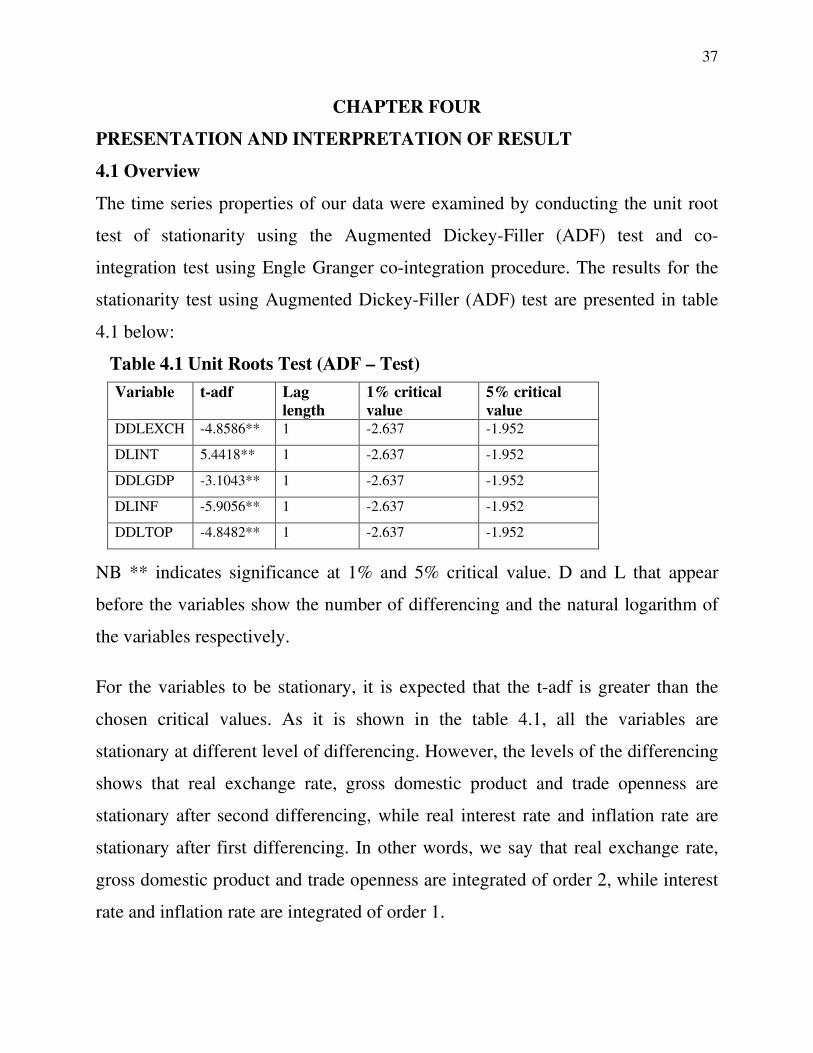
The time series properties of our data were examined by conducting the unit root
test of stationarity using the Augmented Dickey-Filler (ADF) test and co-
integration test using Engle Granger co-integration procedure. The results for the
stationarity test using Augmented Dickey-Filler (ADF) test are presented in table
4.1 below:
Table 4.1 Unit Roots Test (ADF – Test) Variable t-adf Lag
length 1% critical value
5% critical value
DDLEXCH -4.8586** 1 -2.637 -1.952
DLINT 5.4418** 1 -2.637 -1.952
DDLGDP -3.1043** 1 -2.637 -1.952
DLINF -5.9056** 1 -2.637 -1.952
DDLTOP -4.8482** 1 -2.637 -1.952
NB ** indicates significance at 1% and 5% critical value. D and L that appear
before the variables show the number of differencing and the natural logarithm of
the variables respectively.
For the variables to be stationary, it is expected that the t-adf is greater than the
chosen critical values. As it is shown in the table 4.1, all the variables are
stationary at different level of differencing. However, the levels of the differencing
shows that real exchange rate, gross domestic product and trade openness are
stationary after second differencing, while real interest rate and inflation rate are
stationary after first differencing. In other words, we say that real exchange rate,
gross domestic product and trade openness are integrated of order 2, while interest
rate and inflation rate are integrated of order 1.

38
4.2 Co integration test
From the unit root test in table 4.1, we noticed that real exchange rate which is the
dependent variable in the specified equations have the same order of integration
with gross domestic product and trade openness which are independent variables,
we then estimated their linear combination without the constant term and obtain
their residual which was tested for unit root test of stationary using Augmented
Dickey Fuller. The outcome of the test is given below: Table 4.2 co integration result
t-adf lag 5% critical value
1% critical value
Residual -3.0838** 2 -1.951 -2.632
Residual -2.8096** 1 -1.951 -2.632
Residual -3.1688** 0 -1.951 -2.632
The result shows the existence of co-integration among the variables because the
residual obtained from the linear combination of none stationary series is stationary
at both 5% and 1% critical values. Hence there is necessity to estimate an Error
Correction Model (ECM) that is the model in equation number (6).
4.3 Presentation of Dynamic ECM modeling of REXCH result
Table 4.3 Result Summary
Variables Coefficient Std.Error T-value T-prob Part YR ˆ
CONSTANT 0.049238 0.054465 0.904 0.3754 0.0343
DDLEXCH_1 -0.42343 0.16501 -2.566 0.0173 0.2226
DLINT 0.35261 0.27102 1.301 0.2061 0.0686
DLINT_1 0.22703 0.26289 0.864 0.3967 0.0314
DDLGDP 0.079066 0.2148 1.276 0.2148 0.0661
DDLGDP_1 0.38623 0.27671 1.396 0.1761 0.0781
DLINF -0.10849 0.070760 -1.533 0.1389 0.0927

39
DLINF_1 -0.15561 0.078079 -1.993 0.0583 0.1473
DDLTOP -0.0072796 0.13445 -0.054 0.9573 0.0001
DDLTOP_1 -0.37950 0.17008 -2.231 0.0357 0.1779
ECM_1 -0.012684 0.0041802 -3.034 0.0059 0.2859
R2 =0.660298, DW = 1.86, F-Stat (10, 23) = 4.4706
4.4 Interpretation of Result
From the result, the constant term is positive, even though it does not have any
economic meaning, it meet our a priori expectation. That is if other variable that
contribute to real exchange rate is zero, there are other variables that can contribute
in a positive or negative way to real exchange rate
The lag value of real exchange rate has a negative and significant relationship with
real exchange rate. The result shows that a 10% increase in the past value of real
exchange rate leads to 42% decrease in real exchange rate. The t-value of -2.566
which is greater than absolute 2 using a 2-t Rule of Thumb is statistically
significant suggest that the past one year value of real exchange rate is a major
determinant of real exchange rate in Nigeria.
The current and immediate past year value of real interest has a direct relationship
with real exchange rate. A 10% increase in real interest in the current and previous
one year leads to 35% and 0.22% increase in real exchange rate respectively. The
positive sign display by real interest rate meet economic apriori expectation since
interest rate differentials will affect the equilibrium exchange rate. A rise in
Nigeria interest rates relative to other countries rates all things being equal, will
cause investors to switch from their currency to Naira-denominated securities to
take advantage of the higher Naira rates. The net result will be depreciation of the
Naira in the absence of government intervention. However, the result indicates that

40
real interest is not a major determinant of real exchange rate in Nigeria as shown
by its t-values of 1.301 and 0.864 which are statistically insignificant.
Similarly, gross domestic product growth rate has a direct and insignificant
relationship with real exchange rate both in the current and previous year. From the
regression result, a 10% increase in gross domestic product growth rate causes real
exchange rate to increase by 7.9% and 38% in the current year and immediate past
year respectively. The positive signs display by real gross domestic product growth
rate meet economic a priori expectation. This is because a nation with strong
economic growth will attract investment capital seeking to acquire domestic assets.
The demand for domestic assets in turn will results in an increased demand for the
domestic currency and a stronger currency, other things being equal. Empirical
evidence supports the hypothesis that economic growth should lead to a stronger
currency. Conversely, nations with poor growth prospects will see an exodus of
capital and weaker currencies. However, the result shows that gross domestic
product growth rate is not statistically significant in the analysis showing that it is
not a major determinant of real exchange rate in Nigeria.
Inflation rate displays a negative insignificant relationship with real exchange rate
both in the current year and past one year. From the regression result, a 10%
increase in inflation rate causes 10% and 15% decrease in real exchange rate in the
current and immediate past year respectively. Notwithstanding, inflation rate is not
a significant factor that determine country real exchange rate.
Surprisingly, while trade openness both at the current and past one year value has a
negative relationship with real exchange rate, the current year value is insignificant
in determine real exchange rate, while the past one year value appeared to be one
of the major determinant of real exchange in Nigeria. According to the regression

41
result, a 10% increase in trade openness in the current and previous year leads to
0.72% and 37% decrease in real exchange rate respectively. The fact that trade
openness is statistically significant in determine real exchange rate suggests the
important of external factors in the determination of real exchange rate in Nigeria
and the fact that trade openness is expected to transmits its impact through
unexpected changes in the exchange rate.
4.5 coefficient of determination R2
In the error correction model, we expect a lower R2, given that the dependent
variable is differenced. Given the parsimonious specification, the size of the R2 is
impressive. The R2 is 0.660298 shows that the explanatory variables (lag of real
exchange rate, real interest rate, inflation rate, and gross domestic product growth
rate) explained 66% of the total variation in real exchange rate.
4.6 Test of Autocorrelation
The underlying assumption of autocorrelation is that the successive values of the
random Mi are temporally independent. The convectional Durbin Watson d
statistics is employed. Since DW which is 1.86 is close 2 rather than zero, we
conclude that there is autocorrelation.
4.7 F- test
We also conducted the f-test to check for model adequacy.
Hypothesis formulation
H0: the model is well specify
H1: there is misspecification of model
Decision Rule: If F-tabulated > F-calculated, we accept H0,
F (11, 21) =4.4706 and F- Table =2.65

42
Since the F-calculated of 4.4706 is greater than the F-tabulated of 2.65 at 5% level
of significance, we accept H0 and reject H1. Thus we concluded that the model is
good and well specified.
4.8 Test of Multicollinearity
We used the correlation matrix table in test for multicollinearity among the
variables. Gujarati, (2004) states that two explanatory variables is said to be
multicollinear if the pair –wise or zero – order correlation coefficient of the
variables is in excess of 0.8.
Table 4.4 Correlation Matrix
VARIABLE DDLEXCH DLINT DDLGDP DLINF DDLTOP DDLMS
DDLEXCH 1.000
DLINT 0.2705 1.000
DDLGDP 0.1191 0.2462 1.000
DLINF -0.01386 0.2462 0.2281 1.000
DDLTOP 0.2205 0.2764 -0.6084 -0.1868 1.000
DDLMS -0.2264 0.03066 0.05026 -0.06480 -0.005806 1.000
As the result in the table shows, that there is no multicollinearity among the
variables since none of the pair -wise correlation coefficient between any two
explanatory variables is above 0.8.

43
CHAPTER FIVE
SUMMARY, CONCLUSION AND POLICY RECOMMENDATION
5.1 Summary and Conclusion
This study examined the determinants of real exchange rate in the recent years in
Nigeria over the period of 1970 to 2006 using the Nigerian time series data.
Following literature, we identified the potential determinants of real exchange rate
as lag of real exchange rate, real interest rate, inflation rate, trade openness and real
gross domestic product. We started the modeling by examined the time series
characteristics of the data. Specifically, we conducted the stationarity test using
Augmented Dickey-Fuller (ADF) unit roots test and co-integration test using
Engle-Granger procedure. The variables were stationarized at different integration
level.
The accompanying co-integration test revealed there is an evidence of co-
integration between two explanatory variables (gross domestic product growth
rate, trade openness and the dependent variable real exchange rate. Arising from
this scenario; we employed the Auto-regressive Distributed Lag Model (ARDL-
ECM) specified in equation number (6). Initially, using the Akaike information
criteria (AIC), we adopted 4-period lag lengths. However, applying Granger
marginalization procedure we are able to drop 3-period lag lengths as we perceived
they are redundant in the model. Hence the parsimonious model was achieved
using one period lag length. The overall outcome of the estimations is adjured
satisfactory by the fact that the outcome of the results meet
The empirical result shows on the first hypothesis that the lag value of real
exchange rate has a negative and significant relationship with real exchange rate.
The result suggests that one year past value real exchange rate is a major
44
determinant of real exchange rate in Nigeria. The current and past value of real
interest has a positive relationship with real exchange rate, but it is however not
statistically significant to determine real exchange rate in Nigeria. Similarly, gross
domestic product growth rate is not a major determinant of real exchange rate in
Nigeria. Inflation rate investment displays a negative relationship with real
exchange rate both in the current and past one year. Notwithstanding, inflation rate
is not a significant factor determine country real exchange rate. Lastly, while trade
openness both at the current and past one year value has a positive relationship
with real exchange rate, the current year value is insignificant to determine real
exchange rate, while the past one year value appeared to be one of the major
determinant of real exchange in Nigeria.
On the second hypothesis, the result obtained indicates that there is evidence of
long run relationship between real exchange rate and two explanatory variables
(gross domestic product growth rate and trade openness).
5.2 Policy Recommendation
The findings above have some implication for dynamic monetary policy
formulations in Nigeria mostly in determine the real exchange rate in Nigeria.
Arising from this, we propose the following recommendations for the economy.
The lag of real exchange rate have a crucially effect on expectations of future
exchange rate changes, this will aid the forecasts of future economic conditions.
Therefore, sound policies and management should consolidate on this lag impact
so as to better the economy.
The study shows that real exchange rate responds positively to real interest rates.
Monetary policy is crucial here. There is need for the monetary authority to pursue

45
interest rate stability as swings in interest rate will post a serious treat to
maintaining stability in real exchange rate.
The pursuance of a stable exchange rate regime that results in a balance of
payments position that is viable and sustainable is one of the ultimate goals of
monetary policy. The pursuits of this objective and the extent to which they are
met have important implications for investment decisions, and, indeed,
international capital flows into Nigeria, especially in increasingly globalised
financial markets. Hence, we suggest that the exchange rate has to be competitive,
in order to attract foreign investors in Nigeria. That is, the exchange rate should,
and indeed, must reflect market realities to promote efficiency in resource
allocation and productivity growth. Therefore, the goal of CBN should be to
pursue monetary policy that is consistent with the maintenance of a realistic and
stable exchange rate regime, vis-à-vis those of our trading partners.
Findings from this study shows that trade openness is one of the major determinant
of real exchange rate in Nigeria. Depreciation in exchange rate will make Nigeria’s
export cheaper relative to imports, this will increase the country’s export receipts
and in turn improve the position of the foreign reserve. The exchange rate should
not be allowed to appreciate too much, since it may reduce the foreign reserve of
the country as well as to be able to import at lower cost.
Equally worthy to note is the fact that there has been a remarkable improvement in
the annual average depreciation rate which implies a stronger currency for the
country. Government should try to encourage monetary policies so as to maintain
the strength of the naira.

46
Government should pursue strategies that are designed to neutralize the effects of
such practices as round tripping, over-invoicing and under-invoicing which have
characterized the activities of the banking sectors in the recent years.
Lastly, foreign exchange control policies should be adopted in order to help in
determination of appropriate exchange rate value. This will go a long way of
strength the naira.
5.3 Conclusion
A major gain from Nigeria’s adoption of structural adjustment programme was the
liberalization of the foreign exchange market, in which the determination of the
exchange rate of the national currency (Naira) has largely been dictated by market
forces. This has helped to enhance efficiency in the allocation and utilization of
foreign exchange resources. Over the years, various types of market mechanisms
have been adopted, with Dutch Auction System (DAS) being the latest. The
introduction of DAS has been a giant step in promoting increased flexibility in the
management of the naira exchange rate. Under the DAS, satisfactory progress has
been made to make naira exchange rate to be truly market-determined.
However, there are some considerations for adopting a particular exchange rate
regime. If the market behaves in an efficient and rational manner, then free floating
is the proper policy to follow. If the market occasionally produces irrational and
inefficient outcomes (market failure), then managed floating will be an appropriate
policy. The actual exchange rate regime chosen by the authority will have
consequences in the economy. Most countries will not follow a prescribed
exchange rate regime due to different circumstances facing the economy for every
external shock. For instance, developing economies like Nigeria are subject to
external shock of investor sentiment and market participants’ perception of risk.
47
Also, business cycle, monetary policy, and fiscal policy of developed countries
have impact on the economies of developing countries and their exchange rates.
The choice between floating and hard peg depends on the inflationary history of
the economy and its own characteristics. Finding the exchange rate that serves
many economic objectives is not an easy task. The appropriate regime at any given
time for a given economy should be based on the structural characteristics and the
flexibility of that economy
48
REFERENCES
Agu, C. (2002) “Real Exchange Rate Distortions and External Balance Position of Nigeria: Issues and Policy Options. Journal of African Finance and Economic Development 2002, V 5 2, pp 143-174.
Agnes and Coeure (2001) “The survival of Intermediate Exchange Rate Regimes”
Journal of Political Economy, 204-566. Akinmoladun, C. E. (1990) Foreign Exchange and International trade in Nigeria,
Lagos, Gene Publications. Amartya Lahiri, Rajesh Singh & Carlos Vegh (2004) ‘Segmented Asset Markets
and Optimal Exchange Rate Regimes’. Federal Reserve Bank of New York, Iowa State University and UCLA and NBER
Barnett W. A. and Kwag C. H. (2005). “Exchange Rate Determination from
Monetary Fundamentals: an Aggregation Theoretic Approach”, Department of Economics
University of Kansas Lawrence, KS 66045-7585 and India Study Institute POSCO Research Institute POSRI Building 147 Samsungdong Kangnamgu Seoul 135-878, Korea
Batini N. and Levine P. (2006). “Optimal Exchange Rate Stabilization in a
Dollarized Economy with Inflation Targets” International Monetary Fund and University of Surrey Joseph Pearlman London Metropolitan University.
Benigno G. and Benigno P. (2004). “Exchange Rate Determination under Interest
Rate Rules” New York University. Bruno C. And Pugh G. (2006). “The Effects Of Exchange Rate Variability On
International Trade: A Meta Regression Analysis” University Of Split, Faculty Of Economics, Working Paper
CBN (1998) “Nigeria’s Exchange Rate Policy” A CBN Research Department
Series. Chuka, S. R. (1990) ''The Exchange Rate and Exchange Controls as Instruments of
Economic Policy: The Experience of Malawi'', unpublished paper presented

49
at a seminar on ''Experience with Instruments of Economic Policy'', in Addis Ababa, Ethiopia
Corden, W. X. (2001) “Corden Says Developing Countries’ Choices Vary
According to Specific Economic Circumstances”. IMF Survey, Vol. 30, No. 3, February.
Deverux M. and Engel C. (1988) ‘Fixed floating exchange rates: how price setting
affects the optimal choice of exchange-rate regime,’ National Bureau of Economic Research (NBER) working paper 6867, www.nber.org/papers/w6867
Devereux, M. B. And Engel C. [2000], “Monetary Policy In The Open Economy
Revised: Price Setting And Exchange Rate Flexibility”,NBER Working Paper No. 765
Dickey, D.A. and Fuller W. A. (1981), Likelihood Ratio Statistics for
Autoregressive Time Series with a unit Root. Econometrical. Dornbusch, R. (1976) ‘Expectation and exchange rate dynamic’, Journal of
Political Economy, reprinted in Dornbusch [1988 ed.] ‘Open Economy Macroeconomics’ NY: Basic Books Publisher.
Dornbusch, R. (1988) ‘Purchasing Power Parity’, in the ‘New Palgrave: A
Dictionary of Economics’, NY: Stockton Press. Dornbusch, R. (2004) ‘Expectation and exchange rate dynamic’, Journal of
Political Economy, reprinted in Dornbusch [1988 ed.] ‘Open Economy Macroeconomics’ NY: Basic Books Publisher.
Dornbusch R, Fischer S and Startz (2004) “Macroeconomic” New York Worth
Publisher. El-Mefleh M. (2004) “The Elusiveness Of An Optimal Exchange Rate” American
Association of Behavioral Social Science Online Journal Enders W. (1995), Applied Econometrics Time Series. John Willey and sons Inc. Engel C. (2000). “Exchange Rate Policy” National Bureau of Economic Research
Working Paper.

50
Engle, R. F. and Granger, C. W. (1987), Co-integration and Error Correction:
Representation, Estimation and Testing. Econometrical. Faia E. (2005) Optimal Choice of Exchange Rate Regimes with Labour Market
Frictions, University of Rome at Tor Vergata and Ente Einaudi Institute for Economics and Finance
Frankel, Jeffrey A. (1978). On the Mark: A Theory of Floating Exchange Rates Based on Real Interest Rate Differentials. American Economic Review 69: 610–22
Friedman, M. (1953). The case for flexible exchange rates, in Essays in Positive Economics (Chicago: University of Chicago Press), 157-203
. Granger, C. and Newbold, (1974), Spurious Regression in Econometrics. Journal
of Econometrics 2. Gujarati, D. (2004), Basic Econometrics, Tata McGraw-Hill Publishing Limited
New Delhi. Hoontrakul P. (1999). Exchange Rate Theory: A Review” Sasin-GIBA,
Chulalongkorn University, Thailand. Hooper, P., and J. Morton (1982), “Fluctuations in the Dollar: A Model of
Nominal and Real Exchange Rate Determination,” Journal of International Money and Finance
Jhingan M. L. (2005). International Economics,5th Edition, Vrinda Publications (P)
Limited Delhi. Jimoh, S. O. (2006). “Traditional Theory of Real Exchange Rate and Options”
Unpublished Thesis submitted to the Department of Banking and Finance, Enugu State Science and Technology.
Kandil M. (2004). “Exchange Rate Fluctuations and Economic Activity in Developing Countries: Theory and Evidence” Journal of Economic Development.

51
Kildegaard, A. (2005). “Fundamentals of Real Exchange Rate Determination: What Role in the Peso Crisis?” University of Minnesota Morris, Morris, MN 56267, USA. E-mail: [email protected]. Phone: (320)589-6190. Fax: (320)589
Krueger, A. O. (1983). Exchange Rate Determination, Cambridge Press
Leo, V. (2OO6). “ Choosing an Exchange Regime: The challenges for Countries” IMF, Washington DC.
MacDonald, Ronald and Mark P. Taylor (1994), “The Monetary Model of the
Exchange Rate:Long-run Relationships, Short-run Dynamics, and How to Beat a Random Walk,” Journal of International Money and Finance.
Maciejewski, E. B.(1983) Real Effective Exchange Rate Indices” IMF Staff
Papers 30(3): September 491-525. Mankiw M.G. (1997) “Macroeconomics” New York Worth Publisher Meese, R. and K. Rogoff (1990): Empirical Exchange Rate Models of the
Seventies: Do they Fit Out of sample? Journal of International economics 14, 3-24.
Mundell, Robert A., (1963), Capital mobility and stabilization policy under fixed
and flexible exchange rates, Canadian Journal of Economics and Political Science 29, 475-485.
NEEDS (2004) National Economic Empowerment Strategy. Abuja.National
Planning Commission. Obadan, M. I. (1992) “Overview of Nigeria’s Exchange Rate Policy and
Management since the Structural Adjustment Programme” CBN Economic and Financial Review, Vol.31 No. 8, June.
Obadan, M. I. (2003). “Exchange Rate Mechanism under the West African
Monetary Zone “(Wamz) Mimeograph.
Obioma, N. E. (2000). Elements of International Economics Lagos: Impresses Publishers.

52
Obstfeld, Maurice and Kenneth Rogoff, (1995), Exchange rate dynamics redux, Journal of Political Economy 103, 624-660.
Ojamenaye, C. (1991) “Naira Exchange Rate Policy Since 1986” Seminar Paper on
The Naira Exchange Rate: Problems and Prospects, Lagos. Ojo, M. 0. (1991). “An Overview of the Central Bank of Nigeria Decree No. 24” CBN BULLION, Vol.15, No.4, October December, 1991. CBN, Lagos. Ojo, M.O. (1998). “Exchange Rates Developments in Nigeria: A Historical
Perspective”. Being Text of a paper delivered at a Seminar on “Exchange Rate Determination and Arithmetic” by Unilag Consult.
Pindyck, R. and Rubinfeld D. (1998), Econometric Models and Economic
Forecast. Singapore McGrw-Hill in Ed. 4. Sanusi, J.O. (1988) Deregulating the Nigerian economy: Achievements and
prospects, Economic and Financial Review. The Central Bank of Nigeria, vol. 26, no. 4: 32-40.
Sanusi J.O (2004) Exchange Rate Mechanism: The Current Nigerian Experience,
A Paper Presented At The Nigerian British Chamber Of Commerce Shehu, A. and Aliyu M. (2006). “Naira Exchange Rate and Policy Management”
Unpublished Thesis submitted to the department of Economics, University of Benin.
Sodersten, B. C. (1997), International Economics 2nd Edition (Macmillan)
Taylor, M.P. (1995): The Economics of Exchange Rates. Journal of Economic
Literature, Vol. XXXIII, 13-47
Williamson, J. (1994). "Advice on the choice of an exchange rate policy". In E.M. Classen, ed. Exchange Rate Policies in Developing and Post Socialist Countries. San Francisco, California: ICEG Publications.
World Bank (2000) Nigeria Financial Sector Review, financial Sector Unit
Economic Management and Social Policy Department Africa Region.

53
APPENDIX YEAR EXCH INT GDPGR INF TOP
1970 0.7143 7 10 13.8 28107
1971 0.6955 7 18.39 16 36876
1972 0.6579 7 7.29 3.2 38549
1973 0.6579 7 9.52 5.4 45092
1974 0.6299 7 5.94 13.4 77165
1975 0.6159 6 0.18 33.9 55212
1976 0.6265 6 10.77 21.2 59731
1977 0.6466 6 -6.7 15.4 69201
1978 0.606 7 -6.72 16.6 49579
1979 0.5957 7.5 2.63 11.8 66595
1980 0.5464 7.5 2.9 9.9 79403
1981 0.61 7.75 -8.4 20.6 56782
1982 0.6729 10.25 -0.6 7.7 45621
1983 0.7241 10 -4.9 23.2 32105
1984 0.7649 12.5 5.8 39.6 34113
1985 0.8938 9.25 10.5 5.5 42253
1986 2.0206 10.5 -1.8 5.4 33262
1987 4.0179 17.5 -4 10.2 70563
1988 4.5367 16.5 9.4 34.5 60593
1989 7.3916 26.8 8.5 50.5 124653
1990 8.0378 25.5 13.8 7.4 214793
1991 9.9095 20.01 -2.6 12.7 131554
1992 17.298 28.8 2 44.8 120794
1993 22.051 36.09 1.5 57.2 111668
1994 21.886 21 -0.6 57 82026
1995 21.886 20.18 2.3 72.8 122400
1996 21.886 19.74 6.6 29.3 110899
1997 21.886 13.54 3.2 8.5 147505
1998 21.886 18.29 0.3 10 114850
1999 92.693 21.32 1.5 6.6 195323
2000 102.11 17.98 5.4 6.9 242676
2001 111.94 18.29 3.1 18 239014
2002 120.97 24.4 1.5 13.7 246820
2003 129.36 20.48 10.7 14 278593
2004 133.5 19.15 6 15 292396
2005 131.66 17.85 7.2 17.8 310731
2006 128.33 18.2 5.6 8.3 5752884 Source: Extract from CBN Statistical bulletin 2006 publication Note: Gross domestic product growth rate and trade openness was computed by researcher

54
---- PcGive 8.00, copy for meuller ---- ---- session started at 3:11:11 on 24th February 2010 ---- LEXCH = log(EXCH); DLEXCH = diff(LEXCH, 1); DDLEXCH = diff(DLEXCH, 1); LINT = log(INT); DLINT = diff(LINT, 1); DDLINT = diff(DLINT, 1); LGDP = log(GDP); DLGDP = diff(LGDP, 1); DDLGDP = diff(DLGDP, 1); LINF = log(INF); DLINF = diff(LINF, 1); DDLINF = diff(DLINF, 1); LTOP = log(TOP); DLTOP = diff(LTOP, 1); DDLTOP = diff(DLTOP, 1); Unit root tests 6 to 37 Critical values: 5%=-1.952 1%=-2.637 t-adf å lag t-lag t-prob LEXCH 0.80749 0.34250 2 0.40869 0.6858 LEXCH 1.0763 0.33771 1 1.2844 0.2088 LEXCH 1.8141 0.34123 0 DLEXCH -2.0545* 0.34203 2 -0.85687 0.3985 DLEXCH -2.7352** 0.34051 1 -0.80541 0.4269 DLEXCH -3.9453** 0.33858 0 DDLEXCH -4.8586** 0.36106 2 0.90080 0.3751 DDLEXCH -6.4918** 0.35992 1 1.8835 0.0694 DDLEXCH -8.8319** 0.37442 0 LINT 0.86171 0.22989 2 -1.5346 0.1357 LINT 0.57577 0.23502 1 -1.1362 0.2649 LINT 0.40195 0.23612 0 DLINT -2.6733** 0.21953 2 -1.9013 0.0672 DLINT -5.4418** 0.22890 1 1.4057 0.1701 DLINT -6.7403** 0.23247 0 DDLINT -5.3372** 0.24340 2 0.63636 0.5295 DDLINT -10.547** 0.24097 1 4.8773 0.0000 DDLINT -9.5586** 0.31742 0 LGDP 0.68172 1.2435 2 -0.10641 0.9160 LGDP 0.77432 1.2229 1 -1.2603 0.2173 LGDP -0.26236 1.2344 0 DLGDP -1.3562 1.2124 2 -1.4125 0.1684 DLGDP -1.9368 1.2324 1 -0.35873 0.7223 DLGDP -2.4438* 1.2150 0 DDLGDP -3.0645** 1.2040 2 1.5070 0.1426 DDLGDP -3.1043** 1.2293 1 1.9804 0.0569 DDLGDP -2.6451** 1.2859 0 LINF -0.44465 0.76298 2 -2.1856 0.0371 LINF -0.79750 0.80959 1 -0.15212 0.8801 LINF -0.84993 0.79673 0 DLINF -4.5209** 0.75964 2 0.67477 0.5052 DLINF -6.0900** 0.75271 1 2.3325 0.0266 DLINF -5.9056** 0.80482 0 DDLINF -5.6422** 0.96317 2 1.3236 0.1960

55
DDLINF -7.8940** 0.97517 1 3.1576 0.0036 DDLINF -7.7984** 1.1073 0 LTOP 1.3930 0.61138 2 -0.022043 0.9826 LTOP 1.4570 0.60111 1 -0.78018 0.4414 LTOP 1.3361 0.59730 0 DLTOP -1.1201 0.62440 2 -0.81431 0.4221 DLTOP -1.9691* 0.62089 1 -0.32969 0.7439 DLTOP -3.5329** 0.61190 0 DDLTOP -2.4672* 0.63734 2 -0.19668 0.8455 DDLTOP -4.8482** 0.62705 1 1.7931 0.0831 DDLTOP -7.1924** 0.64906 0 EQ( 1) Modelling EXCH by OLS The present sample is: 1 to 37 Variable Coefficient Std.Error t-value t-prob PartRý GDP -2.8593e-006 2.7964e-006 -1.022 0.3138 0.0298 TOP -1.6206e-005 7.1093e-006 -2.280 0.0290 0.1326 Rý = 0.943135 å = 14.0476 DW = 0.934 * Rý does NOT allow for the mean * RSS = 6709.423332 for 3 variables and 37 observations Residual added to database Residual = Residual values of equation 1 Unit root tests 4 to 37 Critical values: 5%=-1.951 1%=-2.632 t-adf å lag t-lag t-prob Residual -3.0838** 12.133 2 1.2485 0.2212 Residual -2.8096** 12.238 1 0.29457 0.7702 Residual -3.1688** 12.068 0 Solved Static Long Run equation EXCH = -2.859e-006 GDP -1.621e-005 TOP +7.912e-005 MS (SE) (2.796e-006) (7.109e-006) (1.347e-005) ECM added to database Analysis of lag structure Lag 0 1 2 3 4 5 ä EXCH -1 0 0 0 0 0 -1 Std.Err 0 0 0 0 0 0 0 GDP -2.86e-006 0 0 0 0 0-2.86e-006 Std.Err 2.8e-006 0 0 0 0 0 2.8e-006 TOP -1.62e-005 0 0 0 0 0-1.62e-005 Std.Err7.11e-006 0 0 0 0 07.11e-006 MS 7.91e-005 0 0 0 0 07.91e-005 Std.Err1.35e-005 0 0 0 0 01.35e-005

56
Tests on the significance of each variable variable F(num,denom) Value Probability Unit Root t-test -1.0225 -2.2795 5.8756 EQ( 4) Modelling DDLEXCH by OLS The present sample is: 4 to 37 Variable Coefficient Std.Error t-value t-prob PartRý Constant 0.049238 0.054465 0.904 0.3754 0.0343 DDLEXCH_1 -0.42343 0.16501 -2.566 0.0173 0.2226 DLINT 0.35261 0.27102 1.301 0.2061 0.0686 DLINT_1 0.22703 0.26289 0.864 0.3967 0.0314 DDLGDP 0.079066 0.061986 1.276 0.2148 0.0661 DDLGDP_1 0.38623 0.27671 1.396 0.1761 0.0781 DLINF -0.10849 0.070760 -1.533 0.1389 0.0927 DLINF_1 -0.15561 0.078079 -1.993 0.0583 0.1473 DDLTOP -0.0072796 0.13445 -0.054 0.9573 0.0001 DDLTOP_1 -0.37950 0.17008 -2.231 0.0357 0.1779 ECM_1 -0.012684 0.0041802 -3.034 0.0059 0.2859 Rý = 0.660298 F(10, 23) = 4.4706 [0.0014] å = 0.280914 DW = 1.86 RSS = 1.814995449 for 11 variables and 34 observations Testing for ARCH from lags 1 to 1 Chiý(1) = 0.28783 [0.5916] and F-Form(1, 25) = 0.21997 [0.6431] ARCH Coefficients: Constant Lag 1 Coeff. 0.08077 -0.09339 Std.Err 0.03918 0.1991 RSS = 1.0879 å = 0.208605 Normality test for Residual The present sample is: 4 to 37 Sample Size 34 Mean -0.000000 Std.Devn. 0.267782 Skewness 1.779350 Excess Kurtosis 4.307673 Minimum -0.428262 Maximum 1.006687 Normality Chiý(2)= 15.788 [0.0004] ** Testing for Heteroscedastic errors Chiý(12) = 13.609 [0.3264] and F-Form(12, 14) = 0.77865 [0.6645] V01=DLINT V02=DDLGDP V03=DLINF V04=DDLTOP V05=ECM_1 V06=DDLEXCH_1 Heteroscedasticity Coefficients: Constant V01 V02 V03 V04 V05 Coeff. 0.03087 0.1469 0.3368 -0.08211 -0.05661 -0.006918

57
t-value 0.5289 0.7161 1.261 -1.164 -0.4577 -0.9284 V06 V01ý V02ý V03ý V04ý V05ý Coeff. -0.005469 -0.2389 0.0006136 -0.001557 0.2319 0.0004271 t-value -0.03645 -0.4114 0.01246 -0.03136 1.56 1.619 V06ý Coeff. -0.2909 t-value -1.184 RSS = 0.661346 å = 0.217345 Normality test for Residual The present sample is: 4 to 37 Sample Size 34 Mean -0.000000 Std.Devn. 0.267782 Skewness 1.779350 Excess Kurtosis 4.307673 Minimum -0.428262 Maximum 1.006687 Normality Chiý(2)= 15.788 [0.0004] ** Testing for Heteroscedastic errors Chiý(12) = 13.609 [0.3264] and F-Form(12, 14) = 0.77865 [0.6645] V01=DLINT V02=DDLGDP V03=DLINF V04=DDLTOP V05=ECM_1 V06=DDLEXCH_1 Heteroscedasticity Coefficients: Constant V01 V02 V03 V04 V05 Coeff. 0.03087 0.1469 0.3368 -0.08211 -0.05661 -0.006918 t-value 0.5289 0.7161 1.261 -1.164 -0.4577 -0.9284 V06 V01ý V02ý V03ý V04ý V05ý Coeff. -0.005469 -0.2389 0.0006136 -0.001557 0.2319 0.0004271 t-value -0.03645 -0.4114 0.01246 -0.03136 1.56 1.619 V06ý Coeff. -0.2909 t-value -1.184 RSS = 0.661346 å = 0.217345 Descriptive statistics The present sample is: 3 to 37 Means DDLEXCH DLINT DDLGDP DLINF DDLTOP 3.015e-005 0.02730 -0.1978 -0.01875 0.07563 Standard Deviations DDLEXCH DLINT DDLGDP DLINF DDLTOP 0.3964 0.2243 1.253 0.8369 0.6922

58
Correlation matrix DDLEXCH DLINT DDLGDP DLINF DDLTOP DDLEXCH 1.000 DLINT 0.2705 1.000 DDLGDP 0.1191 0.05217 1.000 DLINF -0.01386 0.2462 0.2281 1.000 DDLTOP 0.2205 0.2764 -0.6084 -0.1868 1.000


