The contribution of reservoirs to global land surface water 1
storage variations 2
3
Tian Zhoua, Bart Nijssena, Huilin Gaob, and Dennis P. Lettenmaiera,c* 4
5
aDepartment of Civil and Environmental Engineering, University of Washington, 6
Seattle, WA 98195 7
bZachry Department of Civil Engineering, Texas A&M University, College Station, 8
TX 77843 9
cnow at: Department of Geography, University of California, Los Angeles, CA 90095 10
11
Journal of Hydrometeorology 12
13
*Corresponding author: Dr. Dennis P. Lettenmaier 14
Corresponding author email: [email protected] 15
16

1
Abstract 17
Man-made reservoirs play a key role in the terrestrial water system. They alter water 18
fluxes at the land surface and impact surface water storage through water management 19
regulations for diverse purposes such as irrigation, municipal water supply, 20
hydropower generation, and flood control. Although most developed countries have 21
established sophisticated observing systems for many terms in the land surface water 22
cycle, long-term and consistent records of reservoir storage are much more limited and 23
not always shared. Furthermore, most land surface hydrological models do not 24
represent the effects of water management activities. Here we evaluate the contribution 25
of reservoirs to seasonal water storage variations using a large scale water management 26
model to simulate the effects of reservoir management at basin and continental scales. 27
The model was run from 1948 to 2010 at a spatial resolution of 0.25-degree latitude-28
longitude. A total of 166 of the largest reservoirs in the world with a total capacity of 29
about 3900 km3 (nearly 60% of the globally integrated reservoir capacity) were 30
simulated. The global reservoir storage time series reflects the massive expansion of 31
global reservoir capacity; over 30,000 reservoirs have been constructed during the past 32
half century, with a mean absolute inter-annual storage variation of 89 km3. Our results 33
indicate that the average reservoir-induced seasonal storage variation is nearly 700 km3 34
or about 10% of the global reservoir storage. For some river basins, such as the Yellow, 35
seasonal reservoir storage variations can be as large as 72% of combined snow water 36

2
equivalent and soil moisture storage. 37

3
1. Introduction 38
Freshwater is a key limiting resource for human development. Nearly 70% of global 39
freshwater is stored with relatively long retention periods in ice caps, glaciers, 40
permanent snow, and groundwater (USGS, 2014). Freshwater stored with much shorter 41
retention times in rivers, lakes, seasonal snow, and soil moisture is the main contributor 42
to storage variability in large-scale water budgets at seasonal and inter-annual scales 43
(Kinter and Shukla 1990), and is the source of most of the water used by humans. 44
Water management activities, such as irrigation and municipal water supply, 45
hydropower generation, and flood control, substantially alter freshwater fluxes at the 46
land surface and impact surface water storage through redistribution in space and time. 47
Since the early 1900s, the global irrigated agricultural area has increased six-fold to 48
approximately 3.2 million km2 or about 2% of the global land area (according to FAO 49
Global Map of Irrigation Areas (GMIA) V5.0). Total irrigation water withdrawals are 50
now about 2700 km3/year, and account for about 70% of the consumptive water use 51
globally (Gordon et al. 2005). To accommodate this rapid increase in irrigation water 52
demand, more than 30,000 large dams have been built globally during the past half 53
century, which impound almost 7000 km3 water (Vörösmarty et al. 2003; Hanasaki, et al. 54
2006) or nearly 20% of annual river runoff (Vörösmarty et al. 1997, White, 2005). 55
Biemans et al. (2011) estimated that irrigation and reservoir regulation have decreased 56
global discharge by 2.1% or 930 km3/yr. In arid or semi-arid river basins, the impact of 57

4
irrigation and reservoir operation may be amplified. Wang et al. (2006) analyzed the 58
runoff from the Yellow River and suggested that anthropogenic activities have shifted 59
streamflow patterns and are responsible for a decrease in the discharge of the river by 60
nearly one-half over the past 50 years. 61
Water retained by global reservoirs has also created a “drag” on global sea level rise. 62
Chao et al. (2008) estimated that man-made reservoirs have caused an equivalent sea 63
level drop of about 30 mm (-0.55 mm/yr) over the past 50 years. Lettenmaier and Milly 64
(2009) gave a slightly smaller estimate of -0.5 mm/yr at the decadal timescale and 65
suggested that the rate has slowed in recent years due to a slowdown in new dam 66
construction. 67
In addition to their long-term impacts on the global and regional water cycles, 68
artificial impoundments also reshape variations in water storage and streamflow at 69
seasonal and inter-annual time scales. Hanasaki et al. (2006) simulated two-year 70
operations of 452 global reservoirs and found that the maximum change in monthly 71
runoff as a result of reservoir operation was as large as 34% in 18 basins around the 72
globe. Haddeland et al. (2006) modeled anthropogenic impacts on seasonal surface 73
water fluxes for a set of global river basins and suggested that monthly streamflow in 74
the western USA decreased by as much as 30% in June due to irrigation and reservoir 75
regulations, while monthly streamflow increased by as much as 30% in Arctic river 76
basins in Asia during the winter low flow period. Oki and Kanae (2006) argue that these 77

5
variations in streamflow can lead to water-related hazards such as droughts and floods 78
if societies fail to anticipate or monitor these changes in the hydrological cycle. 79
Furthermore, variations in reservoir storage have important implications for the carbon 80
cycle. For example, Tranvik et al. (2009) estimated that the CO2 emissions to the 81
atmosphere from global inland waters (including lakes, reservoirs, wetlands, and rivers) 82
are similar in magnitude to the CO2 uptake by the global oceans. 83
Several studies have attempted to quantify the seasonal and inter-annual variability 84
of water budget components on the global scale (Dirmeyer 1995; Coughlan and Avissar 85
1996; Biancamaria et al. 2010; Nijssen et al. 2001a; Gao et al. 2012; Pokhrel et al. 2012). 86
However, long-term and consistent records that focus on water management and 87
human impacts on the global water cycle are not widely available. Gauge networks that 88
record reservoir storage are less unified than stream gauge networks and their records 89
are not always shared. Large scale modeling tools that integrate hydrology and 90
anthropogenic impacts have mostly been used at annual time scales (e.g. Chao et al., 91
2008, Döll et al. 2009) and studies that investigate the contribution of human activities to 92
seasonal variations of global surface water storage are still lacking. Here we describe a 93
large scale water management model that estimates the effects of irrigation and 94
reservoir storage on global and continental water cycles by integrating the Variable 95
Infiltration Capacity (VIC) macro-scale hydrological model (Liang et al. 1994), a soil 96
moisture deficit-based irrigation scheme, and a basin-scale reservoir storage module. 97

6
The specific questions we address are: 1) what is the magnitude of seasonal variations in 98
reservoir storage at continental and global scales?; 2) how large are seasonal reservoir 99
storage variations compared with the seasonal variations in other land surface water 100
storage terms such as soil moisture and seasonal snow?; and 3) what is the magnitude 101
of inter-annual global reservoir storage variations over the period 1948-2010, during 102
which many dams were built? 103
2. Methods and data 104
We simulated irrigation water use and reservoir operations in 32 global river basins 105
(Figure 1) with a large-scale water management model to quantify the monthly 106
variations of reservoir storage within selected large river basins. Within these 32 basins 107
we explicitly simulated 166 large reservoirs with a total capacity of 3900 km3, which 108
accounts for nearly 60% of the global reservoir capacity. 109
2.1 Water management model 110
The water management model we used was developed by Haddeland et al. (2006) 111
and has two components, 1) a modified version of the VIC model (VIC-IRR), which 112
includes a soil-moisture-deficit-based irrigation scheme, and 2) a reservoir module for 113
dam release optimizations. 114
The VIC-IRR model integrates a standardized method of irrigation scheduling into 115
the regular VIC model (VIC version 4.0.6). Within each grid cell, the irrigated area is 116
7
represented as a fraction of the cell area, in the same manner that other land cover types 117
are represented (see Liang et al. 1994). The automatic irrigation scheduling is based on 118
the VIC-predicted soil moisture content for agricultural grid cells at every 119
computational step. Specifically, irrigation is represented in the model as additional 120
precipitation during the growing season that occurs when the soil moisture drops 121
below the wilting point. Water added to the irrigated grid cells is taken from local grid 122
cell runoff and upstream reservoirs. The additional precipitation continues on a daily 123
basis until soil moisture reaches field capacity or until reservoir storage is exhausted. 124
The reservoir module is coupled with a simple routing model (Lohmann et al. 1996; 125
Lohmann et al. 1998) to simulate dam releases for single or multiple purposes such as 126
irrigation, flood control, hydropower, and water supply. The Shuffled Complex 127
Evolution Metropolis algorithm (SCEM-UA) optimization algorithm (Vrugt et al. 2003) 128
is used to optimize monthly dam releases (Qout) given reservoir inflow (Qin), storage (S), 129
installed capacity (represented by hydrostatic head, h), downstream irrigation water 130
demand (Qd), as well as flood (maximum) discharge (Qf) and minimum dam release 131
(Qmin). The objective functions (listed in Table 1) for the optimization were determined 132
by the main uses of each dam as specified in the Global Reservoir and Dam (GRanD) 133
Database (Lehner et al. 2011). The optimization procedure was executed in series when 134
a dam had multiple purposes. Irrigation demands were given priority, followed by 135
flood control. Where applicable, any excess water was used to maximize hydropower 136
8
production. Readers are referred to Haddeland et al. (2006) for more details of the water 137
management model. 138
Simulation of the optimized dam releases (Qout) required three simulations with VIC-139
IRR. The first VIC-IRR simulation was a standard VIC run without irrigation water 140
extraction to determine evapotranspiration in the absence of irrigation (EVAPreg) as well 141
as Qf and Qmin. The latter two were determined after routing the flow to each reservoir 142
grid cell and calculating the mean of the annual maximum daily discharges (Qf) and the 143
seven-day consecutive low flow with a ten-year recurrence period (Qmin). The second 144
VIC-IRR simulation was used to determine evapotranspiration under the assumption 145
that water is freely available (EVAPfree) at all times. For each irrigated grid cell, the 146
monthly irrigation water demand was estimated as EVAPfree minus EVAPreg. The monthly 147
irrigation demands for each reservoir (Qd) were then estimated by summing the 148
demands from the downstream grid cells with a maximum distance of ten 0.25-degree 149
grid cells (~250km) from the river stem. If multiple reservoirs were located in separate 150
tributaries upstream of an irrigated area, demands from the downstream grid cells were 151
divided among the reservoirs based on the reservoir capacities. For reservoirs located 152
on the same river, irrigation demand for each reservoir was derived from the entire 153
downstream areas (including the shared area). During the third (and also the final) 154
model run, reservoirs located within the same river basin were simulated in sequence 155
from upstream to downstream. Aside from differences associated with travel time in the 156

9
channel system, the Qin to the downstream reservoir is essentially the sum of Qout from 157
the upstream reservoir and the streamflow from the contributing area between the two 158
reservoirs. The model was run for the 63-year period from 1948 through 2010 at a daily 159
time step at 0.25-degree latitude-longitude resolution for the basins in Figure 1. A 43-160
year model simulation (1948 to 1990) was used to produce the initial soil moisture and 161
snow state for the model runs over the entire period. Reservoir storage was set to 80% 162
of the capacity as the initial state. The vegetation and crop parameters were fixed over 163
the modeling period. Monthly reservoir storage time series were extracted starting from 164
1948 or from the year the dam was built through 2010. Other water budget terms 165
including the soil moisture in all three soil layers, surface runoff, baseflow, and snow 166
water equivalent (SWE) were exported and converted to mean monthly values (in the 167
case of fluxes such as surface runoff and baseflow) or end of month values (in the case 168
of states such as soil moisture storage or SWE). 169
2.2 Study basins 170
We focused on 32 river basins that we selected based on two criteria: 1) the river 171
basin should contain at least one reservoir with a capacity greater than 3 km3; and 2) the 172
area of the river basin should be larger than 600,000 km2. The storage threshold was 173
selected because the 300 largest reservoirs (capacity > 3km3) account for over 75% of the 174
total global reservoir storage capacity (Lehner et al. 2011). The area threshold was 175
selected because basins with an area greater than 600,000 km2 account for almost half of 176
10
the global land area excluding Greenland and Antarctica (GRDC 2013). Combining 177
these two selection criteria resulted in 25 basins. Seven additional basins were selected 178
(La Grande, Tocantins, Senegal, Volta, Chao Phraya, Dnieper, and Krishna), because 179
they have relatively large reservoirs with small basin areas. For example, the La Grande 180
Basin in North America has four reservoirs with a capacity greater than 3 km3 (for a 181
total capacity of 160 km3) but the drainage area is only 100,000 km2. We included these 182
basins in the interest of representing as much of the total global reservoir capacity as 183
possible. Basins such as the Congo, which have a large drainage area but little reservoir 184
storage, were excluded. The final 32 basins include 166 reservoirs (Figure 1), which 185
account for 87% of the total reservoir capacity within those basins, and nearly 60% of 186
the total global reservoir capacity. The total storage within the 166 reservoirs is about 187
3,900 km3. 188
2.3 Model inputs and calibration 189
2.3.1 Model inputs 190
The inputs to the hydrology component of the integrated water management model 191
include meteorological forcing data, soil and vegetation parameters, and routing 192
information. Crop and reservoir information are required for the irrigation scheme and 193
reservoir module, respectively. 194
An extended version of the Sheffield et al. (2006) global dataset of near-surface 195
meteorological variables (http://hydrology.princeton.edu/data.php) was used for 196

11
meteorological forcings for the period 1 January 1948 – 31 December 2010. Spatially 197
distributed soil and vegetation characteristics were specified following Nijssen et al. 198
(2001b). For the irrigated grid cells, the percentage of irrigated area and the crop 199
calendar used to specify irrigation demand were obtained from the International Water 200
Management Institute (IWMI) database Global Irrigated Area Mapping (GIAM, 201
Thenkabail. et al. 2009). Crop coefficients and heights specified by FAO were used to 202
calculate the monthly Leaf Area Index (LAI) values throughout the growing season and 203
were integrated into the vegetation characteristics. Global river networks at 0.25-degree 204
spatial resolution were taken from Wu et al. (2011) with slight flow path modifications 205
at northern Mekong basin. Reservoir characteristics, including the latitude and 206
longitude of the controlling dams, reservoir capacity, surface area, built year, and 207
operating purposes, were taken from the GRanD Database (Lehner et al. 2011). 208
2.3.2 Hydrology model calibration 209
We calibrated the soil parameters for the VIC-IRR model to ensure realistic reservoir 210
inflows observations to the extent possible. For each river basin, a naturalized (i.e. 211
undammed) monthly gauge observation near the basin outlet was selected from various 212
databases including the Global Runoff Data Centre (GRDC) database 213
(http://www.bafg.de/GRDC/EN/Home/homepage_node.html), U.S. Geological Survey 214
(USGS) Water Data (http://waterdata.usgs.gov/nwis), Large-Scale Biosphere 215
Atmosphere Experiment in Amazonia (LBA) data (http://eos-216

12
earthdata.sr.unh.edu/data/data9.jsp), R-ArcticNET data (http://www.r-217
arcticnet.sr.unh.edu/v4.0/index.html), and U.S. Bureau of Reclamation (USBR) Colorado 218
River Basin Natural Flow Data (http://www.usbr.gov/lc/region/g4000/NaturalFlow/) 219
based on availability. For most locations that have gauged flows (rather than 220
naturalized flows), we used the period that precedes the earliest dam construction 221
within the basin (See Table A1 in Appendix). 222
Rather than calibrating the routed streamflow against naturalized flow at the gauge 223
station, we first disaggregated the streamflow to produce spatially-distributed runoff 224
fields within each basin using the scaling method of Sheffield et al. (2015), and then 225
calibrated the model parameters for each model grid cell independently. The 226
disaggregation method assumes that a baseline VIC run (using uniform parameter 227
values for all grid cells) provides a reasonable spatial distribution of the runoff. In that 228
case, runoff for each grid cell can be estimated as a function of the baseline VIC runoff 229
for that grid cell, the ratio between the measured (or naturalized) and VIC-simulated 230
flow at the gauge station, and the (estimated) travel time from this grid cell to the gauge 231
station (see Sheffield et al. 2015 for details). For each basin, the naturalized (undammed) 232
monthly streamflow time series at the gauge location was disaggregated into a mean, 233
monthly cycle at each grid cell with a spatial resolution of 1-degree (i.e. twelve values 234
per grid cell). Given that the record of the naturalized (undammed) streamflow is 235
relatively short (median about 20 years, with fewer than 10 years for seven basins), we 236

13
did not perform a split-sample calibration (separate calibration and validation period) 237
in the interest of retaining as much information as possible for calibration. 238
We used the Shuffled Complex Evolution (SCE-UA) algorithm of Duan et al. (1994) to 239
minimize the mean absolute error (MAE) of the mean monthly values between the 240
model simulated and the disaggregated runoff at each grid cell over the period of the 241
naturalized or undammed flow record. We chose MAE as the objective function because 242
it captures the monthly streamflow peak in a year, while reducing overall errors. The 243
calibrated parameters are 1) b, the infiltration curve parameter, which specifies the 244
shape of the curve that parameterizes the sub-grid partitioning of precipitation into fast 245
response runoff and infiltration; 2) Dsmax, Ds, and Ws, which parameterize the 246
nonlinear baseflow recession (drainage from the lower layer); 3) exp, a parameter which 247
characterizes the variation of saturated hydraulic conductivity with soil moisture; and 248
4) the thickness of the second and third soil layers, which allow for soil moisture storage 249
and supply baseflow. It should be noted that the hydrology part of the model was 250
calibrated without taking into account irrigation and reservoir operations – we believe 251
that this is justified as the irrigated areas in general are small compared with total 252
drainage areas, and the streamflow observations we used are either corrected for 253
reservoir effects or taken before the major reservoirs were built. The calibrated soil 254
parameters at a 1-degree spatial resolution were then mapped to the 0.25-degree spatial 255
resolution by replacing all sixteen 0.25-degree grid cell values with the 1-degree 256

14
calibrated value. 257
The calibrated seasonal streamflow values were then compared with the gauge 258
observations we used during the calibration for all 32 basins (Figure 2). The 259
comparisons showed a good match in most basins with over 70% basins having a mean 260
absolute percentage error (MAPE) of less than 20% for the predicted seasonal cycle, 261
suggesting that the model was able to produce plausible hydrology outputs for the 262
selected basins during the simulation period and in turn for the inflow to the simulated 263
reservoirs. 264
3. Results 265
3.1 Comparison with satellite estimates 266
We compared our simulated reservoir storage with satellite-based estimates from 267
Gao et al. (2012), who estimated monthly storage for 34 large reservoirs based on 268
combinations of water surface elevation from satellite altimetry and water surface area 269
from satellite image classifications for the period 1992-2010. Twenty-three of the 270
reservoirs included in Gao et al. (2012) also lie within 14 of our river basins (Table 2), 271
and hence were simulated. We computed the mean seasonal cycles of the reservoir 272
storage for our model simulations over the same period for which satellite estimates 273
were available and validated the results for each reservoir (Figure 3). 274
In many cases, the simulated seasonal cycle was generally in agreement with the 275

15
satellite estimates in both magnitude and variability. However, for some reservoirs 276
(Garrison, Oahe), the 25% - 75% percentile band (which indicates how large the inter-277
annual storage variation could be during the simulation period) of the satellite 278
estimates was wider than for the simulations, suggesting that the model-simulated 279
storage had relatively smaller inter-annual variations than the satellite observations. 280
There are several possible reasons for these differences. One is the model assumption of 281
no changes in crop coverage, irrigation schedules, and dam purposes over the 282
simulation period. In addition, actual reservoir operations often diverge from stated 283
operations rules (see e.g. Christensen et al., 2004 for an example in the Colorado River 284
basin). Furthermore, in our case, we inferred the operating purposes, and hence rules, 285
rather than taking them from operations guidelines (which are not available in most 286
cases). 287
For a few reservoirs (most of them are relatively small with capacity less than 10 288
km3), there are mismatches in the timing of the seasonal cycle (Toktogul, Roseires and 289
Chardara) and the magnitude of storage variations (Kremenchuk, Novosibirskoye and 290
Karakaya). Possible reasons are that: 1) the assumed operating policy may diverge from 291
the actual; 2) irrigation demands serviced by the reservoir may not have been estimated 292
accurately due to the simplified assumptions about irrigation withdrawal and fixed 293
crop fractions; 3) uncertainties and errors introduced by the model and climate forcing 294
data; and 4) uncertainties in the satellite estimates of storage variations. These factors 295

16
arguably apply to all the simulated reservoirs but the relatively small reservoirs tend to 296
show larger errors. 297
3.2 Storage term variations at basin scale 298
Based on the simulated storage changes for the 166 simulated reservoirs, we 299
estimated the total reservoir storage variation for each basin by scaling the simulated 300
reservoir storage values within that same basin. That is, simulated reservoir variations 301
were multiplied by a projection factor (P): 302
𝑃 = 𝐶𝑡𝑜𝑡/𝐶𝑠𝑖𝑚 (1) 303
where Ctot is the total reservoir capacity for each basin and Csim is the reservoir capacity 304
within that same basin accounted for in the simulations (Table 3). 305
Over 70% of the basins have projection factors less than 1.3, meaning that the 306
simulated capacity represents at least 75% of the total capacity for these basins. The 307
average projection factor for all the simulated basins is 1.15; the lowest value is 1.0 for 308
the Yenisei River basin, in which all seven major reservoirs were simulated. The 309
Mekong River basin had the highest projection factor of 2.78 (only one large reservoir 310
out of a total of 20 was simulated). For each basin, the monthly reservoir storage time 311
series ([Sr]) aggregated over all simulated reservoirs were first averaged to obtain the 312
mean seasonal cycle (by month), which was then projected to the entire basin. The 313
seasonal reservoir storage variation range (Δr) for each basin was computed as the 314
17
difference between the maximum and minimum reservoir storage values over the mean 315
seasonal cycle. Here square brackets ([]) denote a twelve-element vector of the (mean) 316
monthly seasonal cycle of the variable: 317
𝛥𝑟 = max[𝑆𝑟] − min[𝑆𝑟] (2) 318
Our results show that three basins (Yenisei, Yangtze, and Volga) had seasonal 319
reservoir storage variations greater than 50 km3 (Figure 4), which arises due to their 320
relatively large annual runoff and large installed reservoir capacity. The Nelson basin 321
also experienced a high variation in storage (> 40 km3) because Lake Winnipeg, a large 322
freshwater lake, is treated as a reservoir in the simulation (there is a hydropower dam at 323
the lake’s outlet). The large water surface area (23,500 km2, slightly larger than the state 324
of New Jersey) results in large storage variations even for small changes in water level. 325
The Lena basin had the smallest variation, mainly because it is a large river basin with 326
modest human regulation. The total seasonal storage variation range for the simulated 327
32 basins was about 570 km3, or 13% of the total capacity of these basins. 328
To quantify the magnitude of the seasonal reservoir storage variations relative to 329
other terms in the surface water budget, we compared the area-projected seasonal 330
reservoir storage ([Sr]) with seasonal natural storage including snow ([Sswe]) and soil 331
moisture ([Ssoil]) for each basin (Figure A1 in Appendix). Here, snow storage is 332
represented by SWE and soil moisture storage by the column-integrated moisture, both 333

18
represented as a depth (mm). To remove the effects of inter-annual storage variations 334
(water carried over from year to year), the seasonal cycles for all storage terms were 335
normalized by subtracting the minimum values in each (calendar) year (hence, the 336
minima in the adjusted series was zero for each year). 337
We first examined storage variations in the 11 basins in which seasonal snow plays 338
an important role. These basins are all located in the Northern Hemisphere and include 339
La Grande, Lena, Mackenzie, Ob, Yenisei, Amu Darya, Amur, Columbia, Indus, Nelson, 340
and Volga, with SWE the largest contributor to storage variation or with the SWE 341
contribution to storage variation more than half of the soil moisture contribution (See 342
Appendix A1) (Figure 5a). The seasonal water storage terms were first averaged over 343
the 11 basins and the averaged seasonal reservoir storage was normalized by dividing 344
the seasonal total storage by the drainage area of these basins. Averaged over all 11 345
basins, the seasonal reservoir storage variation is about 12 mm, which is about 14% of 346
the averaged SWE variation (83 mm) and 19% of the soil moisture variation (62 mm). 347
Although the phase of the seasonal reservoir storage varies among basins, the peak of 348
the averaged reservoir storage occurred in September, different from the peak soil 349
moisture (May) and SWE (March). We then compared the reservoir storage variation 350
with SWE and soil moisture variations over all 32 global basins (Figure 5b) using the 351
same method. The averaged reservoir storage variation is 7 mm, about 23% of the SWE 352
variation (30 mm) and 13% of the soil moisture variation (54 mm). 353

19
To better compare the storage terms across the basins, we calculated a fraction factor 354
(F) for each basin to represent reservoir storage variation (Δr) as a fraction of natural 355
storage variation (Δn): 356
𝐹 = 𝛥 𝑟/𝛥 𝑛 (3) 357
where 358
𝛥𝑛 = max[𝑆𝑛] − min[𝑆𝑛] (4) 359
[𝑆𝑛] = [𝑆𝑠𝑤𝑒] + [𝑆𝑠𝑜𝑖𝑙] (5) 360
Averaged over all basins, reservoir storage is a modest part of the water cycle (�̅� = 361
0.1, not shown in the figure). However, in some intensively dammed basins such as the 362
Yellow River and the Yangtze River, seasonal reservoir storage variations as a fraction of 363
combined SWE and soil moisture can be as large as 0.72 (Figure 6). Other basins with 364
large F values are the Nelson, Columbia, Volga, and Yenisei, where dams are mostly 365
operated for hydropower generation, and the Krishna and Shatt al-Arab, where dams 366
are operated for both irrigation and hydropower. In contrast, for a number of basins, 367
reservoir storage variations are negligible compared to the natural storage terms. This is 368
the case for a) relatively large drainage area basins where reservoir storage, expressed 369
as a spatial average, is small (e.g. Mississippi, Nile); b) reservoir variations are small due 370
to small installed storage capacity relative to the annual flow (e.g. Mekong); or c) both 371
(e.g. Amazon, Lena). 372

20
We further investigated the dominant source of the variation among these basins. 373
The variation of the three storage terms (Δr, Δswe, Δsoil) were normalized to sum to one 374
and plotted on a ternary diagram (Figure 7), where 375
𝛥𝑠𝑤𝑒 = max[𝑆𝑠𝑤𝑒] − min[𝑆𝑠𝑤𝑒] (6) 376
𝛥𝑠𝑜𝑖𝑙 = max[𝑆𝑠𝑜𝑖𝑙] − min[𝑆𝑠𝑜𝑖𝑙] (7) 377
The diagram has three apexes representing the three storage terms, and the distance 378
from each point to each apex reflects the proportion of this term in the storage cycle. 379
The results reveal that in 27 basins, or 78% of the simulated area, seasonal storage 380
variation was dominated by soil moisture. In tropical basins such as the Amazon, 381
Mekong, and Irrawaddy, soil moisture accounts for over 95% of the total storage 382
variation. In five basins (La Grande, Yenisei, Mackenzie, Lena, and Ob), or 22% of 383
simulated area, SWE was the dominant storage variation term. 384
Somewhat surprisingly, reservoirs play a minor role in the total storage variation in 385
some highly regulated basins. This is particularly true in basins with low runoff ratios 386
in which streamflow is only a minor component of the hydrological cycle. For example, 387
the Colorado River is so intensively managed that water no longer reaches its mouth for 388
most of the time (Haddeland et al. 2007). Even so, reservoir storage variations are 389
modest relative to the natural terms, because most of the precipitation in the Colorado 390
River basin does not contribute to streamflow but instead returns to the atmosphere as 391
21
evapotranspiration. 392
To control for this effect, we also examined relative reservoir storage variations 393
normalized by the annual total runoff for each basin. This measure highlights basins 394
with relatively small runoff and large reservoir storage variations. Expressed this way 395
(see Figure A2 in Appendix), the largest values (for the Nelson, Colorado, Krishna, and 396
Volga) are of order 0.15. The basins with small fractions are mostly concentrated in 397
South America and Africa. 398
3.3 Storage term variations at continental scale 399
Given that the simulated reservoirs represent nearly 60% of the global reservoir 400
capacity, we used the projection method from Equation (1) to estimate total continental 401
and global reservoir storage variations. The projection factors for each continent are 402
given in Table 4. In South America and Africa, the factors are less than 1.67, indicating 403
that the simulated capacity represents over 60% of the total capacity. In Australia, due to 404
the relatively small reservoir size and the lack of large river basins, we only simulated 3 405
reservoirs in the Murray River basin, resulting in a projection factor of 10. However, 406
given the small contribution of reservoirs in Australia to the global reservoir capacity 407
(~1.6%), the impact of the Australian reservoirs is limited. The global average projection 408
factor is 1.79 (i.e. 56% of the total reservoir storage was simulated). 409
Globally, the variation of reservoir-related seasonal storage is about 700 km3 or 10% 410

22
of global total reservoir capacity. We compared the inferred seasonal reservoir storage 411
with the VIC-simulated seasonal SWE and soil moisture for the Northern Hemisphere 412
and the Southern Hemisphere separately due to the reversed seasonality (Figure 8). In 413
the Northern Hemisphere (excluding Greenland), the reservoir storage variation is 414
about 6.3 mm, equal to 40% of the soil moisture and 17% of the SWE variation. In the 415
Southern Hemisphere (excluding Antartica), the reservoir storage variation is 3.5 mm, 416
equal to about 2.5% of the soil moisture variation. Note that most of the Southern 417
Hemisphere has little snow and our areally-averaged, simulated SWE variation is only 418
0.03 mm. 419
From a continental perspective, the largest seasonal storage variations in South 420
America, Africa, and Australia are from soil moisture, with the largest seasonal 421
variation in South America (140 mm). SWE variations for these continents are 422
negligible. Reservoir variations are also very low (< 3 mm) because reservoir capacity is 423
small compared to the mean annual flow in most large basins in these continents. North 424
America and Eurasia have similar patterns for the three storage components. In both 425
continents, the largest storage variation is from seasonal snow (60 mm in North 426
America and 45 mm in Eurasia). Soil moisture is the second largest contributor to 427
storage variations over both continents (40 mm in North America and 12 mm in 428
Eurasia). A cross-continent comparison of reservoir storage variations (Figure A3 in 429
Appendix) suggests that the highest variations are for North America (about 10 mm), 430

23
followed by Eurasia (7 mm), South America (2 mm), Australia (1.5 mm), and Africa (1.2 431
mm). 432
We also examined the time series of global reservoir storage over the period 1948 to 433
2010. The value was calculated by adding the monthly storage time series from each 434
modeled reservoir, and then projected to the global land area using the same projection 435
factor (1.79) as in the seasonal variation analysis. Although this value changes over time 436
due to the construction of new dams (and changes in existing ones, e.g., sedimentation), 437
it does provide a rough idea of global storage variations. 438
The global reservoir storage change reflects the massive expansion of global reservoir 439
capacity over the past half century (Figure 9). From 1948 to 2010, along with the rapid 440
increasing of global total reservoir capacity, the global reservoir active storage grew 441
from about 200 km3 to over 5000 km3, which is over 70% of the total global capacity 442
(7000 km3). Based on the model results, two basins (Nile and Yenisei) had storage 443
increments greater than 300 km3 during this period. The yearly storage variation range, 444
which we expressed as the difference between the annual maximum and minimum for 445
each year, increases accordingly from 17 km3 in 1948 to over 500 km3 in 2010, with a 446
maximum variation range (over 700 km3) in 1998. We also defined a term for mean 447
absolute inter-annual storage variation (�̅�) to quantify the mean annual global reservoir 448
storage change over the analyzing period: 449
24
�̅� =∑ |𝑆𝑖−𝑆𝑖−1|𝑛
𝑖=1
𝑛 (8) 450
where Si indicates average storage at year i. The result suggests that the �̅� over 1948-451
2010 is about 89 km3. 452
4. Discussion 453
We examined global reservoir storage variations at seasonal and inter-annual scales 454
using a large scale hydrological model coupled with irrigation and reservoir regulation 455
model. The total volume of the seasonal variation estimated here is nearly 700 km3, or 456
about 10% of the global total reservoir capacity. Biancamaria et al (2010) reported that 457
the seasonal variation of global lake and reservoir storage was about 9.8% of the total 458
capacity of global lakes and reservoirs, which is similar to our estimates. One might 459
think that reservoir storage variations would exceed those of lakes as the objective of 460
reservoir operation is to modulate natural variations in streamflow, but on the other 461
hand, for one of the major operating objectives of the reservoir we studied 462
(hydropower), a typical operating policy is to keep the reservoir as full as possible. 463
If there is in fact an under-estimation of reservoir storage variability, there are (at 464
least) three possible causes. First, global reservoir storage variations were inferred by 465
averaging the seasonal phases from simulated reservoirs, which has the effect of 466
smoothing out the signals where they are out of phase. Second, the reservoir database 467
we used does not include all the global reservoirs -- we used the GRanD data set 468

25
(Lehner et al. 2011), which includes more than 6800 reservoirs with a total capacity less 469
than 7000 km3. The somewhat more comprehensive global reservoir database of the 470
International Commission on Large Dams (ICOLD, 2007) contains more than 30,000 471
reservoirs with total capacity of 8300 km3. Presumably a larger total capacity means a 472
larger projection factor and thus a larger reservoir storage variation. The reason we did 473
not use the ICOLD data is because they do not include geographic information (i.e. 474
latitude and longitude) for the reservoirs, which made it unsuitable for our modeling 475
effort. Third, the projection approach we used to infer total global variations from the 476
166 reservoirs that we modeled may lead to biases; in particular, we are effectively 477
estimating the behavior of smaller reservoirs from the set of larger ones, which may 478
lead to errors. 479
We believe that of the three issues noted above, the seasonal phase cancelation of 480
storage terms potentially has the largest effect on the storage variation estimates. 481
Therefore, we used a second method to characterize the storage variation range by 482
removing the timing component. In this method (method II), we calculate the variation 483
ranges (Δr) for storage terms as: 484
𝛥𝑟 =∑ (max[𝑆𝑟]−min[𝑆𝑟])𝑛
𝑖=1
𝑛 (9) 485
where n is the number of simulated reservoirs (or number of grid cells when calculating 486
SWE and soil moisture), and [Sr] is the mean seasonal storage cycle for a single reservoir 487

26
(or single grid cell for SWE and soil moisture). Compared to the previous method 488
(method I), method II eliminates the timing component because it averages the range of 489
the storage values from the individual reservoirs (or grid cells), rather than determining 490
the range from the monthly averaged values (method I). 491
We recalculated the storage variation ranges for the Northern and Southern 492
Hemispheres using method II (Figure 10). The results suggest that, compared to 493
method I, method II does increase the range of variation of all storage terms, but 494
especially soil moisture in the Northern Hemisphere, whose range increases from 16 495
mm to 110 mm (> 500%) and becomes the largest term. SWE only increases 5 mm (13%) 496
in the Northern Hemisphere because the timing of the snow accumulation and melt 497
generally follows the same pattern over most river basins. Reservoir storage variation 498
ranges increase from 6.3 mm to 9 mm (43%) in the Northern Hemisphere and from 3.5 499
mm to 4.2 mm (20%) in the Southern Hemisphere, but because of the much larger 500
increase in the soil moisture variation range, the relative contribution of reservoir 501
storage decreases. In this study, conclusions were generated based on results from 502
method I. 503
The increasing capacity of reservoirs over the past half century explains the increase 504
in the storage variation range within each year. However, in examining the time series 505
of inferred global reservoir storage variations, we find that the variations may also be 506
associated with global scale oscillations such as El Niño. In Figure 9 the strong El Niño 507

27
years during the past 63 years are marked; five for the six years with the largest 508
(relative) variation ranges are associated with El Niño years, including 1998, which 509
coincide with a strong “lift” in the global reservoir storage time series. This finding may 510
imply some interactions between the climate-change-induced extreme events and 511
human responses but the underlining mechanisms remain unclear. 512
The water management model we used makes relatively simple assumptions to 513
predict irrigation demand and in specifying reservoir operating rules. Among the 514
improvements that might be considered are: 515
1) Groundwater withdrawals. Groundwater accounts for about 30% of global water 516
withdrawals (Gornitz 2000), but groundwater withdrawals are not considered by 517
our model. The implications are somewhat complicated: we assume that 518
irrigation water for areas downstream of the simulated reservoirs is supplied 519
entirely by the reservoir, whereas in fact some of those demands are likely 520
supplied by groundwater. On the other hand, inter-basin water transfers mean 521
that irrigation demands outside the basin may be satisfied by the reservoir, but 522
these transfers are not considered (see below), resulting in some cancellation. 523
2) Inter-basin water transfers. In a number of cases, reservoirs supply demands 524
outside the basin in which they are located. Among the best-known examples are 525
the Colorado River Aqueduct and the All-American Canal projects, which convey 526
water from the Colorado basin to California (about 8-9 km3/yr). Our current 527

28
model does not represent these transfers. 528
3) Multiple reservoir operations. In our model, multiple reservoirs in a basin are 529
treated separately, meaning that operation of the downstream reservoir(s) does 530
not take into account the operations of the upstream ones. In fact, where multiple 531
reservoirs are present, their operations are almost always linked. A more 532
sophisticated algorithm that accounts for multiple reservoir operation would be 533
desirable. 534
This study might be extended in a number of directions. The first would be to 535
identify and capture surface water storage (in river channels and floodplains). In most 536
extratropical river basins, this likely is small in seasonal amplitude (compared with soil 537
moisture and SWE). For example, Lettenmaier and Famiglietti (2006) took the difference 538
between model routed flow at the outlet and accumulated runoff entering the channel 539
for Mississippi river basin and suggested that the seasonal storage variation in river is 540
negligible compared to soil moisture variations. However, for some tropical rivers (e.g., 541
the Amazon), studies have shown that the seasonal amplitude of river and flood plain 542
storage can be substantial (for instance, 1000-1200 km3 or about 200 mm averaged over 543
the basin area, Getirana et al. 2012, Frappart et al. 2012, and Papa et al. 2013). In the VIC 544
model, the dynamics of river channel and flood plain storage are not estimated 545
explicitly, however it is likely that some of the soil moisture storage variations act as a 546
surrogate for river and flood plain storage. Therefore, it is not correct simply to add 547

29
estimates like those above to our inferred soil moisture variation amplitude (which 548
likely is too high). These inferences do point to the need to incorporate more physically 549
realistic river and flood plain storage algorithms into land surface models. 550
The second pathway would be to focus on increasing the number of reservoirs and to 551
simulate more basins. According to the GRanD database, a total of 728 reservoirs 552
globally have capacity greater than 1 km3 which represents > 70% of the global capacity. 553
Representing these reservoirs explicitly within the current model structure appears 554
feasible (to represent many more probably would require aggregation in some way) 555
although our simulations of smaller reservoirs were not as good as for larger ones when 556
compared with satellite-based reservoir storage estimates. 557
The third pathway would focus more on reservoir operating rules and attempt to 558
better represent those rules for the reservoirs that are simulated. Most reservoir 559
operating agencies have models that are used for planning purposes and that encode 560
their operating policies. Although these models are highly site-specific, additional 561
evaluation of reservoir storage observations, along with some site-specific analysis, may 562
allow improvements to the generic operating rules that we incorporate in our model. 563
5. Conclusions 564
We simulated monthly reservoir storage time series for 166 large global reservoirs, 565
which represent nearly 60% of global total reservoir capacity. Based on those results, we 566

30
extrapolated to the continental and global level. We find that: 567
1) The total volume associated with seasonal variations in reservoir storage globally 568
is nearly 700 km3, or 10% of the global total reservoir capacity. 569
2) Reservoir seasonal storage variations are about 6.3 mm averaged over the 570
Northern Hemisphere (excluding Greenland). This is about 40% of the 571
magnitude of the seasonal variation in soil moisture and 17% of the SWE 572
variation. For the Southern Hemisphere (excluding Antarctica), the reservoir 573
storage variations are 3.5 mm, about 2.5% of the soil moisture variation. 574
3) The basins with relatively large seasonal reservoir storage variations are 575
concentrated in North America and Eurasia. In some intensively dammed basins, 576
the seasonal reservoir variation as a fraction of combined SWE and soil moisture 577
can be as high as 0.72. 578
4) Global reservoir storage increased rapidly over the past 60 years, more or less in 579
concert with the rate of reservoir storage construction. The mean absolute inter-580
annual storage variation during 1948-2010 is 89 km3. 581
5) Peak yearly variation range in global reservoir storage may be associated with 582
global scale extreme events such as El Niño, but the underlying causes need 583
further investigation. 584

31
Acknowledgements 585
This research was supported by NASA Making Earth System data records for Use in 586
Research Environments (MEaSUREs) program (NNX08AN40A) and NASA Energy and 587
Water Cycle Study (NEWS) program (NNX13AD26G) to the University of Washington. 588
The authors thank Dr. Ingjerd Haddeland of Norwegian Water Resources and Energy 589
Directorate and Dr. Justin Sheffield of Princeton University for data and programming 590
assistance. 591

32
Appendix 592
Table A1 593
Figure A1 594
Figure A2 595
Figure A3 596
597
33
REFERENCES 598
Biancamaria, S. and Coauthors, 2010: Preliminary characterization of SWOT hydrology 599
error budget and global capabilities. Selected Topics in Applied Earth Observations and 600
Remote Sensing, IEEE Journal of, 3, 6-19. 601
Biemans, H., I. Haddeland, P. Kabat, F. Ludwig, R. Hutjes, J. Heinke, W. Von Bloh, and 602
D. Gerten, 2011: Impact of reservoirs on river discharge and irrigation water supply 603
during the 20th century. Water Resour. Res., 47 604
Chao, B. F., Y. H. Wu, and Y. S. Li, 2008: Impact of artificial reservoir water 605
impoundment on global sea level. Science, 320, 212-214. 606
Christensen, N. S., A. W. Wood, N. Voisin, D. P. Lettenmaier, and R. N. Palmer, 2004: 607
The effects of climate change on the hydrology and water resources of the Colorado 608
River basin. Climatic change, 62, 337-363. 609
Coughlan, M., and R. Avissar, 1996: The Global Energy and Water Cycle Experiment 610
(GEWEX) Continental‐Scale International Project (GCIP): An overview. Journal of 611
Geophysical Research: Atmospheres (1984–2012), 101, 7139-7147. 612
Döll, P., Fiedler, K., Zhang, J., 2009: Global-scale analysis of river flow alterations due to 613
water withdrawals and reservoirs. Hydrol. Earth Syst. Sci., 13, 2413–2432. 614
34
Dirmeyer, P. A., 1995: Problems in initializing soil wetness, Bull. Am. Meteorol. Soc., 76, 615
2234–2240. 616
Duan, Q., S. Sorooshian, and V. K. Gupta, 1994: Optimal use of the SCE-UA global 617
optimization method for calibrating watershed models. Journal of hydrology, 158, 265-284. 618
Frappart, F., F. Papa, J. Santos da Silva, G. Ramillien, C. Prigent, F. Seyler, and S. 619
Calmant, 2012: Surface freshwater storage and dynamics in the Amazon basin during 620
the 2005 exceptional drought. Environ. Res. Lett., 7, 044010, 7, doi:10.1088/1748-621
9326/7/4/044010. 622
Gao, H., C. Birkett, and D. P. Lettenmaier, 2012: Global monitoring of large reservoir 623
storage from satellite remote sensing. Water Resour. Res., 48 624
Getirana, A., A. Boone, D. Yamazaki, B. Decharme, F. Papa, and N. Mognard, 2012: The 625
Hydrological Modeling and Analysis Platform (HyMAP): Evaluation in the Amazon 626
basin. J. Hydrometeorol., 13, 1641–1665, doi:10.1175/JHM-D-12-021.1. 627
Gordon, L. J., W. Steffen, B. F. Jonsson, C. Folke, M. Falkenmark, and A. Johannessen, 628
2005: Human modification of global water vapor flows from the land surface. Proc. Natl. 629
Acad. Sci. U. S. A., 102, 7612-7617. 630
35
Gornitz, V., 2000: Impoundment, groundwater mining, and other hydrologic transformations: 631
impacts on global sea level rise. Academic Press Amsterdam, 632
Haddeland, I., T. Skaugen, and D. Lettenmaier, 2007: Hydrologic effects of land and 633
water management in North America and Asia: 1700-1992. Hydrology and Earth System 634
Sciences Discussions, 11, 1035-1045. 635
Haddeland, I., T. Skaugen, and D. P. Lettenmaier, 2006: Anthropogenic impacts on 636
continental surface water fluxes. Geophys. Res. Lett., 33 637
Hanasaki, N., S. Kanae, and T. Oki, 2006: A reservoir operation scheme for global river 638
routing models. Journal of Hydrology, 327, 22-41. 639
ICOLD, 2007: World Register of Dams 2007, International Commission on Large Dams, 640
Paris. 641
Kinter, J., and J. Shukla, 1990: The global hydrologic and energy cycles: suggestions for 642
studies in the pre-global energy and water cycle experiment (GEWEX) period. Bull. Am. 643
Meteorol. Soc., 71, 181-189. 644
Lehner, B. and Coauthors, 2011: High-resolution mapping of the world's reservoirs and 645
dams for sustainable river-flow management. Frontiers in Ecology and the Environment, 9, 646
494-502. 647

36
Lettenmaier, D. P., and J. S. Famiglietti, 2006: Hydrology: Water from on high. Nature, 648
444(7119), 562-563. 649
Lettenmaier, D. P., and P. Milly, 2009: Land waters and sea level. Nature Geoscience, 2, 650
452-454. 651
Liang, X., D. P. Lettenmaier, E. F. Wood, and S. J. Burges, 1994: A simple hydrologically 652
based model of land surface water and energy fluxes for general circulation models. 653
Journal of Geophysical Research, 99, 14-415. 654
Lohmann, D., R. NOLTE‐HOLUBE, and E. Raschke, 1996: A large‐scale horizontal 655
routing model to be coupled to land surface parametrization schemes. Tellus A, 48, 708-656
721. 657
Lohmann, D., E. Raschke, B. Nijssen, and D. Lettenmaier, 1998: Regional scale 658
hydrology: I. Formulation of the VIC-2L model coupled to a routing model. Hydrological 659
Sciences Journal, 43, 131-141. 660
Nijssen, B., R. Schnur, and D. P. Lettenmaier, 2001a: Global retrospective estimation of 661
soil moisture using the variable infiltration capacity land surface model, 1980-93. J. Clim., 662
14, 1790-1808. 663

37
Nijssen, B., G. M. O'Donnell, D. P. Lettenmaier, D. Lohmann, and E. F. Wood, 2001b: 664
Predicting the discharge of global rivers. J. Clim., 14, 3307-3323. 665
Oki, T., and S. Kanae, 2006: Global hydrological cycles and world water resources. 666
Science, 313, 1068-1072. 667
Papa, F., F. Frappart, A. Güntner, C. Prigent, F. Aires, A. C. V. Getirana, and R. Maurer, 668
2013: Surface freshwater storage and variability in the Amazon basin from multi-669
satellite observations, 1993–2007. J. Geophys. Res. Atmos., 118, 11,951–11,965, 670
doi:10.1002/2013JD020500. 671
Pokhrel, Y. N., N. Hanasaki, P. J. Yeh, T. J. Yamada, S. Kanae, and T. Oki, 2012: Model 672
estimates of sea-level change due to anthropogenic impacts on terrestrial water storage. 673
Nature Geoscience, 5, 389-392. 674
Sheffield, J., G. Goteti, and E. F. Wood, 2006: Development of a 50-year high-resolution 675
global dataset of meteorological forcings for land surface modeling. J. Clim., 19, 3088-676
3111. 677
Sheffield, J., T. J. Troy, and E. F. Wood, 2015: Calibration of Land Surface Models at 678
Continental Scales. J. Hydromet., to be submitted. 679

38
Thenkabail, P. S. et al., 2009: Global irrigated area map (GIAM), derived from remote 680
sensing, for the end of the last millennium, Int. J. Remote Sens., 30(14), 3679–3733, 681
doi:10.1080/01431160802698919. 682
Tranvik, L. J. and Coauthors, 2009: Lakes and reservoirs as regulators of carbon cycling 683
and climate. Limnol. Oceanogr., 54, 2298-2314. 684
USGS, 2014: One estimate of global water distribution. U.S. Department of the Interior, 685
U.S. Geological Survey URL: http://water.usgs.gov/edu/earthwherewater.html 686
Vörösmarty, C. J., K. P. Sharma, B. M. Fekete, A. H. Copeland, J. Holden, J. Marble, and 687
J. A. Lough, 1997: The storage and aging of continental runoff in large reservoir systems 688
of the world. Ambio (Sweden), 689
Vörösmarty, C. J., M. Meybeck, B. Fekete, K. Sharma, P. Green, and J. Syvitksi (2003), 690
Anthropogenic sediment retention: Major global impact from registered river 691
impoundments, Global Planet. Change, 39, 169– 190. 692
Vrugt, J. A., H. V. Gupta, W. Bouten, and S. Sorooshian, 2003: A Shuffled Complex 693
Evolution Metropolis algorithm for optimization and uncertainty assessment of 694
hydrologic model parameters. Water Resour. Res., 39, 1201. 695

39
Wang, H., Z. Yang, Y. Saito, J. P. Liu, and X. Sun, 2006: Interannual and seasonal 696
variation of the Huanghe (Yellow River) water discharge over the past 50 years: 697
connections to impacts from ENSO events and dams. Global Planet. Change, 50, 212-225. 698
White, W.R., 2005: A review of current knowledge: World water storage in man-made 699
reservoirs, FR/R0012, Foundation for Water Research, Marlow, UK. 700
Wu, H., J. S. Kimball, N. Mantua, and J. Stanford, 2011: Automated upscaling of river 701
networks for macroscale hydrological modeling. Water Resour. Res., 47 702
703

List of tables in manuscript:
Table 1: Objective functions for reservoir purposes.
Table 2: The total of 23 simulated reservoirs with satellite estimates (Gao et al. 2012), ranked by capacity.
Table 3: Summary of the simulated and projected reservoirs in 32 basins.
Table 4: Summary of simulated and projected reservoirs in five major continents.
List of tables in Appendix
Table A1 Summary of gauge information for calibration.
List of figures in manuscript:
Figure 1: Model simulated basins and reservoirs.
Figure 2: Calibrated seasonal runoff compared with naturalized/undammed streamflow at gauge location for 32
simulated basins.
Figure 3: Simulated seasonal reservoir storage compared with satellite estimates derived by Gao et al. (2012). Comparison
period is provided in each subplot.
Figure 4: Seasonal storage variation (expressed as volume) for 32 global basins (ranking from small to large).
Figure 5: Figure 5 The seasonal reservoir storage ([Sr]) compared with seasonal SWE ([Sswe]) and soil moisture ([Ssoil]) in 11
snow significant basins where range of [Sswe] is greater than 50% of [Ssoil] (a) and the entire 32 simulated basins (b).
Figure 6: The seasonal reservoir variation (Δr) as fraction (F) of natural storage variation (Δn) for 32 basins.

Figure 7: Ternary plot for the 32 simulated basins. The variation of the storage terms (SWE, soil moisture, and reservoir)
for each basin were normalized to sum of one. Color of each point represents the ratio (F) of reservoir variation and
natural variation (Δr / Δn).
Figure 8: The seasonal reservoir storage ([Sr]) compared with seasonal SWE ([Sswe]) and soil moisture ([Ssoil]) in Northern
(a) and Southern (b) Hemisphere and five continents (c-g).
Figure 9: Time series of global reservoir storage and built capacity from 1948 to 2010. Bar graph shows the global reservoir
storage variation range within each year. Strong El Nino years are marked along the time line.
Figure 10: Variation ranges for reservoir storage, soil moisture, and SWE in Northern and Southern Hemispheres
calculated by two different methods.
List of figures in Appendix
Figure A1: The seasonal reservoir storage ([Sr]) compared with seasonal SWE ([Sswe]) and soil moisture ([Ssoil]) in 32
simulated basins.
Figure A2: The seasonal reservoir variation (Δr) as fraction of basin annual runoff for 32 basins.
Figure A3: Seasonal reservoir storage variation for five continents.
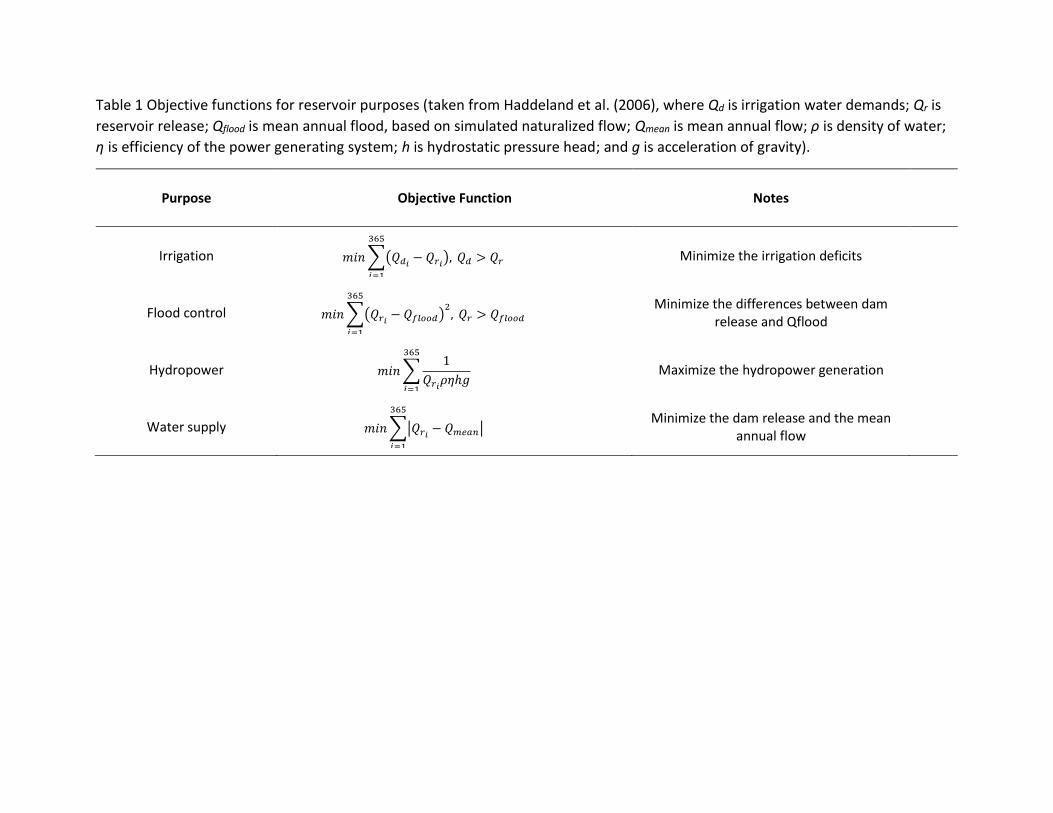
Table 1 Objective functions for reservoir purposes (taken from Haddeland et al. (2006), where Qd is irrigation water demands; Qr is
reservoir release; Qflood is mean annual flood, based on simulated naturalized flow; Qmean is mean annual flow; ρ is density of water;
η is efficiency of the power generating system; h is hydrostatic pressure head; and g is acceleration of gravity).
Purpose Objective Function Notes
Irrigation
Minimize the irrigation deficits
Flood control
Minimize the differences between dam release and Qflood
Hydropower
Maximize the hydropower generation
Water supply
Minimize the dam release and the mean annual flow
𝑚𝑖𝑛 ∑(𝑄𝑟𝑖− 𝑄𝑓𝑙𝑜𝑜𝑑)
2, 𝑄𝑟 > 𝑄𝑓𝑙𝑜𝑜𝑑
365
𝑖=1
𝑚𝑖𝑛 ∑(𝑄𝑑𝑖− 𝑄𝑟𝑖
), 𝑄𝑑 > 𝑄𝑟
365
𝑖=1
𝑚𝑖𝑛 ∑1
𝑄𝑟𝑖𝜌𝜂ℎ𝑔
365
𝑖=1
𝑚𝑖𝑛 ∑|𝑄𝑟𝑖− 𝑄𝑚𝑒𝑎𝑛|
365
𝑖=1

Table 2 The total of 23 simulated reservoirs with satellite estimates (Gao et al. 2012), ranked by capacity.
Reservoir Capacity
(km3) Dam
Dam Location (lat, long)
Basin
Nasser 162 High Aswan 23.97, 32.88 Nile
Guri 135 Guri 7.76, -63 Orinoco
Williston 74 W.A.C. Bennett 56.01, -122.2 Mackenzie
Krasnoyarsk 73 Krasnoyarsk 55.5, 92 Yenisei
Tucurui 50 Tucurui -3.88, -49.74 Tocantins
Tharthar 44 Tharthar 33.79, 43.58 Shatt al-Arab
Mead 37 Hoover 36.01, -114.74 Colorado
Sakakawea 30 Garrison 47.5, -101.42 Mississippi
Oahe 29 Oahe 44.45, -100.39 Mississippi
Rybinsk 25 Rybinsk 58.08, 38.75 Volga
Ilha Solteria 25 Ilha Solteira -20, -51 Parana
Powell 25 Glen Canyon 36.94, -114.48 Colorado
Fort Peck 24 Fort Peck 48, -106.42 Mississippi
Toktogul 20 Toktogul 41.78, 72.83 Amu Darya
Kainji 15 Kainji 10.4, 4.55 Niger
Kremenchuk 14 Kremenchuk 49.08, 33.25 Dnieper
Nova Ponte 13 Nova Ponte -19.15, -47.33 Parana
Mosul 13 Mosul 36.63, 42.82 Shatt al-Arab
Qadisiyah 11 Haditha 34.21, 42.36 Shatt al-Arab
Karakaya 10 Karakaya 38.5, 38.5 Shatt al-Arab
Novosibirskoye 9 Novosibirskoye 54.5, 82 Ob
Chardara 7 Chardara 41, 68 Amu Darya
Roseires 3 Roseires 11.6, 34.38 Nile

Table 3 Summary of the simulated and projected reservoirs in 32 basins.
Continent Basin Number of Simulated
Reservoirs Capacity Simulated
(km3) Total Reservoir Number
in Basin Basin Total Capacity
(km3) Projection Factor
North America
Colorado 3 75 81 91 1.22
Columbia 7 72 127 109 1.52
La Grande 4 164 5 166 1.01
Mackenzie 1 84 13 86 1.02
Mississippi 18 179 723 376 2.08
Nelson 5 93 89 118 1.27
South America
Amazon 2 23 8 25 1.08
Orinoco 4 167 17 177 1.06
Parana 26 322 72 357 1.11
Tocantins 2 118 4 120 1.02
Africa
Niger 4 38 58 48 1.27
Nile 4 424 11 427 1.01
Senegal 1 12 3 13 1.08
Volta 1 168 37 173 1.03
Zambezi 3 288 59 293 1.02
Eurasia
Amu Darya 5 61 23 72 1.18
Amur 3 94 7 96 1.02
Brahmaputra 5 71 81 92 1.30
Chao Phraya 4 32 9 35 1.08
Dnieper 4 44 6 49 1.12
Yellow 4 63 49 77 1.22
Indus 5 49 31 55 1.14
Irrawaddy 1 4 11 7 1.85
Krishna 5 38 57 57 1.49
Lena 1 40 3 41 1.01
Mekong 1 8 20 21 2.78
Ob 2 66 5 72 1.09
Shatt al-Arab 13 246 33 260 1.05
Volga 10 217 17 222 1.02
Yangtze 8 123 373 218 1.79
Yenisei 7 468 7 468 1.00
Australia Murray 3 11 56 26 2.22
TOTAL 166 3877 2095 4461 1.15

Table 4 Summary of simulated and projected reservoirs in five major continents.
Continent Number of Simulated Reservoirs
Capacity Simulated
(km3)
Total Reservoir Number in Continent
Total Capacity
(km3)
Projection Factor
North America 38 667 2249 1918 2.94
South America 34 630 304 963 1.56
Africa 13 930 750 1110 1.22
Eurasia 78 1624 3304 2802 1.75
Australia 3 11 255 107 10.00
TOTAL 166 3862 6862 6900 1.79
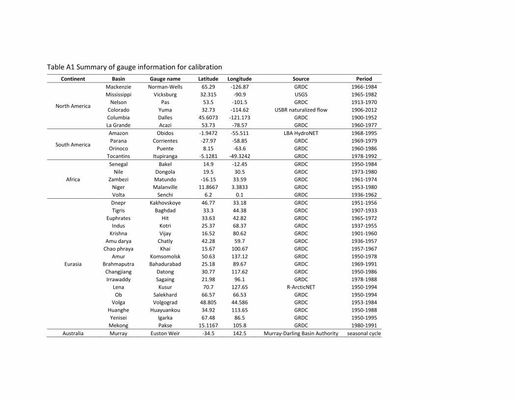
Table A1 Summary of gauge information for calibration
Continent Basin Gauge name Latitude Longitude Source Period
North America
Mackenzie Norman-Wells 65.29 -126.87 GRDC 1966-1984
Mississippi Vicksburg 32.315 -90.9 USGS 1965-1982
Nelson Pas 53.5 -101.5 GRDC 1913-1970
Colorado Yuma 32.73 -114.62 USBR naturalized flow 1906-2012
Columbia Dalles 45.6073 -121.173 GRDC 1900-1952
La Grande Acazi 53.73 -78.57 GRDC 1960-1977
South America
Amazon Obidos -1.9472 -55.511 LBA HydroNET 1968-1995
Parana Corrientes -27.97 -58.85 GRDC 1969-1979
Orinoco Puente 8.15 -63.6 GRDC 1960-1986
Tocantins Itupiranga -5.1281 -49.3242 GRDC 1978-1992
Africa
Senegal Bakel 14.9 -12.45 GRDC 1950-1984
Nile Dongola 19.5 30.5 GRDC 1973-1980
Zambezi Matundo -16.15 33.59 GRDC 1961-1974
Niger Malanville 11.8667 3.3833 GRDC 1953-1980
Volta Senchi 6.2 0.1 GRDC 1936-1962
Eurasia
Dnepr Kakhovskoye 46.77 33.18 GRDC 1951-1956
Tigris Baghdad 33.3 44.38 GRDC 1907-1933
Euphrates Hit 33.63 42.82 GRDC 1965-1972
Indus Kotri 25.37 68.37 GRDC 1937-1955
Krishna Vijay 16.52 80.62 GRDC 1901-1960
Amu darya Chatly 42.28 59.7 GRDC 1936-1957
Chao phraya Khai 15.67 100.67 GRDC 1957-1967
Amur Komsomolsk 50.63 137.12 GRDC 1950-1978
Brahmaputra Bahadurabad 25.18 89.67 GRDC 1969-1991
Changjiang Datong 30.77 117.62 GRDC 1950-1986
Irrawaddy Sagaing 21.98 96.1 GRDC 1978-1988
Lena Kusur 70.7 127.65 R-ArcticNET 1950-1994
Ob Salekhard 66.57 66.53 GRDC 1950-1994
Volga Volgograd 48.805 44.586 GRDC 1953-1984
Huanghe Huayuankou 34.92 113.65 GRDC 1950-1988
Yenisei Igarka 67.48 86.5 GRDC 1950-1995
Mekong Pakse 15.1167 105.8 GRDC 1980-1991
Australia Murray Euston Weir -34.5 142.5 Murray-Darling Basin Authority seasonal cycle

Figure 1 Model simulated basins and reservoirs.

Figure 2 Calibrated seasonal runoff compared with naturalized/undammed streamflow at gauge location for 32 simulated basins.

Figure 3 Simulated seasonal reservoir storage compared with satellite estimates derived by Gao et al. (2012). Comparison period is
provided in each subplot.

Figure 4 Seasonal storage variation for 32 global basins.

Figure 5 The seasonal reservoir storage ([Sr]) compared with seasonal SWE ([Sswe]) and soil moisture ([Ssoil]) in 11 snow significant
basins where range of [Sswe] is greater than 50% of [Ssoil] (a) and the entire 32 simulated basins (b).

Figure 6 The seasonal reservoir variation (Δr) as fraction (F) of natural storage variation (Δn) for 32 basins.

Figure 7 Ternary plot for the 32 simulated basins. The variation of the storage terms (SWE, soil moisture, and reservoir) for each
basin were normalized to sum of one. Color of each point represent the ratio (F) of reservoir variation and natural variation (Δr / Δn).

Figure 8 The seasonal reservoir storage ([Sr]) compared with seasonal SWE ([Sswe]) and soil moisture ([Ssoil]) in Northern (a) and
Southern (b) Hemisphere and five continents (c-g).
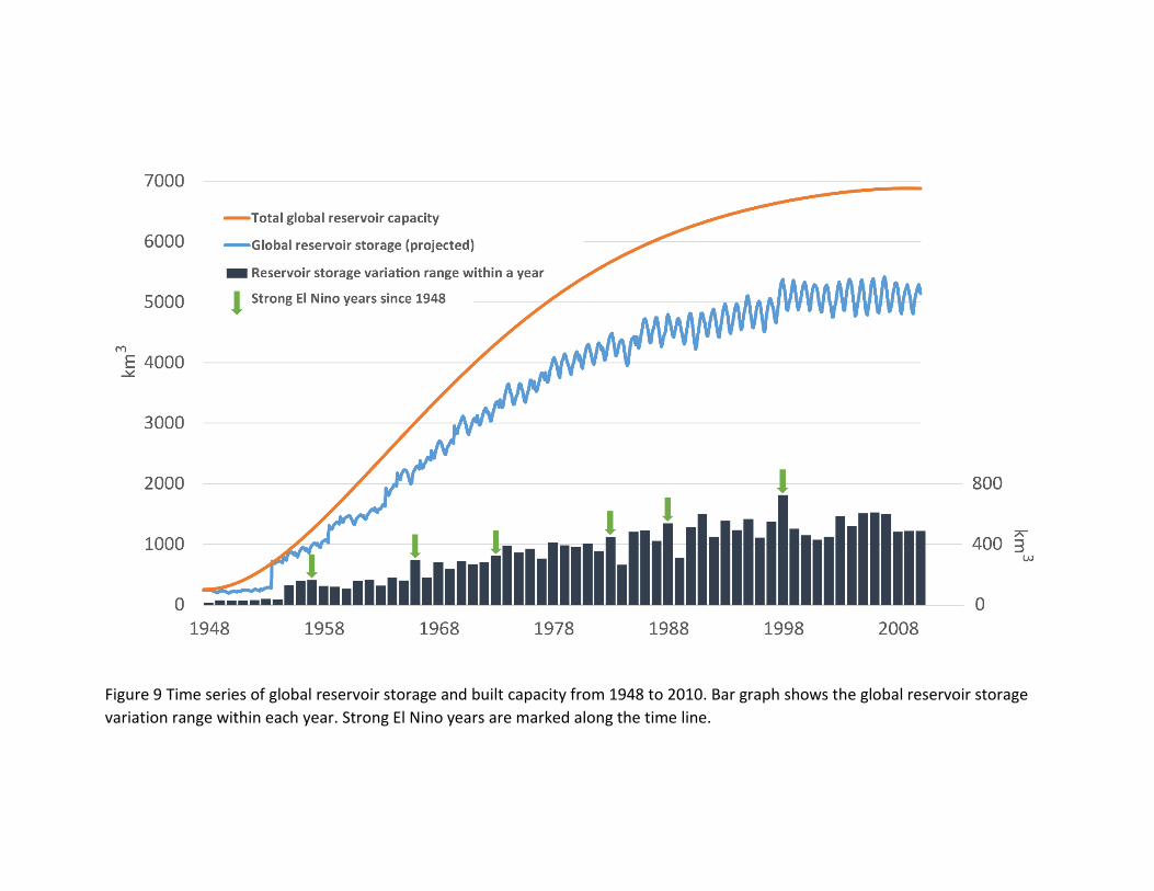
Figure 9 Time series of global reservoir storage and built capacity from 1948 to 2010. Bar graph shows the global reservoir storage
variation range within each year. Strong El Nino years are marked along the time line.

Figure 10 Variation ranges for reservoir storage, soil moisture, and SWE in Northern and Southern Hemispheres calculated by two
different methods.

Figure A1 The seasonal reservoir storage ([Sr]) compared with seasonal SWE ([Sswe]) and soil moisture ([Ssoil]) in 32 simulated basins.

Figure A2 The seasonal reservoir variation (Δr) as fraction of basin annual runoff for 32 basins

Figure A3 Seasonal reservoir storage variation for five continents.


