Tabrizi, Ali Akbar and Al-Bugharbee, Hussein and Trendafilova, Irina and
Garibaldi, Luigi (2016) A cointegration-based monitoring method for
rolling bearings working in time-varying operational conditions.
Meccanica. pp. 1-17. ISSN 0025-6455 , http://dx.doi.org/10.1007/s11012-
016-0451-x
This version is available at https://strathprints.strath.ac.uk/56778/
Strathprints is designed to allow users to access the research output of the University of
Strathclyde. Unless otherwise explicitly stated on the manuscript, Copyright © and Moral Rights
for the papers on this site are retained by the individual authors and/or other copyright owners.
Please check the manuscript for details of any other licences that may have been applied. You
may not engage in further distribution of the material for any profitmaking activities or any
commercial gain. You may freely distribute both the url (https://strathprints.strath.ac.uk/) and the
content of this paper for research or private study, educational, or not-for-profit purposes without
prior permission or charge.
Any correspondence concerning this service should be sent to the Strathprints administrator:
The Strathprints institutional repository (https://strathprints.strath.ac.uk) is a digital archive of University of Strathclyde research
outputs. It has been developed to disseminate open access research outputs, expose data about those outputs, and enable the
management and persistent access to Strathclyde's intellectual output.
A cointegration-based monitoring method for rolling bearings working in
time-varying operational conditions
Ali akbar Tabrizi¹, Hussein Al-Bugharbee², Irina Trendafilova², Luigi Garibaldi³
1) Manufacturing Group, IKID University of Applied Science and Technology, Iran
2) DASM Group, Department of Mechanical and Aeronautical Engineering, University of Strathclyde, UK
3) DIRG Group, Department of Mechanical and Aerospace Engineering, Politecnico di Torino, Italy
Corresponding author:
Ali akbar Tabrizi
Manufacturing Group, IKID University of Applied Science and Technology, 5th km Karaj- Qazvin freeway, Karaj, Iran
Email: [email protected]
Abstract
Most conventional diagnostic methods for fault diagnosis in rolling bearings are able to work only for the case
of stationary operating conditions (constant speed and load), whereas, bearings often work at time-varying
conditions. Some methods have been proposed for damage detection in bearings working under time-varying
speed conditions. However, their application might increase the instrumentation cost because of providing a
phase reference signal. Furthermore, some methods such as order tracking methods can only be applied for
limited speed variations.
In this study, a novel combined method for fault detection in rolling bearings based on cointegration is proposed
for the development of fault features which are sensitive to the presence of defects while in the same time they
are insensitive to changes in the operational conditions. The method makes use solely of the measured vibration
signals and does not require any additional measurements while it can identify defects even for considerable
speed variations. The signals acquired during run-up condition are decomposed into zero-mean modes called
intrinsic mode functions using the Performance Improved Ensemble Empirical Mode Decomposition method.
Then, the cointegration, which is finding stationary linear combination of some non-stationary time series, is
applied to the intrinsic mode functions to extract stationary residuals. The feature vectors are created by
applying the Teager-Kaiser energy operator to the obtained stationary residuals. Finally, the feature vectors of
the healthy bearing signals are utilized to construct a separating hyperplane using the one-class support vector
machine method. Eventually the proposed method was applied to vibration signals measured on an experimental
bearing test rig. The results confirm that the method can be successfully applied to distinguish between healthy
and faulty bearings even if the shaft speed changes dramatically.
Keywords
Rolling bearings fault detection, Teager-Kaiser energy operator (TKEO), one-class support vector machine,
performance improved ensemble empirical mode decomposition (PIEEMD), cointegration, time-varying
operating conditions
1. Introduction
Many research efforts have been focused on fault diagnosis and detection of rolling bearings, since they
constitute one the most important elements of rotating machinery. Most of the diagnostic methods that have
been developed up to date can be applied for the case of stationary working conditions only (constant speed and
load). Randall and Antoni [1] treat broadly the background of some powerful diagnostic methods for roller
bearings in a very useful tutorial paper. However, bearings often work at time-varying conditions such as wind
turbine supporting bearing, mining excavator bearing, run-up and run-down processes. Damage identification
for bearings working under non-stationary operating conditions, especially for early/small defects, requires the
use of appropriate techniques, which are generally different from those used for the case of stationary
conditions, in order to extract fault-sensitive features which are at the same time insensitive to operational
condition variations. So far, some diagnostic techniques have been proposed for time-varying conditions.
Among them, the order tracking method has been widely used for cases of speed variations. But there are still
two main drawbacks of the order tracking method: limitation on the speed variation and the additional
measurement costs introduced by providing the phase signal. The method can effectively detect faults when the
speed variation is limited and an extra device, such as an encoder or a tachometer has to be used to provide a
phase reference signal. Thus, many studies suggest the improvement of the order tracking method [2-7] and its
development so that it can be applied tacho-less [8-9]. Li et al. [10] presented a method based on order tracking
and Teager-Huang Transform (THT) for detection of bearing faults in gearbox under non-stationary run-up of
gear drives. Then, Li [11] combined computed order tracking technique with bi-spectrum analysis. In both
methods a speed transducer was used to measure rotational speed. Urbanek et al. [12] introduced the method
called averaged instantaneous power spectrum as a time–frequency representation of selected cyclic
components and tested on a selected case of wind turbine drive train fault. However, they believed that
averaging can be applied when dealing with limited fluctuations of operational conditions. Cocconcelli et al.
[13] applied another method for damage detection of roller bearing in direct-drive motors. They used the
marginal time integration of the averaged Short Ttime Fourier transform (STFT) spectrogram as a simple
indicator of damage. As the AC motor was controlled by a drive, they were able to use the speed profile in their
methodology. They also applied the spectral kurtosis and the energy distribution for damage identification of a
brushless AC motor using the angular velocity [14].
However, for the discussed methods, recording the speed requires additional instrumentation, which
increases the measurement and the computational costs and adjustment problems.
In another approach, Zimroz et al. [15] used a two dimensional space made of the peak-to-peak amplitude
of vibration signal and the generated power for diagnosis of the main bearing of a wind turbine working under
non-stationary conditions. However, in most applications, there is no additional data that can be measured
during the process (as e.g. the generated power) apart from the measured acceleration signals. And it should be
kept in mind that for the case of wind turbines, the speed variation of the bearings is limited and called
fluctuation (less than 30% [16]) in comparison with some time-varying conditions such as fast run up
conditions.
Cointegration is a statistical concept which can be used for testing the existence of statistically significant
relation between two or more non-stationary time series. It is looking for linear stationary combinations within
non-stationary time series. Engle and Granger [17] formulated one of the first tests for cointegration. Johanson
proposed a maximum likelihood approach for finding stationary linear combinations of non-stationary
variables, which have the same order of integration [18]. Applications of cointegration to finance may be found
in [19-23]. Cointegration has been recently applied for structural health monitoring (SHM) purposes to remove
the non-stationarity produced by environmental variations such as temperature, wind and humidity [24-27].
Cross and Worden discussed the application of cointegration to engineering data [25]. Cross et al. [26]
successfully applied cointegration for SHM purposes, where it was used to detect the introduction of damage
in a composite plate. Antoniadou et al. applied the Hilbert-Huang and Teager- Kaiser transforms to extract
relevant information from the acquired signals and subsequently used cointegration to remove the non-
stationarity produced by variation of the environmental conditions [24]. Worden et al. demonstrated how a
multi-resolution approach to cointegration can enhance the damage assessment capability for the case of a
composite plate [27].
The Teager-Kaiser energy based feature extraction method proposed by Tabrizi et al [39] is able to
successfully identify the early damage level of roller bearings operating in stationary conditions. In this study
a new approach is proposed to detect the state of rolling bearings operating in conditions of time-varying speed.
Contrary to the afore-mentioned methods, we collected only acceleration signals and it does not require any
additional measurements and/or instrumentation. Furthermore, it works even for cases when the speed changes
rapidly (for example in a run-up start). The methodology is introduced in two parts, signal analysis and pattern
recognition. The signal acquired is divided into segments and each segment is broken down into some
elementary modes the Intrinsic Mode Functions (IMFs) using the Performance Improved Ensemble Empirical
Mode Decomposition (PIEEMD) proposed by some of the authors of this study for stationary operating
condition [28]. Then, three dimensional feature vectors are created by applying the Teager-Kaiser Energy
Operator (TKEO) to the cointegrated residuals of the first three IMFs. The feature vectors obtained from healthy
bearing signals are further utilized as input to construct a separating hyperplane for a one-class Support Vector
Machine (SVM). The SVM can be trained to categorize signals coming from healthy and faulty bearings. It is
shown that the proposed method can successfully identify signals from healthy and faulty bearings.
The rest of the paper is organized as follows:
Signal analysis and pattern recognition (one-class SVM) methods are introduced in section 2.1 and 2.2,
respectively. The whole process for roller element bearing fault detection is explained in 2.3. The experimental
setup and the data-acquisition process are presented in section 3. The application of the new approach to the
acquired data together with some results is discussed in section 4. Eventually, the paper concludes with a
discussion in section 5.
2.1 .Signal analysis
In order to extract signal features each collected signal is divided into segments. Then, several methods are
applied. The signal analysis techniques are detailed below.
2.1.1. Segmentation
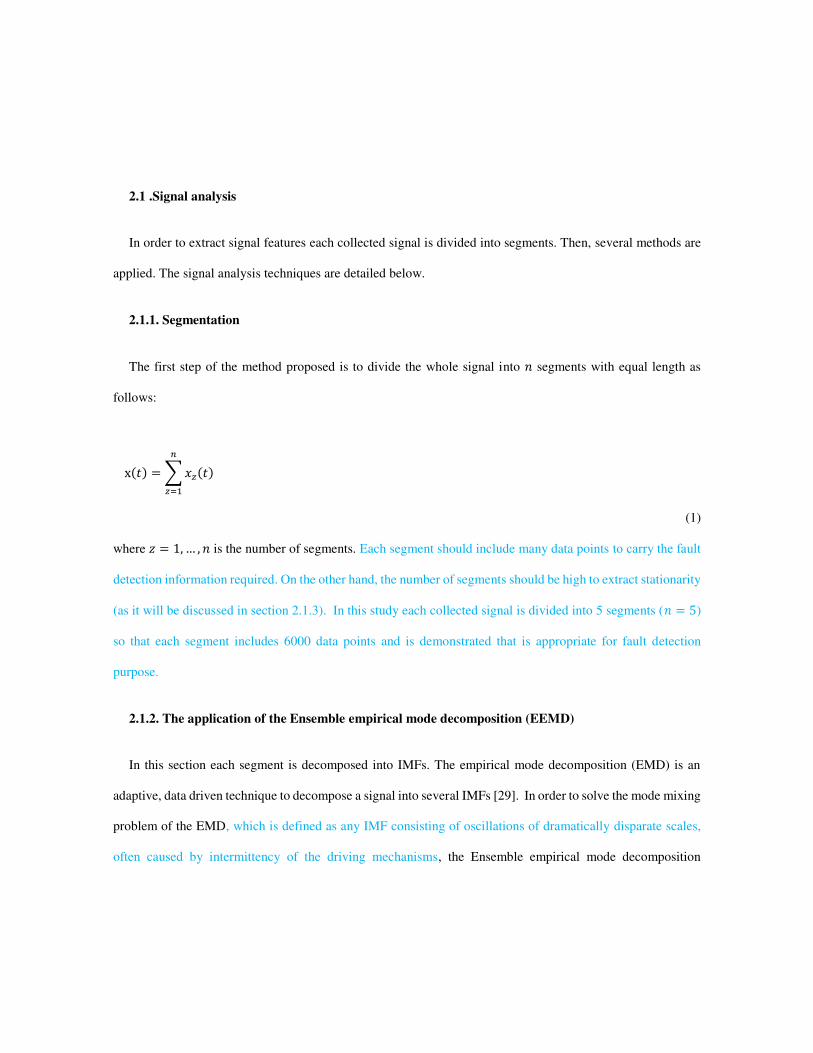
The first step of the method proposed is to divide the whole signal into 券 segments with equal length as
follows:
x岫建岻 噺 布 捲佃岫建岻津佃退怠
(1)
where 権 噺 な┸ ┼ ┸ 券 is the number of segments. Each segment should include many data points to carry the fault
detection information required. On the other hand, the number of segments should be high to extract stationarity
(as it will be discussed in section 2.1.3). In this study each collected signal is divided into 5 segments (券 噺 の)
so that each segment includes 6000 data points and is demonstrated that is appropriate for fault detection
purpose.
2.1.2. The application of the Ensemble empirical mode decomposition (EEMD)
In this section each segment is decomposed into IMFs. The empirical mode decomposition (EMD) is an
adaptive, data driven technique to decompose a signal into several IMFs [29]. In order to solve the mode mixing
problem of the EMD, which is defined as any IMF consisting of oscillations of dramatically disparate scales,
often caused by intermittency of the driving mechanisms, the Ensemble empirical mode decomposition
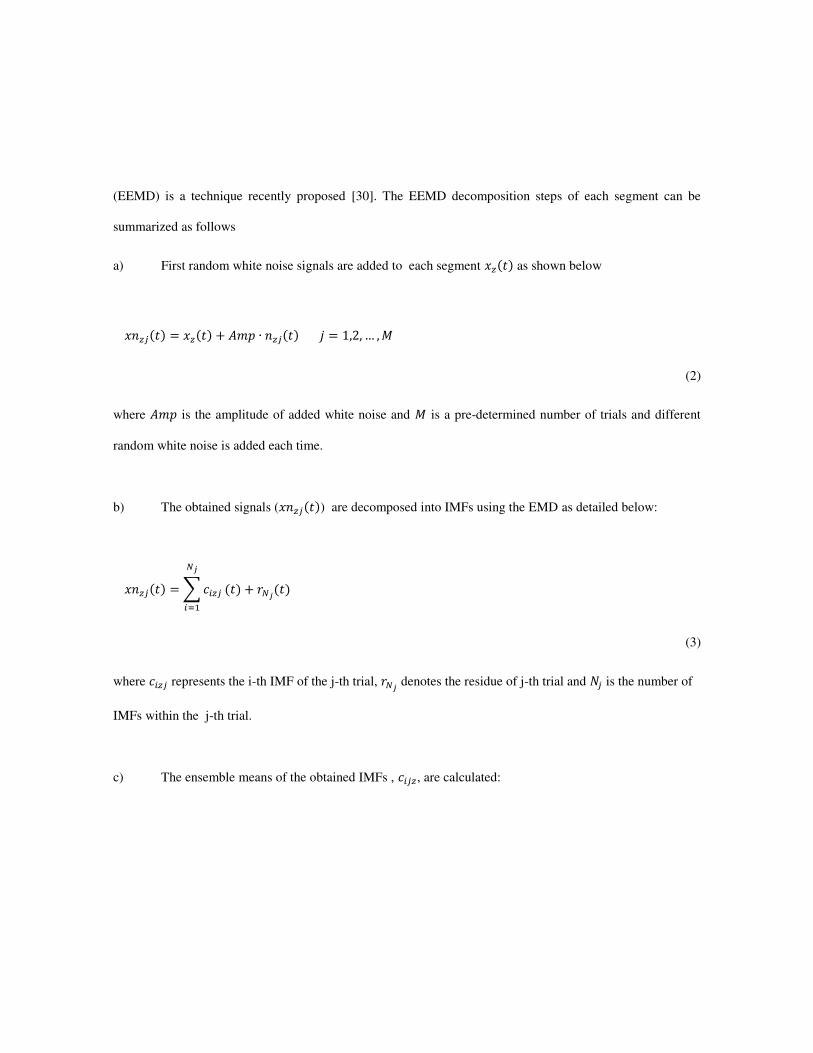
(EEMD) is a technique recently proposed [30]. The EEMD decomposition steps of each segment can be
summarized as follows
a) First random white noise signals are added to each segment 捲佃岫建岻 as shown below
捲券佃珍岫建岻 噺 捲佃岫建岻 髪 畦兼喧 ゲ 券佃珍岫建岻 倹 噺 な┸に┸ ┼ ┸ 警
(2)
where 畦兼喧 is the amplitude of added white noise and 警 is a pre-determined number of trials and different
random white noise is added each time.
b) The obtained signals (捲券佃珍岫建岻) are decomposed into IMFs using the EMD as detailed below:
捲券佃珍岫建岻 噺 布 潔沈佃珍朝乳
沈退怠 岫建岻 髪 堅朝乳岫建岻
(3)
where 潔沈佃珍 represents the i-th IMF of the j-th trial, 堅朝乳 denotes the residue of j-th trial and 軽珍 is the number of
IMFs within the j-th trial.
c) The ensemble means of the obtained IMFs , 潔沈珍佃, are calculated:
荊警繋沈佃岫建岻 噺 嵜布 潔沈珍佃暢珍退怠 崟 警板
(4)
where 件 噺 な┸に┸ ┼ ┸ 詣, 警 is the minimum number of IMFs among all the trials and z is segment number. Thus,
for example, 荊警繋怠怠┸ ┼ ┸ 荊警繋挑怠 are the L IMFs obtained by decomposing the first segment and 荊警繋怠態┸ ┼ ┸ 荊警繋挑態
are the L IMFs obtained by decomposing the second segment and so on.
Adding noise aims to affect the extrema of the original signal so that the intermittency of the components will
be removed. In order to improve the performance of the EEMD, an adaptive method called Performance
Improved EEMD (PIEEMD) was proposed by Tabrizi et al. [28] to determine the appropriate amplitude of
added noise. After adding a random white noise, by applying the signal to noise ratio (SNR) definition (see
equation (5)), the amplitude value for each data point of a segment is obtained using equation (6). The SNR is
considered as a constant predetermined value (SNR=10) in equation (6).
鯨軽迎 噺 にど log 岫Signal amplitude 軽剣件嫌結 欠兼喧健件建憲穴結エ 岻
(5)
畦兼喧佃珍岫建岻 噺 など貸岫聴朝眺態待 岻 盤捲佃岫建岻【券佃珍岫建岻匪
(6)
where z corresponds to the segment , z = 1,2…n and j=1,2.., M is the number of trials.
2.1.3. Cointegration
The cointegration technique is used to find linear stationary combination of the corresponding IMFs
(obtained in section 2.1.2.). Two or more non-stationary time series (with the same integrated order) are said to
be cointegrated if a linear combination of them is stationary. A signal/stochastic process 姿嗣 is said to be
integrated of order d (姿嗣b薩岫纂岻), if it becomes stationary after d times differencing. Thus, a time series 姿嗣 will
be integrated of order 1, if its first difference is stationary (ッ姿嗣b薩岫宋岻). The order of integration can be estimated
by a stationarity test using the Augmented Dickey-Fuller (ADF) test [31].
Now we will form new signals 桁沈痛 from the obtained IMFs. A signal 桁沈痛 is made of n non-stationary IMFs
(荊警繋沈怠┸ ┼ ┸ 荊警繋沈津) obtained from the n signal segments xn (see equation (4)).
桁沈痛 噺 蕃荊警繋沈怠教荊警繋沈津否
(7)
where 件 噺 な┸ ┼ ┸ 兼 is the order of IMFs and 兼 is the number of IMFs selected. For example, when 件 噺 な, it
means that 桁怠痛 is made of the first IMFs of all n segments 岫荊警繋怠怠┸ ┼ ┸ 荊警繋怠津岻 and when 件 噺 な, 桁態痛 is made of
second IMFs of all segments岫荊警繋態怠┸ ┼ ┸ 荊警繋態津岻.
The series 桁沈痛 is said to be cointegrated with r cointegrating vectors (0 < r < n) if there exists a (n×r) matrix 紅
such that the cointegrating residual 憲 is 0 integrated.
紅嫗桁沈痛 噺 蕃紅怠嫗桁沈痛教紅追嫗 桁沈痛否 噺 蕃憲沈怠教憲沈追否
(8)
Where 紅嫗 is introduced as transpose of 紅.
The cointegration test based on Johansen procedure [18], tests for the existence of r, 0 ≤ r < n, cointegrating
vectors (紅怠┸ ┼ ┸ 紅追岻. It determines which of the cointegrating vectors creates the most stationary linear
combination.
In order to find the cointegrating vectors, first we establish the residuals of the following regressions:
ッ桁沈痛 噺 布 も怠痛嫦ッ桁沈岫痛貸痛嫦岻 髪 戟撫沈痛椎痛嫦退怠
(9)
桁沈岫痛貸怠岻 噺 布 も態痛嫦ッ桁沈岫痛貸痛嫦岻 髪 撃侮沈痛椎痛嫦退怠
(10)
where 喧 denotes the model order, 戟撫痛 and 撃侮痛 denote the residuals and も怠 and も態 are multiplication matrices.
Then, the cointegrating vectors are determined as eigenvectors of the following eigenvalue problem:
】膏沈鯨沈怠怠 伐 鯨沈怠待鯨沈待待貸怠鯨沈待怠】 噺 ど
(11)
where 鯨沈待待 噺 怠脹 デ 戟撫沈痛戟撫沈痛嫗脹痛退怠 , 鯨沈待怠 噺 怠脹 デ 戟撫沈痛撃侮沈痛嫗脹痛退怠 , 鯨沈怠待 噺 怠脹 デ 撃侮沈痛戟撫沈痛嫗脹痛退怠 , 鯨沈怠怠 噺 怠脹 デ 撃侮沈痛撃侮沈痛嫗脹痛退怠 are the sample
covariance matrices.
The eigenvector corresponding to the largest eigenvalue is the most stationary cointegration vector. The test
statistic (see equation (12)) is applied to test the hypothesis.
Tstat沈 岫堅待岻 噺 伐劇 布 ln 岫な 伐 膏實沈槌眺槌退追轍袋怠 岻
(12)
where 件 噺 な┸ ┼ ┸ 兼 is the order of IMFs and 兼 is the number of IMFs selected, 膏實沈槌 denotes the estimated
eigenvalues and 迎 is the number of eigenvalues obtained from equation (11).
P-value is defined as the right-tail probabilities of the test statistics. Thus, it is the probability under the
assumption of the null hypothesis. The null hypothesis is rejected if the P-value is less that a pre-determined
significance level, which is usually set to 5% (0.05). The critical values, tabulated by Johansen [18], were
calculated based on 5% P-value. In this case, the null hypothesis is rejected, when the trace statistic value
become less than critical value.
First the null hypothesis (H待岫堅待 噺 ど岻) is tested against the alternative hypothesis (H怠岫堅待 伴 ど岻岻. If the null
hypothesis is accepted then there are no cointegrating vectors. If the null hypothesis is rejected then there is at
least one cointegration vector and the test is continued to test H待岫堅待 噺 な岻 against H怠岫堅待 伴 な岻. There exists only
one cointegrating vector, if the null hypothesis is accepted. Otherwise, it is concluded that there are at least two
cointegrating vectors. The procedure is continued until the null hypothesis is accepted.

2.1.4. Teager-Kaiser Energy Operator (TKEO)
The energy of a signal is the sum of squared absolute value of the signal over a time, which is not the
instantaneous summed energy. Kaiser observed that a second order differential equation is the energy required
to generate a simple sinusoidal signal varies with both amplitude and frequency [32]. In order to estimate the
instantaneous energy of a signal x(t), Teager-Kaiser Energy Operator (TKEO) is used as an energy tracking
operator as follows (Maragos, 1993): 皇岷捲岫建岻峅 噺 畦態 噺 捲岌 態岫建岻 伐 捲岫建岻 捲岑 岫建岻
(13)
where )(tx and )(tx are the first and the second time derivatives of x(t), respectively.
For a discrete signal, using differences to approximate differentiation, the TKEO can be developed as [33]: 閤範憲沈珍岫建岻飯 噺 憲沈珍態岫建岻 伐 憲沈珍岫建 髪 な岻 憲沈珍岫建 伐 な岻
(14)
where 建 is the discrete time index.
As at any instant, only three consecutive values are needed to estimate the instantaneous TKEO, it is adaptive
to the instantaneous changes in signals and is able to resolve transient events.
In the method proposed the TKEO is applied to the 堅 stationary cointegrated residuals岫憲沈怠 ┼ 憲沈追岻 obtained
in section 2.1.3. The sum would be a value and is obtained as follows:
劇計継沈珍 噺 布 閤盤憲沈珍匪
(15)
where 件 噺 な┸ ┼ ┸ 兼 is the number of IMFs selected and 倹 噺 な┸ ┼ ┸ 堅 is the number of cointegrated residuals.
2.1.5. Creating feature vectors
Feature vectors used as input for the consequent pattern recognition method are formed based on the values
calculated in equation (15). In this study three IMFs are selected, in order to have enough information and on
the other hand less dimensional feature vectors [34].
繋珍 噺 岷劇計継怠珍 劇計継態珍 劇計継戴珍峅 (16)
where 倹 噺 な┸ ┼ ┸ 堅 is the number of cointegrated residuals. For example, 繋怠 is the three dimensional feature
vector created using the first residual and 繋態 is the feature vector created using the second residual. Thus, for
each signal we find r feature vectors.
Then, the feature vectors obtained are normalized by dividing them to their Euclidean norm as follows:
繋撃券珍 噺 岷劇計継怠珍【券剣堅兼岫劇計継怠珍岻 劇計継態珍【券剣堅兼岫劇計継態珍岻 劇計継戴珍【券剣堅兼岫劇計継戴珍岻峅 (17)
Which can be represented as follows so that each dimension would be a value: 繋撃券珍 噺 岷繋撃怠珍 繋撃態珍 繋撃戴珍峅 (18)
2.2. Pattern recognition
In this part a pattern recognition method is applied in order to recognize between healthy and faulty bearing
or rather the signals that come from them. For the purpose the one class support vector machine method is
applied. The method is briefly described below.
2.2.1. One-class support vector machine
The support vector machine (SVM) introduced by Vapnik is a relatively new computational learning
statistical PR method based on statistical learning theory [35]. It is applied for recognizing between two classes-
healthy and faulty signals. The method requires a relatively small training samples for the learning phase. Thus,
the method accommodates the fact that acquiring a sufficient number of faulty signals is not applicable in
practice, and it has been successfully used in a number of fault diagnosis problems. The one-class SVM
Insert [Figure 2- Classification by one-class SVM (from [36])] somewhere here
proposed by Scholkopf et al. is a powerful technique which constructs a separating hyperplane between two
classes of patterns using data from one of the classes only. It classifies the patterns from the other class as
outliers [37]. It constructs a hyperplane around the data, such that its distance to the origin (called Margin) is
maximal among all possible hyperplanes and can be adopted for anomality detection, as shown in Figure 2.
For each residual, the feature vectors 繋撃券珍 obtained from the healthy bearing signals (using equation (18))
are used to construct the hyperplane. As there are a number of features for each residual, we use l 繋撃券珍賃 vectors
as features, where 倹 denotes residual number and 倦 噺 な┸ ┼ ┸ 健 is the feature number used for training.
The SVM can be also applied in case of non-linear classification by mapping the data onto a high dimensional
feature space (剛盤繋撃券珍賃匪), where the linear classification is then possible. In real problems, an exact line
dividing the data is usually difficult to obtain, so, by introducing the slack variable (行賃岻 in equation (19) and
ignoring few outlier data points a smooth boundary can be created.
The Margin is defined as [37]:
警欠堅訣件券 噺 貢 押拳押エ
(19)
where 拳 and 貢 are the weight vector and the offset parameterizing the hyperplane.
In order to separate the data set from the origin, the following quadratic optimization problem must be solved
[37]:
minimize 蕃なに 押拳押態 髪 な鉱健 布 行賃鎮賃退怠 伐 貢否
(20)
subject to 崕検賃 岾拳 ゲ 剛盤繋撃券珍懲匪峇 半 貢 伐 行賃行賃 半 ど
where 倹 噺 な┸ ┼ ┸ 堅 is the number of residuals, 倦 噺 な┸ ┼ ┸ 健 is the features used to train the model, 検賃 is a vector
includes the label of each feature (+1 for the features of healthy bearing signals and -1 for the features of faulty
bearing signals) , 行賃 is the slack variable and measuring the distance between the hyperplane and the examples

that laying in the wrong side of the hyperplane (Figure 3), 鉱 is the regularization parameter and represents an
upper bound on the fraction of outliers (training errors) and a lower bound on the fraction of support vectors
(the nearest features to the hyperplane) with respect to the number of training samples. It is a variable taking
values between 0 and 1 that monitors the effect of outliers (hardness and softness of the boundary around data).
By applying a kernel function as the inner product of mapping functions (計盤繋撃券珍賃┸ 繋撃券珍賃 ┸匪 噺 岫剛盤繋撃券珍賃匪 ゲ剛盤繋撃券珍賃┸匪岻, it is not necessary to explicitly evaluate mapping in the feature space, where ┸ 倦 ┸ 噺 な┸ ┼ ┸ 健 . Various
kernel functions can be used, such as linear, polynomial or Gaussian RBF (Radial basis function). In this study,
RBF kernel function, a common function in fault detection problems, is applied:
計盤繋撃券珍賃 ┸ 繋撃券珍賃┸匪 噺 結捲喧 岾伐紘舗繋撃券珍賃 伐 繋撃券珍賃┸舗態峇
(21)
Insert [Figure 3- The slack variables 行沈 and support vectors (data points with circles around them) (from
[38]).] somewhere here
Introducing Lagrange multipliers the dual problem is formulated as:
兼件券件兼件権結 なに 布 糠賃糠賃 ┸鎮賃┸賃┸退怠 計盤繋撃券珍賃┸ 繋撃券珍賃 ┸匪
(22)
subject to 崕 ど 判 糠賃 判 怠鄭鎮デ 糠賃鎮賃退怠 噺 な
If 鉱 approaches 0, the upper boundaries on the Lagrange multipliers tend to infinity, so the second inequality
constraint in (equation (22)) becomes void. Furthermore, the penalty for errors becomes infinite, so the
algorithm returns to the corresponding hard margin algorithm.
The feature vectors (FV) which achieve positive, non-zero multipliers called support vectors 鯨撃珍沈 where 件 corresponds the number of support vectors (SV). Then, offset is calculated as follows:
貢 噺 岫拳 ゲ 剛盤鯨撃珍沈匪岻 噺 布 糠賃鎮賃退怠 計盤繋撃券珍賃 ┸ 鯨撃珍沈匪
(23)
Accordingly the non-linear decision function for labelling new samples 繋撃券珍 is represented as follows:
血盤繋撃券珍匪 噺 嫌件訣券 蕃布 糠賃鎮賃退怠 計盤繋撃券珍賃 ┸ 繋撃券珍匪 伐 貢否
(24)
The classification parameters (紘 and 鉱), which must be determined, are optimized by using cross validation
method.
2.3. The whole methodology
Eventually the method suggested can be summarized as shown in Figure 3.
Insert [Figure 3- The cointegration based methodology suggested in this study for roller bearing fault
detection working in operational variation condition] somewhere here
3. Method validation and verification
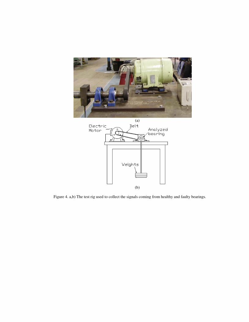
For the purpose of demonstration and validation of the suggested methodology, experimental data (only
acceleration signal) was obtained from the test rig assembled at the DASM Group in the Department of
Mechanical and Aerospace Engineering of Strathclyde University which is shown in Figures 4(a) and (b). As
discussed in section 2.3 we do not require any data except for the acceleration signals. The test rig consists of
a shunt DC motor (1 hp and 2000 rpm), bearing assembly and a mechanical loading system. In order to acquire
acceleration signals, the MONITRAN accelerometer (MTN/1120 model) was fixed to the bearing supports by
magnetic coupling. The bearings used in the experiment were SKF deep grooves 6308. Two bearing conditions
were considered in this study healthy and inner race faulty. The fault was considered a small notch on the inner
ring created using spark erosion to simulate a flaking or spalling fault. The width was considered less than 1mm
and the depth was almost 100 microns. 20 signals were acquired for each bearing condition. Signals were
sampled at 1.3 kHz and each had a 25 seconds time length. For all the acceleration signals acquired, the run up
time varying operating condition was considered by varying the speed manually from 150 to 1500 rpm. Thus,
speed variation considered is significant with different speed rates to demonstrate that the results are
independent to speed rate. The faults considered here were very small notches. Thus, the primary interest of
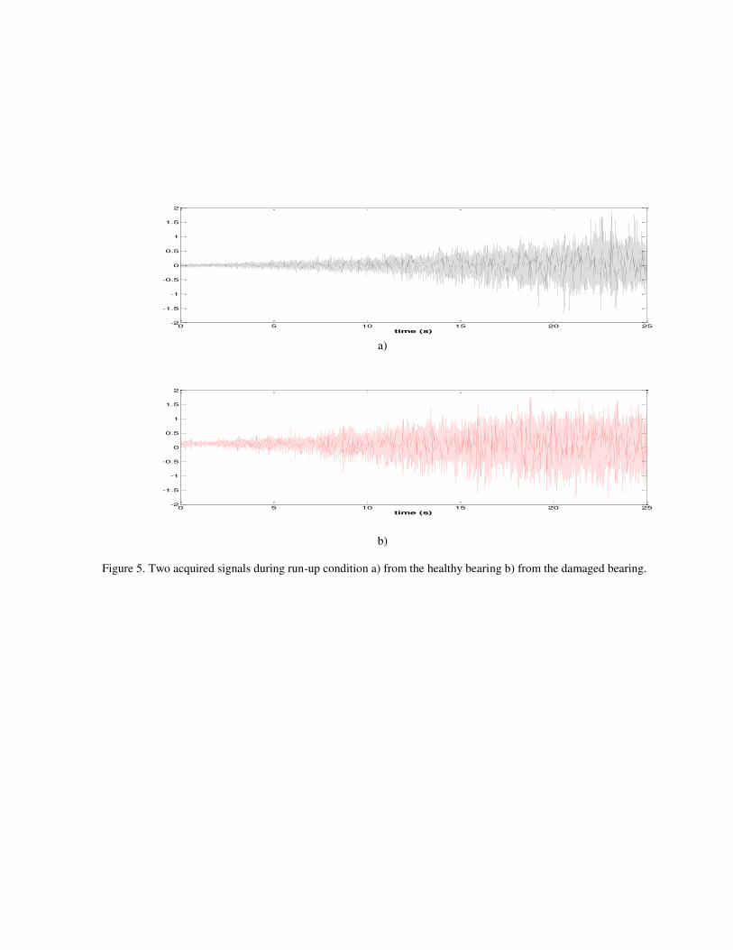
this study is to detect very small faults at a rather early stage. Two acquired signals during run-up condition
from the healthy and damaged bearings are displayed in Figure 5.
The process of the method follows the steps detailed above in section 2.3.
Insert [Figure 4. a,b) The test rig used to collect the signals coming from healthy and faulty bearings.]
somewhere here
Insert [Figure 5. Two acquired signals during run-up condition a) from the healthy bearing b) from the damaged
bearing.] somewhere here
4. Results and discussion
In this section we present and discuss some results from the application of the suggested method. Firstly the
results of the application of the Teager-Kaiser energy (TKE) based feature extraction method proposed by
Tabrizi et al. [39] are provided in order to test the identifiability of the measured signals. Subsequently the
method suggested in this study (cointegration based method) will be applied to the same signals in order to see
the effect of the cointegration residuals on the resulting classification. In the TKE based method [39], a signal
is decomposed into IMFs using the performance improved EEMD (PIEEMD) and then the TKE operator is
applied to the first three IMFs to obtain three dimensional feature vectors. After normalizing, one obtains three
feature vectors called 参皐撮仔層, 参皐撮仔匝 and 参皐撮仔惣. The results of applying TKE based method to the signals
collected in time-varying operating condition (run-up) are shown in Figure 6. The Figure presents all the three
features on a 3d plot (Figure 6(a)) and different combinations of the features 参皐撮仔層, 参皐撮仔匝 and 参皐撮仔惣(Figure 6 (b), (c) and (d)). Although this method is known to be a powerful tool for detection of small
faults, it can be seen that for the case of non-stationary operational conditions the feature vector points are not
well separated and it is impossible to determine the condition of the bearing. Thus in this case for a variable
motor speed the above method fails to provide reliable fault detection.
Insert [Figure 6. The normalized TKE using the combined method consists of PIEEMD (as the decomposition
technique) and TKEO (to create feature vectors).] somewhere here
Secondly, it is investigated if and to what extent the cointegration based method proposed in this study
(section 2.3) is able to recognize the state of the bearings. As detailed in the section 2.3, first, each signal is
divided into five segments so that each segment includes 6000 data points. Then, each segment is decomposed
by the PIEEMD algorithm. The results for healthy and faulty signals are given in Figures 7 and 8. The
cointegration procedure is then carried out for all the five IMFs corresponding to each segment to obtain one or
more cointegrating vectors.
The results of Johansen test for cointegration for the healthy bearing signal (displayed in Figure 5(a)) are
given in Table 1. From Table 1, the results regarding the existence of cointegration relations among a set of
IMFs are given. The table shows that there are four linear combinations of the IMFs labeled under the null ranks
column (i.e r0, r1...r3). The other columns give information whether each of these linear combinations indicates
cointegration among the IMFs or not. The null hypothesis of the test suggests that there is no cointegration
among the IMFs. In this table the h values given in column 2 of Table 1 are all equal to 1, which rejects the null
hypothesis. Consequently, the problem is full ranked since all the null hypothesis are rejected. The right-tail
probabilities Prt (i.e P-values given in column 5) are considerably lower than the significance level (which is
0.05). This indicates that there is enough evidence of the stationarity of the cointegrating vector (since there is
a cointegration relation among the IMFs).
Insert [Figure 7. The IMFs of the first segment of the healthy signal (Figure 5(a)) obtained performance
improved EEMD (PIEEMD).] somewhere here
Insert [Figure 8. The IMFs of the first segment of the faulty signal (Figure 5(b)) obtained using performance
imperoved EEMD (PIEEMD).] somewhere here

Insert [Table 1. The results of cointegration for the first IMFs of five segments of the healthy signal shown in
Figure 5(a)] somewhere here
Insert [Figure 9. The cointegrating vectors obtaind from first IMFs 岫荊警繋怠怠 ┼ 荊警繋怠泰岻 of the five segments
of the signal shown in Figure 5(a).] somewhere here
Insert [Figure 10. The TKEO applied to the cointegrated residuals obtained from 岫荊警繋怠怠 ┼ 荊警繋怠泰岻, 岫荊警繋態怠 ┼ 荊警繋態泰岻 and 岫荊警繋戴怠 ┼ 荊警繋戴泰岻, respectively.] somewhere here
The values of the other parameters in Table 1 (test statistics values, critical values and Eigenvalues) give
information about the stationarity for each cointegration residual. The Eigenvalues are arranged in ascending
order corresponding to the order of null ranks (r0, r1, r2 and r3). The four stationary cointegration residuals are
shown in Figure 9.
Eventually, the TKEO is applied to each cointegration residual (equation (14)), and the results are shown in
Figure 10. The three dimensional feature vectors are created according to equation (15). After normalizing (see
equation (16)), the feature vectors used in the classification process are obtained (equation (17)). Thus, for each
signal, we are in possession of one three dimensional feature vector.
The visualization of the 3-dimensional feature vectors and their projections corresponding to the healthy and
faulty bearings for each cointegration residual are shown in Figures 11 to 14. A very good separation between
the healthy and the faulty classes obtained from the first and the second cointegrated residuals can be
appreciated. For each cointegration relation, there are 20 feature vectors developed for each class. From the
class of healthy bearings, 80% of the feature vectors (i.e 16 out of 20) are used as training input for the one-
class SVM method (see section 2.2.1). Consequently, the constructed hyper-plane is utilized for determining
Insert [Figure 11. The three dimensional feature vectors obtained from first cointegrated residual.] somewhere
here
Insert [Figure 12. The three dimensional feature vectors obtained from the second cointegrated residual.]
somewhere here
Insert [Figure 13. The three dimensional feature vectors obtained from the third cointegrated residual.]
somewhere here
Insert [Figure 14. The three dimensional feature vectors obtained from the fourth cointegrated residual.]
somewhere here
the condition of the new test vectors. The test sample contains the remaining 20% of the healthy and all faulty
feature vectors. Since, the signals were collected in different speed variations, the healthy signals acquired are
different, which means that the training samples (80% of the healthy features) and healthy test samples
(remaining 20% of healthy features) are not similar.
The classification rate is shown in the Table 2. It can be seen that for all the cases (all cointegration residuals),
the success rates for the training and the test samples are 100% when the first and the second cointegration
residuals are used, as this result was expected based on Figures 11 and 12. However, when the third or the
fourth cointegration residuals are used the features vectors from the test sample are not well separated, but the
success rate for the training sample is still 100%. When using the third cointegration residual, there are two
false-positive cases (i.e two healthy samples that are miss-classified as faulty). When the fourth cointegration
residual is used four out of the 24 samples were miss-labeled (one false -positive case and three false-negative
ones (i.e three faulty FV are misclassified as healthy). False-positive yields to implement a maintenance
procedure whereas consequence of false-negative is to run the machine when it is faulty and has to be stopped
to be repaired.
Insert [Table 2. The classification results for different cointegrated residuals] somewhere here
The margin obtained for each classification is also indicated in Table 2. It can be seen that using the feature
vectors obtained from the first or the second residuals vector provides a more reliable hyperplane, as they have
higher margin values, while the margin values for the third and fourth residuals fall down and accordingly the
classification rate deteriorates.
Since the method proposed is anomaly detection (one-class SVM), all data acquired from faulty bearing was
used to test the method. In order to demonstrate the ability of the method, new signals (20 signals) were collected
from a new healthy bearing and based on the results obtained the method recognized perfectly the state new
healthy bearing.
On the basis of the results discussed above it can be appreciated that the implementation of the method
proposed in this study, a very good/ perfect recognition of the bearing state can be achieved, even when the
shaft speed changes significantly.
5. Conclusions
This study proposes a roller element fault detection method, which is based on the statistical concept of
cointegration. The cointegration is used for the purposes of detecting the stationary content of the signal by
finding the linear stationary combinations of its elements. The signal is first divided into segments and each
segment is broken down into elementary modes, the IMFs, using the Performance Improved Ensemble
Empirical Mode Decomposition (PIEEMD). Subsequently, three dimensional feature vectors are created by
applying the Teager-Kaiser Energy Operator (TKEO) to the cointegrated residuals of the first three IMFs.
The suggested method can work for constant operational speed but unlike most other fault detection methods
for roller element bearings it can distinguish between healthy and faulty bearings even when the speed is
significantly changing. Most roller element fault detection methods that can operate in speed varying conditions
require additional instrumentation like e.g a tachometer or encoder. Some of these methods, like the order
tracking one, can detect the damage when the speed variation is limited. The method suggested in this study
does not put any constraints on the speed variation and can work even when the speed changes rapidly (for
example in a run-up start). This is a very important merit of the proposed method since most rotating
machineries operate with time varying speed and the application of this method provides a procedure for online
fault monitoring, without putting the machinery into parts.
This study validates the suggested method by applying it on the data obtained from an experimental setup
operating in run-up condition. The suggested method uses a training pattern recognition procedure in order to
recognize between healthy and faulty bearing signals. 80% of the acquired signals are used for training purposes
and the rest are used as a testing sample.
The results given in the previous paragraph show a 100% correct classification for the signals from the
testing sample and 100% correct classification for the testing sample as well when the most stationary
cointegration residuals (the first and the second one) are used to obtain the feature vectors. When the residuals
with lower/weaker stationarity are used, the results deteriorate slightly but still the majority of the signals are
correctly recognized.
The suggested methodology can be further developed for the purposes of qualification (fault type
recognition) and eventually quantification purposes using the multi class SVM. But even in its proposed state
as a detection method this is the first methodology of such kind which can operate under time varying speed
(run-up) without requiring additional instrumentation.
Acknowledgement
This work has been partially carried out in the framework of the GREAT2020 - phase II, project.
References
[1] Randall RB, Antoni J (2011) Rolling element bearing diagnostics – A tutorial. Mechanical Systems and
Signal Processing 25:485-520.
[2] Andre H, Daher Z, Antoni J, Rémond D (2010) Comparison between angular sampling and angular
resampling methods applied on the vibration monitoring of a gear meshing in non-stationary conditions.
In: 24th International Conference on Noise and Vibration engineering (ISMA2010), Leuven, Belgium, 20-
22 September 2010, pp.2727-2736.
[3] Borghesani P, Ricci R, Chatterton S, Pennacchi P (2013) A new procedure for using envelope analysis for
rolling element bearing dignostics in variable operating conditions. Mechanical systems and signal
processing 38:23-35.
[4] Borghesani P, Pennacchi P, Chatterton S, Ricci R (2014) The velocity synchronous discrete Fourier
transform for order tracking in the field of rotating machinery. Mechanical systems and signal processing
44:118-133.
[5] Coats MD, Randall RB (2014) Single and multi-stage phase demodulation based order-tracking. Mechanical
Systems and Signal Processing 44:86-117.
[6] Renaudin L, Bonnardot F, Musy O, Doray JB, Remond D (2010) Natural roller bearing fault detection by
angular measurement of true instantaneous angular speed. Mechanical Systems and Signal Processing 24:
1998-2011.
[7] Villa LF, Reñones A, Perán JR, Miguel LJ (2011) Angular resampling for vibration analysis in wind turbines
under non-linear speed fluctuation. Mechanical Systems and Signal Processing 25:2157-2168.
[8] Zhao M, Lin J, Xu X, Lei Y (2013) Tacholess envelope order analysis and its application to fault detection
of rolling element bearings with varying speeds. Sensors 13:10856-10875.
[9] Coats MD, Randall RB (2012) Compensating for speed variation by order tracking with and without a tacho
signal. In: 10th international Conference on Vibrations in Rotating Machinery (VIRM10), London, UK,
11-13 September 2012.
[10] Li H, Zhang Y, Zheng H (2010) Bearing fault detection and diagnosis based on order tracking and Teager-
Huang transform. Mechanical science and technology 24 (3):811-822.
[11] Li H (2011) Order bi-spectrum for bearing fault monitoring and diagnosis under run-up condition. Journal
of computers 6 (9):1994-2000.
[12] Urbanek J, Barszcz T, Zimroz R, Antoni J (2012) Application of averaged instantaneous power spectrum
for diagnostics of machinery operating under non-stationary operational conditions. Measurement
45:1782–1791.
[13] Cocconcelli M, Zimroz R, Rubini R, Bartelmus W (2012a) STFT based approach for ball bearing fault
detection in a varying speed motor. In: Fakhfakh T, Bartelmus W, Chaari F, Zimroz R, Haddar M (eds)
Condition Monitoring of Machinery in Non-Stationary Operations. Springer Berlin Heidelberg, pp.41-50.
[14] Cocconcelli M, Zimroz R, Rubini R, Bartelmus W (2012b) Kurtosis over energy distribution approach for
STFT enhancement in ball bearing diagnostics. In: Fakhfakh T, Bartelmus W, Chaari F, Zimroz R, Haddar
M (eds) Condition Monitoring of Machinery in Non-Stationary Operations. Springer Berlin Heidelberg,
pp.51-59.
[15] Zimroz R, Bartelmus W, Barszcz T, Urbanek J (2014) Diagnostics of bearings in presence of strong
operating conditions non-stationarity—A procedure of load-dependent features processing with application
to wind turbine bearings. Mechanical Systems and Signal Processing 46:16-27.
[16] Zimroz R, Urbanek J, Barszcz T, Bartelmus W, Millioz F, Martin N (2011) Measurement of instantaneous
shaft speed by advanced vibration signal processing - application to wind turbine gearbox. Metrology and
measurement systems XVIII:701-712.
[17] Engle R, Granger C (1987) Co-integration and error-correction: representation, estimation, and testing.
Econometrica 55:251-276.
[18] Johansen S (1995) Likelihood-based inference in cointegrated vector autoregressive models. Oxford:
Oxford university press.
[19] Alexander C (2001) Market Models: A Guide to Financial Data Analysis. John Wiley and Sons.
[20] Cochrane J (2001) Asset Pricing. New Jersey: Princeton University Press.
[21] MacKinnon J (1996) Numerical Distribution Functions for Unit Root and Cointegration Tests. Journal of
Applied Econometrics 11:601-618.
[22] Mills T (1999) The Econometric Analysis of Financial Time Series. Cambridge: Cambridge University
Press.
[23] Tsay R (2001) The Analysis of Financial Time Series. New York: John Wiley & Sons.
[24] Antoniadou I, Cross EJ, Worden K (2013) Cointegration and the empirical mode decomposition for the
analysis of the diagnostic data. Key engineering materials 569-570:884-891.
[25] Cross EJ, Worden K (2012) Cointegration and why it works for SHM, Journal of Physics: Conference
Series 382:012046.
[26] Cross EJ, Worden K, Chen Q (2011) Cointegration: a novel approach for the removal of environmental
trends in structural health monitoring data. Proceedings of the Royal Society A: Mathematical, Physical
and Engineering Science 467(2133):2712-2732.
[27] Worden K, Cross EJ, Antoniadou I, Kyprianou A (2014) A multi resolution approach to cointegration for
enhanced SHM of structures under varying conditions- An exploratory study. Mechanical Systems and
Signal Processing 47 (1-2):243-262.
[28] Tabrizi A, Garibaldi L, Fasana A, Marchesiello S (2015a) Early damage detection of roller bearings using
wavelet packet decomposition, ensemble empirical mode decomposition and support vector machine.
Meccanica 50 (3):865-874.
[29] Huang NE, Shen Z, Long SR, Wu ML, Shih HH, Zheng Q, Yen NC, Tung CC, Liu HH (1998) The
empirical mode decomposition and the Hilbert spectrum for nonlinear and non-stationary time series
analysis. Proceedings of the Royal Society of London Series A 454:903-995.
[30] Wu Z, Huang N (2009) Ensemble Empirical Mode Decomposition: A noise-assisted data analysis method.
Advances in Adaptive Data Analysis 1(1):1-41.
[31] Dickey DA, Fuller WA (1979) Distribution of the estimators for autoregressive time series with a unit root.
Journal of the American Statistical Association 74:427-431.
[32] Kaiser J (1990) On a simple algorithm to calculate the energy of a signal. In: The international conference
on acoustics, speech and signal processing. Albuquerque, NM, 3-6 April 1990, pp. 381-384.
[33] Maragos P, Kaiser JF, Quatieri TF (1993) On amplitude and frequency demodulation using energy
operators. IEEE Transaction Signal Processing 41:1532-1550.
[34] Tabrizi A, Garibaldi L, Fasana A, Marchesiello S (2015) Performance improvement of ensemble empirical
mode decomposition for roller bearings damage detection. Shock and Vibration 2015 , Article ID 964805,

10 pages.
[35] Vapnik AVN (1995) The nature of statistical learning theory. Berlin: Springer.
[36] Shin H J, Eom D-H, Kim S-S (2005) One-class support vector machines – an application in machine fault
detection and classification. Computer & Industrial Engineering 48:395-408.
[37] Scholkopf B, Williamson R, Smola A, Taylor JS, Platt J (2000) Support vector method for novelty
detection. Advances in Neural Information Processing Systems 12:582-586.
[38] Bishop C.M. (2006) Pattern Recognition and Machine Learning (Information Science and Statistics).
Springer.
[39] Tabrizi A, Garibaldi L, Fasana A, Marchesiello S (2015) A novel feature extraction for anomaly
detection of roller bearings based on performance improved ensemble empirical mode decomposition
and teager-kaiser energy operator. International Journal of Prognostics and Health Management
6 (Special Issue Uncertainty in PHM) 026: pages:10.
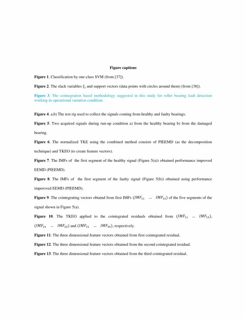
Figure captions
Figure 1. Classification by one-class SVM (from [37]).
Figure 2. The slack variables 行沈 and support vectors (data points with circles around them) (from [38]).
Figure 3. The cointegration based methodology suggested in this study for roller bearing fault detection
working in operational variation condition.
Figure 4. a,b) The test rig used to collect the signals coming from healthy and faulty bearings.
Figure 5. Two acquired signals during run-up condition a) from the healthy bearing b) from the damaged
bearing.
Figure 6. The normalized TKE using the combined method consists of PIEEMD (as the decomposition
technique) and TKEO (to create feature vectors).
Figure 7. The IMFs of the first segment of the healthy signal (Figure 5(a)) obtained performance improved
EEMD (PIEEMD).
Figure 8. The IMFs of the first segment of the faulty signal (Figure 5(b)) obtained using performance
imperoved EEMD (PIEEMD).
Figure 9. The cointegrating vectors obtaind from first IMFs 岫荊警繋怠怠 ┼ 荊警繋怠泰岻 of the five segments of the
signal shown in Figure 5(a).
Figure 10. The TKEO applied to the cointegrated residuals obtained from 岫荊警繋怠怠 ┼ 荊警繋怠泰岻, 岫荊警繋態怠 ┼ 荊警繋態泰岻 and 岫荊警繋戴怠 ┼ 荊警繋戴泰岻, respectively.
Figure 11. The three dimensional feature vectors obtained from first cointegrated residual.
Figure 12. The three dimensional feature vectors obtained from the second cointegrated residual.
Figure 13. The three dimensional feature vectors obtained from the third cointegrated residual.

Figure 14. The three dimensional feature vectors obtained from the fourth cointegrated residual.
Table captions
Table 1. The results of cointegration for the first IMFs of five segments of the healthy signal shown in Figure
5(a)
Table 2. The classification results for different cointegrated residuals
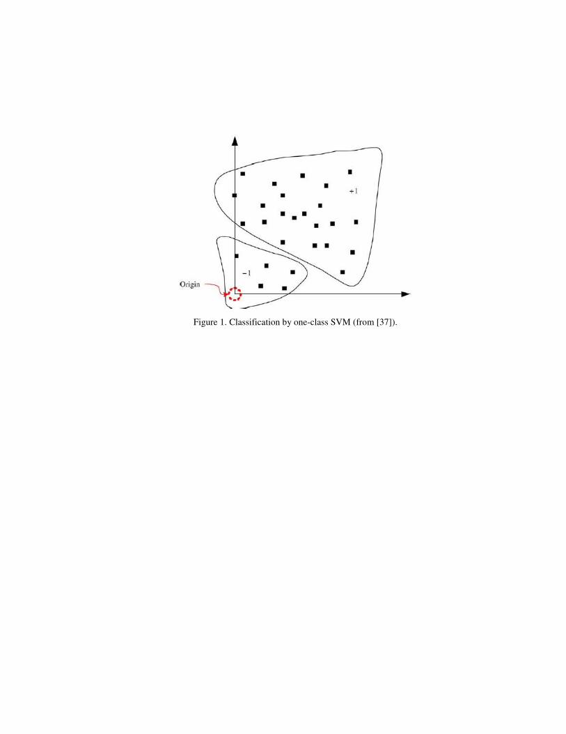
Figure 1. Classification by one-class SVM (from [37]).
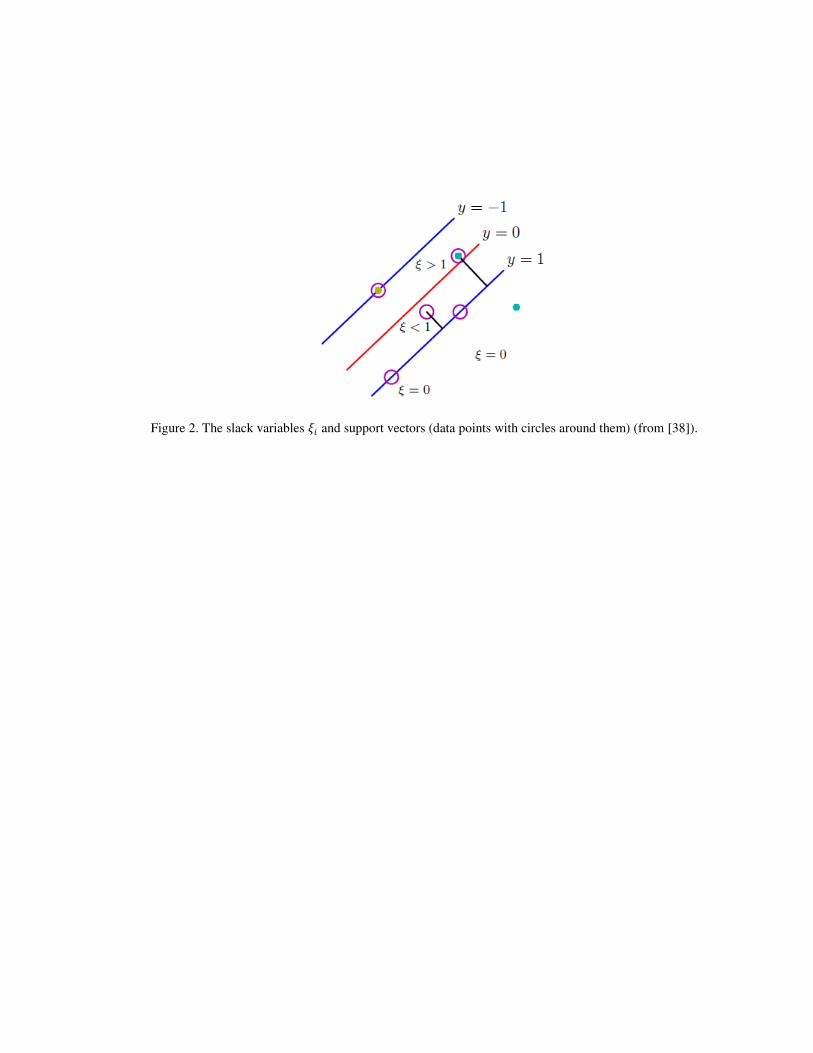
Figure 2. The slack variables 行件 and support vectors (data points with circles around them) (from [38]).
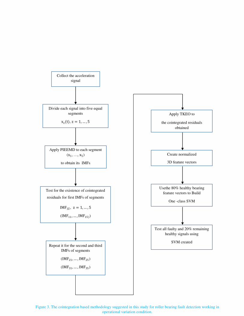
Figure 3. The cointegration based methodology suggested in this study for roller bearing fault detection working in
operational variation condition.
Collect the acceleration
signal
Divide each signal into five equal
segments
xz(t), z = 1, ┼ , 5
Apply PIEEMD to each segment
(x1, …, x5)
to obtain its IMFs
Test for the existence of cointegrated
residuals for first IMFs of segments
IMF1Z , z = 1, ┼ , 5
(IMF11 , ┼ , IMF15))
Apply TKEO to
the cointegrated residuals
obtained
Create normalized
3D feature vectors
Usethe 80% healthy bearing
feature vectors to Build
One -class SVM
Test all faulty and 20% remaining
healthy signals using
SVM created Repeat it for the second and third
IMFs of segments
(IMF21 , ┼ , IMF25)
(IMF31 , ┼ , IMF35)
(a)
(b)
Figure 4. a,b) The test rig used to collect the signals coming from healthy and faulty bearings.
a)
b)
Figure 5. Two acquired signals during run-up condition a) from the healthy bearing b) from the damaged bearing.
0 5 10 15 20 25-2
-1.5
-1
-0.5
0
0.5
1
1.5
2
time (s)
0 5 10 15 20 25-2
-1.5
-1
-0.5
0
0.5
1
1.5
2
time (s)
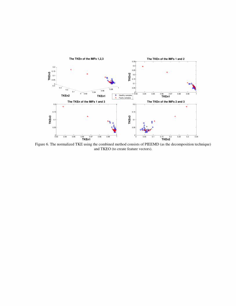
Figure 6. The normalized TKE using the combined method consists of PIEEMD (as the decomposition technique)
and TKEO (to create feature vectors).
0.920.94
0.960.98
1
00.1
0.20.3
0.40
0.05
0.1
0.15
0.2
TKEn1
The TKEn of the IMFs 1,2,3
TKEn2
TK
En
3
Healthy samples
Faulty samples
0.93 0.94 0.95 0.96 0.97 0.98 0.99 10
0.05
0.1
0.15
0.2
0.25
0.3
0.35
The TKEn of the IMFs 1 and 2
TKEn1
TK
En
2
0.93 0.94 0.95 0.96 0.97 0.98 0.99 10
0.05
0.1
0.15
0.2
The TKEn of the IMFs 1 and 3
TKEn1
TK
En
3
0 0.05 0.1 0.15 0.2 0.25 0.3 0.350
0.05
0.1
0.15
0.2
The TKEn of the IMFs 2 and 3
TKEn2
TK
En
3
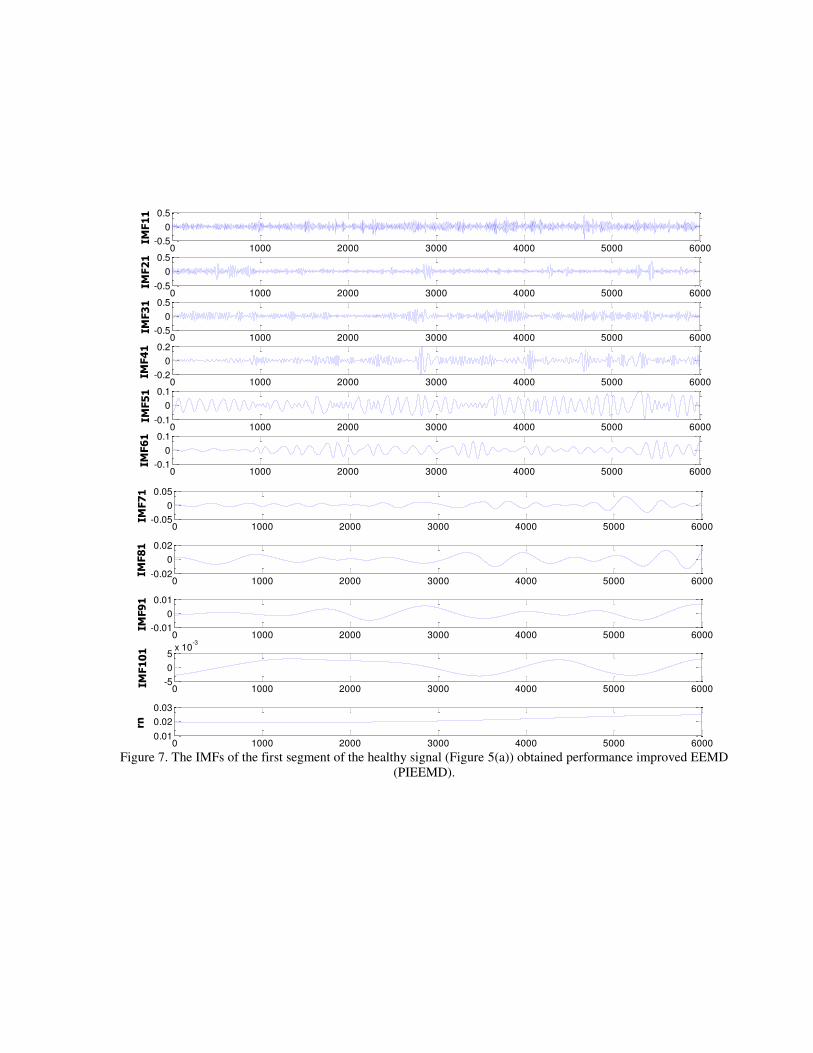
Figure 7. The IMFs of the first segment of the healthy signal (Figure 5(a)) obtained performance improved EEMD
(PIEEMD).
0 1000 2000 3000 4000 5000 6000-0.5
0
0.5
IMF11
0 1000 2000 3000 4000 5000 6000-0.5
0
0.5
IMF21
0 1000 2000 3000 4000 5000 6000-0.5
0
0.5
IMF31
0 1000 2000 3000 4000 5000 6000-0.2
0
0.2
IMF41
0 1000 2000 3000 4000 5000 6000-0.1
0
0.1
IMF51
0 1000 2000 3000 4000 5000 6000-0.1
0
0.1
IMF61
0 1000 2000 3000 4000 5000 6000-0.05
0
0.05
IMF71
0 1000 2000 3000 4000 5000 6000-0.02
0
0.02
IMF81
0 1000 2000 3000 4000 5000 6000-0.01
0
0.01
IMF91
0 1000 2000 3000 4000 5000 6000-5
0
5x 10
-3
IMF101
0 1000 2000 3000 4000 5000 60000.01
0.02
0.03
rn
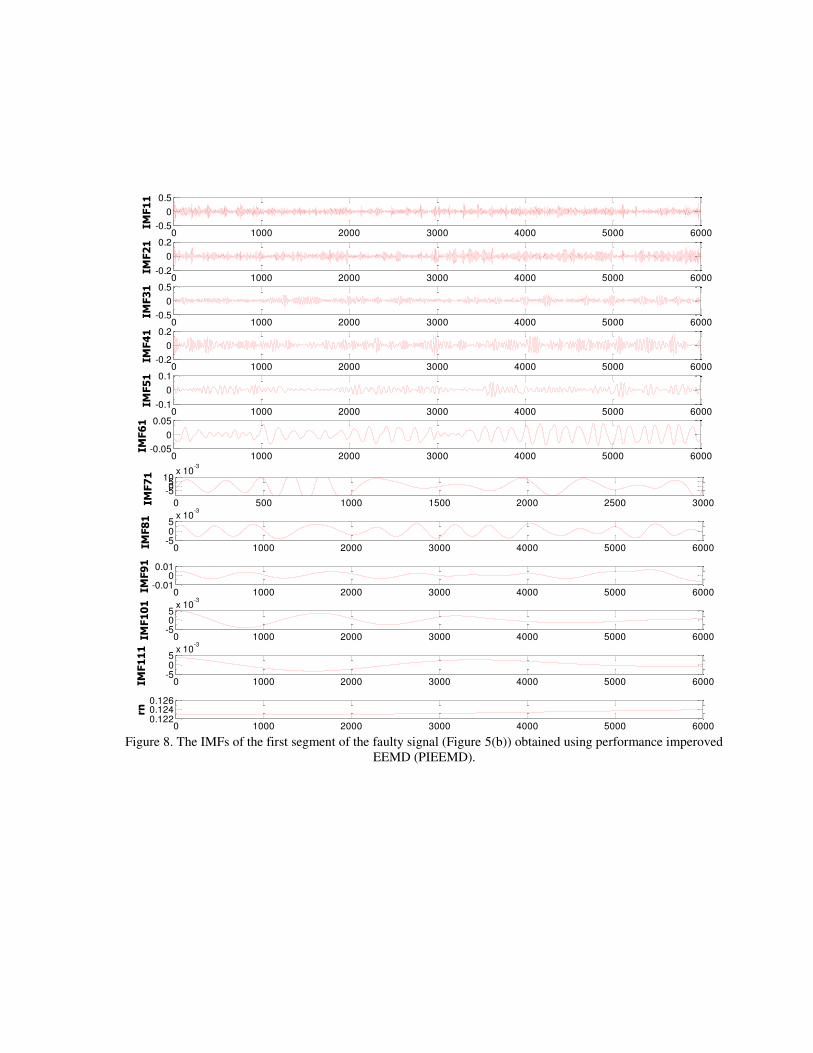
Figure 8. The IMFs of the first segment of the faulty signal (Figure 5(b)) obtained using performance imperoved
EEMD (PIEEMD).
0 1000 2000 3000 4000 5000 6000-0.5
0
0.5
IMF11
0 1000 2000 3000 4000 5000 6000-0.2
0
0.2
IMF21
0 1000 2000 3000 4000 5000 6000-0.5
0
0.5
IMF31
0 1000 2000 3000 4000 5000 6000-0.2
0
0.2
IMF41
0 1000 2000 3000 4000 5000 6000-0.1
0
0.1
IMF51
0 1000 2000 3000 4000 5000 6000-0.05
0
0.05
IMF61
0 500 1000 1500 2000 2500 3000
-50510
x 10-3
IMF71
0 1000 2000 3000 4000 5000 6000-505
x 10-3
IMF81
0 1000 2000 3000 4000 5000 6000-0.01
00.01
IMF91
0 1000 2000 3000 4000 5000 6000-505
x 10-3
IMF101
0 1000 2000 3000 4000 5000 6000-505
x 10-3
IMF111
0 1000 2000 3000 4000 5000 60000.1220.1240.126
rn
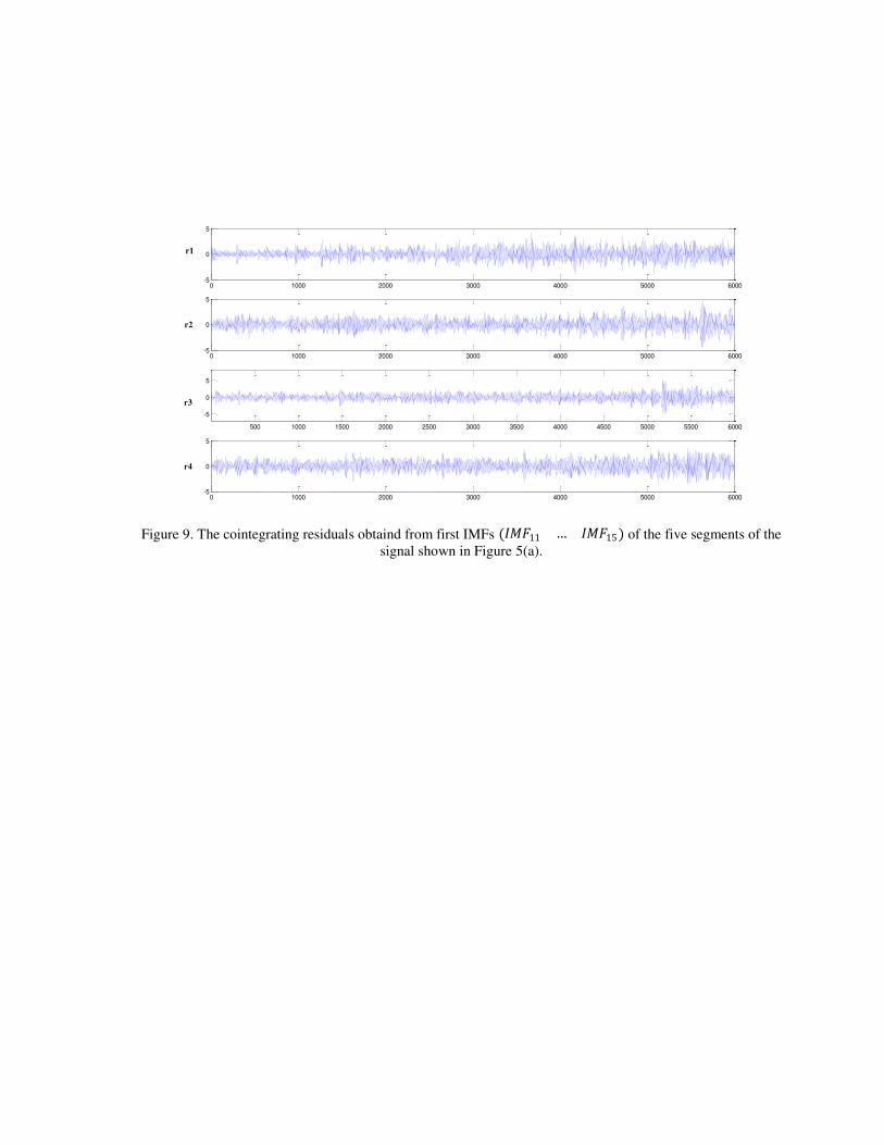
Figure 9. The cointegrating residuals obtaind from first IMFs 岫荊警繋11 ┼ 荊警繋15 岻 of the five segments of the
signal shown in Figure 5(a).
0 1000 2000 3000 4000 5000 6000-5
0
5
0 1000 2000 3000 4000 5000 6000-5
0
5
500 1000 1500 2000 2500 3000 3500 4000 4500 5000 5500 6000
-5
0
5
0 1000 2000 3000 4000 5000 6000-5
0
5
r4
r3
r2
r1
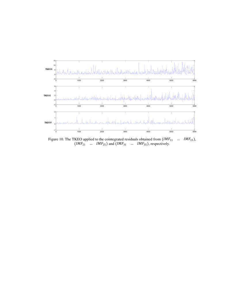
Figure 10. The TKEO applied to the cointegrated residuals obtained from 岫荊警繋11 ┼ 荊警繋15岻, 岫荊警繋21 ┼ 荊警繋25岻 and 岫荊警繋31 ┼ 荊警繋35岻, respectively.
0 1000 2000 3000 4000 5000 6000-5
0
5
10
15
0 1000 2000 3000 4000 5000 6000-2
0
2
4
6
0 1000 2000 3000 4000 5000 6000-1
0
1
2
TKEO1
TKEO2
TKEO3
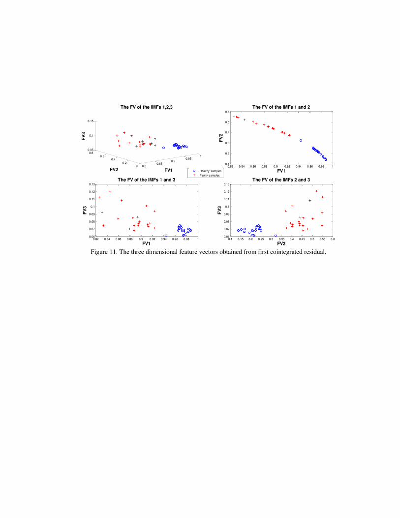
Figure 11. The three dimensional feature vectors obtained from first cointegrated residual.
0.80.85
0.90.95
1
00.2
0.40.6
0.80.05
0.1
0.15
FV1
The FV of the IMFs 1,2,3
FV2
FV
3
Healthy samples
Faulty samples
0.82 0.84 0.86 0.88 0.9 0.92 0.94 0.96 0.98 10.1
0.2
0.3
0.4
0.5
0.6
The FV of the IMFs 1 and 2
FV1
FV
2
0.82 0.84 0.86 0.88 0.9 0.92 0.94 0.96 0.98 10.06
0.07
0.08
0.09
0.1
0.11
0.12
0.13
The FV of the IMFs 1 and 3
FV1
FV
3
0.1 0.15 0.2 0.25 0.3 0.35 0.4 0.45 0.5 0.55 0.60.06
0.07
0.08
0.09
0.1
0.11
0.12
0.13
The FV of the IMFs 2 and 3
FV2
FV
3

Figure 12. The three dimensional feature vectors obtained from the second cointegrated residual.
0.750.8
0.850.9
0.951
00.2
0.40.6
0.80.05
0.1
0.15
FV1
The FV of the IMFs 1,2,3
FV2
FV
3
Healthy samples
Faulty samples
0.75 0.8 0.85 0.9 0.95 10.1
0.2
0.3
0.4
0.5
0.6
0.7
0.8
The FV of the IMFs 1 and 2
FV1
FV
2
0.75 0.8 0.85 0.9 0.95 10.06
0.08
0.1
0.12
0.14
0.16
The FV of the IMFs 1 and 3
FV1
FV
3
0.2 0.25 0.3 0.35 0.4 0.45 0.5 0.55 0.6 0.650.06
0.08
0.1
0.12
0.14
0.16
The FV of the IMFs 2 and 3
FV2
FV
3
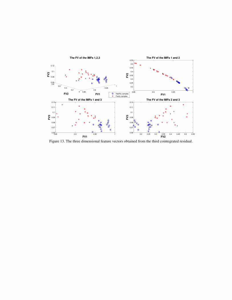
Figure 13. The three dimensional feature vectors obtained from the third cointegrated residual.
0.850.9
0.951
00.2
0.40.6
0.80.06
0.08
0.1
0.12
FV1
The FV of the IMFs 1,2,3
FV2
FV
3
Healthy samples
Faulty samples
0.85 0.9 0.95 1
0.2
0.25
0.3
0.35
0.4
0.45
0.5
0.55
The FV of the IMFs 1 and 2
FV1
FV
2
0.85 0.9 0.95 10.06
0.07
0.08
0.09
0.1
0.11
0.12
The FV of the IMFs 1 and 3
FV1
FV
3
0.2 0.25 0.3 0.35 0.4 0.45 0.5 0.550.06
0.07
0.08
0.09
0.1
0.11
0.12
The FV of the IMFs 2 and 3
FV2
FV
3

Figure 14. The three dimensional feature vectors obtained from the fourth cointegrated residual.
0.90.92
0.940.96
0.981
0.10.2
0.30.4
0.50.04
0.06
0.08
0.1
0.12
FV1
The FV of the IMFs 1,2,3
FV2
FV
3
Healthy samples
Faulty samples
0.9 0.91 0.92 0.93 0.94 0.95 0.96 0.97 0.98 0.990.1
0.15
0.2
0.25
0.3
0.35
0.4
0.45
0.5
The FV of the IMFs 1 and 2
FV1
FV
2
0.9 0.91 0.92 0.93 0.94 0.95 0.96 0.97 0.98 0.990.04
0.05
0.06
0.07
0.08
0.09
0.1
0.11
The FV of the IMFs 1 and 3
FV1
FV
3
0.1 0.15 0.2 0.25 0.3 0.35 0.4 0.45 0.50.04
0.05
0.06
0.07
0.08
0.09
0.1
0.11
The FV of the IMFs 2 and 3
FV2
FV
3
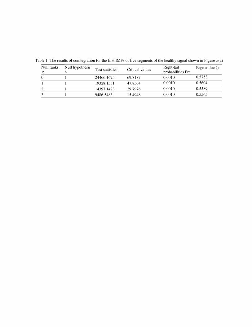
Table 1. The results of cointegration for the first IMFs of five segments of the healthy signal shown in Figure 5(a)
Null ranks
r
Null hypothesis
h Test statistics Critical values
Right-tail
probabilities Prt Eigenvalue r
0 1 24466.1675 69.8187 0.0010 0.5753
1 1 19328.1531 47.8564 0.0010 0.5604
2 1 14397.1423 29.7976 0.0010 0.5589
3 1 9486.5483 15.4948 0.0010 0.5565

Table 2. The classification results for different cointegrated residuals
Cointegrating
vectors training test Success ratio Margin
1 100 100 24/24 1.00428
2 100 100 24/24 1.00272
3 100 91.7 22/24 0.998041
4 100 83.3 20/24 0.999554


