
D. Chateigner, L. LutterottiNormandie Université, IUT-Caen,
Université de Caen NormandieCRISMAT-ENSICAEN
Universita Trento
Strain-Stress and Texture Combined Analysis
GFAC, Toulouse, 17-18th Nov. 2016
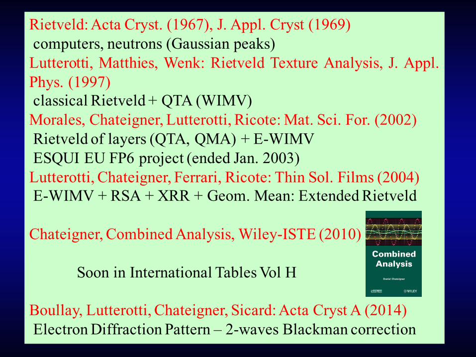
Rietveld: Acta Cryst. (1967), J. Appl. Cryst (1969)computers, neutrons (Gaussian peaks)Lutterotti, Matthies, Wenk: Rietveld Texture Analysis, J. Appl.Phys. (1997)classical Rietveld + QTA (WIMV)Morales, Chateigner, Lutterotti, Ricote: Mat. Sci. For. (2002)Rietveld of layers (QTA, QMA) + E-WIMVESQUI EU FP6 project (ended Jan. 2003)Lutterotti, Chateigner, Ferrari, Ricote: Thin Sol. Films (2004)E-WIMV + RSA + XRR + Geom. Mean: Extended Rietveld
Chateigner, Combined Analysis, Wiley-ISTE (2010)
Soon in International Tables Vol H
Boullay, Lutterotti, Chateigner, Sicard: Acta Cryst A (2014)Electron Diffraction Pattern – 2-waves Blackman correction

Structure|Fh|2Φ,L
Texturef(g)Φ,L
Residual Stress<Cijkl(g)>Φ,L
Real Layered samplesthicknessesroughnessesρ(z)… Phase
SΦ,L
defects (0D .. nD)broadeningasymmetry
Problematic

∫ϕ
ϕϕ=~
Sh~d)~,g(f)(P y
Rietveld: extended to lots of spectra∑∑ ∑= =Φ
ΦΦΦΦΦΦ
ΦΦ
ηθηθηθΩθν
+ηθ=ηθLN
1i
N
1ihh
2hh
h2c
i0bc ),,(A),,(P),,(Fj)(Lp
VI),,(y),,(y SSSSS yyyyy
Texture: E-WIMV, components, Harmonics, Exp. Harmonics …
Strain-Stress: ( ) geogeo1
N
1m
1m
N
1mm
1N
1mm
1geo CSSSSS m
mm ====⎥⎥⎦
⎤
⎢⎢⎣
⎡= −
=
ν−
=
ν−−
=
ν− ∏∏∏
Geometric mean, Voigt, Reuss, Hill …
Layering:AiΦ =
ν iΦ sinθi sinθoµ i (sinθi + sinθo )
1− e−µ iτ iW{ } e−µkτ kWk<i∏
W =1
sinθi+
1sinθo
Stacks, coatings,multilayers …

Popa, Delft: Crystallite sizes, shapes, microstrains, distributions
<Rh> = R0 + R1P20(x) + R2P2
1(x)cosϕ + R3P21(x)sinϕ + R4P2
2(x)cos2ϕ + R5P22(x)sin2ϕ +
...<εh2>Eh4 = E1h4 + E2k4 + E3!4 + 2E4h2k2 + 2E5!2k2 + 2E6h2!2 + 4E7h3k + 4E8h3! + 4E9k3h +
4E10k3! + 4E11!3h + 4E12!3k + 4E13h2k! + 4E14k2h! + 4E15!2kh
Line Broadening:
X-Ray Reflectivity (specular): Matrix, Parrat, DWBA, EDP …
X-Ray Fluorescence/GiXRF: De Boer
Electron Diffraction Patterns: 2-waves Blackman
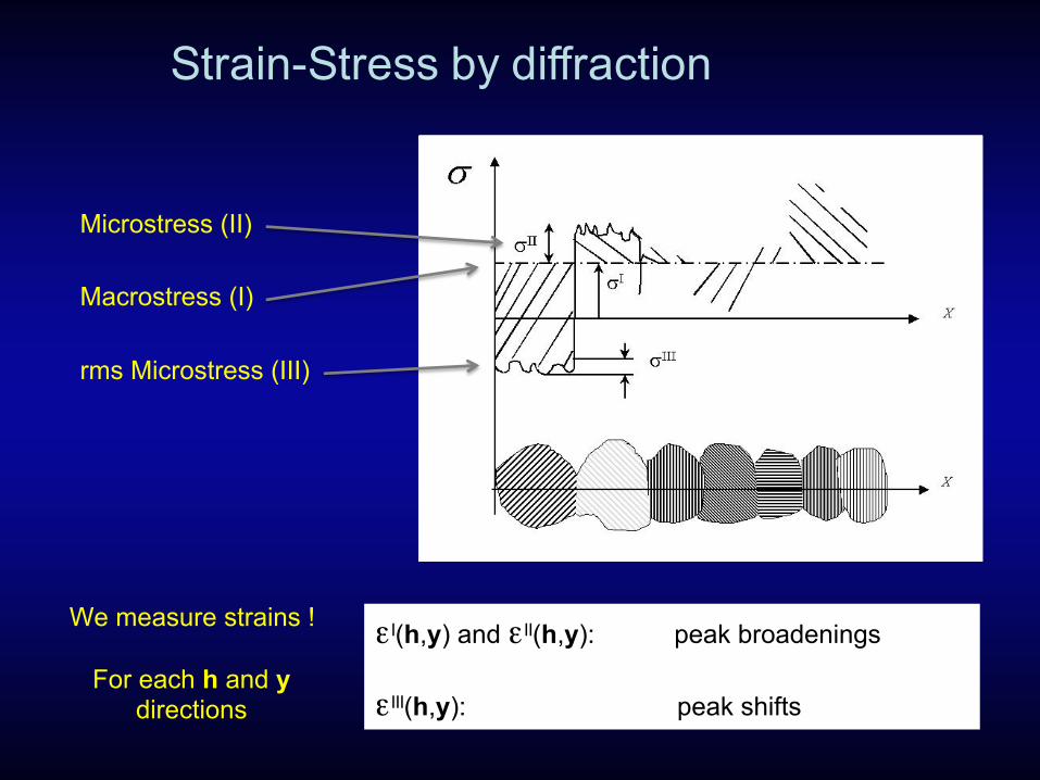
Strain-Stress by diffraction
Macrostress (I)
Microstress (II)
rms Microstress (III)
εI(h,y) and εII(h,y): peak broadenings
εIII(h,y): peak shifts
We measure strains !
For each h and ydirections

For non-textured (isotropic) samples
ε I (h, y) = 1+νE
σφ −σ 33( )sin2ψ + σ13 cosφ +σ 23 sinφ( )sin2ψ⎡⎣ ⎤⎦−νEσ ii
=dh (ϕ,ψ) Vd
− dh,0dh,0
σ ii =σ11 +σ 22 +σ 33
σφ =σ11 cos2ϕ +σ12 sin2ϕ +σ 22 sin
2ϕ −σ 33
Triaxial state
Assuming σ33=0 and small penetration depth
ε I (h, y) = 1+νE
σφ sin2ψ −
νEσ11 +σ 22( ) linear sin2ψ law
But non-linear behaviour is observed: Textured (anisotropic) samples; anisotropicplasticity; thermal anisotropy …
Dolle (J. Appl. Cryst., 12, 489, 1979) analyzed the problem in general, then Noyan and Nguyen (plasticdeformation), Barral et al. (texture connection) …

For textured (anisotropic) samples
Arithmetic means:- Voigt model: εij is homogeneous, σkl not, upper bound for <Cijkl>- Reuss model: σij is homogeneous, εkl not, lower bound for <Cijkl>- Hill model: neither εij nor σkl are homogeneous, <Cijkl> “in between”
Inversion property is violated: <Cijkl> ≠ <Sijkl>-1
Geometric means: Inversion property is math property: <Cijkl> ≠ <Sijkl>-1
Scalar case (isotropic):
Egeo( )
−1
= e− νi lnEii=1
N
∑= e
νi lnEi−1
i=1
N
∑= E−1( )
geo

Geometric mean of elastic tensorsElastic tensors are diagonally symmetric, but not diagonal !: need todiagonalise them first: C(λ) with bij
(λ) eigentensors
Cijkℓ = C(λ )bij(λ )bkℓ
(λ )
λ=1
6
∑lnC( )ijkℓ
= ln(C(λ ) )bij(λ )bkℓ
(λ )
λ=1
6
∑
= ln (C(λ ) )bij(λ )bkℓ
(λ )
λ=1
6
∏⎡
⎣⎢
⎤
⎦⎥
CijklMacro =Cijkl
geo= elnCi ' j 'k 'l ' = e Θ ijkℓ,i'j'k'ℓ' lnC( )i ' j 'k 'l '
Θijkℓ,i'j'k'ℓ'
= Θii' (g)Θ j
j' (g)Θkk' (g)Θℓ
ℓ' (g) f(g) dgg∫
Which are weighted over orientations:
Satisfying Hooke’s law Cijk!M = (Cijk!
-1,M)-1σij,M = Cijk!M εk!
M with

Multiphase sampleFor simplicity, take the isotropic case (N phases φn with phase fractionsνn):
EM = νnEnn=1
N
∑Voigt: EM ≠ EM−1( )
−1and
EM−1 = νnEn
−1
n=1
N
∑Reuss: EM−1 ≠ EM( )
−1and
lnEM = νn lnEnn=1
N
∑Geo:
EM = EM−1( )
−1andEM = e
νn lnEnn=1
N
∑
Matthies et Humbert (J. Appl. Cryst. 1995) for single phase, Matthies (Sol. Stat. Phen. 2010)

f n+1(g) = f n (g) h=1
I
∏m=1
Mh
∏ Phexp (y)
h=1
I
∏m=1
Mh
∏ Phn (y)
⎛
⎝
⎜⎜⎜⎜
⎞
⎠
⎟⎟⎟⎟
whrnIMh
E-WIMV (Rietveld only):
with 0 < rn < 1, relaxation parameter,Mh number of division points of the integralaround k,wh reflection weight
Orientation Distribution in Rietveld
f(g) is always positive (<> harmonics)Ghost conditional correctionsWorks for complex and sharp texturesAll symmetries (texture and crystal) down to triclinic

Extracted Intensities
Orientation Distribution Function
Residual stressesStrain Distribution Function
Structure+
Microstructure+
phase %
Popa-Balzar, sin2ψ
Structural parametersatomic positions, substitutions, vibrations
cell parameters
Multiphased, layered samples:Thickness,
Anisotropic Sizesand µ−strains (Popa),
Stacking faults (Warren),Distributions, Turbostratism (Ufer)
Phase ratio (amorphous + crystalline)Le Bail Rietveld
SAXS: X-Ray specular Reflectivity
Roughness, electron Density
& EDP,Thickness
Le Bail
Fresnel,Matrix (Parrat),
DWBA
WIMV, E-WIMVHarmonics, components, ADC
Rietveld
Combined Analysis approach
Voigt, Reuss,
Geometric mean
pole figuresinverse pole figures
TEM, XRF, PDF, EDX

WSS = ut wit yitc − yito( )2i=0
Nt
∑t=1
Np
∑
Combined Analysis cost function
For each pattern t: wit : weight, usually 1/yi = σ2.
ut : weight of each pattern tshould be used to adjust the importance we want to give to a particular technique or pattern with respect to the others

Minimum experimentalrequirements
1D or 2D Detector + 4-circle diffractometer
(CRISMAT – ANR EcoCorail)
~1000 experiments (2θ diagrams) Instrument calibrationin as many sample orientations + (peaks widths and shapes,
misalignments, defocusing …)

Mg0.75Fe0.25O high pressure experiments
E-WIMV + geo
a = 3.98639(3) Å<t> = 46.8(3) Å<ε> = 0.00535(1)σ33 = -861(3) MPa

Zr0.8Ca0.2O2 film orthorhombic texture
a = 5.146(2) Å<t> = 106(2) Å<ε> = 0.00333(5)σ11 = σ22 -2.62(8) GPa
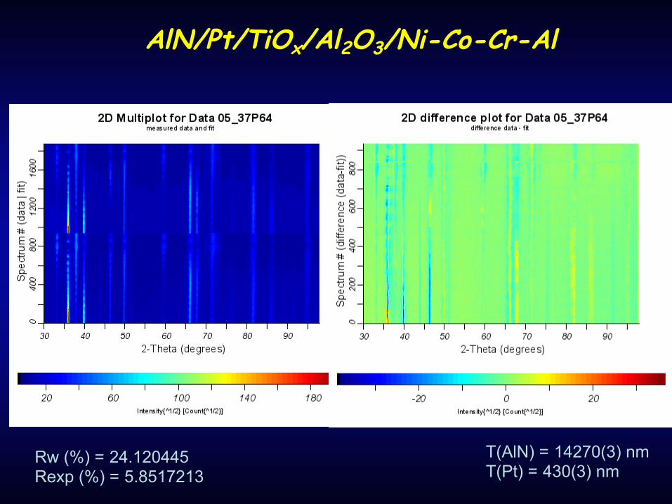
AlN/Pt/TiOx/Al2O3/Ni-Co-Cr-Al
Rw (%) = 24.120445Rexp (%) = 5.8517213
T(AlN) = 14270(3) nmT(Pt) = 430(3) nm

(χ,ϕ) randomly selected diagrams
Ni,Coa = 3.569377(5) Å<t> = 7600(1900) Å<ε> = 0.00236(3)σ11 = -328(8) MPaσ22 = -411(9) MPa
Al2O3
a = 4.7562(6) Åc = 12.875(3) ÅT= 7790(31) nm<t> = 150(2) Å<ε> = 0.008(3)

Rw (%) = 4.1
a = 3.11203(1) Åc = 4.98252(1) ÅT = 14270(3) nm<t> = 2404(8) Å<ε> = 0.001853(2)σ11 = -1019(2) MPaσ22 = -845(2) MPa
Rw (%) = 33.3
a = 3.91198(1) ÅT = 1204(3) nm<t> = 2173(10) Å<ε> = 0.002410(3)σ11 = -196.5(8)σ22 = -99.6(6)
AlN
Pt
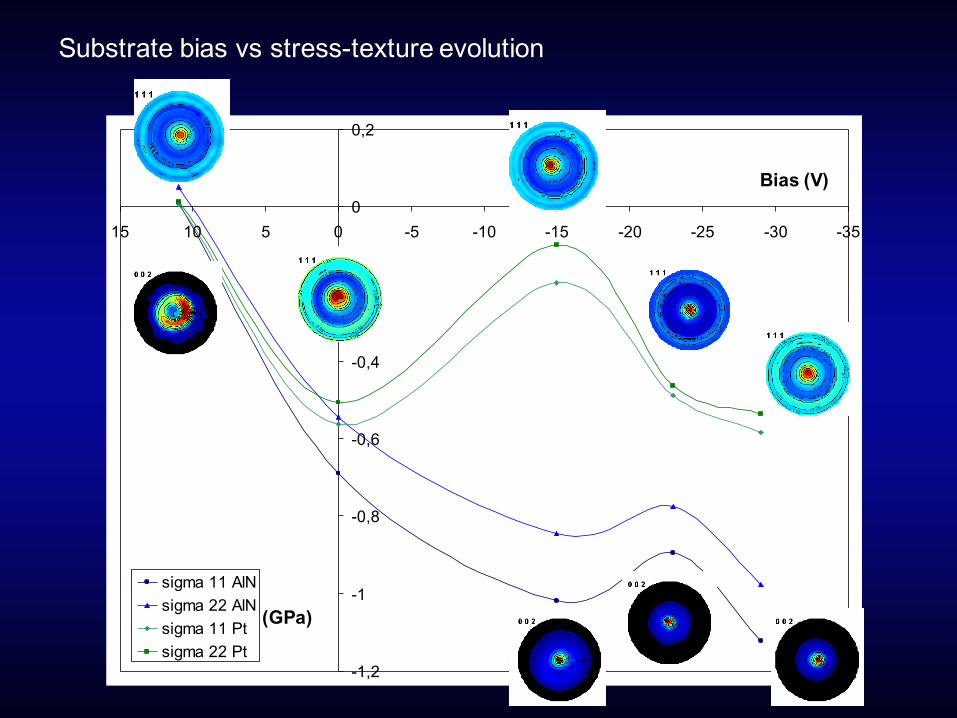
-1,2
-1
-0,8
-0,6
-0,4
-0,2
0
0,2
-35-30-25-20-15-10-5051015
sigma 11 AlNsigma 22 AlNsigma 11 Ptsigma 22 Pt
Substrate bias vs stress-texture evolution
(GPa)
Bias (V)

Si wafer
401.95 Å In2O3
401.87 Å In2O3
58.85 Å Ag
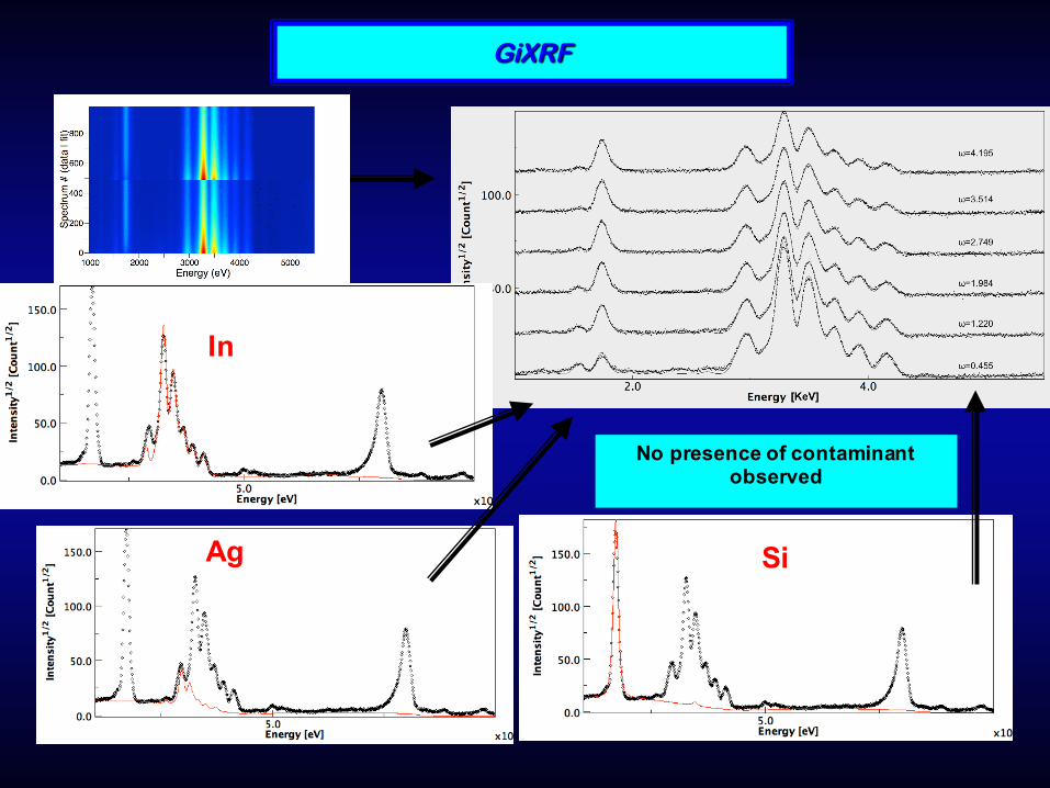
GIXRF
XRD
stress
Combinedanalysis
XRR
Combined XRR, XRD & GiXRF Analysis

XRR
Si wafer
400 Å In2O3
400 Å In2O3
60 Å Ag
Top layer: qc = 0.0294 Å-1; roughness r =0.38nmTop In2O3: qc = 0.0504 Å-1; r =2.06 nmAg : qc = 0.0576 Å-1; r =0.26 nmBottom In2O3: qc = 0.04889 Å-1; r =6.74 nmSi wafer: qc = 0.0313 Å-1; r = 0.73 nm
Highly porous In2O3 layer
Rw (%) = 4.05Rwnb (%, no bkg) = 4.56
Rb (%) = 3.44Rexp (%) = 4.15
Si wafer
403.1 Å In2O3
384.9 Å In2O3
57.4 Å Ag
17.9 Å In2O3 porous
Parrat formalism
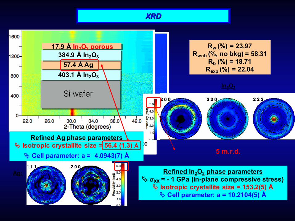
In2O3
XRD
Refined In2O3 phase parametersÄ σXX = - 1 GPa (in-plane compressive stress)
Ä Isotropic crystallite size = 153.2(5) ÅÄ Cell parameter: a = 10.2104(5) Å
Rw (%) = 23.97Rwnb (%, no bkg) = 58.31
Rb (%) = 18.71Rexp (%) = 22.04
5 m.r.d.
Refined Ag phase parametersÄ Isotropic crystallite size = 56.4 (1.3) Å
Ä Cell parameter: a = 4.0943(7) Å
Si wafer
403.1 Å In2O3
384.9 Å In2O3
57.4 Å Ag
17.9 Å In2O3 porous
Ag:
In
Ag Si
GiXRF
No presence of contaminant observed

Why not more ?
electronsmuons
neutrons
photons(X, γ, IR …)
MAUD, JanaFullprof …
MagneticNuclear (isotopic) scatteringSANS, n-Tomography, PDF
StructureLocal environment
TextureResidual Stresses
PhasesThickness
RoughnessPorositySize and shapeAmorphization
CompositionInterfaces
NanoscalesMisorientations
DislocationsTwins, Faults
Macroscale Magnetic structure Magnetic Texture
Magnetic roughness Vacancies
Atomic scale
Open Databases
H!
ij,p σ
E!
T,T ∇!
µ!
νh
Combined Analysis Workshop in Caen:3-7th July 2017 !
www.ecole.ensicaen.fr/~chateign/formation/
Thanks to the Labex
to the EU via the European Project
and to the


