
Clustering

What is Clustering? Finding groups of objects such that objects in a group will be similar to
one another and different from the objects in other groups
A type of unsupervised learning and can be viewed as unsupervised segmentation (sometimes called classification by statisticians, sorting by psychologists, and segmentation by people in marketing
Inter-cluster distances are maximized
Intra-cluster distances are
minimized

3 School Employees Simpson's Family Males Females
Clustering is subjective
What is a natural grouping among these objects?

4
Similarity is Subjective

5
Intuitions behind desirable
distance measure properties
D(A,B) = D(B,A) Symmetry Otherwise you could claim “Alex looks like Bob, but Bob looks nothing like Alex.”
D(A,A) = 0 Constancy of Self-Similarity Otherwise you could claim “Alex looks more like Bob, than Bob does.”
D(A,B) = 0 if and only if A=B Positivity (Separation) Otherwise there are objects in your world that are different, but you cannot tell apart.
D(A,B) D(A,C) + D(B,C) Triangular Inequality Otherwise you could claim “Alex is very like Bob, and Alex is very like Carl, but Bob is very unlike Carl.”

Applications of Cluster Analysis
Understanding
Group related documents for browsing Business news articles about a particular stock
Group genes and proteins with similar functionality
Group stocks with similar price fluctuations
Group customers with similar buying habits
Group Whisky with similar flavors
Summarization
Reduce the size of large data sets
Reduce the number of attributes Cluster using a group of attributes and replace these attributes
with one attribute that is the cluster label

Clustering Precipitation in Australia
7

Notion of a Cluster can be Ambiguous
How many clusters?
Four Clusters Two Clusters
Six Clusters
So tell me how
many clusters do
you see?

Types of Clusterings
A clustering is a set of clusters
Partitional Clustering A division data objects into non-overlapping subsets (clusters) such
that each data object is in exactly one subset
Hierarchical clustering A set of nested clusters organized as a hierarchical tree

Partitional Clustering
Original Points A Partitional Clustering

Hierarchical Clustering
p4
p1 p3
p2
p4p1 p2 p3
Traditional Hierarchical Clustering Traditional Dendrogram
Simpsonian Dendrogram

Other Distinctions Between Clusterings
Exclusive versus non-exclusive In non-exclusive clusterings points may belong to multiple clusters
Can represent multiple classes or ‘border’ points
Fuzzy versus non-fuzzy In fuzzy clustering, a point belongs to every cluster with some weight
between 0 and 1
Weights must sum to 1
Probabilistic clustering has similar characteristics
Partial versus complete In some cases, we only want to cluster some of the data

Types of Clusters
Well-separated clusters
Center-based clusters (our main emphasis)
Contiguous clusters
Density-based clusters
Described by an Objective Function

Types of Clusters: Well-Separated
Well-Separated Clusters: A clustering where any point in a cluster is closer (or more similar)
to every other point in the cluster than to any point not in the cluster.
3 well-separated clusters

Types of Clusters: Center-Based
Center-based A cluster is a set of objects such that an object in a cluster is closer
(more similar) to the “center” of a cluster, than to the center of any other cluster
The center of a cluster is often a centroid, the average of all the points in the cluster (assuming numerical attributes), or a medoid, the most “representative” point of a cluster (used if there are categorical features)
4 center-based clusters
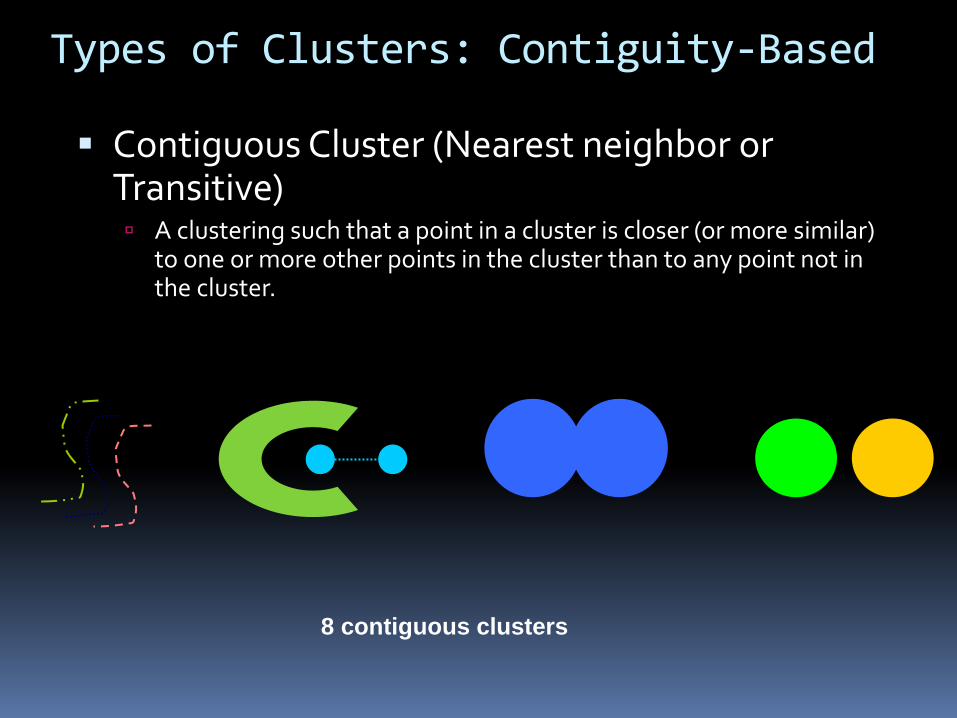
Types of Clusters: Contiguity-Based
Contiguous Cluster (Nearest neighbor or Transitive) A clustering such that a point in a cluster is closer (or more similar)
to one or more other points in the cluster than to any point not in the cluster.
8 contiguous clusters

Types of Clusters: Density-Based
Density-based A cluster is a dense region of points, which is separated by low-
density regions, from other regions of high density.
Used when the clusters are irregular or intertwined, and when noise and outliers are present.
6 density-based clusters

Types of Clusters: Objective Function
Clusters Defined by an Objective Function Finds clusters that minimize or maximize an objective
function.
Enumerate all possible ways of dividing the points into clusters and evaluate the `goodness' of each potential set of clusters by using the given objective function. (NP Hard)
Example: Sum of squares of distances to cluster center

Clustering Algorithms
K-means and its variants
Hierarchical clustering
Density-based clustering
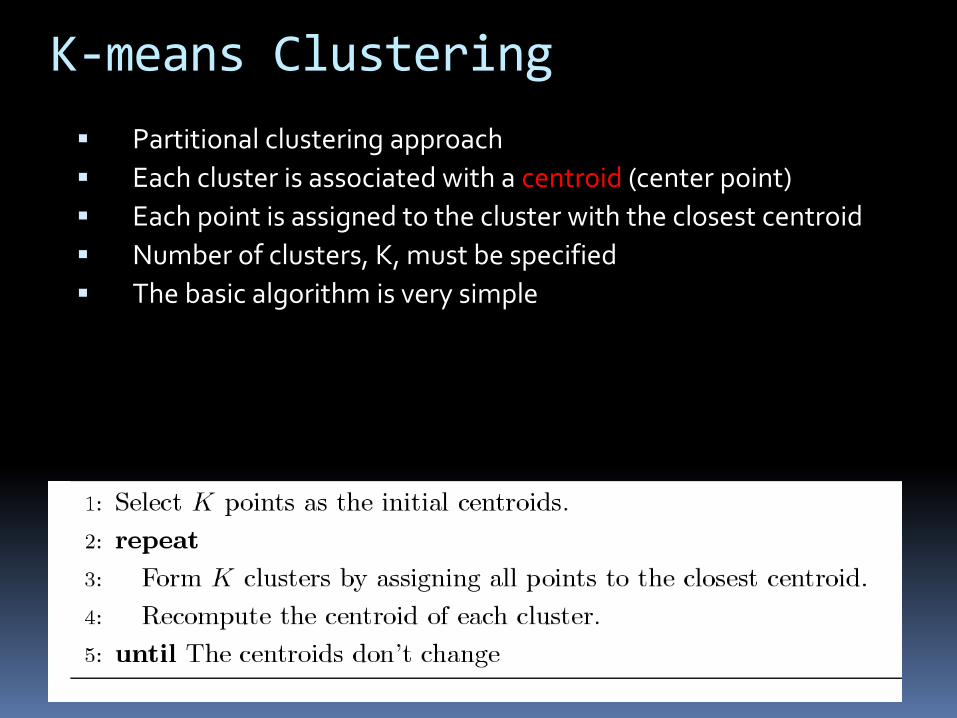
K-means Clustering
Partitional clustering approach
Each cluster is associated with a centroid (center point)
Each point is assigned to the cluster with the closest centroid
Number of clusters, K, must be specified
The basic algorithm is very simple
K-means Clustering
21
0
1
2
3
4
5
0 1 2 3 4 5
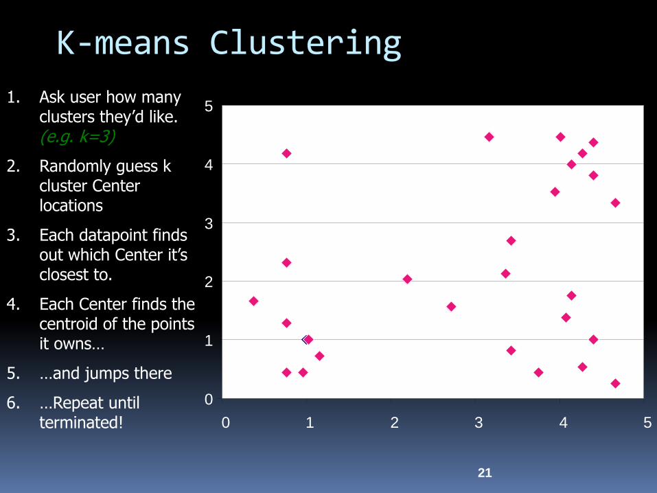
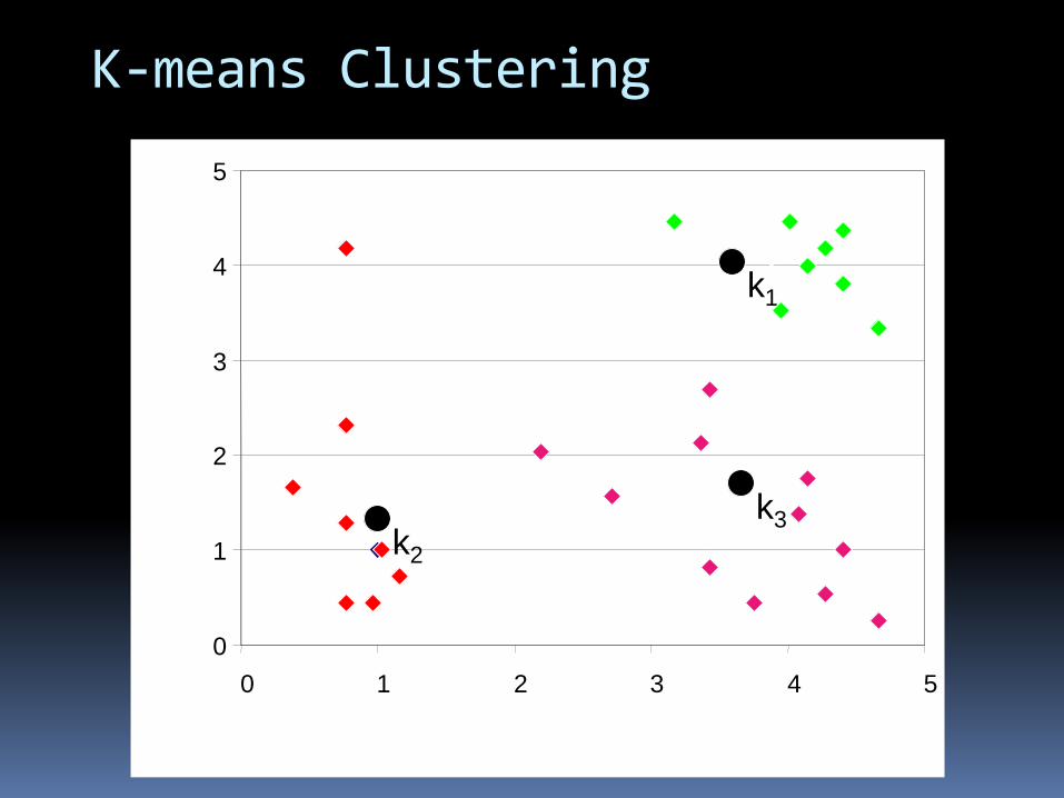
1. Ask user how many clusters they’d like. (e.g. k=3)
2. Randomly guess k cluster Center locations
3. Each datapoint finds out which Center it’s closest to.
4. Each Center finds the centroid of the points it owns…
5. …and jumps there
6. …Repeat until terminated!
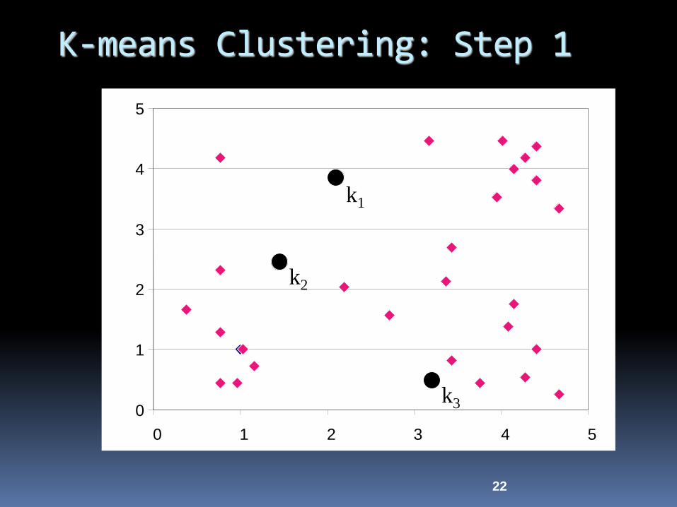
K-means Clustering: Step 1
22
0
1
2
3
4
5
0 1 2 3 4 5
k1
k2
k3

K-means Clustering
23
0
1
2
3
4
5
0 1 2 3 4 5
k1
k2
k3
K-means Clustering
24
0
1
2
3
4
5
0 1 2 3 4 5
k1
k2
k3

K-means Clustering
25
0
1
2
3
4
5
0 1 2 3 4 5
expression in condition 1
exp
ressio
n in
co
nd
itio
n 2
k1
k2 k3
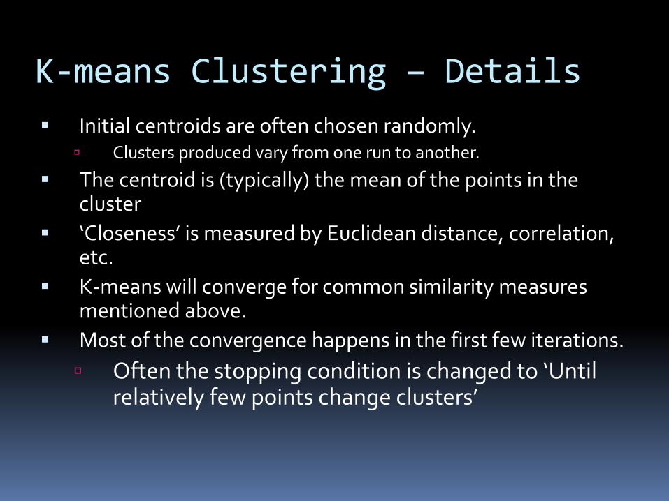
K-means Clustering – Details
Initial centroids are often chosen randomly. Clusters produced vary from one run to another.
The centroid is (typically) the mean of the points in the cluster
‘Closeness’ is measured by Euclidean distance, correlation, etc.
K-means will converge for common similarity measures mentioned above.
Most of the convergence happens in the first few iterations.
Often the stopping condition is changed to ‘Until relatively few points change clusters’

Evaluating K-means Clusters
Most common measure is Sum of Squared Error (SSE) For each point, the error is the distance to the nearest
cluster To get SSE, we square these errors and sum them. We can show that to minimize SSE the best update
strategy is to use the center of the cluster. Given two clusters, we can choose the one with the
smallest error One easy way to reduce SSE is to increase K, the
number of clusters A good clustering with smaller K can have a lower SSE
than a poor clustering with higher K

Two different K-means Clusterings
-2 -1.5 -1 -0.5 0 0.5 1 1.5 2
0
0.5
1
1.5
2
2.5
3
x
y
-2 -1.5 -1 -0.5 0 0.5 1 1.5 2
0
0.5
1
1.5
2
2.5
3
x
y
Sub-optimal Clustering
-2 -1.5 -1 -0.5 0 0.5 1 1.5 2
0
0.5
1
1.5
2
2.5
3
x
y
Optimal Clustering
Original Points

Importance of Choosing Initial Centroids
-2 -1.5 -1 -0.5 0 0.5 1 1.5 2
0
0.5
1
1.5
2
2.5
3
x
y
Iteration 1
-2 -1.5 -1 -0.5 0 0.5 1 1.5 2
0
0.5
1
1.5
2
2.5
3
x
y
Iteration 2
-2 -1.5 -1 -0.5 0 0.5 1 1.5 2
0
0.5
1
1.5
2
2.5
3
x
y
Iteration 3
-2 -1.5 -1 -0.5 0 0.5 1 1.5 2
0
0.5
1
1.5
2
2.5
3
x
y
Iteration 4
-2 -1.5 -1 -0.5 0 0.5 1 1.5 2
0
0.5
1
1.5
2
2.5
3
x
y
Iteration 5
-2 -1.5 -1 -0.5 0 0.5 1 1.5 2
0
0.5
1
1.5
2
2.5
3
x
y
Iteration 6
If you happen to choose good initial centroids, then you will
get this after 6 iterations

Importance of Choosing Initial Centroids
-2 -1.5 -1 -0.5 0 0.5 1 1.5 2
0
0.5
1
1.5
2
2.5
3
x
y
Iteration 1
-2 -1.5 -1 -0.5 0 0.5 1 1.5 2
0
0.5
1
1.5
2
2.5
3
x
y
Iteration 2
-2 -1.5 -1 -0.5 0 0.5 1 1.5 2
0
0.5
1
1.5
2
2.5
3
x
y
Iteration 3
-2 -1.5 -1 -0.5 0 0.5 1 1.5 2
0
0.5
1
1.5
2
2.5
3
x
y
Iteration 4
-2 -1.5 -1 -0.5 0 0.5 1 1.5 2
0
0.5
1
1.5
2
2.5
3
x
y
Iteration 5
-2 -1.5 -1 -0.5 0 0.5 1 1.5 2
0
0.5
1
1.5
2
2.5
3
x
y
Iteration 6
Good clustering

Importance of Choosing Initial Centroids …
-2 -1.5 -1 -0.5 0 0.5 1 1.5 2
0
0.5
1
1.5
2
2.5
3
x
y
Iteration 1
-2 -1.5 -1 -0.5 0 0.5 1 1.5 2
0
0.5
1
1.5
2
2.5
3
x
y
Iteration 2
-2 -1.5 -1 -0.5 0 0.5 1 1.5 2
0
0.5
1
1.5
2
2.5
3
x
y
Iteration 3
-2 -1.5 -1 -0.5 0 0.5 1 1.5 2
0
0.5
1
1.5
2
2.5
3
x
y
Iteration 4
-2 -1.5 -1 -0.5 0 0.5 1 1.5 2
0
0.5
1
1.5
2
2.5
3
xy
Iteration 5
Bad
Clustering

10 Clusters Example
0 5 10 15 20
-6
-4
-2
0
2
4
6
8
x
y
Iteration 1
0 5 10 15 20
-6
-4
-2
0
2
4
6
8
x
y
Iteration 2
0 5 10 15 20
-6
-4
-2
0
2
4
6
8
x
y
Iteration 3
0 5 10 15 20
-6
-4
-2
0
2
4
6
8
x
y
Iteration 4
Starting with two initial centroids in one cluster of each pair of clusters

10 Clusters Example
Starting with some pairs of clusters having three initial centroids, while other have only one.
0 5 10 15 20
-6
-4
-2
0
2
4
6
8
x
yIteration 1
0 5 10 15 20
-6
-4
-2
0
2
4
6
8
x
y
Iteration 2
0 5 10 15 20
-6
-4
-2
0
2
4
6
8
x
y
Iteration 3
0 5 10 15 20
-6
-4
-2
0
2
4
6
8
x
y
Iteration 4

Pre-processing and Post-processing
Pre-processing Normalize the data
Eliminate outliers
Post-processing Eliminate small clusters that may represent
outliers
Split ‘loose’ clusters, i.e., clusters with relatively high SSE
Merge clusters that are ‘close’ and that have relatively low SSE

Limitations of K-means
K-means has problems when clusters are of differing
Sizes (biased toward the larger clusters)
Densities
Non-globular shapes
K-means has problems when the data contains outliers.

Limitations of K-means:Differing Sizes
Original Points K-means (3 Clusters)

Limitations of K-means: Differing Density
Original Points K-means (3 Clusters)

Limitations of K-means: Non-globular Shapes
Original Points K-means (2 Clusters)

Overcoming K-means Limitations
Original Points K-means Clusters
One solution is to use many clusters.
Find parts of clusters, but need to put together.

Overcoming K-means Limitations
Original Points K-means Clusters

Hierarchical Clustering
Produces a set of nested clusters organized as a hierarchical tree
Can be visualized as a dendrogram
A tree like diagram that records the sequences of merges or splits
1 3 2 5 4 60
0.05
0.1
0.15
0.2
1
2
3
4
5
6
1
23 4
5

42 ANGUILLA AUSTRALIA St. Helena &
Dependencies
South Georgia &
South Sandwich
Islands U.K.
Serbia &
Montenegro
(Yugoslavia) FRANCE NIGER INDIA IRELAND BRAZIL
Hierarchal clustering can sometimes show
patterns that are meaningless or spurious • For example, in this clustering, the tight grouping of Australia, Anguilla,
St. Helena etc is meaningful, since all these countries are former UK
colonies.
• However the tight grouping of Niger and India is completely spurious,
there is no connection between the two.

43
We can look at the dendrogram to determine the “correct” number of clusters.
In this case, the two highly separated subtrees are highly suggestive of two
clusters. (Things are rarely this clear cut, unfortunately)

44
Outlier
One potential use of a dendrogram is to detect outliers
The single isolated branch is suggestive of a data
point that is very different to all others

45
Hierarchical Clustering
Build a tree-based hierarchical taxonomy (dendrogram) from a set of unlabeled examples.
Recursive application of a standard clustering algorithm can produce a hierarchical clustering.
animal
vertebrate
fish reptile amphib. mammal worm insect crustacean
invertebrate
Strengths of Hierarchical Clustering
Do not have to assume any particular number of clusters Any desired number of clusters can be obtained by
‘cutting’ the dendogram at the proper level
They may correspond to meaningful taxonomies Example in biological sciences (e.g., animal kingdom,
phylogeny reconstruction, …)

Hierarchical Clustering
Two main types of hierarchical clustering Agglomerative:
Start with the points as individual clusters
At each step, merge the closest pair of clusters until only one cluster (or k clusters) left
Divisive: Start with one, all-inclusive cluster
At each step, split a cluster until each cluster contains a point (or there are k clusters)
Agglomerative is most common

Starting Situation
...p1 p2 p3 p4 p9 p10 p11 p12
Start with clusters of individual points

Intermediate Situation
...p1 p2 p3 p4 p9 p10 p11 p12
After some merging steps, we have some clusters
C1
C4
C2 C5
C3

Intermediate Situation
...p1 p2 p3 p4 p9 p10 p11 p12
We want to merge the two closest clusters (C2 and C5)
C1
C4
C2 C5
C3

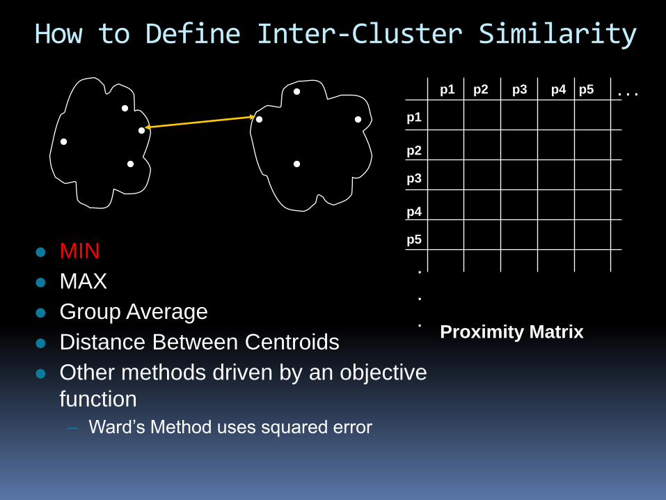
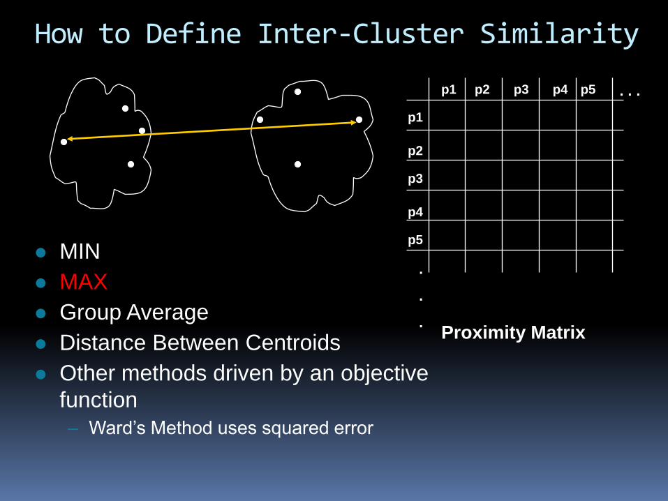
How to Define Inter-Cluster Similarity
p1
p3
p5
p4
p2
p1 p2 p3 p4 p5 . . .
.
.
.
Similarity?
MIN
MAX
Group Average
Distance Between Centroids
Other methods driven by an objective
function
– Ward’s Method uses squared error
Proximity Matrix
How to Define Inter-Cluster Similarity
p1
p3
p5
p4
p2
p1 p2 p3 p4 p5 . . .
.
.
. Proximity Matrix
MIN
MAX
Group Average
Distance Between Centroids
Other methods driven by an objective
function
– Ward’s Method uses squared error
How to Define Inter-Cluster Similarity
p1
p3
p5
p4
p2
p1 p2 p3 p4 p5 . . .
.
.
. Proximity Matrix
MIN
MAX
Group Average
Distance Between Centroids
Other methods driven by an objective
function
– Ward’s Method uses squared error

How to Define Inter-Cluster Similarity
p1
p3
p5
p4
p2
p1 p2 p3 p4 p5 . . .
.
.
. Proximity Matrix
MIN
MAX
Group Average
Distance Between Centroids
Other methods driven by an objective
function
– Ward’s Method uses squared error

How to Define Inter-Cluster Similarity
p1
p3
p5
p4
p2
p1 p2 p3 p4 p5 . . .
.
.
. Proximity Matrix
MIN
MAX
Group Average
Distance Between Centroids

Hierarchical Clustering: MIN
Nested Clusters Dendrogram
1
2
3
4
5
6
1
2
3
4
5
3 6 2 5 4 10
0.05
0.1
0.15
0.2

Hierarchical Clustering: MAX
Nested Clusters Dendrogram
3 6 4 1 2 50
0.05
0.1
0.15
0.2
0.25
0.3
0.35
0.4
1
2
3
4
5
6
1
2 5
3
4

Hierarchical Clustering: Problems and Limitations
Once a decision is made to combine two clusters, it cannot be undone
No objective function is directly minimized
Different schemes have problems with one or more of the following: Sensitivity to noise and outliers
Difficulty handling different sized clusters and convex shapes
Breaking large clusters

DBSCAN
DBSCAN is a density-based algorithm. Density = number of points within a specified radius (Eps)
A point is a core point if it has more than a specified number of
points (MinPts) within Eps
These are points that are at the interior of a cluster
A border point has fewer than MinPts within Eps, but is in the neighborhood of a core point
A noise point is any point that is not a core point or a border point.

DBSCAN: Core, Border, and Noise Points

DBSCAN: Core, Border and Noise Points
Original Points Point types: core,
border and noise
Eps = 10, MinPts = 4

When DBSCAN Works Well
Original Points Clusters
• Resistant to Noise
• Can handle clusters of different shapes and sizes

When DBSCAN Does NOT Work Well
Original Points
(MinPts=4, Eps=9.75).
(MinPts=4, Eps=9.92)
• Varying densities
Cluster Validity
For supervised classification we have a variety of measures to evaluate how good our model is Accuracy, precision, recall
For cluster analysis, the analogous question is how to evaluate the “goodness” of the resulting clusters?
But “clusters are in the eye of the beholder”!
Then why do we want to evaluate them? To avoid finding patterns in noise To compare clustering algorithms To compare two sets of clusters To compare two clusters

Clusters found in Random Data
0 0.2 0.4 0.6 0.8 10
0.1
0.2
0.3
0.4
0.5
0.6
0.7
0.8
0.9
1
x
y
Random
Points
0 0.2 0.4 0.6 0.8 10
0.1
0.2
0.3
0.4
0.5
0.6
0.7
0.8
0.9
1
x
y
K-means
0 0.2 0.4 0.6 0.8 10
0.1
0.2
0.3
0.4
0.5
0.6
0.7
0.8
0.9
1
x
y
DBSCAN

Internal Measures: SSE Clusters in more complicated figures aren’t well separated
Internal Index: Used to measure the goodness of a clustering structure without respect to external information
SSE
SSE is good for comparing two clusterings or two clusters (average SSE).
Can also be used to estimate the number of clusters
2 5 10 15 20 25 300
1
2
3
4
5
6
7
8
9
10
K
SS
E
5 10 15
-6
-4
-2
0
2
4
6

Internal Measures: SSE
SSE curve for a more complicated data set
1
2
3
5
6
4
7
SSE of clusters found using K-means

Final Comment on Cluster Validity
“The validation of clustering structures is the most difficult and frustrating part of cluster analysis.
Without a strong effort in this direction, cluster analysis will remain a black art accessible only to those true believers who have experience and great courage.”
Algorithms for Clustering Data, Jain and Dubes
Understanding the Clustering
How might you understand what the different clusters represent? The names/identifiers may indicate a pattern if they
are well known You can represent the clusters by a prototype
(centroid) and this can be insightful You can provide statistics (e.g., mean) to describe the
features of the objects in each cluster In a class many years ago we had a cluster that you could
name “Educated Single Women” based on the feature averages.
But it is not always easy to truly understand the clusters
69

Using Supervised Learning to Generate Cluster Descriptions
Supervised learning can help understand the clusters
Create a class variable that is assigned the cluster identifier
Then apply supervised learning using an interpretable classifier (rule-based or decision tree)
The classifier can help describe the cluster
70

Descriptive Data Mining
Clustering is a descriptive task
The problem/task that you are addressing may not be nearly as well defined as with a prediction task, where you must formulate a precise learning problem
Even if your task is to do market segmentation for a marketing campaign, it is not clear what to do with the clustering
You tend to have more work to do after the data mining phase
71

Clustering with WEKA
Run Weka Explorer and open the vote dataset that comes with WEKA
This is the “Congressional Voting Records” data set from the UCI Machine Learning Repository
Votes for each of the U.S. House of Representatives Congressmen on 16 key votes
The class is “democrat” or “republican”
Go to cluster tab and choose “SimpleKMeans”
Use default parameters, including N=2 clusters
72

Clustering Output for “Vote”
73
kMeans
======
Number of iterations: 3
Within cluster sum of squared errors: 1510.0
Missing values globally replaced with mean/mode
Cluster centroids:
Cluster#
Attribute Full Data 0 1
(435) (214) (221)
=========================================================================
handicapped-infants n n y
water-project-cost-sharing y y n
adoption-of-the-budget-resolution y n y
physician-fee-freeze n y n
el-salvador-aid y y n
religious-groups-in-schools y y n
anti-satellite-test-ban y n y
aid-to-nicaraguan-contras y n y
mx-missile y n y
immigration y y y
synfuels-corporation-cutback n n n
education-spending n y n
superfund-right-to-sue y y n
crime y y n
duty-free-exports n n y
export-admin-act-south-africa y y y
Class dem rep dem
When reran with N=4
clusters appeared to split
democrats into 3 groups
Cluster 1: 40% (rep)
Cluster 2: 12% (dem)
Cluster 3: 13% (dem)
Cluster 4: 35% (dem)


