IV-1
Chap ter
1 Perceptual Mapping
Leland Wilkinson
PERMAP offers two types of tools. The first is a group of procedures for fitting subjects and objects in a common space. This group includes Carroll’s (1972) internal and external unfolding models, MDPREF and PREFMAP, as well as Gabriel’s (1971) BIPLOT, which is a minor modification of MDPREF. The second is a set of procedures for relating one dimensional configuration to another, generally called a procrustes rotation. Both the orthogonal procrustes and the more general canonical rotations are available.
PERMAP is a misnomer. Although most of the techniques it incorporates have been used for perceptual mapping, they have applications outside of market research or psychology and, like the biplot technique, may even have their origins elsewhere. Furthermore, classical perceptual mapping techniques, such as multidimensional scaling, correspondence analysis, and principal components, are found elsewhere in SYSTAT. In the end, since almost all of the methods in this module involve a singular value decomposition and are not bulky enough to deserve their own modules, they have been collected into a single grab bag.
Statistical BackgroundPerceptual mapping involves a variety of techniques for displaying the judgments of a set of objects by a group of subjects. Most of these techniques were developed in the 1970’s by psychometricians, but they were soon adopted by market researchers and scientists for analyzing a variety of preference and similarity data.
In applied usage, especially among market researchers, perceptual mapping is an even more general term. Some commercial perceptual mapping programs are based

IV-2
Chapter 1
on classical statistical or psychometric models. Some of these methods include Fisher’s linear discriminant function, correspondence analysis, factor analysis, and multidimensional scaling. Indeed, any procedure that produces a set of coordinates in a q dimensional space from an matrix, , can be considered perceptual mapping in the broad, applied sense. Quantitative theoretical market researchers (for example, Green and Tull, 1975, and Lilien, Kotler, and Moorthy, 1992) use the term in this more general sense as well.
The origin of the term can be found in classical psychometrics (see Cliff, 1973, for a review). Soon after the development of psychometric spatial models, some psychologists thought scaling methods could be used to derive “cognitive maps” from the subject’s ratings of stimuli. These maps would be “pictures” of the mental structures used to perceive and integrate information. Following the classic linguistic studies of Osgood, Suci, and Tannenbaum (1957), researchers produced intriguing cognitive maps of stimuli such as countries, cities, adjectives, colors, and consumer products (for example, Wish, Deutsch, and Biener, 1972, and Milgram and Jodelet, 1976).
Not long afterwards, perceptual and memory psychologists abandoned the cognitive map model and developed theories based on information processing, problem solving, and associative memory. Research by Shepard and Cooper (1982) and Kosslyn (1981), for example, focused specifically on the storage and processing of mental images rather than inferring spatial structure among nonspatial stimuli from associations between responses to attributes. Shepard’s psychometric findings on mental rotations, for example, were subsequently confirmed at the physiological level (Dow, 1990).
While no longer an active theoretical model, perceptual mapping can be useful as a general collection of procedures for presenting statistical analyses to nontechnical clients. Like classification trees, perceptual maps can show complex relations relatively simply without algebra or statistical parameters. It is easier for many clients to judge a distance on a map than to evaluate a conditional probability. Thus, perceptual mapping techniques can be useful for data that have nothing to do with perception.
Preference Mapping
A variety of algebraic and geometric models of preferences have been developed over the last century. The unidimensional preference model (Coombs, 1950) is presented in the following figure. Imagine that three subjects have expressed their preferences for each of five objects (A, B, C, D, E). If their preferences can be represented by a single
n p× q min n p,( )≤

IV-3
Perceptual Mapping
dimension, the following figure is one of several possible models. Each subject’s preference strength on the single attribute dimension is represented by a normal distribution. In this model, the farther an object is from the mean of the subject’s preference distribution, the less that object is preferred. Based on this rule, in the following figure, the ordering of preferences for the five objects shows above each subject’s curve. Thus, the left most subject prefers object B most and E least, while the right most subject prefers E most and A least. The following figure is the unidimensional preference model for normal curves.
Coombs devised a method for recovering a unidimensional preference scale from the subject’s ranking of the objects. His procedure is called unfolding. If we assume that the distances to objects from a subject’s ideal point on the scale are all positive and follow the usual distance axioms (see Chapter “Multidimensional Scaling” on page 185 in Statistics III), then direction does not enter into the calculation of preference. We can therefore imagine folding the scale about the subject’s ideal point to see the point of view of that subject. Coombs discovered that if there are enough subjects and objects, we can unfold the scale from the given ordering of the subject’s preferences without knowing the strengths of the preferences. In general, the more the subjects and objects, the less room there is to represent the preference ordering correctly by moving the locations of the preference curves. Like MDS itself, the system becomes highly constrained to allow only one solution. The MDS procedure in SYSTAT can be used to compute Coombs’s solution for unidimensional data.
Students of Coombs (Bennet and Hays, 1960) extended the unfolding model to higher dimensions. The multidimensional preference model for normal curves shows how this works. As in the unidimensional preference model for normal curves, there are three subjects and five objects. The closest subject’s preference curve leads to preferences of BCEAD, in left-to-right order. The other two subjects have preference curves nearest object E in the center of the configuration. Consequently, their most

IV-4
Chapter 1
preferred object is E. In the multidimensional model, distance is calculated in all directions from the center of the subject’s preference curve. Again, the SYSTAT MDS module can be used to find solutions for multidimensional unfolding problems. The following figure is the multidimensional preference model for normal curves.
Preference curves do not have to be normal, symmetric, or even probability distributions. Carroll (1972) devised an unfolding procedure based on a quadratic preference curve model. He called the procedure “external” because it relied on quantitative ratings of the subject’s preferences and a previously determined fixed configuration of objects in a space. While ordinary unfolding begins with an matrix of n subjects’ rank ordering of p objects, external unfolding begins with a matrix of p objects’ coordinates in q dimensions and a matrix of n subjects’ ratings of their preferences for the p objects.
The unidimensional preference model for quadratic curves shows Carroll’s model in one dimension. Unlike the normal curve model, the quadratic preference curves involve negative preferences. The subject on the left in the unidimensional preference model for normal curves, for example, is indifferent about object E (or more indifferent than she is about object D). The subject on the left in the unidimensional preference model for quadratic curves, on the other hand, likes object E least. Carroll’s model is therefore appropriate for data following a bipolar (approach-avoidance) preference model. The following is the unidimensional preference model for quadratic curves.
n p×p q×
p n×

IV-5
Perceptual Mapping
Carroll fits each subject’s vector of preferences to a configuration of objects via ordinary least-squares. In fact, the preference curves in the previous unidimensional preference model for quadratic curves are really inverted (negative) quadratic loss for each subject when Carroll’s least-squares fitting method is used to fit her vector of preferences to the coordinates of the objects.
Carroll offers four fitting methods, three of which appear in SYSTAT. The first, called the vector model in SYSTAT, is simply a multiple regression of the preference vector on the coordinates themselves:
where is the preference scale value of the jth stimulus for the ith subject. The coefficients are estimated by regressing y (the vector of preferences) on X (the
matrix of coordinates) and then transforming the coefficients. This is called a vector model because the resulting fit is displayed as a vector
superimposed on the object configuration. Preferences are predicted from the perpendicular projections of the object’s coordinates onto each vector.
The second model, called the CIRCLE model in SYSTAT, is the one in the figures above. It is fit by regressing each subject’s preferences on the coordinates and squared coordinates of the object configuration. From the coefficients in this regression, the ideal points are established in the coordinate space of the object configuration. In two dimensions, the intersection of each preference surface with the zero preference plane is a circle. The basic algebraic model is
A B C D E
BACDE CDBEA EDCBA
STR
ENG
TH O
F PR
EFE
REN
CE
sij aik
k 1=
q
∑ xjk bi eij+ +=
sijaik
p q×
sij aid2ij bikxjk ci eij+ +
k 1=
q
∑+=

IV-6
Chapter 1
where
The third model, called the ELLIPSE model in SYSTAT, allows for differential weighting of preference dimensions. It uses weights in computing the distances instead of the ordinary regression in the circular model. As a result, each preference curve may be elliptical at the zero preference plane. The model is
where
Biplots and MDPREF
The CORAN procedure in SYSTAT performs a correspondence analysis on a rectangular matrix. The singular value decomposition is used to compute row and column coordinates in a single configuration. These coordinates are popularly represented as a set of vectors for the columns and a set of points for the rows.
Biplots (Gabriel, 1971) are a singular value decomposition of a general matrix. MDPREF (Carroll, 1972) is the same model except that the vectors (column coordinates) are standardized to have equal length. This is because Carroll developed the procedure for representing preferences with the vector model based on n subjects’ preferences for p objects.
dij2 xjk yik–( )2
k 1=
q
∑=
sij aidij2 bik
k 1=
q
∑ xjk ci eij+ + +=
dij2 wik xjk yik–( )2
k 1=
q
∑=
n p×

IV-7
Perceptual Mapping
Procrustes Rotations
Procrustes rotations involve matching a source configuration to a target. SYSTAT offers two types of rotations. The first is a classical orthogonal procrustes rotation (Schönemann, 1966). This produces a fit by rotating and transposing axes and is especially suited for principal components and factor analyses.
The second method, called canonical rotation in SYSTAT, is a general translation, rotation, reflection, and uniform dilation transformation that is ideally suited for multidimensional scaling and any procedure where location, scale, and orientation are arbitrary. This method is documented in Borg and Groenen (1997).
Perceptual Mapping in SYSTAT
Perceptual Mapping Dialog Box
To open the Perceptual Mapping dialog box, from the menus choose:
Advanced Perceptual Mapping…

IV-8
Chapter 1
Dependent(s). The dependent variables should be continuous or categorical numeric variables (for example, income).
Independent(s). The independent variables should be continuous or categorical numeric variables (grouping variables).
Method. The following methods are available:
Biplot. Requires only a dependent variable. Biplots are a singular value decomposition of a general matrix.
Canonical. Requires both a dependent and an independent variable. It relates an n-dimensional configuration to another. Canonical rotation is a general translation, rotation, reflection, and uniform dilation transformation that is ideally suited for multidimensional scaling and any procedure where location, scale, and orientation are arbitrary.
Circle. Requires both dependent and independent variable(s). The columns of the first set are fit to the configuration in the second.
Ellipse. Requires both dependent and independent variable(s). The columns of the first set are fit to the configuration in the second.
MDPREF. Requires only a dependent variable. MDPREF is a biplot except that the vectors (column coordinates) are of the same unit length.
Procrustes. Requires both a dependent and an independent variable. Procrustes rotation relates an n-dimensional configuration to another and involves matching a source configuration to a target. It produces a fit by rotating and transposing axes and is especially suited for principal components and factor analyses.
Vector. Requires both a dependent and an independent variable. The columns of the first set are fit to the configuration in the second.
Standardize. Standardizes the data before fitting.
Dimension. Specifies the number of dimensions to do the scaling.
Polarity. Specifies the polarity of the preferences when doing preference mapping. If the smaller number indicates the least and the higher number the most, select Positive. For example, a questionnaire may include the question: “Rate a list of movies where one star (*) is the worst and five stars (*****) is the best.” If the higher number indicates a lower ranking and the lower number indicates a higher ranking, select Negative. For example, a questionnaire may include the question, “Rank your favorite sports team where 1 is the best and 10 is the worst.”

IV-9
Perceptual Mapping
Using Commands
After selecting a file with USE filename, continue with:
Usage Considerations
Types of data. PERMAP uses only rectangular data.
Print options. The output is standard for all PLENGTH options.
Quick Graphs. PERMAP produces Quick Graphs for every analysis.
Saving files. PERMAP does not save coordinates.
BY groups. PERMAP analyzes data by groups.
Case frequencies. PERMAP uses the FREQ variable, if present, to duplicate cases. This inflates the total degrees of freedom to be the sum of the number of frequencies. Using a FREQ variable however does not require more memory.
Case weights. PERMAP does not use WEIGHT.
Examples
Example 1 Vector Model
The Preference Mapping procedure of Carroll is implemented through a model that regresses a set of subjects (the left side of the model equation) onto the coordinates of
PERMAP MODEL varlist or depvarlist = indvarlist ESTIMATE / METHOD = BIPLOT MDPREF VECTOR CIRCLE ELLIPSE PROCRUSTES CANONICAL, STANDARDIZE, DIMENSION = n, POLARITY = POSITIVE NEGATIVE
IV-10
Chapter 1
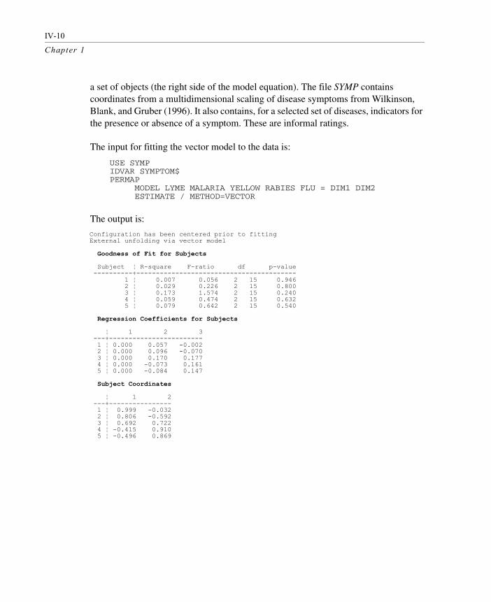
a set of objects (the right side of the model equation). The file SYMP contains coordinates from a multidimensional scaling of disease symptoms from Wilkinson, Blank, and Gruber (1996). It also contains, for a selected set of diseases, indicators for the presence or absence of a symptom. These are informal ratings.
The input for fitting the vector model to the data is:
The output is:
USE SYMPIDVAR SYMPTOM$PERMAP MODEL LYME MALARIA YELLOW RABIES FLU = DIM1 DIM2 ESTIMATE / METHOD=VECTOR
Configuration has been centered prior to fittingExternal unfolding via vector model
Goodness of Fit for Subjects
Subject ¦ R-square F-ratio df p-value ----------+----------------------------------------- 1 ¦ 0.007 0.056 2 15 0.946 2 ¦ 0.029 0.226 2 15 0.800 3 ¦ 0.173 1.574 2 15 0.240 4 ¦ 0.059 0.474 2 15 0.632 5 ¦ 0.079 0.642 2 15 0.540
Regression Coefficients for Subjects
¦ 1 2 3 ---+------------------------ 1 ¦ 0.000 0.057 -0.002 2 ¦ 0.000 0.096 -0.070 3 ¦ 0.000 0.170 0.177 4 ¦ 0.000 -0.073 0.161 5 ¦ 0.000 -0.084 0.147
Subject Coordinates
¦ 1 2 ---+---------------- 1 ¦ 0.999 -0.032 2 ¦ 0.806 -0.592 3 ¦ 0.692 0.722 4 ¦ -0.415 0.910 5 ¦ -0.496 0.869
IV-11
Perceptual Mapping
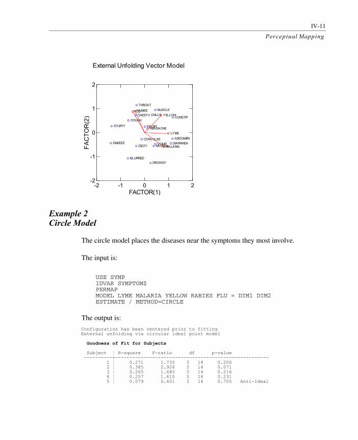
Example 2 Circle Model
The circle model places the diseases near the symptoms they most involve.
The input is:
The output is:
USE SYMPIDVAR SYMPTOM$PERMAPMODEL LYME MALARIA YELLOW RABIES FLU = DIM1 DIM2ESTIMATE / METHOD=CIRCLE
Configuration has been centered prior to fittingExternal unfolding via circular ideal point model
Goodness of Fit for Subjects
Subject ¦ R-square F-ratio df p-value ----------+------------------------------------------------------ 1 ¦ 0.271 1.735 3 14 0.206 2 ¦ 0.385 2.926 3 14 0.071 3 ¦ 0.265 1.685 3 14 0.216 4 ¦ 0.257 1.615 3 14 0.231 5 ¦ 0.079 0.401 3 14 0.755 Anti-Ideal
External Unfolding Vector Model
-2 -1 0 1 2FACTOR(1)
-2
-1
0
1
2FA
CTO
R(2
)
FEVER
DIARRHEA
CONSTIP
NAUSEA
STUFFY
CHEST
HEADACHE
BLURRED
THROAT
ABDOMEN
CHILLSMUSCLE
DROWSY
VOMITCONVULSE
COUGH
DIZZYSNEEZE
LYME
MALARIA
YELLOWRABIESFLU
IV-12
Chapter 1
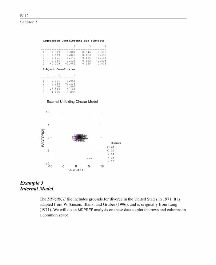
Example 3 Internal Model
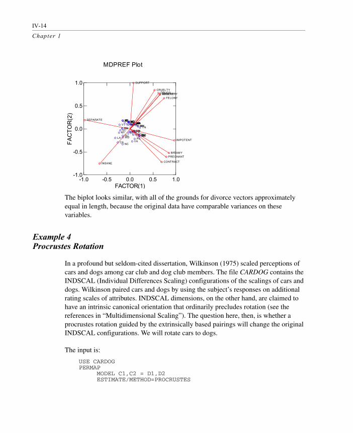
The DIVORCE file includes grounds for divorce in the United States in 1971. It is adapted from Wilkinson, Blank, and Gruber (1996), and is originally from Long (1971). We will do an MDPREF analysis on these data to plot the rows and columns in a common space.
Regression Coefficients for Subjects
¦ 1 2 3 4 ---+---------------------------------- 1 ¦ 0.379 0.001 -0.046 -0.380 2 ¦ 0.449 0.029 -0.123 -0.450 3 ¦ 0.191 0.142 0.155 -0.191 4 ¦ 0.334 -0.123 0.122 -0.335 5 ¦ -0.009 -0.083 0.148 0.009
Subject Coordinates
¦ 1 2 ---+---------------- 1 ¦ 0.001 -0.061 2 ¦ 0.033 -0.136 3 ¦ 0.370 0.405 4 ¦ -0.183 0.182 5 ¦ 4.475 -8.030
External Unfolding Circular Model
-10 -5 0 5 10FACTOR(1)
-10
-5
0
5
10
FAC
TOR
(2)
FEVERDIARRHEACONSTIP
NAUSEASTUFFY
CHESTHEADACHE
BLURRED
THROAT
ABDOMENCHILLSMUSCLE
DROWSYVOMITCONVULSE
COUGHDIZZYSNEEZE
0.00.10.20.30.4R-square
LYMEMALARIAYELLOWRABIES
FLU

IV-13
Perceptual Mapping
The input is:
The output is:
USE DIVORCEIDVAR STATE$PERMAP MODEL ADULTERY..SEPARATE ESTIMATE / METHOD=MDPREF
Configuration has been centered prior to fitting
MDPREF (Biplot) Analysis
Eigenvalues
1 2 3 4 5 6 ------------------------------------------------ 19.196 18.277 9.792 9.132 8.035 6.483
7 8 9 10 11 12 ---------------------------------------------- 4.825 3.595 2.278 0.866 0.581 0.000
Vector Coordinates
¦ 1 2 ----+---------------- 1 ¦ 0.657 0.754 2 ¦ 0.540 0.842 3 ¦ 0.661 0.751 4 ¦ 0.078 0.997 5 ¦ 0.746 0.666 6 ¦ 0.969 -0.248 7 ¦ 0.793 -0.610 8 ¦ 0.626 0.780 9 ¦ 0.694 -0.720 10 ¦ -0.657 -0.754 11 ¦ 0.851 -0.525 12 ¦ -0.982 0.191
Object Coordinates
¦ 1 2 ----+---------------- 1 ¦ 0.102 0.117 2 ¦ 0.048 0.092 3 ¦ -0.032 0.088 4 ¦ -0.152 0.178 . ¦ . . . ¦ . . 49 ¦ -0.165 0.007 50 ¦ 0.176 0.057
IV-14
Chapter 1
The biplot looks similar, with all of the grounds for divorce vectors approximately equal in length, because the original data have comparable variances on these variables.
Example 4 Procrustes Rotation
In a profound but seldom-cited dissertation, Wilkinson (1975) scaled perceptions of cars and dogs among car club and dog club members. The file CARDOG contains the INDSCAL (Individual Differences Scaling) configurations of the scalings of cars and dogs. Wilkinson paired cars and dogs by using the subject’s responses on additional rating scales of attributes. INDSCAL dimensions, on the other hand, are claimed to have an intrinsic canonical orientation that ordinarily precludes rotation (see the references in “Multidimensional Scaling”). The question here, then, is whether a procrustes rotation guided by the extrinsically based pairings will change the original INDSCAL configurations. We will rotate cars to dogs.
The input is:
USE CARDOGPERMAP MODEL C1,C2 = D1,D2 ESTIMATE/METHOD=PROCRUSTES
MDPREF Plot
-1.0 -0.5 0.0 0.5 1.0FACTOR(1)
-1.0
-0.5
0.0
0.5
1.0
FAC
TOR
(2)
AKALARAZ
CA
CO
CT
DE
FLGA
HI
IA
ID
IL
IN
KSKY
LA
MA
MD
ME MI
MNMOMS
MT NB
NC
ND NH
NJ
NMNV
NYOHOK
OR
PA
RI
SC
SD
TNTX
UT
VA
VT WAWI
WVWY
ADULTERYCRUELTY
DESERT
SUPPORT
FELONY
IMPOTENT
PREGNANT
DRUGS
CONTRACTINSANE
BIGAMY
SEPARATE
IV-15
Perceptual Mapping
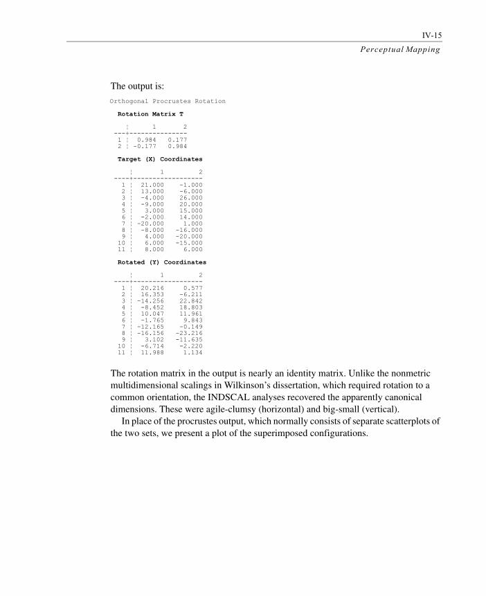
The output is:
The rotation matrix in the output is nearly an identity matrix. Unlike the nonmetric multidimensional scalings in Wilkinson’s dissertation, which required rotation to a common orientation, the INDSCAL analyses recovered the apparently canonical dimensions. These were agile-clumsy (horizontal) and big-small (vertical).
In place of the procrustes output, which normally consists of separate scatterplots of the two sets, we present a plot of the superimposed configurations.
Orthogonal Procrustes Rotation
Rotation Matrix T
¦ 1 2 ---+--------------- 1 ¦ 0.984 0.177 2 ¦ -0.177 0.984
Target (X) Coordinates
¦ 1 2 ----+------------------ 1 ¦ 21.000 -1.000 2 ¦ 13.000 -6.000 3 ¦ -4.000 26.000 4 ¦ -9.000 20.000 5 ¦ 3.000 15.000 6 ¦ -2.000 14.000 7 ¦ -20.000 1.000 8 ¦ -8.000 -16.000 9 ¦ 4.000 -20.000 10 ¦ 6.000 -15.000 11 ¦ 8.000 6.000
Rotated (Y) Coordinates
¦ 1 2 ----+------------------ 1 ¦ 20.216 0.577 2 ¦ 16.353 -6.211 3 ¦ -14.256 22.842 4 ¦ -8.452 18.803 5 ¦ 10.047 11.961 6 ¦ -1.765 9.843 7 ¦ -12.165 -0.149 8 ¦ -16.156 -23.216 9 ¦ 3.102 -11.635 10 ¦ -6.714 -2.220 11 ¦ 11.988 1.134

IV-16
Chapter 1
Computation
Algorithms
The algorithms are documented in the Statistical Background section above. Most involve a singular value decomposition computed in the standard manner.
Missing data
Cases and variables with missing data are omitted from the calculations.
References
Bennet, J. F. and Hays, W. L. (1960). Multidimensional unfolding: Determining the dimensionality of ranked preference data. Psychometrika, 25, 27–43.
Borg, I. and Groenen, P. J. F. (1997). Modern multidimensional scaling: Theory and applications. New York: Springer Verlag.

IV-17
Perceptual Mapping
Carroll, J. D. (1972). Individual differences and multidimensional scaling. In R. N. Shepard, A. K. Romney, S. B. Nerlove (eds.), Multidimensional scaling: Theory and applications in the behavioral sciences, Vol. 1, 105–155. New York: Seminar Press.
Cliff, N. (1973). Scaling. Annual Review of Psychology, 24, 473–506.Coombs, C. H. (1950). Psychological scaling without a unit of measurement.
Psychological Review, 57, 145–158.Dow, B. M. (1990). Nested maps in macaque monkey visual cortex. In K. N. Leibovic
(ed.), Science of vision, 84–124. New York: Springer Verlag. Gabriel, K. R. (1971). The biplot graphic display of matrices with application to principal
component analysis. Biometrika, 58, 453–467.Green, P. E. and Tull, D. S. (1975). Research for marketing decisions, 3rd ed. Englewood
Cliffs, N. J.: Prentice Hall.Kosslyn, S. M. (1981). Image and mind. Cambridge: Harvard University Press.Lilien, G. L., Kotler, P., and Moorthy, K. S. (1992). Marketing models. Englewood Cliffs,
N.J.: Prentice Hall.Long, L. H. (ed.) (1971). The world almanac. New York: Doubleday.Milgram, S. and Jodelet, D. (1976). Psychological maps of Paris. In H. M. Proshansky, W.
H. Itelson, and L. G. Revlin (eds.), Environmental Psychology. New York: Holt, Rinehart, and Winston.
Osgood, C. E., Suci, G. J., and Tannenbaum, P. H. (1957). The measurement of meaning. Urbana, Ill.: University of Illinois Press.
Schönemann, P. H. (1966). A generalized solution of the orthogonal Procrustes problem. Psychometrika, 31, 1–10.
* Schwartz, E. J. (1981). Computational anatomy and functional architecture of striate cortex: A spatial mapping approach to perceptual coding. Visual Research, 20, 645–669.
Shepard, R. N. and Cooper, L. A. (1982). Mental images and their transformations. MA: MIT Press, Cambridge.Wilkinson, L. (1975). The effect of involvement on similarity and preference structures.
Unpublished Ph.D. dissertation, Yale University.Wilkinson, L., Blank, G., and Gruber, C. (1996). Desktop data analysis with SYSTAT.
Upper Saddle River, N.J.: Prentice-Hall.Wish, M., Deutsch, M., and Biener, L. (1972). Differences in perceived similarity of
nations. In R. N. Shepard, A. K. Romney, S. B. Nerlove (eds.), Multidimensional scaling: Theory and applications in the behavioral sciences, Vol. 2, 289–313. New York: Seminar Press.
(* indicates additional reference.)


