
i
STATISTICAL ANALYSIS OF SOCIO-ECONOMIC
DETERMINANTS ON CHILD LABOUR AND SCHOOLING IN
GHANA.
BY
TWUM ERIC OHENEBA
(10084920)
THIS THESIS IS SUBMITTED TO THE UNIVERSITY OF GHANA, LEGON IN
PARTIAL FULFILMENT OF THE REQUIREMENT FOR THE AWARD OF MPHIL
STATISTICS DEGREE.
JUNE, 2015
University of Ghana http://ugspace.ug.edu.gh

ii
DECLARATION
Candidate’s Declaration
This is to certify that this thesis is the result of my own work and that no part of it has been
presented for another degree in this University or elsewhere.
SIGNATURE………………………….. DATE……………………………
TWUM ERIC OHENEBA
(10084920)
Supervisors’ Declaration
We hereby certify that this thesis was prepared from the candidate’s own work and supervised in
accordance with guidelines on supervision of thesis laid down by the University of Ghana.
SIGNATURE……………………………. DATE………………………..
DR. SAMUEL IDDI
(Principal Supervisor)
SIGNATURE………………………….. DATE…………………………..
DR. EZEKIEL N.N. NORTEY
(Co – Supervisor)
University of Ghana http://ugspace.ug.edu.gh

iii
ABSTRACT
The objective of this study was to find the socio-economic determinants of child labour and
schooling in Ghana. To this end, the 2003 Ghana Child Labour Survey data was analysed. The
main techniques used were the simple logistic regression and multilevel logistic regression
analysis. Results of the analysis showed that gender of head of household, marital status of
parents, father’s occupation, mother’s occupation, relationship to head of household, place of
residence, literacy of head of household, sex of the child and highest educational level attained
by parents are all significant determinants of child labour and schooling in Ghana. It was also
found out that if a parent is an unpaid apprentice, it raises the probability that, his/her child will
attend school and work. The children who are sons and daughters of the household head are not
as likely to find themselves in school and work as opposed to other relations living in the
household. In spite of the fact that 10-14 years of age is a typical school going age, in the case of
the groups that were studied, it came out that, majority of this age group were found working.
Children who combined school with work mainly come from parents who are single. These
children lived in urban areas where job opportunities are available.
University of Ghana http://ugspace.ug.edu.gh

iv
DEDICATION
This work is dedicated to my lovely mother, my sweet wife and my precious jewels; Kofi and
Maame.
University of Ghana http://ugspace.ug.edu.gh

v
ACKNOWLEDGEMENT
I thank the Almighty God who has given me care, knowledge and the opportunity to pursue
education up to this level.
There are many people without whom this work could not have been possible. I render my
sincere gratitude’s to my supervisors; Dr. Samuel Iddi and Dr. E.N.N. Nortey for their countless
guidance, advice and constructive criticism throughout this work. I would also like to thank all
the lectures of Statistics Department for their pieces of advice and encouragements throughout
my years of study in this University.
I would also thank my mother, my wife and my only brother for their financial support. I again
thank all my friends and loved ones for their patience throughout my studies. I say the good Lord
continue to bless you.
Finally, to my good friend David Coffie Darko of Presec, Legon for his support and
encouragements and all my friends especially 2015 batch of MPhil Statistics students, I pray for
God’s mercies and favour for you all.
University of Ghana http://ugspace.ug.edu.gh

vi
TABLE OF CONTENTS
CONTENT PAGE
DECLARATION…………………………………………………………………. i
ABSTRACT……………………………………………………………………….. ii
DEDICATION…………………………………………………………………..... iv
ACKNOWLEDGEMENTS……………………………………………………… v
TABLE OF CONTENT…………………………………………………………... vi
LIST OF TABLES………………………………………………………………... x
LIST OF FIGURES………………………………………………………………. xii
CHAPTER ONE: INTRODUCTION…………………………………………... 1
1.1 Background ………………………………………………………….. 1
1.2 Child Labour and Schooling Situation in Ghana …………...………… 6
1.3 Statement of the Problem …………………………………..………… 7
1.4 Objective of the Study ……………………………………………….. 11
1.5 Research Question …………………………………………………… 11
1.6 Research Methodology……………………………………………...... 11
1.6.1 Source of Data………………………………………………... 11
1.6.2 Description of the Data………………………….…………… 12
1.7 Significance of the Study……………………………………………... 12
1.8 Method of Analysis…………………………………………………… 12
1.9 Outline of Dissertation……………………………………………....... 13
CHAPTER TWO: LITERATURE REVIEW………………………….………. 14
2.0 Literature Review…………………………………………………...... 14
University of Ghana http://ugspace.ug.edu.gh

vii
CHAPTER THREE: PRELIMINARY ANALYSIS ………………………….. 29
3.0 Introduction …………………………………………………………... 29
3.1 Data and Scope ………………………………………………….…… 29
3.2 Logistic Regression……………………………………………….…... 30
3.3 The Exponential Family of Distributions ………………………......... 31
3.3.1 Properties of Exponential Family of Distributions…………... 32
3.3.2 Maximum Likelihood Estimation of the
Exponential Family ………………………………………....... 34
3.4 The Generalized Linear Models (GLM) ……………………………... 35
3.5 The Basic Logistic Regression Model ……………………………...... 37
3.5.1 Assumptions Underlying Logistic Regression……………….. 38
3.5.2 Application of Logistic Regression …………………………. 39
3.6 The Odds ……………………………………………………………... 39
3.7 The Odds Ratio ………………………………………………………. 40
3.8 Estimation of Model Parameters ……………………………………... 41
3.8.1 Maximum Likelihood Estimator (MLE) …………………….. 41
3.9 Testing the Goodness-of-Fit ………………………………………… 43
3.9.1 Deviance and Likelihood Ratio Tests ……………….………. 43
3.9.2 Pearson’s Chi-square Test …………………………….…....... 45
3.9.2.1 Phi and Cramer V Test ………………….…………. 46
3.9.3 Pseudo R-Square ………………………………………..…… 47
3.10 Test of Individual Model Parameters ……………………...……....... 48
3.10.1 The Likelihood ratio Test …………………………………... 48
University of Ghana http://ugspace.ug.edu.gh
viii
3.10.2 Wald Statistic ………………………………………………. 49
3.11 Confidence Interval Estimation…………………………………....... 49
3.12 Multilevel Modelling Approach to Clustered Data ………………… 50
3.12.1 Cluster-Specific Models……………………….……………. 51
3.12.2 Generalized Linear Mixed Models (GLMM)….…………… 51
CHAPTER FOUR: FURTHER ANALYSIS ………………………………….. 53
4.1 Preliminary Analysis …………………………………………………. 53
4.1.0 Introduction ………………………………………………….. 53
4.1.1 Characteristic of Sample …………………………………….. 53
4.1.2 Occupation of Children’s Parents …………………………… 63
4.1.3 Education of Parents ………………………………………… 64
4.1.4 Marital Status of Parents …………………………………….. 65
4.1.5 Regional Distribution of Children …………………………... 65
4.1.6 Ethnicity……………………………………………………… 67
4.1.7 Measurement of Children’s Work …………………………... 71
4.1.8 Activity Status of Children ………………………………….. 73
4.2 Further Analysis ……………………………………………………... 75
4.2.0 Introduction ………………………………………………….. 75
4.2.1 Findings ……………………………………………………... 76
4.2.2 Model for Children’s Schooling and Working
Using Logistic Regression ………………………………........ 76
4.2.3 Characteristics of Children…………………………………... 80
4.2.4 Characteristics of Parents ………………………………......... 81
University of Ghana http://ugspace.ug.edu.gh

ix
4.2.5 Characteristics of Household ………………………………... 82
4.2.6 Multilevel Analysis ………………………………………….. 83
CHAPTER FIVE: SUMMARY, DISCUSSIONS, CONCLUSIONS
AND RECOMMENDATIONS ……………………………… 89
5.1 Summary……………………………………………………………. 89
5.1.1 Limitations of the Study………………………………............ 91
5.1.2 Study Strengths ……………………………………………… 92
5.2 Discussions ………………………………………………....……….. 92
5.3 Conclusions ………………………………………………………… 94
5.4 Recommendations …………………………………………………. 95
REFERENCES………………………………………………………………...…. 97
APPENDICES……………………………………………………………..……… 106
University of Ghana http://ugspace.ug.edu.gh

x
LIST OF TABLES
Table Page
Table 4.1: Distribution of Children Aged 5-17 Years by Region …………………... 54
Table 4.2: Sex Distribution of Children Combining Schooling
and Economic Activity by Age and Locality of Residence ……………... 55
Table 4.3: Average Age of Children by Region…………………………………….. 56
Table 4.4: Average Household Size by Region…………………………………....... 57
Table 4.5: Average Enrollment Age by Level of Schooling and
Grade Completed……………………………………………………....... 58
Table 4.6: Percentage Distribution of Non-Working and Working
Children by School Attendance………………………………………….. 58
Table 4.7: Percentage Distribution of Non-Working Children by Sex……………… 59
Table 4.8: Percentage Distribution of Non-Working and Working
Children by Relationship to Head of Household………………………… 60
Table 4.9: Percentage Distribution of Non-Working and Working
Children by Age Group………………………………………………….. 60
Table 4.10: Percentage Distribution of Non-Working and Working
Children by Size of Household…………………………………………... 61
Table 4.11: Percentage Distribution of Non-Working Children by
Age of Household Head…………………………………………………. 62
Table 4.12: Percentage Distribution of Working and Non-Working
Children by Literacy of Household Head……………………………….. 63
University of Ghana http://ugspace.ug.edu.gh

xi
Table 4.13: Percentage Distribution of Working and Non-Working
Children by Major Occupation of Parent……………………………….. 63
Table 4.14: Percentage Distribution of Working and Non-Working
Children by Level of Education of Parent………………………………. 64
Table 4.15: Percentage Distribution of Working and Non-Working
Children by Parent Marital Status………………………………………. 65
Table 4.16: Percentage Distribution of Working and Non-Working
Children by Region…………………………………………………....... 66
Table 4.17: Percentage Distribution of Working and Non-Working
Children by Ethnicity…………………………………………………… 67
Table 4.18: Percentage Distribution of Working and Non-Working
Children by Locality of Residence……………………………………… 68
Table 4.19: Percentage Distribution of Working and Non-Working
Children by Sex of Head of Household…………………………………. 68
Table 4.20: Reason for Leaving School…………………………………………....... 71
Table 4.21: Activity Status of Children by Sex and Age…………………..………... 73
Table 4.22: Omnibus Test of Model Coefficients…………………………………… 77
Table 4.23: Model Summary………………………………………………………… 77
Table 4.24: Classification Table for Binary Logistic Regression……………………. 78
Table 4.25: Model 1: Parameter Estimate for Schooling Status of
Children Using Binary Logistic Regression…………………………….. 79
Table 4.26: Classification Table for the Intercept only Model………………………. 84
Table 4.27: Classification Table for the Null Model………………………………… 84
University of Ghana http://ugspace.ug.edu.gh

xii
Table 4.28: Model 2: Parameter Estimates for Schooling Status
Of Children Using Multivariate Logistic Regression…………………… 86
Table 4.29: Covariance Parameters for the Null Model……………………………... 88
Table 4.30: Covariance Parameters for the Full Model (Model 2)…………….......... 88
University of Ghana http://ugspace.ug.edu.gh

xiii
LIST OF FIGURES
Figure Page
Figure1: Children Not Enrolled in School by Age…………………………........ 67
Figure 2: Children Not Enrolled in School by Age and Sex……………………. 70
Figure 3: Distribution of Children by Activity Status………………………....... 72
University of Ghana http://ugspace.ug.edu.gh

1
CHAPTER ONE
1.0 INTRODUCTION
1.1 Background
Children„s development has become a very important issue to all countries in the world. It is
realized that the future of any country depends on how the country takes care of her children.
Child labour levels are high in many developing countries. Any activity, economic or non-
economic, performed by a child, that has the potential to negatively affect his/her health,
schooling and normal developments constitute child labour.
According to recent International Labour Organization‟s (ILO) estimates, about 211 million
children aged 5-17 years were economically active globally (ILO-IPEC, 2002). About 73
million of these working children were below 10 years. The highest number of child workers in
the age group 5-17 years is found in Asia-Pacific (127.3 million) followed by sub-Saharan Africa
(48 million), Latin America and the Caribbean (17.4 million) and Middle East and North Africa
(13.4 million). While Asia has the highest number of child workers, sub-Saharan Africa has the
highest proportion of working children. In Ghana some children stop school or do not attend
school in order to work.
In the Ghanaian context, the incidence of child labour is considered very high. According to the
2003 Child Labour Survey of Ghana, 38.9 percent of the 6,361,178 children in the age group
5-17 years were, found to be economically active (GSS, 2003). This puts the child labour force at
about 12 percent of the total labour force of Ghana.
University of Ghana http://ugspace.ug.edu.gh

2
The highest proportion of child labourers in Ghana is found in agriculture/fishing/forestry
(57.0%), followed by sales (20.7%), production (9.5%). The rest were engaged throughout the
text as truck-pushers, porters, labourers, driver-mates (11.0%). The major occupation for both
males (69.0) and females (44.0) is Agriculture, Fishing and Forestry. Another major occupation,
for females, is sales (30.4%) (GCLS, 2003).
Although in Ghana, child labour attracts most international attention, child labour is much more
common in the rural informal sector. Statistics on child labour in Ghana and other developing
countries also reveal that a vast majority of working children are employed in domestic service
where children perform household chores such as fetching water, collecting firewood, cooking
and taking care of younger siblings. Although many of these children are working under family
supervision, full-time work can deter them from attending school, and many home-based
activities can be as harmful as work performed outside the home.
In our Ghanaian society, it is a tradition that children engage in all kinds of work, which forms
part of their training. Unfortunately, the rate at which these children flock the streets of Ghana
for economic ventures these days in a bid to assist parents has assumed increasing dimensions
and therefore questionable. It is these observations that have aroused the interest to research into
these areas to look into the reasons why children engage themselves actively in economic
activity while schooling and the effects this practice has on their development.
According to Safo (1990), Ghana was the first country to ratify the convention on the rights of
the child, “Ghana demonstrated to the world her preparedness to promote the cause of children to
new and higher levels and to abide by the provisions of the convention”. The year 1990
University of Ghana http://ugspace.ug.edu.gh
3
witnessed the arduous drafting process within the U.N. Commission on human rights, which
culminated in the 54th article convention outlining the rights of children. The law was in favour
of states which could not meet the rights of their children due to lack of resources. The law made
available three areas of assistance to states in need: provision, protection and participation.
Firstly, children were provided with the right to life, to name and to freedom of taught, conscious
and religion. Secondly, they were protected from physical and mental violence with special
attention paid to the protection of children who were disabled or belonged to minorities or who
were refugees. Lastly, the convention also provides for the child the right to be heard on
decisions affecting his or her life. Its continuation, however, was a step towards the provision of
minimum standard of treatment.
In a similar vein, the Education Acts 1961 (Act 87) provides for compulsory education for every
child in Ghana who had attained the school going age. Another declaration of the rights of the
child is the U.N. Declaration of the Rights of Children, Article 9 which states in part that “The
child shall be protected against all forms of neglect cruelty and exploitation. He shall not be the
subject of traffic in any form”.
According to the labour amendment Decree 1973 (NRCD 150) section 44 of NCD 157 of Ghana
among other things provided that “No person shall employ a child except where the employer is
with the child‟s own family and involves in a light work of agricultural or domestic character
only”. Sanction for non-observation of this provision is the imposition of a fine or summary
convention of the culprit. Section 47 of this law defines a child as a person under 15 years old.
This particular law is debatable with the reason that farm work for one is known to be very
University of Ghana http://ugspace.ug.edu.gh

4
tedious and cannot be termed high work besides; it is this work that almost children in the rural
areas are introduced to.
In a keynote address delivered by Attorney General and Provisional National Defence Council
Secretary for Justice at a National Workshop on Child Labour (10th-14th August,1988), noted that
legislation was not enough to curb child labour. He pointed out that children are prevented from
going to school because of the activities they find themselves in. These activities include fishing
and hawking. It was unlawful to prevent a child from going to school. However, the Education
Act 1961(Act 87), provides for compulsory education of every child in Ghana who has attained
the school-going age. Under section 2(2), any parent who fails to comply with provisions of the
preceding subsection commits an offence and shall be liable on summary conviction to a fine.
But a legislation that is not enforceable is meaningless. The fact is that the government cannot
afford a fee-free education policy any more, what then is the justification for prosecuting a parent
for non-conformity to the Education Act? For most parents, a child must first of all eat before he
or she can go to school. Besides, sending a child to school does not mean paying the school fees,
which is only manifest function, but also supplying latent demands like school uniforms and in
certain instances provide table and chairs and stationery. One setback of the Education Act,
therefore is that, it assumes that educational facilities are easily available and affordable. In
1988, out of 2.2 million pupils of school-going age, only 1.3 million were in school. Here the
intake facilities were not just there. The Attorney- General also quoted the Labour Decree 1976
(NLCD 157) section 44 (1), which states that: “No person shall employ a child except where the
employment is with the child‟s own family and involves light work of an agricultural or
University of Ghana http://ugspace.ug.edu.gh

5
domestic character only”. It is however, not clear in his decree the limits and boundaries of what
qualifies to be light work of an agricultural or domestic character.
Another important law which protects the interest of the child is section 79 of Criminal Code
(Act 29) states that: “A man is under duty to supply the necessaries of health and life to his wife
being actually under his control and to his legitimate and illegitimate son or daughter, being
actually under his control and not being of such age and capacity as to be able to obtain such
necessaries. A guardian is under the like duty with respect to his ward being actually under his
control”. Also, the law has not been able by its mere existence to ensure the provision of
“essential necessaries” of health and life to children in Ghana.
A representative of the National Council on Women and Development‟s (NCWD), drew
attention to female domestic servants, some of whom find themselves in this role because the
traditional notions about females was that, formal education is not important to them. This was
because they ended always in the kitchen. She also made reference to children who got married
at very tender ages as low as twelve years old. At this tender age they become vulnerable to
exploitation by members of their husband‟s family.
The NCWD is sympathetic towards children in work roles. They did not advocate for its total
abolition but rather were interested in securing a minimum age for child work and the provision
of adequate remuneration for it. Apart from their concern on a minimum age of employment,
they also suggested that the law on compulsory education must be enforced. Parent must be
penalized for trading their children off instead of sending them to school. Whether this
enforcement is possible is another question.
University of Ghana http://ugspace.ug.edu.gh

6
The views of the Ghana Education Service were on opinion that, child labour has been generally
accepted as a means of solving chores. It is the result of polygamy and it adds cumulatively to
the illiteracy rate.
According to Dr. Abdullah (1978) (then Secretary for Education in Bangladesh), “the most
disturbing aspect of this problem of school is that 40 percent of the children of school-going age
are not in school. Moreover, enrolment ratio in the southern half of the country is double those of
the northern half”. The problems were not only a question of enrolment, but also a problem of
drop out or sustenance of those who are already in school. In 1984, the drop-out rate was 36.58
percent. In addition, the quality of teachers was also a problem. Dr. Abdullah, (1985) said
“untrained teachers of the primary school form 48 percent while at the Middle School; they
formed 38 percent of all the teaching staff”. It is difficult to see how the interest of the children
could be sustained at school given these relatively low skilled personnel.
On the contrary, the Ghana Education Service had not only recognized that child labour was a
problem but had also made attempts as to how they could attack this problem. This review
therefore offers an opportunity for all especially policy planners and parents to take a new look at
children engagement in economic activities and educational aspirations.
1.2 Child Labour and Schooling Situation in Ghana
The official age of entry into primary school is 6 years (according to the Primary Education Act,
1992), although many children attend primary school at the age of 4 or 5 years. Late entry into
primary school is also very common in rural areas.
University of Ghana http://ugspace.ug.edu.gh

7
In Ghana, primary education is compulsory for all children. The Government has introduced the
Free Compulsory Universal Basic Education (FCUBE) to get all children of school going age to
school and to prevent children from early labour. According to the Ghana Primary School Act
(1992), a child of 6 years old must go to school. To make the school attendance easier especially
for children from poor parents, textbooks are supplied free of charge to all children up to Junior
Secondary School (JSS). An alternative subsidy program (the School Feeding Programme) or
(Food-For Education), has been implemented to help children and their parents. In-spite of all of
these measures, a large proportion of children are not enrolled in school.
This study therefore examines the socio-economic factors which account for school children‟s
engagement in economic activities in Ghana.
1.3 Statement of the Problem
The high incidence of child labour in many developing countries, including Ghana, may be
attributed to socio-cultural norms in these settings. In the olden days children were considered as
factor of production; labour force for the family. This was not a problem because, in the absence
of modern technology majority of the parents had to depend on their children as sources of
labour especially in the cocoa growing areas, fishing communities and others where manual
labour was most certainly required.
Traditionally, children predominantly feature in the family upkeep in many ways. However, it is
this mode of contribution today due to social change and money-using economics that raises an
enquiry and understanding of the phenomenon.
University of Ghana http://ugspace.ug.edu.gh

8
Most often the labour force of a nation consists of men, women and children. The employment of
children is socially and legally determined as illegal because in most countries, children with
minimum age (usually 15 years) are not legal to be used for full time employment. However, it is
their mode of contribution where they are employed mostly in commercial activities that have
been the major concern for the working child, families and the society as a whole. This high
incidence of child labour and the subsequent low school attendance rates in Africa has attracted
the attention of most governments, past and present. This is evidenced by a constant search for
adequate measures to arrest the situation. The issue of child labour is a major concern of the
Government of Ghana, as it is for many other countries. The problem has long been recognized
and the Government has enacted laws to prohibit child labour, increase school enrolment rates
and develop other national programmes to meet the urgent needs of children in the country.
In spite of these efforts, millions of children continue to work as forced labourers in a wide range
of sectors, industries or occupations either to pay for the debts of their parents or to help earn
income for their care givers. In some instances, these children are drawn into certain economic
activities under false pretexts from which they are not allowed to leave.
Many countries have undertaken labour force surveys that define participation in the labour force
as being engaged in „economic activity‟. Such surveys do not adequately capture participation in
economic, but illegal activity, work that is unpaid for and undertaken in household enterprises
whose product is mainly for household consumption. Also, some activities, while certainly
involving work, were not deemed „economic‟ and are therefore excluded from such surveys.
While many of these problems arise in canvassing information about adults as well as children,
they are particularly severe in canvassing information about the work of children.
University of Ghana http://ugspace.ug.edu.gh

9
Another serious problem involves children who are neither classified as economically active nor
as students enrolled in or attending schools. In parts of Africa where child fostering is prevalent,
it is often difficult to determine whether this is in fact disguised child labour. As such, economic
activity as a proxy for child labour could understate the number of working children.
Children perform different types of work under a variety of conditions and for a variety of
reasons. Therefore, in assessing child labour, the types and conditions of work, the age of the
children who perform the work, and the developmental level of the country must all be taken into
account. This is because not all child work is considered to be detrimental to the growth and
well-being of children.
The ILO defines light work as work that is not likely to be harmful to children‟s health or
development and not likely to be detrimental to their attendance at school or vocational training.
In determining whether work is likely to be harmful, the ILO takes into consideration the
duration of work, the condition under which the work is done, and the effect on school
attendance, among other factors. However, the ILO does not provide any operational guidance
for assessing these factors and determining whether any given form would qualify as light work.
Hazardous work includes „work which by its very nature or the circumstances in which it is
carried out is likely to jeopardize the health, safety or moral of young persons‟ (International
Labour Organization, 1973). It is left to individual governments to determine which types of
work fall under the rubric of light or hazardous.
University of Ghana http://ugspace.ug.edu.gh

10
Most children in Ghana are not able to pursue their education these days as is expected of them.
This problem is attributed to the fact that children are often actively engaged in economic
activities while attending school, they are seen hawking, cracking stone, farming, weaving kente
cloth for money. As a result, most of them are not able to complete their elementary education.
Besides, what they hope to become in future is either hindered or not achieved. Another
unfortunate aspect of the whole issue is that, these children tend to pick up some kind of
behavior like disrespect and the practice of deliberately staying away from school without
permission. Furthermore, some of these children later „drop-out‟ of school because they are
either not able to perform well in class or have more interest in working for money than
schooling.
Schooling and other forms of education can help to lower the incidence of child labour. However
the pace of reducing child labour and improvement in school participation rates is somewhat
slow in Ghana. In a number of developing countries, targeted enrollment subsidies have been
used as an effective way to break the cycle of poverty and illiteracy and address both the income
loss to parents and education for children. This problem is all over the country and need to be
redressed. In order to implement effective child labour policies and schooling programmes, there
is the need to isolate the factors that contribute to child labour which in turn affect school
enrolment rates. In 2001, the Ghana Statistical Service organized a child labour survey, within
the framework of the IPEC, to facilitate the assessment of the impact of policies and programmes
that had been implemented in Ghana to reduce child labour. This study therefore examines the
socio-economic factors which account for school children‟s engagement in economic activities
in Ghana.
University of Ghana http://ugspace.ug.edu.gh

11
1.4 Objectives of the study
The general objective of this study is to determine the socio-economic factors that influence
child labour and schooling in Ghana.
The specific objectives are:
(i) To determine socio-economic factors contributing to child labour and schooling.
(ii) To determine socio-economic factors causing school children‟s engagement in
economic activity.
(iii) To establish the relationship between child labour and schooling,
(iv) To make recommendations, based on the findings, for appropriate intervention
measures to reduce child labour.
1.5 Research Questions
In line with the above objectives, the study poses the following research questions:
(i) What are the major socio-economic factors that contribute child labour and schooling?
(ii) What are the socio-economic factors causing school children‟s engagement in economic
activity?
(iii)What is the relationship between child labour and schooling?
1.6 Research Methodology
1.6.1 Source of Data
The main source of data for this study was the Ghana Child Labour Survey (GCLS,2003), the
Ghana Living Standard Survey Round Six (GLSS6) : Labour Force Module, administered by
Ghana Statistical Service (GSS, 2013), and other secondary sources were also utilized.
University of Ghana http://ugspace.ug.edu.gh
12
1.6.2 Description of the Data
The sample design and sampling procedure for used for the Ghana Child Labour Survey (GCLS)
comprised both a nationwide probability sample survey of all households in Ghana and
supplementary non-probability survey of street children.
The questionnaire collected information on housing/household characteristics, socio-
demographic characteristics of all household members, information on economic activity, and
other conditions of children.
1.7 Significance of the Study
(i) The study is geared towards providing the necessary statistical justification regarding
socio-economic determinants of child labour.
(ii) The study will furnish decision makers and other stakeholders with information regarding
the major socio-economic determinants of child labour and schooling in Ghana.
1.8 Method of Analysis
In this study, bivariate distributions of child labour are carried out to examine the relationship
between child labour and their covariates. In order to make full use of available information,
these bivariate investigations were limited to children aged 5-17 years that are working and not
working.
The study also examined the data structure to find out if multilevel models can be applied to
these data to determine the extent of familial and clustering effects. Multivariate analyses are
then conducted to identify the factors which have influenced recent child labour levels. The
University of Ghana http://ugspace.ug.edu.gh

13
multivariate analytical models applied are standard logistic regression models and multilevel
logistic regression models. The results of this research are compared to those obtained by others
to identify the factors which contributed to child labour and schooling in Ghana.
1.9 Outline of Dissertation
The study comprises five chapters. Chapter one presents the background of the study, problem
statement, objective, research questions, methodology, significance and outline study. Chapter
two reviews some of the relevant literature related to the work. This is followed by chapter three,
which presents an in-depth discussion of the methodology employed. Chapter four presents
detailed analysis and discussion of results. Summary, conclusions and recommendations are
captured in the fifth chapter.
University of Ghana http://ugspace.ug.edu.gh

14
CHAPTER TWO
LITERATURE REVIEW
Significant differences in child labour and schooling exist among populations in nearly all
countries. Studies have identified specific significant determinants to include educational
attainment, occupational status, marital status and place of residence.
Zelizer in 1994 addressing a conference on child labor in America, stated that, “The term „„child
labour‟‟ is a paradox, for when labour begin… the child ceases to be” (Wise, 1910). The
International Labour Organization‟s (ILO) new convention on child labour was both an advance
and a strategic retreat from the minimum age standards set by its 1973 Convention No. 138
which states that, all children under 18 years of age, should not be engaged in economic
activities (ILO, 1999). But Convention No. 182 also signals a retreat from the ILO‟s offensive
against child labor (Comparative Education Review). Comparativists should observe that, in
Conversion No. 182, work preventing school access or success is not, in itself, viewed as
inherently intolerable, nor is it to be prioritized for immediate eradication. This geopolitical
novelty can be seen in the context of ongoing debate over the educational implications of the
emerging global market for skills, products, and services.
The ILO‟s new approach highlights the centrality of child welfare for researchers and advocates
of education. A case in point: What do we know about the effects of „„globalization‟‟ for
children‟s work and schooling? In many ways, international markets and the world
institutionalization of children‟s rights through the Convention on the Rights of the Child (CRC)
carry contradictory, even paradoxical implications. On one hand, there are more opportunities for
University of Ghana http://ugspace.ug.edu.gh

15
cash-compensated work; there is also greater inequality, along with new „„needs‟‟ of children for
products advertised by global markets. On the other hand, there is a growing sense that children
should be students, not workers (Nieuwenhuys, 1996). Out of this contradiction, and from
distinct professional orientations, a rich but still very disparate literature is emerging (including
children‟s literature).
Rosenberg (1993) provided a critical counterpoint to advocate for street children who exaggerate
the numbers in order to draw attention to the neoliberal orientations they believe have worsened
their plight. In the first chapter of her book, gave an invaluable history of the discourse over
street children, tracing the worldwide dissemination of this concept to a UNICEF advisor who
suggested in 1981 that there were 100 million street children in the world, half of whom were in
Latin America (Black, 1986). In later estimates, UNICEF continued to revise downward the
number of street children. Meanwhile, by the mid-1980s, Brazilian UNICEF offices estimated
that there were 1.9 million abandoned children and 13.5 million needy children in that country.
But only since the mid-1980s have there been systematic investigations of the status of Brazil‟s
children.
In the early 19"' century, there was an extensive use of child labour over the entire world.
Children often started to work within their family activities (Shah, 1985). This kind of labour has
been seen as part of the integral process of the socialization and training of children for adult
responsibilities (Estrella, 1994). Today, participation of children in the workforce is on the
increase in many parts of the world particularly in the developing countries (Pinto, 1989).
University of Ghana http://ugspace.ug.edu.gh

16
In Ashanti region of Ghana, Rettray (1927) mentioned among other things that, male children
followed their fathers to farm, tended animals like cattle and goats, which form part of their
socialization process. They also learnt crafts like kente weaving and goldsmithing. Oppong
(1973), in his research also observed that, male children follow their fathers or learn to become
butchers, barbers, blacksmiths, farmers and drummers while the girls help in the home routine
tasks like sweeping, cooking and also carry farm produce home, pick legumes and fruits.
Among the Anlos in the Volta region, Nukunya (1969), in his research into child training
mentioned that children enjoy freedom until about 10 years when they are introduced to various
occupations like farming and fishing which is their major work. Boys are taught to pursue
economic activities, which give them substantial income to enable them alleviate their
dependence on their parents. The girls on the other hand, help their mothers in female
occupations like petty trading, baking and fish smoking.
Busia‟s social survey (1950), of Sekondi Takoradi also revealed that boys and girls engage in
several activities that deal with money as a predominant way of life. In the same vein, Acquah in
a survey work in Accra revealed that 30% of the total number of school children in selected
districts in Accra were gainfully employed in activities like selling at the markets, carrying fish
from the beach to the market, domestic servants and newspaper vendors (Acquah, 1972).
Children‟s engagement in work roles in our Ghanaian traditional society is not a new practice.
According to Mends et al. (1988) research work on the native and problems of child labour
stated that children‟s involvement in work roles form part of their training into adulthood.
University of Ghana http://ugspace.ug.edu.gh

17
The rapid growth of the manufacturing sectors (Banerjee. 1995) and poverty (Damodaran, 1997)
may form the common reasons of child labour. On the one hand, the child is a cheap labourer,
obedient and less likely to strike (Trattner, 1970). On the other hand, working children were an
important resource for significant and early contributions to the household income (Cain, 1977).
However, the view those children make a significant contribution to the household income
encourages many families to have more children (Mamdani, 1972).
Accurate statistics on the prevalence of child labour are not available. According to estimates of
ILO, 100-200 million children less than 15 years were working (Habenich, 1994), (Pollack et al.,
1990). This is thought to be an under-estimated value (Ashagrie, 1997) since in some countries,
many young workers below the age of 15 are not included in the labour force statistics because
of the large variety of terms used to describe the notion of childhood and labour (Shah, 1985).
Children who both work and attend school are usually considered as pupils rather than workers.
Moreover, in most countries child labour is clandestine and hidden (Habenich, 1994).
According to Rosemberg (1999), all researchers soon agreed that small numbers of children and
adolescents in metropolitan areas lived apart from either parents. Given that any number of
children living on the street is unacceptable and that little is to be gained by erroneous
estimations, Rosemberg argues that some of the previous characterizations of street children by
UNICEF are at best inflated and at worst self-serving.
Children appear to be involved in a wide range of economic activities. They are engaged in
waged labour in agriculture, services, factories, self-employment in street trades and domestic
services. Some receive part of their wage in kind and many others are unpaid and work for their
University of Ghana http://ugspace.ug.edu.gh
18
families, relatives or friends in the home or on the land. Some others are engaged in marginal
economic activities on the streets and are exposed to drugs, violence, criminal activities and
abuse that damage their health, morals, and emotional development (Heward, 1993).
Large numbers of child labourers start work before 8 years of age. For example, in the carpet
industry, they are preferred to adults because of their docility, fast fingers, low cost and they are
less demanding, (Rodger and Standing, 1981). Under the supervision of ILO, four surveys on
child labour were carried out in urban and rural areas of Ghana, India, Indonesia, and Senegal
during the period of 1992-93. (ILO, 1996). The surveys intended to collect relevant statistics on
the child labour phenomenon. 4000 to 5000 households, both urban and rural, in each of the four
countries were selected as the study sample.
The results of the survey showed that slightly more than 10% of children between the age of 5
and 15 years were found to be economically active during the twelve months prior to the survey.
In Ghana, 80% of working children were engaged in trading activities, about 40% of whom were
working for more than 8 hours per day. More than two thirds were unpaid family workers, while
the average monthly income of 75% of paid workers was far lower than the national minimum
wage.
In the city of Enugu, a study conducted by Asogwa on 400 street hawkers under the age of 15
years and 200 control non-working children with the aim of studying the sociomedical aspects of
child labour in Nigeria, showed that the average age of working children was about 12 years, and
33% of them worked more than 7 hours per day (Asogwa, 1986).
University of Ghana http://ugspace.ug.edu.gh

19
Children work for a variety of reasons. Many authors state that child labour is rooted where
households are suffering of low income, poor living conditions, high unemployment rate and
insufficient opportunities for education (Blanchard, 1983). Poverty emerges as the most
compelling reason why children work. Poor households need money to ensure survival and
children are the only means within their choice and capacity to do that. Children work even
though they are not well paid because they still serve as major contributors to family income in
many parts of the world.
In developing countries, the decision to send children to school or to work is likely to be based
on the relative rate of each return. The costs of education are relatively very high for poor
households sometimes preventing them from sending their children to school and consequently
leading to high rates of child labour (Addison et al., 1997).
Illiterate or low educated parents may not be aware of the importance of educating their children.
Moreover, these parents are more interested to send their children to work rather than to school
because their contribution to household income is highly needed, since the illiterate parents are
usually unskilled people with low income. Thus, with illiteracy among adults, child labour tends
to increase.
Patrinos and Psacharopoulos (1995) used multiple regression to show that factors predicting an
increase in child labour also predict reduced school attendance and an increased chance of grade
repetition. The authors estimated this relationship directly and show that child work is significant
predictor of age-grade distortion (Patrinos and Psacharopoulos, 1997). Akabayashi and
Psacharopoulos (1999) showed that, in addition to school attainment children‟s reading
University of Ghana http://ugspace.ug.edu.gh
20
competence decreases with child labour hours. In addition, Heady (2003) used direct measures of
reading and mathematics ability and finds a negative relationship between child labour and
educational attainment in Ghana.
All of these papers examine the correlation, rather than the causal relationship between child
labour and schooling outcomes. However, Cavalieri (2002) used propensity score matching and
finds a significant, negative effect of child labour on educational performance. Ray and
Lancaster (2003) instrument child labour with household measures of income, assets and
infrastructure, to analyze its effect on several school outcome variables in seven countries. But
their instrumenting framework is questionable, as they make the strong assumption that
household income, assets, and infrastructure are exogenous to the schooling equations.
In order to test whether child labour is efficient or not, Baland and Robinson, (2000) assumed
that there is a trade-off between child labour and the accumulation of human capital.
Child labour is perceived to be a serious problem as it is believed to be destructive to children‟s
intellectual and physical development, especially that of young children. The danger is
exacerbated for those children who work in hazardous industries. This is the theory behind the
„child labour trap‟ – if a child is employed all through the day, the child remains uneducated and
subsequently has low productivity as an adult so child labour can directly contribute to adult
unemployment in developing countries. A major caveat of the literature to date is that there is
very little treatment of such long-term dynamic consequences of child labour.
University of Ghana http://ugspace.ug.edu.gh

21
The accessibility and quality of education and its relevance to the labour market is one factor in
parents‟ decision to send their children to school. Although, as many boys and girls combine
school attendance and work increased enrolment rates can have an effect on working hours and
on the kind of work done (Sudharshan/Coulombe (1997), Odonkor (2007), Ghana Statistical
Service (2003).
However, as Odonkor (2007) claims, “rural parents should rather be seen as dissatisfied clients
of the educational system than as illiterates, ignorant of the value of education”. It is striking that
although about 90 percent of the children in cocoa growing areas are enrolled in schools, 54
percent cannot read or write (MMYE/NPECLC 2008). Because of the poor quality of schools,
the difficulties of access and the uncertainties about finding an adequate job after graduation,
parents have developed a strategy to spread the risks, which involves sending some of their
children to school while others help with fishing, farming or other economic activities.
The findings of this case study are in line with the research done by Kufuogbe (2005) on children
in fishing in the Central Region, both with regard to the kind of work they do and to the
remuneration they receive. Based on a quite large sample of 356 children, from randomly
selected households, several schools and landing sites using multiple regression. He estimates
that 10 to 20 percent of the children living in coastal areas are involved in fishing, especially in
the main season. The author concluded that being at the beach has become a “way of life” for
them, allowing them both to earn an income and to play and swim for leisure, (Kufuogbe, 2005).
University of Ghana http://ugspace.ug.edu.gh

22
The daily routines for cattle boys in North and South Tongu are similar. They also work for ten
to twelve hours a day, mostly from 6-8 am in the morning to 6 pm in the evening, seven days a
week. Their main tasks are to herd cattle to the field at an agreed time to graze and drink, to
ensure that the animals do not destroy people‟s farms and that they do not get lost or stolen. In
addition, the boys help with other husbandry activities such as spraying and bathing the cattle.
Some also have to collect firewood for the cattle owner‟s wife before they can eat and leave for
the field. The boys operate in teams of up to three. Most of them eat twice a day, mainly
breakfast and supper. For lunch, they hunt for rodents and gather fruit or catch fish from nearby
waters, (Afenyadu, 2008).
Nearly every study on the relationship between child labour and education compares the
educational outcomes of children who don‟t work, or who work less, and those who do work, or
work more. The first hurdle that needs to be surmounted, then, is accurate measurement of both
these variables. “Education” is difficult to define and measure because it is multi-faceted. It can
take the form of school attendance, school performance or skill acquisition, and each of these can
be approached in more than one way. But child labour is also far from simple to measure.
Most children who work are engaged in household enterprise activities, whether it is a farm, a
home-based manufacturing operation, or a retail enterprise. The productive assets would have
mixed impacts on child labour. On the one hand, they may raise a child‟s opportunity cost of
time in school because the child is productive in labour activities. On the other hand, adults in
the household are also more productive, so the household can better afford allocating child time
to schooling activities. Cockburn (2000) used the productivity model to explains why some
University of Ghana http://ugspace.ug.edu.gh

23
agricultural households used measures of the farm capital stock to lower child labour, while
others find the opposite (Rosenzweig and Evenson, 1977).
According to Cockburn & Dostie (2007), it is not always the poorest households that engage in
child labour. While household income draws children out of school, the productivity effect of
underlying greater asset holdings does the contrary. Beegle, Dehejia and Gatti (2006) found out
that there is a positive and significant relationship between the level of household assets and the
use of child labour. This is initially surprising (since child labour is normally portrayed as being
negatively associated with household wealth), but in agricultural settings a positive association
can be rationalised. Rural households with larger farms are more likely to demand higher levels
of child labour from their children.
Graitcer and Lerer (1998) provided a comprehensive international review of the state of
knowledge of the impact of child labour on health. Data on the extent of child labour itself is
subject to considerable error, but data on the incidence of child injuries on the job are even more
problematic. Sources of information come from government surveillance, sometimes
supplemented by data from worker‟s compensation or occupational health and safety incidence
reports. These latter sources are less likely to be present in the informal labour markets in which
child labour is most common, and government surveillance is often weak. Consequently,
Graitcer and Lerer conclude that published epidemiological studies of the health consequences of
child labour almost certainly underestimate the incidence of injuries.
Dunn et al. (1998) presented evidence that children in poorer families have significantly worse
health than children in richer families. On the other hand, children from the poorest households
University of Ghana http://ugspace.ug.edu.gh

24
are the most likely to work, and growing up in poverty may be correlated with adverse health
outcomes. Thus, the early incidence of child labour may be correlated with unobservable positive
or negative health endowments that could affect adult health in addition to any direct impact of
child labour on health. These unobserved health endowments cloud the interpretation of simple
correlations between child labor and adult health outcomes.
Another confounding factor is that child labour may affect a child‟s years of schooling
completed, and education has been shown to positively affect adult health. Studies have
consistently found a large positive correlation between education and health. (O‟ Donnel et al.,
2002).
Most of the studies that evaluate the impact of child labour on time in school concentrate on
whether or not the child is enrolled. In many countries, enrolment rates for working children do
not differ dramatically from those children who are not working, particularly at younger ages.
Some have pointed to this evidence as suggesting that child labour and schooling are not
mutually exclusive.
According to Ravallion and Wodon (2000), less is known about the relationship between child
labour and school attendance because it is more difficult to elicit information on school
attendance from household surveys. Parents‟ impressions of their child‟s attendance record are
likely fraught with error. It is possible to integrate official attendance records from the school
with household survey data, but this has not been done frequently in practice, (Dustmann et al.,
1996). In the end, time spent in school, which is an input into the educational production process
is no more a measure of schooling outcomes than is child labour. If child labour and time in
University of Ghana http://ugspace.ug.edu.gh
25
school are both measured in hours, the time budget imposes an almost certain negative
relationship between the two, even if child labour does not harm learning. Consequently, the
impact of child labour on learning is unlikely to be well-measured by the impact of child labour
on time in school.
Evidence of the impact of child labour on schooling attainment is mixed with some studies
finding negative effects (Psacharopoplous, 1997) while others (Patrinos and Psacharopoulos,
1997 and Ravallion and Wodon, 2000) finding that schooling and work are compatible. There is
stronger evidence that child labour lowers test scores, presumably because it makes time in
school less efficient (Orazem et al., 2004). On the other hand, child labour may retard child
cognitive attainment per year of schooling, and it may also lead to earlier exit from school into
full time work.
Longer school days may influence the amount of knowledge a child can gain. However, longer
school days may also influence child labour. The longer the school session, the less time a child
has to work. Khanam (2004) found that the imposition of an after school programme in rural
Brazil resulted in a large reduction in the probability of child labour. Length of term can also
affect the amount a child learns in a school year. Differences in the length of school term
between black and white schools in the United States in the segregated era have been shown to
explain differences in school achievement (Orazem, 2004) and earnings (Basu, 1999) between
blacks and whites.
Most of the studies up to this point have focused on the relationship between child labour and
school enrolment. It has been commonly observed that in many countries, the majority of
University of Ghana http://ugspace.ug.edu.gh

26
working children are enrolled in school. For example, Ravallion and Wodon (2000) found that
increases in enrolment in a sample of girls in Bangladesh were not associated with appreciable
decreases in child labour. The authors concluded that the adverse consequences of child labour
on human capital development are likely to be small. However, it is possible that working
children remain enrolled in school but do not attend as regularly. Several recent studies have
examined that possibility.
Boozer and Suri (2001) studied children aged 7-18 in Ghana in the late 1980s. The authors
concluded that an hour of child labour reduced school attendance by approximately 0.38 hours.
Another study by Edmonds and Pavcnik (2002), using a panel of Vietnamese households, found
that increases in the real price of rice, a major export, lowered child labour. The reductions in
child work were largest for girls of secondary school age who also experienced the largest
increase in school attendance.
Edmonds (2002) again examined how child labour and education in a sample of poor black
households in South Africa responded to a fully anticipated increase in government transfer
income. Households that were eligible for a social pension programme experienced a sizeable
decrease in child labour and an increase in schooling attendance.
There is indirect evidence that child labour limits a child‟s human capital development. Child
labour has been linked to greater grade retardation, lower years of attained schooling
(Psacharopoulos, 1997), and lower returns to schooling and a greater incidence of poverty as an
adult (Ilahi et al., 2003). On the other hand, some studies have found that child labour and
schooling may be complementary activities (Patrinos and Psacharopoulos, 1997).
University of Ghana http://ugspace.ug.edu.gh
27
According to Mundy (1998), legal reform was possible when NGOs turned from providing only
social services to becoming advocates for legal reform. An emerging literature shows how values
about children have become legitimated by supranational levels of authority as the result of
alliances between national and international NGOs and associations. For example, Brazil was the
first Latin American country to enter ILO‟s program to eradicate child labor, a move that added
to the legitimacy of Brazilian children‟s movements.
According to Post (2001), if the decision was made to leave school for work, then there is a
decision to be made about the child‟s type of work, domestic work or work outside of the home.
Hypotheses about what leads children to each outcome at each sequence of this decision tree can
be tested using probit regression analysis (but curiously, the authors chosen to report the
statistical significance of each test only at the 90 percent confidence level, which is an
unconventional approach when dealing with large survey data sets). David Post also presented
results using a completely different approach to child labour decisions; one based on a
multinomial logistical regression model that assumes choices are made simultaneously between
all available options, rather than sequentially.
Many countries have undertaken labour force surveys that define participation in the labour force
as being engaged in „economic activity‟. Such surveys do not adequately capture the
participation in economic, but illegal activity and work that was unpaid and undertaken in
household enterprises and whose product was mainly for household consumption. Also, some
activities, while certainly involving work, are not deemed „economic‟ and are therefore excluded
from the survey. While many of these problems arise in canvassing information about adults as
University of Ghana http://ugspace.ug.edu.gh

28
well as children, they are particularly severe in canvassing information about the work of
children.
The new ILO strategy needs the emergent, disparate literature on the child labour paradox. The
titles reviewed here are representative of a burgeoning literature that is now appearing and that
includes, in its scope, issues of homelessness, poverty, exploitation, and the implications of these
issues for schooling. In the field of comparative education, sad to say, this area has taken a
backseat behind other concerns over social development, economic growth, student achievement,
governance, planning, international relations, and curriculum.
In summary there has been a lot of research into issues of child labour and schooling. Most of
these researches use regression analysis, multivariate analysis of variance and others in their
analysis. The multivariate methods involving binomial and multilevel logistic regression analysis
is used to identify the latent variables that promote children to school and work demonstrate the
uniqueness of this work. This work looks to add to the body of evidence and provide literature in
Ghanaian context.
University of Ghana http://ugspace.ug.edu.gh

29
CHAPTER THREE
REVIEW OF BASIC THEORY AND METHODS
3.0 Introduction
This chapter presents the methodology used in the research. It explains the steps in the modeling
process, which would include the data processing and models to be used in order to achieve the
research objectives.
3.1 Data and scope
This study investigates child labour and schooling of children in households. The study will use
the data from 2003 Ghana Child Labour Survey (GCLS), since this is the only standalone survey
on child labour conducted by the Ghana Statistical Service (GSS, GCLS, 2003).
The survey collected extensive information on 6,316,180 children aged 5 – 17 years and were
made up of 3,313,495 males and 3,047,685 females. A sample of 10,000 households was
selected out of which 9,889 were successfully interviewed, indicating a household response rate
of 98.9 percent. A similar response rate was achieved in urban/rural areas and all regions in
Ghana.
The economic activities (working or not working) of the children which is considered a measure
of child labour was used as dependent variable in the bivariate analysis. Further, schooling status
of the children was used as the dependent variable. Under this, when a child attends school and
work, the dependent variable takes the value 1 and 0 if the child reported schooling only. Some
of the characteristics of interest which will be considered as covariates in this study include sex
of the child, relationship to head of household, age group of children, size of household, place of
University of Ghana http://ugspace.ug.edu.gh

30
residence, literacy of parent, higher level of education of parent, major occupation of parent,
marital status of parent, sex and age of head of household, employment status of both father and
mother, religious affiliation and ethnicity.
The dependent variable used in this study is dichotomous and the independent variables are
either continuous or categorical. Hence, a logistic regression model and multilevel logistic model
would be used to predict the probability of a child attending school and working or schooling
only.
3.2 Logistic regression
Logistic regression is an extension of linear regression that allows us to predict categorical
outcomes based on one or more predictor variables. It measures the relationship between the
categorical dependent variable and one or more independent variables, by estimating
probabilities. The probabilities describing the possible outcomes of a single trial are modeled, as
a function of the explanatory (predictor) variables, using a logistic function.
Logistic regression can be binomial or multinomial. Binomial or binary logistic regression deals
with situations in which the observed outcome for a dependent variable can have only two
possible types (for example, "yes" or "no"). Multinomial logistic regression deals with situations
where the outcome can have three or more possible types.
Logistic regression is an extension of the Linear Models which also forms part of the
Generalized Linear Models (GLM‟s). The GLM‟s also comes from a family of distributions
called the exponential family.
University of Ghana http://ugspace.ug.edu.gh

31
3.3 The Exponential Family Distributions
A single-parameter exponential family is a set of probability distributions whose probability
density function (or probability mass function) can be expressed in the form;
( | ) ( )exp ( ). ( ) ( )xf x h x T x A (3.1)
where T(x), h(x), η(θ), and A(θ) are known functions.
Alternatively, equivalent form is often given as;
( | ) ( ) ( )exp ( ) ( )xf x h x g T x (3.2)
The value θ is called the parameter of the family.
T(x) is a sufficient statistic of the distribution.
is called the natural parameter. The set of values of η for which the function ( ; )xf x is
finite is called the natural parameter space. If η(θ) = θ, then the exponential family is said to be
in canonical form. By defining a transformed parameter η = η(θ), it is always possible to convert
an exponential family to canonical form. Thus, becomes the link function in GLM‟s.
Distributions such as normal, Multinomial, Bernoulli, Binomial, Gamma, Poisson, Exponential,
among others are all members of this family. Members of this family exhibit some common
properties.
University of Ghana http://ugspace.ug.edu.gh

32
3.3.1 Properties of the Exponential Family of Distributions
Some of the properties of the exponential family include;
(i) In one-parameter exponential family, the random variable (X) is sufficient for θ.
(ii) The probability density function of T(x) belongs to one-parameter exponential family.
(iii)If Xi is independent identically distributed random variables from one-parameter exponential
family, then the joint probability density function for X = (x1, …, xn) also belong to the one-
parameter exponential family with the sufficient statistic 1
( ) ( )n
ii
T X T x
.
(iv) In addition to this, the expected value and the variance of T(X) can be found from the
probability density function.
( )( ) ( ) ( ) T xp x g h x e (3.3)
Equation (3.3) must be normalized, so that;
( ) ( )1 ( ) ( ) ( ) ( ) ( ) .T x T x
x x xp x dx g h x e dx g h x e dx (3.4)
In finding the mean of a single parameter exponential family, we take the derivative of both sides
of equation (3.4 ) with respect to η.
( ) ( )0 ( ) ( ) ( ) ( )T x T x
x x
dg h x e dx g h x e dxd
(3.5)
Interchanging the order in integration and differentiation, the above equation (3.5), becomes
University of Ghana http://ugspace.ug.edu.gh

33
( ) ( )
( ) ( )
( ) ( )
0 ( ) ( ) ( )
( ) ( ) ( ) ( ) ( )
( ) ( ) ( ) ( ) ( ) ( )( )
( ) ( ) ( ) ( )( )
( ) ( )( )
(
T x T x
x x
T x T x
x x
T x T x
x x
x x
dg h x e dx g h x e dxd
g h x e T x dx g h x e
gT x g h x e dx g h x e dxg
gT x p x dx p x dxg
gE T xg
E T x
) In ( )d gd
(3.6)
Therefore,
( ) In g( ) ( )d dE T x Ad d
(3.7)
where,
In ( ) ( )g A
A similar proceedure therefore, can be used to find the variance of the sufficient statistic ( )T x ,
of the exponential family of distributions. This can be achieved by finding the second derivative
of A .
University of Ghana http://ugspace.ug.edu.gh

34
Thus, 2
222
( )var ( ) ( ) ( )id AT x E T x E T x
d
. (3.8 )
A(η) is called the log-partition function because it is the logarithm of a normalization factor,
without which ( ; )xf x would not be a probability distribution.
( ) ( )exp ( ) ( )x
A In h x T x dx (3.9)
The function A is important because the mean and variance of the sufficient statistic T(x) can also
be derived simply by differentiating A(η).
3.3.2 Maximum likelihood estimation in the Exponential Family
Let x1, x2, … , xn be an independent identically distributed random sample from the exponential
family ( | )p x . Then,
1 2( , ,..., | ) ( | )
( ) exp ( ) ( )
n ii
Ti i
ii
p x x x p x
h x T x nA
(3.10)
This shows that sufficiency vector does not grow as the number of samples and the density
function remains in the exponential family.
The likelihood is given by;
1 1
1
( ; ... ) log ( ... | )
log ( ... ) ( ) ( )
n n
Tn i
i
l x x p x x
h x x T x nA
(3.11)
University of Ghana http://ugspace.ug.edu.gh

35
Differentiating the likelihood function with respect to and setting it to zero, we get the
maximum likelihood. Thus,
1( ; ... ) ( ) ( )n ii
l x x T x n A
(3.12a)
This implies,
( ) ( ) 0ii
T x n A
( )
( ) iiT x
An
(3.12b)
This is a general solution to the maximum likelihood parameter estimation problem across all
members of the exponential family.
3.4 The Generalized Linear Models (GLM)
Generalized linear models were formulated by John Nelder and Robert Wedderburn as a way of
unifying various other statistical models, including linear regression, logistic regression and
Poisson regression (Nelder and Wedderburn, 1972). In a generalized linear model (GLM),
outcome of the dependent variables, Y, is assumed to be generated from a particular distribution
in the exponential family. The mean, μ, of the distribution depends on the independent variables,
X, through:
1( ) ( )E Y g X (3.13)
where E(Y) is the expected value of Y,
Xβ is the linear predictor, a linear combination of unknown parameters β and g is the link
function.
University of Ghana http://ugspace.ug.edu.gh
36
The GLM generalizes linear regression by allowing the linear model to be related to the response
variable through a link function and by allowing the magnitude of the variance of each
measurement to be a function of its predicted value. Hence, the variance is typically a function,
V, of the mean.
1( ) ( ) ( )Var Y V V g X (3.14)
Hence, the 'iY s under the generalized linear model has three major components and as a
member of the GLMs, the logistic regression is also associated with these components, namely;
(a) The random component. In this component, the dependent variables 1 2, , , nY Y Y are
assumed to share the same distribution from the exponential family, thus specifies the
distribution of the response variable.
(b) Systematic component is the linear combination of the predictor variables and the regression
coefficients in the form, .X The explanatory variables may be continuous, discrete or
both.
(c) Link function is a smooth and invertible linearizing function g that transforms the
expectation (μ) of the ith response variable, i iE Y to the linear predictors. It can also be
written as;
, where i i i i ig X E Y
University of Ghana http://ugspace.ug.edu.gh

37
3.5 The Basic Logistic Regression Model
If the data consists of k independent observations y1, y2, … , yk, and that the ith observation can be
treated as a realization of a random variable Yi. We assume Yi has a Bernoulli distribution with
parameter , where ( 1).P x
The probability density function (p.d.f) of the Bernoulli distribution is given by
11 , 0 or 1. 0 1|0, otherwise
xx xp x
(3.15)
Expressing the pdf in the general exponential form, we write,
1| exp log 1
exp log (1 ) log(1 )
exp log log(1 )1
xxp x
x x
x
(3.16)
Comparing to the general single parameter exponential family of distributions of the form;
( | ) ( )exp( ( ) ( ))Xf x h x T x A (3.17)
where,
log , ( ) ,1
T x x
( ) log(1 ) and ( ) 1.A h x
Rearranging the natural parameter, we have,
1log log1
1 log 1
1 1e
University of Ghana http://ugspace.ug.edu.gh
38
1
1 e
( )1
1 iXe
(3.18)
Equation (3.26) is called the logistic regression model, where estimated predicts the
probability that an individual iX assuming that the ' s are known. However, before the logistic
regression model can be used to fit a data, certain assumptions on the data must be met in order
to ensure its suitability for logistic regression analysis.
3.5.1 Assumptions underlying Logistic Regression
The following assumptions are essential in the use of the logistic regression model.
(a) The response variable, Y1, Y2, ..., Yn are independently distributed.
(b) Distribution of Yi is Bernoulli( ).i The dependent variable, Y does not need to be
normally distributed, but it typically assumes a distribution from an exponential family.
(c) Does not assume a linear relationship between the dependent variable and the
independent variables, but it does assume linear relationship between the logit of the
response and the explanatory variables.
(d) The homogeneity of variance does not need to be satisfied.
(e) Errors need to be independent but not normally distributed.
(f) It uses Maximum Likelihood Estimation (MLE) rather than Ordinary Least Squares
(OLS) to estimate the parameters, and thus relies on large-sample approximations.
(g) Goodness-of-fit measures rely on sufficiently large samples.
University of Ghana http://ugspace.ug.edu.gh
39
Apart from the above assumptions, logistic regression can be applied in so many situations.
Some of which are listed below.
3.5.2 Application of logistic regression
Logistic regression is applicable, for example, if:
We want to model the probabilities of a response variable as a function of some
explanatory variables.
We want to perform descriptive discriminate analyses such as describing the differences
between individuals in separate groups as a function of explanatory variables.
We want to predict probabilities that individuals fall into two categories of the binary
response as a function of some explanatory variables.
We want to classify individuals into two categories based on explanatory variables.
3.6 The odds
In logistic regression analysis, the odds of the dependent variable is the ratio of the probability of
an event occurring to the probability of its compliment (event not occurring). It is said to be
equivalent to the exponential function of the linear regression expression. This illustrates how the
logit serves as a link function between the probability and the linear regression expression. So we
define odds of the dependent variable equaling a case (given some linear combination X of the
predictors) as;
P(event occuring)OddsP(event not occuring)
(3.19)
University of Ghana http://ugspace.ug.edu.gh

40
In binary logistic regression, if the probability of a case happening, ( 1)P Y and the
probability of that case not happening,
( 0) 1P Y then the odds is given by;
(3.20)
3.7 The odds ratio
The odds ratio is defined as ratio of two odds. This is given by
Odds Ratio (OR) = Odds of an event occuringOdds of the event not occuring (3.21)
If the odds of an event occurring is 1 and the odds of the event not occurring is 0 , then the
odds ratio is given by
Odds ratio =
1
1
0
0
1
1
(3.22)
The odds ratio for a unit increase in X for a simple logistic regression model with only one
explanatory variable is given by
0 1
10 1
odds( 1)ORodds( )
11 1 exp ( 1)
expexp
1
xx
xx x
xxx
(3.23)
Odds exp( )1 iX
University of Ghana http://ugspace.ug.edu.gh

41
This is an estimated odds ratio. This exponential relationship provides an interpretation for 1 ,
thus for every unit increase in X, the odds that the characteristic is present is multiplied by
exp(β1). In general, the logistic model stipulates that the effect of a covariate on the chance of
"success" is linear on the log-odds scale, or multiplicative on the odds scale. The odds ratio of
one (1) means that the odds do not change with X. Thus,
If βi > 0, then exp(βi) > 1, and the odds increase.
If βi < 0,then exp(βi) < 1, and the odds decrease.
3.8 Estimation of the model parameters
This involved the estimation of the parameter(s) of the logistic regression model using the child
survey data. In this research, method used in the estimation is the maximum likelihood
estimation.
3.8.1 Maximum Likelihood Estimator (MLE)
The maximum likelihood estimators of a distribution type are the values of its parameters that
produce the maximum joint density for the observed data x. In the discrete distribution, MLEs
maximize the actual probability of the distribution type being able to generate the observe data
(Vose, 2010).
The maximum likelihood estimates were used because they have several desirable properties
which include: consistency, efficiency, asymptotic normality and invariance. The advantage of
using maximum likelihood estimators is that it fully uses all the information about the parameters
contained in the data and it is highly flexible than others (Denuit et al., 2007).
University of Ghana http://ugspace.ug.edu.gh

42
Consider a probability distribution type defined by a single parameter . The likelihood function
( )L that a set of n independent data points (Xi) could be generated from the distribution with
probability density f(x), then the likelihood of the whole sample is the product of the individual
likelihoods over the observations. Assuming the survey data is a vector 1,..., nX X X with
parameter vector 1,..., n defined on a multi-dimensional parameter space from an
unknown population with pdf 1, ,..., .nf X For each model, the likelihood is given by
1 1 11
,..., | ,..., ( | ) ( , ,..., )n
n n i nL X X L X f X (3.24)
Thus, 1 1 2 2 1 1 1( | ) ( , ,..., ) ( , ,..., ) ... ( , ,..., ) ( , ,..., )n n n n n nL X f X f X f X f X
Because the log function is monotone, maximizing the likelihood is the same as maximizing the
log likelihood and for many reasons it is more convenient to use log likelihood rather than the
likelihood (Geyer, 2003). The log likelihood is the given by
1
In ( | ) In ( , ) In ( , )n n
i iii
L X f X f X
(3.25)
Therefore, the MLE of ̂ is then the value of that maximizes ( )L . ̂ is determined by finding
the derivatives of In ( | )L X with respect to and setting it to zero. That is;
ˆ
In0
L
(3.26)
is made the subject to obtain the value of the parameter. Thus, MLE is by far the most popular
method of parameter estimation and is an indispensable tool for many statistical modeling
techniques, particularly in non-linear modeling with non-normal data (Myung, 2003).
University of Ghana http://ugspace.ug.edu.gh

43
3.9 Testing the Goodness – of – Fit
The goodness – of – fit test measures the compatibility of a random sample with a theoretical
probability distribution function. In other words, a test for goodness of fit usually involves
examining a random sample from some unknown distribution in order to test the null hypothesis
that the unknown distribution function is in fact a known specified distribution. Thus, the
hypothesis is stated as;
: The current model fits well.
: The current model does not fit well.
The general procedure consists of defining a test statistic which is some function of the data
measuring the distance between the hypothesized distribution and the data, and then calculating
the probability of obtaining data which have a larger value of this test statistic than the value
observed. Assuming the hypothesis is true, this probability is called the confidence level. Some
of the techniques used in accessing the model fit are as follows.
3.9.1 Deviance and likelihood ratio tests
Deviance is a measure of the lack of fit to the data in a logistic regression model. When a
"saturated" model is available (a model with a theoretically perfect fit), deviance is calculated by
comparing a given model with the saturated model. This computation gives the likelihood-ratio
test.
likelihood of the fitted model2lnlikelihood of the saturated model
D (3.27)
where D represents the deviance. The log of the likelihood ratio (the ratio of the fitted model to
the saturated model) will produce a negative value, so the product is multiplied by negative two
University of Ghana http://ugspace.ug.edu.gh

44
times its natural logarithm to produce a value with an approximate chi-squared distribution.
Smaller values indicate better fit as the fitted model deviates less from the saturated model.
When assessed upon a chi-square distribution, non-significant chi-square values indicate very
little unexplained variance and thus, good model fit. Conversely, a significant chi-square value
indicates that a significant amount of the variance is unexplained.
Two measures of deviance are particularly important in logistic regression, null deviance and
model deviance. The null deviance represents the difference between a model with only the
intercept (no predictors) and the saturated model. The model deviance represents the difference
between a model with at least one predictor and the saturated model. In this respect, the null
model provides a baseline upon which to compare predictor models.
Thus, to assess the contribution of a predictor or set of predictors, we subtract the model
deviance from the null deviance and assess the difference on a 2s p chi-square distribution with
degrees of freedom equal to the difference in the number of parameters estimated.
Let
nulllikelihood of the null model2ln
likelihood of the saturated modelD
fittedlikelihood of the fitted model2ln
likelihood of the saturated modelD
Then
University of Ghana http://ugspace.ug.edu.gh

45
null fittedlikelihood of null model likelihood of fitted model2ln 2ln
likelihood of the saturated model likelihood of the saturated modelD D
likelihood of null model likelihood of fitted model2 ln lnlikelihood of the saturated model likelihood of the saturated model
likelihood of null modellikelihood of the saturated model2ln
likelihood of fitted modellikelihood of the saturated model
likelihood of null model2ln
likelihood of fitted model
(3.28)
If the model deviance is significantly smaller than the null deviance then one can conclude that
the predictor or set of predictors significantly improved model fit.
3.9.2 Pearson's chi-squared test
Pearson's chi-squared test statistic is calculated by finding the difference between each observed
and theoretical frequency for each possible outcome, squaring them, dividing each by the
theoretical frequency, and taking the sum of the results.
The test-statistic is
,)(
1
22
n
i i
ii
EEO
(3.29)
where
2 is the test statistic that asymptotically approaches a chi-square distribution.
iO is an observed frequency;
University of Ghana http://ugspace.ug.edu.gh

46
iE is an expected (theoretical) frequency, asserted by the null hypothesis;
n is the number of possible outcomes of each events.
It is used to assess two types of comparison. That is, tests of goodness of fit and tests of
independence. A test of goodness of fit establishes whether or not an observed frequency
distribution differs from a theoretical distribution. A test of independence assesses whether
paired observations on two variables, expressed in a contingency table, are independent of each
other.
We reject or fail to reject the null hypothesis that the observed frequency distribution is different
from the theoretical distribution based on whether the test statistic exceeds the critical value of
2 .
3.9.2.1 Phi and Cramér V Test
This is a measure of association between two nominal variables, giving a value between 0 and 1
inclusive. It is based on Pearson‟s Chi-square statistic. Cramér V is a way of calculating
correlation in tables which have more than 2 × 2 rows and columns. It is used as post-test to
determine strengths of association after Chi-square has determined significance.
Cramér V statistic is given by, 2
( 1)V
n k
where, n is the sample size and k is the smaller
value of the number of rows and columns.
The Phi statistic is used when both of the nominal variables under consideration have exactly
two possible values. It calculates correlation in tables which has a 2 × 2 rows and columns.
Phi statistic is given by, 2
n
where, n is the sample size.
University of Ghana http://ugspace.ug.edu.gh

47
3.9.3 Pseudo R-Square
Another way of evaluating the effectiveness of a regression model is to calculate how strong the
relationship between the explanatory variable(s) and the outcome is. This was represented by the
R2 statistic in linear regression analysis. R2, or rather a form of it, can also be calculated for
logistic regression. However, there are more than one version. This is because the different
versions are pseudo-R2 statistics that approximate the amount of variance explained rather than
calculate it precisely. Although it gives an approximated value, it can still sometimes be useful as
a way of ascertaining the substantive value of the model. The two versions most commonly used
are Hosmer & Lemeshow‟s R2 and Nagelkerke‟s R2. Both describe the proportion of variance in
the outcome that the model successfully explains. Others forms include McFadden's R2 and Cox
and Snell R2. Like R2 in multiple regression, these values range between „0‟ and „1‟ with a value
of „1‟ suggesting that the model accounts for 100% of variance in the outcome and „0‟ that it
accounts for none of the variance. The test statistic given by McFadden's R squared measure is
defined as
( )2
( )
1 ,full
null
LLPseudo R
LL (3.30)
where
( )fullLL : Log likelihood of the full model.
( )nullLL : Log likelihood of the null model.
University of Ghana http://ugspace.ug.edu.gh

48
3.10 Test of individual model parameters
After fitting the model, the contribution of individual predictors must be examined. To do so, we
examine the regression coefficients. In logistic regression, the regression coefficients represent
the change in the logit for each unit change in the predictor. Given that the logit is not intuitive,
we focus on a predictor's effect on the exponential function of the regression coefficient – the
odds ratio. There are several different tests designed to assess the significance of an individual
predictor, most notably the likelihood ratio test and the Wald statistic.
3.10.1 The Likelihood Ratio Test
The likelihood test is based on deviance test. The likelihood ratio test is a test of the significance
of the difference between the likelihood ratio for the fitted model and the likelihood ratio for a
null or reduced model. This difference is called "model chi-square". The likelihood ratio is used
to test the null hypothesis that;
0 1 2: ... 0pH
The likelihood-ratio test is the ratio of the maximized value of the likelihood function for the null
model (L0) to the maximized value of the likelihood function for the fitted (full) model (L1). The
likelihood-ratio test statistic is then given by
)(2)log()log(2log2 1010
1
0 LLLLLL
, (3.31)
This log transformation of the likelihood functions yields a chi-square statistic. This is the
recommended test statistic to use when building a model through backward stepwise elimination.
University of Ghana http://ugspace.ug.edu.gh

49
The likelihood ratio test is generally preferred over its alternative, the Wald test, discussed
below.
3.10.2 Wald statistic
When assessing the contribution of individual predictors in a given model, the Wald statistic may
be used. It is used to assess the significance of individual coefficient in the model by testing the
null hypothesis; 0 : 0iH . 1,2,...,i n .
Wald statistic is the ratio of the square of the regression coefficient )( i to the square of the
standard error of the coefficient and is asymptotically distributed as a chi-square distribution,
(Menard and Scott, 2002). The Wald statistic ( iW ) is given by;
2
2 ( )i
ii
WSE
(3.32)
Although, Wald statistic is used to assess the contribution of individual predictors, it has
limitations. When the regression coefficient is large, the standard error of the regression
coefficient also tends to be large increasing the probability of Type-II error. Manard (1995)
warns that for a large coefficient, the standard error is inflated, lowering the Wald statistic (chi-
square) value. The Wald statistic also tends to be biased when data are sparse. Agresti, (1996)
states that the likelihood-ratio test is more reliable for small sample sizes than the Wald test.
3.11 Confidence Interval Estimation
The basis for construction of the interval estimators is the same statistical theory used to
formulate the tests for significance of the model. The confidence interval estimators for the slope
University of Ghana http://ugspace.ug.edu.gh

50
and intercept are based on their respective Wald tests. The endpoints of a 100(1- α) % confidence
interval for the slope coefficient are given as:
),ˆ( 12/11 SEZ (3.33)
where 2/1 Z is the upper 100 1 / 2 % point from the standard normal distribution and
)ˆ( 1SE denotes a model-based estimate of the standard error of the respective parameter
estimator.
3.12 Multilevel modeling approach to clustered data
Most surveys aim to be representative for a certain population. To obtain a representative sample
of a population, one often resorts to strata to ensure that not only overall, but also within certain
subgroups, the number of respondents is under control. Typical stratification variables are age,
sex, and geographical location. Further, in order to reach respondents (target units), one often
resorts to a multi-stage sampling scheme. For example, one first selects towns (primary sampling
units), then a number of households within towns (secondary sampling units), and finally a
number of household members within a household (target or tertiary sampling units).
A consequence of such a sampling scheme is that a number of respondents stem from the same
household and the same town. One then cannot ignore the possibility of individuals within
families being more alike than between families, with the same to a lesser extent holding for
towns. In the way described above, clustering arises as a by-product of the chosen multi-stage
sampling design. These notwithstanding, an important class of models, known under the generic
name of multilevel models has been developed to represent such structures.
University of Ghana http://ugspace.ug.edu.gh
51
Two main approaches to the analysis of clustered binary data are the Cluster-Specific (CS)
approach and the Population-Averaged (PA) approach (grouping the conditional and marginal
approaches. Examples of CS models are mixed-effect logistic regression, with either parametric
or nonparametric mixing distributions for the cluster effects, and conditional logistic regression.
In contrast, population-averaged models do not include cluster effects, and thus are most useful
for assessing the effects of cluster-level covariates. Cluster-level covariates take on the same
values for every unit in the cluster. The effects of individual-level covariates can also be
estimated from population-averaged models, but their interpretations are based on the overall
population, without adjusting for cluster effects. Quasi-likelihood models and models based on
generalized estimating equations fall under the heading of PA models. Population-Average (PA)
approaches model the average response to changes in the covariates, and are thus best-suited for
evaluating between-cluster effects. There are several examples of Population-Averaged (PA)
models, including the beta binomial, quadratic exponential, quasi-likelihood, and Generalized
Estimating Equation (GEE) approaches. Population average models are however not considered
in this thesis.
3.12.1 Cluster-Specific Models
Cluster specific approaches are used for within-cluster comparisons. Cluster-specific approaches
can further be subdivided into conditional and marginal models. The generalized linear mixed
model is a commonly used conditional model.
3.12.2 Generalized linear mixed models (GLMMs)
A Generalized Linear Mixed Model (GLMM) is a GLM with fixed and random effects in the
linear predictor. The term „mixed‟ in GLMM comes from the fact that both fixed effects and
University of Ghana http://ugspace.ug.edu.gh

52
random effects are included in the model. The fixed effects are viewed as constant in the
population, whereas random effects are considered stochastic. The fixed effects convey
systematic and structural differences in responses. The random effects convey stochastic
differences between groups or clusters. The addition of random effects permits generalizations to
the population from which clusters have been randomly sampled, account for differences
between clusters and within clusters.
The conditional distribution of y given . The response variable, y is typically but not necessary
assumed to consist of conditionally independent elements each with a distribution from the
exponential family. Let Yij be the response of observation i in cluster j. Then, we have
( | )ij i iE Y b (3.34)
with ' '( ) ,i ij ij ig X Z b ~ (0, )ib N R
is cluster specific random effect and R is the covariance matrix.
But 1 1 ' '( ) ( )i ij ij ig g X Z b (3.35)
Equation (3.20) can be written as 1 ' '( | ) ( )ij i ij ij iE Y g X Z b (3.36)
University of Ghana http://ugspace.ug.edu.gh

53
CHAPTER FOUR
4.1 PRELIMINARY ANALYSIS
4.1.0 Introduction
This chapter implements the theoretical aspects discussed in chapter three to build a model based
on the data set. It will look at the information that can be derived from the data collected and
make inferences based on this information to be able to come out with solid conclusions and
recommendations. The analysis is conducted in three stages; namely, preliminary analysis, which
tries to establish some relationships between the working status of the children and the various
predictors of interest. The rest are logistic regression analysis and multilevel logistic regression
analysis of the survey data. Under this, the schooling and working status of the children as a
response variable is examined with the various predictors of interest. These two models are then
compared for optimal use in further analysis.
4.1.1 Characteristics of Sample
The International Labour Organization (ILO) defines a child as a person less than 15 years of age
and working children in the age group of 5-14 years should be considered as child labour. This is
due to the fact that, the Children‟s Act, 1998 (Act 560), defines exploitative labour as “work that
deprives the child of his/her health, education or development”. It set the minimum age for
admission into employment at 15 years for general employment, 13 years for light work and 18
years for hazardous work. The Act defines hazardous work as “work posing a danger to the
health, safety or morals of a person”, and provides an inexhaustible list, including fishing,
mining and quarrying, porterage and carrying of heavy load, work involving the production or
University of Ghana http://ugspace.ug.edu.gh

54
use of chemicals, and work in places where there is a risk of exposure to immoral behaviour.
Thus, any child aged below 18 years should not be subjected to the above mentioned hazards.
The inclusion of children of 15-17 years allows for the consideration of late entry and grade
repetition. This study also uses a minimum age of 5 years, which is the cut-off age between
infancy and childhood. However, the age range of 5-17 years is selected for this analysis.
Table 4.1 shows the regional distribution of children aged 5-17 years. Ashanti region recoded the
highest number of children (988,779) in 1,740 households followed by Greater Accra with
747,007 children in 1,560 households. Upper East recorded the lowest number of children
(286,106) in 300 households.
Table 4.1: Distribution of children Aged 5-17 Years by Region
Regions Households Children (5-17) Male Female
Western 1,000 639,439 308,645 330,794
Central 860 516,694 270,191 246,503
Greater Accra 1,560 747,164 355,553 391,611
Volta 1,140 519,007 267,691 251,316
Eastern 880 733,780 390,289 343,491
Ashanti 1,740 988,779 505,483 483,296
Brong Ahafo 1,000 657,128 337,919 319,209
Northern 1,020 891,096 490,702 400,394
Upper West 500 381,987 214,914 167,073
Upper East 300 286,106 172,108 113,998
University of Ghana http://ugspace.ug.edu.gh

55
All Regions 10,000 6,361,180 3,313,495 3,047,685
Source: Ghana Child Labour Survey
The proportion of male children (64.8%) that combine school with work (Table 4.2) is higher
than their female counterparts (63.6 %). The 10-14 year age group has the highest proportion
among children who combine school with work (71.0 %). Estimates from Table 4.2 indicate that
1,590,747 children were indeed attending school while working. The urban/rural comparison
shows that a higher proportion (71.5%) of children in the urban areas compared to 62.4 percent
of children in the rural areas combined work with schooling.
Table 4.2: Sex Distribution of Children Combining Schooling and Economic Activity by Age and Locality of Residence
Selected characteristics
All
Combine school with work
Male
combine school with work
Female
combine school with work
Estimated Number
Combine school with work
Total
Age Group
5-9 63.7 61.4 66.3 374,861 558,081
10-14 71.0 71.4 70.1 851,049 1,199,089
15-17 53.0 55.8 49.9 364,838 687,375
Locality
Urban 71.5 75.9 68.3 354,566 496,266
Rural 62.4 62.7 62.1 1,236,181 1,978,279
Total 64.3 64.8 63.6 1,590,747 2,474,545
Source: Computed from GCLS (GSS) Data file
University of Ghana http://ugspace.ug.edu.gh

56
Table 4.3 represents average age of children by region. Greater Accra has the highest mean of
11.1 whilst Northern region has the least mean of age of 10.2. The average age of children in the
sample was 10.6 years old.
Table 4.3: Average Age of Children by Region
Regions Mean Standard
Deviation
Western 10.6 3.6
Central 10.7 3.6
Greater Accra 11.1 3.6
Volta 10.6 3.5
Eastern 10.5 3.6
Ashanti 10.8 3.6
Brong Ahafo 10.7 3.6
Northern 10.2 3.6
Upper West 10.5 3.6
Upper East 10.2 3.6
All 10.6 3.6
Source: Computed from GCLS (GSS) Data file
Average household size by region is shown in Table 4.4. It is observed that, in Northern and
Upper East regions, both have the highest average household size of 4.4. The region with the
lowest average household size is Central (3.4). In general, 3.7 is the average household size.
University of Ghana http://ugspace.ug.edu.gh
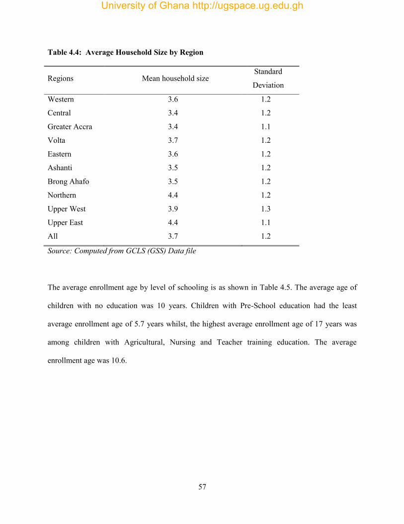
57
Table 4.4: Average Household Size by Region
Regions Mean household size Standard
Deviation
Western 3.6 1.2
Central 3.4 1.2
Greater Accra 3.4 1.1
Volta 3.7 1.2
Eastern 3.6 1.2
Ashanti 3.5 1.2
Brong Ahafo 3.5 1.2
Northern 4.4 1.2
Upper West 3.9 1.3
Upper East 4.4 1.1
All 3.7 1.2
Source: Computed from GCLS (GSS) Data file
The average enrollment age by level of schooling is as shown in Table 4.5. The average age of
children with no education was 10 years. Children with Pre-School education had the least
average enrollment age of 5.7 years whilst, the highest average enrollment age of 17 years was
among children with Agricultural, Nursing and Teacher training education. The average
enrollment age was 10.6.
University of Ghana http://ugspace.ug.edu.gh

58
Table 4.5: Average Enrollment Age by Level of Schooling and Grade Completed
Level of Schooling Mean Standard Deviation
No Education 10.0 3.8
Pre-school 5.7 0.8
Primary 10.1 2.8
Middle/JSS 14.7 1.6
Secondary/SSS 16.3 0.8
Voc/Tech/Commercial Post 16.3 0.9
Sec (Agric/Nursing/Teacher Training 17.0 0.0
All 10.6 3.6
Source: Computed from GCLS (GSS) Data file
Table 4.6 gives a brief description of the percentage distribution of non-working and working
children by school attendance. Out of the proportion of children who are not working, 85.6
percent of them are still attending school. Working children who still attend school constitute
62.7 percent whilst 37.3 percent have never attended school.
Table 4.6: Percentage Distribution of Non-Working and Working Children by
School Attendance
School Attendance Non-working Children (%)
Working Children (%)
Total No. of Children
Never attended school 14.6 37.7 1,497,661
Still attending school 85.4 62.3 4,863,517
Total 100 .0 100.0 6,361,178
Source: Computed from GCLS (GSS) Data file A Chi-square test performed on Table 4.6 gave, 2 (1, N = 6,361,178) = 444,320.143, p < 0.001
(Appendix 1). Since the significance probability quoted is less that critical value of 0.05, there is
a significant association. This is evidence that there is an association between working status of
University of Ghana http://ugspace.ug.edu.gh

59
children and their school attendance in the population in which the sample has been drawn.
Although, there is an association between the two variables, the strength of association is
moderate (Phi and Cramer‟s value V of 0.264) with .001p .
The sex distribution of working and non-working children is represented in Table 4.7. Male
working children are more (53.1%) than their female counterpart (46.9%). There is a similar
proportion of male (53.1%) and female (46.9%) working children.
Table 4.7: Percentage Distribution of Non-Working and Working Children by Sex
Sex Non-working
Children (%) Working
Children (%) Total No. of
Children Male 51.4 53.1 3,313,494
Female 48.6 46.9 3,047,684
Total 100.0 100.0 6,361,178
Source: Computed from GCLS (GSS) Data file
Table 4.7 gave a Pearson Chi-square statistic 2 1680.367 and P < 0.001 (Appendix 1). Hence
there is a very small probability of the observed data under the null hypothesis of no relationship.
The null hypothesis is rejected, since p < 0.05. The sex of the children seems to be related to the
work status. The strength of this association between working and non-working children is
statistically significant but very weak with Phi and Cramer‟s V value of 0.016 at P < 0.001.
The relationship of children to head of household of the working children and non-working is
shown in Table 4.8. The proportion of the son/daughter of head of the household for working
children is (77.4%), whilst “other relative” constitutes the lowest (22.6%). This shows that heads
University of Ghana http://ugspace.ug.edu.gh

60
of households will wish that their children will not work (76.8%) but the prevailing conditions
will force them to do otherwise.
Table 4.8: Percentage Distribution of Non-Working and Working Children by Relationship to Head of Household
Relationship to head of household
Non-working Children (%)
Working Children (%)
Total No. of Children
Son/daughter 76.8 77.4 4,922,720
Other relations 23.2 22.6 1,438,458
Total 100.0 100.0 6,361,178
Source: Computed from GCLS (GSS) Data file.
The percentage distribution of children by age group is represented in Table 4.9. Majority of the
children who are working (48.1%) are in the age group 10-14 years. On the other hand, 53
percent of the non-working children are in the age group 5-9 years. At this age, the children are
very young to engage in any economic activity.
Table 4.9: Percentage Distribution of Non-Working and Working Children by Age Group
Age group of Children age 5-17
Non-working Children (%)
Working Children (%)
Total No. of Children
5-9 53.2 23.7 2,657,285
10-14 34.1 48.1 2,515,490
15-17 12.7 28.2 1,188,403
Total 100.0 100.0 6,361,178
Source: Computed from GCLS (GSS) Data file
A Chi-square test performed on Table 4.9 rejected the null hypothesis of no association between
the working status of the children and the relationship to head of household
University of Ghana http://ugspace.ug.edu.gh

61
[ 2 (2, N= 6,361,178) = 606298.09, p < .000], though there is a moderate relationship between
them, (Phi and Cramer V value = 0.309).
Table 4.10: Percentage Distribution of non-working and working
Children by Size of Household Household Size
Non-working Children (%)
Working Children (%)
Total No. of Children
Less than 3 1.8 1.4 105,418
3-4 16.9 11.4 939,200
5-6 34.0 28.2 2,020,048
7-8 24.5 26.4 1,605,208
9-10 14.9 19.5 1,062,153
Over 10 7.9 13.1 629,152
Total 100.0 100.0 6,361,179
Source: Computed from GCLS (GSS) Data file
Table 4.10 shows the household size for non-working and working children. It is observed that,
the proportion of non-working and working children increases with increasing household size up
to 5-6 and decreases with increasing household sizes. A larger proportion of the working
children (19.2 %) are found in households whose heads are 65 years and over (Table 4.11). A
Chi-square test on the working status of the children and the household size shows a significant
association between them, 2 (5, N= 6,361,179) = 86208.049, p < .000 with moderately weak
strength of association, (Phi and Cramer V value = 0.116).
University of Ghana http://ugspace.ug.edu.gh

62
Table 4.11: Percentage Distribution of Non-Working and
Working Children by Age of Household Head Age of Head of
Household
Non-working
Children (%)
Working
Children (%)
Total No. of
Children
15-34 12.6 7.8 682,105
35-39 15.1 11.1 859,832
40-44 15.9 14.5 978,767
45-49 16.0 15.5 1,007,309
50-54 11.6 14.6 814,128
55-59 7.5 8.3 495,638
60-64 6.9 9.0 491,380
65+ 14.4 19.2 1,032,020
Total 100.0 100.0 6,361,179
Source: Computed from GCLS (GSS) Data file
With regard to literacy (Table 4.12), 66.1 percent of working children were found in households
whose heads are not literate whereas a little above half (51.3%) of the non-working children
came from households whose heads are literate. A further test on the data shown in Table 4.12
gave a Pearson Chi-square statistic, 2 188526.223 at 1df and P < 0.001. This shows a
significant association between the work status of the children and the literacy of their household
heads. Phi and Cramer‟s V value of 0.172 at P < 0.001 shows a moderately weak association
between the two variables. Thus, literate parents tend to prevent their children from working than
those who are not literate.
University of Ghana http://ugspace.ug.edu.gh
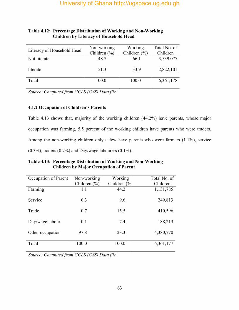
63
Table 4.12: Percentage Distribution of Working and Non-Working Children by Literacy of Household Head
Literacy of Household Head Non-working Children (%)
Working Children (%)
Total No. of Children
Not literate 48.7 66.1 3,539,077
literate 51.3 33.9 2,822,101
Total 100.0 100.0 6,361,178
Source: Computed from GCLS (GSS) Data file
4.1.2 Occupation of Children’s Parents
Table 4.13 shows that, majority of the working children (44.2%) have parents, whose major
occupation was farming, 5.5 percent of the working children have parents who were traders.
Among the non-working children only a few have parents who were farmers (1.1%), service
(0.3%), traders (0.7%) and Day/wage labourers (0.1%).
Table 4.13: Percentage Distribution of Working and Non-Working Children by Major Occupation of Parent
Occupation of Parent Non-working Children (%)
Working Children (%)
Total No. of Children
Farming 1.1 44.2 1,131,785
Service 0.3 9.6 249,813
Trade 0.7 15.5 410,596
Day/wage labour 0.1 7.4 188,213
Other occupation 97.8 23.3 4,380,770
Total 100.0 100.0 6,361,177
Source: Computed from GCLS (GSS) Data file
University of Ghana http://ugspace.ug.edu.gh

64
4.1.3 Education of Parents
The survey solicited information on the highest level of school attended and the highest grade
completed at that level for parents of children age 5-17 years. Education is categorized into: No
Education, Primary, Junior Secondary and Senior Secondary School or higher. The percentage
distribution of non-working and working children by highest level of parents‟ education is shown
in Table 4.14. Twenty eight percent of parents of working children had no education. Of those
children, parents with primary education are very high (52.7%) whilst a small percentage (1.1%)
had a higher level of education.
Table 4.14: Percentage Distribution of Working and Non-Working
Children by Level of Education of Parent Level of Education of Parent
Non-working Children (%)
Working Children (%)
Total No. of Children
No education 11.5 27.6 1,141,040
Primary 71.7 52.7 4,077,353
Junior secondary 14.7 18.6 1,036,681
SSS or higher 2.1 1.1 106,105
Total 100.0 100.0 6,361,179
Source: Computed from GCLS (GSS) Data file
A Chi-square test performed on Table 4.14 gave, 2 (3, N = 6,361,179) = 329128.933, p < 0.000
(Appendix 1). Since the significance probability quoted is less that critical value of 0.05, we
reject the null hypothesis of no association. This is evidence that there is an association between
working status of children and the educational level of their parents in the population in which
the sample was drawn. Although, there is an association between the two variables, the strength
of association is moderate (Phi and Cramer‟s V value of 0.227) with .001p .
University of Ghana http://ugspace.ug.edu.gh

65
4.1.4 Marital status of Parents
For the purpose of this study, marital status has been categorized into married and not married.
The married category comprises married and living together and not married is made up of those
separated, widowed, divorced and single. The distribution of non-working and working children
by marital status of parent is shown in Table 4.15. It can be observed from the results that, when
parents are together, a greater proportion (69.4 percent) of their children do not work. However,
a little more than half (56.5%) of single parents tend to involve their children in economic
activity in other to support the family.
Table 4.15: Percentage Distribution of Working and Non-Working Children by Parent Marital Status
Marital Status of Parent
Non-working Children (%)
Working Children (%)
Total No. of Children
Married 69.4 43.5 3,757,093
Not Married 30.6 56.5 2,604,085
Total 100.0 100.0 6,361,178
Source: Computed from GCLS (GSS) Data file
A Chi-square test performed on Table 4.15 gave, 2 (1, N = 6,361,178) = 424437.429, p < 0.001
(Appendix 1). Hence, the null hypothesis of no association is rejected to p < .000. Although,
there is an association between the two variables, the strength of association is moderate (Phi and
Cramer‟s V value of 0.257) with .001p .
4.1.5 Regional Distribution of Children
Knowledge of the regional distribution of respondents is essential to understanding disparities in
child labour. This is because there is differential resource endowment and behavioral practices in
University of Ghana http://ugspace.ug.edu.gh

66
the regions under consideration. Residents in certain regions are exposed to relatively poor living
conditions and consequently child labour experiences. The percentage distribution of
respondents by region is shown in Table 4.16. Five regions namely Western, Volta, Eastern,
Ashanti and Northern each have over 10 percent of the total working children.
Upper East has the lowest percentage (5%) of working children. Ashanti Region has the highest
percentage (19.0%) of non-working children. This is followed by Greater Accra region (15%),
with Upper West having the lowest percentage (3.7%) of non-working children.
Table 4.16: Percentage Distribution of Working and Non-Working
Children by Region
Region Non-working
Children (%)
Working
Children (%)
Total No. of
Children
Western 8.6 12.4 639,438
Central 8.7 7.3 516,693
Greater Accra 15.2 6.2 747,164
Volta 6.7 10.5 519,006
Eastern 9.8 14.2 733,781
Ashanti 18.7 10.6 988,778
Brong Ahafo 13.4 5.5 657,128
Northern 10.9 18.8 891,096
Upper West 3.7 9.6 381,987
Upper East 4.3 4.8 286,106
All 100.0 100.0 6,361,177
Source: Computed from GCLS (GSS) Data file
University of Ghana http://ugspace.ug.edu.gh

67
4.1.6 Ethnicity Akan (Asante, Fante, and other Akan) are by far the most dominant ethnic group recorded
showing respectively 49.4 percent and 36.3 percent of non-working children and working
children.
Table 4.17: Percentage Distribution of Working and Non-Working Children by Ethnicity Ethnicity Non-working
Children (%)
Working
Children (%)
Total No. of
Children
Akan 49.4 36.3 2,755,586
Ga-Adangbe 7.3 7.8 465,084
Ewe 11.1 12.8 731,690
Guan 4.2 3.2 235,823
Gruma 5.0 10.6 446,851
Mole-Dagbani 16.9 21.4 1,157,985
Grussi 3.0 4.4 219,006
Mande 1.3 2.8 119,814
Other 1.8 0.8 88,717
Total 100.0 100.0 6,220,556
Source: Computed from GCLS (GSS) Data file
The rural-urban distribution of respondents is as shown in Table 4.18. The table reveals that,
79.9 percent of the respondents who are working reside in rural areas whilst 20.1 percent are in
the urban. A little over half (50.6%) of the non-working children were in the rural areas.
A Chi-square test performed this two variables gave, 2 (1, N = 6,361,179) = 559854.28,
p < 0.000 (Appendix 1). This shows significant evidence that there is an association between
working status of children and their locality of residence in the population in which the sample
University of Ghana http://ugspace.ug.edu.gh

68
was drawn. The strength of this association is moderate (Phi and Cramer‟s V value of 0.0.300)
with .001p .
Table 4.18: Percentage Distribution of Working and Non-Working Children by Locality of Residence Locality of Residence
Non-working Children (%)
Working Children (%)
Total No. of Children
Urban 49.4 20.1 2,398,096
Rural 50.6 79.9 3,963,083
Total 100.0 100.0 6,361,179
Source: Computed from GCLS (GSS) Data file
The Percentage distribution of non-working and working children by sex of household head is
presented in Table 4.19. In a male-headed households, about three-quarters (78.4%) of the
children work. On the contrary, majority of the male household heads (72.5%) do not want their
children to work. A Chi-square test performed on the working status of the children and the sex
of head of head of household gave, 2 (1, N = 6,361,177) = 28121.007, p < 0.000 (Appendix 1).
The null hypothesis of no relationship is therefore rejected. Although, there is an association
between the two variables, the strength of association is very weak (Phi and Cramer‟s value of
0.066) with .001p .
Table 4.19: Percentage Distribution of Working and Non-Working
Children by Sex of Head of Household Sex of Head of Household
Non-working Children (%)
Working Children (%)
Total No. of Children
Male 72.5 78.4 4,764,320
Female 27.5 21.6 1,596,857
Total 100.0 100.0 6,361,177
Source: Computed from GCLS (GSS) Data file
University of Ghana http://ugspace.ug.edu.gh

69
Figure 4.1 shows the proportion of children not enrolled in school by age 5 to 17. Generally, the
non-enrolment figure increases from age 6 to age 17 whilst at ages 11 and 16, the non-enrollment
figures decreased.
Source: GCLS, (GSS) Data file Figure 4.1: Children Not Enrolled in School by Age
Figure 4.2 depicts how non-enrolment rates vary by sex of child. This figure shows an opposite
picture of the conventional belief that boys are more likely to be enrolled in school than girls. In
this study, boys‟ non-enrolment rate is higher than that of girls. There is however a drop at age
11 and 16 for both sexes. At age 17, while the non-enrollment rate for girls is almost at the same
level as at age 16, that of boys non-enrollment rate is almost as high as 30 percent. This possibly
reflects the fact that girls may have married or may have withdrawn from school. At the age of
17 boys‟ non enrolment rate is much higher than that of girls.
Pe
rce
nta
ge o
f n
on
-en
rollm
en
t
Age
5 6 7
University of Ghana http://ugspace.ug.edu.gh
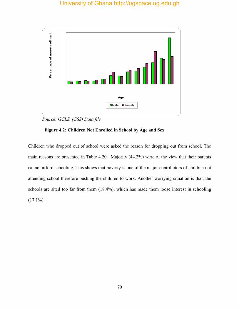
70
Source: GCLS, (GSS) Data file
Figure 4.2: Children Not Enrolled in School by Age and Sex
Children who dropped out of school were asked the reason for dropping out from school. The
main reasons are presented in Table 4.20. Majority (44.2%) were of the view that their parents
cannot afford schooling. This shows that poverty is one of the major contributors of children not
attending school therefore pushing the children to work. Another worrying situation is that, the
schools are sited too far from them (18.4%), which has made them loose interest in schooling
(17.1%).
Perc
en
tag
e o
f n
on
-en
rollm
en
t
Age
Male Female
University of Ghana http://ugspace.ug.edu.gh

71
Table 4.20: Reason for Leaving School
Reason Percent
Parents cannot afford schooling 44.2
School too far away 18.4
Not interested in school 17.1
Family does not allow schooling 5.0
Illness/disabled 2.1
Both parents not alive 0.3
Father not alive 1.3
Mother not alive 1.0
Other reason 10.7
Total 100.0
Source: GCLS (GSS) Data file
4.1.7 Measurement of Children’s Work
The survey asked questions about the occupation of all household members. To classify
children‟s activities, however, we focused on the occupation of children reported by household
heads. Work was defined broadly to include non-wage work and housework.
Two occupations (primary and secondary) were considered as the key indicators of child work.
Work and study are not mutually exclusive as the data suggests, some children reported
attending school, while at the same time performing some form of paid or unpaid work. Thus,
four mutually exclusive categories are created to define child‟s activity. These categories are;
study only, work only, work and study, neither work nor study. Children are classified into
University of Ghana http://ugspace.ug.edu.gh

72
“study only category”, if their primary and secondary occupation is student or they do not have a
secondary occupation. Similarly, “work only” category includes those children whose primary
and secondary occupation is work or they do not have any secondary occupation. Children who
work and attend school as well are included in “work and study” category. Neither “work nor
study” category considers those who are reported as children but not in a position to work or go
to school although they are of school going age.
Figure 4.3 shows that 5.5 percent of children attended school (study) as their only activity. A
smaller percent of the children were engaged in work only (0.5%) whilst 89.7 percent combines
study with work.
Source: Computed from GCLS Data file
Figure 4.3: Distribution of Children by Activity Status
0.5 5.5
89.7
4.3
0
10
20
30
40
50
60
70
80
90
100
work only attending schoolonly
working andattending school
neither workingnor attending
school
University of Ghana http://ugspace.ug.edu.gh

73
4.1.8 Activity Status of Children Table 4.21 represents activity status of children by sex and age. The data shows that there are
some children who begin to work from 5 years of age. The proportion of children in the “work
only” category increases with age, particularly, from 12 years to 17 years. Generally, an
overwhelming majority (91.9% boys and 87.3% girls) of children study and work at the same
time.
Table 4.21: Activity Status of Children by Sex and Age
Activity Status
Study only Work and Study Work only
Neither
Total
Number of Children
Sex
Boys
4.6
91.9
0.3
3.2
100.0
3,313,494
Girls
6.5
87.3
0.7
5.5
100.0
3,047,685
All
5.5
89.7
0.5
4.3
100.0
6,361,179
Age
5
1.5
94.7
0.0
3.8
100.0
481,517
6
2.4
94.2
0.1
3.3
100.0
553,646
7
2.5
93.7
0.1
3.7
100.0
573,875
8
3.8
92.7
0.1
3.5
100.0
541,495
9
3.5
91.6
0.4
4.5
100.0
506,752
10
5.4
89.7
0.2
4.7
100.0
596,769
11
7.7
86.6
0.1
5.6
100.0
429,827
12
6.1
88.0
0.6
5.2
100.0
577,183
University of Ghana http://ugspace.ug.edu.gh

74
13
7.4
88.1
0.6
3.9
100.0
465,577
14
7.4
87.4
0.8
4.4
100.0
446,138
15
7.9
86.6
1.2
4.3
100.0
513,131
16
11.7
82.8
1.0
4.5
100.0
371,608
17
8.8
84.7
2.0
4.6
100.0
303,664
All
5.5
89.7
0.5
4.3
100.0
6,361,179
Source: Computed from GCLS (GSS) Data file
University of Ghana http://ugspace.ug.edu.gh
75
4.2 FURTHER ANALYSIS
4.2.0 Introduction
Bivariate logistic regression and multilevel techniques are used to assess differentials in child
labour and schooling. The aim here is to determine whether the observed pattern in child labour
and schooling varies significantly among categories of a given variable.
Logistic regression is one of the analytical methods employed in this study. A major component
of this study is the analysis of the various differentials in child labour and schooling. To identify
the important factors affecting child labour, a logistic regression model, which allows the
assessment of the relative influence of each variable, is used. The odds of a child labour can be
evaluated using the standard logit model.
In the multilevel analysis, the children in the various households are examined to see the
influence their respective households can have to let a child school and work at the same time or
school without working while correcting for association within households. The children in the
households are regarded as level one unit and the households as level two units. The various
predictors that may cause a child to engage in economic activity were examined within the
various households.
The following are used as predictors in this analysis; age of head of household, gender of head of
household, marital status of parents, father‟s occupation, mother‟s occupation, relationship to
head of household, residing in rural/urban area, literacy of head of household, sex of the child
and highest educational level attained with the schooling and working status of the child being
the response variable.
University of Ghana http://ugspace.ug.edu.gh

76
The statistical software used in the analysis of the multilevel differentials and to estimate the
'i s in the regression model is the Statistical Package for the Social Science, SPSS (SPSS Inc.,
1988).
In SPSS, the parameters of the logistic regression model are estimated using the maximum-
likelihood method. SPSS employs two main approaches to assess the goodness of fit. These are
the Wald test and the Likelihood Ratio Test for two nested models. The unit of analysis in this
chapter is the children aged 5-17 years. The variables included in the logistic regression as well
as their estimated coefficients, standard errors, significant values, odds ratio and confidence
intervals are reported in Table 4.26.
4.2.1 Findings
In the main analysis (Table 4.26), the work and school status (a child working and schooling at
the same time or schooling only) was used as dependent variable and the variable taking value 1
if the child is reported schooling and working or 0 if the child reported schooling only.
.
4.2.2 Model for children’s schooling and working using logistic regression
Logistic regression compares the null model (model without the coefficients) with a model
including all the predictors to determine whether the latter model is more appropriate. The
classification table for the null model suggests that if we knew nothing about our variables and
guessed that a child would attend school and work, we would be 86.1 percent correct of the time.
This table describes the baseline model (Appendix 1),
University of Ghana http://ugspace.ug.edu.gh

77
The Omnibus Tests of Model Coefficients (Table 4.22) is used to check that the new model (with
explanatory variables included) is an improvement over the baseline model. It uses chi-square
tests to see if there is a significant difference between the Log-likelihoods (-2LLs) of the baseline
model and the new model. If the new model has a significantly reduced -2LL compared to the
baseline then it suggests that the new model is explaining more of the variance in the outcome
and is an improvement. The chi-square is highly significant (chi-square =1900671.06, df = 23,
p<.001) so the new model is significantly better.
Source: Computed from GCLS Data File. The Model Summary (Table 4.23) provides the -2LL and pseudo-R2 values for the full model.
The -2LL value for this model (3226822.9) is what was compared to the -2LL for the previous
null model in the “omnibus test of model coefficients” which shows that there was a significant
decrease in the -2LL. That is, the new model (with explanatory variables) is significantly better
fit than the null model. The R2 values gives approximately how much variation in the outcome is
explained by the model. The Nagelkerke‟s R2 suggests that the model explains roughly 46.7% of
the variation in the outcome. Both Nagelkerke‟s and Cox & Snell R square give different values
which are all approximations but Nagelkerke‟s R2 is more robust.
Table 4.23 Model Summary Step -2 Log
likelihood Cox & Snell R
Square Nagelkerke R Square
1 3226822.932 .258 .467 Source: Computed from GCLS Data File.
Table 4.22 Omnibus Tests of Model Coefficients Chi-square df Sig.
Step 1 Step 1900671.059 23 .000 Block 1900671.059 23 .000 Model 1900671.059 23 .000
University of Ghana http://ugspace.ug.edu.gh

78
Table 4.24 shows that the full model correctly classifies 90.0% of the model as compared to
86.1% in the null model. This means that, by adding the variables, we can now predict with
90.0% accuracy. Thus the model correctly fits the data.
Table 4.24 Classification Table for Binary Logistic Regression
Observed
Predicted Attending school and working Percentage
Correct Attending school and
work
Schooling only
Attending school and working
Attending school and work 5335748 141623 97.4 Schooling only 491960 391847 44.3
Overall Percentage 90.0 Source: Computed from GCLS Data File. Table 4.25 provides the regression coefficient ( ), the Wald statistic, to test the statistical
significance of the model and if the significance level is less than 0.05, we reject the null
hypothesis and accept the alternative hypothesis. Where the null and the alternate hypothesis
states that;
: , Xi makes no significant contribution in the model
: Xi makes a significant contribution in the model.
Estimates from Table 4.25 shows that all the predictors of interest (Xi‟s) are all significant at
p < .000. Hence we reject the null hypothesis and conclude that the predictors make significant
contribution in the model.
University of Ghana http://ugspace.ug.edu.gh
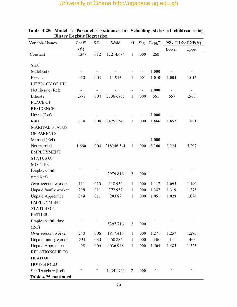
79
Table 4.25: Model 1: Parameter Estimates for Schooling status of children using Binary Logistic Regression
Variable Names Coeff. ( )
S.E. Wald df Sig. Exp( ) 95% C.I.for EXP( ) Lower Upper
Constant -1.348 .012 12214.684 1 .000 .260
SEX Male(Ref) - - - - - 1.000 - -
Female .010 .003 11.913 1 .001 1.010 1.004 1.016 LITERACY OF HH Not literate (Ref) - - - - - 1.000 - - Literate -.579 .004 23367.865 1 .000 .561 .557 .565 PLACE OF RESIDENCE
Urban (Ref) - - - - - 1.000 - - Rural .624 .004 24751.547 1 .000 1.866 1.852 1.881 MARITAL STATUS OF PARENTS
Married (Ref) - - - - - 1.000 - - Not married 1.660 .004 218246.341 1 .000 5.260 5.224 5.297 EMPLOYMENT STATUS OF MOTHER
Employed full time(Ref)
- - 2979.816 3 .000
- -
Own account worker .111 .010 118.939 1 .000 1.117 1.095 1.140
Unpaid family worker .298 .011 772.957 1 .000 1.347 1.319 1.375 Unpaid Apprentice .049 .011 20.089 1 .000 1.051 1.028 1.074 EMPLOYMENT STATUS OF FATHER
Employed full time (Ref)
- - 5397.716 3 .000
- - -
Own account worker .240 .006 1817.416 1 .000 1.271 1.257 1.285 Unpaid family worker -.831 .030 750.884 1 .000 .436 .411 .462 Unpaid Apprentice .408 .006 4036.948 1 .000 1.504 1.485 1.523 RELATIONSHIP TO HEAD OF HOUSEHOLD
Son/Daughter (Ref) - - 14341.723 2 .000 - - -
Table 4.25 continued
University of Ghana http://ugspace.ug.edu.gh

80
Variable Names Coeff. ( )
S.E. Wald df Sig. Exp( ) 95% C.I.for EXP( ) Lower Upper
Other Children .391 .005 6139.251 1 .000 1.479 1.465 1.494 AGE OF HEAD OF HOUSEHOLD
15 – 34 (Ref) - - 9002.021 7 .000 - - -
35 – 39 -.026 .007 15.502 1 .000 .974 .962 .987 40 – 44 .047 .006 53.802 1 .000 1.048 1.035 1.062 45 – 49 .296 .006 2244.210 1 .000 1.344 1.328 1.361 50 – 54 .299 .006 2215.788 1 .000 1.349 1.332 1.366 55 – 59 .225 .007 988.610 1 .000 1.252 1.235 1.270 60 – 64 .343 .007 2387.346 1 .000 1.409 1.390 1.429 65+ .043 .006 47.078 1 .000 1.044 1.031 1.057 GENDER OF HOUSEHOLD HEAD
Male (Ref) - - - - - 1.000 - - Female -.119 .004 839.366 1 .000 .888 .880 .895 EDUCATIONAL LEVEL OF PARENTS
No Education (Ref) - - 853540.037 3 .000 - - -
At most Primary -3.298 .004 804850.888 1 .000 .037 .037 .037 Junior Secondary -3.072 .005 382365.947 1 .000 .046 .046 .047 SSS or Higher -2.839 .012 57692.449 1 .000 .059 .057 .060
(The reference category is Attending School & working) Source: Computed from GCLS Data File.
4.2.3 Characteristics of Children
Child characteristics, such as sex and relationship to household head appear to be important
determinants of whether or not children attend school and work. The sex coefficient has a
positive effect on the probability of attending school and working. Female children are more
likely to attend school and work as compared to male children and the odds of attending school
and working is 1.010. This suggests that female children are 1.010 times as likely to be classified
University of Ghana http://ugspace.ug.edu.gh

81
as attending school and working as male children holding constant the other independent
variables.
Table 4.25 indicates that if a child is not the son or daughter of the head of household, then the
probability of attending school and working is moderately high. The odds of attending school
and working of other relations are 1.465 (or 46.5%) times as likely as that of a child of the head
of household. This coefficient shows significant positive effect on the probability of attending
school and working. This implies that household heads favour their own children by preventing
them from attending school and working at the same time.
4.2.4 Characteristics of Parents
All the parental characteristics namely, highest education level of parents, marital status of
parent, literacy of parent and employment status of both father and mother are all statistically
significant. The literacy of parents has negative effect on the probability of attending school and
work. For example, the odds ratio for a literate parent is 0.561. This suggests that children of
literate parents‟ are 0.561 times as likely to attend school and work as children of illiterate parent
holding constant the other independent variables. The marital status of the parents has a great
impact on whether or not a child attends school and work. The odds ratio of a single parent (not
married) is 5.26. This suggests that children from single parents are 5.260 times as likely to
attend school and work as children whose parents are still married holding all other variables
constant.
Both father‟s and mother‟s employment status have significant impact on the probability of a
child “attending school and working”. The odds ratio of unpaid family worker of the
University of Ghana http://ugspace.ug.edu.gh

82
employment status of mother is 1.347. This shows that if a child‟s mother is an unpaid family
worker, that child is 1.347 times (or about 35%) more likely to attend school and work than those
whose parents are in full time employment.
On the other hand, own account worker of the employment status of father indicate that, their
children are as likely to attend school and work. The odds ratio is 1.257. Again, children whose
father is an unpaid apprentice are 50.4% (OR = 1.504) more likely to attend school and work
than those whose father is in full time employment.
Highest educational level of the parents significantly contributes to a child schooling or working.
A parent who has attained either SSS or higher education is less likely than a parent who has no
education to let his/her child attend school and work (OR = 0.056). A parent whose highest
education is Junior Secondary has odds ratio of 0.046 while a parent with at most primary
education has odds ratio of 0.037. This shows that increasing the educational level of parents
tends to decrease the likelihood of his/her child schooling and working.
4.2.5 Characteristics of Household
Among the household characteristics, age of household head and gender of household head are
all statistical significant. The age of head of household plays an important role as to either a child
should attend school and work or not. It is shown from Table 4.25 that, the odds ratio of children
living with age group of household head, 45 - 49 and 50 - 59 are respectively about 34%
(OR = 1.344) and 35% (OR = 1.349) more likely to let their children attend school and work as
those aged 15 – 34 years. A child is more likely to attend school and work (OR = 1.409) when
the head of his/her household reaches the pension age (60 – 65 years). This notwithstanding,
University of Ghana http://ugspace.ug.edu.gh

83
younger household heads (35 – 39 years) are less likely (OR = 0.974). Children of female headed
household children are less likely to attend school and work as children to a male headed
household (OR = 0.888).
Another socio-economic variable, which is significant, as an independent determinant of children
attending school and working, is the type of place of residence. The analysis shows that children
living in the rural areas are 1.822 (82.2%) times as likely to attend school and work as those in
the urban areas.
4.2.6 Multilevel analysis
The reason for this analysis is that, information from children coming from the same household
are not independent. Using the logistic regression may under-estimate the precision of the
estimates. Hence, a cluster-specific model may be appropriate.
The children in the various households are examined to see the effect these households can have
on a child schooling and working at the same time using multilevel logistic regression. The
children in the households are regarded as level one unit and the households as level two units.
The various predictors that may cause a child to school and work were examined within the
various households. All the predictors used in the binary Logistic are also used in this analysis.
Table 4.28 shows that the households significantly affect the children to attend school and work
since all are statistically significant except the household head whose age is between 35 and 39
years.
University of Ghana http://ugspace.ug.edu.gh

84
Table 4.26 gives the observed and predicted values for the null model using multilevel logistic
regression. This shows that if we knew nothing about the model and decide to guess, we will be
62.1% correct of predicting children who are only attending school and 98.1% of those who
combines school and work with overall correct prediction of the model as 93.1%.
Table 4.26 Classification table for the Intercept only model
Observed Predicted
Schooling Attending school and work
Schooling only Percent
62.1%
37.9%
Attending school and work
Percent
1.9%
98.1%
Overall Percent correct 93.1%
Source: Computed from GCLS Data File
When all the predictors are added, the model (Table 4.27) was able to predict correctly 87.2% of
children who are only attending school and 98.5% of those who are combining school and work.
The model gave the overall correct percentage as 96.9%. The overall performance of the model
using logistic regression was predicted as 90.0%. These predictions depict that the average
performance of the multilevel logistic model fits the data better than the binary logistic model.
Table 4.27 Classification for the full model
Observed Predicted
Schooling Attending school and work
Schooling only Percent count
87.2% 770,051
12.8% 113,491
Attending school and work
Percent count
1.5% 84,251
98.5% 5,391,706
Overall Percent correct 96.9%
Source: Computed from GCLS Data File
University of Ghana http://ugspace.ug.edu.gh
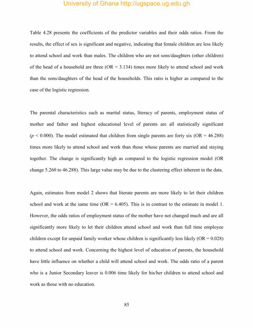
85
Table 4.28 presents the coefficients of the predictor variables and their odds ratios. From the
results, the effect of sex is significant and negative, indicating that female children are less likely
to attend school and work than males. The children who are not sons/daughters (other children)
of the head of a household are three (OR = 3.134) times more likely to attend school and work
than the sons/daughters of the head of the households. This ratio is higher as compared to the
case of the logistic regression.
The parental characteristics such as marital status, literacy of parents, employment status of
mother and father and highest educational level of parents are all statistically significant
(p < 0.000). The model estimated that children from single parents are forty six (OR = 46.288)
times more likely to attend school and work than those whose parents are married and staying
together. The change is significantly high as compared to the logistic regression model (OR
change 5.260 to 46.288). This large value may be due to the clustering effect inherent in the data.
Again, estimates from model 2 shows that literate parents are more likely to let their children
school and work at the same time (OR = 6.405). This is in contrast to the estimate in model 1.
However, the odds ratios of employment status of the mother have not changed much and are all
significantly more likely to let their children attend school and work than full time employee
children except for unpaid family worker whose children is significantly less likely (OR = 0.028)
to attend school and work. Concerning the highest level of education of parents, the household
have little influence on whether a child will attend school and work. The odds ratio of a parent
who is a Junior Secondary leaver is 0.006 time likely for his/her children to attend school and
work as those with no education.
University of Ghana http://ugspace.ug.edu.gh
86
The ages of head of households are all significant at p < 0.001 except age group of 35 – 39 years.
Age group of head of household between 55 – 59 years are seventy one (OR = 71.194) times
more likely for their children to school and work at the same time. The same can be said for
those between 45 – 49 years. Their children are 18.783 times more likely to attend school and
work as those between 15 – 34 years controlling all other predictors. The odds of a female of a
female headed household has not changed much (OR change 0.888 to 0.716) and they are all less
likely to attend school and work as their male counterpart. The differences in odds ratio
compared may be explained by the random effect imbedded in the multilevel logistic model.
Table 4.28 Model 2: Parameter Estimates for Schooling status of children using Multilevel Logistic Regression
Variable Names Coeff.(B) Sig. Exp(B)
Constant -9.995 .000 0.000
SEX Male(Ref) - - 1.000
Female -0.110 .000 0.896 LITERACY OF HH Not literate (Ref) - - 1.000 Literate 1.858 .000 6.405 PLACE OF RESIDENCE Urban (Ref) - - 1.000 Rural 3.128 .000 22.834 MARITAL STATUS OF PARENTS
Married (Ref) - - 1.000 Not married 3.835 .000 46.288 EMPLOYMENT STATUS OF MOTHER
Employed full time(Ref) - .000 1.000
Own account worker 0.427 .000 1.532 Unpaid family worker 0.323 .000 1.382 Unpaid Apprentice 0.813 .000 2.255 EMPLOYMENT STATUS OF FATHER
Employed full time (Ref) - .000 1.000
University of Ghana http://ugspace.ug.edu.gh

87
Table 4.28 continued Variable Names Coeff.(B) Sig. Exp(B)
Own account worker 0.385 .000 1.470 Unpaid family worker -0.385 .000 0.028 Unpaid Apprentice 0.205 .000 1.679 RELATIONSHIP TO HEAD OF HOUSEHOLD
Son/Daughter (Ref) - .000 1.000
Other Children 1.143 .000 3.134 AGE OF HEAD OF HOUSEHOLD
15 – 34 (Ref) - .000 1.000
35 – 39 -0.119 .124 0.888 40 – 44 -0.538 .000 0.584 45 – 49 2.933 .000 18.783 50 – 54 0.959 .000 2.610 55 – 59 4.265 .000 71.194 60 – 64 1.404 .000 4.070 65+ 1.3.3 .000 3.680 GENDER OF HOUSEHOLD HEAD
Male (Ref) - - 1.000 Female -0.334 .000 0.716 EDUCATIONAL LEVEL OF PARENTS
No Education (Ref) - .000 -
At most Primary -5.601 .000 0.004 Junior Secondary -5.136 .000 0.006 SSS or Higher -3.476 .000 0.031
(The reference category is Attending School & working) Source: Computed from GCLS Data File. The covariance of the random effects between the children and the households for the baseline
model is displayed in Table 4.29. When no predictor has been entered at level one, there is still a
significant variability between the children and the households. (Wald Z = 460626, p < .000).
University of Ghana http://ugspace.ug.edu.gh

88
Table 4.29 Covariance Parameters for the null model 95% Confidence
Interval
Random Effect Block
Estimate(B) Std. Error
Z Sig. Lower Upper
Var(intercept) 26.556 0.570 460626 .000 26.463 27.696
Source: Computed from GCLS Data File. Table 4.30 again shows the estimates of the random effects that exist between the children level
and the household level. The inclusion of the predictors of interest to the model significantly
increased the variability between these levels.
Table 4.30 Covariance Parameters for the full model (model 2) 95% Confidence
Interval
Random Effect Block
Estimate(B) Std. Error
Z Sig. Lower Upper
Var(intercept) 33.900 0.809 41.887 .000 32.350 35.524
Source: Computed from GCLS Data File
University of Ghana http://ugspace.ug.edu.gh

89
CHAPTER FIVE
SUMMARY, DISCUSSIONS, CONCLUSIONS AND RECOMMENDATIONS
This chapter presents summary of the findings from the study, and recommends rational measures
for government, stockholders and those in child care. It again recommends
5.1 Summary
The objectives of the study were to establish the relationship of child labour and schooling, to
determine socio-economic factors affecting child labour and schooling and make
recommendations, based on the findings, for appropriate intervention measures to further reduce
this menace.
The 2003 GCLS data was the main source of data used for the analysis. The target population
was children aged 5-17. This study has examined the relationship between selected socio-
economic variables influencing child labour and schooling in Ghana. These variables are
parents‟ educational level, major occupation of parent, type of place of residence, region and
place of residence, marital status, employment status of mother and father, relationship to the
head of household, age of the head of household, sex of the head of household, literacy of parent,
religious affiliation and ethnic group.
The examination of the determinants of child labour in Ghana was done using bivariate and
multivariable techniques. In the bivariate analysis, children working and not working were
applied to all the variables already stated. In multivariable analysis, logistic regression and
University of Ghana http://ugspace.ug.edu.gh

90
multilevel logistic regression were applied to children aged 5-17 years old who were attending
school. Further, the multilevel analysis was used to correct for within-household association.
Empirical results show that if the parent was employed in a vulnerable occupation, for example,
day-labour or wage-labour, it raises the probability of the child attending school and work.
Most of the children in the study are engaged in household work that allows them to attend
school and work because household work is more flexible than formal or informal wage earning
jobs. Another interesting finding of this study is that boys‟ non-enrollment rate is higher than
girls‟ in some ages.
It was also found out that children who are the sons and daughters of the head of household are
less likely to attend school and work as the other relations. This may reflect the fact that if the
household head is resource constrained then it is likely for him to choose first his own child for
schooling. This finding further threw light on the relationship of child labour and poverty.
The expected results indicate that children whose parents are traders and unpaid family workers
are likely to attend school and work; the reason being that parents‟ income level cannot afford to
carter for the entire household without their children supplementing it. Again, the likelihood of a
child from a single parent to attend school and work is very high.
It was again found out that, households influence their respective children to attend school and
work at the same time. If a child will engage in any economic activity, it will depend largely on
the household in which he/she lives. Engaging in economic activity also affects the education of
the child involved.
University of Ghana http://ugspace.ug.edu.gh

91
Even though the study attempted to control the effects of socio-economic variables in order to
assess the proper effect of work on their health and psychosocial status, the attempt might not
have succeeded fully because of the differences between the socio-economic status of children
may be variable within the same group. Also socio-economic variables may have a profound
effect on both the health outcomes and on the work status of children at the same time making it
difficult to disentangle their separate effects.
5.1.1 Limitations of the study
Data is a major obstacle in carrying out child labour research. Most studies suffer from difficulty
in obtaining reliable child labour data. Reasons for this are, firstly, there is difficulty in reaching
households with child labour, and even if they are questioned, stigma and illegality of child
labour prompts them to deny its existence.
Secondly, the survey relies on the recall memory of parents, so it is possible that there has been
systematic under-reporting of some work-related and family socio-economic characteristics. It is
impossible to verify such details in a survey of this nature and some caution should be exercised
in interpreting the results.
Another difficulty when collecting information in rain fed regions is migration. In dry seasons,
especially in villages with no functional irrigation facilities, many households migrate to more
water rich regions as agricultural labourers, or to cities for other jobs such as construction works.
Depending on duration, migrant families sometimes take their children with them.
University of Ghana http://ugspace.ug.edu.gh

92
Although the survey attempted to identify a representative sample of working children, it is
likely that the sample does not fully represent the extent of child labour since many working
children are engaged in domestic and invisible activities. This may form an obstacle to the
generalization of results to the whole of country.
5.1.2 Study strengths
The study has a number of strengths, which lend support to the plausibility of its findings. Strong
associations were observed in relation to the main objectives of the study. The results reported in
this study were also consistent with those previously published by a number of different
researchers using different methodologies
A clear definition of child labour was employed which made the sampling procedure easier and
more accurate. The study area chosen has a wide range of different types of community, both
rural and urban with a fair geographical spread, and a wide variety of economic activities. Thus,
it might provide a realistic indicator of the national status of child labour allowing generalization
of the results to the country as a whole.
5.2 Discussions
One of the aims of this study was to find out the various factors which influence children aged
5-17 years to engage in various kinds of economic activities while schooling. Following from the
data collected, it emerged that one of the main reasons why children engage in economic activity
while schooling was to help supplement their parents‟ income. Thus, when parents are
financially sound the child‟s needs could easily be met.
University of Ghana http://ugspace.ug.edu.gh

93
The findings of the study showed that both working and non-working children came from large
families with household size between 3- 4 and 5 - 6. It then decreases from household size of
7 - 8, 9 - 10 and higher than 10 (Table 4.10). This confirms the finding of Becker who said that a
household with many potential workers, the probability that a child will attend school and work
is somewhat lower (Becker, 1993).
According to the study, a son or a daughter of head of household was being favoured in terms of
attending school and work. So it is not surprising that the other relations have the higher
probability of attending school and work than that of the sons or daughters of the head of
household.
Although this study could not provide any specific direction on the dependency of child labour
and household welfare, it tries, however, to indicate that child labour is negatively related with
household income and welfare that is proxied by both the occupation and status of employment
of parents.
The study reveals that children who combine school with work could be found in all the year
groups 5-9, 10-14 and 15-17, even though it is higher in the age group 5-9 (63.7%) and age
group 10-14 (71.0%). A number of children combining schooling with work in the age group 15-
17 constitute (53.0%). A significant number of children (90%) attend school and work at the
same time. It follows that many children are combining schooling with various income earning
activities, perhaps because the trade is very lucrative or simply to supplement effort of guardian
in catering for their schooling.
University of Ghana http://ugspace.ug.edu.gh

94
5.3 Conclusions
In assessing the socio-economic determinants of child labour and schooling in Ghana, logistic
regression was applied to the variables in order to capture the predictor of child labour and
schooling. These analyses have assisted in identifying the significant variables; sex, relationship
to head of household, age group, major occupation of parent, literacy of parent, employment
status of father, residency and religion associated with the child working and attending school.
The most significant findings from this study are that, male children are as likely to attend school
and work as female. In spite of the fact that 15-17 years of age is a typical school going age, in
the case of the group that was studied, it came out that, the 15-17 year group combined school
with work.
The result indicates that, children combined school with work as a result of their relationship to
the head of household. This time the emphasis is on the nuclear family and not the extended
family.
Children who combined school with work tend to be in a household with the major occupation of
parent being “other” occupation, unpaid apprentice and also lived in the rural areas because
many of the rural dwellers are not financially sound and they will need their children to work to
supplement the household. These children are likely to come from parents who are not literate.
University of Ghana http://ugspace.ug.edu.gh

95
5.4 Recommendations
The results of the study and the literature show that the problem of child labour is extensive and
there is an urgent need for action. Ghana, in common with most developing countries, is not
financially and institutionally prepared to put an end to the phenomenon at once as child labour
and poverty are intertwined and the earnings of working children are essential for their families'
survival. Therefore, the most logical and acceptable strategy in the country could be to focus on
the eradication of the most intolerable forms of child labour and the protection from hazardous
occupations, exploitation and abuse of those, especially the very young, who continue to be
economically active.
The problem related to the size and nature of child labour should be addressed. Working children
are usually engaged in invisible hazardous work, which is likely to affect their education and
endanger their health. To achieve visibility, a national survey should be carried out as soon as
possible forming an essential point of departure for any action for elimination or at least
decreasing the incidence of hazardous work among children.
Theoretically education is compulsory in the country up to Junior High School level but
unfortunately the situation in practice is different. Drop out from school by working children is
quite common and usually no action is taken. This is because some parents may lack faith in
education and consequently they encourage their children to leave school and engage in work
while these children can learn skills and gain experience for the future. Drop out from school
may be due to the difficult economic status of parents who cannot afford the expense of their
children's education. More attention should be paid to children of less literate and poor parents
(estimated by occupation) as they cannot afford schooling
University of Ghana http://ugspace.ug.edu.gh

96
In Ghana, the enforcement of law and the improvement of education alone are unlikely to
eradicate child labour. Simply making schools available and improving their quality will not be
sufficient to overcome all the problems faced by the poorest families in the quest to send their
children to school. The hard economic condition of the families and the high rate of
unemployment among the people force them to send their children to work. Child labour cannot
be eliminated without action to address poverty.
One of the important conclusions that can be drawn from this study is that, if there is no
conscious effort of the Ghana Education Service to encourage girls to attend school, then those
girls who are combining school and work would move into working instead of schooling.
Moreover, appropriate policy can shift children who are both attending school and working
toward schooling as their only activity. Hence, the government of Ghana should continue with a
program that will encourage children all over the country to attend school while more focus
should be given to its proper and fruitful implementation.
University of Ghana http://ugspace.ug.edu.gh

97
REFERENCES
Acquah, L. (1972). A social survey of the capital of Ghana, formerly called the Gold Coast,
Undertaken FO. Accra: Ghana University Press.
Addison, T., Bhalotra, S., Coulter, F., and Heady, C., (1997). Child labour: A Preliminary view.
Centre for Development Studies. England: University of Bath Claverton Down.
Afenyadu, D. (2008). Children in Cattle Herding: A Baseline Study of the North and South
Tongu Districts commissioned by the International Needs Network Ghana
(unpublished paper).
Agresti, A. (1996). An Introduction to Categorical Data Analysis. New York: Wiley.
Ashagrie, K. (1997). Methodological child labour surveys and statistics. Bureau of Statistics and
International Programme on the Elimination of Child labour. Geneva: ILO.
Aitkin, M., Anderson, D., Brian, F., & Hinde, J. (1989). Statistical modelling in GLIM. Oxford:
Oxford University Press.
Asogwa, S. (1986). Socio-medical Aspects of Child Labour in Nigeria. Journal of Occupation
Medicine, 28: 46-48.
Akabayashi, H., and Psacharopoulos, G. (1999). The Trade-off Between Child Labor and Human
Capital: A Tanzanian Case, Journal of Development Studies, 35(5): 120-140.
Baland, J., and J. Robinson (2000). Is Child Labor Inefficient?, Journal of Political Economy,
108:663-679.
Banerjee, S. R. (1995). Child labor in India: Present status. Indian Pediatrics, 32: 403 - 408.
Basu, K. (1999). Child Labor: Cause, Consequence, and Cure with Remarks on
International Labor Standards, Journal of Economic Literature, 37: 1083-1119.
University of Ghana http://ugspace.ug.edu.gh

98
Becker, G. S. (1965). A theory of the allocation of time. Economic Journal, 75, 493 - 517.
Becker, G.S. (1993). Nobel lecture: The economic way of looking at behaviour. Journal of
Political Economy, 101, 385-409.
Becker, G. S., & Lewis, H. G. (1973). On the interaction between the quantity and quality of
children. Journal of Political Economy, 81(2), Part 2, S279-S288.
Beegle, K., Dehejia, R., and Gatti, R. (2006). Child Labor and agricultural shocks,
Journal of Development Economics, vol 81(1): 80-96.
Black, M. (1986). The children and the nations: The story of Unicef. New York: Unicef.
Blanchard, F.(1983). Report of the Directory-General. Geneva: ILO.
Boozer, A., Michael, A., and Suri, K. (2001). Child Labor and Schooling Decisions in Ghana.
Unpublished manuscript.
Busia, K. (1950). Report on Social Survey of Sekondi-Takoradi, Crown Agents. London.
Cain, M. T. (1977). The economic Activities of Children in a Village in Bangladesh. Population
and Development Review, 3(3): 201-227.
Cavalieri, C. (2002). The Impact of Child Labor on Educational Performance: An Evaluation of
Brazil. Manuscript
Cockburn, J. (2000). Child Labour Versus Education: Poverty Constraints or Income
Opportunities? Unpublished manuscript.
Cockburn, J., and Benoit, D. (2007). Child Work and Schooling: The Role of Household Asset
Profiles and Poverty in Rural Ethiopia. Journal of African Economies. 16(4): 519-
63.
Damodaran, A. (1997). The working children and the street child: effect on the future child
development. Bulletin of the New York Academy of Medicine, 74(1): 81-89.
University of Ghana http://ugspace.ug.edu.gh
99
Denuit, M. Bourher, P., and Guillen, M. (2007). Actuarial Modelling of Claim Counts: Risk
Classification, Credibility and Bonus-MalusSystems. Chichester: John Wiley &
Sons Ltd.
De Tray, D. N. (1973). Child quality and the demand for children. Journal of Political
Economy, 81, S70-S95.
Dunn, Kathleen, A., Carol W., Lisa R., and Michael, D. (1998). Teens at Work: A Statewide
Study of Jobs, Hazards, and Injuries. Journal of Adolescent Health. 22(1): 19- 25.
Duraisamy, M. (2000). Child schooling and child work in India, Paper presented at the Eighth
World Congress of the Econometric Society. August 11-16.
Dustmann, C., Micklewright, N., and Smith, S. (1996). Earning and learning: educational policy
and the growth of part-time work by fulltime pupils, Fiscal Studies, 17(1): 79-103.
Edmonds, Eric and Pavcnik, N. (2002). Does Globalization Increase Child Labor? Evidence
from Vietnam. NBER Working Paper No. 8760.
Emerson, P. M., & Portela, A. (2001). Bargaining over sons and daughters: Child labor, school
attendance and intra-household gender bias in Brazil. Working paper. Denver:
University of Colorado.
Emerson, P. M., and Shawn, D. K. (2006). Opportunity, Inequality, and the Intergenerational
Transmission of Child Labor. Economica. 73(291): 413-434.
Estrella, G. (1994). Case Studies on Hazardous Child Labour. International Child Health: a
digest of current information, 2: 61-72.
Fortes, M. (1949). The web of kinship among the Tallens: The second part of an analysis of the
social structure. London: Oxford University Press.
Geyer, C. J. (2003, September 30). Maximum Likelihood. Maximum Likelihood in R, pp. 1 – 9.
University of Ghana http://ugspace.ug.edu.gh

100
Ghana Education Acts 1961 (Act 87). Labour Laws Journal of Adult and Youth Education 1949-
64.
Ghana Statistical Service. (2003). Ghana child labour survey. Accra: Ghana Statistical Service.
Ghana Statistical Service. (2006). Multiple Indicator Cluster Survey. Accra: Ghana Statistical
Service.
Glonek, G.F.V., and McCullagh, P. (1995) Multivariate logistic models. Journal of the Royal
Statistical Society, Series B, 81, 477–482.
Graitcer, P., and Lerer, L. (1998). Child Labor and Health: Quantifying the global health
impacts of child labor. World Bank Early Child Development Paper No. 32.
Heady, C. (2003). The Effect of Child Labor on Learning Achievement, World Development, 31:
385-398.
Habenich, H. (1994). The international programme on the elimination of child labour: an
international response to child labour. International Child Health: a digest of
current information, 2: 19-25.
Heck, R.H., and Thomas, S.L. (2000). An introduction to multilevel modelling techniques,
Lawrence Erlbaum Associates, New Jersey.
Heward, C. (1993). Reconstructing popular childhood. Children and Society, 7(3): 237-254.
International Labour Organization. (1993). World labour report. Geneva: International Labour
Office.
Ilahi, K., and Hussain, P. (2003). Children’s Work and Schooling: Does Gender Matter?
Evidence from the Peru LSMS Panel Data. Unpublished manuscript.
University of Ghana http://ugspace.ug.edu.gh

101
ILO. (1996). Child labour Surveys: Results of methodological experiments in four countries
1992-1993. International Programme on the Elimination of Child Labour Bureau of
Statistics. Geneva: ILO.
International Labour Organization. (1999). Worst forms of child labour convention.
International Labour Organization-International Programme on the Elimination of Child Labour.
(2002). Every child counts: New global estimates one child labour. Geneva:
International Labour Office.
Khanam, R. (2004). Impact of Child Labour on School Attendance and School Attainment:
Evidence from Bangladesh. MPRA Paper, Munich.
Kufogbe, K. (2005): Child Labour in Fishing in the Gomoa and Awutu-Efutu-Senya Districts,
Ghana. Accra: University of Ghana, International Needs Ghana (research report).
Lang, J.B., and Agresti, A. (1994) Simultaneously modeling joint and marginal distributions of
multivariate categorical responses. Journal of the American Statistical Association,
89, 625–632.
Mamdani, M. (1972). The Myth of Population Control: Family, Caste and Class in an Indian
Village. New York: Monthly Review Press.
McCullagh, P., and Nelder, J.A. (1989). Generalized Linear Models. London: Chapman & Hall.
Menard, S. (1995). Applied logistic regression analysis. (1st ed.). Sage publications. Series:
Quantitative applications in the social sciences, No. 106.s.
Menard, S. (2002). Applied logistic regression analysis. (2nd ed.) Thousand Oaks, CA: Sage
publications. Series: Quantitative application in the social sciences, No. 106.
University of Ghana http://ugspace.ug.edu.gh

102
Mends, E.H., & Ohene-Konadu, K. (1988). Seminar paper on the nature and problem of child
labour. Chapter 12. National workshop on child labour 10–14 August.
MMYE / NPECLC – National Programme for the Elimination of Worst Forms of Child Labour
in Cocoa (2008): Cocoa Labour Survey in Ghana – 2007, Final Draft 5. Accra.
Mundy, K. (1998). Educational multilateralism and world (Dis) order. Comparative Education
Review, 42 (1998): 448–78.
Myung, I. J. (2003, 11 21). Tutorial Maximum Likelihood Estimation. Journal of Mathematical
Psychology, (47) 90 – 100.
Nelder, J. and Wedderburn, R. W. M. (1972). Generalized linear Models. Journal of the Royal
Statistical Society, A, 135, 370-384.
Nieuwenhuys, O. (1996). The paradox of child labor and anthropology. Annual Review of
Anthropology, 25: 237-51.
Nukunya, G.K. (1969). Kinship and marriage among the Anlo Ewe. London: University of
London, Athlone Press. New York: Humanities press.
Odonkor, M. (2007). Addressing Child Labour Through Education: A Study of
Alternative/Complementary Initiatives in Quality Education Delivery and their
Sustainability for Cocoa-farming Communities, Frontier Analysis Consulting
Associates Ltd., Summary. Ghana.
O‟Donnell, Wagstaff, A., and Lindelow, M. (2002). Child Labour and Health: Evidence and
Research Issues. Understanding Children‟s Work . Working Paper. Rome: UCW.
Oppong, C. (1973). Growing Up in Dagbon. Tema: Ghana Publishing Corporation.
University of Ghana http://ugspace.ug.edu.gh

103
Orazem, P., and Victoria, G. (2004). Child Labour, School Attendance and Performance: A
Review. Staff General Research Papers 11177, Iowa State University Department of
Economics.
Parliament of the Republic of Ghana (1998). The Children‟s Act (Act 560).
Paterson, L. (1991). Socio-economic status and educational attainment: a multidimensional and
multilevel study. Evaluation and Research in Education, 5, 97–121.
Patrinos, H. A., and G. Psacharopoulos (1995). Educational Performance and Child Labor in
Paraguay, International Journal of Educational Development, 15: 47-60.
Patrinos, H.A., and G. Psacharopoulos (1997). Family Size, Schooling and Child Labor in Peru –
An Empirical Analysis, Journal of Population Economics, 10: 387- 405.
Pinto, G. J. (1989). Child labor. New Delhi, Unicef, Mimeographed, 1-10.
Pollack, S. H., Landrigan, P. J. and Mallino, D. L. (1990). Child labor in 1990: Prevalence and
health hazards. Annual Review of Public Health; 11: 359-375.
Post, D. (2001). Children’s work, family welfare, and education in Latin America: Chile, Peru,
and Mexico compared. New York: Westview.
Rattray, R.S. (1927). Religion and art in Ashanti. Oxford University Press.
Ravallion, M. and Q. Wodon (2000). Does Child Labor Displace Schooling? Evidence on
Behavioural Responses to an Enrolment Subsidy,” The Economic Journal, 110: 158-
175.
Ray, R., and G. Lancaster (2003). Does Child Labour Affect School Attendance and School
Performance? Multi Country Evidence on SIMPOC Data, manuscript.
University of Ghana http://ugspace.ug.edu.gh

104
Ridao-Cano, C. (2001). Child labour and schooling in a low income rural economy. University
of Colorado, Mimeo.
Rodger, G., and Standing, G. (1981). Child work, poverty and underdevelopment. Geneva: ILO.
Rosenzweig, M., & Evenson, R. (1977). Fertility, schooling and the economic contribution of
children in rural India: An econometric analysis. Econometrica, 45.
Rosenzweig, M., & Schultz, T.P. (1982). Child mortality and fertility in Colombia. Health
Policy and Education, 2: 305-348.
Safo, M. (1990, March 3). Ghana demonstrated to the world her preparedness to promote the
cause of children to the conversion. The Mirror.
SAS Institution Inc., (1990). SAS/STAT User Guide, (Version 6), (4th ed.), Volume.1. Cary,
North Carolina, U.S.A.
Shah, P.M. (1985). Specific health problems of working children: Alternative approaches for
health care. TATA Institute of social sciences, 112-122.
Shah, P.M. (1984). The health care of working children. Child Abuse Negl., 8: 541–544.
Sinha, N. (2003). Fertility, child work and schooling consequences of family planning programs:
Evidence from an experiment in rural Bangladesh. Center Discussion Paper No. 867,
Economic Growth Center, Yale University.
SPSS Inc., (1988). SPSS-X User’s Guide, (3rd ed.). Chicago, Illinois, U.S.A.
Sudharshan, C., and Coulombe, H. (1997). Child Labour and Schooling in Ghana. Washington:
Worldbank.
Trattner, W. I. (1970). Crusade for children: A history of the National Child Labor Committee
and Child Labor Reform in America. Chicago, III: Quadrangle.
University of Ghana http://ugspace.ug.edu.gh

105
Twumasi, P. A., Mends, E. H., & Ohene-Konadu, K. (1988). Problems and aspiration of
Ghanaian children: Implication for policy & action. Ghana national commission
unpublished report.
Tzannatos, Z. (2003). Child labor and school enrollment in Thailand in the 1990s. Economics of
Education Review. 22: 523–536.
Vose, D. (2000, February 15). Fitting distribution to data and why you are probably doing is
wrong. www.vosesoftware.com.
Wahba, J. (2006). The Influence of Market Wages and Parental History on Child Labour and
Schooling in Egypt. Journal of Population Economics. 19(4): 823-52.
Wise, M. (1910). Addressing a conference on child Labour. America.
Zelizer, V. (1994). Pricing the priceless child. Princeton, N. J.: Princeton University Press, p54.
University of Ghana http://ugspace.ug.edu.gh

106
APPENDICES
APPENDIX 1
Percentage Distribution of Non-Working and Working Children by School Attendance
Chi-Square Test Value Df Asymp. Sig.
(2-sided) Exact Sig. (2-sided)
Exact Sig. (1-sided)
Pearson Chi-Square 444230.143a 1 .000 Continuity Correction 444228.872 1 .000 Likelihood Ratio 437768.633 1 .000 Fisher's Exact Test .000 .000 Linear-by-Linear Association 444230.073 1 .000
N of Valid Cases 6361178
Symmetric Measures
Value Approx. Sig.
Nominal by Nominal Phi .264 .000 Cramer's V .264 .000
N of Valid Cases 6361178 Source: Computed from GCLS Data File
Percentage Distribution of Non-Working and Working Children by Sex Chi-Square Tests Value df Asymp. Sig.
(2-sided) Exact Sig. (2-sided)
Exact Sig. (1-sided)
Pearson Chi-Square 1680.367a 1 .000 Continuity Correction 1680.301 1 .000 Likelihood Ratio 1680.768 1 .000 Fisher's Exact Test .000 .000 Linear-by-Linear Association 1680.367 1 .000
N of Valid Cases 6361178
University of Ghana http://ugspace.ug.edu.gh
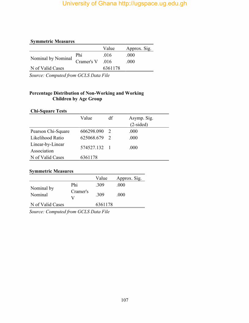
107
Symmetric Measures Value Approx. Sig.
Nominal by Nominal Phi .016 .000 Cramer's V .016 .000
N of Valid Cases 6361178 Source: Computed from GCLS Data File Percentage Distribution of Non-Working and Working
Children by Age Group Chi-Square Tests Value df Asymp. Sig.
(2-sided) Pearson Chi-Square 606298.090 2 .000 Likelihood Ratio 625068.679 2 .000 Linear-by-Linear Association
574527.132 1 .000
N of Valid Cases 6361178 Symmetric Measures Value Approx. Sig.
Nominal by Nominal
Phi .309 .000 Cramer's V .309 .000
N of Valid Cases 6361178 Source: Computed from GCLS Data File
University of Ghana http://ugspace.ug.edu.gh

108
Percentage Distribution of non-working and working Children by Size of Household
Chi-Square Tests Value df Asymp. Sig.
(2-sided) Pearson Chi-Square 86208.047 3 .000 Likelihood Ratio 86015.859 3 .000 Linear-by-Linear Association
82713.642 1 .000
N of Valid Cases 6361178 Symmetric Measures Value Approx. Sig.
Nominal by Nominal
Phi .116 .000 Cramer's V
.116 .000
N of Valid Cases 6361178 Source: Computed from GCLS Data File
Percentage Distribution of Non-Working and Working
Children by Age of Household Head
Chi-Square Tests Value df Asymp. Sig.
(2-sided) Pearson Chi-Square 94124.148 7 .000 Likelihood Ratio 95149.060 7 .000 Linear-by-Linear Association 83126.557 1 .000
N of Valid Cases 6361179
University of Ghana http://ugspace.ug.edu.gh

109
Symmetric Measures Value Approx. Sig.
Nominal by Nominal
Phi .122 .000 Cramer's V
.122 .000
N of Valid Cases 6361179 Source: Computed from GCLS Data File Percentage Distribution of Working and Non-Working Children by Literacy of Household Head Chi-Square Tests Value Df Asymp. Sig.
(2-sided) Exact Sig. (2-sided)
Exact Sig. (1-sided)
Pearson Chi-Square 188526.223 1 .000 Continuity Correction 188525.516 1 .000 Likelihood Ratio 190742.736 1 .000 Fisher's Exact Test .000 .000 Linear-by-Linear Association 188526.194 1 .000
N of Valid Cases 6361178 .
Symmetric Measures Value Approx. Sig.
Nominal by Nominal Phi .172 .000 Cramer's V .172 .000
N of Valid Cases 6361178 Source: Computed from GCLS Data File
University of Ghana http://ugspace.ug.edu.gh

110
Percentage Distribution of Working and Non-Working
Children by Level of Education of Parent
Chi-Square Tests Value df Asymp. Sig.
(2-sided) Pearson Chi-Square 329128.933 3 .000 Likelihood Ratio 325588.587 3 .000 Linear-by-Linear Association
73490.731 1 .000
N of Valid Cases 6361180 Symmetric Measures Value Approx. Sig.
Nominal by Nominal
Phi .227 .000 Cramer's V .227 .000
N of Valid Cases 6361180 Source: Computed from GCLS Data File
Percentage Distribution of Working and Non-Working Children by Parent Marital Status Chi-Square Tests Value df Asymp. Sig.
(2-sided) Exact Sig. (2-sided)
Exact Sig. (1-sided)
Pearson Chi-Square 421137.429 1 .000 Continuity Correction 421136.360 1 .000 Likelihood Ratio 421566.019 1 .000 Fisher's Exact Test .000 .000 Linear-by-Linear Association 421137.363 1 .000
N of Valid Cases 6361178
University of Ghana http://ugspace.ug.edu.gh
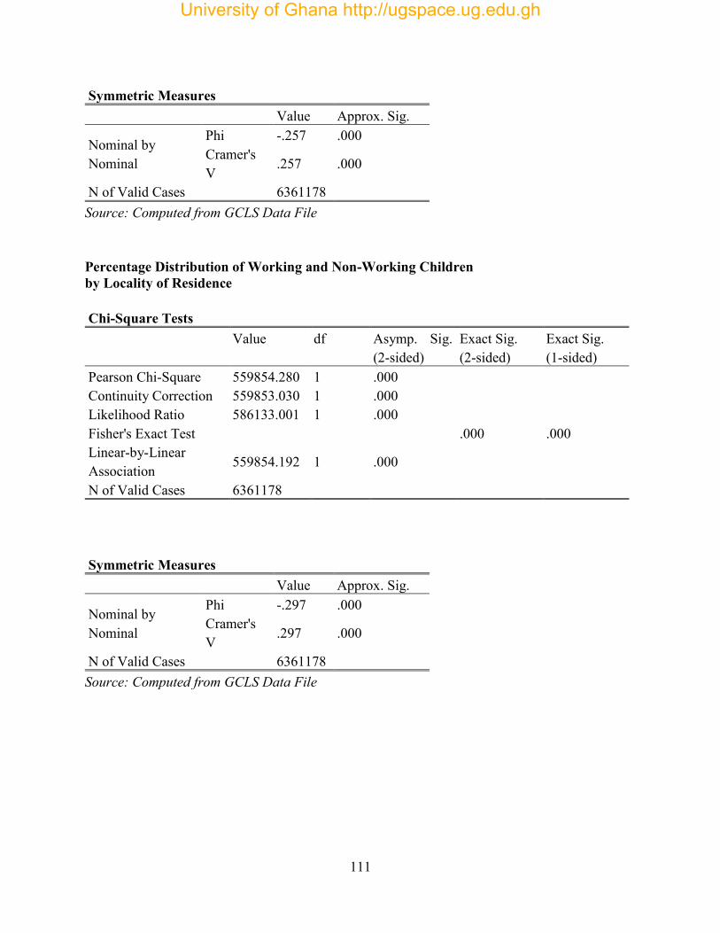
111
Symmetric Measures Value Approx. Sig.
Nominal by Nominal
Phi -.257 .000 Cramer's V
.257 .000
N of Valid Cases 6361178 Source: Computed from GCLS Data File Percentage Distribution of Working and Non-Working Children by Locality of Residence Chi-Square Tests Value df Asymp. Sig.
(2-sided) Exact Sig. (2-sided)
Exact Sig. (1-sided)
Pearson Chi-Square 559854.280 1 .000 Continuity Correction 559853.030 1 .000 Likelihood Ratio 586133.001 1 .000 Fisher's Exact Test .000 .000 Linear-by-Linear Association 559854.192 1 .000
N of Valid Cases 6361178 Symmetric Measures Value Approx. Sig.
Nominal by Nominal
Phi -.297 .000 Cramer's V .297 .000
N of Valid Cases 6361178 Source: Computed from GCLS Data File
University of Ghana http://ugspace.ug.edu.gh
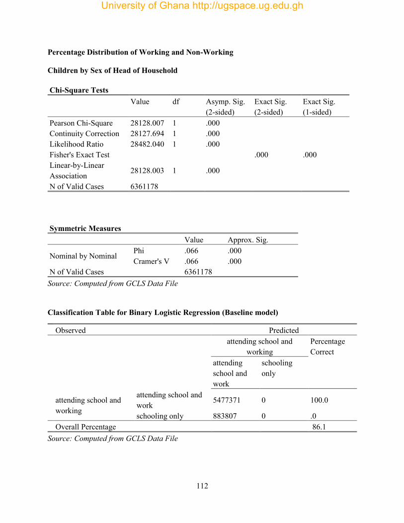
112
Percentage Distribution of Working and Non-Working
Children by Sex of Head of Household
Chi-Square Tests Value df Asymp. Sig.
(2-sided) Exact Sig. (2-sided)
Exact Sig. (1-sided)
Pearson Chi-Square 28128.007 1 .000 Continuity Correction 28127.694 1 .000 Likelihood Ratio 28482.040 1 .000 Fisher's Exact Test .000 .000 Linear-by-Linear Association
28128.003 1 .000
N of Valid Cases 6361178 Symmetric Measures Value Approx. Sig.
Nominal by Nominal Phi .066 .000 Cramer's V .066 .000
N of Valid Cases 6361178 Source: Computed from GCLS Data File Classification Table for Binary Logistic Regression (Baseline model)
Observed Predicted
attending school and
working Percentage Correct
attending school and work
schooling only
attending school and working
attending school and work 5477371 0 100.0
schooling only 883807 0 .0 Overall Percentage 86.1 Source: Computed from GCLS Data File
University of Ghana http://ugspace.ug.edu.gh

113
APPENDIX 2
Distribution of children age 5-17 years by socio-economic Variable, 2003 GCLS Socio-economic Variable Frequency Percent
Sex
Male(Ref.) 3,313,494 52.1
Female 3,047,684 47.9
Relationship to head of Household
Son/daughter (Ref.) 4,922,720 77.4
Other relations 1,438,458 22.6
Age group of children
5 - 9 (Ref.) 2,657,286 41.8
10 - 14 2,515,490 39.5
15 - 17 1,188,403 18.7
Size of Household
Less than 3 (Ref.) 105,418 1.7
3 - 4 939,200 14.8
5 - 6 2,020,048 31.8
7 - 8 1,605,209 25.2
9 - 10 1,062,152 16.7
Over 10 629,152 9.9
Residence
Urban(Ref.) 3,963,096 37.7
Rural 2,398,082 62.3
University of Ghana http://ugspace.ug.edu.gh

114
(cont‟d.)
Socio-economic Variable Frequency Percent
Age of Household Head
15 - 34 (Ref.) 682,106 10.7
35 - 39 859,832 13.5
40 - 44 978,767 15.4
45 - 49 1,007,308 15.8
50 - 54 814,128 12.8
55 - 59 495,638 7.8
60 - 64 491,379 7.7
65+ 1,032,020 16.2
Major Occupation of Parent
Farming (Ref.) 1,131,785 17.8
Service 249,813 3.9
Trade 410,596 6.5
Day/Wage Labour 188,213 3.0
Other occupation 4,380,771 68.9
Highest level of Education of Parent
No education (Ref.) 1,141,039 17.9
At most primary 4,077,352 64.1
Junior secondary 1,036,681 16.3
SSS or Higher 106,105 1.7
University of Ghana http://ugspace.ug.edu.gh

115
(cont‟d.)
Socio-economic Variable Frequency Percent
Marital status of parent
Married (Ref.) 3,757,093 59.1
Not Married 2,604,085 40.9
Region
Greater Accra (Ref.) 747,164 11.7
Western 639,438 10.1
Central 516,693 8.1
Volta 519,006 8.2
Eastern 733,780 11.5
Ashanti 988,779 15.5
Brong Ahafo 657,128 10.3
Northern 891,096 14.0
Upper East 381,988 6.0
Upper West 286,106 4.0
Literacy of household head
Not literate (Ref.) 5,610,394 88.2
Literate 750,784 11.8
Source: Computed from GCLS Data File
University of Ghana http://ugspace.ug.edu.gh
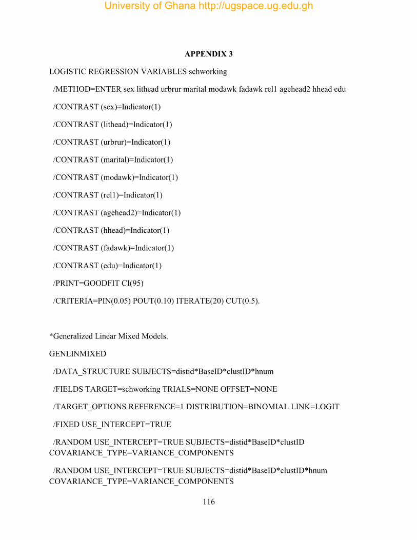
116
APPENDIX 3
LOGISTIC REGRESSION VARIABLES schworking
/METHOD=ENTER sex lithead urbrur marital modawk fadawk rel1 agehead2 hhead edu
/CONTRAST (sex)=Indicator(1)
/CONTRAST (lithead)=Indicator(1)
/CONTRAST (urbrur)=Indicator(1)
/CONTRAST (marital)=Indicator(1)
/CONTRAST (modawk)=Indicator(1)
/CONTRAST (rel1)=Indicator(1)
/CONTRAST (agehead2)=Indicator(1)
/CONTRAST (hhead)=Indicator(1)
/CONTRAST (fadawk)=Indicator(1)
/CONTRAST (edu)=Indicator(1)
/PRINT=GOODFIT CI(95)
/CRITERIA=PIN(0.05) POUT(0.10) ITERATE(20) CUT(0.5).
*Generalized Linear Mixed Models.
GENLINMIXED
/DATA_STRUCTURE SUBJECTS=distid*BaseID*clustID*hnum
/FIELDS TARGET=schworking TRIALS=NONE OFFSET=NONE
/TARGET_OPTIONS REFERENCE=1 DISTRIBUTION=BINOMIAL LINK=LOGIT
/FIXED USE_INTERCEPT=TRUE
/RANDOM USE_INTERCEPT=TRUE SUBJECTS=distid*BaseID*clustID COVARIANCE_TYPE=VARIANCE_COMPONENTS
/RANDOM USE_INTERCEPT=TRUE SUBJECTS=distid*BaseID*clustID*hnum COVARIANCE_TYPE=VARIANCE_COMPONENTS
University of Ghana http://ugspace.ug.edu.gh

117
/BUILD_OPTIONS TARGET_CATEGORY_ORDER=ASCENDING INPUTS_CATEGORY_ORDER=ASCENDING MAX_ITERATIONS=100 CONFIDENCE_LEVEL=95 DF_METHOD=RESIDUAL COVB=MODEL
/EMMEANS_OPTIONS SCALE=ORIGINAL PADJUST=SEQBONFERRONI.
*Generalized Linear Mixed Models.
GENLINMIXED
/DATA_STRUCTURE SUBJECTS=distid*BaseID*clustID*hnum
/FIELDS TARGET=schworking TRIALS=NONE OFFSET=NONE
/TARGET_OPTIONS REFERENCE=1 DISTRIBUTION=BINOMIAL LINK=LOGIT
/FIXED EFFECTS=sex agehead2 hhead marital modawk fadawk rel1 urbrur edu lithead USE_INTERCEPT=TRUE
/RANDOM USE_INTERCEPT=TRUE SUBJECTS=distid*BaseID*clustID COVARIANCE_TYPE=VARIANCE_COMPONENTS
/RANDOM USE_INTERCEPT=TRUE SUBJECTS=distid*BaseID*clustID*hnum COVARIANCE_TYPE=VARIANCE_COMPONENTS
/BUILD_OPTIONS TARGET_CATEGORY_ORDER=DESCENDING INPUTS_CATEGORY_ORDER=DESCENDING MAX_ITERATIONS=100 CONFIDENCE_LEVEL=95 DF_METHOD=RESIDUAL COVB=MODEL
/EMMEANS TABLES=sex CONTRAST=NONE
/EMMEANS TABLES=agehead2 CONTRAST=NONE
/EMMEANS TABLES=marital CONTRAST=NONE
/EMMEANS TABLES=modawk CONTRAST=NONE
/EMMEANS TABLES=fadawk CONTRAST=NONE
/EMMEANS TABLES=rel1 CONTRAST=NONE
/EMMEANS TABLES=urbrur CONTRAST=NONE
/EMMEANS TABLES=edu CONTRAST=NONE
/EMMEANS TABLES=lithead CONTRAST=NONE
University of Ghana http://ugspace.ug.edu.gh

118
/EMMEANS TABLES=hhead CONTRAST=NONE
/EMMEANS_OPTIONS SCALE=ORIGINAL PADJUST=SEQBONFERRONI.
University of Ghana http://ugspace.ug.edu.gh


