
Bank of Canada Banque du Canada
Working Paper 2005-9 / Document de travail 2005-9
State Dependence in Fundamentalsand Preferences Explains
Risk-Aversion Puzzle
by
Fousseni Chabi-Yo, René Garcia, and Eric Renault

ISSN 1192-5434
Printed in Canada on recycled paper
Bank of Canada Working Paper 2005-9
April 2005
State Dependence in Fundamentalsand Preferences Explains
Risk-Aversion Puzzle
by
Fousseni Chabi-Yo, 1 René Garcia, 2 and Eric Renault 3
1Financial Markets DepartmentBank of Canada
Ottawa, Ontario, Canada K1A [email protected]
2Département de sciences économiquesUniversité de Montréal
Montréal, Quebec, Canada H3C 3J7and CIREQ, CIRANO
3University of North Carolina at Chapel HillChapel Hill, NC 27599–3305
and CIREQ, CIRANO
The views expressed in this paper are those of the authors.No responsibility for them should be attributed to the Bank of Canada.


iii
Contents
Acknowledgements. . . . . . . . . . . . . . . . . . . . . . . . . . . . . . . . . . . . . . . . . . . . . . . . . . . . . . . . . . . . ivAbstract/Résumé. . . . . . . . . . . . . . . . . . . . . . . . . . . . . . . . . . . . . . . . . . . . . . . . . . . . . . . . . . . . . . . v
1. Introduction . . . . . . . . . . . . . . . . . . . . . . . . . . . . . . . . . . . . . . . . . . . . . . . . . . . . . . . . . . . . . . 1
2. The Pricing-Kernel and Risk-Aversion Puzzles . . . . . . . . . . . . . . . . . . . . . . . . . . . . . . . . . . 2
2.1 Theoretical underpinnings . . . . . . . . . . . . . . . . . . . . . . . . . . . . . . . . . . . . . . . . . . . . . . 2
2.2 The puzzles . . . . . . . . . . . . . . . . . . . . . . . . . . . . . . . . . . . . . . . . . . . . . . . . . . . . . . . . . . 3
2.3 Statistical methodology. . . . . . . . . . . . . . . . . . . . . . . . . . . . . . . . . . . . . . . . . . . . . . . . . 4
3. Economies with Regime Shifts . . . . . . . . . . . . . . . . . . . . . . . . . . . . . . . . . . . . . . . . . . . . . . . 5
3.1 The general framework. . . . . . . . . . . . . . . . . . . . . . . . . . . . . . . . . . . . . . . . . . . . . . . . . 6
3.2 State-dependent preferences or fundamentals . . . . . . . . . . . . . . . . . . . . . . . . . . . . . . . 8
3.3 Simulating options and stock prices . . . . . . . . . . . . . . . . . . . . . . . . . . . . . . . . . . . . . . 10
4. Empirical Results . . . . . . . . . . . . . . . . . . . . . . . . . . . . . . . . . . . . . . . . . . . . . . . . . . . . . . . . . 11
4.1 Choosing preference and fundamental parameters . . . . . . . . . . . . . . . . . . . . . . . . . . . 11
4.2 Regime shifts in fundamentals . . . . . . . . . . . . . . . . . . . . . . . . . . . . . . . . . . . . . . . . . . 12
4.3 Regime shifts in preferences. . . . . . . . . . . . . . . . . . . . . . . . . . . . . . . . . . . . . . . . . . . . 13
4.4 General comments . . . . . . . . . . . . . . . . . . . . . . . . . . . . . . . . . . . . . . . . . . . . . . . . . . . 13
5. Conclusion . . . . . . . . . . . . . . . . . . . . . . . . . . . . . . . . . . . . . . . . . . . . . . . . . . . . . . . . . . . . . . 14
References. . . . . . . . . . . . . . . . . . . . . . . . . . . . . . . . . . . . . . . . . . . . . . . . . . . . . . . . . . . . . . . . . . . 15
Figures. . . . . . . . . . . . . . . . . . . . . . . . . . . . . . . . . . . . . . . . . . . . . . . . . . . . . . . . . . . . . . . . . . . . . . 17
Appendix. . . . . . . . . . . . . . . . . . . . . . . . . . . . . . . . . . . . . . . . . . . . . . . . . . . . . . . . . . . . . . . . . . . . 23

iv
Acknowledgements
The authors gratefully acknowledge financial support from the Fonds québécois de recherche sur
la société et la culture (FQRSC), the Social Sciences and Humanities Research Council of Canada
(SSHRC), the Mathematics of Information Technology and Complex Systems (MITACS), a
Network of Centres of Excellence. The second author is grateful to Hydro-Québec and the Bank
of Canada Fellowship for financial support.

v
Abstract
The authors examine the ability of economic models with regime shifts to rationalize and explain
the risk-aversion and pricing-kernel puzzles put forward in Jackwerth (2000). They build an
economy where investors’ preferences or economic fundamentals are state-dependent, and
simulate prices for a market index and European options on that index. Based on the original non-
parametric methodology, the risk-aversion and pricing-kernel functions obtained across wealth
states with these artificial data exhibit the same puzzles found with the actual data, but within each
regime the puzzles disappear. This suggests that state dependence potentially explains the puzzles.
JEL classification: G12, G13Bank classification: Financial markets; Market structure and pricing
Résumé
Les auteurs présentent un modèle économique à changement de régime qui permet de reproduire
les énigmes relatives à l’aversion pour le risque et au facteur d’actualisation stochastique mises en
évidence par Jackwerth (2000). Ils construisent un modèle où les préférences des investisseurs et
leur consommation dépendent d’une variable d’état qui suit un processus de type markovien à
deux régimes et génèrent une série de prix d’options d’achat européennes. Au moyen de la
méthodologie d’estimation non paramétrique proposée par Jackwerth, ils déduisent des fonctions
d’aversion absolue pour le risque et d’actualisation stochastique pour chaque valeur de la richesse.
Ces fonctions présentent les mêmes anomalies que celles obtenues par Jackwerth à partir des
données réelles. Lorsque la même méthodologie est appliquée à chaque état de l’économie, les
anomalies disparaissent. D’après ces résultats, l’existence de changements de régime dans
l’économie pourrait expliquer ces deux énigmes.
Classification JEL : G12, G13Classification de la Banque : Marchés financiers; Structure de marché et fixation des prix


1. Introduction
Recently, Jackwerth (2000) and Aït-Sahalia and Lo (2000) have proposed non-parametric
approaches to recover risk-aversion functions across wealth states from observed stock and options
prices. In a complete market economy, which implies the existence of a representative investor,
absolute risk aversion (ARA) can be evaluated for any state of wealth in terms of the historical and
risk-neutral distributions. To obtain the historical distribution, Jackwerth (2000) applied a non-
parametric kernel density approach to a time series of returns on the Standard & Poor’s (S&P) 500
index. The risk-neutral distribution is recovered from prices on European call options written on
the S&P 500 index by applying a variation of the non-parametric method introduced in Jackwerth
and Rubinstein (1996). The basic idea of this method is to search for the smoothest risk-neutral
distribution, which at the same time explains the options prices.
Using options prices and realized returns, Jackwerth (2000) and Jackwerth and Rubinstein
(2004) find estimated values for the ARA that are nearly consistent with economic theory before
the 1987 crash. However, for the post-crash period, Jackwerth (2000) finds that the implied ARA
function is negative around the mean and increasing for larger wealth levels. This empirical feature,
called the risk-aversion puzzle by Jackwerth (2000), has also been documented by Aït-Sahalia and
Lo (2000). Another way to express this puzzling result is through the pricing kernel across wealth
states. A pricing-kernel puzzle occurs when the ratio of the state-price density to the historical
density increases with wealth (see Brown and Jackwerth 2000). After examining several potential
explanations, Jackwerth (2000) concludes that these puzzling results are most probably due to the
mispricing of some options by the market.
In this paper, we propose another explanation based on the existence of state dependence in
preferences or in economic fundamentals. Garcia, Luger, and Renault (2001) propose a general
pricing model where the pricing kernel depends on some latent state variables, observed only
by the investor. This phenomenon can be understood in either of two possible ways: (i) as in
Melino and Yang (2003), investors’ preferences are state-dependent; or, (ii) as in Garcia, Luger,
and Renault (2003), the joint process of consumption and dividends follows a Markov-switching
regime distribution such that the current regime is known only to the investors. In this paper,
we use the models developed in Garcia, Luger, and Renault (2003) and Melino and Yang (2003)
to generate artificial prices for stocks and options. To recover the risk-neutral distribution, we
develop a simple simulation method to create a bid-ask spread around options prices and apply the
same non-parametric methodology as Jackwerth and Rubinstein (1996). The historical distribution
is estimated based on a mixture of lognormals. In our model, by construction, the risk-aversion
functions are consistent with economic theory within each regime, since the regime is observed
1

by investors. As in Jackwerth (2000), however, we obtain negative estimates of the risk-aversion
function in some states of wealth. The pricing-kernel function across wealth states also exhibits a
puzzle, even though this function is decreasing within each regime. We therefore provide another
potential explanation for the puzzles put forward by Jackwerth (2000).
The remainder of this paper is organized as follows. In section 2, we present Jackwerth’s (2000)
approach for recovering the ARA function across wealth states. In section 3, we build a utility-
based economic model with state dependence in preferences and endowments, and describe how
to simulate artificial options and stock prices in this economy. In section 4, we recover the risk-
aversion and pricing-kernel functions across wealth states and discuss the results. In section 5, we
offer some conclusions.
2. The Pricing-Kernel and Risk-Aversion Puzzles
In this section, we outline the puzzles put forward by Jackwerth (2000) as well as the method-
ology used to exhibit those puzzles.
2.1 Theoretical underpinnings
Under very general non-arbitrage conditions (Hansen and Richard 1987), the time t price of
an asset that delivers a payoff gt+1 at time (t+ 1) is given by:
pt = Et [mt+1gt+1] , (1)
where Et [.] denotes the conditional expectation operator given investors’ information at time t.
Any random variable mt+1 consistent with (1) is called an admissible stochastic discount factor
(SDF), or pricing kernel. Among the admissible SDFs, only one, denoted by m∗t+1, is a function
of available payoffs. It is the orthogonal projection of any admissible SDF on the set of payoffs.
Suppose some rational investor is able to separate its utility over current and future values of
consumption:
U [Ct, Ct+1] = u(Ct) + βu (Ct+1) . (2)
The first-order condition for an optimal consumption and portfolio choice will imply that m∗t+1coincides with the projection of β u (Ct+1)u (Ct)
on the set of payoffs. Therefore, through a convenient
aggregation argument, the concavity of utility functions should imply that m∗t+1 is decreasing in
current wealth.
Moreover, as Hansen and Richard (1987) show, no arbitrage implies almost sure positivity
of m∗t+1. Therefore, m∗t+1/Etm∗t+1 can be interpreted as the density function of the risk-neutral
2
probability distribution with respect to the historical one. In the case of a representative investor
with preferences consistent with (2), we deduce:
m∗t+1Etm∗t+1
=u (Ct+1)
Etu (Ct+1).
Therefore,∂Logm∗t+1∂Ct+1
=u (Ct+1)
u (Ct+1)(3)
is the inverse of the Arrow-Pratt index of the ARA of the investor.
2.2 The puzzles
For the sake of simplicity, it is convenient to analyze these puzzles in a finite state-space
framework. If j = 1, · · · , n denotes the possible states of nature, we get the density function of therisk-neutral distribution probability with respect to the historical one as:
m∗t+1Etm∗t+1
=p∗jpjin state j, (4)
where p∗j is the risk-neutral probability across wealth states j = 1, · · · , n and pj is the correspondinghistorical probability. Brown and Jackwerth (2000) use (4) to empirically derive the pricing-kernel
function from realized returns on the S&P 500 index and options prices on the index over a post-
1987 period. For the centre wealth states (over the range of 0.97 to 1.03, with average wealth
normalized to one), they find a pricing-kernel function that is increasing in wealth. This is the
so-called pricing-kernel puzzle.
As explained in section 2.1, the increasing nature of function (1) in wealth is puzzling because it
is akin to a convex utility function for a representative investor, which is obviously inconsistent with
the general assumption of risk aversion. From (3), the ARA coefficient can actually be computed
through a log-derivative of the pricing kernel. By using (4), we deduce:
ARA = −u (Ct+1)
u (Ct+1)=pjpj− p
∗j
p∗j, (5)
where pj and p∗j are the derivatives of pj and p
∗j with respect to aggregate wealth in state j.
Jackwerth (2000) observes that the ARA functions computed from (5) dramatically change
shape around the 1987 crash. Prior to the crash, they are positive and decreasing in wealth, which
is consistent with standard assumptions made in economic theory about investors’ preferences.
After the crash, they are partially negative and increasing (see Figure 3 in Jackwerth 2000). This
result is called the risk-aversion puzzle. One component of it is equivalent to the pricing-kernel
puzzle: ARA should be positive, because the pricing kernel should be decreasing in aggregate
3
wealth. Additionally, even when there is no pricing-kernel puzzle (positive ARA), there remains a
risk-aversion puzzle when ARA is increasing in wealth. While the pricing-kernel puzzle is observed
for only (the centre) wealth states, the risk-aversion puzzle (increasing ARA) remains for larger
levels of wealth. Without any discretization of wealth states, Aït-Sahalia and Lo (2000) document
similar empirical puzzles for implied risk aversion.
2.3 Statistical methodology
It is possible to use several statistical methodologies to recover the historical distribution of
future returns (on the underlying index), given current returns. As Jackwerth (2000) emphasizes,
the choice of a particular estimation strategy should not have any impact on the documented
puzzles. For instance, a kernel estimation will be valid under very general stationarity and mixing
conditions.
While historical probabilities, pj, are recovered from a time series of underlying index returns,
risk-neutral probabilities, p∗j , will be backed out of cross-sections from a set of observed options
prices written on the same index. Concerning the latter, in a pioneering article, Jackwerth and
Rubinstein (1996) recommend solving the following quadratic program:
minp∗
n
j=1
p∗j − p̄j 2
n
j=1
p∗j = 1, p∗j ≥ 0,
C∗i =1
Rf
n
j=1
p∗j max [0, Sj −Ki] , (6)
1
Rf
n
j=1
p∗jSj = S0,
C∗ib ≤ C∗i ≤ C∗ia for i = 1,...,m and Sb ≤ S0 ≤ Sa,
where C∗ib (C∗ia) represents the call options bid (ask) price with strike price Ki. The bid and ask
stock prices are, respectively, Sb and Sa. In other words, the implied risk-neutral probabilities, p∗j ,
are the closest to the prior ones, p̄j , that result in options and underlying asset values that fall
between the respective bid and ask prices. As Jackwerth and Rubinstein (1996) emphasize, this
methodology has the virtue that general arbitrage opportunities do not exist if and only if there
is a solution. This remark is still valid when considering alternative quadratic programs based on
4
other distances. For instance, Jackwerth and Rubinstein (1996) put forward the goodness-of-fit
approach:
minp∗
n
j=1
p∗j − p̄j2
p̄j, (7)
whereas, following Hansen and Jagannathan (1997), one may prefer:
minp∗
n
j=1
p∗j − p̄j2
pj, (8)
since, with obvious notations, the objective function (8) can be seen as Et(m∗t+1 −mt+1)2.Jackwerth and Rubinstein (1996), however, observe that the implied distributions are rather
independent of the choice of the objective function when a sufficiently high number of options are
available.1
Since we wish to focus on a simulation exercise, we will choose 50 options in cross-section to
be sure that the solution is determined by the constraints (options and underlying asset values
between bid and ask prices), and not by the objective function. In particular, the choice of the
prior is immaterial and, as Jackwerth and Rubinstein (1996) note, even a pure smoothness criterion
independent of any prior would do the job. They consider, in particular:
minp∗
n
j=1
p∗j−1 + p∗j+1 − 2p∗j 2
, (9)
when the states j = 1, 2 · · · , n are ranked in order of increasing wealth. To remain true to thetraditional approach, however, in section 4 we will use the goodness-of-fit criterion in the simulation.
Prior risk-neutral probabilities, p̄j , will be computed, according to Breeden and Litzenberger’s
(1978) methodology, from second-order derivatives of options prices with respect to the strike
price. Note that a necessary source of difference between p∗j and p̄j is the discretization of the
state-space performed to define p∗j .
3. Economies with Regime Shifts
In this section, we construct economies with regime shifts in endowments or preferences to
simulate artificial stock and options prices.
1They notice that “as few as 8 option prices seem to contain enough information to determine the general shape
of the implied distribution” and that “at the extreme, the constraints themselves will completely determine the
solution.”
5
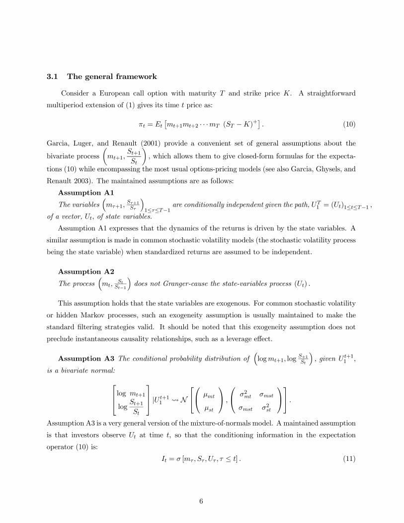
3.1 The general framework
Consider a European call option with maturity T and strike price K. A straightforward
multiperiod extension of (1) gives its time t price as:
πt = Et mt+1mt+2 · · ·mT (ST −K)+ . (10)
Garcia, Luger, and Renault (2001) provide a convenient set of general assumptions about the
bivariate process mt+1,St+1St
, which allows them to give closed-form formulas for the expecta-
tions (10) while encompassing the most usual options-pricing models (see also Garcia, Ghysels, and
Renault 2003). The maintained assumptions are as follows:
Assumption A1
The variables mτ+1,Sτ+1Sτ 1≤τ≤T−1
are conditionally independent given the path, UT1 = (Ut)1≤t≤T−1 ,
of a vector, Ut, of state variables.
Assumption A1 expresses that the dynamics of the returns is driven by the state variables. A
similar assumption is made in common stochastic volatility models (the stochastic volatility process
being the state variable) when standardized returns are assumed to be independent.
Assumption A2
The process mt,StSt−1 does not Granger-cause the state-variables process (Ut) .
This assumption holds that the state variables are exogenous. For common stochastic volatility
or hidden Markov processes, such an exogeneity assumption is usually maintained to make the
standard filtering strategies valid. It should be noted that this exogeneity assumption does not
preclude instantaneous causality relationships, such as a leverage effect.
Assumption A3 The conditional probability distribution of logmt+1, logS+1St
, given U t+11 ,
is a bivariate normal: log mt+1log
St+1St
|U t+11 N µmt
µst
, σ2mt σmst
σmst σ2st
.Assumption A3 is a very general version of the mixture-of-normals model. A maintained assumption
is that investors observe Ut at time t, so that the conditioning information in the expectation
operator (10) is:
It = σ [mτ , Sτ , Uτ , τ ≤ t] . (11)
6

In our simulation exercise, the mixing variable, Ut+1, will be a two-state Markov chain with a
transition matrix:
P =
p00 1− p001− p11 p11
. (12)
Indeed, following Garcia, Luger, and Renault (2001), a general options-pricing formula can be
stated for any Markov process (Ut) conformable to A1, A2, and A3.
Proposition 3.1 Under assumptions A1, A2, and A3,
πtSt= πt(xt) = Et Qms (t, T )Φ (d1(xt))− B̃ (t, T )
B (t, T )e−xtΦ (d2 (xt)) ,
where xt = log StKB(t,T ) , B (t, T ) = Et
T−1
τ=t
mτ+1 is the time t price of a bond maturing at time
T, and
d1 (x) =x
σ̄t,T+
σ̄t,T2+
1
σ̄t,Tlog Qms (t, T )
B (t, T )
B̃ (t, T ),
d2 (x) = d1 (x)− σ̄t,T ,
σ̄2t,T =T−1
τ=t
σ2sτ ,
and
B̃ (t, T ) = expT−1
τ=t
µmτ+1 +1
2
T−1
τ=t
σ2mτ , ,
Qms (t, T ) = B̃ (t, T ) expT−1
τ=t
σmsτ+1 ESTSt|UT1 .
As explicitly analyzed in Garcia, Ghysels, and Renault (2003), this general options-pricing
formula encompasses most of the common pricing formulas for European options on equity.
To consider economically meaningful regime shifts in the SDF, it is convenient to start from a
two-factor model as produced by Epstein and Zin (1989). Their recursive utility framework leads
them to the following SDF:
mt+1 = βCt+1Ct
−ρ γ1
Rmt+1
1−γ, (13)
where ρ = 1− 1σ, σ is the elasticity of intertemporal substitution and γ =
α
ρwith (1− α) the index
of relative risk aversion. With a two-state mixing variable, Ut+1, logmt+1 appears as a mixture of
7
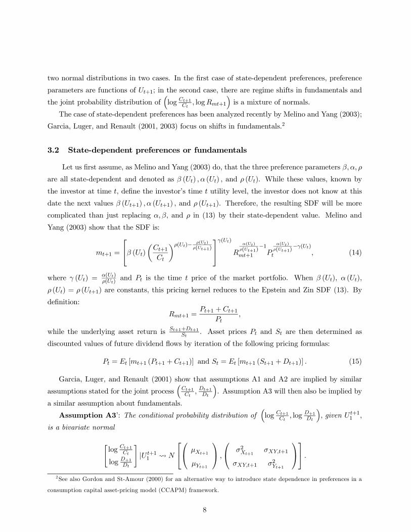
two normal distributions in two cases. In the first case of state-dependent preferences, preference
parameters are functions of Ut+1; in the second case, there are regime shifts in fundamentals and
the joint probability distribution of log Ct+1Ct, logRmt+1 is a mixture of normals.
The case of state-dependent preferences has been analyzed recently by Melino and Yang (2003);
Garcia, Luger, and Renault (2001, 2003) focus on shifts in fundamentals.2
3.2 State-dependent preferences or fundamentals
Let us first assume, as Melino and Yang (2003) do, that the three preference parameters β,α, ρ
are all state-dependent and denoted as β (Ut) ,α (Ut) , and ρ (Ut). While these values, known by
the investor at time t, define the investor’s time t utility level, the investor does not know at this
date the next values β (Ut+1) ,α (Ut+1) , and ρ (Ut+1). Therefore, the resulting SDF will be more
complicated than just replacing α,β, and ρ in (13) by their state-dependent value. Melino and
Yang (2003) show that the SDF is:
mt+1 =
β (Ut) Ct+1Ct
ρ(Ut)− ρ(Ut)
ρ(Ut+1)
γ(Ut)R α(Ut)
ρ(Ut+1)−1
mt+1 P
α(Ut)
ρ(Ut+1)−γ(Ut)
t , (14)
where γ (Ut) =α(Ut)ρ(Ut)
and Pt is the time t price of the market portfolio. When β (Ut), α (Ut),
ρ (Ut) = ρ (Ut+1) are constants, this pricing kernel reduces to the Epstein and Zin SDF (13). By
definition:
Rmt+1 =Pt+1 +Ct+1
Pt,
while the underlying asset return is St+1+Dt+1St
. Asset prices Pt and St are then determined as
discounted values of future dividend flows by iteration of the following pricing formulas:
Pt = Et [mt+1 (Pt+1 +Ct+1)] and St = Et [mt+1 (St+1 +Dt+1)] . (15)
Garcia, Luger, and Renault (2001) show that assumptions A1 and A2 are implied by similar
assumptions stated for the joint process Ct+1Ct, Dt+1Dt
. Assumption A3 will then also be implied by
a similar assumption about fundamentals.
Assumption A3’: The conditional probability distribution of log Ct+1Ct, log D+1Dt
, given U t+11 ,
is a bivariate normal
log Ct+1Ct
log D+1Dt
|U t+11 N
µXt+1
µYt+1
, σ2Xt+1 σXY,t+1
σXY,t+1 σ2Yt+1
.2See also Gordon and St-Amour (2000) for an alternative way to introduce state dependence in preferences in a
consumption capital asset-pricing model (CCAPM) framework.
8
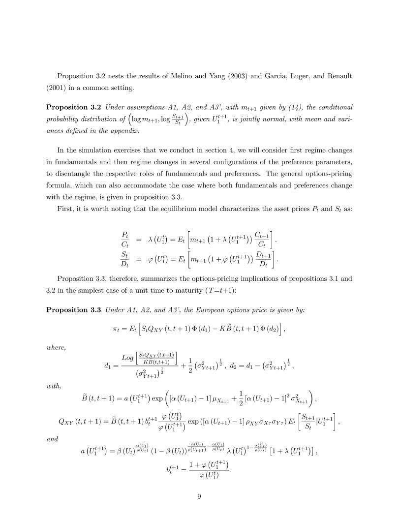
Proposition 3.2 nests the results of Melino and Yang (2003) and Garcia, Luger, and Renault
(2001) in a common setting.
Proposition 3.2 Under assumptions A1, A2, and A3’, with mt+1 given by (14), the conditional
probability distribution of logmt+1, logSt+1St
, given U t+11 , is jointly normal, with mean and vari-
ances defined in the appendix.
In the simulation exercises that we conduct in section 4, we will consider first regime changes
in fundamentals and then regime changes in several configurations of the preference parameters,
to disentangle the respective roles of fundamentals and preferences. The general options-pricing
formula, which can also accommodate the case where both fundamentals and preferences change
with the regime, is given in proposition 3.3.
First, it is worth noting that the equilibrium model characterizes the asset prices Pt and St as:
PtCt
= λ U t1 = Et mt+1 1 + λ U t+11
Ct+1Ct
.
StDt
= ϕ U t1 = Et mt+1 1 + ϕ U t+11
Dt+1Dt
.
Proposition 3.3, therefore, summarizes the options-pricing implications of propositions 3.1 and
3.2 in the simplest case of a unit time to maturity (T=t+1):
Proposition 3.3 Under A1, A2, and A3’, the European options price is given by:
πt = Et StQXY (t, t+ 1)Φ (d1)−KB (t, t+ 1)Φ (d2) ,
where,
d1 =Log StQXY (t,t+1)
KB(t,t+1)
σ2Y t+112
+1
2σ2Y t+1
12 , d2 = d1 − σ2Y t+1
12 ,
with,
B (t, t+ 1) = a U t+11 exp [α (Ut+1)− 1]µXt+1 +1
2[α (Ut+1)− 1]2 σ2Xt+1 ,
QXY (t, t+ 1) = B (t, t+ 1) bt+1t
ϕ U t1ϕ U t+11
exp ([α (Ut+1)− 1] ρXY σXτσY τ )EtSt+1St
|U t+11 ,
and
a U t+11 = β (Ut)α(Ut)ρ(Ut) (1− β (Ut))
α(Ut)
ρ(Ut+1)−α(Ut)
ρ(Ut) λ U t11−α(Ut)
ρ(Ut) 1 + λ U t+11 ,
bt+1t =1 + ϕ U t+11
ϕ (U t1).
9

P . The proof is similar to the proof where α (Ut) , β (Ut) , and ρ (Ut) are constants, which is
given in Garcia, Luger, and Renault (2003).
If the preference parameters α, β, and ρ are constants, proposition 3.3 collapses to the Gar-
cia, Luger, and Renault (2001) options-pricing formula. Note that the definition of λ U t+11 and
ϕ U t+11 is equivalent to: EtQXY (t, t+ 1) = 1, and EtB (t, t+ 1) = B (t, t+ 1) .
3.3 Simulating options and stock prices
First, we calibrate our economic models with regime shifts in the parameters describing pref-
erences or economic fundamentals.3 We then use proposition 3.3 to compute options prices with
different strike prices. To use the methodology described in (7), we need to develop a simple
technique to create bid-ask spreads around the simulated prices. This is done in three steps:
• Step 1: Given the stock price, St, we find a bid-ask spread, sp, by drawing in a lognormaldistribution:
log (sp)→ N µsp,σ2sp ,
where the parameters µsp and σ2sp are chosen exogenously.
• Step 2: Given sp, we draw a real number, x, in the censored normal probability distributionN(µx,σ
2x), given 0 ≤ x ≤ sp.
• Step 3: We then compute the stock bid and ask prices:
ask price = St + (sp− ex) ,bid price = St − ex.
We apply a similar simulation methodology to create bid and ask prices for options. Based on
these bid and ask options prices and stock prices, we recover the risk-neutral probabilities using
the non-parametric methodology described in section 2. It is important to note that our Monte
Carlo approach gives us the historical return distribution. Therefore, we do not need to use any
non-parametric estimation technique to recover the historical distribution.
The whole procedure must be applied for each state Ut ∈ {0, 1} of the economy. At date t,given the state variable value, Ut ∈ {0, 1} , we compute the call option prices:
πt (Ut) = E StQXY (t, t+ 1)Φ (d1)−KB (t, t+ 1)Φ (d2) |Ut ,3 In the case of state-dependent fundamentals, we choose values that are close to those estimated in Garcia, Luger,
and Renault (2003), where preference parameters are not state-dependent. For state-dependent preferences, we
disturb these particular values. All values used are explicitly given in Figures 1 to 6.
10

and perform steps 1, 2, and 3. We then use equations (4) and (5) to infer the conditional ARA and
pricing-kernel functions across states (given the state variable, Ut).
By construction, these quantities are computed from probabilities pj (Ut) and p∗j (Ut) , which
explicitly depend on the actual value of the latent state, Ut. By contrast, a statistician who does not
observe the state and performs a non-parametric estimation of the stationary historical distribution
that does not account for unobserved heterogeneity, will estimate marginal probabilities, pj, that
are averaged across states:
pj = P (Ut = 0) pj (0) + P (Ut = 1) pj (1) . (16)
As far as risk-neutral probability, p∗j , is concerned, the issue is less clear. If we could be sure
that not only the agents have observed the state Ut but also that the statistical observation of asset
prices is synchronized with observations, then the p∗j computed from (6) and the real data should
be p∗j (Ut). Any synchronization problem, however, may push the implied p∗j towards their averaged
values:
p∗j = P (Ut = 0) p∗j (0) + P (Ut = 1) p
∗j (1) . (17)
For reasons made explicit below, we choose to compare the implied risk aversion and pricing
kernel computed state-by-state from pj (Ut) , p∗j (Ut) with the fully marginalized ones; that is,
computed from marginalized values pj, p∗j given by (16) and (17), rather than using the possible
mixed approach pj, p∗j (Ut) .
4. Empirical Results
4.1 Choosing preference and fundamental parameters
In the case of state-dependent fundamentals, we choose values that are close to those estimated
in Garcia, Luger, and Renault (2003), where preference parameters are not state-dependent. Garcia,
Luger, and Renault propose a utility-based options-pricing model with stochastic volatility and
jumps features. Their model is cast within the recursive utility framework of Epstein and Zin (1989),
in which the roles of discounting risk aversion and intertemporal substitution are disentangled.
Garcia, Luger, and Renault use daily price data for S&P 500 index European call options obtained
from the Chicago Board Options Exchange for the period January 1991 to December 1995. They
also use daily return data for the S&P 500 index and estimate preferences parameters in S&P
500 options prices. They find quite reasonable values for the coefficient of the risk aversion and
the intertemporal elasticity of substitution. Depending on the sample period used, estimates are
in the range of (-8.75,-4) (see Table 5 in their paper). Garcia, Luger, and Renault’s estimation
11
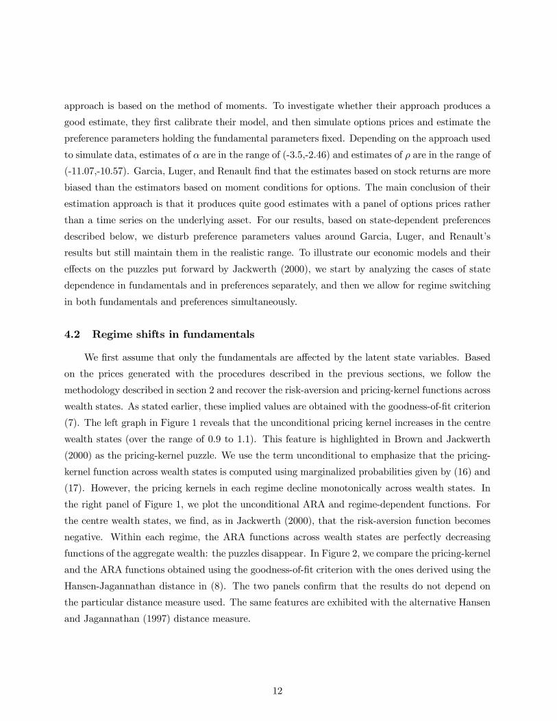
approach is based on the method of moments. To investigate whether their approach produces a
good estimate, they first calibrate their model, and then simulate options prices and estimate the
preference parameters holding the fundamental parameters fixed. Depending on the approach used
to simulate data, estimates of α are in the range of (-3.5,-2.46) and estimates of ρ are in the range of
(-11.07,-10.57). Garcia, Luger, and Renault find that the estimates based on stock returns are more
biased than the estimators based on moment conditions for options. The main conclusion of their
estimation approach is that it produces quite good estimates with a panel of options prices rather
than a time series on the underlying asset. For our results, based on state-dependent preferences
described below, we disturb preference parameters values around Garcia, Luger, and Renault’s
results but still maintain them in the realistic range. To illustrate our economic models and their
effects on the puzzles put forward by Jackwerth (2000), we start by analyzing the cases of state
dependence in fundamentals and in preferences separately, and then we allow for regime switching
in both fundamentals and preferences simultaneously.
4.2 Regime shifts in fundamentals
We first assume that only the fundamentals are affected by the latent state variables. Based
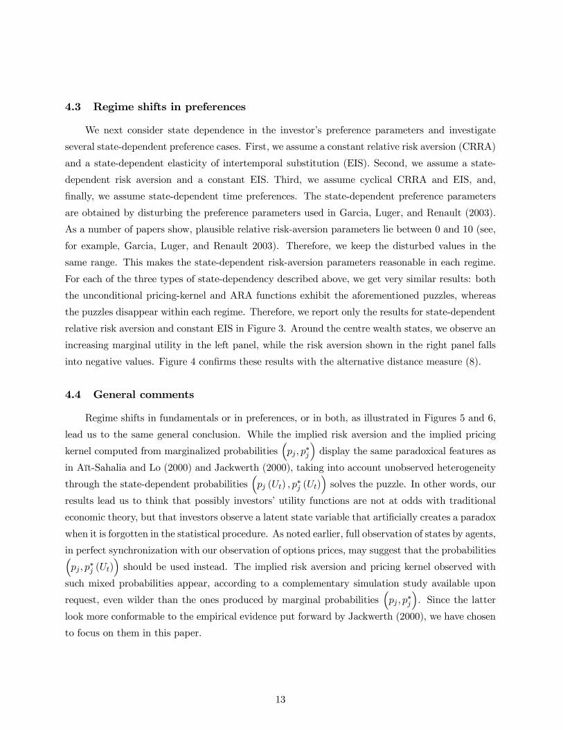
on the prices generated with the procedures described in the previous sections, we follow the
methodology described in section 2 and recover the risk-aversion and pricing-kernel functions across
wealth states. As stated earlier, these implied values are obtained with the goodness-of-fit criterion
(7). The left graph in Figure 1 reveals that the unconditional pricing kernel increases in the centre
wealth states (over the range of 0.9 to 1.1). This feature is highlighted in Brown and Jackwerth
(2000) as the pricing-kernel puzzle. We use the term unconditional to emphasize that the pricing-
kernel function across wealth states is computed using marginalized probabilities given by (16) and
(17). However, the pricing kernels in each regime decline monotonically across wealth states. In
the right panel of Figure 1, we plot the unconditional ARA and regime-dependent functions. For
the centre wealth states, we find, as in Jackwerth (2000), that the risk-aversion function becomes
negative. Within each regime, the ARA functions across wealth states are perfectly decreasing
functions of the aggregate wealth: the puzzles disappear. In Figure 2, we compare the pricing-kernel
and the ARA functions obtained using the goodness-of-fit criterion with the ones derived using the
Hansen-Jagannathan distance in (8). The two panels confirm that the results do not depend on
the particular distance measure used. The same features are exhibited with the alternative Hansen
and Jagannathan (1997) distance measure.
12
4.3 Regime shifts in preferences
We next consider state dependence in the investor’s preference parameters and investigate
several state-dependent preference cases. First, we assume a constant relative risk aversion (CRRA)
and a state-dependent elasticity of intertemporal substitution (EIS). Second, we assume a state-
dependent risk aversion and a constant EIS. Third, we assume cyclical CRRA and EIS, and,
finally, we assume state-dependent time preferences. The state-dependent preference parameters
are obtained by disturbing the preference parameters used in Garcia, Luger, and Renault (2003).
As a number of papers show, plausible relative risk-aversion parameters lie between 0 and 10 (see,
for example, Garcia, Luger, and Renault 2003). Therefore, we keep the disturbed values in the
same range. This makes the state-dependent risk-aversion parameters reasonable in each regime.
For each of the three types of state-dependency described above, we get very similar results: both
the unconditional pricing-kernel and ARA functions exhibit the aforementioned puzzles, whereas
the puzzles disappear within each regime. Therefore, we report only the results for state-dependent
relative risk aversion and constant EIS in Figure 3. Around the centre wealth states, we observe an
increasing marginal utility in the left panel, while the risk aversion shown in the right panel falls
into negative values. Figure 4 confirms these results with the alternative distance measure (8).
4.4 General comments
Regime shifts in fundamentals or in preferences, or in both, as illustrated in Figures 5 and 6,
lead us to the same general conclusion. While the implied risk aversion and the implied pricing
kernel computed from marginalized probabilities pj, p∗j display the same paradoxical features as
in Aït-Sahalia and Lo (2000) and Jackwerth (2000), taking into account unobserved heterogeneity
through the state-dependent probabilities pj (Ut) , p∗j (Ut) solves the puzzle. In other words, our
results lead us to think that possibly investors’ utility functions are not at odds with traditional
economic theory, but that investors observe a latent state variable that artificially creates a paradox
when it is forgotten in the statistical procedure. As noted earlier, full observation of states by agents,
in perfect synchronization with our observation of options prices, may suggest that the probabilities
pj , p∗j (Ut) should be used instead. The implied risk aversion and pricing kernel observed with
such mixed probabilities appear, according to a complementary simulation study available upon
request, even wilder than the ones produced by marginal probabilities pj , p∗j . Since the latter
look more conformable to the empirical evidence put forward by Jackwerth (2000), we have chosen
to focus on them in this paper.
13

5. Conclusion
In this paper, we have investigated the ability of economic models with regime shifts to pro-
duce and solve the risk-aversion and the pricing-kernel puzzles put forward by Aït-Sahalia and Lo
(2000) and Jackwerth (2000). We have shown that models with regime shifts in fundamentals or
an investor’s preferences can explain and rationalize these puzzles. The ARA and pricing-kernel
functions extracted from the simulated prices in these economies exhibit the same puzzling features
as in papers by previous researchers, and are inconsistent with the usual assumptions of decreasing
marginal utility and positive risk aversion. Within each regime, however, the ARA and pricing-
kernel functions are consistent with economic theory: the investor’s utility is concave and their
risk aversion remains positive. In other words, investor behaviour is not at odds with economic
theory, but depends on some factors that the statistician does not observe. We have shown that
this conclusion is robust to the choice of the statistical estimation procedure.
14

References
Aït -S ah alia , Y. a nd A.W. L o. 200 0. “No np ar amet ric R is k Ma na geme nt an d I m pl ied R is k
Aversion.” Journal of Econometrics 94(1-2): 9—51.
Breeden, D. and R. Litzenberger. 1978. “Prices of State-Contingent Claims Implicit in Option
Prices.” Journal of Business 51(4): 621—51.
Brown, P. and J.C. Jackwerth. 2000. “The Pricing Kernel Puzzle: Reconciling Index Option
Data and Economic Theory.” University of Wisconsin at Madison, Finance Department, School
of Business Working Paper.
Epstein, L. and S. Zin. 1989. “Substitution, Risk Aversion, and the Temporal Behavior of
Consumption and Asset Returns: A Theoretical Framework.” Econometrica 57(4): 937—69.
Garcia, R., E. Ghysels, and E. Renault. 2003. “The Econometrics of Option Pricing.” In
Handbook of Financial Econometrics, edited by Y. Aït-Sahalia and L.P. Hansen. Amsterdam:
Elsevier/ North Holland.
Garcia, R., R. Luger, and E. Renault. 2001. “Asymmetric Smiles, Leverage Effects and Struc-
tural Parameters.” Cirano Working Paper No. 2001s-01.
–—. 2003. “Empirical Assessment of an Intertemporal Option Pricing Model with Latent
Variables.” Journal of Econometrics 116(1-2): 49—83.
Gordon, S. and P. St-Amour. 2000. “A Preference Regime Model of Bull and Bear Markets.”
American Economic Review 90(4): 1019—33.
Hansen, L. and R. Jagannathan. 1997. “Assessing Specification Errors in Stochastic Discount
Factor Models.” Journal of Finance 52(2): 557—90.
Hansen, L. and S. Richard. 1987. “The Role of Conditioning Information in Deducing Testable
Restrictions Implied by Dynamic Asset Pricing Models.” Econometrica 55(3): 587—613.
Jackwerth, J.C. 2000. “Recovering Risk Aversion from Option Prices and Realized Returns.”
Review of Financial Studies 13(2): 433—51.
Jackwerth, J.C. and M. Rubinstein. 1996. “Recovering Probability Distributions from Option
Prices.” Journal of Finance 51(5): 1611—31.
15
Jackwerth, J.C. and M. Rubinstein. 2004. “Recovering Probabilities and Risk Aversion from
Option Prices and Realized Returns.” In Essays in Honor of Fisher Black, edited by B.
Lehmann. Oxford: Oxford University Press.
Melino, A. and A.X. Yang. 2003. “State Dependent Preferences Can Explain the Equity Pre-
mium Puzzle.” Review of Economic Dynamics 6(2): 806—30.
16
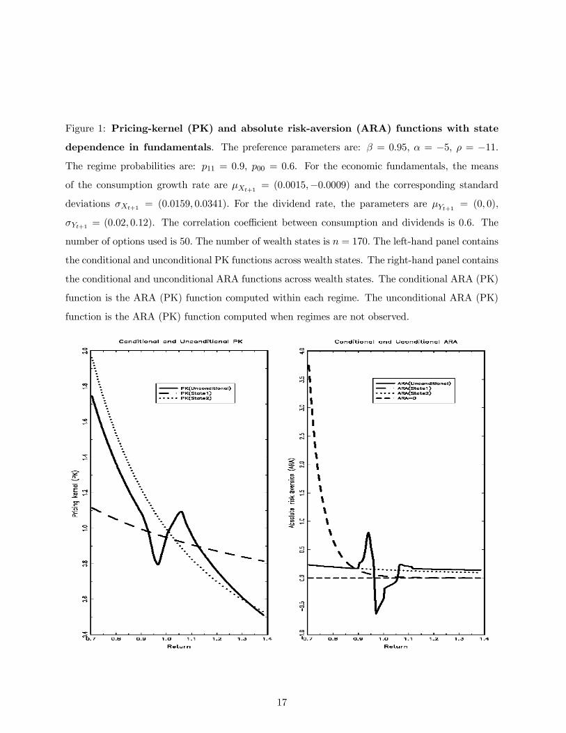
Figure 1: Pricing-kernel (PK) and absolute risk-aversion (ARA) functions with state
dependence in fundamentals. The preference parameters are: β = 0.95, α = −5, ρ = −11.The regime probabilities are: p11 = 0.9, p00 = 0.6. For the economic fundamentals, the means
of the consumption growth rate are µXt+1 = (0.0015,−0.0009) and the corresponding standarddeviations σXt+1 = (0.0159, 0.0341). For the dividend rate, the parameters are µYt+1 = (0, 0),
σYt+1 = (0.02, 0.12). The correlation coefficient between consumption and dividends is 0.6. The
number of options used is 50. The number of wealth states is n = 170. The left-hand panel contains
the conditional and unconditional PK functions across wealth states. The right-hand panel contains
the conditional and unconditional ARA functions across wealth states. The conditional ARA (PK)
function is the ARA (PK) function computed within each regime. The unconditional ARA (PK)
function is the ARA (PK) function computed when regimes are not observed.
17

Figure 2: Comparison of pricing-kernel (PK) and absolute risk-aversion (ARA) func-
tions with state dependence in fundamentals for two distance measures: The prefer-
ence parameters are: β = 0.95, α = −5, ρ = −11. The regime probabilities are: p11 = 0.9,
p00 = 0.6. For the economic fundamentals, the means of the consumption growth rate are
µXt+1 = (0.0015,−0.0009), and the corresponding standard deviations σXt+1 = (0.0159, 0.0341).
For the dividend rate, the parameters are µYt+1 = (0, 0), σYt+1 = (0.02, 0.12). The correlation coef-
ficient between consumption and dividends is 0.6. The number of options used is 50. The number of
wealth states is n = 170. The left-hand panel contains the unconditional PK function across wealth
states for the goodness-of-fit and the Hansen and Jagannathan (1997) distance measures. The
right-hand panel contains the unconditional ARA function across wealth states for the goodness-
of-fit and the Hansen and Jagannathan (1997) distance measures. The unconditional ARA (PK)
function is the ARA (PK) function computed when regimes are not observed.
18

Figure 3: Pricing-kernel (PK) and absolute risk-aversion (ARA) functions with state
dependence in preferences. The preference parameters are β = 0.95, α = (−7,−4.8), ρ = −10.The regime probabilities are p11 = 0.9, p00 = 0.6. For the economic fundamentals, the mean of
the consumption growth rate is µXt+1 = 0.018 and the standard deviation σXt+1 = 0.037. For the
dividend rate, Yt+1, the parameters are µYt+1 = −0.0018 , σYt+1 = 0.12. The correlation coefficientbetween consumption and dividend is 0.6. The number of options used is 50. The number of
wealth states is n = 170. The left-hand panel contains the conditional and unconditional PK
functions across wealth states. The right-hand panel contains the conditional and unconditional
ARA functions across wealth states. The conditional ARA (PK) function is the ARA (PK) function
computed within each regime. The unconditional ARA (PK) function is the ARA (PK) function
computed when regimes are not observed.
19

Figure 4: Comparison of pricing-kernel (PK) and absolute risk-aversion (ARA) func-
tions with state dependence in preferences. The preference parameters are β = 0.97,
α = (−7,−4.8), ρ = −10. The regime probabilities are p11 = 0.9, p00 = 0.6. For the economic fun-damentals, the mean of the consumption growth rate is µXt+1 = 0.018 and the standard deviation
σXt+1 = 0.037. For the dividend rate, Yt+1, the parameters are µYt+1 = −0.0018 , σYt+1 = 0.12. Thecorrelation coefficient between consumption and dividend is 0.6. The number of options used is 50.
The number of wealth states is n = 170. The left-hand panel contains the unconditional ARA func-
tion across wealth states for the goodness-of-fit and the Hansen and Jagannathan (1997) distance
measures. The right-hand panel contains the unconditional ARA function across wealth states for
the goodness-of-fit and the Hansen and Jagannathan (1997) distance measures. The unconditional
ARA (PK) function is the ARA (PK) function computed when regimes are not observed.
20
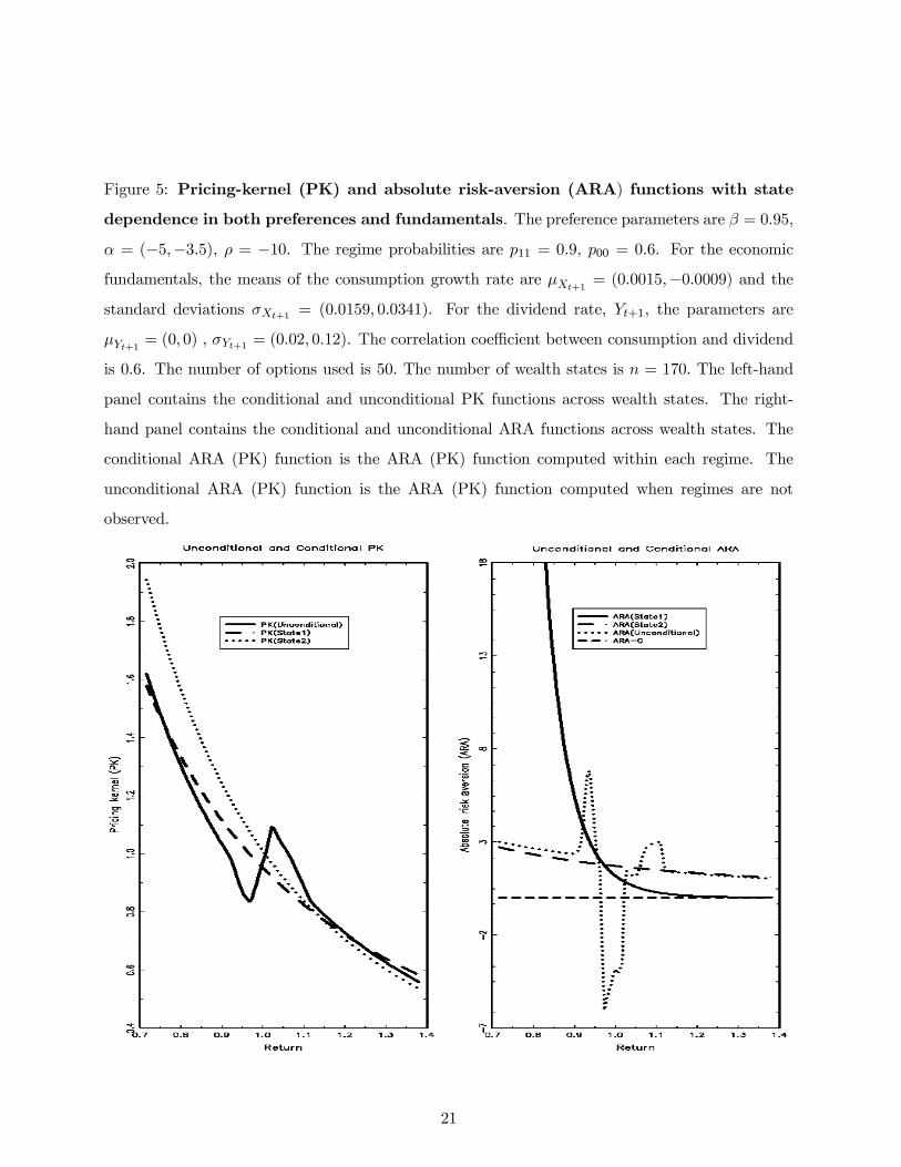
Figure 5: Pricing-kernel (PK) and absolute risk-aversion (ARA) functions with state
dependence in both preferences and fundamentals. The preference parameters are β = 0.95,
α = (−5,−3.5), ρ = −10. The regime probabilities are p11 = 0.9, p00 = 0.6. For the economic
fundamentals, the means of the consumption growth rate are µXt+1 = (0.0015,−0.0009) and thestandard deviations σXt+1 = (0.0159, 0.0341). For the dividend rate, Yt+1, the parameters are
µYt+1 = (0, 0) , σYt+1 = (0.02, 0.12). The correlation coefficient between consumption and dividend
is 0.6. The number of options used is 50. The number of wealth states is n = 170. The left-hand
panel contains the conditional and unconditional PK functions across wealth states. The right-
hand panel contains the conditional and unconditional ARA functions across wealth states. The
conditional ARA (PK) function is the ARA (PK) function computed within each regime. The
unconditional ARA (PK) function is the ARA (PK) function computed when regimes are not
observed.
21

Figure 6: Comparison of pricing-kernel (PK) and absolute risk-aversion (ARA) func-
tions with state dependence in both preferences and fundamentals. The preference
parameters are β = 0.95, α = (−5,−3.5), ρ = −10. The regime probabilities are p11 = 0.9,
p00 = 0.6. For the economic fundamentals, the means of the consumption growth rate are
µXt+1 = (0.0015,−0.0009) and the standard deviations σXt+1 = (0.0159, 0.0341). For the divi-
dend rate, Yt+1, the parameters are µYt+1 = (0, 0) , σYt+1 = (0.02, 0.12). The correlation coefficient
between consumption and dividend is 0.6. The number of options used is 50. The number of wealth
states is n = 170. The left-hand panel contains the unconditional PK function across wealth states
for the goodness-of-fit and Hansen and Jagannathan (1997) distance measures. The right-hand
panel contains the unconditional ARA function across wealth states for the goodness-of-fit and
Hansen and Jagannathan (1997) distance measures. The unconditional ARA (PK) function is the
ARA (PK) function computed when regimes are not observed.
22

App endi x: Pro of of Prop osi t i on 3. 2
P P 3.2. Rearranging equation (6.9) for the pricing kernel in Melino and
Yang (2003), one obtains:
mt+1 =
β (Ut) Ct+1Ct
ρ(Ut)− ρ(Ut)
ρ(Ut+1)
γ(Ut)R α(Ut)
ρ(Ut+1)−1
mt+1 P
α(Ut)
ρ(Ut+1)−α(Ut)
ρ(Ut)
t ,
where γ (Ut) =α(Ut)ρ(Ut)
and Pt is the equilibrium price of the market portfolio at time t. If ρ (Ut) =
ρ (Ut+1) and β (Ut) , α (Ut) , ρ (Ut) are constants, this pricing kernel reduces to the Epstein and
Zin (1989) pricing kernel. Let ϕ (Ut) = StDtdenote the price-dividend ratio and λ (Ut) =
PtCtthe
price-earnings ratio. The return on the market portfolio can be written as
Rmt+1 =Pt+1 +Ct+1
Pt=
λ U t+11 + 1
λ (Ut)
Ct+1Ct
,
and the stock return:St+1St
=ϕ U t+11
ϕ (Ut)
Dt+1Dt
.
Let us assume that the conditional probability distribution of log Ct+1Ct, log Dt+1Dt
, given U t+11 , is
a bivariate normal: log Ct+1Ct
log Dt+1Dt
/UT1 N
µXt+1
µYt+1
, σ2Xt+1 σXY,t+1
σXY,t+1 σ2Yt+1
, (A.1)
with U t+11 = (Uτ )1≤τ≤t+1. Taking the logarithm of mt+1, we get
logmt+1 = γ (Ut) log β (Ut) +α (Ut)
ρ (Ut+1)− 1 log
λ U t+11 + 1
λ (Ut)+
α (Ut)
ρ (Ut+1)− α (Ut)
ρ (Ut)log (λ (Ut)Ct) +
γ (Ut) ρ (Ut)− ρ (Ut)
ρ (Ut+1)+
α (Ut)
ρ (Ut+1)− 1 log
Ct+1Ct
.
The logarithm of the stock return is
logSt+1St
= logϕ U t+11
ϕ (Ut)+ log
Dt+1Dt
.
Consequently, logmt+1log St+1St
= A+B log Ct+1Ct
log Dt+1Dt
,23

where A = (a1, a2) with
a1 = γ (Ut) log β (Ut) + ρ (Ut)− ρ (Ut)
ρ (Ut+1)log
λ U t+11 + 1
λ (Ut)+
α (Ut)
ρ (Ut+1)− α (Ut)
ρ (Ut)log (λ (Ut)Ct) ,
a2 = logϕ U t+11
ϕ (Ut),
and B is a diagonal matrix with diagonal coefficients:
b11 = γ (Ut) ρ (Ut)− ρ (Ut)
ρ (Ut+1)+
α (Ut)
ρ (Ut+1)− 1 .
b22 = 1.
Using (A.1), it is straightforward to show that: logmt+1log St+1St
/U t+11 N [µ,Σms] ,
with
µ = A+B
µXt+1
µYt+1
,Σms = B
σ2Xt+1 σXt+1Yt+1
σXt+1Yt+1 σ2Yt+1
B.This completes the proof.
24

Bank of Canada Working PapersDocuments de travail de la Banque du Canada
Working papers are generally published in the language of the author, with an abstract in both officiallanguages.Les documents de travail sont publiés généralement dans la langue utilisée par les auteurs; ils sontcependant précédés d’un résumé bilingue.
Copies and a complete list of working papers are available from:Pour obtenir des exemplaires et une liste complète des documents de travail, prière de s’adresser à:
Publications Distribution, Bank of Canada Diffusion des publications, Banque du Canada234 Wellington Street, Ottawa, Ontario K1A 0G9 234, rue Wellington, Ottawa (Ontario) K1A 0G9E-mail: [email protected] Adresse électronique : [email protected] site: http://www.bankofcanada.ca Site Web : http://www.banqueducanada.ca
20052005-8 Recent Developments in Self-Employment in Canada N. Kamhi and D. Leung
2005-7 Determinants of Borrowing Limits on Credit Cards S. Dey and G. Mumy
2005-6 Monetary Policy under Model and Data-Parameter Uncertainty G. Cateau
2005-5 Y a-t-il eu surinvestissement au Canada durant la seconde moitiédes années 1990? S. Martel
2005-4 State-Dependent or Time-Dependent Pricing:Does It Matter for Recent U.S. Inflation? P.J. Klenow and O. Kryvtsov
2005-3 Pre-Bid Run-Ups Ahead of Canadian Takeovers:How Big Is the Problem? M.R. King and M. Padalko
2005-2 The Stochastic Discount Factor: Extending the VolatilityBound and a New Approach to Portfolio Selection withHigher-Order Moments F. Chabi-Yo, R. Garcia, and E. Renault
2005-1 Self-Enforcing Labour Contracts and the Dynamics Puzzle C. Calmès
20042004-49 Trade Credit and Credit Rationing in
Canadian Firms R. Cunningham
2004-48 An Empirical Analysis of the Canadian TermStructure of Zero-Coupon Interest Rates D.J. Bolder, G. Johnson, and A. Metzler
2004-47 The Monetary Origins of Asymmetric Informationin International Equity Markets G.H. Bauer and C. Vega
2004-46 Une approche éclectique d’estimation du PIBpotentiel pour le Royaume-Uni C. St-Arnaud
2004-45 Modelling the Evolution of Credit Spreadsin the United States S.M. Turnbull and J. Yang
2004-44 The Transmission of World Shocks toEmerging-Market Countries: An Empirical Analysis B. Desroches


