
Appendix A. Process Document
Memorandum of Understanding (MOU) Between SCAG and Gateway Cities Council of Governments for the Gateway Cities Sustainable Communities Strategy, October 7, 2010
Exhibit A. SCAG Framework and Guidelines for Subregional Sustainable Communities Strategy, April 1, 2010

Southern California Association of Governments
(Approved by Regional Council - April 1, 2010)
FRAMEWORK AND GUIDELINES for
SUBREGIONAL SUSTAINABLE COMMUNITIES STRATEGY I. INTRODUCTION
SB 375 (Steinberg), also known as California’s Sustainable Communities Strategy and Climate Protection Act, is a new state law which became effective January 1, 2009. SB 375 calls for the integration of transportation, land use, and housing planning, and also establishes the reduction of greenhouse gas (GHG) emissions as one of the main goals for regional planning. SCAG, working with the individual County Transportation Commissions (CTCs) and the subregional organizations within the SCAG region, is responsible for implementing SB 375 in the Southern California region. Success in this endeavor is dependent on collaboration with a range of public and private partners throughout the region.
Briefly summarized here, SB 375 requires SCAG as the Metropolitan Planning Organization to:
Prepare a Sustainable Communities Strategy (SCS) as part of the 2012 Regional Transportation Plan (RTP). The SCS will meet a State-determined regional GHG emission reduction target, if it is feasible to do so.
Prepare an Alternative Planning Strategy (APS) that is not part of the RTP if the SCS is unable to meet the regional target.
Integrate SCAG planning processes, in particular assuring that the Regional Housing Needs Assessment (RHNA) is consistent with the SCS, at the jurisdiction level.
Specific to SCAG only, allow for subregional SCS/APS development. Develop a substantial public participation process involving all stakeholders.
Unique to the SCAG region, SB 375 provides that “a subregional council of governments and the county transportation commission may work together to propose the sustainable communities strategy and an alternative planning strategy . . . for that subregional area.” Govt. Code §65080(b)(2)(C). In addition, SB 375 authorizes that SCAG “may adopt a framework for a subregional SCS or a subregional APS to address the intraregional land use, transportation, economic, air quality, and climate policy relationships.” Id. Finally, SB 375 requires SCAG to “develop overall guidelines, create public participation plans, ensure coordination, resolve conflicts, make sure that the overall plan complies with applicable legal requirements, and adopt the plan for the region.” Id. The intent of this Framework and Guidelines for Subregional Sustainable Communities Strategy (also referred to herein as the “Framework and Guidelines” or the “Subregional Framework and Guidelines”) is to offer the SCAG region’s subregional agencies the highest degree of autonomy,
2
flexibility and responsibility in developing a program and set of implementation strategies for their subregional areas. This will allow the subregional strategies to better reflect the issues, concerns, and future vision of the region’s collective jurisdictions with the input of the fullest range of stakeholders. In order to achieve these objectives, it is necessary for SCAG to develop measures that assure equity, consistency and coordination, such that SCAG can incorporate the subregional SCSs in its regional SCS which will be adopted as part of the 2012 RTP pursuant to SB 375. For that reason, this Framework and Guidelines establishes standards for the subregion’s work in preparing and submitting subregional strategies, while also laying out SCAG’s role in facilitating and supporting the subregional effort with data, tools, and other assistance. While the Framework and Guidelines are intended to facilitate the specific subregional option to develop the SCS (and APS if necessary) as described in SB 375, SCAG encourages the fullest possible participation from all subregional organizations. As SCAG undertakes implementation of SB 375 for the first time, SCAG has also designed a “collaborative” process, in cooperation with the subregions, that allows for robust subregional participation for subregions that choose not to exercise their statutory option. II. ELIGIBILITY AND PARTICIPATION SB 375 allows for subregional councils of governments in the SCAG region to have the option to develop the SCS (and the APS if necessary) for their area. SCAG interprets this option as being available to any subregional organization recognized by SCAG, regardless of whether the organization is formally established as a “subregional council of governments.” County Transportation Commissions (CTCs) play an important and necessary role in the development of a subregional SCS. Any subregion that chooses to develop a subregional strategy will need to work closely with the respective CTC in its subregional area in order to identify and integrate transportation projects and policies. Beyond working with CTCs, SCAG encourages partnership efforts in the development of subregional strategies, including partnerships between and among subregions. Subregional agencies must formally indicate to SCAG, in writing, by December 31, 2009 if they intend to exercise this option to develop their own SCS. Subregions that choose to develop an SCS for their area must do so in a manner consistent with this Framework and Guidelines. The subregion’s intent to exercise its statutory option to prepare the strategy for their area must be decided and communicated through formal action of the subregional agency’s governing board. Subsequent to receipt of any subregion’s intent to develop and adopt an SCS, SCAG will convene discussions regarding a formal written agreement between SCAG and the subregion, which may be revised if necessary, as the SCS process is implemented. III. FRAMEWORK The Framework portion of this document covers regional objectives and policy considerations, and provides general direction to the subregions in preparing their own SCS, and APS if necessary.

3
A. SCAG’s preliminary goals for implementing SB 375 are as follows:
o Achieve the regional GHG emission reduction target for cars and light trucks through an SCS. o Fully integrate SCAG’s planning processes for transportation, growth, intergovernmental
review, land use, housing, and the environment. o Seek areas of cooperation that go beyond the procedural statutory requirements, but that also
result in regional plans and strategies that are mutually supportive of a range of goals. o Build trust by providing an interactive, participatory and collaborative process for all
stakeholders. Provide, in particular, for the robust participation of local jurisdictions, subregions and CTCs in the development of the SCAG regional SCS and implementation of the subregional provisions of the law.
o Assure that the SCS adopted by SCAG and submitted to California Air Resources Board (ARB) is a reflection of the region’s collective growth strategy and vision for the future.
o Develop strategies that incorporate and are respectful of local and subregional priorities, plans, and projects.
B. Flexibility Subregions may develop any appropriate strategy to address the region’s greenhouse gas reduction goals and the intent of SB 375. While subregions will be provided with SCAG data, and with a conceptual or preliminary scenario to use as a helpful starting point, they may employ any combination of land use policy change, transportation policy, and transportation investment, within the specific parameters described in the Guidelines. C. Outreach Effort and Principles Subregions are required to conduct an open and participatory process that includes the fullest possible range of stakeholders. As further discussed within the Guidelines, SCAG amended its existing Public Participation Plan (PPP) to describes SCAG’s responsibilities in complying with the outreach requirements of SB 375 and other applicable laws and regulations. SCAG will fulfill its outreach requirements for the regional SCS/APS which will include outreach activities regarding the subregional SCS/APS. Subregions are also encouraged to design their own outreach process that meets each subregion’s own needs and reinforces the spirit of openness and full participation. To the extent that subregions do establish their own outreach process, this process should be coordinated with SCAG’s outreach process. D. Communication and Coordination Subregions developing their own SCS are strongly encouraged to maintain regular communication with SCAG staff, the respective CTC, their jurisdictions and other stakeholders, and other subregions if necessary, to review issues as they arise and to assure close coordination. Mechanisms for on-going communication should be established in the early phases of strategy development. E. Planning Concepts SCAG, its subregions, and member cities have established a successful track record on a range of land use and transportation planning approaches through the on-going SCAG Compass Blueprint Program, including approximately 60 local demonstration projects completed to date. Subregions are
4
encouraged to capture, further develop and build off the concepts and approaches of the Compass Blueprint program. In brief, these include developing transit-oriented, mixed use, and walkable communities, and providing for a mix of housing and jobs. IV. GUIDELINES These Guidelines describe specific parameters for the subregional SCS/APS effort under SB 375, including process, deliverables, data, documentation, and timelines. As described above, the Guidelines are created to ensure that the region can successfully incorporate strategies developed by the subregions into the regional SCS, and that the region can comply with its own requirements under SB 375. Failure to proceed in a manner consistent with the Guidelines will result in SCAG not accepting a subregion’s submitted strategy. A. Subregional Process (1) Subregional Sustainable Communities Strategy Subregions that choose to exercise their optional role under SB 375 will develop and adopt a subregional Sustainable Communities Strategy. That strategy must contain all of the required elements, and follow all procedures, as described in SB 375. Subregions may choose to further develop an Alternative Planning Strategy (APS), according to the procedures and requirements described in SB 375. If subregions prepare an APS, they must prepare a Sustainable Communities Strategy first, in accordance with SB 375. A subregional APS is not “in lieu of” a subregional SCS, but in addition to the subregional SCS. In part, an APS must identify the principal impediments to achieving the targets within the SCS. The APS must show how the GHG emission targets would be achieved through alternative development patterns, infrastructure, and additional transportation measures or policies. SCAG encourages subregions to focus on feasible strategies that can be included in the SCS. The subregional SCS must include all components of a regional SCS as described in SB 375, and outlined below:
(i.) identify the general location of uses, residential densities, and building intensities within the
subregion; (ii.) identify areas within the subregion sufficient to house all the population of the subregion,
including all economic segments of the population, over the course of the planning period of the RTP taking into account net migration into the region, population growth, household formation and employment growth;
(iii.) identify areas within the subregion sufficient to house an eight-year projection of the regional housing need for the subregion pursuant to Section 65584;
(iv.) identify a transportation network to service the transportation needs of the subregion; (v.) gather and consider the best practically available scientific information regarding resource
areas and farmland in the subregion as defined in subdivisions (a) and (b) of Section 65080.01;
(vi.) consider the state housing goals specified in Sections 65580 and 65581; (vii.) set forth a forecasted development pattern for the subregion, which, when integrated with the
transportation network, and other transportation measures and policies, will reduce the greenhouse gas emissions from automobiles and light trucks to achieve, if there is a feasible way to do so, the greenhouse gas emission reduction targets approved by the ARB; and

5
(viii.) allow the RTP to comply with Section 176 of the federal Clean Air Act (42 U.S.C. Sec. 7506). See, Government Code §65080(b)(2)(B).
In preparing the subregional SCS, the subregion will consider feasible strategies, including local land use policies, transportation infrastructure investment (e.g., transportation projects), and other transportation policies such as Transportation Demand Management (TDM) strategies (which includes pricing), and Transportation System Management (TSM) strategies. Technological measures may be included if they exceed measures captured in other state and federal requirements (e.g., AB32). As discussed further below (under “Documentation”), subregions need not constrain land use strategies considered for the SCS to current General Plans. In other words, the adopted strategy need not be fully consistent with local General Plans currently in place. However, should the adopted subregional strategy deviate from General Plans, subregions will need to demonstrate the feasibility of the strategy by documenting any affected jurisdictions’ willingness to adopt the necessary General Plan changes. The regional SCS shall be part of the 2012 RTP. Therefore, for transportation investments included in a subregional SCS to be valid, they must also be included in the 2012 RTP. Further, such projects need to be scheduled in the RTIP for construction completion by the target years (2020 and 2035) in order to demonstrate any benefits as part of the SCS. As such, subregions will need to collaborate with the respective CTC in their area to coordinate the subregional SCS with future transportation investments. It should also be noted that the California Transportation Commission is updating their RTP Guidelines. This topic is likely to be part of further discussion through the SCS process as well. SCAG will accept and incorporate the subregional SCS, unless (a) it does not comply with SB 375, (b) it is does not comply with federal law, or (c) it is does not comply with SCAG’s Subregional Framework and Guidelines. In the event that a compiled regional SCS, including subregional submissions, does not achieve the regional target, SCAG will initiate a process to develop and consider additional GHG emission reduction measures region-wide. SCAG will develop a written agreement with each subregional organization to define a process and timeline whereby subregions would submit a draft subregional SCS for review and comments to SCAG, so that any inconsistencies may be identified and resolved early in the process. Furthermore, SCAG will compile and disseminate performance information on the preliminary regional SCS and its components in order to facilitate regional dialogue. The development of a subregional SCS does not exempt any subregion from further GHG emission reduction measures being included in the regional SCS. Further, all regional measures needed to meet the regional target will be subject to adoption by the Regional Council, and any additional subregional measures beyond the SCS submittal from subregions accepting delegation needed to meet the regional target must also be adopted by the subregional governing body. (2) Subregional Alternative Planning Strategy (APS) Subregions are encouraged to focus their efforts on feasible measures that can be included in an SCS. In the event that a subregion chooses to prepare an APS, the content of a subregional APS should be consistent with what is required by SB 375 (see, Government Code §65080(b)(2)(H)), as follows:
(i.) Shall identify the principal impediments to achieving the subregional SCS.
6
(ii.) May include an alternative development pattern for the subregion pursuant to subparagraphs (B) to (F), inclusive.
(iii.) Shall describe how the alternative planning strategy would contribute to the regional greenhouse gas emission reduction target, and why the development pattern, measures, and policies in the alternative planning strategy are the most practicable choices for the subregion.
(iv.) An alternative development pattern set forth in the alternative planning strategy shall comply with Part 450 of Title 23 of, and Part 93 of Title 40 of, the Code of Federal Regulations, except to the extent that compliance will prevent achievement of the regional greenhouse gas emission reduction targets approved by the ARB.
(v.) For purposes of the California Environmental Quality Act (Division 13 (commencing with Section 21000) of the Public Resources Code), an alternative planning strategy shall not constitute a land use plan, policy, or regulation, and the inconsistency of a project with an alternative planning strategy shall not be a consideration in determining whether a project may have an environmental effect.
Any precise timing or submission requirements for a subregional APS will be determined based on further discussions with subregional partners. As previously noted, a subregional APS is in addition to a subregional SCS.
(3) Outreach and Process
SCAG will fulfill all of its outreach requirements under SB 375 for the regional SCS/APS, which will include outreach regarding any subregional SCS/APS. SCAG staff has revised its Public Participation Plan to incorporate the outreach requirements of SB 375, and integrate the SB 375 process with the 2012 RTP development as part of SCAG’s Public Participation Plan Amendment No. 2, adopted by SCAG’s Regional Council on December 3, 2009. Subsequent to the adoption of the PPP Amendment No. 2, SCAG will continue to discuss with subregions and stakeholders the Subregional Framework & Guidelines, which further describe the Public Participation elements of SB 375.
Subregions that elect to prepare their own SCS or APS are encouraged to present their subregional SCS or APS, in coordination with SCAG, at all meetings, workshops and hearings held by SCAG in their respective counties. Additionally, the subregions would be asked to either provide SCAG with their mailing lists so that public notices and outreach materials may also be posted and sent out by SCAG, or SCAG will provide notices and outreach materials to the subregions for their distribution to stakeholders. The SCAG PPP Amendment No. 2 provides that additional outreach may be performed by subregions. Subregions are strongly encouraged to design and adopt their own outreach processes that mimic the specific requirements imposed on the region under SB 375. Subregional outreach processes should reinforce the regional goal of full and open participation, and engagement of the broadest possible range of stakeholders.
(4) Subregional SCS Approval
It is recommended that the governing board of the subregional agency approve the subregional SCS prior to submission to SCAG. While the exact format is still subject to further discussion, SCAG recommends that there be a resolution from the governing board of the subregion with a finding that the land use strategies included in the subregional SCS are feasible and based upon consultation with the local jurisdictions in the respective subregion. Subregion should consult with their legal counsel as to compliance with the California Environmental Quality Act (CEQA). In SCAG’s view, the

7
subregional SCS is not a “project” for the purposes of CEQA; rather, the 2012 RTP which will include the regional SCS is the actual “project” which will be reviewed for environmental impacts pursuant to CEQA. As such, the regional SCS, which will include the subregional SCSs, will undergo a thorough CEQA review. Nevertheless, subregions approving subregional SCSs should consider issuing a notice of exemption under CEQA to notify the public of their “no project” determination and/or to invoke the “common sense” exemption pursuant to CEQA Guidelines § 15061(b)(3).
Finally, in accordance with SB 375, subregions are strongly encouraged to work in partnership with the CTC in their area. SCAG can facilitate these arrangements if needed.
(5) Data Standards SCAG is currently assessing the precise data standards anticipated for the regional and subregional SCS. In particular, SCAG is reviewing the potential use of parcel data and development types currently used for regional planning. At present, the following describes the anticipated data requirements for a subregional SCS. 1. Types of Variables
Variables are categorized into socio-economic variables and land use variables. The socio-economic variables include population, households, housing units, and employment. The land use variables include land uses, residential densities, building intensities, etc, as described in SB 375.
2. Geographical Levels
SCAG is considering the collection and adoption of the data at a small-area level as optional for local agencies in order to make accessible the CEQA streamlining provisions under SB 375. The housing unit, employment, and the land use variables can be collected at a small-area level for those areas which under SB 375 qualify as containing a “transit priority project” (i.e. within half-mile of a major transit stop or high-quality transit corridor) for purposes of allowing jurisdictions to take advantage of the CEQA streamlining incentives in SB 375.
For all other areas in the region, SCAG staff will collect the population, household, employment, and land use variables at the Census tract or Traffic Analysis Zone (TAZ) level.
3. Base Year and Forecast Years
The socio-economic and land use variables will be required for the base year of 2008, and the target years of 2020 and 2035.
(6) Documentation Subregions are expected to maintain full and complete records related to the development of the subregional SCS, including utilizing the most recent planning assumptions considering local general plans and other factors. In particular, subregions must document the feasibility of the subregional strategy by demonstrating the willingness of local agencies to consider and adopt land use changes necessitated by the SCS. The format for this documentation may include adopted resolutions from local jurisdictions and/or the subregion’s governing board.

8
(7) Timing An overview schedule of the major milestones of the subregional process and its relationship to the regional SCS/RTP is included below. Subregions must submit the subregional SCS to SCAG by the date prescribed. Further, SCAG will need a preliminary SCS from subregions for the purpose of preparing a project description for the 2012 RTP Program Environmental Impact Report. The precise content of this preliminary submission will be determined based on further discussions. The anticipated timing of this preliminary product is approximately February 2011. (8) Relationship to Regional Housing Needs Assessment (RHNA) and Housing Element
Although SB 375 calls for an integrated process, subregions are not automatically required to take on RHNA delegation as described in State law if they prepare an SCS/APS. However, SCAG encourages subregions to undertake both processes due to their inherent connections.
SB 375 requires that the RHNA allocated housing units be consistent with the development pattern included in the SCS. See, Government Code §65584.04(i). Population and housing demand must also be proportional to employment growth. At the same time, in addition to the requirement that the RHNA be consistent with the development pattern in the SCS, the SCS must also identify areas that are sufficient to house the regional population by income group through the RTP planning period, and must identify areas to accommodate the region’s housing need for the next local Housing Element eight year planning period update. The requirements of the statute are being further interpreted through the RTP guidelines process. Staff intends to monitor and participate in the guideline process, inform stakeholders regarding various material on these issues, and amend, if necessary, these Framework and Guidelines, pending its adoption.
SCAG will be adopting the RHNA and applying it to local jurisdictions at the jurisdiction boundary level. SCAG staff believes that consistency between the RHNA and the SCS may still be accomplished by aggregating the housing units contained in the smaller geographic levels noted in the SCS and including such as part of the total jurisdictional number for RHNA purpose. SCAG staff has concluded that there is no consistency requirement for RHNA purposes at sub-jurisdictional level, even though the SCS is adopted at the smaller geographic level for the opportunity areas. The option to develop a subregional SCS is separate from the option for subregions to adopt a RHNA distribution, and subject to separate statutory requirements. Nevertheless, subregions that develop and adopt a subregional SCS should be aware that the SCS will form the basis for the allocation of housing need as part of the RHNA process. Further, SCS development requires integration of elements of the RHNA process, including assuring that areas are identified to accommodate the 8 year need for housing, and that housing not be constrained by certain types of local growth controls as described in State law. SCAG will provide further guidance for subregions and a separate process description for the RHNA.
B. COUNTY TRANSPORTATION COMMISSIONS’ ROLES AND RESPONSIBLITIES Subregions that develop a subregional SCS will need to work closely with the CTCs in their area in order to coordinate and integrate transportation projects and policies as part of the subregional SCS. As discussed above (under “Subregional Sustainable Communities Strategy”), any transportation

9
projects identified in the subregional SCS must also be included in the 2012 RTP in order to be considered as a feasible strategy. SCAG can help to facilitate communication between subregions and CTCs. C. SCAG ROLES AND RESPONSIBLITIES SCAG’s roles in supporting the subregional SCS development process are in the following areas: (1) Preparing and adopting the Framework and Guidelines SCAG will adopt these Framework and Guidelines in order to assure regional consistency and the region’s compliance with law. (2) Public Participation Plan SCAG will assist the subregions by developing, adopting and implementing a Public Participation Plan and outreach process with stakeholders. This process includes consultation with congestion management agencies, transportation agencies, and transportation commissions; and SCAG will hold public workshops and hearings. SCAG will also conduct informational meetings in each county within the region for local elected officials (members of the board of supervisors and city councils), to present the draft SCS, and APS if necessary, and solicit and consider input and recommendations. (3) Methodology As required by SB 375, SCAG will adopt a methodology for measuring greenhouse gas emission reductions associated with the strategy. (4) Incorporation/Modification
SCAG will accept and incorporate the subregional SCS unless it does not comply with SB 375, federal law, or the Subregional Framework and Guidelines. As SCAG intends the entire SCS development process to be iterative, SCAG will not amend a locally-submitted SCS. SCAG may provide additional guidance to subregions so that subregions may make amendments to its subregional SCS as part of the iterative process, or request a subregion to prepare an APS if necessary. Further, SCAG can propose additional regional strategies if feasible and necessary to achieve the regional emission reduction target with the regional SCS. SCAG will develop a written agreement with each subregional organization to define a process and timeline whereby subregions would submit a draft subregional SCS for review and comments to SCAG, so that any inconsistencies may be identified and resolved early in the process.
(5) Modeling
SCAG currently uses a Trip-Based Regional Transportation Demand Model and ARB’s EMFAC model for emissions purposes. In addition to regional modeling, SCAG is developing tools to evaluate the effects of strategies that are not fully accounted for in the regional model. SCAG is also developing two additional tools – a Land Use Model and an Activity Based Model – to assist in strategy development and measurement of outcomes under SB 375.

10
In addition to modeling tools which are used to measure results of completed scenarios, SCAG is developing a scenario planning tool for use in workshop settings as scenarios are being created with jurisdictions and stakeholders. The tool will be made available to subregions and local governments for their use in subregional strategy development.
(6) Adoption/Submission to State
After the incorporation of subregional strategies, SCAG will finalize and adopt the regional SCS as part of the 2012 RTP. SCAG will submit the SCS to ARB for review as required in SB 375.
(7) Conflict Resolution
While SB 375 requires SCAG to develop a process for resolving conflicts, it is unclear at this time the nature or purpose of a conflict resolution process as SCAG does not intend to amend a locally-submitted SCS. As noted above, SCAG will accept the subregional SCS unless it is inconsistent with SB 375, federal law, or the Subregional Framework and Guidelines. SCAG will also request that a subregion prepare an APS if necessary. It is SCAG’s intent that the process be iterative and that there be coordination among SCAG, subregions and their respective jurisdictions and CTCs. SCAG is open to further discussion on issues which may generate a need to establish a conflict resolution process as part of the written agreement between SCAG and the subregional organization.
(8) Funding Funding for subregional activities is not available at this time, and any specific parameters for future funding are speculative. Should funding become available, SCAG anticipates providing a share of available resources to subregions. While there are no requirements associated with potential future funding at this time, it is advisable for subregions to track and record their expenses and activities associated with these efforts. (9) Preliminary Scenario Planning SCAG will work with each subregion to collect information and prompt dialogue with each local jurisdiction prior to the start of formal SCS development. This phase of the process is identified as “preliminary scenario planning” in the schedule below. The purpose of this process is to create a base of information to inform SCAG’s recommendation of a regional target to ARB prior to June 2010. All subregions are encouraged to assist SCAG in facilitating this process. (10) Data SCAG is currently developing, and will provide each subregion with datasets for the following:
(1) 2008 Base year; (2) General Plan/Growth projection & distribution; (3) Trend Baseline; and (4) Policy Forecast/SCS.
While the Trend Baseline is a technical projection that provides a best estimate of future growth based on past trends and assumes no general plan land use policy changes, the Policy Forecast/ SCS is derived using local input through a bottom-up process, reflecting regional policies including transportation investments. Local input is collected from counties, subregions, and local jurisdictions.

11
Data/GIS maps will be provided to subregions and local jurisdiction for their review. This data and maps include the 2008 base year socioeconomic estimates and 2020 and 2035 socioeconomic forecast. Other GIS maps including the existing land use, the general plan land use, the resource areas, and other important areas identified in SB 375. It should be noted that none of the data/ maps provided were endorsed or adopted by SCAG’s Community, Economic and Human Development Committee (CEHD). All data/maps provided are for the purpose of collecting input and comments from subregions and local jurisdictions. This is to initiate dialogue among stakeholders to address the requirements of SB 375 and its implementation. The list of data/GIS maps include: 1. Existing land use 2. Zoning 3. General plan land use 4. Resource areas include:
(a.) all publicly owned parks and open space; (b.) open space or habitat areas protected by natural community conservation plans, habitat
conservation plans, and other adopted natural resource protection plans; (c.) habitat for species identified as candidate, fully protected, sensitive, or species of special
status by local, state, or federal agencies or protected by the federal Endangered Species Act (1973), the California Endangered Species Act, or Native Plant Protection Act;
(d.) lands subject to conservation or agricultural easements for conservation or agricultural purposes by local governments, special districts, or nonprofit 501(c)(3) organizations, areas of the state designated by the State Mining and Geology Board as areas of statewide or regional significance pursuant to Section 2790 of the Public Resources Code, and lands under Williamson Act contracts;
(e.) areas designated for open-space or agricultural uses in adopted open-space elements or agricultural elements of the local general plan or by local ordinance;
(f.) areas containing biological resources as described in Appendix G of the CEQA Guidelines that may be significantly affected by the sustainable communities strategy or the alternative planning strategy; and
(g.) an area subject to flooding where a development project would not, at the time of development in the judgment of the agency, meet the requirements of the National Flood Insurance Program or where the area is subject to more protective provisions of state law or local ordinance.
5. Farmland 6. Sphere of influence 7. Transit priority areas 8. City/Census tract boundary with ID 9. City/TAZ boundary with ID (11) Tools SCAG is developing a Local Sustainability Planning Model (LSPM) for subregions/local jurisdictions to analyze land use impact. The use of this tool is not mandatory and is at the discretion of the Subregion. The LSPM is a web-based tool that can be used to analyze, visualize and calculate the impact of land use changes on auto ownership, mode use, vehicle miles of travel (VMT), and greenhouse gas emissions in real time. Users will be able to estimate transportation and emissions impacts by modifying land use designations within their community.
12
Other tools currently maintained by SCAG may be useful to the subregional SCS development effort, including the web-based CaLOTS application. SCAG will consider providing guidance and training on additional tools based on further discussions with subregional partners. (12) Resources and technical assistance SCAG will assist the subregions by making available technical tools for scenario development as described above. Further, SCAG will assign a staff liaison to each subregion, regardless of whether the subregion exercises its statutory option to prepare an SCS. SCAG staff can participate in subregional workshops, meetings, and other processes at the request of the subregion, and pending funding and availability. SCAG’s legal staff will be available to assist with questions related to SB 375 or SCAG’s implementation of SB 375. Further, SCAG will prepare materials for its own process in developing the regional SCS, and will make these materials available to subregions. D. MILESTONES/SCHEDULE CARB issues Final Regional Targets – September 2010 SCS development (preliminary scenario, draft, etc) – through early 2011 Release Draft RTP/regional SCS for public review – November 2011 Regional Council adopts RTP/SCS – April 2012
If other milestones are needed, they will be incorporated into the written agreement between SCAG and the Subregion.
13

14

15

16

17

18

19
20

21

22

23
24

25

26

27

28
29
30

31

32

33

34

35

36

Appendix B. Prior Studies of the Gateway Cities Council of Governments Relevant to SB 375
PRIOR STUDIES OF THE
GATEWAY CITIES COUNCIL OF GOVERNMENTS RELEVANT TO SB375

Table of Contents Background/Introduction ................................................................................................. 1 Community Link 21: Southern California Association of Governments (SCAG’s) Draft Regional Transportation Plan .......................................................................................... 2 Livable Cities Case Studies ............................................................................................ 3 OrangeLine Feasibility Study .......................................................................................... 4 Supplemental Southeast Area Bus Restructuring Study ................................................ 5 The Gateway Cities Council of Governments Sub-Regional Housing Implementation Strategy ........................................................................................................................... 6 Gateway Cities Infrastructure Needs Assessment ......................................................... 6 I-710 Tier 2 Community Advisory Committee Final Report ............................................. 7 I-710 Oversight Policy Committee Adopted Locally Preferred Strategy .......................... 8 Gateway Cities COG – Summary of the Proceedings of the Joint Housing Summit “Strategies and Tactics for Infill Development Success” ................................................. 9 SR-91 / I-605 Needs Assessment Study ......................................................................... 9 The Gateway Cities & Surrounding Areas Intelligent Transportation System (ITS) Research and Strategies For Transportation and Goods Movement Study .................. 10 SR-91 / I-605 / I-405 Proposal for Major Corridor Study and RSTIS Peer Review Presented by Gateway Cities COG ............................................................................... 11 Draft (Revised) Technical Scope of Work Southeast Los Angeles County SR-91 / I-605 / I-405 Freeway Corridors Major Corridor Study (MCS) ................................................ 12 Development of the Air Quality Action Plan for the I-710 Corridor ................................ 12 SR-91 / I-605 / I-405 Initial Corridors Studies ................................................................ 15 White Paper – Addressing the Requirements of SB 375 at the Sub-regional Level ...... 17

1
BACKGROUND/INTRODUCTION In mid-2010, the Gateway Cities Council of Governments (COG) retained a Cambridge Systematics led team to assist the COG with the development of a Sustainable Communites Strategy (SCS) for the Gateway Cities sub-region, in accordance with the requirements of SB 375. One of the initial tasks of the work program for the development of the SCS involved the review of prior COG studies. The purpose of this task was to review prior studies to identify Vehicle Miles Traveled/ Greenhouse Gas (VMT/GHG) reduction measures contained in these studies that could be included in SCS Strategy portfolios to be prepared for each city by Cambridge Systematics. Team member Willdan Engineering was charged with this task of compiling and reviewing the prior COG studies. Being proactive in addressing issues facing its sub-region, the Gateway Cities COG has generated a number of studies since its inception. The COG has conducted 37 studies since 1996, exclusive of addendums and supplements, and of these, 25 are germane to SB 375 and the development of the sub-regional SCS and/or Regional Housing Needs Assessment. On the pages that follow, the 16 reports that contained the most relevant measures or other information with regard to VMT/GHG reductions are discussed in the chronological order in which they were prepared. Each report is briefly summarized and any key findings/recommendations relevant to VMT/GHG reductions are listed.
2
Report: Community Link 21: Southern California Association of Governments (SCAG’s) Draft Regional Transportation Plan Date: February 1998 Summary: This report reviews SCAG’s draft Regional Transportation Plan (RTP) (Community Link 21), explains its significance for the Gateway Cities Sub-region, and makes recommendations as to what position the Gateway Cities COG should take with respect to these issues. Findings/Recommendations Relevant to GHG and VMT Reductions include:
Gateway Cities Goods Movement Network, a system of intersections and connecting arterials, should be accorded programmatic status by SCAG, similar to the Alameda Corridor East, and properly budgeted with regional funding;
endorse truck lanes on I-710 in concept only, subject to further review and clarification;
request SCAG to allocate funding in the RTP for grade crossing improvements in the Gateway Cities;
Gateway Cities COG should participate in any regional bus restructuring and smart shuttles studies to have adequate local control over route and service decisions;
LAX expansion should be subject to the Metropolitan Transportation Authority’s (MTA’s) Congestion Management Plan requirements;
Intelligent Transportation System technologies should be identified as a means to improve the efficient and safe movement of people and goods; and
Gateway Cities COG should request a reconfiguration of the RTP to support infrastructure improvements in the industrial core as opposed to funding for spread out development that increases the burden on meeting air quality requirements in increasing vehicle miles traveled.

3
Report: Livable Cities Case Studies Date: 2001 Summary: Three case studies are presented in this report to demonstrate the possibilities of creating a livable community through strategies of downtown revitalization, reuse of industrial lands, and streetscape improvements to arterial corridors. Alternatives and recommendations presented in each case study are intended to provide lessons that can be utilized by all member cities facing similar challenges. Alternatives and recommendations by city include:
1. The case study for the City of Artesia focused on revitalizing an existing downtown by incorporating a healthy mix of uses, utilizing building form, architectural details and design guidelines to showcase the unique qualities of the city. In addition, the case study showed how to utilize the current assets of the city to focus their redevelopment energy and use the vitality of the downtown to strengthen the structure of the city as a whole.
2. The case study for the City of Paramount focused on the redevelopment of underutilized industrial land to achieve a city structure based on a series of walk-able, mixed-use districts serving local residents. In addition, the case study addressed how to link these districts through the use of public transit and streetscape design.
3. The case study for the City of Pico Rivera focused on the revitalization of a commercial arterial through the use of streetscape enhancements and urban design recommendations. More specifically, the case study addressed how to handle the transformation of a large thoroughfare historically dominated by industrial truck traffic into a mixed-use boulevard that contributes to the overall structure and vitality of the city.
One of the greatest issues facing the case study cities of Artesia, Paramount and Pico Rivera, and of relevance to all of the Gateway Cities, is the shift in land use caused by the changing regional economy. As large-scale manufacturing becomes less relevant to local economies, the conversion of post-industrial land becomes a key opportunity for these otherwise built-out metropolitan areas. Study and analysis of regional trends, as well as an understanding of what is important to the community, can help to direct the reuse of this land. New uses should support current and anticipated future trends in both the economics of land use and allocation, and support the retail, civic, and residential structure necessary to create “livable cities”.

4
Findings/Recommendations Relevant to GHG and VMT Reductions include:
Increase utilization of underutilized industrial land to create mixed-use activity areas that are linked through public transportation;
Improve the vitality of the downtown by incorporating a mix of uses and through the use of building form, architectural details and design guidelines; and
Transform a traffic-ridden thoroughfare into a more pedestrian-friendly, mixed-use boulevard.
Report: OrangeLine Feasibility Study Date: 2002 Summary: The OrangeLine feasibility study is a financial, engineering and environmental assessment of an advanced technology, 30-33 mile high-speed transportation system operating along the former Pacific Electric “Red Car” land and adjoining corridors. This corridor extends from downtown Los Angeles to central Orange County. Results indicate that the OrangeLine transportation system can provide the required transportation improvements to support current and future development, and that it could be successfully built and operated without the need for significant government subsidies. It is anticipated that additional housing, office and retail development projects completed along the OrangeLine corridor by 2025 will accommodate an increased population of 8,000 people within a quarter mile of station areas and tens of thousands more in the surrounding area, as well as up to 125,000 additional jobs. This growth in population and employment will result in added trips per day in the corridor. In addition to providing a very high quality, non-polluting transportation service to over 46,000 daily riders by 2025, the OrangeLine will also divert an estimated number of daily riders to other transit modes, thus significantly reducing the traffic impacts of future growth. The OrangeLine is projected to reduce auto trips in the corridor compared to travel patterns that would exist if the OrangeLine were not built. Findings/Recommendations Relevant to GHG and VMT Reductions include:
reduce auto trips by providing an advanced technology high-speed transportation system along a transportation corridor linking Los Angeles with central Orange County; and

5
provide for higher intensity housing, office and retail development projects along this public transit corridor.
Report: Supplemental Southeast Area Bus Restructuring Study Date: 2003 Summary: The purpose of this study was to identify and evaluate opportunities to improve existing local and regional fixed-route bus transit services, transit facilities, and community-level transit and Para transit systems serving the Southeast study area. This study builds on the Southeast Area Bus Restructuring Study, completed in August 2000, with an increased focus on community-based services in the Southeast area. The study presented concrete recommendations for improving transit service within the Southeast study area. Findings/Recommendations Relevant to GHG and VMT Reductions include:
County should conduct a more detailed review and analysis of passenger trip-making patterns to determine whether current service area designations effectively match reasonable trip requests from County residents (i.e., review the destinations commonly served or commonly requested to identify destination-rich areas and to determine what fit or misfit may exist with current service area designation);
cross-jurisdictional trips should be provided when needed to enhance services and provide services more cost-effectively;
cities within the study area should view the gradual implementation and development of both city-specific and coordinated multi-jurisdictional transit projects as wholly interrelated and necessary to develop a cohesive transportation network in the Southeast; and
cities in the study area should establish a formalized institutional arrangement that is easy to administer and consistent with MTA current plans for the Southeast area and other transit funding plans (i.e., programming of projects). The recommended option is a cooperative agreement based on an MOU among all parties, with the City of Norwalk designated as the lead agency as recommended by the Technical Advisory Committee for this study. This option is recommended for several reasons: simplicity; ease of implementation; flexibility; effectiveness in achieving its goal; and ability to encompass the MTA Sector as an accepted partner.
6
Report: The Gateway Cities Council of Governments Sub- Regional Housing Implementation Strategy Date: July 2003 Summary: The Gateway Cities COG is mandated by the State to assist in developing housing policy, and as a result, is required to go through a series of processes to identify housing issues and needs. The objective of this study was to identify ways that the Gateway Cities COG, as a coalition of twenty-seven cities, can play a beneficial role in solving the regional housing shortage. Particular emphasis was placed on identifying potential financing mechanisms available to local governments that could be effectively used by the Gateway Cities COG to make new housing more feasible. The study identifies a number of strategies for promoting the sub-region and affordable housing. Findings/Recommendations Relevant to GHG and VMT Reductions include:
transit-oriented development relieving transportation pressures; brownfield redevelopment as a source of available land for economic development and new housing; initiate programs to promote manufacturing-based sustainable economic development, educational programs and employee training programs to help encourage new employers to locate or expand in the sub-region to address the jobs/housing balance and reduce VMT; and promote infill development for housing.
Report: Gateway Cities Infrastructure Needs Assessment Date: September 2003 Summary: This report summarizes the finding and recommendations from the Gateway Cities Infrastructure Needs Assessment project SCAG. The Gateway Cities sub-region is located in a major goods transportation corridor connected to the Port of Los Angeles and the Port of Long Beach, which generates high concentrations of heavy truck traffic passing through the sub-region. In a recent study by SCAG, the Gateway Cities Trucking Study identified pavement deterioration resulting from heavy truck traffic as the number one concern of Gateway Cities Public Works staff. The primary purpose of the study was to conduct an inventory of current pavement management and rehabilitation practices, an assessment of pavement conditions of the study area through selective

7
sampling of representative streets, and an assessment of the current under-funded needs of each Gateway City. The study also reviewed the latest pavement maintenance and rehabilitation practices of each Gateway City. The study concluded that a significant shortfall exists between the total annual maintenance and rehabilitation budget for the Gateway Cities region and the projected annual maintenance and rehabilitation costs. Most cities will be faced with a significant maintenance and rehabilitation shortfall for their streets. Report: I-710 Tier 2 Community Advisory Committee Final Report Date: August 2004 Summary: A broad-based committee, known as the Tier 2 Committee, was appointed by the I-710 Oversight Policy Committee (OPC) to study the current congestion and design of the I-710 Freeway. The I-710 Corridor impacts homes, businesses, schools, parks and lives of the communities in the immediate area. The committee’s recommendations were made in the areas of health, jobs and economic development, safety, noise, congestion and mobility, community enhancements, design concepts and environmental justice. Findings/Recommendations Relevant to GHG and VMT Reductions include:
implement local alternative fuels/electrification and/or hydrogen policies and programs to reduce diesel emissions;
implement port-specific air quality improvement strategies; position the I-710 corridor and Gateway communities for a post-oil economy; separate trucks and cars; conduct a study to assess how truck traffic from extended gate hours will
impact communities, and assess what mitigations may be appropriate; maximize use of existing infrastructure; implement expanded public transit solutions; provide a comprehensive bicycle and pedestrian network with connectivity
throughout the area; support cooperative planning among all ports along the West Coast; preserve existing parks, open spaces, and natural areas; provide programs to minimize construction impacts; use of new truck lanes; and redesign unsafe and congested I-710 interchanges.

8
Report: I-710 Oversight Policy Committee Adopted Locally Preferred Strategy Date: November 2004 Summary: The I-710 Oversight Policy Committee (OPC) is advised by a Technical Advisory Committee (TAC) and several Community Advisory Committees (Tier 1 Committee and Tier 2 Committee). The TAC was directed by the OPC in May 2003 to develop a hybrid design alternative to the 5 alternative designs presented in the I-710 Major Corridor Study. Working from the following guiding principles:
1. Minimize ROW acquisitions to preserve existing houses, businesses and open space.
2. Identify and minimize exposure to air toxics and pollution through diesel emissions reduction programs, use of alternative fuels, and project planning and design.
3. Improve safety through truck safety inspection facilities, reduced truck/car conflicts and improved roadway design.
4. Relieve congestion and reduce traffic by employing a comprehensive regional systems approach adding needed capacity and deploying Transportation Systems Management (TSM) and Transportation Demand Management (TDM) to make full use of freeway, roadway, rail and transit systems.
5. Facilitate effective public participation.
The OPC adopted the Locally Preferred Strategy developed in close cooperation with the TAC, Tier 1 and Tier 2 Committees:
The hybrid design concept consists of 10 mixed flow lanes, specified interchange improvements, and 4 truck lanes between inter-modal rail yards in Vernon/Commerce and Ocean Boulevard in Long Beach. Implementation of Alternative B TSM/TDM measures. Improvement of arterial highways within the I-710 Corridor. Construction of truck inspection facilities to be integrated with the selected overall design.
Findings/Recommendations Relevant to GHG and VMT Reductions include:
Interchange improvements; Coordination of truck and inter-modal rail yards; and Transportation Systems Management and Transportation Demand Management.

9
Report: Gateway Cities COG – Summary of the Proceedings of the Joint Housing Summit “Strategies and Tactics for Infill Development Success” Date: November 2004 Summary: This joint housing summit by the Gateway Cities and the South Bay Cities Councils of Governments discussed federal and state initiatives to promote affordable housing and home ownership. The President’s initiative: America’s Affordable Communities Initiative: Bringing Homes Within Reach Through Regulatory Reform emphasizes that government regulation contributes to the high cost of housing and regulatory reform may serve to increase the affordability of housing. The initiative is supported by research conferences, awards programs, incentives in competitive grants and HUD internal screening of housing programs and regulations that create barriers for affordable housing. The State supports the availability of housing as a key factor to promote a prosperous economy, a quality environment and social equity. Anticipated State initiatives will promote program changes to support affordable housing and seek funding sources to help house low and very low income persons. Report: SR-91 / I-605 Needs Assessment Study Date: September 2005
Summary: The freeways in Southern California are continuing to become increasingly congested due to the region’s expanding population. In addition, the freeways in Southeast Los Angeles County are also affected by the continuing growth of the Ports of Long Beach and Los Angeles. The impetus to prepare the SR-91 and I-605 Needs Assessment is, in large part, the result of the effect on these two freeways by the truck traffic volumes from the two ports, as well as the additional truck volumes in the future from continued port growth. The report analyzed projections for continued traffic growth that would affect these two freeways and examined improvements needed to accommodate this increasing traffic. Intelligent Transportation Systems (ITS) were also examined as a technology to increase mobility and improve safety for people and freight to complete end-to-end trips as efficiently as possible.
Findings/Recommendations Relevant to GHG and VMT Reductions include:
additional freeway lanes for general purpose traffic;

10
upgrade and improve the I-405/I-605, the SR-91/I-605 and the I05/I-605 interchanges;
analysis of possible carpool-to-carpool interchanges at major freeway interchanges;
further study the possibility of adding truck lanes to SR-91, I-105 and I-605; add additional lanes to at least one arterial highway that parallels each
freeway, including signal synchronization and consideration/ evaluation of removal and replacement of on-street parking (as needed) along freeway corridors;
all arterial bridges over the San Gabriel River next to the I-605 freeway need to be widened by one lane in each direction;
signal synchronization of most of the nearby arterial highways that border the SR-91 and I-605 corridors as part of an ITS strategy;
develop an ITS master plan for the COG region and establish traffic management centers as needed within the region; and
air quality and quality of life issues and concerns should be addressed as part of any additional studies.
Report: The Gateway Cities & Surrounding Areas Intelligent Transportation System (ITS) Research and Strategies For Transportation and Goods Movement Study Date: December 2005 ITS is the application of technology to the highway systems. Many Gateway Cities are in the process of implementing a variety of ITS programs. This study was initiated to research the ITS planning, design, deployment and operations that are being planned or implemented by other agencies for traffic and for goods movement strategies to reduce traffic congestion, increase safety, reduce pavement/roadway damage and improve real time traveler information sharing for the freeways in the Gateway Cities COG area. The increasing cargo shipments in the ports, expected to double over the next 15 years and possibly triple over the next 20 years, will increase diesel emissions affecting regional air quality and increase traffic along routes to and from the ports. Improving the goods movement systems and infrastructure can serve to reduce environmental impacts and relieve congestion on freeways and increase mobility in the area. The application of ITS technology includes:
automatic collection and transmission of “real time” traffic information; commercial vehicle operations;

11
electronic tolling and collection; traffic management centers; arterial highway traffic signal synchronization; development of a 511 Traveler Information System; development of telecommunications systems providing “real time” traffic
information to the driver; incident management alerts for drivers and the California Highway Patrol; and incident reduction systems.
This study identifies a number of ITS projects adopted by various agencies in the region. Findings/Recommendations Relevant to GHG and VMT Reductions include:
ramp metering; signal coordination with ramp metering; incident management; real-time traveler information; arterial signal management; isolated traffic actuated signals; actuated corridor signal coordination; central control signal coordination; automatic transit vehicle location and scheduling; transit vehicle signal priority; traffic management center; traffic signal synchronization; clean air program; and shuttle train pilot program.
Report: SR-91 / I-605 / I-405 Proposal for Major Corridor Study and RSTIS Peer Review Presented by Gateway Cities COG Date: October 2006 Summary: On January 27, 2005, the Board of Directors of the Los Angeles County Metropolitan Transportation Authority (Metro) adopted the Draft Final Report on the I-710 Major Corridor Study. As a result of the I-710 Major Corridor Study (MCS), it was apparent that existing and future port-related truck traffic impacting the I-710 freeway

12
would also impact the other freeways in Southeast Los Angeles County east of the I-710 freeway. These freeways include the SR-91, I-605, I-405 and I-105. The results of a needs assessment study showed that these freeways will be overwhelmed with general purpose, car-pool and heavy-duty truck traffic in the future, clearly identifying a need for further analysis and mitigation. In order to proceed with a Major Corridor Study, federal funding is required. Therefore, Regionally Significant Transportation Investment Studies (RSTIS) requirements needed to be followed. Based on the preceding, the Gateway Cities COG requested a RSTIS Peer Review for these freeway corridors. Report: Draft (Revised) Technical Scope of Work Southeast Los
Angeles County SR-91 / I-605 / I-405 Freeway Corridors Major Corridor Study (MCS)
Date: May 2007 Summary: This Scope of Work addresses the transportation issues to be addressed through the preparation of a Major Corridor Study for the SR-91 / I-605 / I-405 Corridors, as required for the Regionally Significant Transportation Investment Study (RSTIS) by SCAG. The purpose of the study is to conduct a comprehensive evaluation of the overall transportation system, the results of which will be assembled into a Corridor Analysis Report and will include a Preferred Alternative assuming a built-out environment for all alternatives considering existing houses and businesses. Report: Development of the Air Quality Action Plan for the I-710 Corridor Date: May 2007 Summary: A study assessing the options and costs associated with widening the freeway to expand the capacity of the Interstate 710 Freeway (I-710) from the ports (Ocean Boulevard) to SR-60 freeway began in 2001. As part of the study, feedback was obtained from the communities in the I-710 corridor and determined that the main concerns about expanding the freeway were related to issues of air quality in the region. The Gateway Cities COG was asked by stakeholders in the I-710 Corridor planning process to prepare an Air Quality Action Plan (AQAP) to address the air quality concerns associated with expanding the freeway. This report was a preliminary step in the development of the AQAP. This report summarizes the process that resulted in the

13
creation of the AQAP and the expectations that stakeholders have for the document. It also reviews the primary emission reduction measures from diesel fueled engines and the goods movement sector that have been proposed or which are being implemented and should improve air quality in the I-710 Corridor communities. Findings/Recommendations Relevant to GHG and VMT Reductions include: Provided below is a listing of emission reduction policies and programs from various agencies that should have a direct impact on GHG emissions. California Air Resources Board Goods Movement/Diesel Risk Reduction Measures
stricter PM and NOx emissions standards for new and in-use cargo handling equipment (CHE) at California's ports and inter-modal rail yards; limit the amount of time 2008 and newer sleeper berth equipped trucks can
operate at idle; measure to reduce emissions from diesel-powered trucks in port
service; measure to reduce emissions from in-use heavy-duty diesel powered
vehicles by requiring in-use controls such as verified diesel emission controls to ensure engines operate as cleanly as possible;
railroads commitment to studying and reducing pollution risks at 17 designated rail yards in and around Los Angeles County;
require public agency and utility vehicle owners to reduce diesel PM emissions from their affected vehicles through the application of best available control technologies (BACT); manufacturer-run heavy-duty diesel engine in-use compliance program
on 2007 and newer heavy-duty engines; measure to reduce emissions from in-use off-road vehicles requiring each
fleet to meet fleet average requirements by March 1 of each year or demonstrate that BACT technology be applied;
requires the use of low-sulfur fuel in the main engine of ocean-going vessels (OGVs); requires ships entering California’s ports to use 0.5 percent sulfur
content Marine Diesel Oil by January 1, 2007, or Marine Gas Oil for auxiliary diesel engines within 24 nautical miles of the California coast;
regulation to reduce emissions from commercial harbor craft such as tugs, tows, ferries and fishing vessels through engine retrofits and re-powers, as well as regulations on fuel type;
requires OGVs use shore power (connecting to electrical power at the dock) in lieu of auxiliary engines while hotelling; and

14
assess the emission reduction results from the other OGV measures. San Pedro Bay Ports Clean Air Action Plan Measures
requirement to meet or be cleaner than the EPA 2007 on-road PM emissions standards and the cleanest available NOx at the time of replacement or retrofit for all trucks frequently or semi-frequently calling at ports by the end of 2011;
measure providing for the development of an alternative fuel refueling and central maintenance facility, jointly owned by both ports, and located on Terminal Island;
compliance with the vehicle speed reduction requirement 20 nautical miles (nm) from Point Fermin, with the prospect of expanding the measure to 40 nm from Point Fermin;
mandates the use of shore power to reduce hotelling emissions at container terminals, cruise terminals, container terminals and one crude oil terminal and exploration of alternative emission reduction technologies for hotelling OGVs;
measure establishing a fuel standard for fuel used in on-board auxiliary power units of ≤0.2 percent sulfur distillate or Marine Gas Oil equivalent reduction;
establishes a fuel standard for fuel used when ships are arriving or departing San Pedro Bay of ≤0.2 percent sulfur distillate or Marine Gas Oil equivalent reduction;
measure provides research money for the development of new technologies that reduce emissions from both auxiliary power units (APUs) and main engines; requirement that, beginning in 2007, all cargo handling equipment (CHE) purchases will be required to have either the cleanest available NOx alternative fueled engine or the cleanest available NOx diesel fueled engine; San Pedro Bay Ports (SPBP) harbor craft will meet EPA standards within
specified timeframes and eventually all previously re-powered harbor craft will be retrofitted with the most effective NOx and PM emission reduction devices;
require that, by 2008, all existing switch engines in the ports be replaced with cleaner engines and use emulsified fuels as available or other equivalently clean alternative diesel fuels. Additionally, new switch engines acquired after the initial replacement must meet even cleaner standards; require, by 2011, all diesel-powered Class 1 switcher and helper locomotives
entering port facilities be 90 percent controlled for PM and NOx and have 15-minute idle restriction devices installed. After January 1, 2007, all locomotives

15
will be required to use ultra low sulfur diesel fuel. Additional cleaner standards are required by 2012; and
require the cleanest available technology for switcher, helper and long haul locomotives for new or redeveloped rail yards on SPBP’s property and require “green-container” transport systems, idling shut off devices, idling exhaust hoods, ultra-low sulfur diesel or alternative fuels and clean CHE and heavy-duty vehicles.
Tier 2 Committee Report Measures
establish a baseline of current levels of pollution, identify level of air quality impacts from increasing truck, rail and shipping and determine costs of health care that can be traced to pollution encountered by corridor
communities as a result of construction; and require the increased use of enforcement and inspections to control emissions from on-road heavy-duty vehicles.
Report: SR-91 / I-605 / I-405 Initial Corridors Studies Date: April 2008 Summary: This report is a follow-up to the 2005 SR-91 / I-605 Needs Assessment which projected growth in ports-related goods movement will significantly increase truck traffic on all the freeways in the Gateway Cities area. This follow-up report reflects a new SCAG Regional Model with 2035 projections (previously 2030 projections), applying the same assumptions for port operations and adding results for three additional links including I-605 north of I-405, I-405 between I-110 and I-710 as well as I-405 between I-710 and I-605. The projected increase in truck traffic has resulted in the freeway study evolving to include an assessment of regional goods movement through the area without total reliance on the traditional port-to-truck-to-freeway-to-destination option. The report’s adopted guiding principles are provided below:
1. Confine new freeway construction to existing State right-of-way in order to preserve and enhance local economies and environments.
2. Address freeway operational deficiencies, relieve freeway congestion “hot-spots” and decease the impact of truck bypass traffic on communities. 3. Secure funding for major corridor studies and improvements. 4. Support a separate freight movement corridor provided it is evaluated
16
and constructed along non-freeway (e.g., rail or utility) alignments using minimally or non-polluting technologies. 5. Implement additional Intelligent Transportation Systems (ITS) improvements in the SR-91 / I-605 / I-405 Corridor and advocate a broader regional approach. 6. Continue collaborative planning efforts. 7. Advocate to preserve and enhance health and quality of life in the corridor.
The report identifies a number of needs and recommendations for improvements. Findings/Recommendations Relevant to GHG and VMT Reductions include:
Gateway Cities COG and its communities will support a separate freight movement corridor constructed along non-freeway alignments using minimally or non-polluting transportation technologies;
ITS Integration Plan demonstrates the computer technology providing real-time traveler information can be used to have a significant benefit for both the private and public sectors for goods movement and should be implemented;
freeway operational deficiencies should be addressed as mainline freeway improvements including local freeway interchanges;
one additional lane in each direction added to freeways (with some local property impacts) may be sufficient to meet projected general traffic demands if a successful and reliable freight movement corridor can be implemented; and
HOV direct connectors may be feasible at some freeway-to-freeway interchanges.

17
Report: White Paper – Addressing the Requirements of SB 375 at the Sub-regional Level Date: December 2009 Summary: This report discusses in detail the month’s long process undertaken by the Gateway Cities COG during 2009 to determine its response to the requirements of SB 375 and the formulation of a Sustainable Communities Strategy. The COG initially engaged the MTA as a co-partner in the SB 375 process and then its member jurisdictions assessed themselves to retain a consulting team to provide technical support in responding to this complex and evolving legislation. Over an 8-month period, the consultant team conducted an on-line survey of COG sustainability efforts; compared the general plans of COG jurisdictions to SCAG growth assumptions; evaluated the current efforts of COG members as compared to the efforts that may be needed, based on a Best Management Practices list and weighting factors, in order to attain the desired level of GHG emissions reductions; monitored and reported on the SB 375 process and related meetings; organized and conducted a series of SB 375 workshops for COG representatives; and presented the results of these efforts in a final comprehensive report to the COG. Based on the recommendations presented in this report, the COG Board elected to assume responsibility from SCAG for preparing the SB 375 required Sustainable Communities Strategies (SCS) for the Gateway Cities sub-region. Findings/Recommendations Relevant to GHG and VMT Reductions include:
the web-based survey documented that COG member cities have already initiated or are planning to undertake various measures that have/will reduce VMT and GHG emissions;
the Gateway cities demonstrate a strong institutional capacity for strategies that are the foundation for complying with SB 375 and SCS requirements;
current and planned policies and improvements could achieve +15% of a hypothetical sub-regional target of 4% GHG reduction by 2020;
in order to meet the hypothetical target, 80% of COG members would need to adopt various land use and transportation policies; and
the COG should assume responsibility from SCAG for developing the sub-regional SCS and Regional Housing Needs Assessment (RHNA) as allowed by SB 375.
,
Appendix C. Public Outreach Materials

1
Stakeholder Organizations Included in Gateway Cities SCS Outreach During 2011
1. American Lung Association 2. Artesia Chamber of Commerce 3. Avalon Chamber of Commerce 4. Bell Chamber of Commerce 5. Bell Gardens Chamber of Commerce 6. Bellflower Chamber of Commerce 7. Breathe California of LA County 8. Building Industry Association of Southern California 9. California Air Resources Board 10. California Conference for Equality & Justice 11. California Department of Transportation - District 7 12. Center for Law in the Public Interest 13. Cerritos Chamber of Commerce 14. ClimatePlan 15. Coalition for Clean Air 16. Commerce Chamber of Commerce 17. Communities for a Better Environment 18. Community Development Commission of the County of Los Angeles 19. Compton Chamber of Commerce 20. Cudahy Chamber of Commerce 21. Downey Chamber of Commerce 22. East Yard Communities for Environmental Justice 23. Environment Now 24. Fair Housing Foundation of Long Beach 25. Hawaiian Gardens Chamber of Commerce 26. Huntington Park Chamber of Commerce 27. ICLEI 28. International Longshore Warehouse Union 29. Jamboree Housing Corporation 30. LA County Department of Public Health, PLACE Program 31. La Habra Heights Chamber of Commerce 32. La Mirada Chamber of Commerce 33. Lakewood Chamber of Commerce 34. LINC Housing 35. Long Beach Chamber of Commerce 36. Long Beach Cyclists 37. Long Beach Diabetes Collaborative and Long Beach Alliance for Food & Fitness 38. Long Beach Housing Development Company 39. Long Beach Transit 40. Los Angeles County Economic Development Corporation 41. Los Angeles County Metropolitan Transportation Authority 42. Los Angeles County Public Health 43. Lynwood Chamber of Commerce 44. Maywood Chamber of Commerce

2
45. Metropolitan Water District 46. Montebello Chamber of Commerce 47. Move LA 48. NAACP 49. National Safe Routes to School Partnership 50. Natural Resources Defense Council 51. Norwalk Chamber of Commerce 52. Orange County Transportation Authority 53. Paramount Chamber of Commerce 54. Pedal Movement 55. Pico Rivera Chamber of Commerce 56. Port of Long Beach 57. Santa Fe Springs Chamber of Commerce 58. Signal Hill Chamber of Commerce 59. South Coast Air Quality Management District 60. South Gate Chamber of Commerce 61. Southeast Water Coalition 62. Southern California Association of Non-Profit Housing 63. TELACU 64. The HUB Pedal Movement 65. U.S. Green Building Council 66. ULI LA Chapter 67. Vernon Chamber of Commerce 68. Water Replenishment District 69. We Love Long Beach 70. Whittier Chamber of Commerce
Page 1
For Immediate Release April 12, 2011
SOUTHEAST AREA CITIES TO ADOPT PLAN TO REDUCE GREENHOUSE GASES
Twenty‐six cities in southeastern Los Angeles County, located in the area called the Gateway
Cities, are working together to develop an unprecedented plan to reduce greenhouse gas
emissions from cars and light trucks by changing land use and transportation patterns. The
plan, called a Sustainable Communities Strategy or SCS, is a new requirement of state law
adopted in 2008 known as SB 375.
The Gateway Cities SCS is under development and is expected to be finalized in June. The plan
compiles city, county, and regional strategies in three categories. The first category,
transportation projects, includes bicycle and pedestrian improvements, such as separated bike
lanes, intersection improvements, and traffic signal synchronization, among many others that
will help reduce auto usage and emissions. For example, in 2009 the City of Bellflower
reclaimed a bike and pedestrian path from an unused rail right‐of‐way.
The second category, land use changes, involves denser development near existing or planned
transit stations. Examples can be seen on Long Beach Boulevard in Long Beach, along the
Metro Blue Line.
The third category is known to planners as TDM, or travel demand management. This refers to
programs like shortened work weeks and employer‐sponsored ride sharing, which enable
commuters to use their personal cars less often while still getting to and from work. The City of
Commerce, for one, makes extensive use of this strategy.
The projects and strategies comprising the Gateway Cities SCS are expected to be implemented
by one of two target years: 2020, or 2035. The California Air Resources Board has set regional
emission reduction targets for each of these years. The targets must be collectively met by six
Southern California counties that comprise the Southern California Association of Governments,
or SCAG.

Page 2
The Gateway Cities make up the area of Los Angeles County generally bordered by the City of
Los Angeles on the west, Orange County on the east, and the Pomona (SR‐60) Freeway on the
north, and extending south to the cities of Long Beach and Avalon. The entire Gateway Cities
region is home to about 2 million residents. The cities’ collaboration dates back to their joint
establishment of a regional authority, the Gateway Cities Council of Governments (or COG) in
the mid‐1990’s.
With SB 375, the Gateway Cities had a choice: to prepare their own plan, or allow the regional
authority, SCAG, to prepare it on their behalf. According to Gil Hurtado, President of the COG’s
Board of Directors and Council Member from the City of South Gate, “The Gateway Cities have
a long history of working together to address our unique situation: high density, built‐out
cities, and very diverse residents. The Gateway Cities wanted to create our own vision of a
cleaner, lower‐emissions future.”
According to SCAG Executive Director Hasan Ikhrata, “As a regional partner, SCAG is pleased
that Gateway Cities is undertaking its own SCS. Their ability to work directly with their member
jurisdictions will ensure an inclusive, bottoms‐up approach. We look forward to including the
Gateway Cities' strategies as a key component of a successful Regional SCS.”
To learn more about the Gateway Cities SCS, please visit the COG web site at
www.gatewaycog.org/sb375.html. Additionally, four public information sessions about the SCS
will be offered in late April and early May at various locations around the Gateway Cities as
follows:
Tuesday, April 26: Cerritos – Cerritos Library, Skyline Room, 6:30 – 8:30 p.m.
Tuesday, May 3: Long Beach – Mark Twain Library, 6:30 – 8:30 p.m.
Monday, May 9: Pico Rivera – Golf Course ‐ Banquet Room, 6:30 – 8:30 p.m.
Thursday, May 12: Commerce – Senior Center, 6:30 – 8:30 p.m.
The Gateway Cities Council of Governments is a California joint powers authority made up of
twenty‐seven cities and the County of Los Angeles, formed for the purpose of providing a vehicle
for the members to voluntarily engage in regional and cooperative planning and coordination of
government services for the collective benefit of the residents of Southeast Los Angeles County.
The goal and intent of the COG is one of voluntary cooperation among cities and the County in
the areas of transportation, air quality, housing, and economic development. For further
information, please contact Richard Powers, Executive Director, 562‐663‐6850 or
# # #
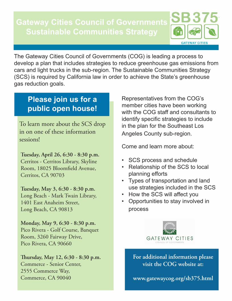
Representatives from the COG’s member cities have been working with the COG staff and consultants to identify specific strategies to include in the plan for the Southeast Los Angeles County sub-region.
Please join us for a public open house!
To learn more about the SCS drop in on one of these information sessions!
The Gateway Cities Council of Governments (COG) is leading a process to develop a plan that includes strategies to reduce greenhouse gas emissions from cars and light trucks in the sub-region. The Sustainable Communities Strategy (SCS) is required by California law in order to achieve the State’s greenhouse gas reduction goals.
For additional information please visit the COG website at:
www.gatewaycog.org/sb375.html
Tuesday, April 26, 6:30 - 8:30 p.m.Cerritos - Cerritos Library, Skyline Room, 18025 Bloomfield Avenue, Cerritos, CA 90703
Tuesday, May 3, 6:30 - 8:30 p.m.Long Beach - Mark Twain Library, 1401 East Anaheim Street, Long Beach, CA 90813
Monday, May 9, 6:30 - 8:30 p.m.Pico Rivera - Golf Course, Banquet Room, 3260 Fairway Drive, Pico Rivera, CA 90660
Thursday, May 12, 6:30 - 8:30 p.m.Commerce - Senior Center, 2555 Commerce Way, Commerce, CA 90040
Come and learn more about:
• SCS process and schedule• Relationship of the SCS to local
planning efforts• Types of transportation and land
use strategies included in the SCS• How the SCS will affect you• Opportunities to stay involved in
process
Gateway Cities Council of GovernmentsSustainable Communities Strategy

�������������� ������������������� ������������ �������������
����������������� ���������������������
��������������������������������������������������������������������������� ���������� ������������������������������������������ ���
��������������������������!��"��� �����#������!"#���������������� ���������� ���������������������������������������������������������$��%&��������������������������'�������()*���������������������$���������������+��� ���+���������, �������������������� ���������� �������������
-���� �������������+������ �,�������������������������������������������� ����������������������������������������������������������� �,����������������������������������������������������������������� ��������������!��������������������������!���������������� ���.������������������������������������������������������������/ ����"������� �������������)�����" )������������ ��������������"�����
�������� �����������
Whereas,
Whereas,
�� �������������������������������
�����"�� ����� ������ !��������0�����!����
�����
%&���������()*�
�!�
������������*����
�!���� "������� �������������)�����" )�

�������������� ������������������� ������������ �������������
!����"��#�����������
$��%���������������
1��(2����3���
1��)���������*�������4����
1�� ������*�������4����������
1��-������������������#�������3���
1��3�����4����
��� ��������� ��������
����������
�������������������������
�����������������������������
������������������������������������
��������������
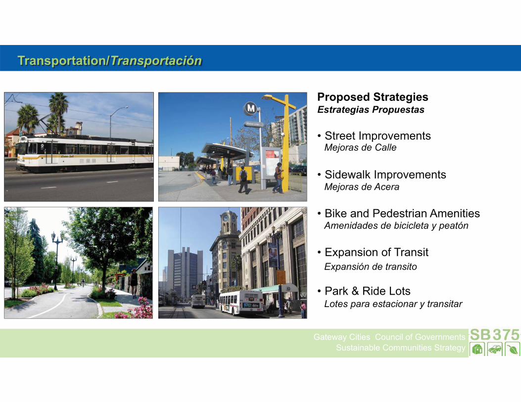
�������������� ������������������� ������������ �������������
&����%��������#� ����� ������
$��%���������������
1���������-�����������
1����������-�����������
1��#�������)���������!������
1��52���������� �����
1��)����6�"���7���
����������������
����������������
������������������������� ��!�
"� ����!�����������
#���� �����������������������
��� ��������� ��������
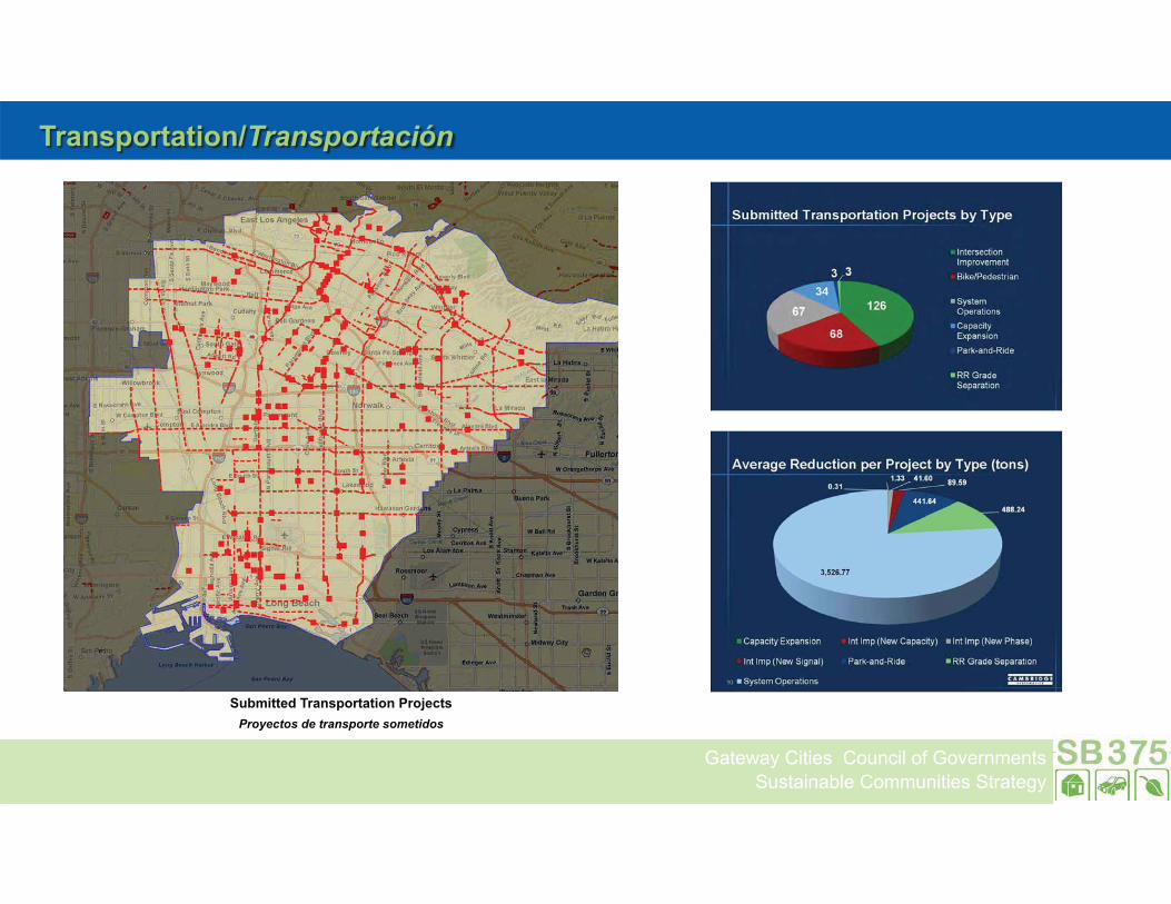
�������������� ������������������� ������������ �������������
&����%��������#� ����� ������
��������&����%���������$��'����� ������������ ����� ������������

�������������� ������������������� ������������ �������������
&����%���������(������)�����������&() #�������������������� ��� ����� ��
$��%��������������
1���� �����
1��# ��)����)������
1�� ������(�������
1��"���������)�������
���������$�
��� ��������� ��������
������������ �����������$�
����������%���!������������
��������� ������� ��������&����
'����� ������������&�(���������&�������� �����
"������������� ��)��������� ����&�(���������&�������� �����
��������� ������������&����������� ������1�5�������� ���"�� �����)������
1��)�����������)���������8�������
1�������������8�������7������!����

�������������� ������������������� ������������ �������������
&����%���������(������)�����������&() #�������������������� ��� ����� ��
$��%��������������
1������"� �������������
1�)��������� �� ���
1��#���-�������
��� ��������� ��������
*������������ ������������������������
"������������
��������������
�������������������������������
�����������������������������������������������
"������������� �������������
+������&��� �����������������������1�#����������
1��#��������������!��������
1��#���0�������4������
1��#���"����

�������������� ������������������� ������������ �������������
�*+���������������
,��-��� ����.���/�������
�#�9:;����������������������������������������������������<�� ����%+�=>>?��-������������������������������������������������ ���������� ������������������������������������������ ����� �������������/ ��������������������������������������������������������+�����, ��������� ����� �����������������������������������������������������.��������� ����������������������������������������������������������
�0+�������������1���2�����������31� ���������������*������@������������ ���������������������������� �������������������� ����������7���!�������� ����� ���*����������������������������������� ���������������� ��������� ��������.�����������+������������/ ����+������������� ���������+�������������������������������
��+��� ������������������ ������ �� ���� ������������ ������������������������������� ���������� ������������������������������������ �������� ���������������������������������-������������������������������� ������
�4+��� �����������������������������%��5��������#�9:;������������������������������ �����
��+��� ��������.�������������������6�����7�-���� �������������������������������������$��7����3���5�����������������������)����� ����������������������������������������������������������2��������� �����
�8+����������������������������������������������������������������� �����������������������1�5������������1 ���������
�����������������������������������/ �����������������!�������������!�+���������������������������������'������()*�+�����/ ����������������������������������������������������� ���������������������������� ������A� ������������ �������������B����������������������������������������-��������������������������������������������������+��!��� ��������������A���������������������������B�����+�������������+��� ��������������������� ��������������+����������������� ����+�����������/ ����������������������������������������������
��+�9�2�����������������:�������������������������������� ����������������������'��� ������������������������������������
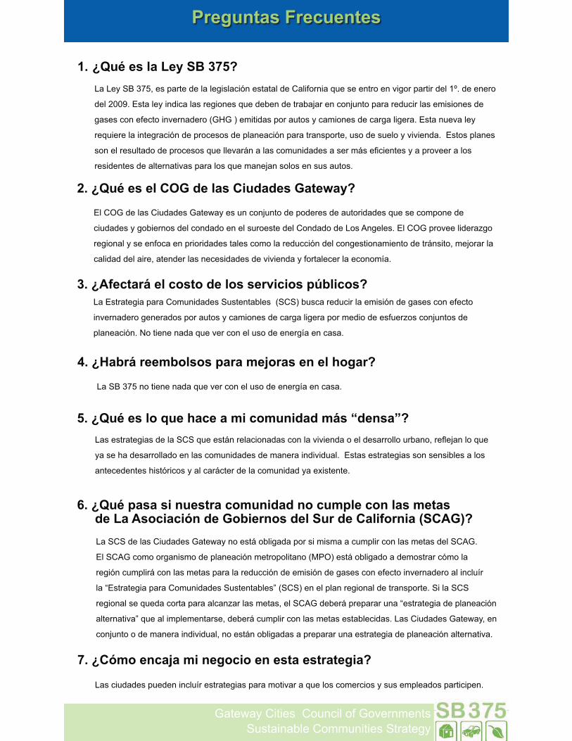
�������������� ������������������� ������������ �������������
�*+�;/<���� ��!���������
$��������,��������
7��7����#�9:;+�����������������������C���������������������/ �����������������������������%D�����������
����=>>?��5�������������������������/ ����������������@���������@ ������������ ������������������
����������������������������������������������� ������������������������������5����� ��������
��/ ��������������C������������������������C�����������������+� ������� ���������������5������������
���������� ������������������/ ��������E����������� ��������������E���.�������������������������
����������������������������������/ ������@������������� ��� ����
�0+�;/<����� ��31���� �����������1���2���
5��*��������� ����������������� �����@ ������������������� ���������/ ����������������
� ������������������������������������ ���������������������7���!��������5��*��������������'���
�������������������������������������������������� ��C���������������������������E����+���@��������
��������������+��������������������������������������������������������F��
��+�;�������=�� ���������� ������5������%>� �����7��5���������������� �������� ������������������ ������� ���������C����������������������
�������������������������� �������������������������������������������� ��'������@ ��������
�������C���G������������/ ������������� �����������F����������
�4+�;9���=������� ����%������'��������� �������
7���#�9:;��������������/ ������������� �����������F����������
��+�;/<���� ��-����������������������=��6�����7�7�����������������������/ �����E�������������������������������������������� �����+���H�@������/ ��
�������������������������������� ��������������������� �����5�����������������������������������
����������������C�������������E�������������� ���������2��������
�8+�;/<�%����������������������������% ������ ������������������!����������?�����1����������� �������� �����������1 �
7������������ ��������������������E����������������������� ������������������������!���
5���!��������������������������C����������������()*�����E����������������������C������
���C��� ����E�������������������������� ��C��������C��������������������������������������� F��
���A5���������������� �������� ����������B������������������������������������������������
�����������/ ��������������������'������������+�����!�������E���������� ���A��������������������C��
����������B�/ �����������������+������E�� ��������������������������������7��� �������������+����
���@ �������������������� ��+�������E���������������������� �����������������������C��������������
��+�;�?�������'��������������������������������
7���� ������� �������� F���������������������������/ ������������������ ����������������������
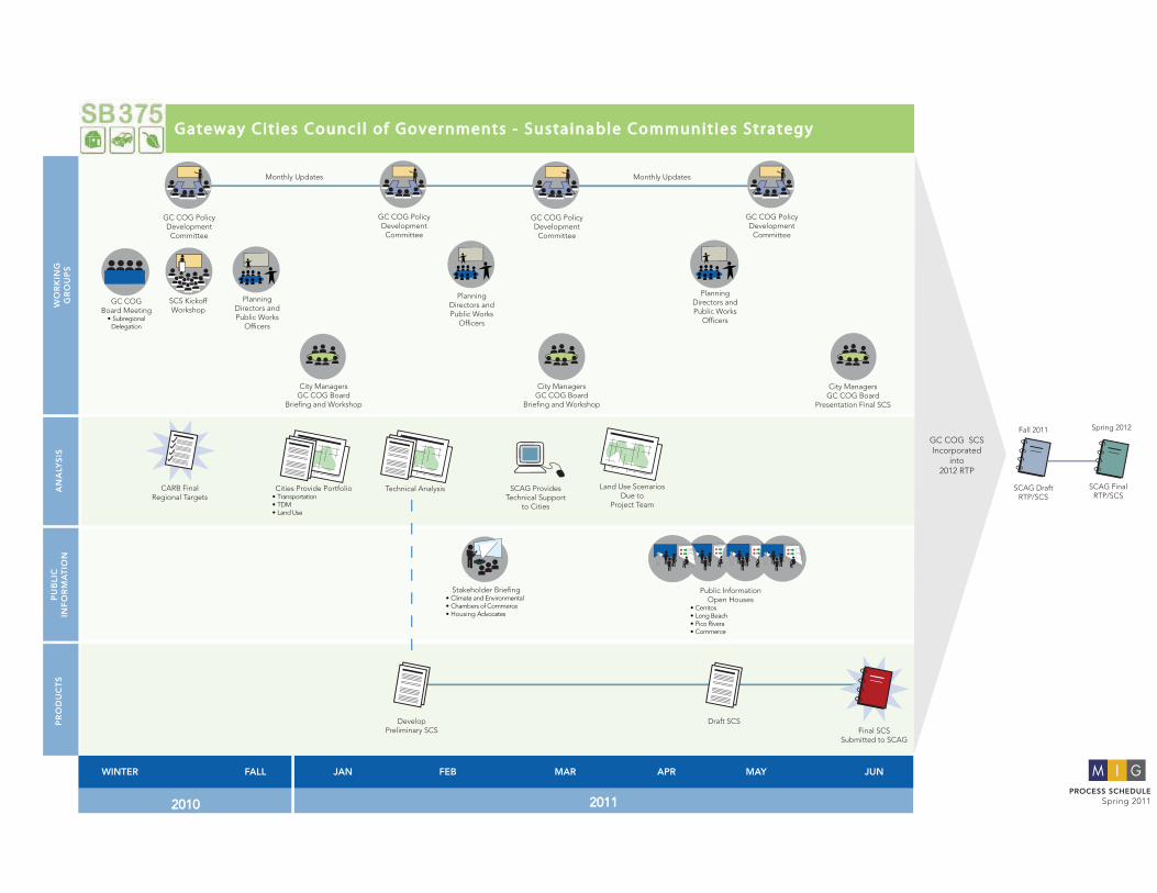
WO
RK
ING
G
RO
UP
S
WINTER FALL JAN FEB MAR APR MAY JUN
AN
ALY
SIS
PU
BLI
C
INF
OR
MA
TIO
N
GC COGBoard Meeting
Subregional Delegation
PROCESS SCHEDULESpring 20112010 2011
Cities Provide PortfolioTransportationTDMLand Use
Develop Preliminary SCS
Technical Analysis
PR
OD
UC
TS
SCS KickoffWorkshop
Planning Directors and Public Works
Officers
CARB Final Regional Targets
City ManagersGC COG Board
Briefing and Workshop
Planning Directors and Public Works
Officers
City ManagersGC COG Board
Presentation Final SCS
SCAG Provides Technical Support
to Cities
Land Use Scenarios Due to
Project Team
Stakeholder BriefingClimate and EnvironmentalChambers of Commerce
Advocates
Public Information
CerritosLong BeachPico RiveraCommerce
Draft SCSFinal SCS
Submitted to SCAG
GC COG SCSIncorporated
into2012 RTP
SCAG Draft RTP/SCS
SCAG Final RTP/SCS
Spring 2012Fall 2011
Gateway Cit ies Counci l of Governments - Sustainable Communit ies Strategy
City ManagersGC COG Board
Briefing and Workshop
Planning Directors and Public Works
Officers
GC COG Policy Development Committee
GC COG Policy Development Committee
Monthly Updates
GC COG Policy Development Committee
GC COG Policy Development Committee
Monthly Updates

GR
UP
OS
DE
TR
AB
AJO
INVIERNO OTOÑO ENE FEB MAR ABR MAY JUN
AN
ÁLI
SIS
INF
OR
MA
CIÓ
N A
L P
UB
LIC
O
Junta de la Mesa Directiva del GC COG
Delegación Subregional
CALENDARIOPrimavera 20112010 2011
Las Ciudades dan su CarteraTransporteTDMUso de Suelo
Desarrollo de la SCS Preliminar
Análisis Técnico
PR
OD
UC
TO
S
Taller de Lanzamiento
de la SCS
Directores de Planeación y Funcionarios
de Obras Públicas
CARB Final / Metas Regionales
Taller Informativo Administradores de las
Ciudades/Mesa Directiva de GC COG
El SCAG dá apoyo técnico a las
Ciudades
Fecha límite para los casos de uso de
suelo para el equipo de trabajo
Información a grupos interesadosClimáticos y ambientalesCámaras de Comercio
Información al PúblicoCerritosLong BeachPico RiveraCommerce
Borrador de la SCSVersión Final de la SCS presentada
al SCAG
GC COG SCS incorporada al
RTP 2012
Borrador SCAG
RTP/SCS
Versión Final RTP/SCS
Primavera 2012Otoño 2011
Consejo de Gobiernos de las Ciudades Gateway - Estrategia para Comunidades Sustentables
Comité de Desarrollo de Políticas de GC COG
Comité de Desarrollo de Políticas de GC COG
Actualizaciones Mensuales
Comité de Desarrollo de Políticas de GC COG
Comité de Desarrollo de Políticas de GC COG
Actualizaciones Mensuales
Directores de Planeación y Funcionarios
de Obras Públicas
Directores de Planeación y Funcionarios
de Obras Públicas
Taller Informativo Administradores de las
Ciudades/Mesa Directiva de GC COG
Taller Informativo Administradores de las
Ciudades/Mesa Directiva de GC COG
1
Gateway Cities COG SCS Overview
Spring 2011
Public Information
Open Houses

2
Background
Senate Bill 375 - Overview
• Legislation passed in 2008
• Aims at reducing greenhouse gas emissions (GHG) from cars and light trucks
• Includes mechanism for California Air Resources Board (CARB) to set GHG reduction targets for 2020 and 2035 to 1990 levels

3
Background
Senate Bill 375 - Approach
• Metropolitan Planning Organizations (MPOs) produce Sustainable Communities Strategy (SCS) as part of the Regional Transportation Plan (RTP)
• The Southern California Association of Governments (SCAG) - MPO for Southern California - will update its RTP by 2012

4
Background
Senate Bill 375 - Sustainable Communities Strategy (SCS)
• Is a regional GHG plan that links transportation, housing and land use to reduce GHG emissions from cars and light trucks
• Achieves GHG reduction targets set by the California Air Resources Board
5
Gateway Cities Sub-regional SCS
Gateway Cities Process
• Council of Governments (COG) have option to prepare SCS for sub-region
• Gateway Cities COG provides regional leadership for southeast Los Angeles County cities
• Gateway Cities COG Board chose SCS delegation in January 2010
• First effort of its type!

6
Gateway Cities Sub-regional SCS
Gateway Cities Approach
• Focus on three strategy categories for GHG Reduction
• Travel Demand Management • Land Use • Transportation projects
• Work with city staff to provide inputs
• Develop strategies consistent with cities’
plans

7
Process Schedule

8
Findings
Preliminary results indicate GHG reductions in Gateway sub-region meet the CARB regional targets
• Strategies contributing to reductions• Local transportation projects• Local land use projects• Travel Demand Management• Regional transportation projects

9
Lessons Learned
Some strategies result in greater reductions than others• Regional transportation projects• Local transportation projects
• Need to refine tools and models
• These lessons will assist in future 4-year planning cycles

10
Public Engagement
• Attend Public Information Open Houses• Cerritos• Long Beach• Pico Rivera• Commerce
• Attend Gateway Cities COG Board meeting• May – Draft SCS• June – Final SCS

11
Next Steps
• Final Gateway Cities SCS approval by Gateway Cities COG Board - June, 2011
• Submit Final Gateway Cities SCS to SCAG - June, 2011
• SCAG Incorporates Gateway Cities SCS into regional SCS and RTP - Summer 2011
• SCAG completes draft Regional SCS - Fall 2011
• SCAG submits final Regional SCS to CARB - Spring 2012

12
For additional information please visit the
COG website at:
www.gatewaycog.org/sb375.html

13
COG SCS CIUDADES GATEWAY
GENERALIDADES
Primavera 2011
Difusión Social
Juntas Informativas

14
Antecedentes
Ley del Senado 375 - Generalidades
• Se aprobó la legislación en 2008
• Trata de reducir la emisión de gases con efecto invernadero (GHG) producidos por autos y camiones de carga ligera
• Incluye mecanismos de la Junta de Recursos Atmosféricos de California (CARB) para establecer metas para la reducción de GHG en el 2020 y 2035 a los niveles de 1990
15
Antecedentes
Ley del Senado 375 - Enfoque
• Las Organizaciones Metropolitanas de Planeación (MPOs) diseñaron la Estrategia para Comunidades Sustentables (SCS) como parte del Plan Regional de Transporte (RTP)
• La Asociación de Gobiernos del Sur de California (SCAG)-MPO para el Sur de California, actualizará su RTP para el 2012

16
Antecedentes
Ley del Senado 375 – Estrategia para Comunidades Sustentables (SCS)
• Es un plan regional de GHG que relaciona el transporte, la vivienda y el uso de suelo para la reducción en la emisión de GHG producidos por autos y camiones de carga ligera
• Alcanza las metas de reducción de GHG establecidos por la Junta de Recursos Atmosféricos de California

17
La SCS Subregional, Ciudades Gateway
Proceso de las Ciudades Gateway
• El Consejo de Gobiernos (COG) tiene la opción de preparar la SCS para la sub-región
• El COG de las Ciudades Gateway provee liderazgo regional para las ciudades del sureste del Condado de Los Angeles
• La Mesa Directiva del COG de las Ciudades Gateway optó por la delegar la SCS en enero del 2010
• ¡Son los primeros trabajos de este tipo!

18
La SCS Subregional, Ciudades Gateway
Enfoque de las Ciudades Gateway
• Enfoque en tres categorias para estrategias de reducción de GHG
• Gestión para la Demanda del Transporte• Uso de Suelo• Proyectos para transporte
• Trabajar con el personal de la ciudad para la retroalimentación de información
• Desarrollar estrategias que sean consistentes con los planes de la ciudad

19
Calendario del Proceso
20
Resultados
Los resultados preliminares indican que la reducción de GHG en la sub-región Gateway, cumplirá con las metas regionales establecidas por CARB
• Estrategias que contribuyen a la reducción• Proyectos locales para el transporte• Proyectos locales para uso de suelo• Gestión de la demanda de transporte• Proyectos regionales de transporte

21
Lecciones Aprendidas
Algunas estrategias resultan en una mayor reducción que otras
• Proyectos regionales de transporte• Proyectos locales de transporte
• Se necesita afinar los modelos y herramientas
• Estas lecciones ayudarán a futuro en los ciclos de planeación de 4 años

22
Participación Pública
• Asistir a las Juntas Informativas Abiertas al Público• Cerritos• Long Beach• Pico Rivera• Commerce
• Asistir a las Juntas de la Mesa Directiva del COG de las Ciudades Gateway
• Mayo – Borrador de la SCS• Junio – Versión Final de la SCS

23
Pasos a seguir
• Aprobación de la versión final de la SCS de las Ciudades Gateway por la Mesa Directiva del COG de las Ciudades Gateway - Junio 2011
• Presentación de la versión final de la SCS de las Ciudades Gateway al SCAG Junio 2011
• El SCAG incorpora la SCS de las Ciudades Gateway en la SCS regional y el RTP - Verano 2011
• El SCAG finalizará el borrador de la SCS regional Otoño 2011
• El SCAG presenta la versión final de la SCS regional a la CARB – Primavera 2012

24
Para obtener información adicional por
favor visite el sitio Web de COG en:
www.gatewaycog.org/sb375.html

Appendix D. List of Transportation Improvement Projects in the Gateway Cities

Gateway Cities Submitted Roadway Capacity Projects
City Project Name Project Description Location
Length
of
Project
(miles)
Facility
Type
Area
Type
No. of
Lanes
(Pre‐
Project)
No. of
Lanes
(Post‐
Project)ADT
(weekday)
ADT (18.4%
growth in
VMT)
Bell Gardens Eastern Avenue Widening The Street was widened by 5 feet to create better flow of traffic Eastern Avenue from Muller to
Florence1.5
Primary
Arterial
Urban 4 6 14,351 16,992
Commerce Washington Blvd
Reconsttuction
Reconstruct pavement in concrete, add 1 lane, traffic signals,
landscape & hardscape improvements, ADA ramps, RxR crossing,
street lights, etc.
Washington Blvd from I‐5 Fwy to
westerly City limit (west of Arrowmill)
2 Primary
Arterial
CBD 2 3 26,788 31,717
Downey LAKEWOOD BLVD
IMPROVEMENT ‐ Phase 2
Minor widening to provide three continuous travel lanes,
additional turn lanes, wider lanes and larger turning radii to
decrease congestion and accommodate truck traffic. Rehab
pavement, construct curb, gutter, and sidewalk, block wall(s),
center landscaped medians, street and ornamental pedestrian
lighting systems. Upgrade to traffic signal at Gardendale St and
Lakewood Bl.
On Lakewood Bl between Dalen Street
and Gardendale Street
0.44 Primary
Arterial
Urban 2 3 26,233 31,060
Downey PARAMOUNT MEDIAN Construction of raised medians, installation of landscaping and
irrigation system, construction of stamped concrete paving,
installation of accent tree lighting fixtures, and replacement of
traffic striping and pavement markings. Added to this contract
was the installation of a midblock traffic signal in front of Fire
Station No. 3.
On Paramount Bl between Florence
Avenue and Lubec Street
0.27 Primary
Arterial
Urban 2 2 35,332 41,833
Downey LAKEWOOD BLVD
IMPROVEMENTS PHASE 3
Minor widening to provide three 12‐foot travel lanes, minor
widening of intersections, traffic signal system upgrades, drainage
improvements, reduction of cross‐slopes, pavement removal and
resurfacing, construction of curb, gutter and sidewalk, raised
medians with landscaping, parkways with landscaping, install
pedestrian and street lighting system.
On Lakewood Bl from Florence Ave to
Telegraph Road
1.01 Primary
Arterial
Urban 2 3 45,921 54,370
Downey LAKEWOOD BLVD IMPR
PHASE 3A 5TH TO
FLORENCE
Minor widening to provide three 12‐foot travel lanes, center LS
medians, installation of decorative street lighting, construction of
a recycled water main, resurfacing of existing asphalt concrete,
and repair of miscellaneous concrete.
On Lakewood Bl between Fifth St and
Florence Ave
0.64 Primary
Arterial
Urban 2 3 20,101 23,800
Downey IMPERIAL LANDSCAPED
MEDIAN
Construction of raised LS medians, sidewalk, curb ramps, street
trees, solar‐powered irrigation systems, striping and signage
modifications. Construct new midblock traffic signal at school at
La Reina Ave, upgrade to the traffic signal at the intersection of
Imperial Highway at Downey Avenue.
On Imperial Hwy between Paramount
Bl and Bellflower Bl
1.9 Primary
Arterial
Urban 3 3 29,512 34,942
Downey IMPERIAL MEDIAN, SAFETY
& REHAB IMPROV PH 2
Minor widening to provide 11‐foot travel lanes, minor widening at
intersections, construction of new raised landscaped median
islands, rehabilitation of the existing pavement, reclaimed water
irrigation system, traffic signal improvements and modifications,
sound walls, sidewalk, curb ramps, and signing and striping
modifications.
On Imperial Hwy between Old River
School Rd and Paramount Bl and
between Bellflower Bl and Woodruff
Avenue
1.44 Primary
Arterial
Urban 3 3 29,602 35,048

Gateway Cities Submitted Roadway Capacity Projects
City Project Name Project Description Location
Length
of
Project
(miles)
Facility
Type
Area
Type
No. of
Lanes
(Pre‐
Project)
No. of
Lanes
(Post‐
Project)ADT
(weekday)
ADT (18.4%
growth in
VMT)
Downey LAKEWOOD BLVD IMPR
FROM IMP HWY TO S & G
Constructing AC pavement; resurfacing with a variable AC overlay;
cold planning; curb and gutter, driveway approach; curb ramps
and sidewalk; local depressions and cross gutters; curb opening
catch basins; masonry walls; reclaimed water main and potable
water improvements; traffic signal upgrades, ornamental street
and pedestrian lights, irrigation and landscaping; and traffic
striping.
On Lakewood Bl from Imperial Hwy to
Stewart & Gray Rd
0.9 Primary
Arterial
Urban 2 3 23,112 27,364
Downey TELEGRAPH RD TRFIC
THRPUT & SFTY ENHCMTS
PHS 1
Construction of raised landscaped median islands On Telegraph Rd between the Passons
Bl and E City Limit
0.5 Primary
Arterial
Urban 2 3 48,039 56,879
La Mirada
Additional Lane on Artesia Restriping to add an additional lane Artesia from Knott and Valley View
1 Primary
Arterial
Urban 2 3 17,355 20,548
Long Beach Spring Street Transporation
Improvement Project
Roadway geometrics were modified to convert a 4 lane highway
into a six lane highway.
Spring Street between Cherry Avenue
and Redondo Avenue
Primary
Arterial
Urban 4 6 21,890 25,918
Long Beach Lakewood Bouevard
Transporation Improvement
Project
Parking was removed and roadway geometrics were modified to
convert this regional highway from 4 lanes to 6 lanes. Traffic
signals were modernized to facilitate traffic flow.
Lakewood Bouevard between Willow
Street and PCH.
Primary
Arterial
Urban 4 6 14,711 17,418
Long Beach PCH & Cherry Cities of Long Beach & Signal Hill are working collectively to
acquire property to widen Cherry Avenue to add a second travel
lane in Long Beach from the Signal Hill boarder to south of PCH.
Cherry Avenue between 19th Street
and 15th Street
Primary
Arterial
Urban 3.5 4.5 12,142 14,376
Norwalk Firestone Bridge Extend 3rd WB lane. Firestone Bridge over SG River 0.5 Primary
Arterial
Urban 2 3 61,490 72,804
Signal Hill 786 Cherry Ave Additional lanes 19th St to PCH 0.04 Primary
Arterial
Urban 2 4 17,882 21,172
Signal Hill 800 Crescent Heights Street
Improvement
Reconstruction of Crescent Street Cherry Ave to Gardena 0.1 Secondary Urban 2 4 8,899 10,536
Signal Hill California Avenue Reconstruction Patterson St to Willow Avenue 0.1 Secondary Urban 2 2 8,899 10,536
South Gate 424‐ST Kauffman and
Dorothy Ave Street
Widenings
Removal of existing improvement and widening on Kauffman Ave
and Dorothy Ave and construction and landscaping of median
island in Firestone Blvd
Kauffman and Dorothy Avenues
between Firestone Blvd and Southern
Ave
0.4 Secondary Urban 2 2 7,811 9,249
South Gate 409‐ST Willow Place
Widening
Removal of existing improvement and widening on Willow place Willow Pl between Santa Fe Ave and
Long Beach Blvd
0.3 Secondary Urban 2 2 7,811 9,249
South Gate I‐710/Rio Hondo Bridge
Widening Project
Widen both sides of Firestone Boulevard Bridge over the Rio
Hondo channel to provide a seven‐lane structure, three through
lanes in each direction with a median/turning lane.
Firestone Boulevard over Rio Hondo
Channel
0.2 Primary
Arterial
Urban 2 3 42,018 49,749
South Gate I‐710/Firestone Blvd
Interchange
This project involves widening south side of the Firestone
Boulevard Bridge over the Los Angles River to provide three
through lanes in each direction with a center raised median from
Rayo Ave to I‐710 freeway.
Firestone Boulevard over LA River 0.2 Primary
Arterial
Urban 2 3 58,662 69,455
Vernon 26th Street ‐ Widening &
Storm Drain
Widen 26th Street, added new C&G, shoulder, and middle lane.
Installation of storm drain system. New Traffic Signal System
Installation.
Project extended from 2500 feet west
of Indiana to west of Atlantic
Boulevard. New traffic signal on 26th
Street at Bonnie Beach Place (“T”
Intersection)
2.1 Secondary Urban 2 2.5 7,811 9,249

Gateway Cities Submitted Roadway Capacity Projects
City Project Name Project Description Location
Length
of
Project
(miles)
Facility
Type
Area
Type
No. of
Lanes
(Pre‐
Project)
No. of
Lanes
(Post‐
Project)ADT
(weekday)
ADT (18.4%
growth in
VMT)
Vernon Atlantic Blvd. Bridge over
the LA River
The City of Vernon proposes to widen Atlantic Blvd. bridge over
the Los Angeles River. Project will enhance the safety and
operational use of Atlantic Blvd. bridge over the Los Angeles River
and improve the intersection performance at District Blvd. The
project involves widening Atlantic Blvd. for approximately 1,300
linear feet to provide traffic shoulders, standard sidewalks and
extending the right‐turn lane over to the Atlantic Blvd. Bridge. The
proposed roadway configuration includes six 11‐foot through
traffic lanes, one northbound 11‐foot right turn lane, 4‐foot
minimum shoulders, 5' sidewalks, and a center median. The
adjacent intersection of Atlantic Blvd. and District Blvd. will be
reconfigured and the traffic timing optimized.
Project limits are from Atlantic Blvd.
north of the Los
Angeles River to 800 feet south of the
intersection with District Blvd. The
proposed project is located
approximately 0.25 miles (mi)
southwest of the Long Beach Freeway
(1‐710) in the City of Vernon.
Primary
Arterial
Urban 6 6.5 57,528 68,114

Gateway Cities Submitted Intersection Improvements ‐ New Signal
City Project Name Project Description Location Area Type
Facility
Type ‐
Total
Number
Facility
Type ‐
Total
Number of ADT ‐ Street 1 ADT ‐ Street 2
Peak Hour
Volume ‐ Street
Peak Hour
Volume ‐ Street
Proposed
Intersecti
Peak
Hour
Artesia Norwalk Blvd/186th St Replace obsolete signal controllers, install new
traffic signal, improve vehicle detection to reduce
traffic congestion
Norwalk Blvd/186th St Suburban Primary 4.5 Primary 4 12618 325 1262 33 60 50
Bell Gardens Signal at Fire Station 39 New Signal was installed at the Fire Station 39 to
facilitate movement of Fire Trucks in and out of
Station as as well as to be used by Pedestrian to
cross Garfield from City Hall to Post Office and
DMV across the Street
Garfield Avenue at Fire
Station 39
Suburban Primary 4.5 Secondary 1 24396 7645 2440 765 90 50
Cerritos Beach Street @
Carmenita Avenue,
Project No. 75072
New traffic signal Beach Street and Carmenita
Avenue
Suburban Secondary 2.5 Primary 5 7645 18076 765 1808 60 50
Cerritos Dumont Avenue @
Artesia Boulevard,
Project No. 45071
New traffic signal Dumont Avenue and Artesia
Boulevard
Suburban Primary 4.5 Secondary 1 20620 7645 2062 765 60 50
Commerce Garfield @ Slauson Reconstruct intersection in concrete, new traffic
signal, enhance turning radius, ADA ramps,
concrete repair (sidewalk, curb & gutter), etc.
Garfield & Slauson Suburban Primary 5 Primary 6 34173 21065 3417 2107 90 50
Commerce Telegraph @ Slauson Reconstruct intersection in concrete, new traffic
signal, enhance turning radius, ADA ramps,
concrete reparis (sidewalk, curb & gutter).
Telegraph & Slauson Urban Primary 6 Primary 6 41635 44326 4163 4433 90 50
Downey WOODRUFF/VIA
AMORITA TRAFFIC
SIGNAL
Installation of a new vehicle and pedestrian‐
actuated traffic signal, video detection, countdown
pedestrian signals, provide fiber optic
communication to the intersection to enable
remote traffic management and surveillance
Woodruff Ave, Via Amorita Suburban Primary 2 Secondary 1 7297 7645 730 765 60 50
Downey FLORENCE AVE /
ARRINGTON AVE
TRAFFIC SIGNAL
The installation of traffic signals at the intersection
of Florence Avenue and Arrington Avenue,
modifications to the traffic signals at the
intersection of Florence Avenue and Lakewood
Boulevard, and the purchasing of equipment
required for the application of thermoplastic
pavement markings to be installed.
Florence Ave, Lakewood Bl,
Arrington Ave
Urban Primary 7 Secondary 2 47055 7645 4706 765 60 50
Downey IMPERIAL
Improvements, La Reina
Ave
Construct new midblock traffic signal at school at
La Reina Ave
At Imperial Hwy and La
Reina Ave
Suburban Primary 7 Secondary 1 25863 16036 2586 1604 60 50
Long Beach Walnut Avenue
Transportation
Enhancement Project
Reconfigure two separate intersections into a
single intersection and provide new signalized
pedestrian crossings at a location that serves four
grade schools and adults accessing LBCC.
Walnut Avenue &
Alamitos/20th Street
Suburban Primary 2 Secondary 2 13615 7645 1362 765 60 50

Gateway Cities Submitted Intersection Improvements ‐ New Signal
City Project Name Project Description Location Area Type
Facility
Type ‐
Total
Number
Facility
Type ‐
Total
Number of ADT ‐ Street 1 ADT ‐ Street 2
Peak Hour
Volume ‐ Street
Peak Hour
Volume ‐ Street
Proposed
Intersecti
Peak
Hour
Long Beach LCD Traffic Enhancement
Project
Reconfigure the LCD (LOS COYOTES DIAGONAL) &
Studebaker Road/Parkcrest intersection into two
separate intersections to improve traffic opeations
and capacity while improving access to a new high
school currently underconstruction. Project also
includes reconfigeration of the lanes and traffic
signal operations at LCD & Carson Street to address
peak period congestion issues.
LCD (LOS COYOTES
DIAGONAL) between
Studebaker & Carson Street
Suburban Primary 4.5 Primary 6 27215 16292 2721 1629 60 50
Long Beach
Del Amo & Locust Intersec
Signalize intersection to provide improved
neighborhood connectivity and access to tranist
and park facilities
Del Amo Boulevard & Locust
Avenue
Suburban Primary 7 Secondary 2 37129 7645 3713 765 60 50
Long Beach
Park Avenue & Anahiem S
Installation of a new traffic signal to adress access
and traffic congestion related to Wilson High
School and events at Recreation Park.
Park Avenue & Anahiem
Street
Suburban Primary 2.5 Primary 5 25546 19562 2555 1956 60 50
Long Beach
2nd Street & Pomona Ave
Construction of a new traffic signal to facilitate
traffic flow during the peak period while also
providing a new signalized pedestrian crossing in a
dense retail shopping center.
2nd Street & Pomona
Avenue
CBD Primary 4.5 Secondary 1 25546 7645 2555 765 60 50
Maywood Slauson @ Loma Vista Traffic Signal Slauson @ Loma Vista urban Primary 5 Secondary 2 30740 2673 3074 267 60 50
Norwalk Project 7209 New traffic signal Rosecrans
Avenue/Greenstone Avenue
urban Primary 5.5 Secondary 2 49351 7645 4935 765 120 50
Norwalk Project 7219 New traffic signal Shoemaker
Avenue/Excelsior Drive
urban Primary 4 Secondary 2.5 16933 5050 1693 505 90 50
Norwalk Project 7214 New traffic signal Norwalk Boulevard/Cheshire
Street
Urban Primary 4 Secondary 2 14662 7645 1466 765 90 50
Norwalk Project 7215 New traffic signal Imperial Highway/Fairford
Avenue
Urban Primary 6.5 Secondary 2 56291 7645 5629 765 90 50
Norwalk Project 7211 New traffic signal Firestone
Boulevard/Paddison Avenue
Urban Primary 4.5 Secondary 2 28621 7645 2862 765 90 50
Paramount Downey and Madison Installation of new traffic signal Urban Primary 4.5 Secondary 2 15572 7645 1557 765 60 50
Paramount Orange and Jackson Installation of new traffic signal Urban Primary 4.5 Secondary 2 11804 619 1180 62 60 50
Paramount Somerset and El Camino Installation of new traffic signal Urban Primary 4.5 Secondary 2 15979 7645 1598 765 60 50
Paramount Garfield and Peterson Installation of new traffic signal Urban Primary 4.5 Secondary 2 35355 7645 3536 765 60 50
Paramount Garfield and Howery Installation of new traffic signal Urban Primary 4.5 Secondary 2 17623 7645 1762 765 60 50
Paramount Garfield and Exeter Installation of new traffic signal Urban Primary 4.5 Secondary 2 22934 7645 2293 765 60 50
Pico Rivera Beverly Boulevard
Median Rehabilitiaon
Project
Installation of new signalized intersection Beverly Boulevard and
Sandoval Avenue/Pico Park
Urban Primary 6.5 Secondary 2 65675 7645 6568 765 120 50

Gateway Cities Submitted Intersection Improvements ‐ New Signal
City Project Name Project Description Location Area Type
Facility
Type ‐
Total
Number
Facility
Type ‐
Total
Number of ADT ‐ Street 1 ADT ‐ Street 2
Peak Hour
Volume ‐ Street
Peak Hour
Volume ‐ Street
Proposed
Intersecti
Peak
Hour
Pico Rivera Traffic Signal Plan Installation of new signalized intersection Washington Boulevard and
Loch Alene Avenue
Urban Primary 6.5 Secondary 2 14409 535 1441 54 120 50
Pico Rivera Traffic Signal Plan Installation of new signalized intersection Rosemead Boulevard and
L.A. Fitness Driveway
Urban Primary 5 Secondary 2 28976 11721 2898 1172 120 50
SantaFe Springs Traffic signal; Norwalk at
Mora/Heritatge Springs
Drive
Installation of new traffic signal. Installation of right
turn only pocket for NB traffic
Norwalk Blvd. & Mora Dr. Suburban Primary 4.5 Secondary 2 19236 14289 1924 1429 60 50
SantaFe Springs Traffic signal; Bloomfield
at Heritage Springs Dr.
East
Installation of new traffic signal. Installation of right
turn only pocket for SB traffic.
Bloomfield & Heritage
Springs Dr. East
Suburban Primary 4.5 Secondary 2.5 16159 7645 1616 765 60 50
SantaFe Springs Traffic Signal; Florence at
Laurel (LA County)
Installation of new traffic signal at intersection of
Florence at Laurel
Florence Ave. & Laurel Ave. Urban Primary 4.5 Secondary 2.5 31564 7645 3156 765 60 50
SantaFe Springs Traffic Signal Installation
at Bloomfield at Corral
Installation of new traffic signal at intersection of
Bloomfield at Corral
Bloomfield Ave. & Corral Pl. Urban Primary 4.5 Secondary 2 24544 7645 2454 765 60 50
SantaFe Springs Traffic signal; Telegraph
at Villages Dr.
Installation of new traffic signal. Installation of
right turn only pocket for EB traffic
Telegraph Rd. & Villages
Drive, (new road between
Bloomfield and Norwalk)
Urban Primary 5.5 Primary 2 35845 7645 3584 765 60 50
Signal Hill 746 Traffic Signal Cherry
& 20th Street
New traffic signal (no signal or stop sign currently) Cherry Ave/ 20th St Suburban Primary 4.5 Secondary 2 17882 7645 1788 765 60 50
Signal Hill Orizaba & PCH Traffic
Signal
New traffic signal Orizaba & PCH intersection Urban Secondary 2 Primary 6.5 7645 54215 765 5421 60 50
South Gate 357‐TRF Traffic Signal at
Tweedy & Alameda
Installation/modification of traffic signals, lighting,
electrical systems, tree removals, and concrete
curb and sidewalk work.
Tweedy Blvd, Alameda St Urban Primary 4.5 Primary 6.5 13258 30990 1326 3099 60 50
Vernon New Traffic Signal 26th
at Bonnie Beach Pl
Widen 26th Street, added new C&G, shoulder, and
middle lane. Installation of storm drain system.
New Traffic Signal System Installation.
Project extended from 2500
feet west of Indiana to west
of Atlantic Boulevard. New
traffic signal on 26th Street
at Bonnie Beach Place (“T”
Intersection)
Suburban Secondary 2.5 Secondary 2.5 7645 7645 765 765 60 50

Gateway Cities Submitted Intersection Improvements ‐ New Signal
City Project Name Project Description Location Area Type
Facility
Type ‐
Total
Number
Facility
Type ‐
Total
Number of ADT ‐ Street 1 ADT ‐ Street 2
Peak Hour
Volume ‐ Street
Peak Hour
Volume ‐ Street
Proposed
Intersecti
Peak
Hour
Whittier Santa Gertrudes Avenue
at Starbuck Street
Installation of new traffic signal Santa Gertrudes Avenue and
Starbuck Street
Suburban Primary 4.5 Secondary 2.5 8703 7645 870 765 60 50
Whittier Philadelphia Street at
Whittier Greenway
Trail/Gregory Avenue
Installation of new traffic signal Philadelphia Street at
Whittier Greenway
Trail/Gregory Avenue
Urban Primary 4 Secondary 2 4539 7645 454 765 60 50
Whittier Pickering Avenue at
Bailey Street
Installation of new traffic signal Pickering Avenue at Bailey
Street
Suburban Secondary 2.5 Secondary 2 7645 7645 765 765 60 50
Whittier Hadley Street at Whittier
Avenue
Installation of new traffic signal Hadley Street at Whittier
Avenue
Urban Primary 4.5 Primary 4.5 16832 5993 1683 599 60 50

Gateway Cities Submitted Intersection Improvements ‐ New Phase
City Project Name Project Description Location
Intersection
Improvement Type
Type of
Turn with
New
Phase
Proposed
Intersection
Signal Cycle
Length (sec)
Number of
lanes for
which the
movement
is being
enabled
Cerritos Traffic Signal Modifications at 195th Street and
Norwalk Boulevard, Project No. 75041
Added left turn phasing 195th Street and Norwalk
Boulevard
Added left turn phasing Left 120 4
Cerritos Traffic Signal Modifications at Marquardt Avenue
and Artesia Boulevard, Project No. 75042
Added left turn phasing Marquardt Avenue and Artesia
Boulevard
Added left turn phasing Left 120 4
Cerritos Traffic Signal Modifications at 195th Street and
Pioneer Boulevard, Project No. 75044
Added left turn phasing 195th Street and Pioneer
Boulevard
Added left turn phasing Left 120 4
Cerritos Traffic Signal Modifications at 195th Street and
Studebaker Road, Project No. 75044
Added left turn phasing 195th Street and Studebaker
Road
Added left turn phasing Left 120 4
Downey PARAMOUNT/GALLATIN T.S. UPGRADE Traffic signal upgrades including E‐W left‐turn phasing,
implementation of vehicle video detection system, signal
communication system.
Paramount Bl. Gallatin Rd Improved phasing for left
or right turns only
Left 120 2
Downey PARAMOUNT/TELEGRAPH T.S. UPGRADE Traffic signal upgrades including E‐W left‐turn phasing,
implementation of vehicle video detection system, signal
communication system, emergency vehicle pre‐emption
system.
Paramount Bl, Telegraph Rd Improved phasing for left
or right turns only
Left 120 2
Downey WOODRUFF / WASHBURN TRAFFIC SIGNAL Upgrade of the existing traffic signal, including the installation
of accessible audible pedestrian devices to accommodate the
disabled
Woodruff Ave, Washburn Road Improved phasing for left
or right turns only
Left 90 4
Downey IMPERIAL HWY/COLUMBIA WY TRAFFIC SIGNAL Traffic signal upgrades, curb ramps. Imperial Hwy, Columbia Way Improved phasing for left
or right turns only
Left 90 4
La Mirada Alondra and Valley View Int. Improvement Extend westbound left turn lane Alondra and Valley View Signal phasing
improvement with LT
lanes
Left 90 1
Long Beach 7th Street & Park Avenue Reconfigure medians & add left‐turn phasing 7th Street & Park Avenue left 100 4
Long Beach Carson Street & Woodruff Avenue Intersection
Improvement Project
Modernize traffic signal control and provide improved left‐
turn phasing to improve safety and operations
Carson Street & Woodruff
Avenue
left 100 4
Long Beach Paramount & South Street Intersection
Enhancement Project
Modernize traffic signal to provide left‐turn phasing,
countdown pedestrain indications, and improved lighting to
address elevated accident rate and severe peak period
congestion
Paramount Boulevard & South
Street
left 100 4
Long Beach Atlantic Avenue & Carson Street Reconfigure travel lanes and install westbound left‐turn
arrows to improve safety and improve traffic operations
Atlantic Avenue & Carson
Street
left 100 1
Long Beach Spring Street & Woodruff Avenue Intersection
Improvement Project
Modernize traffic signal to provide left‐turn phasing in two
directions and improved pedestrian crossings to address
safety and congestion issues.
Spring Street & Woodruff
Avenue
left 100 2

Gateway Cities Submitted Intersection Improvements ‐ New Phase
City Project Name Project Description Location
Intersection
Improvement Type
Type of
Turn with
New
Phase
Proposed
Intersection
Signal Cycle
Length (sec)
Number of
lanes for
which the
movement
is being
enabled
Long Beach Willow Street & Woodruff Avenue Intersection
Improvement Project
Moderrnize traffic signal to provide left‐turn phasing and
improved pedestrian crossings to address congestion issues at
this intersection that provides access to and from the I‐405
freeway ramps
Willow Street & Woodruff
Avenue
left 100 4
Long Beach Magnolia & Willow Add Left‐turn phasing to improve access to freeway and
reduce congestion
Magnolia Avenue & Willow
Street
left 100 4
Long Beach Pine & Ocean Transporation Enhancement Project Modernization of an existing traffic signal to provide adaptive
control and left‐turn phasing to address congestion arrising
from brisk pedestrian and vehcile demand related to special
events and other evening activity.
Pine Avenue & Ocean
Boulevard
left 100 4
Long Beach Studebaker & Willow Intersection Improvement Project to modernize the traffic signal to provide left‐turn
phasing, countdown pedestrian indications, and modification
of landscaped medians to address congestion issues and
facilitate the safe and orderly movement of left‐turn vehicles.
Studebaker Road & Willow
Street.
left 100 4
Long Beach Studebaker Road & Wardlow Road Intersection
Improvement
Project to modernize the traffic signal to provide left‐turn
phasing, countdown pedestrian indications, and modification
of landscaped medians to address congestion issues and
facilitate the safe and orderly movement of left‐turn vehicles.
Studebaker Road & Wardlow
Road
left 100 4
Long Beach PCH & Cherry Caltrans modernized the traffic signal to provide adaptive
control and left‐turn phasing to address congestion issues.
PCH & Cherry Avenue left 100 4
Long Beach Bellflower Boulevard & Anahiem Road Traffic Signal
Upgrade
The signalized intersection was modernized and left‐turn
phasing was installed to improve traffic operations, reduce
congestion, and improve safety.
Bellflower Boulevard &
Anaheim Road
Left 100 4
Paramount Flower and Downey N/S bound protective Left turn phasing Left 90 2
Pico Rivera Beverly Boulevard Rehabilitaion Project Part of the improvements Is the signal modification at Beverly
Boulevard and Durfee Avenue
Beverly Boulevard and Durfee
Avanue
Improved phasing for left
or right turns only
Left 120 4
Signal Hill Willow & Walnut Traffic Signal Left‐turn phasing traffic signal Willow & Walnut intersection New signal or signal
phasing improvement
impacting all approaches
Left 90 4
Signal Hill Willow & Orange Traffic Signal Left‐turn phasing traffic signal Orange and Willow
intersection
New signal or signal
phasing improvement
impacting all approaches
Left 90 4
South Gate 343‐TRF Traffic Signal Upgrade at Tweedy Blvd and
Hildreth
Modify traffic signal and construct handicap access ramps Tweedy Blvd, Hildreth Ave New signal or signal
phasing improvement
impacting all approaches
Left 90 4
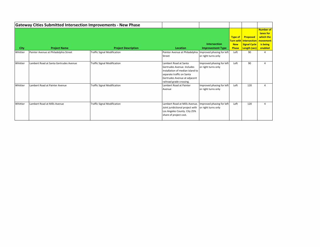
Gateway Cities Submitted Intersection Improvements ‐ New Phase
City Project Name Project Description Location
Intersection
Improvement Type
Type of
Turn with
New
Phase
Proposed
Intersection
Signal Cycle
Length (sec)
Number of
lanes for
which the
movement
is being
enabled
Whittier Painter Avenue at Philadelphia Street Traffic Signal Modification Painter Avenue at Philadelphia
Street
Improved phasing for left
or right turns only
Left 90 4
Whittier Lambert Road at Santa Gertrudes Avenue Traffic Signal Modification Lambert Road at Santa
Gertrudes Avenue. Includes
installation of median island to
separate traffic on Santa
Gertrudes Avenue at adjacent
railroad grade crossing.
Improved phasing for left
or right turns only
Left 90 4
Whittier Lambert Road at Painter Avenue Traffic Signal Modification Lambert Road at Painter
Avenue
Improved phasing for left
or right turns only
Left 120 4
Whittier Lambert Road at Mills Avenue Traffic Signal Modification Lambert Road at Mills Avenue.
Joint juridictional project with
Los Angeles County. City 25%
share of project cost.
Improved phasing for left
or right turns only
Left 120 4

Gateway Cities Submitted Intersection Improvements ‐ Capacity
City Project Name Project Description Location Area Type
Facility
Type ‐
Street 1
Existing
Number of
Lanes ‐
Street 1
Facility
Type ‐
Street 2
Existing
Number of
Lanes ‐
Street 2
Total Lanes
After Imp. ‐
Street 1
Total Lanes
After Imp. ‐
Street 2
ADT Volume ‐
Street 1
ADT Volume ‐
Street 2
Peak Hour
Volume ‐
Street 1
Peak Hour
Volume ‐
Street 2
Intersection
Existing Signal
Cycle Length
(sec)
Bell Gardens Truck Impacted Intersection The intersection is being re‐constructeded to provided
exclusive Left Turn Pockets in the Noth and South
Direction to alocate more time to the east/west direction
to create better flow of traffic in that direction.
Florence Avenue and
Jaboneria Street
Urban Primary 6.5 Secondary 2 6.5 2.5 46593 6456 4659 646 120
Bell Gardens Truck Impacted Intersection The intersection is being re‐constructeded to provided
exclusive Left Turn Pockets in the Noth and South
Direction to alocate more time to the east/west direction
to create better flow of traffic in that direction.
Florence Avenue and Ajax
Street
Urban Primary 6.5 Secondary 2 6.5 2.5 45777 7645 4578 765 120
Bellflower Clark/Flower Restriping to create left turn pockets for eastbound and
westbound Flower Street at 3‐phase (split phase)
signalized intersection
Clark Avenue at Flower
Street
Suburban Secondary 4 Primary 4 4 4.5 16925 2150 1693 215 90
Downey IMPERIAL Improvements,
Downey Ave
upgrade to the traffic signal at the intersection of Imperial
Highway at Downey Avenue.
At Imperial Hwy and
Downey Ave
Urban 33095 45133 3309 4513 120
Downey PARAMOUNT/FLORENCE
TRUCK IMP INST
Intersection widening at NW and SE corners, installation of
right‐turn only lanes in N‐S direction, signal modification,
relocation of existing street lighting, construction of new
curb ramps, incidental pavement striping, markings, and
signage.
Paramount Bl, Florence
Ave
Urban Primary 4.5 Primary 6.5 5 6.5 20844 25546 2084 2555 120
Downey LAKEWOOD/FIRESTONE
INTERSECTION
Widening at SW corner, providing one thru and one right‐
turn only lane in east bound direction, installation of
pedestrian safety lighting, decorative sw, bollards, curb
ramp, asphalt paving, parkway and median trees and LS,
irrigation system, potable water main, curb, gutter,
striping and pavement markings.
Firestone Bl, Lakewood Bl Urban 6 Primary 7 7.5 7 25863 16036 2586 1604 120
Downey BELLFLOWER/IMPERIAL
INTERSECTION IMP
Construction of double left‐turn pockets in the
northbound and southbound directions on Bellflower
Boulevard and right‐turn pockets in the southbound,
eastbound and northbound directions, the reconstruction
of all four curb returns to provide 50‐foot radii,
modification of the existing traffic signal and incidental
utility relocations and lane restriping
Bellflower Bl, Imperial
Hwy
Urban Primary 4.5 Primary 6.5 5.5 7 15340 22951 1534 2295 120
Downey PARAMOUNT BLVD AT
FIRESTONE BLVD
IMPRVMTS
Construction of a right‐turn pocket in the eastbound
direction, widening of all four curb returns to provide 50‐
foot radii, modification of the traffic signal, incidental
utility relocations, curb ramps, sw, AC pavement, striping,
and signage modifications
Paramount Bl, Firestone
Bl
Urban Primary 6 Primary 6.5 6 7 14202 38785 1420 3878 120
Lakewood Carwood West Add Right Turn Lane
Woodruff s/b @ Carson Urban Primary 6 Primary 6.5 6.5 6.5 20642 17238 2064 1724 120
Lakewood Douglas Park Add Right Turn Lane
Paramount n/b @ Carson Urban Primary 5 Primary 6.5 5.5 6.5 4662 33534 466 3353 120
Lakewood Douglas Park Add two Left turn Lanes Cover w/b @ Cherry Urban Secondary 2 Primary 6.5 2.5 6.5 7645 27281 765 2728 90
Lakewood Lakewood Collection Add Left and right Turn Lanes Clark @ Candlewood Urban Primary 4 Primary 4.5 5 4.5 10512 8846 1051 885 120
Lakewood Lakewood Collection Add Through only lane Candlewood @ Lakewood Urban Primary 4 Primary 7.5 4.5 7.5 17138 27170 1714 2717 120
Lakewood Lakewood Collection Add through and right turn lanes South St and Lakewood
Blvd
Urban Primary 4.5 Primary 6.5 6 6.5 16141 26320 1614 2632 120
Long Beach Redondo & Anahiem
Intersection Improvement
Widen Southbound Redondo Avenue to provide for right‐
turn lane
Redondo & Anaheim Urban Primary 4 Primary 4.5 4.5 4.5 18148 28084 1815 2808 90
Long Beach PCH & 2nd Street
Improvement Project
Widen Southbound PCH to provide for 2nd left‐turn lane
and right‐turn lane
PCH & 2nd Street Urban Primary 6 Primary 7 7.5 7 45505 47920 4551 4792 120
Long Beach PCH & Atlantic Avenue
Intersection Improvement
Widen Northbound Atlantic Avenue to provide for right‐
turn lane and traffic signal overlap phase
PCH & Atlantic Avenue Urban Primary 6.5 Primary 4.5 6.5 5 46648 8102 4665 810 120

Gateway Cities Submitted Intersection Improvements ‐ Capacity
City Project Name Project Description Location Area Type
Facility
Type ‐
Street 1
Existing
Number of
Lanes ‐
Street 1
Facility
Type ‐
Street 2
Existing
Number of
Lanes ‐
Street 2
Total Lanes
After Imp. ‐
Street 1
Total Lanes
After Imp. ‐
Street 2
ADT Volume ‐
Street 1
ADT Volume ‐
Street 2
Peak Hour
Volume ‐
Street 1
Peak Hour
Volume ‐
Street 2
Intersection
Existing Signal
Cycle Length
(sec)
Long Beach Los Alamitos Traffic Circle
Improvement Project
Cooperative Project with Caltrans to implement changes
to the traffic characteristics of the facility to improve
capacity and reduce accidents
PCH, Lakewood
Boulevard, LCD
Urban Primary Primary 48154 11196 4815 1120
Long Beach 2nd Street & Studebaker
Intersection Improvement
Project
Reconfigure intersection geometrics through the removal
of a median to add a third westbound travel lane
2nd Street & Studebaker
Road
Suburban Primary 5.5 Primary 5.5 6.5 5.5 39559 29293 3956 2929 90
Long Beach Wardlow Road & Cherry
Avenue Intersection
Improvement Project
Roadway geometrics were modified to provide a third
southbound through lane and a northbound right‐turn
lane. Traffic signal was modernized to provide adaptive
control to address varring traffic demands.
Wardlow Road & Cherry
Avenue
Urban Primary 4.5 Primary 5.5 5.5 5.5 2431 28873 243 2887 90
Long Beach Wardlow Road & Orange
Avenue Intersection
Improvement Project
Wardlow Road was widened to provide left‐turn pockets
and the trafic signal was modernized to provide left‐turn
phasing improving access to and from the freeway and
airport industrial areas.
Wardlow Road & Orange
Avenue
Urban Primary 4 Primary 4.5 4.5 4.5 9792 17622 979 1762 90
Norwalk McDonalds Install a WB right turn only lane. WB Imperial Highway at
Norwalk Boulevard
Urban Primary 6 Primary 7 6.5 7 56291 21959 5629 2196 120
Santa Fe Springs RTO for WB Telegraph at
SFS Rd.
Installation of right turn only pocket for WB traffic at the
intersection of Telegraph at Santa Fe Springs Rd
Telegraph Road & Santa
Fe Springs Rd.
Suburban Primary 6.5 Secondary 4.5 7 4.5 35845 13833 3584 1383 120
South Gate 303‐ST Firestone Blvd and
Garfield Ave Intersection
Improvements
Widen the west side of Garfield Ave, install right turn
lanes, construct PCC concrete pavement approaches on
three legs, asphalt pavement, modification of medians,
construction of catch basin and connector pipe, traffic
signal modifications, street light relocations, ADA ramps,
curb, gutter, sidwalk, and landscape restoration
Firestone Blvd, Garfield
Ave
Urban Primary 7.5 Primary 6 7.5 6.5 61950 39694 6195 3969 90
Vernon Atlantic Blvd. And District
Blvd Intersection
Improvement
The City of Vernon proposes to widen Atlantic Blvd. bridge
over the Los Angeles River. Project will enhance the safety
and operational use of Atlantic Blvd. bridge over the Los
Angeles River and improve the intersection performance
at District Blvd. The project involves widening Atlantic
Blvd. for approximately 1,300 linear feet to provide traffic
shoulders, standard sidewalks and extending the right‐turn
lane over to the Atlantic Blvd. Bridge. The proposed
roadway configuration includes six 11‐foot through traffic
lanes, one northbound 11‐foot right turn lane, 4‐foot
minimum shoulders, 5' sidewalks, and a center median.
The adjacent intersection of Atlantic Blvd. and District
Blvd. will be reconfigured and the traffic timing optimized.
Project limits are from
Atlantic Blvd. north of the
Los
Angeles River to 800 feet
south of the intersection
with District Blvd. The
proposed project is
located
approximately 0.25 miles
(mi) southwest of the
Long Beach Freeway (1‐
710) in the City of
Vernon.
Urban Primary 6.5 Primary 4.5 7 4.5 50661 26266 5066 2627 120

Gateway Cities Submitted System Operations/ Signal Sync / ITS
City Project Name Detailed Description Detailed Location
Length of
Project (mi)
Total # of
Lanes
# of
Signalized
Intersections
Affected
ADT
Volume
Peak hour
Traffic
Volume
Existing
Peak Hour
Travel Time
Existing
Average
Cycle Length
(secs)
Artesia Air Quaility Management
District
Traffic signal synchronization South Street 0.9 5 6 8848 885 3.5 100
Bellflower Artesia Blvd Signal synch City limit to City limit 2.6 5 8 10413 1,041 4.5 100
Bellflower Alondra Blvd Signal synch City limit to City limit 2.3 4.5 9 15295 1,530 4.5 100
Bellflower Bellflower Blvd Signal synch City limit to City limit 2.8 4.5 15 13727 1,373 6.0 100
Bellflower Boeing project mitigation Signal communication Bellflower portion: Bellflower Blvd:
SCL to 91 fwy
0.5 4.5 5 15922 1,592 1.5 100
Downey PARAMOUNT BLVD F.O.
SYSTEM, Phase I
Installation of fiber‐optic conduit/cable along
Paramount Bl, interconnection to existing signal comm
network at Telegraph, traffic signal upgrades, vehicle
video detection system
On Paramount Bl between
Telegraph Rd and Lubec St
1.0 5.5 6 24577 2,458 3.3 120
Downey FLORENCE AVENUE TRAFFIC
SIGNAL COMM SYS
Installation of fiber‐optic conduit/cable along the
length of Florence Ave, interconnection to existing
signal comm network at Lakewood Bl, traffic signal
upgrades, vehicle video detection, incidental utility
relocation, signage.
On Florence Ave between Old River
School Rd and the E City Limit
3.2 7 13 26763 2,676 6.8 100
Downey IMPERIAL HWY TRAFFIC
SIGNAL COMM SYSTEM
Installation of fiber‐optic conduit/cable along the
length of Imperial Hwy, interconnection to existing
signal comm network at Paramount Bl, Lakewood Bl,
traffic signal upgrades, vehicle video detection,
incidental utility relocation, signage.
On Imperial Hwy between Rives
Ave and Woodruff Ave
2.5 7 10 17903 1,790 4.9 120
Downey PARAMOUNT BLVD TRAFFIC
IMP‐FIRESTONE TO IMPERIAL
Installation of fiber‐optic conduit/cable along
Paramount Bl, traffic signal upgrades, coodinated
timing along corridor, comm network modifications at
TMC
On Paramount Bl between
Firestone Bl and Imperial Hwy
1.5 5.5 6 8807 881 3.2 120
Downey PARAMOUNT BLVD TRAFFIC
IMP‐FIRESTONE TO
FLORENCE
Installation of fiber‐optic conduit/cable along
Paramount Bl, traffic signal upgrades, coodinated
timing along corridor, comm network modifications at
TMC
On Paramount Bl between
Firestone Bl and Florence Ave
0.9 5.5 5 8224 822 1.8 120
Lakewood ATCS Cherry Ave/Del Amo to
Candlewood
LADOT's Adaptive Traffic Control System installed 0.5 6.5 2 15456 1,546 1.1 120
Lakewood ATCS Lakewood Blvd/Del
Amo to Ashworth
LADOT's Adaptive Traffic Control System installed 1.5 6.5 5 16105 1,610 3.0 100
Lakewood ATCS Bellflower Blvd/Del
Amo to Ashworth
LADOT's Adaptive Traffic Control System installed 1.5 6.5 4 11437 1,144 3.2 100
Lakewood ATCS Carson St/Paramount
to Lakewood Dr
LADOT's Adaptive Traffic Control System installed 1.0 7 5 21093 2,109 2.8 100
Lakewood ATCS Carson St/San Gabriel
River to Pioneer
LADOT's Adaptive Traffic Control System installed 0.7 7 4 31576 3,158 1.7 100
Lakewood ATCS Del Amo/Cherry Ave to
I‐605
LADOT's Adaptive Traffic Control System installed 4.4 6.5 11 16495 1,650 9.7 120
LAPW Alondra Blvd Traffic Signal
Synchronization Project
(TSSP)
Traffic Signal Syncronization improvements. Including
Providing additional vehicle detection to enable
operation of each signal as a fully traffic actuated
signal, and installing the appropriate components to
enable each signal to be capable of time‐based
coordination
Figueroa Street to La Mirada Bl 16.0 6 62 15295 1,530 29.1 100
LAPW Pacific /Long Beach Blvd
TSSP
Traffic Signal Syncronization improvements, additional
vehicle detection, traffic actuated signals, and time‐
based coordination.
Florence Av to Greenleaf Blvd 15.0 4 30 18243 1,824 27.0 90

Gateway Cities Submitted System Operations/ Signal Sync / ITS
City Project Name Detailed Description Detailed Location
Length of
Project (mi)
Total # of
Lanes
# of
Signalized
Intersections
Affected
ADT
Volume
Peak hour
Traffic
Volume
Existing
Peak Hour
Travel Time
Existing
Average
Cycle Length
(secs)
LAPW Bellflower Blvd TSSP See above. Lakewood Bl to PCH 7.0 6 47 13727 1,373 25.3 90
LAPW Eastern/Garfield/Cherry Av
TSSP
See above. Atlantic to PCH 15.0 4.5 61 13955 1,396 31.5 100
LAPW Artesia Bl TSSP See above. Alameda St to Valley View Av 11.0 6 34 10413 1,041 25.2 100
LAPW Central Av TSSP See above. El Segundo Bl to Victoria St 6.0 4.5 13 10720 1,072 14.0 100
LAPW Gage Av TSSP See above. Central Av to Slauson Av 8.0 4.5 40 11074 1,107 18.0 100
LAPW Whittier Av TSSP See above. Paramount Bl to Valley Home Av 9.0 4.5 34 21920 2,192 20.4 100
LAPW Wilmington Av TSSP See above. Imperial Hwy to Sepulveda Bl 6.0 4.5 37 11782 1,178 20.1 100
LAPW Carson St TSSP See above. Long Beach Bl to Bloomfield Av 7.3 6 28 17604 1,760 16.6 100
LAPW Bandini/37th St St/8th St
TSSP
See above. Alameda St to Garfield Ave 6.0 6 17 13445 1,345 14.6 100
LAPW Colima Rd/Lamirada Bl TSSP See above. Mar Vista Bl to Alondra Bl 5.5 6 19 17753 1,775 14.5 100
LAPW Garfield Av See above. Olympic Bl to Eastern Av 4.5 5 19 20731 2,073 13.4 100
LAPW Painter Av / Carmenita Rd
TSSP
See above. Hadley St to South St 9.0 4 30 12287 1,229 20.4 100
LAPW Studebaker Rd TSSP See above. Florence Av to Del Amo Bl 6.0 4.5 25 12256 1,226 15.8 100
LAPW Alameda St TSSP See above. Nadeau St to Auto Dr South 6.0 5 24 10425 1,043 21.2 100
LAPW Woodruff Av TSSP See above. Firestone Av to Willow St 9.0 5 26 10117 1,012 21.4 100
LAPW Leffingwell Rd TSSP See above. Imperial Hwy to Valley Home Av 4.5 5 14 16724 1,672 11.6 100
LAPW Beverly Bl TSSP See above. Pomona Bl to Pickering Av 7.5 5 34 20847 2,085 18.3 100
LAPW South St TSSP See above. Atlantic Bl to Studebaker Rd 5.0 5 13 9303 930 10.8 100
LAPW Washington Bl TSSP See above. Atlantic Av to Whittier Bl 8.0 6 29 24287 2,429 22.8 100
LAPW Lambert Rd TSSP See above. Washington Bl to Grayling Av 5.0 5 17 14445 1,444 11.8 100
LAPW I‐710/Atlantic Corridor ITS
Project
See above. Alameda St from Randolph Ave to
Industry Wy
4.5 4.5 13 18971 1,897 10.3 100
LAPW I‐5/Telegraph Corridor ITS
Project
Installation of fiber optic equipment and closed circuit
television cameras, the modification of traffic signals,
and the performance of other appurtenant work.
Telegraph Rd from Parmount Bl to
Carmenita Rd; Carmenita Rd from
Telegraph Rd to Imperial Hwy;
Bloomfield Ave from Telegraph Rd
to Emmens Wy; Emmens Wy from
Bloomfield Ave to Santa Fe Springs
Yard
4.6 7 20 48156 4,816 15.5 100

Gateway Cities Submitted System Operations/ Signal Sync / ITS
City Project Name Detailed Description Detailed Location
Length of
Project (mi)
Total # of
Lanes
# of
Signalized
Intersections
Affected
ADT
Volume
Peak hour
Traffic
Volume
Existing
Peak Hour
Travel Time
Existing
Average
Cycle Length
(secs)
LAPW I‐105 Corridor ITS Project See above. Firestone Bl from Stewart & Gray
Rd to Imperial Hwy; Imperial Hwy
from Firestone Bl to Carmenita Rd;
Imperial Hwy from Paramount Bl to
Bellflower Bl.
1.6 6.5 7 73006 7,301 3.6 100
LAPW I‐5 ATMS Integration Project See above. Imperial Hwy from Carmenita Rd to
Valley View Ave; Valley View Ave
from Imperial Hwy to Rosecrans
Ave
1.0 6.5 4 11782 1,178 2.5 100
Long Beach Ocean Boulevard
Transportation Enhancement
Project
Interconnect and modernize traffic signals along Ocean
Boulevard Corridor and add two new traffic signals to
improve safety and traffic operations
Ocean Boulevard between Alamitos
& Livingston/2nd Street
2.6 4 16 20069 2,007 7.2 100
Long Beach Atlantic Avenue
Transportation Enhancement
Project
Interconnect and modernize traffic signals along
Atlantic Avenue to improve operations and traffic
safety
Atlantic Avenue between Ocean
Boulevard & Wardlow Road
3.6 4 27 5593 559 9.0 100
Long Beach Studebaker Road ATCS and
Communictions
Enhancement Project
Construction of an eastside communications backbone
to support trafic signal control and motorist
information systems, conversion of traffic signal control
from fixed time to adaptive control.
Studebaker Road between Spring
Street and 2nd Street
3.6 4 12 13175 1,318 7.0 100
Long Beach Bellflower Boulevard Traffic
Signal Syncronization Project
Operational and timing improvements to traffic signals
along the Bellflower corridor throughout the City.
Bellflower Boulevard between 7th
Street & Del Amo Boulevard
5.0 6 20 349049 34,905 11.2 100
Long Beach Artesia Boulevard Traffic
Signal Syncronization Project
Operational and timing improvements to traffic signals
along the Artesia Boulevard corridor throughout the
City.
Artesia Boulevard between Long
Beach Boulevard and Downey Road
3.0 4 11 9144 914 6.5 100
Long Beach Wardlow Road Traffic Signal
Syncronization Project
Operational and timing improvements to traffic signals
along the Wardlow Road corridor in the western part of
the City.
Wardlow Road between Santa Fe &
the western City limit
0.5 4 3 18316 1,832 3.5 100
Long Beach Atlantic Avenue Cooridor
Improvement Project
Modernization of existing traffic signals, construction of
a new traffic signal, installation of left‐turn phasing,
installation of medians to reduce/eliminate vehicle
conflicts, along a retail corridor that is being renovated
to improve safety and faciliate traffic movement
Atlantic Avenue between 55th
Street & 61st Street
0.6 4 4 10162 1,016 2.0 100
Lynwood Long Beach Blvd.
Synchronization Project
Synchronization of 10 Traffic Signals in Lynwood. Part
of the County's synchronization progam.
Long Beach Blvd. from south city
limit to north city limit.
2.0 4 10 17534 1,753 4.0 100
Lynwood Atlantic Avenue
Synchronization Project
Synchronization of 10 Traffic Signals in Lynwood. Part
of the County's synchronization program which
includes the installation of KITS for the City.
Atlantic Avenue from south city
limit to north city limit
3.0 4 10 14736 1,474 6.0 100
Norwalk Project 7166 LA County TSSP Alondra Boulevard 1.5 4 4 15295 1,530 3.2 100
Norwalk Project 7155 LA County TSSP Studebaker Road 3.5 4 14 12256 1,226 7.0 100
Norwalk Project 7157 LA County TSSP Firestone Boulevard 1.0 5 4 21307 2,131 4.6 100
SantaFe Springs Painter‐Carmenita Rd. Signal
synchronization project (LA
County)
Painter/Carmenita Road 3.8 5 16 12287 1,229 6.0 105
SantaFe Springs I‐5/Telegraph Rd. ITS Project
(LA County)
I‐5/Telegraph Road 3.0 5 13 25032 2,503 5.0 105
Signal Hill 673 Orange Ave Signal
Upgrades
Replace traffic signals 32nd and 33rd Streets @ Orange
Ave
0.1 2 2 5085 509 0.9 100
Signal Hill Boeing ATCS Synchronize traffic signals Cherry Avenue corridor (Long Beach
and Signal Hill)
1.4 7 7 15456 1,546 3.4 100

Gateway Cities Submitted System Operations/ Signal Sync / ITS
City Project Name Detailed Description Detailed Location
Length of
Project (mi)
Total # of
Lanes
# of
Signalized
Intersections
Affected
ADT
Volume
Peak hour
Traffic
Volume
Existing
Peak Hour
Travel Time
Existing
Average
Cycle Length
(secs)
Signal Hill Orange Avenue Corridor
Traffic Signal Synchronization
Synchronize traffic signals Spring Street to Hill Street 1.0 3 5 4460 446 2.9 100
South Gate 355‐ST Otis Street
Rehabilitation
Remove and replace pavement, grind and overlay
asphalt rubber hot mix, make sidewalk, curb, and
gutter repairs, reconstruct new ADA ramps, convert
street lighting to LED, install signal interconnect
conduit between Firestone and Southern Ave, make
traffic signal upgrades
Otis St from North City Limit to
South City Limit
1.8 4 6 8602 860 4.2 100
South Gate 358‐ST Atlantic Avenue
Improvements
Roadway pavement rehabilitation with asphalt rubber
hot mix, construction landscaped median island ,
sidewalk, curb, and gutter repairs, reconstruction of
curb ramps to meet Americans with Disabilities Act
standards, signal interconnect between Tweedy
Boulevard and Michigan Avenue and traffic signal
upgrades, and peripheral improvements
Atlantic Avenue from Firestone
Boulevard to South City Limit
1.2 4.5 4 13718 1,372 2.6 100
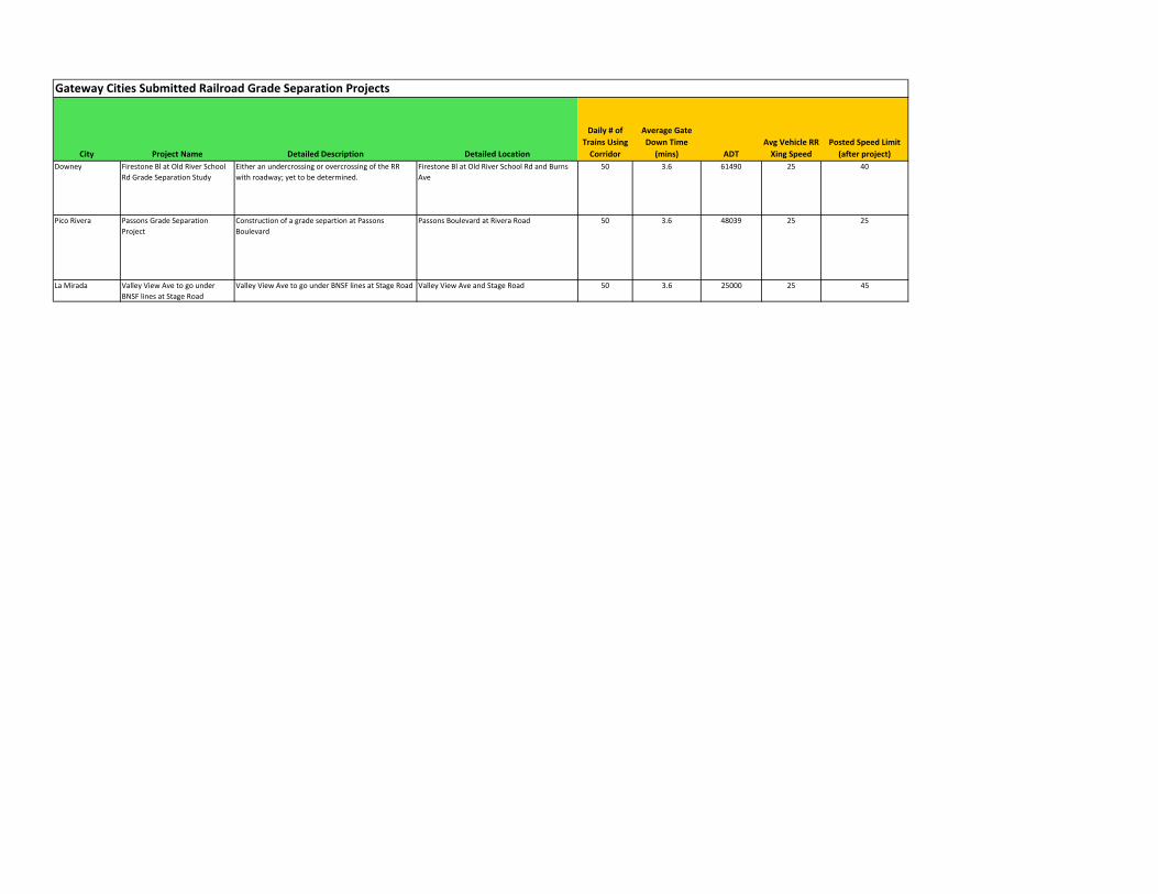
Gateway Cities Submitted Railroad Grade Separation Projects
City Project Name Detailed Description Detailed Location
Daily # of
Trains Using
Corridor
Average Gate
Down Time
(mins) ADT
Avg Vehicle RR
Xing Speed
Posted Speed Limit
(after project)
Downey Firestone Bl at Old River School
Rd Grade Separation Study
Either an undercrossing or overcrossing of the RR
with roadway; yet to be determined.
Firestone Bl at Old River School Rd and Burns
Ave
50 3.6 61490 25 40
Pico Rivera Passons Grade Separation
Project
Construction of a grade separtion at Passons
Boulevard
Passons Boulevard at Rivera Road 50 3.6 48039 25 25
La Mirada Valley View Ave to go under
BNSF lines at Stage Road
Valley View Ave to go under BNSF lines at Stage Road Valley View Ave and Stage Road 50 3.6 25000 25 45

Gateway Cities Submitted Non‐motorized Transportation Improvements (Bicycle/Pedestrian)
Location Project Name Detailed Description Detailed Location
Length of
Project (mi)
Bike, Ped
or Bike +
Ped?
Within 2 mi
of University
or College?
Access to
Transit?
Access to
Rail
Transit?
# of Activity
Centers within
1/2 mi of
project
# of Activity
Centers within
1/4 mi of project
Artesia American
Recovery and Re‐
Investment Act
Landscaped median,
sidewalk/handicapped ramp
improvements,street
pavement reconstruction
with recycled rubberized
asphalt
South Street 0.5 Bike + Ped N Y <3 <3
Artesia Safe Routes to
School Program
(State 5th Cycle)
Landscape Norwalk Blvd
frontage road and install
sidewalk for students
walking to school
Norwalk Blvd 0.1 Bike + Ped N Y N <3 <3
Bellflower West Branch
Greenway Multi‐
modal
Transportation
Corridor aka
Bellflower Bike
Trail
Class 1 bike and ped path Former PE ROW Lakewood
Blvd. to Caruthers Park
2.4 Bike + Ped Y Y N >6 >6
Downey PEDESTRIAN
IMPROVEMENTS ‐
FY05/06/07
(Blodgett)
Construct new sw, wc
ramps.
On Blodgett Ave from
Alameda St to Mory St; On
Mory St from Blodgett Ave
to Lakewood Bl; on Donovan
St between Birchdale
Avenue and Lakewood Bl;
8500 block of Orange St;
7700 block of Arnett St;
7700 block of Phlox St
0.9 Ped Only N N N <3 <3
Downey 3RD STREET
SIDEWALKS‐NEW
TO LA REINA
Construct tree wells, PCC,
install parkway trees
On Second, Third, and
Fourth St from New St to La
Reina Ave; on New St and La
Reina Ave from Firestone Bl
to Fourth St
0.62 Ped Only N Y N 4‐6 3
Downey SAFE ROUTE TO
SCHOOL‐OLD
RIVER SCHOOL
RD
Construct new sw, wc
ramps, modify traffic signal
at Old River School Rd at
Stewart & Gray Rd, remove
exist SCE street lighting
On Old River School Rd from
Laura St to Florence Ave
1.7 Ped Only N Y N 4‐6 3

Gateway Cities Submitted Non‐motorized Transportation Improvements (Bicycle/Pedestrian)
Location Project Name Detailed Description Detailed Location
Length of
Project (mi)
Bike, Ped
or Bike +
Ped?
Within 2 mi
of University
or College?
Access to
Transit?
Access to
Rail
Transit?
# of Activity
Centers within
1/2 mi of
project
# of Activity
Centers within
1/4 mi of project
La Mirada Beach Blvd Bike
Path
Path along flood control
channel
Hillsborough Dr to Imperial
highway
0.5 Bike Only Y Y N >6 >6
Lakewood Douglas Park Add Class I Bike Path north side of Cover from
Paramount 0.25 mile east to
City Limit
Bike Only Y Y N >6 >6
Lakewood Safe Routes to
School
Pedestrian improvements
constructed to facilitate
routes.
16 schools ‐ 275 miles of
safe routes
Ped Only N Y N >6 >6
Lakewood Douglas Park
Bike Path
Bike‐Ped north side of Cover from
Paramount 0.25 mile east to
City Limit
Long Beach 9th Street
Pedestrian
Enhancement
Project
Signalize two intersections
and provide an all‐way stop
at a third to provide
improved connectivity for
pedestrians and cyclists
traveling along 9th Street to
access schools, medical
faclities, park facilities, and
shopping.
9th Street between Pacific
Avenue and Long Beach
Boulevard
Long Beach Linberg Middle
School
Transporation
Enhancement
Project
Upgrade of school zone
traffic controls including the
installation of a new
pedestrian traffic signal to
provide enhanced access to
the campus
Market Street & Lewis
Avenue
Long Beach Market Street
Transporation
Enhancement
Project
Reconfigure the roadway to
provide improved pedestrian
facilities (widen sidewalks,
enhanced pedestrian
crossings) and access to key
destinations (post office,
transit stops, fire station,
schools, shopping) for
pedestrians, cylists, and
motorists.
Market Street between Long
Beach Boulevard and
Atlantic Avenue

Gateway Cities Submitted Non‐motorized Transportation Improvements (Bicycle/Pedestrian)
Location Project Name Detailed Description Detailed Location
Length of
Project (mi)
Bike, Ped
or Bike +
Ped?
Within 2 mi
of University
or College?
Access to
Transit?
Access to
Rail
Transit?
# of Activity
Centers within
1/2 mi of
project
# of Activity
Centers within
1/4 mi of project
Long Beach 4th Street &
Lime Avenue
Construction of a new traffic
signal to address traffic
congestion and pedestrian
access issues to schools and
transit stops
4th Street & Lime Avenue
Long Beach Santa Fe Avenue
& 20th Street
Installation of a new traffic
signal to provide primary
access to Cabrillo High
School, Admiral Kidd Park,
and transit stops
Santa Fe Avenue & 20th
Street
Long Beach Orange Avenue
Transportation
Improvement
Project
Traffic Calming project to
narrow the roadway via
striping to reduce vehicle
speeds along this residential
collector street and to add a
traffic signal midway to
improve neighborhood
connectivity and access to
transit stops.
Orange Avenue between
Wardlow Road & Bixby Road
Long Beach Long Beach
Boulevard & 51st
Street
Installation of a new traffic
signal at a newly constructed
elementry school to provide
a signalized pedestrian
crossing to connect the
campus to the residential
areas it serves.
Long Beach Boulevard &
51st Street
Long Beach Walnut Avenue
& 4th Street
Intersection
Improvement
Modernize the traffic signal
to provide enhanced
pedestrian access to bus
stops and relocation of
signal and electrical
equipment to improve
pedestrian access to bus
stops.
Walnut Avenue & 4th Street

Gateway Cities Submitted Non‐motorized Transportation Improvements (Bicycle/Pedestrian)
Location Project Name Detailed Description Detailed Location
Length of
Project (mi)
Bike, Ped
or Bike +
Ped?
Within 2 mi
of University
or College?
Access to
Transit?
Access to
Rail
Transit?
# of Activity
Centers within
1/2 mi of
project
# of Activity
Centers within
1/4 mi of project
Long Beach 3rd Street &
Lime Avenue
Intersection
Improvement
Construction of a new traffic
signal in downtown to
improve pedestrain access
to a nearby grocery market,
schools, and transit stops.
3rd Street & Lime Avenue
Long Beach Belmont Shore
Green Lane and
Sharrows
Installed green painted bike
lanes with sharrows on 2nd
Street in Belmont Shore
along with modified "Share
the Road" signs. The results
include a 29% increase in
bicycle usage, about 400
more cyclists over the 3‐day
count period, about the
same as the increase in the
number of cyclists riding on
the green lane.
2nd Street in Belmont Shore,
between Livingston Dr. and
Bay Shore Ave.
0 N >6 >6
Long Beach Bicycle Boxes Installed bike boxes on the
left‐hand turn lane to safely
guide cyclists into the green
shared lanes when heavy
traffic makes merging from
the striped bike lane to the
shared lane more
challenging.
Marina to 2nd Street and
2nd Street at Bayshore
Avenue
Long Beach Bicycle Lanes to
California State
University, Long
Beach
Implemented Class II bicycle
lanes as a safe passage for
cyclists to travel to the
campus from nearby
housing or from longer
distances with a connection
to the regional San Gabriel
River bike path.
East and West streets
adjacent to the campus on
Atherton Street and on 7th
Street.
Y
Long Beach Naples Road Diet Replaced one automobile
lane with a Class II bicycle
lane.
Eastbound on 2nd Street
between Bayshore Bridge
and Marina Drive
1.02 Y >6 >6
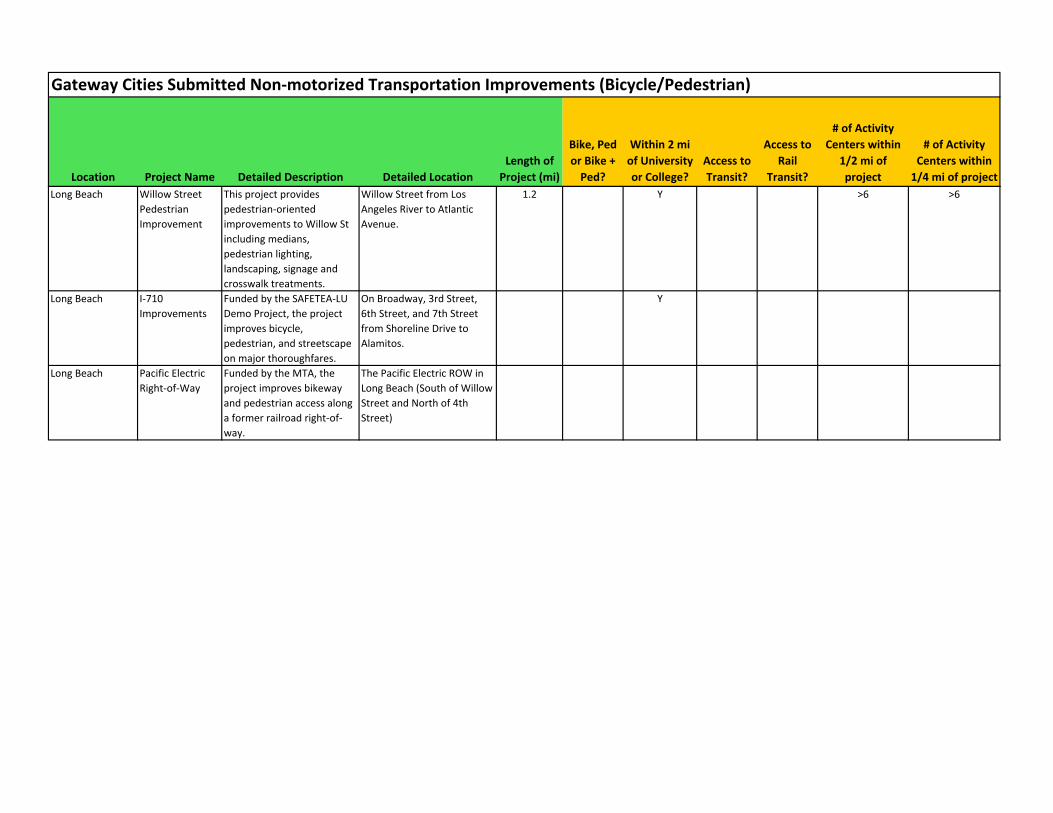
Gateway Cities Submitted Non‐motorized Transportation Improvements (Bicycle/Pedestrian)
Location Project Name Detailed Description Detailed Location
Length of
Project (mi)
Bike, Ped
or Bike +
Ped?
Within 2 mi
of University
or College?
Access to
Transit?
Access to
Rail
Transit?
# of Activity
Centers within
1/2 mi of
project
# of Activity
Centers within
1/4 mi of project
Long Beach Willow Street
Pedestrian
Improvement
This project provides
pedestrian‐oriented
improvements to Willow St
including medians,
pedestrian lighting,
landscaping, signage and
crosswalk treatments.
Willow Street from Los
Angeles River to Atlantic
Avenue.
1.2 Y >6 >6
Long Beach I‐710
Improvements
Funded by the SAFETEA‐LU
Demo Project, the project
improves bicycle,
pedestrian, and streetscape
on major thoroughfares.
On Broadway, 3rd Street,
6th Street, and 7th Street
from Shoreline Drive to
Alamitos.
Y
Long Beach Pacific Electric
Right‐of‐Way
Funded by the MTA, the
project improves bikeway
and pedestrian access along
a former railroad right‐of‐
way.
The Pacific Electric ROW in
Long Beach (South of Willow
Street and North of 4th
Street)

Gateway Cities Submitted Non‐motorized Transportation Improvements (Bicycle/Pedestrian)
Location Project Name Detailed Description Detailed Location
Length of
Project (mi)
Bike, Ped
or Bike +
Ped?
Within 2 mi
of University
or College?
Access to
Transit?
Access to
Rail
Transit?
# of Activity
Centers within
1/2 mi of
project
# of Activity
Centers within
1/4 mi of project
Long Beach South
Waterfront Bike
Path Connection
The South Waterfront Bike
Path Connection (SWBPC)
project is the construction of
a new Class I bike path
segment that closes an
existing gap in the area. The
project will include a mid‐
block crossing and
wayfinding. The SWBPC links
two primary segments of an
existing pathway system in
the south waterfront area to
one of Downtown Long
Beach’s primary pedestrian
and bikeway networks. This
proposed path closes a vital
gap between the existing
Class I path across
Queensway Bridge and the
existing Class I bike and
pedestrian path along the
south waterfront,
connecting the Greater
Downtown with the hotels
and commercial centers
located across the harbor.
This proposed bike path
creates a safe and much
needed segment that
connects two existing
systems and provides what
will be both an alternate
The proposed South
Waterfront Bike Path starts
at the north end of the
Queensway Bridge at the
existing terminus of the
Class I path. The proposed
alignment follows the north
side of Queensway Drive
within the City right‐of‐way
as a Class I bike path to the
Special Events Park existing
Class I path. Total proposed
bike path ditance in miles:
0.3.
0.3 N 4‐6 3

Gateway Cities Submitted Non‐motorized Transportation Improvements (Bicycle/Pedestrian)
Location Project Name Detailed Description Detailed Location
Length of
Project (mi)
Bike, Ped
or Bike +
Ped?
Within 2 mi
of University
or College?
Access to
Transit?
Access to
Rail
Transit?
# of Activity
Centers within
1/2 mi of
project
# of Activity
Centers within
1/4 mi of project
Long Beach 3rd Separated
Bikeway
Dedicated bike lanes on
Broadway and 3rd in
downtown Long Beach will
encourage residents,
families, and visitors to
participate in a more bike
friendly downtown. Initially,
the pilot will include a
painted island to separate
the bike lane. One traffic
lane will be lost to preserve
parking on both sides of the
street.
3rd from Alamitos and
Golden Avenue
1.16 Y >6 >6
Long Beach Broadway
Separated
Bikeway
See above Broadway from Alamitos
and Golden Avenue
1.15 Y >6 >6
Long Beach Third Street
Street Bike Lanes
Bike lanes (Class II) along
Third Street between
Alamitos/Junipero and Bike
lane on Third Street b/w
Alamitos/Junipero
Third Street between
Alamitos/Junipero
1 Y >6 >6

Gateway Cities Submitted Non‐motorized Transportation Improvements (Bicycle/Pedestrian)
Location Project Name Detailed Description Detailed Location
Length of
Project (mi)
Bike, Ped
or Bike +
Ped?
Within 2 mi
of University
or College?
Access to
Transit?
Access to
Rail
Transit?
# of Activity
Centers within
1/2 mi of
project
# of Activity
Centers within
1/4 mi of project
Long Beach Vista Bike
Boulevard
In an effort to provide
sustainable transportation
alternatives to the
community, as well as a safe
route to several
neighborhood schools, the
City of Long Beach is
installing a “bike boulevard”
on Vista Street, extending
from Temple Avenue to
Nieto Avenue. The bike
boulevard on Vista Street
will provide a safe route to
school for students at Lowell
Elementary and Rogers
Middle School on the east,
and Horace Mann
Elementary on the west end
of Vista Street. More
broadly, the bike boulevard
will provide a convenient,
direct cycling option for
families with young children,
students, commuters, and
recreational cyclists.
Vista Street, from Temple
Ave to Nieto Ave
1.5 N >6 >6
Long Beach Daisy Street ‐
Bike Boulevard
Bike boulevard will provide
North‐South Class III bicycle
facility (running the length of
the City‐ from downtown to
70th).
running the length of the
City‐ from downtown to
70th
8.73 Y >6 >6
Long Beach Sixth Street ‐
Bike Boulevard
Bike boulevard will provide
East‐West Class III bicycle
facility (running from
Junipero to Park).
6th St from Junipero to Park 1.53 Y >6 >6

Gateway Cities Submitted Non‐motorized Transportation Improvements (Bicycle/Pedestrian)
Location Project Name Detailed Description Detailed Location
Length of
Project (mi)
Bike, Ped
or Bike +
Ped?
Within 2 mi
of University
or College?
Access to
Transit?
Access to
Rail
Transit?
# of Activity
Centers within
1/2 mi of
project
# of Activity
Centers within
1/4 mi of project
Long Beach Long Beach Blvd.
Pedestrian
Improvement
Project
Project provides pedestrian‐
oriented improvements to
Long Beach Boulevard
including pedestrian lighting,
street trees, and crosswalk
treatments.
Long Beach Blvd b/t Willow
Ave & I‐405
0 Y >6 >6
Long Beach Atherton Street
Enhancement
Project
Rehabilitating the
landscaped median to
enhance the experience of
over 37,000 pedestrians,
bicyclists, transit users and
autos daily.
Bellflower & Los Cerritos
Channel
Long Beach Willow Street
Pedestrian
Improvement
Project
This project provides
pedestrian‐oriented
improvements to Willow St
including medians,
pedestrian lighting,
landscaping, signage and
crosswalk treatments.
Willow St B/t LA River &
Atlantic
Long Beach San Gabriel River
Bike Path Closure
at Willow Street
Creation of off‐street bicycle
path to achieve bicycle route
gap closure on Willow Street
from the San Gabriel River
Bike Path west to
Studebaker Road
Willow St, at San Gabriel
River & Studebaker
0 Y <3 <3
Long Beach Carson Street
Bike
Improvement
Project
Add Bike Lanes on Carson
Street between Atlantic &
Long Beach Boulevard
Carson Street between
Atlantic & Long Beach
Boulevard
0 N >6 >6
Long Beach Atlantic Avenue
Bike Lane Project
Provide new bike lanes
connecting facilities on San
Antonio and those on Del
Amo
Atlantic Avenue north of
Bixby Knolls
0 N >6 >6
Long Beach Harding Street
Traffic Calming
Project
Reconfigure roadway
stripping to install bike lanes
and new pedestrian
crossings
Harding Street between
Atlantic Avenue and Cherry
Avenue
0 Y >6 >6

Gateway Cities Submitted Non‐motorized Transportation Improvements (Bicycle/Pedestrian)
Location Project Name Detailed Description Detailed Location
Length of
Project (mi)
Bike, Ped
or Bike +
Ped?
Within 2 mi
of University
or College?
Access to
Transit?
Access to
Rail
Transit?
# of Activity
Centers within
1/2 mi of
project
# of Activity
Centers within
1/4 mi of project
Lynwood Abbott Road
Improvement
Project
Roadway improvement
project that includes
upgrading existing sidewalk
and new sidewalk and curb
ramp installation.
Abbott Road (Martin Luther
King Jr. Blvd. to East City
Limit)
1.46 Ped Only N Y N >6 >6
Lynwood Sidewalk
Improvement
Project FY 09‐10
Reconstructed damaged
sidewalk and install new
sidewalk.
Various locations City Wide
(Major work Martin Luther
King Jr Blvd. and Clark
Avenue)
0.25 Ped Only Y Y N >6 >6
Lynwood Annual Sidewalk
Improvement
Project FY 10‐11
Reconstructed damaged
sidewalk and install new
sidewalk.
Various locations citywide. Ped Only N Y N <3 <3

Gateway Cities Submitted Non‐motorized Transportation Improvements (Bicycle/Pedestrian)
Location Project Name Detailed Description Detailed Location
Length of
Project (mi)
Bike, Ped
or Bike +
Ped?
Within 2 mi
of University
or College?
Access to
Transit?
Access to
Rail
Transit?
# of Activity
Centers within
1/2 mi of
project
# of Activity
Centers within
1/4 mi of project
Norwalk Norwalk/Santa
Fe
SpringsTransport
ation Center‐
Metrolink Park
and Ride ‐
Pedestrian Plaza
Upgrade
Upgrade of existing
passenger amenities for the
Pedestrian Plaza at the
regional inter‐modal
Norwalk/Santa Fe Springs ‐
Metrolink Transportation
Center. The projec includes
construction of a pedestrian
plaza with pathways for
bicycles and pedestrians, a
passenger car pick‐up/drop‐
off area to encourage access
to the buses and trains as
alternative modes of
transportation, seating
areas,security lighting,
signage, electronic bus
schedule information,
decorative paving and
landscaping. The project also
includes widening of the
approach into the
Transportation Center and
modifications to the
entrance to improve access
and visibility, as well as
signage improvements to
the transit center, bus
layover areas and park and
ride lot. The project is
intended to improve
pedestrian and vehicular
The project is located at the
Norwalk‐Santa Fe
SpringsIMetrolink
Transportation Centerand
Park and Ride at 12700
E.lmperial Highway,
Norwalk, CA 90650. The
transportation center serves
all of Los Angeles, Orange
and San Bernardino
Counties. This project is
totally enclosed within the
Norwalk/Santa Fe Springs
Transportation Center ‐
Metrolink Park and Ride.
< 1 Bike + Ped N Y Y 4‐6 <3

Gateway Cities Submitted Non‐motorized Transportation Improvements (Bicycle/Pedestrian)
Location Project Name Detailed Description Detailed Location
Length of
Project (mi)
Bike, Ped
or Bike +
Ped?
Within 2 mi
of University
or College?
Access to
Transit?
Access to
Rail
Transit?
# of Activity
Centers within
1/2 mi of
project
# of Activity
Centers within
1/4 mi of project
Pico Rivera Safe Route to
School Program
New sidewalk Loch Alene Avenue Balfour
Street, Catherne Street,
Lidsey Avenue, Havenwood
Drive, Kilgarry Aveneu,
Lemoran Avenue, Reichling
Lane, Coffman Pico Road,
Crossway Drive, Shade Lane,
Sideview Drive, Sunglow
Street, Roma Street,
Clarinda Avenue
2.5 Ped Only N Y N >6 >6
Pico Rivera CDBG‐R Sidewalk
Curb and Gutter
Improvemtents
Sidewalk Curb and Gutter
Improvemtents
Loch Alene Avenue 0.25 Ped Only N Y N <3 <3
SantaFe Springs Sorensen Avenue
Sidewalk
Improvements
Sorensen Avenue Bike + Ped N Y N <3 <3
SantaFe Springs New Bike Lanes
and Bike Lockers
Bike lanes connecting
Coyote Creek to Metrolink
Transportation Center and
to San Gabriel River Path;
and Bike lockers (total of 20
bike lockers) at Metrolink
station
Foster Rd. to Carmenita Rd.
to Orden Dr. west,
Leffingwell Rd. north, to
Adler Dr. west, to
Shoemaker Av. north, to
Imperial Hwy. west, to
Transit Center, then to
Bloomfield Ave. north, to Los
Nietos Rd. west, to the San
6 Bike Only Y Y Y >6 >6
Signal Hill 674 Coronado
Sidewalk
new sidewalk PCH and Coronado 0.02 Ped Only Y Y N >6 >6
Signal Hill 743 Illuminated
Crosswalk 19th
& Cherry
Crosswalk upgrade 19th St and Cherry Ave 0.01 Ped Only Y Y N >6 >6
Signal Hill 629 Willow
Street ADA
Improvements
ADA Ramps, new sidewalk Willow Street, between
California and Orange
0.1 Ped Only Y Y N >6 >6
Signal Hill 675 21st Street &
Stanley Sidewalk
new sidewalk Stanley and 21st Street 0.01 Ped Only Y N N <3 <3

Gateway Cities Submitted Non‐motorized Transportation Improvements (Bicycle/Pedestrian)
Location Project Name Detailed Description Detailed Location
Length of
Project (mi)
Bike, Ped
or Bike +
Ped?
Within 2 mi
of University
or College?
Access to
Transit?
Access to
Rail
Transit?
# of Activity
Centers within
1/2 mi of
project
# of Activity
Centers within
1/4 mi of project
Signal Hill 602 ADA Access
Improvements
Sidewalk improvements Orange and Willow 0.01 Ped Only Y Y N >6 >6
Signal Hill 606 Las Brisas St ‐
Phase 2
Sidewalk improvements California Ave Las Brisas area 0.02 Ped Only Y Y N >6 >6
Signal Hill Crescent Heights
Street Sidewalk
Improvements
Sidewalk improvements Gardena Street to Cherry
Ave
0.01 Ped Only Y Y N >6 >6
Signal Hill Citywide ADA
Sidewalk
Improvements
Sidewalk improvements Citywide 1 Ped Only Y Y N >6 >6
Signal Hill 612 25th Street
Improvement
Resurface street & construct
sidewalks, ADA ramps,
curb&gutter etc
Between Lewis and Orange
Avenues
0.2 Bike + Ped
South Gate Safe Route to
Schools Cycle 1
Construct a traffic signal,
countdown pedestrian
signals, flashing beacons/in‐
pavement crosswalk light,
install speed awareness
signs, and widen the
sidewalk adjacent to a new
school location
Pinehurst Ave between
Tweedy and Southern
0.5 Ped Only N N N 4‐6 4‐6
South Gate Safe Route to
Schools Cycle 2
Hold two educational
community workshops to
the benefits of
walking/biking, hiring a
coordinating consultant,
developing site specific
education materials, and
conducting education and
encouragement campaigns
Near 16 Primary schools
within South gate
Ped Only Y Y N >6 >6

Gateway Cities Submitted Non‐motorized Transportation Improvements (Bicycle/Pedestrian)
Location Project Name Detailed Description Detailed Location
Length of
Project (mi)
Bike, Ped
or Bike +
Ped?
Within 2 mi
of University
or College?
Access to
Transit?
Access to
Rail
Transit?
# of Activity
Centers within
1/2 mi of
project
# of Activity
Centers within
1/4 mi of project
South Gate Safe Route to
Schools Cycle 8
Construct 1.5 mi. Class I bike
path along Southern Ave and
2000 ft. sidewalk along
Tweedy Boulevard, install 98
ped heads, 17 driver speed
awareness signs, 6 speed
humps, 1 new flashing
beacon/in‐pavement light
system
Various locations near 14
schools. Bike path on
Southern Ave. between
State St and Burke Ave;
Sidewalk on Tweedy Blvd
from Pinehurst Ave to
Hildreth Ave
1.5 Bike + Ped Y Y N >6 >6
South Gate Safe Route to
Schools Cycle 9
Construct 1.2 miles of Class
II bike lanes and 1,500 feet
of raised center traffic
calming medians with
related encouragement
activities
Alexander Ave between
Firestone Blvd and Abbot Rd
(bike lane); and Southern
Ave between Vossler Ave
and Pinehurst Ave (medians)
1.2 Bike + Ped N N N <3 <3
South Gate Los Angeles River
Trail Head
Improvements
Make improvements on
existing facilities at two
locations along the Los
Angeles River Bicycle Trail.
At Hollydale Park existing
restroom facilities and
landscaping and at Southern
Avenue improvements to
the existing Los Angeles
River Bicycle Trail entrance.
Los Angeles River Trail Heads
located at Southern Ave
(east end) and Hollydale
Park.
Bike + Ped N N N <3 <3
Whittier Whittier
Greenway Trail
Class I Bike and Pedestrian
trail
Along abandon UPRR ROW
from Pioneer Blvd. to Mills
Ave.
5.2 Bike + Ped Y Y N >6 >6

Gateway Cities Submitted Non‐motorized Transportation Improvements (Bicycle/Pedestrian)
Location Project Name Detailed Description Detailed Location
Length of
Project (mi)
Bike, Ped
or Bike +
Ped?
Within 2 mi
of University
or College?
Access to
Transit?
Access to
Rail
Transit?
# of Activity
Centers within
1/2 mi of
project
# of Activity
Centers within
1/4 mi of project
Whittier Pio Pico Bikeway
Connection
Bikeway connection from
San Gabriel River Bike Path
to the Pio Pico State
Histrocial Park
Adjacent to Whittier
Boulevard from San Gabriel
River Bike Path to Pio Pico
State Historical Park
0.4 Bike + Ped N Y N <3 3
Whittier Greenleaf
Avenue Class II
Bike Lanes
Installation of Class II Bike
Lanes and Two‐Way Left‐
Turn Lane. Road Diet from 4
lane to 2 lane.
La Cuarta Street to South of
Mulberry Drive
1 Bike Only Y Y N >6 >6
Whittier Pioneer Blvd.
Class II Bike Lane
Installation of Class II
Northbound Bike Lane and
Southbound Sharrow Lane
on Pioneer Blvd. from
Whittier Greenway Trail to
Beverly Blvd.
Pioneer Blvd. from Whittier
Greenway Trail to Beverly
Blvd.
0.38 Bike Only N Y N <3 <3
Whittier Philadelphia
Street Class II
Bike Lanes
Installation of Class II Bike
Lanes adjactent to Whittier
College
Philadelphia Street from
Painter Avenue to Bryn
Mawr Way
0.25 Bike Only Y Y N >6 >6
Whittier Beverly
Boulevard Class II
Bike Lanes
Installation of Class II Bike
Lanes, Median Islands,
Safety Lighting and Bus
Shelters
Beverly Blvd. from 605
Freeway to Norwalk
Blvd./Workman Mill Road.
0.59 Bike + Ped N Y N >6 >6
Whittier Mills Avenue
Sidewalks
Installation of Sidewalks and
Wheelchair Access Ramps
Mills Avenue from Whittier
Blvd. to Lambert Road
0.65 Ped Only N Y N 4‐6 3
Whittier Laurel Avenue
Bike Lanes
Installation of Class II Bike
Lanes
Laurel Avenue from Whittier
Blvd. to Carnell Street
0.2 Bike Only Y Y N >6 4‐6
Compton Safe Routes to
School
Construction of pedestrian
safety devices:lighted
crosswalks and hardscape
improvements in school
vicinties
Longfellow Elementary
(Reeve St at Central Av),
Washington Elementary
(Rosecrans Av at Kemp Av),
Mayo Elementary (Chester
Av at Rosecrans Av), and
Roosevelt Middle (Alondra
Bl at Sloan Av)
Bike + Ped Y N N 4‐6 >6

Gateway Cities Submitted Non‐motorized Transportation Improvements (Bicycle/Pedestrian)
Location Project Name Detailed Description Detailed Location
Length of
Project (mi)
Bike, Ped
or Bike +
Ped?
Within 2 mi
of University
or College?
Access to
Transit?
Access to
Rail
Transit?
# of Activity
Centers within
1/2 mi of
project
# of Activity
Centers within
1/4 mi of project
Compton Blue Line
Enhancement
Along Artesia Station
pathway various
enhancements, including
construction of medians,
monuments, irrigation,
walls, provision of
landscaping, signage and
striping
Artesia Boulevard and Acacia
Avenue in vicinity of Artesia
Blueline Station
Bike + Ped Y Y Y <3 4‐6

Gateway Cities Submitted Park‐and‐Ride Lots
City Project Name Project Description Location
Implementa
tion Date
Estimated
Cost
Funding
Source
Total New
Parking
Spaces
Type of
Transit
Served
Average
Auto Trip
Length
Parking
Lot
Utilization
Average
Auto
Access Trip
Length
Days of
use/year
Bellflower New Bellflower Town Center Transit
Center
Planned Transit Center. Will provide
bus layover; inter‐operator bus
connections; park'n'ride; bike'n'ride;
shuttle service to/from Green Line;
add'l rail in future per outcome of
SCAG PE ROW Alternatives Analysis
16307 Bellflower Blvd 2011 ‐ 2020 4000000 Actively
applying
for various
grant funds
134 Transit
Center
20 60% 5 250
Compton Public Parking Structure The structure will be approximately
192 feet x 300 feet in size. 4‐level
parking structure with 600 spaces
Adjacent to the MLK Transit
Center, 301 N. Willowbrook
Ave.
2011 ‐ 2020 $12 million Community
Redevelop
ment
Agency
600 Urban Rail 20 95% 5 250
Long Beach Blue Line Park & Ride Large parking structure (920 parking
spaces) at the Metro Blue Line
Willow Station.
Metro Blue Line Willow
Station
920 Urban Rail 20 95% 5 250
Santa Fe
Springs
Expansion of existing park and ride
facility
Imperial Highway 2006 ‐ 2010 896000 MTA 277 Commuter
Rail
20 77% 5 250
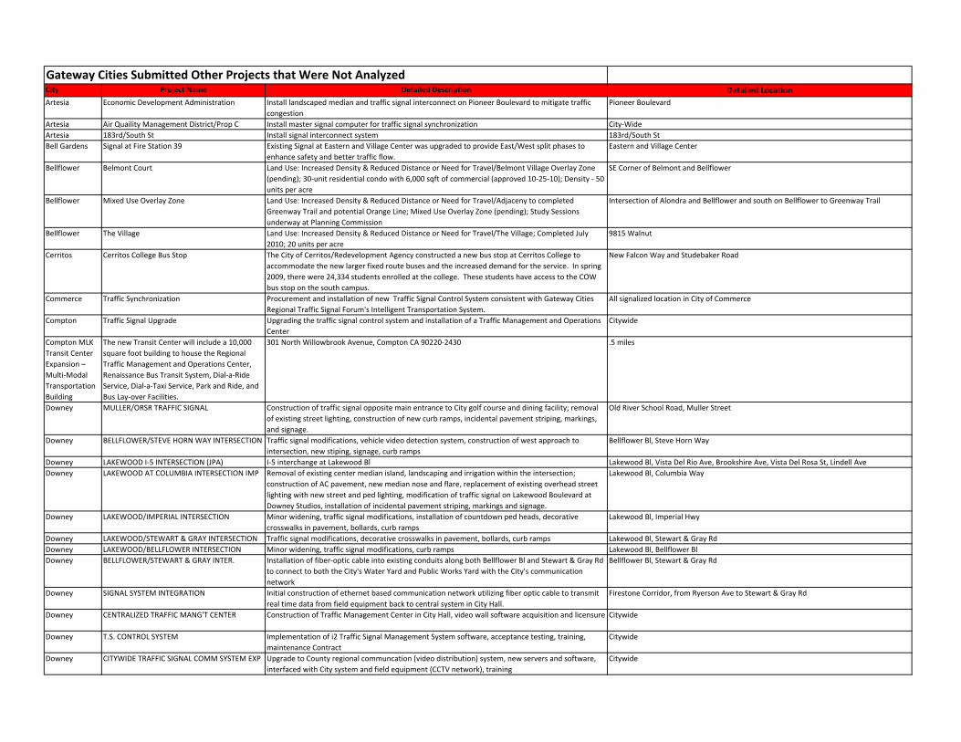
Gateway Cities Submitted Other Projects that Were Not AnalyzedCity Project Name Detailed Description Detailed Location
Artesia Economic Development Administration Install landscaped median and traffic signal interconnect on Pioneer Boulevard to mitigate traffic
congestion
Pioneer Boulevard
Artesia Air Quaility Management District/Prop C Install master signal computer for traffic signal synchronization City‐Wide
Artesia 183rd/South St Install signal interconnect system 183rd/South St
Bell Gardens Signal at Fire Station 39 Existing Signal at Eastern and Village Center was upgraded to provide East/West split phases to
enhance safety and better traffic flow.
Eastern and Village Center
Bellflower Belmont Court Land Use: Increased Density & Reduced Distance or Need for Travel/Belmont Village Overlay Zone
(pending); 30‐unit residential condo with 6,000 sqft of commercial (approved 10‐25‐10); Density ‐ 50
units per acre
SE Corner of Belmont and Bellflower
Bellflower Mixed Use Overlay Zone Land Use: Increased Density & Reduced Distance or Need for Travel/Adjaceny to completed
Greenway Trail and potential Orange Line; Mixed Use Overlay Zone (pending); Study Sessions
underway at Planning Commission
Intersection of Alondra and Bellflower and south on Bellflower to Greenway Trail
Bellflower The Village Land Use: Increased Density & Reduced Distance or Need for Travel/The Village; Completed July
2010; 20 units per acre
9815 Walnut
Cerritos Cerritos College Bus Stop The City of Cerritos/Redevelopment Agency constructed a new bus stop at Cerritos College to
accommodate the new larger fixed route buses and the increased demand for the service. In spring
2009, there were 24,334 students enrolled at the college. These students have access to the COW
bus stop on the south campus.
New Falcon Way and Studebaker Road
Commerce Traffic Synchronization Procurement and installation of new Traffic Signal Control System consistent with Gateway Cities
Regional Traffic Signal Forum's Intelligent Transportation System.
All signalized location in City of Commerce
Compton Traffic Signal Upgrade Upgrading the traffic signal control system and installation of a Traffic Management and Operations
Center
Citywide
Compton MLK
Transit Center
Expansion –
Multi‐Modal
Transportation
Building
The new Transit Center will include a 10,000
square foot building to house the Regional
Traffic Management and Operations Center,
Renaissance Bus Transit System, Dial‐a‐Ride
Service, Dial‐a‐Taxi Service, Park and Ride, and
Bus Lay‐over Facilities.
301 North Willowbrook Avenue, Compton CA 90220‐2430 .5 miles
Downey MULLER/ORSR TRAFFIC SIGNAL Construction of traffic signal opposite main entrance to City golf course and dining facility; removal
of existing street lighting, construction of new curb ramps, incidental pavement striping, markings,
and signage.
Old River School Road, Muller Street
Downey BELLFLOWER/STEVE HORN WAY INTERSECTION Traffic signal modifications, vehicle video detection system, construction of west approach to
intersection, new stiping, signage, curb ramps
Bellflower Bl, Steve Horn Way
Downey LAKEWOOD I‐5 INTERSECTION (JPA) I‐5 interchange at Lakewood Bl Lakewood Bl, Vista Del Rio Ave, Brookshire Ave, Vista Del Rosa St, Lindell Ave
Downey LAKEWOOD AT COLUMBIA INTERSECTION IMP Removal of existing center median island, landscaping and irrigation within the intersection;
construction of AC pavement, new median nose and flare, replacement of existing overhead street
lighting with new street and ped lighting, modification of traffic signal on Lakewood Boulevard at
Downey Studios, installation of incidental pavement striping, markings and signage.
Lakewood Bl, Columbia Way
Downey LAKEWOOD/IMPERIAL INTERSECTION Minor widening, traffic signal modifications, installation of countdown ped heads, decorative
crosswalks in pavement, bollards, curb ramps
Lakewood Bl, Imperial Hwy
Downey LAKEWOOD/STEWART & GRAY INTERSECTION Traffic signal modifications, decorative crosswalks in pavement, bollards, curb ramps Lakewood Bl, Stewart & Gray Rd
Downey LAKEWOOD/BELLFLOWER INTERSECTION Minor widening, traffic signal modifications, curb ramps Lakewood Bl, Bellflower Bl
Downey BELLFLOWER/STEWART & GRAY INTER. Installation of fiber‐optic cable into existing conduits along both Bellflower Bl and Stewart & Gray Rd
to connect to both the City's Water Yard and Public Works Yard with the City's communication
network
Bellflower Bl, Stewart & Gray Rd
Downey SIGNAL SYSTEM INTEGRATION Initial construction of ethernet based communication network utilizing fiber optic cable to transmit
real time data from field equipment back to central system in City Hall.
Firestone Corridor, from Ryerson Ave to Stewart & Gray Rd
Downey CENTRALIZED TRAFFIC MANG'T CENTER Construction of Traffic Management Center in City Hall, video wall software acquisition and licensure Citywide
Downey T.S. CONTROL SYSTEM Implementation of i2 Traffic Signal Management System software, acceptance testing, training,
maintenance Contract
Citywide
Downey CITYWIDE TRAFFIC SIGNAL COMM SYSTEM EXP Upgrade to County regional communcation (video distribution) system, new servers and software,
interfaced with City system and field equipment (CCTV network), training
Citywide

Gateway Cities Submitted Other Projects that Were Not AnalyzedCity Project Name Detailed Description Detailed Location
Downey DOWNEY ADVANCED TRAFFIC CONTROL
SYSTEM
Upgrade to County regional Information Exchange Network (IEN), new server and software,
interfaced with City i2 software and traffic signal management system, interfacing with field
equipment (controllers, switches, video cameras), training
Citywide
La Mirada La Mirada Signal Sync Signal Syncronization Rosecrans Ave, La Mirada Blvd, Imperial highway, Telegraph rd
Lakewood Housing Element Increase maximum residential density from 27 du/acre to 30 du/acre Citywide (multi‐family zones)
Lakewood ATCS Adaptive Traffic Control System installed on Five (5) Corridors in Lakewood. LADOT is the system
installed.
Lakewood Bus PAX Shelters 18 Passenger Bus Shelters added with solar lighting, benches and litter receptacles at various transit
stops.
Various transit stops.
Long Beach I‐405 & Orange Avenue Reconfigure off‐ramp and signalize to improve safety and capacity I‐405 & Orange Avenue
Long Beach I‐405 & Cherry Avenue Reconfigure on‐ramp to improve safety and capacity I‐405 & Cherry Avenue
Long Beach Anaheim Street & Oregon Avenue Reconfigure southbound intersection approach to reduce conflicts and modernize traffic signal to
improve peak traffic flow.
Anahiem Street & Oregon Avenue
Long Beach Millikan High School Transporation
Improvement Project
Modernize a traffic signal to address ADA issues, traffic congestion, and an ackward intersection jog,
thereby improving traffic operations and safety for residents and students.
Spring Street & Snowden Avenue
Long Beach Pacific Avenue & Spring Street Intersection
Enhancement Project
Intersection provides primary access across Blue Line tracks, to an adjacent park, and nearby
hospital. Improvements include pedestrian countdown signals, lighting improvements, and adaptive
control elements to address varrying traffic and emergency vheicle demands while providing traffic
calming elements off peak.
Pacific Avenue & Spring Street
Long Beach Orange Avenue/Alamitos Avenue Traffic
Improvement Project
Reconfigured a schewed roadway alignment to eliminate conflicts, concentrate pedestrian
movements, and provide traffic signal control.
Alamitos Avenue between 17th Street & 15th Street
Long Beach Virgina Village Transportation Enhancement
Project
Construct median, install two new traffic signals, convert cross streets to one‐way to reduce
conflicting traffic movements, enhance capacity, and improve safety
Long Beach Boulevard between Del Amo Boulevard and 55th Street
Long Beach Wardlow Road Transportation Improvement
Project
Complete gaps in sidewalks and modernize traffic signals to facilitate peak period traffic flow and
safety
Wardlow Road between Cherry Avenue & Long Beach Boulevard
Long Beach Atherton Transportation Improvement Project Modernize one traffic signal to provide left‐turn phasing and adaptive control and install a new
traffic signal to improve access for vehciles and pedestrians to improve traffic opeations between
freeway connections and CSULB.
Atherton Street between Studebaker Road & Bellflower Boulevard
Long Beach Iron Triangle Transporation Improvement
Project
Project to provide grade separation of a number of traffic movements at the primary access point
between freeways and the southeast area of the City
7th Street, Bellflower, & PCH triangle of intersections.
Long Beach Shoreline Adpative Traffic Signal Project Implement an Adaptive Traffic Signal Control system, including CCTV, CMS, and other motorist
information systems in downtown Long Beach to address peak period congestion and special events.
Downtown Long Beach
Long Beach Long Beach Traffic Management Center Construciton of a new regional TMC to operate traffic signals and motorist information systems for
the Cities of Long Beach, Lakewood, Signal Hill, Bellflower, Hawaiian Gardens, and some State owned
traffic signals/faclities
Long Beach City Hall
Long Beach Douglas Park ATCS Expansion Project Expansion of the recently completed 160 traffic signal Long Beach TLSP project to include
approximately 120 additonal traffic signals into the new system
8 Square Mile area comprising multiple jursdictions in the area bounded by I‐405, I‐605,
CA‐91, I‐710
Long Beach Orange Avenue Transportation Improvement
Project
A project to reduce conflicts and traffic operations adjacent to a new grocery market and fire station
underconstruction. Project involves a number of improvements to an existing traffic signal and the
installation of a new traffic signal.
Orange Avenue between CA‐91 and Artesia Boulevard
Lynwood Imperial Hwy and Martin Luther King Blvd.
Intersection Improvement Project
Truck impacted instersection. County project to widen curb returns, PCC intersection, traffic signal
improvements and sidewalk improvements.
Imperial Hwy and Martin Luther King Jr, Blvd.
Lynwood Long Beach Blvd Improvement Project Street improvement project including realignment and improve intersection geometry of Long Beach
Blvd., State Street and Tenaya Avenue.
Long Beach Blvd., State Street and Tenaya Avenue.
maywood Slauson @ Atlantic Intersection widening and concrete lanes Slauson @ Atlantic
Multiple install wireless communications for traffic signal system City of South Gate, Lynwood, Huntington Park, La Mirada, Commerce,
Multiple install wireless communications for traffic signal system City of Bell, Bell Gardens, Santa Fe Springs, Cudahy, Maywood, Pico Rivera, Paramount
Norwalk Project 7212 Replaced signal cabinet and upgraded traffic signal controller assembly, conduits, cables, and
electrical service
Pioneer Boulevard/Lakeland Road
Norwalk Firestone Boulevard Rehabilitation Extend 3rd WB lane. WB Firestone Boulevard at Target Driveway (west of I‐605 Freeway)
Norwalk Traffic Control System Installation of a traffic control system Citywide
Norwalk Traffic Control System Upgrade and expand traffic control system Citywide

Gateway Cities Submitted Other Projects that Were Not AnalyzedCity Project Name Detailed Description Detailed Location
Parmount Rosecrans and Anderson Vehicle video detection
Parmount Rosecrans and Bianchi Way Vehicle video detection
Parmount Somerset and Texaco Vehicle video detection
Parmount Somerset and Garfield Vehicle video detection
Parmount Somerset and Paramount Vehicle video detection
Parmount Somerset and Orizaba Vehicle video detection
Parmount Somerset and Downey Vehicle video detection
Parmount Downey and Gardendale Vehicle video detection
Parmount Rosecrans and Downey Vehicle video detection
Regionwide Charging Stations at Key Test Stations (Norwalk,
Long Beach)
VMT Reduction from Mode Shift at Stations that have EV Station Cars or Charging Stations. Research
to estimate mode shift for drivers of EV vehicles?
Region‐wide
Santa Fe
Springs
RTO for EB Telegraph at Bloomfield Ave. Installation of right turn only pocket for EB traffic at the intersection of Telegraph at Bloomfield Telegraph Rd. & Bloomfield Ave.
Santa Fe
Springs
Traffic Control System Installation of a traffic control system Citywide
Signal Hill Orange & Hill Street Bridge Overpass Removal Demo the bridge overpass at Hill & Orange intersection and remove existing grade separation Orange Ave & Hill Street
Signal Hill Cherry Ave and I‐405 Ramp Interchange Ramp Interchange improvement Cherry Ave & I‐405 interchange
Signal Hill 800 Crescent Heights Street Improvement Reconstruction of Gardena St Burnett to Crescent Heights Streets
Signal Hill 613 Nevada Street Reconstruct Orange to Cerritos
Signal Hill Patterson Street New Street segment California to Olive
Signal Hill Olive Street New Street segment Patterson to 27th
Signal Hill 28th Street New Street segment California to Olive
Signal Hill Olive Street New Street segment 28th to Patterson
Signal Hill 673 Orange Ave Signal Upgrades Replace traffic signals 32nd and 33rd Streets @ Orange Ave
Signal Hill Citywide bus stop improvements Install newly designed bus stops Citywide
South Gate 329‐ST Truck impacted intersection Phase II
Imperial Highway and Garfield Ave
This project will benift the city by improving the traffic flow conditions on Imperial Highway and
Garfield Avenue. The construction consists of widening the intersection that includes new curbs,
gutters, sidewalk and drainage system as well as upgrades of traffic signals.
Imperial Hwy, Garfield Ave
South Gate 365‐ST Atlantic Ave & Firestone Blvd
Intersection Improvements
Three thru lanes in each direction and a left turn lane is designated for arterial roadways. The
proposed improvements will be consistent with the General Plan. Provide a wider typical section in
order to realign the intersection.
Firestone Blvd, Atlantic Ave
South Gate 358‐ST Atlantic Ave Improvement Project Roadway pavement rehabilitation with asphalt rubber hot mix, construction landscaped median
island , sidewalk, curb, and gutter repairs, reconstruction of curb ramps to meet Americans with
Disabilities Act standards, signal interconnect between Tweedy Boulevard and Michigan Avenue and
traffic signal upgrades, and peripheral improvements.
Atlantic Ave and Tweedy Blvd, Atlantic and Michigan Ave.
South Gate 448‐TRF Traffic Signal Left Turn Phasing on
Firestone Blvd at Santa Fe, Long Beach,
California, Otis
design protected left turns for the 4 intersections, provide compliance with ADA as it relates to
access ramps at the 4 intersections, and synchronize the modified signals with the Firestone corridor
Firestone Blvd at Santa Fe Ave, Long Beach Blvd, California Ave, Otis St
South Gate Traffic Management Center Remodeling and upgrade space at the City Yard with work stations, TCS software, computers, video
display. Upon completion the TMC will contribute traffic data to the Information Exchange Network,
integrate traffic signals into the Traffic Control System, and develop coordination plans from
information gathered.
TMC construction at the City Yard, upgrades to approx. 40 intersections throught the City
South Gate 358‐ST Atlantic Ave Improvement Project Roadway pavement rehabilitation with asphalt rubber hot mix, construction landscaped median
island , sidewalk, curb, and gutter repairs, reconstruction of curb ramps to meet Americans with
Disabilities Act standards, signal interconnect between Tweedy Boulevard and Michigan Avenue and
traffic signal upgrades, and peripheral improvements.
Atlantic Ave and Tweedy Blvd, Atlantic and Michigan Ave.
South Gate 448‐TRF Traffic Signal Left Turn Phasing on
Firestone Blvd at Santa Fe, Long Beach,
California, Otis
design protected left turns for the 4 intersections, provide compliance with ADA as it relates to
access ramps at the 4 intersections, and synchronize the modified signals with the Firestone corridor
Firestone Blvd at Santa Fe Ave, Long Beach Blvd, California Ave, Otis St
South Gate Traffic Control System Installation of a traffic control system and Traffic Management Center Citywide

Gateway Cities Submitted Other Projects that Were Not AnalyzedCity Project Name Detailed Description Detailed Location
Vernon 26th St Bridge and Street Improvement Street
Bridge
Extend 26th Street by constructing a bridge over Atlantic Blvd. and construct a new street
(Pennington Way) from the bridge to Bandini Blvd. Installation of a new traffic. New street and
bridge provides an alternative roadway route to commuters to and from the City, as well as easing
the traffic congestion throughout the City, especially at the adjacent intersection of Atlantic Blvd.
and Bandini Blvd.
Project is located at the east end of the Vernon. New traffic signal installed at the newly
constructed intersection of Pennington Way and Bandini Blvd.
Vernon Traffic Control System Project Installation of a Traffic Control System in the City of Vernon to facilitate the synchronization of traffic
signals, integrate ITS systems and exchange real‐time data among ITS systems located across
jurisdictional boundaries.
Signalized intersections citywide.
Vernon 37th/Bandini Blvd. Traffic Signal
Synchronization Project
Synchronization and upgrade of traffic signals along 37th/Bandini Blvd. corridor. 37th St./Bandini Blvd. from Alameda to Pennington Way
Whittier Painter Avenue at Whittier Greenway Trail Installation of new Pedestrian signal Painter Aveue at Whittier Greenway Trail
Whittier Hadley Street at Whittier Greenway Trail/City
Yard
Installation of new traffic signal Hadley Street at Whittier Greenway Trail/City Yard
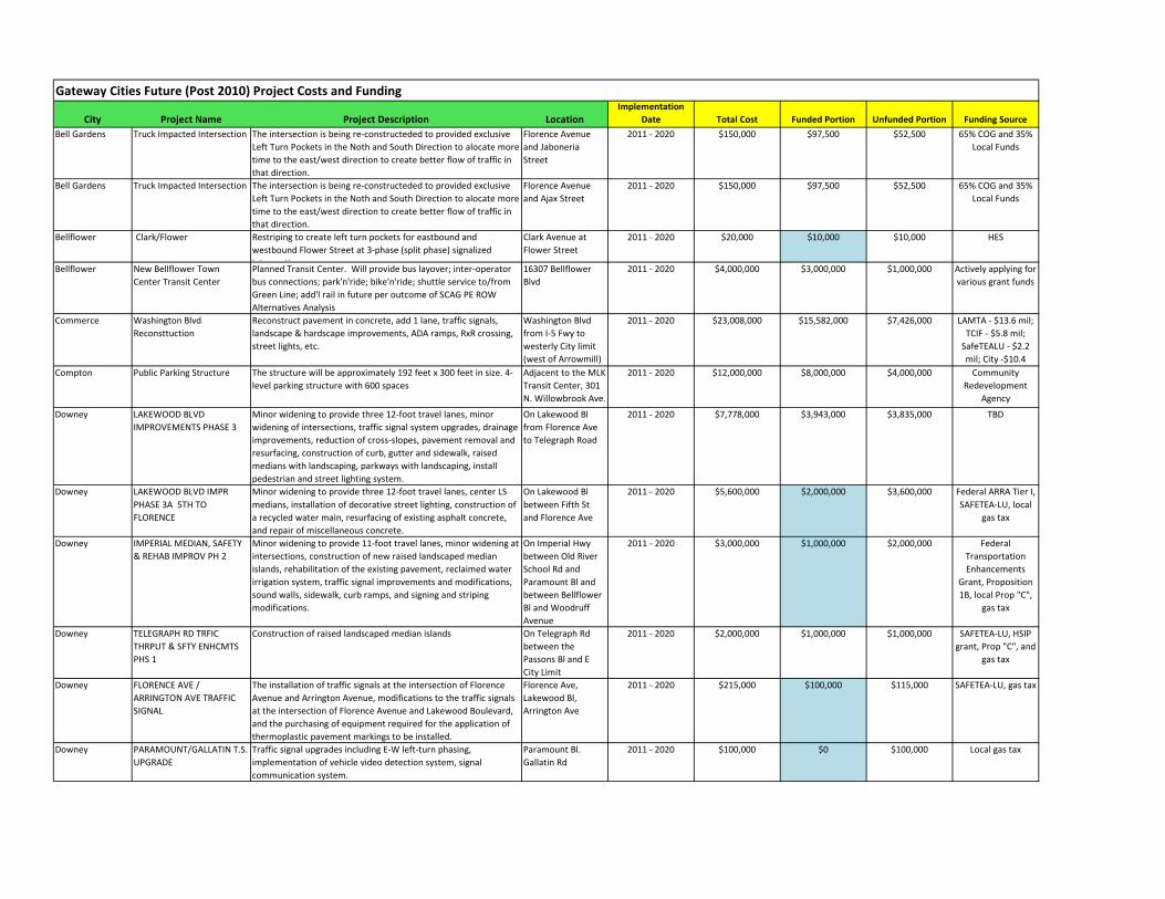
Gateway Cities Future (Post 2010) Project Costs and Funding
City Project Name Project Description LocationImplementation
Date Total Cost Funded Portion Unfunded Portion Funding Source
Bell Gardens Truck Impacted Intersection The intersection is being re‐constructeded to provided exclusive
Left Turn Pockets in the Noth and South Direction to alocate more
time to the east/west direction to create better flow of traffic in
that direction.
Florence Avenue
and Jaboneria
Street
2011 ‐ 2020 $150,000 $97,500 $52,500 65% COG and 35%
Local Funds
Bell Gardens Truck Impacted Intersection The intersection is being re‐constructeded to provided exclusive
Left Turn Pockets in the Noth and South Direction to alocate more
time to the east/west direction to create better flow of traffic in
that direction.
Florence Avenue
and Ajax Street
2011 ‐ 2020 $150,000 $97,500 $52,500 65% COG and 35%
Local Funds
Bellflower Clark/Flower Restriping to create left turn pockets for eastbound and
westbound Flower Street at 3‐phase (split phase) signalized
intersection
Clark Avenue at
Flower Street
2011 ‐ 2020 $20,000 $10,000 $10,000 HES
Bellflower New Bellflower Town
Center Transit Center
Planned Transit Center. Will provide bus layover; inter‐operator
bus connections; park'n'ride; bike'n'ride; shuttle service to/from
Green Line; add'l rail in future per outcome of SCAG PE ROW
Alternatives Analysis
16307 Bellflower
Blvd
2011 ‐ 2020 $4,000,000 $3,000,000 $1,000,000 Actively applying for
various grant funds
Commerce Washington Blvd
Reconsttuction
Reconstruct pavement in concrete, add 1 lane, traffic signals,
landscape & hardscape improvements, ADA ramps, RxR crossing,
street lights, etc.
Washington Blvd
from I‐5 Fwy to
westerly City limit
(west of Arrowmill)
2011 ‐ 2020 $23,008,000 $15,582,000 $7,426,000 LAMTA ‐ $13.6 mil;
TCIF ‐ $5.8 mil;
SafeTEALU ‐ $2.2
mil; City ‐$10.4
Compton Public Parking Structure The structure will be approximately 192 feet x 300 feet in size. 4‐
level parking structure with 600 spaces
Adjacent to the MLK
Transit Center, 301
N. Willowbrook Ave.
2011 ‐ 2020 $12,000,000 $8,000,000 $4,000,000 Community
Redevelopment
Agency
Downey LAKEWOOD BLVD
IMPROVEMENTS PHASE 3
Minor widening to provide three 12‐foot travel lanes, minor
widening of intersections, traffic signal system upgrades, drainage
improvements, reduction of cross‐slopes, pavement removal and
resurfacing, construction of curb, gutter and sidewalk, raised
medians with landscaping, parkways with landscaping, install
pedestrian and street lighting system.
On Lakewood Bl
from Florence Ave
to Telegraph Road
2011 ‐ 2020 $7,778,000 $3,943,000 $3,835,000 TBD
Downey LAKEWOOD BLVD IMPR Minor widening to provide three 12‐foot travel lanes, center LS On Lakewood Bl 2011 ‐ 2020 $5,600,000 $2,000,000 $3,600,000 Federal ARRA Tier I,
PHASE 3A 5TH TO
FLORENCE
medians, installation of decorative street lighting, construction of
a recycled water main, resurfacing of existing asphalt concrete,
and repair of miscellaneous concrete.
between Fifth St
and Florence Ave
SAFETEA‐LU, local
gas tax
Downey IMPERIAL MEDIAN, SAFETY
& REHAB IMPROV PH 2
Minor widening to provide 11‐foot travel lanes, minor widening at
intersections, construction of new raised landscaped median
islands, rehabilitation of the existing pavement, reclaimed water
irrigation system, traffic signal improvements and modifications,
sound walls, sidewalk, curb ramps, and signing and striping
modifications.
On Imperial Hwy
between Old River
School Rd and
Paramount Bl and
between Bellflower
Bl and Woodruff
Avenue
2011 ‐ 2020 $3,000,000 $1,000,000 $2,000,000 Federal
Transportation
Enhancements
Grant, Proposition
1B, local Prop "C",
gas tax
Downey TELEGRAPH RD TRFIC
THRPUT & SFTY ENHCMTS
PHS 1
Construction of raised landscaped median islands On Telegraph Rd
between the
Passons Bl and E
City Limit
2011 ‐ 2020 $2,000,000 $1,000,000 $1,000,000 SAFETEA‐LU, HSIP
grant, Prop "C", and
gas tax
Downey FLORENCE AVE /
ARRINGTON AVE TRAFFIC
SIGNAL
The installation of traffic signals at the intersection of Florence
Avenue and Arrington Avenue, modifications to the traffic signals
at the intersection of Florence Avenue and Lakewood Boulevard,
and the purchasing of equipment required for the application of
thermoplastic pavement markings to be installed.
Florence Ave,
Lakewood Bl,
Arrington Ave
2011 ‐ 2020 $215,000 $100,000 $115,000 SAFETEA‐LU, gas tax
Downey PARAMOUNT/GALLATIN T.S.
UPGRADE
Traffic signal upgrades including E‐W left‐turn phasing,
implementation of vehicle video detection system, signal
communication system.
Paramount Bl.
Gallatin Rd
2011 ‐ 2020 $100,000 $0 $100,000 Local gas tax
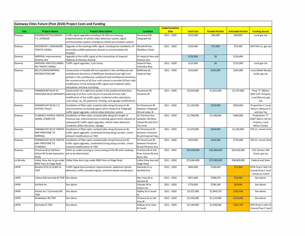
Gateway Cities Future (Post 2010) Project Costs and Funding
City Project Name Project Description LocationImplementation
Date Total Cost Funded Portion Unfunded Portion Funding Source
Downey PARAMOUNT/TELEGRAPH
T.S. UPGRADE
Traffic signal upgrades including E‐W left‐turn phasing,
implementation of vehicle video detection system, signal
communication system, emergency vehicle pre‐emption system.
Paramount Bl,
Telegraph Rd
2011 ‐ 2020 $120,000 $60,000 $60,000 Local gas tax
Downey WOODRUFF / WASHBURN
TRAFFIC SIGNAL
Upgrade of the existing traffic signal, including the installation of
accessible audible pedestrian devices to accommodate the
disabled
Woodruff Ave,
Washburn Road
2011 ‐ 2020 $150,000 $75,000 $75,000 SAFETEA‐LU, gas tax
Downey IMPERIAL Improvements,
Downey Ave
upgrade to the traffic signal at the intersection of Imperial
Highway at Downey Avenue.
At Imperial Hwy and
Downey Ave
$150,000 $0 $150,000
Downey IMPERIAL HWY/COLUMBIA
WY TRAFFIC SIGNAL
Traffic signal upgrades, curb ramps. Imperial Hwy,
Columbia Way
2011 ‐ 2020 $125,000 $0 $125,000 Local gas tax
Downey BELLFLOWER/IMPERIAL
INTERSECTION IMP
Construction of double left‐turn pockets in the northbound and
southbound directions on Bellflower Boulevard and right‐turn
pockets in the southbound, eastbound and northbound directions,
the reconstruction of all four curb returns to provide 50‐foot radii,
modification of the existing traffic signal and incidental utility
relocations and lane restriping
Bellflower Bl,
Imperial Hwy
2011 ‐ 2020 $210,000 $105,000 $105,000 Local (NASA Develp
fund), gas tax
Downey PARAMOUNT BLVD AT
FIRESTONE BLVD IMPRVMTS
Construction of a right‐turn pocket in the eastbound direction,
widening of all four curb returns to provide 50‐foot radii,
modification of the traffic signal, incidental utility relocations,
curb ramps, sw, AC pavement, striping, and signage modifications
Paramount Bl,
Firestone Bl
2011 ‐ 2020 $3,019,000 $1,822,000 $1,197,000 Prop "C" (Metro
2007 Call f Projects,
Local Return), gas
tax
Downey PARAMOUNT BLVD F.O.
SYSTEM, Phase I
Installation of fiber‐optic conduit/cable along Paramount Bl,
interconnection to existing signal comm network at Telegraph,
traffic signal upgrades, vehicle video detection system
On Paramount Bl
between Telegraph
Rd and Lubec St
2011 ‐ 2020 $1,150,000 $230,000 $920,000 Proposition C Local
Return, Measure R
and Gas Tax
Downey FLORENCE AVENUE TRAFFIC
SIGNAL COMM SYS
Installation of fiber‐optic conduit/cable along the length of
Florence Ave, interconnection to existing signal comm network at
Lakewood Bl, traffic signal upgrades, vehicle video detection,
incidental utility relocation, signage.
On Florence Ave
between Old River
School Rd and the E
City Limit
2011 ‐ 2020 $1,798,000 $1,438,000 $360,000 Proposition "C"
(2007 Metro Call for
Projects, Local
Return funds)
Downey PARAMOUNT BLVD TRAFFIC Installation of fiber‐optic conduit/cable along Paramount Bl, On Paramount Bl 2011 ‐ 2020 $1,670,000 $334,000 $1,336,000 TEA 21, transit fund
IMP‐FIRESTONE TO
IMPERIAL
traffic signal upgrades, coodinated timing along corridor, comm
network modifications at TMC
between Firestone
Bl and Imperial Hwy
Downey PARAMOUNT BLVD TRAFFIC
IMP‐FIRESTONE TO
FLORENCE
Installation of fiber‐optic conduit/cable along Paramount Bl,
traffic signal upgrades, coodinated timing along corridor, comm
network modifications at TMC
On Paramount Bl
between Firestone
Bl and Florence Ave
2011 ‐ 2020 $970,000 $194,000 $776,000 TEA 21, transit fund
Downey Firestone Bl at Old River
School Rd Grade Separation
Study
Either an undercrossing or overcrossing of the RR with roadway;
yet to be determined.
Firestone Bl at Old
River School Rd and
Burns Ave
2021 ‐ 2035 $59,500,000 $30,000,000 $29,500,000 PUC Section 190
Grant, gas tax
La Mirada Valley View Ave to go under
BNSF lines at Stage Road
Valley View Ave to go under BNSF lines at Stage Road Valley View Ave and
Stage Road
2011 ‐ 2020 $75,000,000 $37,000,000 $38,000,000 Federal and State
LAPW Bandini/37th St St/8th St
TSSP
Traffic Signal Syncronization improvements, additional vehicle
detection, traffic actuated signals, and time‐based coordination.
Alameda St to
Garfield Ave
2011 ‐ 2020 $844,000 $768,040 $75,960 MTA Prop C with LA
County Prop C local
money as match
LAPW Colima Rd/Lamirada Bl TSSP See above. Mar Vista Bl to
Alondra Bl
2011 ‐ 2020 $877,000 $798,070 $78,930 See above.
LAPW Garfield Av See above. Olympic Bl to
Eastern Av
2011 ‐ 2020 $776,000 $706,160 $69,840 See above.
LAPW Painter Av / Carmenita Rd
TSSP
See above. Hadley St to South
St
2011 ‐ 2020 $2,027,000 $1,844,570 $182,430 See above.
LAPW Studebaker Rd TSSP See above. Florence Av to Del
Amo Bl
2011 ‐ 2020 $1,226,000 $1,115,660 $110,340 See above.
LAPW Alameda St TSSP See above. Nadeau St to Auto
Dr South
2011 ‐ 2020 $2,130,000 $1,938,300 $191,700 MTA Prop C with LA
County Prop C local
t h

Gateway Cities Future (Post 2010) Project Costs and Funding
City Project Name Project Description LocationImplementation
Date Total Cost Funded Portion Unfunded Portion Funding Source
LAPW Woodruff Av TSSP See above. Firestone Av to
Willow St
2011 ‐ 2020 $2,491,350 $2,267,129 $224,222 See above.
LAPW Leffingwell Rd TSSP See above. Imperial Hwy to
Valley Home Av
2011 ‐ 2020 $929,000 $845,390 $83,610 See above.
LAPW Beverly Bl TSSP See above. Pomona Bl to
Pickering Av
2011 ‐ 2020 $2,393,000 $2,177,630 $215,370 See above.
LAPW South St TSSP See above. Atlantic Bl to
Studebaker Rd
2011 ‐ 2020 $1,485,000 $1,351,350 $133,650 See above.
LAPW Washington Bl TSSP See above. Atlantic Av to
Whittier Bl
2011 ‐ 2020 $2,341,000 $2,130,310 $210,690 See above.
LAPW Lambert Rd TSSP See above. Washington Bl to
Grayling Av
2011 ‐ 2020 $2,626,000 $2,389,660 $236,340 See above.
LAPW I‐710/Atlantic Corridor ITS
Project
See above. Alameda St from
Randolph Ave to
Industry Wy
2011 ‐ 2020 $3,226,000 $2,935,660 $290,340 See above.
LAPW I‐5 ATMS Integration Project See above. Imperial Hwy from
Carmenita Rd to
Valley View Ave;
Valley View Ave
from Imperial Hwy
to Rosecrans Ave
2011 ‐ 2020 $1,301,000 $1,183,910 $117,090 ISTEA DEMO and
Prop C local money
as match
Long Beach PCH & Cherry Cities of Long Beach & Signal Hill are working collectively to
acquire property to widen Cherry Avenue to add a second travel
lane in Long Beach from the Signal Hill boarder to south of PCH.
Cherry Avenue
between 19th
Street and 15th
2011 ‐ 2020 $6,721,000 $5,921,000 $800,000
Long Beach Walnut Avenue
Transportation
Enhancement Project
Reconfigure two separate intersections into a single intersection
and provide new signalized pedestrian crossings at a location that
serves four grade schools and adults accessing LBCC.
Walnut Avenue &
Alamitos/20th
Street
2011 ‐ 2020
$1,200,000 $800,000 $400,000 TMP/ SC25
Long Beach LCD Traffic Enhancement
Project
Reconfigure the LCD (LOS COYOTES DIAGONAL) & Studebaker
Road/Parkcrest intersection into two separate intersections to
LCD (LOS COYOTES
DIAGONAL)
2011 ‐ 2020 $2,500,000 $1,600,000 $900,000 TMP
improve traffic opeations and capacity while improving access to
a new high school currently underconstruction. Project also
includes reconfigeration of the lanes and traffic signal operations
at LCD & Carson Street to address peak period congestion issues.
between
Studebaker &
Carson Street
Long BeachDel Amo & Locust Intersectio
Signalize intersection to provide improved neighborhood
connectivity and access to tranist and park facilities
Del Amo Boulevard
& Locust Avenue
2011 ‐ 2020 $200,000 $0 $200,000 Gas tax
Long Beach
2nd Street & Pomona Avenue
Construction of a new traffic signal to facilitate traffic flow during
the peak period while also providing a new signalized pedestrian
crossing in a dense retail shopping center.
2nd Street &
Pomona Avenue
2011 ‐ 2020 $50,000 $0 $50,000 Parking meter
revenue
Long Beach Carson Street & Woodruff
Avenue Intersection
Improvement Project
Modernize traffic signal control and provide improved left‐turn
phasing to improve safety and operations
Carson Street &
Woodruff Avenue
2011 ‐ 2020 $35,000 $0 $35,000 TMP
Long Beach Spring Street & Woodruff
Avenue Intersection
Improvement Project
Modernize traffic signal to provide left‐turn phasing in two
directions and improved pedestrian crossings to address safety
and congestion issues.
Spring Street &
Woodruff Avenue
2011 ‐ 2020 $175,000 $0 $175,000 Gas tax
Long Beach PCH & Cherry Caltrans modernized the traffic signal to provide adaptive control
and left‐turn phasing to address congestion issues.
PCH & Cherry
Avenue
2011 ‐ 2020 $5,000,000 $3,000,000 $2,000,000 RDA / grant (sh)
Long Beach Redondo & Anahiem
Intersection Improvement
Widen Southbound Redondo Avenue to provide for right‐turn lane Redondo &
Anaheim
2011 ‐ 2020 $40,000 $26,000 $14,000 TMP
Long Beach PCH & 2nd Street
Improvement Project
Widen Southbound PCH to provide for 2nd left‐turn lane and right‐
turn lane
PCH & 2nd Street 2011 ‐ 2020 $3,000,000 $2,000,000 $1,000,000 TMP
Long Beach Los Alamitos Traffic Circle
Improvement Project
Cooperative Project with Caltrans to implement changes to the
traffic characteristics of the facility to improve capacity and
reduce accidents
PCH, Lakewood
Boulevard, LCD
2011 ‐ 2020 $2,000,000 $1,300,000 $700,000 state funds

Gateway Cities Future (Post 2010) Project Costs and Funding
City Project Name Project Description LocationImplementation
Date Total Cost Funded Portion Unfunded Portion Funding Source
Long Beach 2nd Street & Studebaker
Intersection Improvement
Project
Reconfigure intersection geometrics through the removal of a
median to add a third westbound travel lane
2nd Street &
Studebaker Road
2011 ‐ 2020 $400,000 $260,000 $140,000 TMP
Long Beach Ocean Boulevard
Transportation
Enhancement Project
Interconnect and modernize traffic signals along Ocean Boulevard
Corridor and add two new traffic signals to improve safety and
traffic operations
Ocean Boulevard
between Alamitos &
Livingston/2nd 2011 ‐ 2020
$1,280,000 $256,000 $1,024,000
Long Beach Atlantic Avenue
Transportation
Enhancement Project
Interconnect and modernize traffic signals along Atlantic Avenue
to improve operations and traffic safety
Atlantic Avenue
between Ocean
Boulevard &
Wardlow Road
2011 ‐ 2020
$1,080,000 $216,000 $864,000
Long Beach Studebaker Road ATCS and
Communictions
Enhancement Project
Construction of an eastside communications backbone to support
trafic signal control and motorist information systems, conversion
of traffic signal control from fixed time to adaptive control.
Studebaker Road
between Spring
Street and 2nd 2011 ‐ 2020
$1,080,000 $216,000 $864,000
Long Beach Wardlow Road Traffic Signal
Syncronization Project
Operational and timing improvements to traffic signals along the
Wardlow Road corridor in the western part of the City.
Wardlow Road
between Santa Fe &
the western City
li it
2011 ‐ 2020
$159,000 $31,000 $128,000
Long Beach 9th Street Pedestrian
Enhancement Project
Signalize two intersections and provide an all‐way stop at a third
to provide improved connectivity for pedestrians and cyclists
traveling along 9th Street to access schools, medical faclities, park
facilities, and shopping.
9th Street between
Pacific Avenue and
Long Beach
Boulevard
2011 ‐ 2020
$500,000 $385,000 $115,000
Long Beach Orange Avenue
Transportation
Improvement Project
Traffic Calming project to narrow the roadway via striping to
reduce vehicle speeds along this residential collector street and to
add a traffic signal midway to improve neighborhood connectivity
and access to transit stops.
Orange Avenue
between Wardlow
Road & Bixby Road2011 ‐ 2020
$350,000 $385,000 $115,000
Long Beach Walnut Avenue & 4th Street
Intersection Improvement
Modernize the traffic signal to provide enhanced pedestrian
access to bus stops and relocation of signal and electrical
equipment to improve pedestrian access to bus stops.
Walnut Avenue &
4th Street 2011 ‐ 2020
$150,000 $112,500 $27,500
Long Beach 3rd Street & Lime Avenue Construction of a new traffic signal in downtown to improve 3rd Street & Lime $175,000 $131,000 $44,000
Intersection Improvement pedestrain access to a nearby grocery market, schools, and transit
stops.
Avenue 2011 ‐ 2020
Long Beach Naples Road Diet Replaced one automobile lane with a Class II bicycle lane. Eastbound on 2nd
Street between
Bayshore Bridge and
Marina Drive
2011 ‐ 2020
$45,000 $34,000 $11,000
Long Beach Willow Street Pedestrian
Improvement
This project provides pedestrian‐oriented improvements to
Willow St including medians, pedestrian lighting, landscaping,
signage and crosswalk treatments.
Willow Street from
Los Angeles River to
Atlantic Avenue.
2011 ‐ 2020 $3,097,000 $2,180,000 $917,000 CMAQ
Local

Gateway Cities Future (Post 2010) Project Costs and Funding
City Project Name Project Description LocationImplementation
Date Total Cost Funded Portion Unfunded Portion Funding Source
Long Beach South Waterfront Bike Path
Connection
SWBPC project is the construction of a new Class I bike path
segment that closes an existing gap in the area. The project will
include a mid‐block crossing and wayfinding. This proposed path
closes a vital gap between the existing Class I path across
Queensway Bridge and the existing Class I bike and pedestrian
path along the south waterfront, connecting the Greater
Downtown with the hotels and commercial centers located across
the harbor.
The proposed South
Waterfront Bike
Path starts at the
north end of the
Queensway Bridge
at the existing
terminus of the
Class I path. The
proposed alignment
follows the north
side of Queensway
Drive within the City
right‐of‐way as a
Class I bike path to
the Special Events
Park existing Class I
2011 ‐ 2020 $1,500,000 $1,313,000 $187,000 CMAQ
Local
Long Beach 3rd Separated Bikeway Dedicated bike lanes on Broadway and 3rd will include a painted
island to separate the bike lane. One traffic lane will be lost to
preserve parking on both sides of the street.
3rd from Alamitos
and Golden Avenue
$940,000 $705,000 $195,000
Long Beach Broadway Separated
Bikeway
See above Broadway from
Alamitos and
Golden Avenue
$940,000 $705,000 $195,000
Long Beach Third Street Street Bike
Lanes
Bike lanes (Class II) along Third Street between Alamitos/Junipero
and Bike lane on Third Street b/w Alamitos/Junipero
Third Street
between
2011 ‐ 2020 $50,000 $37,500 $12,500
Long Beach Daisy Street ‐ Bike
Boulevard
Bike boulevard will provide North‐South Class III bicycle facility
(running the length of the City‐ from downtown to 70th).
running the length
of the City‐ from
downtown to 70th
2011 ‐ 2020 $2,200,000 $1,980,000 $220,000 CMAQ
SRTS
Long Beach Sixth Street ‐ Bike Boulevard Bike boulevard will provide East‐West Class III bicycle facility
(running from Junipero to Park).
6th St from Junipero
to Park
2011 ‐ 2020 $630,000 $567,000 $63,000 CMAQ
SRTS(running from Junipero to Park). to Park SRTS
Long Beach Market Street
Transporation Enhancement
Project
Reconfigure the roadway to provide improved pedestrian facilities
(widen sidewalks, enhanced pedestrian crossings) and access to
key destinations (post office, transit stops, fire station, schools,
shopping) for pedestrians, cylists, and motorists.
Market Street
between Long
Beach Boulevard
and Atlantic Avenue
2011 ‐ 2020 $5,000,000 $4,500,000 $500,000
Long Beach Long Beach Blvd. Pedestrian
Improvement Project
Project provides pedestrian‐oriented improvements to Long
Beach Boulevard including pedestrian lighting, street trees, and
crosswalk treatments.
Long Beach Blvd b/t
Willow Ave & I‐405
2011 ‐ 2020 $2,521,000 $1,722,000 $799,000 CMAQ
Local
Long Beach Atherton Street
Enhancement Project
Rehabilitating the landscaped median to enhance the experience
of over 37,000 pedestrians, bicyclists, transit users and autos
d l
Bellflower & Los
Cerritos Channel
2011 ‐ 2020 $1,322,000 $1,322,000 $0 CMAQ
Prop C
Long Beach San Gabriel River Bike Path
Closure at Willow Street
Creation of off‐street bicycle path to achieve bicycle route gap
closure on Willow Street from the San Gabriel River Bike Path
west to Studebaker Road
Willow St, at San
Gabriel River &
Studebaker
2011 ‐ 2020 $200,000 $150,000 $50,000 CMAQ
Local
Long Beach Harding Street Traffic
Calming Project
Reconfigure roadway stripping to install bike lanes and new
pedestrian crossings
Harding Street
between Atlantic
Avenue and Cherry
Avenue
2011 ‐ 2020 $1,200,000 $900,000 $300,000
Long Beach I‐710 Improvements Funded by the SAFETEA‐LU Demo Project, the project improves
bicycle, pedestrian, and streetscape on major thoroughfares.
On Broadway, 3rd
Street, 6th Street,
and 7th Street from
Shoreline Drive to
Alamitos.
2011 ‐ 2020 $2,000,000 $1,500,000 $500,000
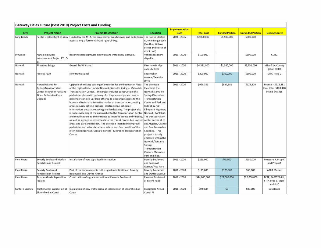
Gateway Cities Future (Post 2010) Project Costs and Funding
City Project Name Project Description LocationImplementation
Date Total Cost Funded Portion Unfunded Portion Funding Source
Long Beach Pacific Electric Right‐of‐Way Funded by the MTA, the project improves bikeway and pedestrian
access along a former railroad right‐of‐way.
The Pacific Electric
ROW in Long Beach
(South of Willow
Street and North of
4th Street)
2021 ‐ 2035 $2,000,000 $1,500,000 $500,000
Lynwood Annual Sidewalk
Improvement Project FY 10‐
11
Reconstructed damaged sidewalk and install new sidewalk. Various locations
citywide.
2011 ‐ 2020 $100,000 $100,000 CDBG
Norwalk Firestone Bridge Extend 3rd WB lane. Firestone Bridge
over SG River
2011 ‐ 2020 $4,331,000 $1,580,000 $2,751,000 MTA & LA County
grant, HBRR
PNorwalk Project 7219 New traffic signal Shoemaker
Avenue/Excelsior
Drive
2011 ‐ 2020 $200,000 $100,000 $100,000 MTA, Prop C
Norwalk Norwalk/Santa Fe
SpringsTransportation
Center‐Metrolink Park and
Ride ‐ Pedestrian Plaza
Upgrade
Upgrade of existing passenger amenities for the Pedestrian Plaza
at the regional inter‐modal Norwalk/Santa Fe Springs ‐ Metrolink
Transportation Center. The projec includes construction of a
pedestrian plaza with pathways for bicycles and pedestrians, a
passenger car pick‐up/drop‐off area to encourage access to the
buses and trains as alternative modes of transportation, seating
areas,security lighting, signage, electronic bus schedule
information, decorative paving and landscaping. The project also
includes widening of the approach into the Transportation Center
and modifications to the entrance to improve access and visibility,
as well as signage improvements to the transit center, bus layover
areas and park and ride lot. The project is intended to improve
pedestrian and vehicular access, safety, and functionality of the
inter‐modal Norwalk/SantaFe Springs ‐ Metrolink Transportation
Center.
The project is
located at the
Norwalk‐Santa Fe
SpringsIMetrolink
Transportation
Centerand Park and
Ride at 12700
E.lmperial Highway,
Norwalk, CA 90650.
The transportation
center serves all of
Los Angeles, Orange
and San Bernardino
Counties. This
project is totally
enclosed within the
2011 ‐ 2020 $966,351 $837,881 $128,470 Federal ‐ $612,881
local total $128,470
inkind $48,318
enclosed within the
Norwalk/Santa Fe
Springs
Transportation
Center ‐ Metrolink
Park and Ride.
Pico Rivera Beverly Boulevard Median
Rehabilitiaon Project
Installation of new signalized intersection Beverly Boulevard
and Sandoval
Avenue/Pico Park
2011 ‐ 2020 $225,000 $75,000 $150,000 Measure R, Prop C
and Prop 42
Pico Rivera Beverly Boulevard
Rehabilitaion Project
Part of the improvements Is the signal modification at Beverly
Boulevard and Durfee Avenue
Beverly Boulevard
and Durfee Avanue
2011 ‐ 2020 $175,000 $125,000 $50,000 ARRA Money
Pico Rivera Passons Grade Separation
Project
Construction of a grade separtion at Passons Boulevard Passons Boulevard
at Rivera Road
2011 ‐ 2020 $44,000,000 $22,000,000 $22,000,000 TCRP, SAFETEA‐LU,
STIP, Prop C, BNSF
and PUC
SantaFe Springs Traffic Signal Installation at
Bloomfield at Corral
Installation of new traffic signal at intersection of Bloomfield at
Corral
Bloomfield Ave. &
Corral Pl.
2011 ‐ 2020 $90,000 $0 $90,000 Developer

Gateway Cities Future (Post 2010) Project Costs and Funding
City Project Name Project Description LocationImplementation
Date Total Cost Funded Portion Unfunded Portion Funding Source
SantaFe Springs New Bike Lanes and Bike
Lockers
Bike lanes connecting Coyote Creek to Metrolink Transportation
Center and to San Gabriel River Path; and Bike lockers (total of 20
bike lockers) at Metrolink station
Foster Rd. to
Carmenita Rd. to
Orden Dr. west,
Leffingwell Rd.
north, to Adler Dr.
west, to Shoemaker
Av. north, to
Imperial Hwy. west,
to Transit Center,
then to Bloomfield
Ave. north, to Los
Nietos Rd. west, to
the San Gabriel
River bike path.
2011 ‐ 2020 $400,000 $320,000 $80,000 Federal Grant
Signal Hill 786 Cherry Ave Additional lanes 19th St to PCH 2011 ‐ 2020 $6,721,000 $5,921,000 $800,000 Traffic Impact Fees,
demo TE‐LU, MTA
Signal Hill California Avenue Reconstruction Patterson St to
Willow Avenue
2011 ‐ 2020 $508,000 $508,000
Signal Hill 746 Traffic Signal Cherry &
20th Street
New traffic signal (no signal or stop sign currently) Cherry Ave/ 20th St 2011 ‐ 2020 $750,000 $500,000 $250,000 Safe Routes to
School & Federal
Funds (HSIP)
Signal Hill Orizaba & PCH Traffic Signal New traffic signal Orizaba & PCH
intersection
2011 ‐ 2020 $250,000 $125,000 $125,000 Various Sources
Signal Hill Willow & Walnut Traffic
Signal
Left‐turn phasing traffic signal Willow & Walnut
intersection
2011 ‐ 2020 $120,000 $80,000 $40,000 Truck Impacted
Intersections South
Bay COG (MTA
Grants)
Signal Hill Willow & Orange Traffic Left‐turn phasing traffic signal Orange and Willow 2011 ‐ 2020 $370,000 $260,000 $110,000 Truck Impacted
Signal intersection Intersections South
Bay COG (MTA
Grants)
Signal Hill Orange Avenue Corridor
Traffic Signal
Synchronization
Synchronize traffic signals Spring Street to Hill
Street
$300,000 $60,000 $240,000 Gateway Cities
Traffic Forum
Signal Hill Citywide ADA Sidewalk
Improvements
Sidewalk improvements Citywide 2011 ‐ 2020 $100,000 $77,000 $23,000 CDBG
South Gate I‐710/Firestone Blvd
Interchange
This project involves widening south side of the Firestone
Boulevard Bridge over the Los Angles River to provide three
through lanes in each direction with a center raised median from
Rayo Ave to I‐710 freeway.
Firestone Boulevard
over LA River
2011 ‐ 2020 $14,721,000 $9,424,000 $5,297,000 Federal, Prop C

Gateway Cities Future (Post 2010) Project Costs and Funding
City Project Name Project Description LocationImplementation
Date Total Cost Funded Portion Unfunded Portion Funding Source
Vernon Atlantic Blvd. Bridge over
the LA River
The City of Vernon proposes to widen Atlantic Blvd. bridge over
the Los Angeles River. Project will enhance the safety and
operational use of Atlantic Blvd. bridge over the Los Angeles River
and improve the intersection performance at District Blvd. The
project involves widening Atlantic Blvd. for approximately 1,300
linear feet to provide traffic shoulders, standard sidewalks and
extending the right‐turn lane over to the Atlantic Blvd. Bridge. The
proposed roadway configuration includes six 11‐foot through
traffic lanes, one northbound 11‐foot right turn lane, 4‐foot
minimum shoulders, 5' sidewalks, and a center median. The
adjacent intersection of Atlantic Blvd. and District Blvd. will be
reconfigured and the traffic timing optimized.
Project limits are
from Atlantic Blvd.
north of the Los
Angeles River to 800
feet south of the
intersection with
District Blvd. The
proposed project is
located
approximately 0.25
miles (mi)
southwest of the
Long Beach Freeway
(1‐710) in the City of
Vernon
2011 ‐ 2020 $10,402,000 $3,602,000 $6,800,000 City Local and MTA
Funds
Vernon Atlantic Blvd. And District
Blvd Intersection
Improvement
The City of Vernon proposes to widen Atlantic Blvd. bridge over
the Los Angeles River. Project will enhance the safety and
operational use of Atlantic Blvd. bridge over the Los Angeles River
and improve the intersection performance at District Blvd. The
project involves widening Atlantic Blvd. for approximately 1,300
linear feet to provide traffic shoulders, standard sidewalks and
extending the right‐turn lane over to the Atlantic Blvd. Bridge. The
proposed roadway configuration includes six 11‐foot through
traffic lanes, one northbound 11‐foot right turn lane, 4‐foot
minimum shoulders, 5' sidewalks, and a center median. The
adjacent intersection of Atlantic Blvd. and District Blvd. will be
reconfigured and the traffic timing optimized.
Project limits are
from Atlantic Blvd.
north of the Los
Angeles River to 800
feet south of the
intersection with
District Blvd. The
proposed project is
located
approximately 0.25
miles (mi)
southwest of the
Long Beach Freeway
(1‐710) in the City of
V
2011 ‐ 2020 $6,800,000 $3,400,000 $3,400,000 City Local and MTA
Funds
VernonWhittier Hadley Street at Whittier
Avenue
Installation of new traffic signal Hadley Street at
Whittier Avenue
2011 ‐ 2020 $240,000 $120,000 $120,000 STPLG and Gas Tax
B
Whittier Lambert Road at Santa
Gertrudes Avenue
Traffic Signal Modification Lambert Road at
Santa Gertrudes
Avenue. Includes
installation of
median island to
separate traffic on
Santa Gertrudes
Avenue at adjacent
railroad grade
crossing.
2011 ‐ 2020 $535,000 $340,000 $195,000 HSIP Grant and
Proposition 1B
Whittier Lambert Road at Painter
Avenue
Traffic Signal Modification Lambert Road at
Painter Avenue
2011 ‐ 2020 $240,000 $120,000 $120,000 STPLG and Gas Tax
B
Whittier Lambert Road at Mills
Avenue
Traffic Signal Modification Lambert Road at
Mills Avenue. Joint
juridictional project
with Los Angeles
County. City 25%
share of project
cost.
2011 ‐ 2020 $131,500 $65,000 $66,500 STPLG

Gateway Cities Future (Post 2010) Project Costs and Funding
City Project Name Project Description LocationImplementation
Date Total Cost Funded Portion Unfunded Portion Funding Source
Whittier Pio Pico Bikeway
Connection
Bikeway connection from San Gabriel River Bike Path to the Pio
Pico State Histrocial Park
Adjacent to Whittier
Boulevard from San
Gabriel River Bike
Path to Pio Pico
State Historical Park
2011 ‐ 2020 $670,000 $536,000 $134,000 Rivers and
Mountains
Conservancy
Whittier Laurel Avenue Bike Lanes Installation of Class II Bike Lanes Laurel Avenue from
Whittier Blvd. to
Carnell Street
2006 ‐ 2010 $20,000 ARRA
Whittier Beverly Boulevard Class II
Bike Lanes
Installation of Class II Bike Lanes, Median Islands, Safety Lighting
and Bus Shelters
Beverly Blvd. from
605 Freeway to
Norwalk
Blvd/Workman Mill
Road.
2011 ‐ 2020 $1,242,500 $994,000 $248,500 HSIP and Propostion
1B
Whittier Mills Avenue Sidewalks Installation of Sidewalks and Wheelchair Access Ramps Mills Avenue from
Whittier Blvd. to
Lambert Road
2011 ‐ 2020 $425,000 $340,000 $85,000 SR2S and Gas Tax B
TOTAL $371,328,701 $215,296,720 $156,071,982
Note: Blue cells contain estimated costs. Orange cells contain per project cost averages devised from the FTIP in the case where multiple projects were funded as a single entity. Please see text for description of estimate methodology.
Appendix E. Analysis for Transportation Demand Management Strategies in the Gateway Cities
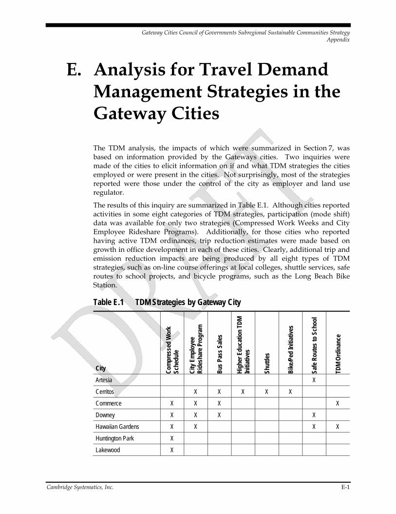
Gateway Cities Council of Governments Subregional Sustainable Communities Strategy Appendix
Cambridge Systematics, Inc. E-1
E. Analysis for Travel Demand Management Strategies in the Gateway Cities
The TDM analysis, the impacts of which were summarized in Section 7, was based on information provided by the Gateways cities. Two inquiries were made of the cities to elicit information on if and what TDM strategies the cities employed or were present in the cities. Not surprisingly, most of the strategies reported were those under the control of the city as employer and land use regulator.
The results of this inquiry are summarized in Table E.1. Although cities reported activities in some eight categories of TDM strategies, participation (mode shift) data was available for only two strategies (Compressed Work Weeks and City Employee Rideshare Programs). Additionally, for those cities who reported having active TDM ordinances, trip reduction estimates were made based on growth in office development in each of these cities. Clearly, additional trip and emission reduction impacts are being produced by all eight types of TDM strategies, such as on-line course offerings at local colleges, shuttle services, safe routes to school projects, and bicycle programs, such as the Long Beach Bike Station.
Table E.1 TDM Strategies by Gateway City
City Com
pres
sed
Wor
k Sc
hedu
le
City
Em
ploy
ee
Rid
esha
re P
rogr
am
Bus
Pas
s Sa
les
Hig
her E
duca
tion
TDM
In
itiat
ives
Shut
tles
Bik
e/Pe
d In
itiat
ives
Safe
Rou
tes
to S
choo
l
TDM
Ord
inan
ce
Artesia X
Cerritos X X X X X
Commerce X X X X
Downey X X X X
Hawaiian Gardens X X X X
Huntington Park X
Lakewood X

Gateway Cities Council of Governments Subregional Sustainable Communities Strategy Appendix
E-2 Cambridge Systematics, Inc.
City Com
pres
sed
Wor
k Sc
hedu
le
City
Em
ploy
ee
Rid
esha
re P
rogr
am
Bus
Pas
s Sa
les
Hig
her E
duca
tion
TDM
In
itiat
ives
Shut
tles
Bik
e/Pe
d In
itiat
ives
Safe
Rou
tes
to S
choo
l
TDM
Ord
inan
ce
La Mirada X X
Long Beach X X X X X X X
Lynwood X X
Pico Rivera X X X X X
Santa Fe Springs X X
Signal Hill X
Southgate X X X X X
Vernon X X X
Whittier X X X X X
The calculation of impacts for each of the three TDM strategies, for which mode shift or related data existed, is summarized below.
Compressed Work Weeks
Some 14 cities reported using compressed work week schedules for some or all of municipal employees. This is a very common strategy among South Coast Air Basin cities. While most cities used a 9/80 schedule, closing nonessential city office every other Friday, other cities employed 4/40 and 3/36 schedules.
In total, 3,309 employees are using a CWW schedule in the Gateway Cities. Most of these programs were implemented after 2005. The number of participants is not expected to grow in the planning years of 2020 and 2035. The calculation of GHG emission reduction impacts (in metric tons) is as follows:
Participating employees 3,309 (a)
Vehicle trip reduction (a x 80% prior SOV) 2,647 (b)
VMT reduction (b x 20 mile commute) 52,944 (c)
2020 GHG reduction (c x 327.36 g/mi) 17.3 tons per CWW day off (d)
2035 GHG reduction (c x 286.13 g/mi) 15.15 tons per CWW day off (e)

Gateway Cities Council of Governments Subregional Sustainable Communities Strategy Appendix
Cambridge Systematics, Inc. E-3
2020 GHG daily reduction (d x 14% of days are CWW days off) 2.43 tons per day (f)
2035 GHG daily reduction (e x 14%) 2.12 tons per day (g)
2020 GHG annual reduction (f x 250 commute days) 607.5 tons per year
2035 GHG annual reduction (g x 250 commute days) 530 tons per year
City Employee Ridesharing Program
Six cities reported having employee ridesharing programs for municipal workers. These cities reported that approximately 700 employees participated in the programs. Two of the cities reported an average vehicle ridership (AVR) of 1.29 and 1.31. Therefore, an AVR of 1.3 was applied to this employment and exemplary mode shares developed to equate to 1.3. This equated to a vehicle trip reduction of 418 trips. Assuming a 20-mile round trip commute, this equated to a VMT reduction of 8,360 miles. Applying the same emission factors cited above for CWW, this VMT reduction equates to a GHG emission reduction of 2.73 tons per day (2020) and 2.39 tons per day (2035). Annual reductions equate to 682.5 tons (2020) and 597.5 tons (2035). The diminishing reductions are due to lower emission factors in 2035 as California cars being cleaner and more efficient. City employee ridesharing participation was not expected to grow in future years.
TDM Ordinance
Eight cities reported having active TDM ordinances, seeking trip reduction mitigation at new commercial developments. While other cities presumably have TDM ordinances, they may not have reported due to inactivity of commercial development or with the ordinance application itself. The TDM ordinance analysis was different from that for Compressed Work Weeks and Employee Ridesharing, which had reported participation statistics. The known information related to this area was the existence of an ordinance and amount of estimated future office development in each city for 2020 and 2035 (from the SCAG Sustainability Tool).
First, trip reduction impacts were derived for new employment based on three scenarios: 1) a typical baseline mode split at office worksites, 2) an expected trip reduction of 8 percent due to the implementation of TDM strategies at new office developments (with the expected range of impacts from the most recent TDM literature – see Section 7), and 3) an expected trip reduction of 13 percent due to the interactive effects of TDM implemented at new developments, which are located in cities with aggressive smart growth and transit improvement policies and programs (see Section 10). These forecasted impacts were applied to a hypothetical group of 1,000 office workers and resulting mode splits were derived.
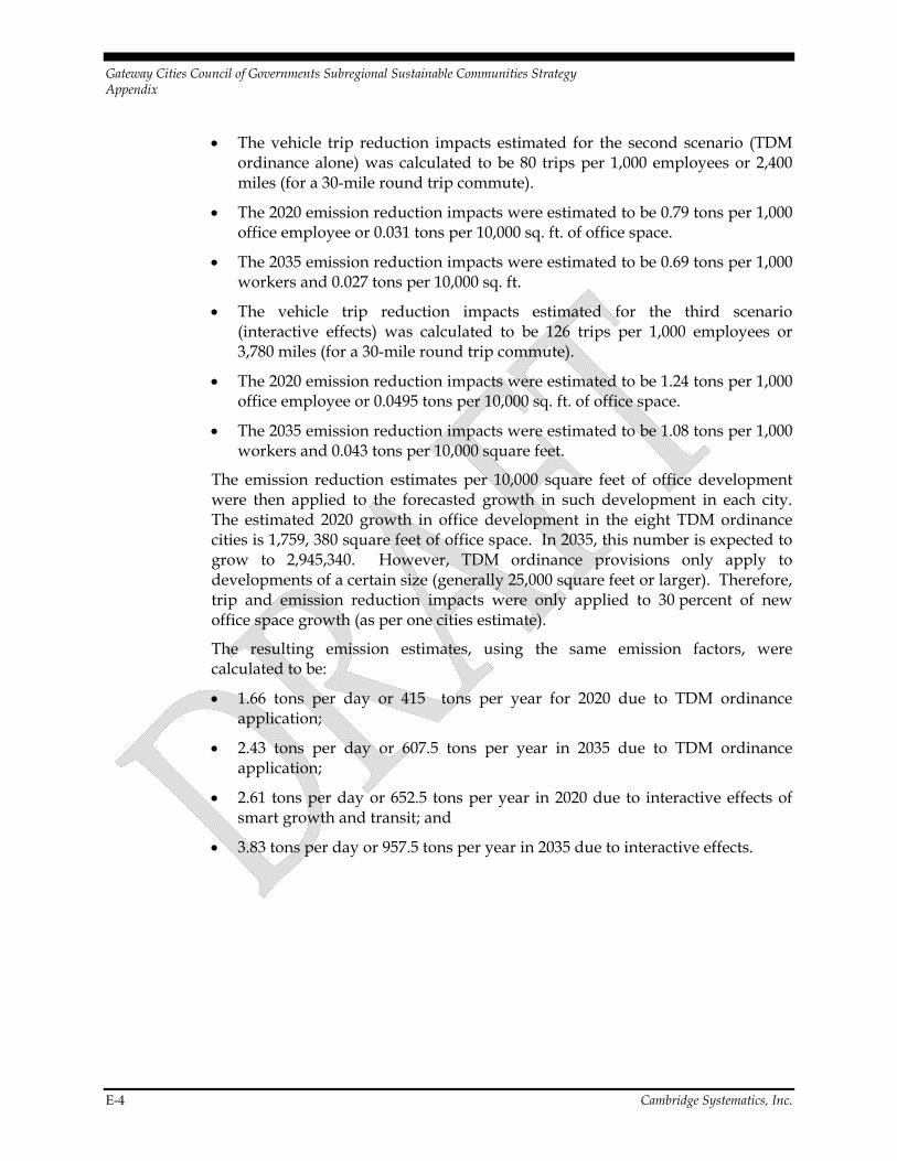
Gateway Cities Council of Governments Subregional Sustainable Communities Strategy Appendix
E-4 Cambridge Systematics, Inc.
The vehicle trip reduction impacts estimated for the second scenario (TDM ordinance alone) was calculated to be 80 trips per 1,000 employees or 2,400 miles (for a 30-mile round trip commute).
The 2020 emission reduction impacts were estimated to be 0.79 tons per 1,000 office employee or 0.031 tons per 10,000 sq. ft. of office space.
The 2035 emission reduction impacts were estimated to be 0.69 tons per 1,000 workers and 0.027 tons per 10,000 sq. ft.
The vehicle trip reduction impacts estimated for the third scenario (interactive effects) was calculated to be 126 trips per 1,000 employees or 3,780 miles (for a 30-mile round trip commute).
The 2020 emission reduction impacts were estimated to be 1.24 tons per 1,000 office employee or 0.0495 tons per 10,000 sq. ft. of office space.
The 2035 emission reduction impacts were estimated to be 1.08 tons per 1,000 workers and 0.043 tons per 10,000 square feet.
The emission reduction estimates per 10,000 square feet of office development were then applied to the forecasted growth in such development in each city. The estimated 2020 growth in office development in the eight TDM ordinance cities is 1,759, 380 square feet of office space. In 2035, this number is expected to grow to 2,945,340. However, TDM ordinance provisions only apply to developments of a certain size (generally 25,000 square feet or larger). Therefore, trip and emission reduction impacts were only applied to 30 percent of new office space growth (as per one cities estimate).
The resulting emission estimates, using the same emission factors, were calculated to be:
1.66 tons per day or 415 tons per year for 2020 due to TDM ordinance application;
2.43 tons per day or 607.5 tons per year in 2035 due to TDM ordinance application;
2.61 tons per day or 652.5 tons per year in 2020 due to interactive effects of smart growth and transit; and
3.83 tons per day or 957.5 tons per year in 2035 due to interactive effects.

Appendix F. Land Use Scenario Strategies from Sustainability Tool (2008, 2020, and 2035)

Acres
Rural Acres - 0% - 0% - 0% - 0% - 0%
Developed Acres 778 100% 778 100% 778 100% - 0% - 0%
Total 778 778 778 - -
ArtesiaScenario 5Scenario 1 Scenario 2 Scenario 3 Scenario 4
YR 2008 YR 2020 YR 2035
‐
500
1,000
Scenario 1 Scenario 2 Scenario 3 Scenario 4 Scenario 5
Acres Consumed
Developed Acres
Rural Acres
Housing Mix
Single Family 2,923 68% 2,979 67% 2,981 66% - 0% - 0%
Townhome - 0% - 0% - 0% - 0% - 0%
Multifamily 1,404 32% 1,440 33% 1,562 34% - 0% - 0%
Mobile Home - 0% - 0% - 0% - 0% - 0%
Total 4,327 4,419 4,543 - -
Employment Mix
‐
500
1,000
Scenario 1 Scenario 2 Scenario 3 Scenario 4 Scenario 5
Acres Consumed
Developed Acres
Rural Acres
‐
2,000
4,000
6,000
Scenario 1 Scenario 2 Scenario 3 Scenario 4 Scenario 5
Housing & Mix
Multifamily
Townhome
Single Family
Mobile Home
Jobs & MixEmployment Mix
Retail 1,877 32% 1,952 32% 2,016 31% - 0% - 0%
Office 3,497 59% 3,722 60% 3,926 61% - 0% - 0%
Industrial 517 9% 521 8% 518 8% - 0% - 0%
Total 5,891 6,195 6,460 - -
Density
Housing Unit 5.6 5.7 5.8 - -
‐
500
1,000
Scenario 1 Scenario 2 Scenario 3 Scenario 4 Scenario 5
Acres Consumed
Developed Acres
Rural Acres
‐
2,000
4,000
6,000
Scenario 1 Scenario 2 Scenario 3 Scenario 4 Scenario 5
Housing & Mix
Multifamily
Townhome
Single Family
Mobile Home
‐
5,000
10,000
Scenario 1 Scenario 2 Scenario 3 Scenario 4 Scenario 5
Jobs & Mix
Industrial
Office
Retail
60.0
VMT per Household
Employment 7.6 8.0 8.3 - -
Jobs/Housing Balance 1.4 1.4 1.4 - -
Vehicle Ownership per Household 2.2 2.2 2.2 - -
Vehicle Miles Traveled per Household 49.8 49.4 49.0 - -
Travel Mode Split
‐
500
1,000
Scenario 1 Scenario 2 Scenario 3 Scenario 4 Scenario 5
Acres Consumed
Developed Acres
Rural Acres
‐
2,000
4,000
6,000
Scenario 1 Scenario 2 Scenario 3 Scenario 4 Scenario 5
Housing & Mix
Multifamily
Townhome
Single Family
Mobile Home
‐
5,000
10,000
Scenario 1 Scenario 2 Scenario 3 Scenario 4 Scenario 5
Jobs & Mix
Industrial
Office
Retail
‐
20.0
40.0
60.0
Scenario 1 Scenario 2 Scenario 3 Scenario 4 Scenario 5
VMT per Household
100%
Travel Mode Split
Non Auto TripDrive Alone Trip 57.6% 57.7% 57.7% 0.0% 0.0%
Auto-Passenger Trip 29.0% 29.0% 28.9% 0.0% 0.0%
Transit Trip 4.1% 4.0% 4.0% 0.0% 0.0%
Non-Auto Trip 9.4% 9.4% 9.4% 0.0% 0.0%
Greenhouse Gas Emissions per Household
(Tons) 0.0222 0.0217 0.0218 - -
* GHG emissions per Household is calculated by dividing GHG emissions total (total VMT X Emission Factor) by the total number of households.
The below Emission Factors are for light‐ and medium‐duty vehicles only (excluding motorcycles) calculated with EMFACT model output based on 2008 RTP Amendment #3:
‐
500
1,000
Scenario 1 Scenario 2 Scenario 3 Scenario 4 Scenario 5
Acres Consumed
Developed Acres
Rural Acres
‐
2,000
4,000
6,000
Scenario 1 Scenario 2 Scenario 3 Scenario 4 Scenario 5
Housing & Mix
Multifamily
Townhome
Single Family
Mobile Home
‐
5,000
10,000
Scenario 1 Scenario 2 Scenario 3 Scenario 4 Scenario 5
Jobs & Mix
Industrial
Office
Retail
‐
20.0
40.0
60.0
Scenario 1 Scenario 2 Scenario 3 Scenario 4 Scenario 5
VMT per Household
0%
50%
100%
Scenario 1 Scenario 2 Scenario 3 Scenario 4 Scenario 5
Travel Mode Split
Non‐Auto Trip
Transit Trip
Auto‐Passenger Trip
Drive Alone Trip
The below Emission Factors are for light‐ and medium‐duty vehicles only (excluding motorcycles), calculated with EMFACT model output based on 2008 RTP Amendment #3:
Year 2008: 0.000446 tons per vmt
Year 2020: 0.000439 tons per vmt
Year 2035: 0.000445 tons per vmt
By default, emission factors for the years 2008, 2020, and 2035 are applied to calculate GHG emissions per Household values for Scenario 1~3 respectively (row 37 under columns B, D, F).

Acres
Vacant Acres 187 42% 726 70% 729 69% - 0% - 0%
Developed Acres 261 58% 305 30% 323 31% - 0% - 0%
Total 449 1,031 1,052 - -
AvalonScenario 5Scenario 1 Scenario 2 Scenario 3 Scenario 4
YR 2008 Existing YR 2035 Base YR2003 ALT1
‐
1,000
2,000
Scenario 1 Scenario 2 Scenario 3 Scenario 4 Scenario 5
Acres Consumed
Developed Acres
Vacant Acres
Housing Mix
Single Family 302 24% 349 24% 384 23% - 0% - 0%
Townhome - 0% - 0% - 0% - 0% - 0%
Multifamily 937 76% 1,095 76% 1,260 77% - 0% - 0%
Mobile Home - 0% - 0% - 0% - 0% - 0%
Total 1,239 1,444 1,644 - -
Employment Mix
‐
1,000
2,000
Scenario 1 Scenario 2 Scenario 3 Scenario 4 Scenario 5
Acres Consumed
Developed Acres
Vacant Acres
‐
1,000
2,000
Scenario 1 Scenario 2 Scenario 3 Scenario 4 Scenario 5
Housing & Mix
Multifamily
Townhome
Single Family
Mobile Home
Jobs & MixEmployment Mix
Retail 1,773 41% 1,842 39% 1,931 39% - 0% - 0%
Office 1,747 40% 1,997 43% 2,092 43% - 0% - 0%
Industrial 857 20% 857 18% 898 18% - 0% - 0%
Total 4,377 4,696 4,921 - -
Density
Housing Unit 2.8 1.4 1.6 - -
‐
1,000
2,000
Scenario 1 Scenario 2 Scenario 3 Scenario 4 Scenario 5
Acres Consumed
Developed Acres
Vacant Acres
‐
1,000
2,000
Scenario 1 Scenario 2 Scenario 3 Scenario 4 Scenario 5
Housing & Mix
Multifamily
Townhome
Single Family
Mobile Home
‐
2,000
4,000
6,000
Scenario 1 Scenario 2 Scenario 3 Scenario 4 Scenario 5
Jobs & Mix
Industrial
Office
Retail
50.0
VMT per Household
Employment 9.8 4.6 4.7 - -
Jobs/Housing Balance 3.5 3.3 3.0 - -
Vehicle Ownership per Household 1.6 1.6 1.6 - -
Vehicle Miles Traveled per Household 39.6 39.5 39.5 - -
Travel Mode Split
‐
1,000
2,000
Scenario 1 Scenario 2 Scenario 3 Scenario 4 Scenario 5
Acres Consumed
Developed Acres
Vacant Acres
‐
1,000
2,000
Scenario 1 Scenario 2 Scenario 3 Scenario 4 Scenario 5
Housing & Mix
Multifamily
Townhome
Single Family
Mobile Home
‐
2,000
4,000
6,000
Scenario 1 Scenario 2 Scenario 3 Scenario 4 Scenario 5
Jobs & Mix
Industrial
Office
Retail
‐
10.0
20.0
30.0
40.0
50.0
Scenario 1 Scenario 2 Scenario 3 Scenario 4 Scenario 5
VMT per Household
100%
Travel Mode Split
Non Auto TripDrive Alone Trip 54.5% 54.6% 54.3% 0.0% 0.0%
Auto-Passenger Trip 26.2% 26.2% 26.2% 0.0% 0.0%
Transit Trip 4.6% 4.6% 4.7% 0.0% 0.0%
Non-Auto Trip 14.6% 14.6% 14.9% 0.0% 0.0%
Greenhouse Gas Emissions per Household
(Tons) 0.0177 0.0176 0.0176 - -
‐
1,000
2,000
Scenario 1 Scenario 2 Scenario 3 Scenario 4 Scenario 5
Acres Consumed
Developed Acres
Vacant Acres
‐
1,000
2,000
Scenario 1 Scenario 2 Scenario 3 Scenario 4 Scenario 5
Housing & Mix
Multifamily
Townhome
Single Family
Mobile Home
‐
2,000
4,000
6,000
Scenario 1 Scenario 2 Scenario 3 Scenario 4 Scenario 5
Jobs & Mix
Industrial
Office
Retail
‐
10.0
20.0
30.0
40.0
50.0
Scenario 1 Scenario 2 Scenario 3 Scenario 4 Scenario 5
VMT per Household
0%
50%
100%
Scenario 1 Scenario 2 Scenario 3 Scenario 4 Scenario 5
Travel Mode Split
Non‐Auto Trip
Transit Trip
Auto‐Passenger Trip
Drive Alone Trip
* GHG emissions per Household is calculated by dividing GHG emissions total (total VMT X Emission Factor) by the total number of households.
The below Emission Factors are for light‐ and medium‐duty vehicles only (excluding motorcycles) calculated with EMFACT model output based on 2008 RTP Amendment #3: The below Emission Factors are for light‐ and medium‐duty vehicles only (excluding motorcycles), calculated with EMFACT model output based on 2008 RTP Amendment #3:
Year 2008: 0.000446 tons per vmt
Year 2020: 0.000439 tons per vmt
Year 2035: 0.000445 tons per vmt
By default, emission factors for the years 2008, 2020, and 2035 are applied to calculate GHG emissions per Household values for Scenario 1~3 respectively (row 37 under columns B, D, F).

Acres
Rural Acres 2 0% 3 0% 3 0% - 0% - 0%
Developed Acres 1,266 100% 1,283 100% 1,283 100% - 0% - 0%
Total 1,267 1,286 1,286 - -
BellScenario 5Scenario 1 Scenario 2 Scenario 3 Scenario 4
YR 2008 YR 2020 YR 2035
‐
1,000
2,000
Scenario 1 Scenario 2 Scenario 3 Scenario 4 Scenario 5
Acres Consumed
Developed Acres
Rural Acres
Housing Mix
Single Family 3,502 39% 3,502 39% 3,502 38% - 0% - 0%
Townhome - 0% - 0% - 0% - 0% - 0%
Multifamily 5,489 61% 5,540 61% 5,595 62% - 0% - 0%
Mobile Home - 0% - 0% - 0% - 0% - 0%
Total 8,991 9,042 9,097 - -
Employment Mix
‐
1,000
2,000
Scenario 1 Scenario 2 Scenario 3 Scenario 4 Scenario 5
Acres Consumed
Developed Acres
Rural Acres
‐
5,000
10,000
Scenario 1 Scenario 2 Scenario 3 Scenario 4 Scenario 5
Housing & Mix
Multifamily
Townhome
Single Family
Mobile Home
Jobs & MixEmployment Mix
Retail 3,010 34% 3,267 34% 3,475 35% - 0% - 0%
Office 3,103 35% 3,427 36% 3,716 37% - 0% - 0%
Industrial 2,856 32% 2,821 30% 2,773 28% - 0% - 0%
Total 8,969 9,515 9,964 - -
Density
Housing Unit 7.1 7.0 7.1 - -
‐
1,000
2,000
Scenario 1 Scenario 2 Scenario 3 Scenario 4 Scenario 5
Acres Consumed
Developed Acres
Rural Acres
‐
5,000
10,000
Scenario 1 Scenario 2 Scenario 3 Scenario 4 Scenario 5
Housing & Mix
Multifamily
Townhome
Single Family
Mobile Home
‐
5,000
10,000
15,000
Scenario 1 Scenario 2 Scenario 3 Scenario 4 Scenario 5
Jobs & Mix
Industrial
Office
Retail
50.0
VMT per Household
Employment 7.1 7.4 7.7 - -
Jobs/Housing Balance 1.0 1.1 1.1 - -
Vehicle Ownership per Household 1.9 1.9 1.9 - -
Vehicle Miles Traveled per Household 39.6 39.2 39.2 - -
Travel Mode Split
‐
1,000
2,000
Scenario 1 Scenario 2 Scenario 3 Scenario 4 Scenario 5
Acres Consumed
Developed Acres
Rural Acres
‐
5,000
10,000
Scenario 1 Scenario 2 Scenario 3 Scenario 4 Scenario 5
Housing & Mix
Multifamily
Townhome
Single Family
Mobile Home
‐
5,000
10,000
15,000
Scenario 1 Scenario 2 Scenario 3 Scenario 4 Scenario 5
Jobs & Mix
Industrial
Office
Retail
‐
10.0
20.0
30.0
40.0
50.0
Scenario 1 Scenario 2 Scenario 3 Scenario 4 Scenario 5
VMT per Household
100%
Travel Mode Split
Non Auto TripDrive Alone Trip 46.2% 46.2% 46.2% 0.0% 0.0%
Auto-Passenger Trip 32.0% 32.0% 32.0% 0.0% 0.0%
Transit Trip 6.1% 6.0% 6.0% 0.0% 0.0%
Non-Auto Trip 15.7% 15.7% 15.7% 0.0% 0.0%
Greenhouse Gas Emissions per Household
(Tons) 0.0177 0.0172 0.0174 - -
* GHG emissions per Household is calculated by dividing GHG emissions total (total VMT X Emission Factor) by the total number of households.
The below Emission Factors are for light‐ and medium‐duty vehicles only (excluding motorcycles) calculated with EMFACT model output based on 2008 RTP Amendment #3:
‐
1,000
2,000
Scenario 1 Scenario 2 Scenario 3 Scenario 4 Scenario 5
Acres Consumed
Developed Acres
Rural Acres
‐
5,000
10,000
Scenario 1 Scenario 2 Scenario 3 Scenario 4 Scenario 5
Housing & Mix
Multifamily
Townhome
Single Family
Mobile Home
‐
5,000
10,000
15,000
Scenario 1 Scenario 2 Scenario 3 Scenario 4 Scenario 5
Jobs & Mix
Industrial
Office
Retail
‐
10.0
20.0
30.0
40.0
50.0
Scenario 1 Scenario 2 Scenario 3 Scenario 4 Scenario 5
VMT per Household
0%
50%
100%
Scenario 1 Scenario 2 Scenario 3 Scenario 4 Scenario 5
Travel Mode Split
Non‐Auto Trip
Transit Trip
Auto‐Passenger Trip
Drive Alone Trip
The below Emission Factors are for light‐ and medium‐duty vehicles only (excluding motorcycles), calculated with EMFACT model output based on 2008 RTP Amendment #3:
Year 2008: 0.000446 tons per vmt
Year 2020: 0.000439 tons per vmt
Year 2035: 0.000445 tons per vmt
By default, emission factors for the years 2008, 2020, and 2035 are applied to calculate GHG emissions per Household values for Scenario 1~3 respectively (row 37 under columns B, D, F).

Acres
Rural Acres 29 1% 63 2% 63 2% - 0% - 0%
Developed Acres 3,511 99% 3,633 98% 3,633 98% - 0% - 0%
Total 3,541 3,696 3,696 - -
BellflowerScenario 5Scenario 1 Scenario 2 Scenario 3 Scenario 4
YR 2008 YR 2020 YR 2035
‐
2,000
4,000
Scenario 1 Scenario 2 Scenario 3 Scenario 4 Scenario 5
Acres Consumed
Developed Acres
Rural Acres
Housing Mix
Single Family 12,547 76% 13,220 75% 13,567 72% - 0% - 0%
Townhome - 0% - 0% - 0% - 0% - 0%
Multifamily 4,068 24% 4,460 25% 5,177 28% - 0% - 0%
Mobile Home - 0% - 0% - 0% - 0% - 0%
Total 16,615 17,680 18,744 - -
Employment Mix
‐
2,000
4,000
Scenario 1 Scenario 2 Scenario 3 Scenario 4 Scenario 5
Acres Consumed
Developed Acres
Rural Acres
‐
10,000
20,000
Scenario 1 Scenario 2 Scenario 3 Scenario 4 Scenario 5
Housing & Mix
Multifamily
Townhome
Single Family
Mobile Home
Jobs & MixEmployment Mix
Retail 8,245 51% 8,645 51% 8,936 51% - 0% - 0%
Office 4,965 31% 5,311 32% 5,689 33% - 0% - 0%
Industrial 2,922 18% 2,893 17% 2,875 16% - 0% - 0%
Total 16,132 16,849 17,500 - -
Density
Housing Unit 4.7 4.8 5.1 - -
‐
2,000
4,000
Scenario 1 Scenario 2 Scenario 3 Scenario 4 Scenario 5
Acres Consumed
Developed Acres
Rural Acres
‐
10,000
20,000
Scenario 1 Scenario 2 Scenario 3 Scenario 4 Scenario 5
Housing & Mix
Multifamily
Townhome
Single Family
Mobile Home
‐
10,000
20,000
Scenario 1 Scenario 2 Scenario 3 Scenario 4 Scenario 5
Jobs & Mix
Industrial
Office
Retail
60.0
VMT per Household
Employment 4.6 4.6 4.7 - -
Jobs/Housing Balance 1.0 1.0 0.9 - -
Vehicle Ownership per Household 2.2 2.2 2.2 - -
Vehicle Miles Traveled per Household 48.6 48.1 47.8 - -
Travel Mode Split
‐
2,000
4,000
Scenario 1 Scenario 2 Scenario 3 Scenario 4 Scenario 5
Acres Consumed
Developed Acres
Rural Acres
‐
10,000
20,000
Scenario 1 Scenario 2 Scenario 3 Scenario 4 Scenario 5
Housing & Mix
Multifamily
Townhome
Single Family
Mobile Home
‐
10,000
20,000
Scenario 1 Scenario 2 Scenario 3 Scenario 4 Scenario 5
Jobs & Mix
Industrial
Office
Retail
‐
20.0
40.0
60.0
Scenario 1 Scenario 2 Scenario 3 Scenario 4 Scenario 5
VMT per Household
100%
Travel Mode Split
Non Auto TripDrive Alone Trip 54.8% 54.8% 54.7% 0.0% 0.0%
Auto-Passenger Trip 30.4% 30.5% 30.5% 0.0% 0.0%
Transit Trip 4.2% 4.2% 4.2% 0.0% 0.0%
Non-Auto Trip 10.5% 10.5% 10.6% 0.0% 0.0%
Greenhouse Gas Emissions per Household
(Tons) 0.0217 0.0211 0.0213 - -
* GHG emissions per Household is calculated by dividing GHG emissions total (total VMT X Emission Factor) by the total number of households.
The below Emission Factors are for light‐ and medium‐duty vehicles only (excluding motorcycles) calculated with EMFACT model output based on 2008 RTP Amendment #3:
‐
2,000
4,000
Scenario 1 Scenario 2 Scenario 3 Scenario 4 Scenario 5
Acres Consumed
Developed Acres
Rural Acres
‐
10,000
20,000
Scenario 1 Scenario 2 Scenario 3 Scenario 4 Scenario 5
Housing & Mix
Multifamily
Townhome
Single Family
Mobile Home
‐
10,000
20,000
Scenario 1 Scenario 2 Scenario 3 Scenario 4 Scenario 5
Jobs & Mix
Industrial
Office
Retail
‐
20.0
40.0
60.0
Scenario 1 Scenario 2 Scenario 3 Scenario 4 Scenario 5
VMT per Household
0%
50%
100%
Scenario 1 Scenario 2 Scenario 3 Scenario 4 Scenario 5
Travel Mode Split
Non‐Auto Trip
Transit Trip
Auto‐Passenger Trip
Drive Alone Trip
The below Emission Factors are for light‐ and medium‐duty vehicles only (excluding motorcycles), calculated with EMFACT model output based on 2008 RTP Amendment #3:
Year 2008: 0.000446 tons per vmt
Year 2020: 0.000439 tons per vmt
Year 2035: 0.000445 tons per vmt
By default, emission factors for the years 2008, 2020, and 2035 are applied to calculate GHG emissions per Household values for Scenario 1~3 respectively (row 37 under columns B, D, F).

Acres
Rural Acres 25 2% 26 2% 26 2% - 0% - 0%
Developed Acres 1,057 98% 1,093 98% 1,093 98% - 0% - 0%
Total 1,081 1,119 1,119 - -
Bell GardensScenario 5Scenario 1 Scenario 2 Scenario 3 Scenario 4
YR 2008 YR 2020 YR 2035
‐
1,000
2,000
Scenario 1 Scenario 2 Scenario 3 Scenario 4 Scenario 5
Acres Consumed
Developed Acres
Rural Acres
Housing Mix
Single Family 4,488 47% 4,488 47% 4,488 46% - 0% - 0%
Townhome - 0% - 0% - 0% - 0% - 0%
Multifamily 5,110 53% 5,154 53% 5,201 54% - 0% - 0%
Mobile Home - 0% - 0% - 0% - 0% - 0%
Total 9,598 9,642 9,689 - -
Employment Mix
‐
1,000
2,000
Scenario 1 Scenario 2 Scenario 3 Scenario 4 Scenario 5
Acres Consumed
Developed Acres
Rural Acres
‐
5,000
10,000
15,000
Scenario 1 Scenario 2 Scenario 3 Scenario 4 Scenario 5
Housing & Mix
Multifamily
Townhome
Single Family
Mobile Home
Jobs & MixEmployment Mix
Retail 3,087 38% 3,297 38% 3,463 38% - 0% - 0%
Office 3,428 42% 3,786 44% 4,111 45% - 0% - 0%
Industrial 1,564 19% 1,566 18% 1,567 17% - 0% - 0%
Total 8,079 8,650 9,141 - -
Density
Housing Unit 8.9 8.6 8.7 - -
‐
1,000
2,000
Scenario 1 Scenario 2 Scenario 3 Scenario 4 Scenario 5
Acres Consumed
Developed Acres
Rural Acres
‐
5,000
10,000
15,000
Scenario 1 Scenario 2 Scenario 3 Scenario 4 Scenario 5
Housing & Mix
Multifamily
Townhome
Single Family
Mobile Home
‐
5,000
10,000
Scenario 1 Scenario 2 Scenario 3 Scenario 4 Scenario 5
Jobs & Mix
Industrial
Office
Retail
50.0
VMT per Household
Employment 7.5 7.7 8.2 - -
Jobs/Housing Balance 0.8 0.9 0.9 - -
Vehicle Ownership per Household 2.0 2.0 2.0 - -
Vehicle Miles Traveled per Household 43.0 41.3 41.2 - -
Travel Mode Split
‐
1,000
2,000
Scenario 1 Scenario 2 Scenario 3 Scenario 4 Scenario 5
Acres Consumed
Developed Acres
Rural Acres
‐
5,000
10,000
15,000
Scenario 1 Scenario 2 Scenario 3 Scenario 4 Scenario 5
Housing & Mix
Multifamily
Townhome
Single Family
Mobile Home
‐
5,000
10,000
Scenario 1 Scenario 2 Scenario 3 Scenario 4 Scenario 5
Jobs & Mix
Industrial
Office
Retail
‐
10.0
20.0
30.0
40.0
50.0
Scenario 1 Scenario 2 Scenario 3 Scenario 4 Scenario 5
VMT per Household
100%
Travel Mode Split
Non Auto TripDrive Alone Trip 44.6% 44.7% 44.7% 0.0% 0.0%
Auto-Passenger Trip 33.9% 34.0% 33.9% 0.0% 0.0%
Transit Trip 5.9% 5.7% 5.7% 0.0% 0.0%
Non-Auto Trip 15.7% 15.7% 15.7% 0.0% 0.0%
Greenhouse Gas Emissions per Household
(Tons) 0.0192 0.0181 0.0183 - -
* GHG emissions per Household is calculated by dividing GHG emissions total (total VMT X Emission Factor) by the total number of households.
The below Emission Factors are for light‐ and medium‐duty vehicles only (excluding motorcycles) calculated with EMFACT model output based on 2008 RTP Amendment #3:
‐
1,000
2,000
Scenario 1 Scenario 2 Scenario 3 Scenario 4 Scenario 5
Acres Consumed
Developed Acres
Rural Acres
‐
5,000
10,000
15,000
Scenario 1 Scenario 2 Scenario 3 Scenario 4 Scenario 5
Housing & Mix
Multifamily
Townhome
Single Family
Mobile Home
‐
5,000
10,000
Scenario 1 Scenario 2 Scenario 3 Scenario 4 Scenario 5
Jobs & Mix
Industrial
Office
Retail
‐
10.0
20.0
30.0
40.0
50.0
Scenario 1 Scenario 2 Scenario 3 Scenario 4 Scenario 5
VMT per Household
0%
50%
100%
Scenario 1 Scenario 2 Scenario 3 Scenario 4 Scenario 5
Travel Mode Split
Non‐Auto Trip
Transit Trip
Auto‐Passenger Trip
Drive Alone Trip
The below Emission Factors are for light‐ and medium‐duty vehicles only (excluding motorcycles), calculated with EMFACT model output based on 2008 RTP Amendment #3:
Year 2008: 0.000446 tons per vmt
Year 2020: 0.000439 tons per vmt
Year 2035: 0.000445 tons per vmt
By default, emission factors for the years 2008, 2020, and 2035 are applied to calculate GHG emissions per Household values for Scenario 1~3 respectively (row 37 under columns B, D, F).

Acres
Rural Acres 18 1% 40 1% 40 1% - 0% - 0%
Developed Acres 3,519 99% 3,579 99% 3,579 99% - 0% - 0%
Total 3,537 3,619 3,619 - -
CerritosScenario 5Scenario 1 Scenario 2 Scenario 3 Scenario 4
YR 2008 YR 2020 YR 2035
‐
2,000
4,000
Scenario 1 Scenario 2 Scenario 3 Scenario 4 Scenario 5
Acres Consumed
Developed Acres
Rural Acres
Housing Mix
Single Family 13,272 84% 13,272 84% 13,272 83% - 0% - 0%
Townhome - 0% - 0% - 0% - 0% - 0%
Multifamily 2,452 16% 2,554 16% 2,663 17% - 0% - 0%
Mobile Home - 0% - 0% - 0% - 0% - 0%
Total 15,725 15,827 15,936 - -
Employment Mix
‐
2,000
4,000
Scenario 1 Scenario 2 Scenario 3 Scenario 4 Scenario 5
Acres Consumed
Developed Acres
Rural Acres
‐
10,000
20,000
Scenario 1 Scenario 2 Scenario 3 Scenario 4 Scenario 5
Housing & Mix
Multifamily
Townhome
Single Family
Mobile Home
Jobs & MixEmployment Mix
Retail 11,638 33% 12,426 33% 13,057 33% - 0% - 0%
Office 16,601 47% 18,076 48% 19,442 49% - 0% - 0%
Industrial 7,371 21% 7,271 19% 7,153 18% - 0% - 0%
Total 35,610 37,773 39,652 - -
Density
Housing Unit 4.4 4.4 4.4 - -
‐
2,000
4,000
Scenario 1 Scenario 2 Scenario 3 Scenario 4 Scenario 5
Acres Consumed
Developed Acres
Rural Acres
‐
10,000
20,000
Scenario 1 Scenario 2 Scenario 3 Scenario 4 Scenario 5
Housing & Mix
Multifamily
Townhome
Single Family
Mobile Home
‐
20,000
40,000
60,000
Scenario 1 Scenario 2 Scenario 3 Scenario 4 Scenario 5
Jobs & Mix
Industrial
Office
Retail
60.0
VMT per Household
Employment 10.1 10.4 11.0 - -
Jobs/Housing Balance 2.3 2.4 2.5 - -
Vehicle Ownership per Household 2.4 2.4 2.4 - -
Vehicle Miles Traveled per Household 55.1 54.9 54.8 - -
Travel Mode Split
‐
2,000
4,000
Scenario 1 Scenario 2 Scenario 3 Scenario 4 Scenario 5
Acres Consumed
Developed Acres
Rural Acres
‐
10,000
20,000
Scenario 1 Scenario 2 Scenario 3 Scenario 4 Scenario 5
Housing & Mix
Multifamily
Townhome
Single Family
Mobile Home
‐
20,000
40,000
60,000
Scenario 1 Scenario 2 Scenario 3 Scenario 4 Scenario 5
Jobs & Mix
Industrial
Office
Retail
‐
20.0
40.0
60.0
Scenario 1 Scenario 2 Scenario 3 Scenario 4 Scenario 5
VMT per Household
100%
Travel Mode Split
Non Auto TripDrive Alone Trip 63.0% 63.1% 63.0% 0.0% 0.0%
Auto-Passenger Trip 26.7% 26.7% 26.7% 0.0% 0.0%
Transit Trip 3.0% 3.0% 3.0% 0.0% 0.0%
Non-Auto Trip 7.3% 7.3% 7.3% 0.0% 0.0%
Greenhouse Gas Emissions per Household
(Tons) 0.0246 0.0241 0.0244 - -
* GHG emissions per Household is calculated by dividing GHG emissions total (total VMT X Emission Factor) by the total number of households.
The below Emission Factors are for light‐ and medium‐duty vehicles only (excluding motorcycles) calculated with EMFACT model output based on 2008 RTP Amendment #3:
‐
2,000
4,000
Scenario 1 Scenario 2 Scenario 3 Scenario 4 Scenario 5
Acres Consumed
Developed Acres
Rural Acres
‐
10,000
20,000
Scenario 1 Scenario 2 Scenario 3 Scenario 4 Scenario 5
Housing & Mix
Multifamily
Townhome
Single Family
Mobile Home
‐
20,000
40,000
60,000
Scenario 1 Scenario 2 Scenario 3 Scenario 4 Scenario 5
Jobs & Mix
Industrial
Office
Retail
‐
20.0
40.0
60.0
Scenario 1 Scenario 2 Scenario 3 Scenario 4 Scenario 5
VMT per Household
0%
50%
100%
Scenario 1 Scenario 2 Scenario 3 Scenario 4 Scenario 5
Travel Mode Split
Non‐Auto Trip
Transit Trip
Auto‐Passenger Trip
Drive Alone Trip
The below Emission Factors are for light‐ and medium‐duty vehicles only (excluding motorcycles), calculated with EMFACT model output based on 2008 RTP Amendment #3:
Year 2008: 0.000446 tons per vmt
Year 2020: 0.000439 tons per vmt
Year 2035: 0.000445 tons per vmt
By default, emission factors for the years 2008, 2020, and 2035 are applied to calculate GHG emissions per Household values for Scenario 1~3 respectively (row 37 under columns B, D, F).

Acres
Rural Acres 17 1% 51 2% 51 2% - 0% - 0%
Developed Acres 3,296 99% 3,330 98% 3,330 98% - 0% - 0%
Total 3,313 3,381 3,381 - -
Housing Mix
Single Family 1,921 57% 1,921 57% 1,921 55% - 0% - 0%
Townhome - 0% - 0% - 0% - 0% - 0%
Multifamily 1,435 43% 1,479 43% 1,542 45% - 0% - 0%
Mobile Home - 0% - 0% - 0% - 0% - 0%
Total 3,356 3,400 3,463 - -
Employment Mix
Retail 15,285 32% 16,347 33% 17,229 34% - 0% - 0%
Office 11,265 23% 12,018 24% 12,775 25% - 0% - 0%
Industrial 21,648 45% 21,041 43% 20,627 41% - 0% - 0%
Total 48,198 49,406 50,631 - -
Density
Housing Unit 1.0 1.0 1.0 - -
Employment 14.5 14.6 15.0 - -
Jobs/Housing Balance 14.4 14.5 14.6 - -
Vehicle Ownership per Household 2.0 2.0 2.0 - -
Vehicle Miles Traveled per Household 42.5 42.6 42.6 - -
Commerce
Scenario 5Scenario 1 Scenario 2 Scenario 3 Scenario 4
YR 2008 YR 2020 YR 2035
‐
2,000
4,000
Scenario 1 Scenario 2 Scenario 3 Scenario 4 Scenario 5
Acres Consumed
Developed Acres
Rural Acres
‐
2,000
4,000
Scenario 1 Scenario 2 Scenario 3 Scenario 4 Scenario 5
Housing & Mix
Multifamily
Townhome
Single Family
Mobile Home
‐
20,000
40,000
60,000
Scenario 1 Scenario 2 Scenario 3 Scenario 4 Scenario 5
Jobs & Mix
Industrial
Office
Retail
‐
10.0
20.0
30.0
40.0
50.0
Scenario 1 Scenario 2 Scenario 3 Scenario 4 Scenario 5
VMT per Household
Travel Mode Split
Drive Alone Trip 51.1% 51.1% 51.1% 0.0% 0.0%
Auto-Passenger Trip 31.1% 31.1% 31.1% 0.0% 0.0%
Transit Trip 5.0% 5.0% 5.0% 0.0% 0.0%
Non-Auto Trip 12.8% 12.8% 12.7% 0.0% 0.0%
Greenhouse Gas Emissions per Household
(Tons) 0.0190 0.0187 0.0189 - -
* GHG emissions per Household is calculated by dividing GHG emissions total (total VMT X Emission Factor) by the total number of households.
The below Emission Factors are for light‐ and medium‐duty vehicles only (excluding motorcycles), calculated with EMFACT model output based on 2008 RTP Amendment #3:
Year 2008: 0.000446 tons per vmt
Year 2020: 0.000439 tons per vmt
Year 2035: 0.000445 tons per vmt
By default, emission factors for the years 2008, 2020, and 2035 are applied to calculate GHG emissions per Household values for Scenario 1~3 respectively (row 37 under columns B, D, F).
‐
2,000
4,000
Scenario 1 Scenario 2 Scenario 3 Scenario 4 Scenario 5
Acres Consumed
Developed Acres
Rural Acres
‐
2,000
4,000
Scenario 1 Scenario 2 Scenario 3 Scenario 4 Scenario 5
Housing & Mix
Multifamily
Townhome
Single Family
Mobile Home
‐
20,000
40,000
60,000
Scenario 1 Scenario 2 Scenario 3 Scenario 4 Scenario 5
Jobs & Mix
Industrial
Office
Retail
‐
10.0
20.0
30.0
40.0
50.0
Scenario 1 Scenario 2 Scenario 3 Scenario 4 Scenario 5
VMT per Household
0%
50%
100%
Scenario 1 Scenario 2 Scenario 3 Scenario 4 Scenario 5
Travel Mode Split
Non‐Auto Trip
Transit Trip
Auto‐Passenger Trip
Drive Alone Trip

Acres
Rural Acres 80 2% 112 2% 112 2% - 0% - 0%
Developed Acres 4,604 98% 4,631 98% 4,631 98% - 0% - 0%
Total 4,683 4,744 4,744 - -
ComptonScenario 5Scenario 1 Scenario 2 Scenario 3 Scenario 4
YR 2008 YR 2020 YR 2035
‐
5,000
Scenario 1 Scenario 2 Scenario 3 Scenario 4 Scenario 5
Acres Consumed
Developed Acres
Rural Acres
Housing Mix
Single Family 15,498 68% 15,498 68% 15,498 68% - 0% - 0%
Townhome - 0% - 0% - 0% - 0% - 0%
Multifamily 7,154 32% 7,169 32% 7,184 32% - 0% - 0%
Mobile Home - 0% - 0% - 0% - 0% - 0%
Total 22,652 22,667 22,682 - -
Employment Mix
‐
5,000
Scenario 1 Scenario 2 Scenario 3 Scenario 4 Scenario 5
Acres Consumed
Developed Acres
Rural Acres
‐
10,000
20,000
30,000
Scenario 1 Scenario 2 Scenario 3 Scenario 4 Scenario 5
Housing & Mix
Multifamily
Townhome
Single Family
Mobile Home
Jobs & MixEmployment Mix
Retail 7,933 26% 8,512 27% 8,982 27% - 0% - 0%
Office 12,937 42% 14,078 44% 15,169 45% - 0% - 0%
Industrial 9,700 32% 9,468 30% 9,293 28% - 0% - 0%
Total 30,570 32,058 33,444 - -
Density
Housing Unit 4.8 4.8 4.8 - -
‐
5,000
Scenario 1 Scenario 2 Scenario 3 Scenario 4 Scenario 5
Acres Consumed
Developed Acres
Rural Acres
‐
10,000
20,000
30,000
Scenario 1 Scenario 2 Scenario 3 Scenario 4 Scenario 5
Housing & Mix
Multifamily
Townhome
Single Family
Mobile Home
‐
20,000
40,000
Scenario 1 Scenario 2 Scenario 3 Scenario 4 Scenario 5
Jobs & Mix
Industrial
Office
Retail
50.0
VMT per Household
Employment 6.5 6.8 7.1 - -
Jobs/Housing Balance 1.3 1.4 1.5 - -
Vehicle Ownership per Household 2.0 2.0 2.0 - -
Vehicle Miles Traveled per Household 42.5 42.2 42.1 - -
Travel Mode Split
‐
5,000
Scenario 1 Scenario 2 Scenario 3 Scenario 4 Scenario 5
Acres Consumed
Developed Acres
Rural Acres
‐
10,000
20,000
30,000
Scenario 1 Scenario 2 Scenario 3 Scenario 4 Scenario 5
Housing & Mix
Multifamily
Townhome
Single Family
Mobile Home
‐
20,000
40,000
Scenario 1 Scenario 2 Scenario 3 Scenario 4 Scenario 5
Jobs & Mix
Industrial
Office
Retail
‐
10.0
20.0
30.0
40.0
50.0
Scenario 1 Scenario 2 Scenario 3 Scenario 4 Scenario 5
VMT per Household
100%
Travel Mode Split
Non Auto TripDrive Alone Trip 47.6% 47.6% 47.6% 0.0% 0.0%
Auto-Passenger Trip 33.1% 33.2% 33.2% 0.0% 0.0%
Transit Trip 5.4% 5.3% 5.3% 0.0% 0.0%
Non-Auto Trip 13.9% 13.9% 13.9% 0.0% 0.0%
Greenhouse Gas Emissions per Household
(Tons) 0.0190 0.0185 0.0188 - -
* GHG emissions per Household is calculated by dividing GHG emissions total (total VMT X Emission Factor) by the total number of households.
The below Emission Factors are for light‐ and medium‐duty vehicles only (excluding motorcycles) calculated with EMFACT model output based on 2008 RTP Amendment #3:
‐
5,000
Scenario 1 Scenario 2 Scenario 3 Scenario 4 Scenario 5
Acres Consumed
Developed Acres
Rural Acres
‐
10,000
20,000
30,000
Scenario 1 Scenario 2 Scenario 3 Scenario 4 Scenario 5
Housing & Mix
Multifamily
Townhome
Single Family
Mobile Home
‐
20,000
40,000
Scenario 1 Scenario 2 Scenario 3 Scenario 4 Scenario 5
Jobs & Mix
Industrial
Office
Retail
‐
10.0
20.0
30.0
40.0
50.0
Scenario 1 Scenario 2 Scenario 3 Scenario 4 Scenario 5
VMT per Household
0%
50%
100%
Scenario 1 Scenario 2 Scenario 3 Scenario 4 Scenario 5
Travel Mode Split
Non‐Auto Trip
Transit Trip
Auto‐Passenger Trip
Drive Alone Trip
The below Emission Factors are for light‐ and medium‐duty vehicles only (excluding motorcycles), calculated with EMFACT model output based on 2008 RTP Amendment #3:
Year 2008: 0.000446 tons per vmt
Year 2020: 0.000439 tons per vmt
Year 2035: 0.000445 tons per vmt
By default, emission factors for the years 2008, 2020, and 2035 are applied to calculate GHG emissions per Household values for Scenario 1~3 respectively (row 37 under columns B, D, F).

Acres
Rural Acres - 0% - 0% - 0% - 0% - 0%
Developed Acres 576 100% 597 100% 597 100% - 0% - 0%
Total 576 597 597 - -
CudahyScenario 5Scenario 1 Scenario 2 Scenario 3 Scenario 4
YR 2008 YR 2020 YR 2035
‐
500
1,000
Scenario 1 Scenario 2 Scenario 3 Scenario 4 Scenario 5
Acres Consumed
Developed Acres
Rural Acres
Housing Mix
Single Family 1,665 31% 1,696 30% 1,717 28% - 0% - 0%
Townhome - 0% - 0% - 0% - 0% - 0%
Multifamily 3,760 69% 4,046 70% 4,404 72% - 0% - 0%
Mobile Home - 0% - 0% - 0% - 0% - 0%
Total 5,425 5,742 6,121 - -
Employment Mix
‐
500
1,000
Scenario 1 Scenario 2 Scenario 3 Scenario 4 Scenario 5
Acres Consumed
Developed Acres
Rural Acres
‐
5,000
10,000
Scenario 1 Scenario 2 Scenario 3 Scenario 4 Scenario 5
Housing & Mix
Multifamily
Townhome
Single Family
Mobile Home
Jobs & MixEmployment Mix
Retail 1,015 30% 1,084 30% 1,144 30% - 0% - 0%
Office 1,674 49% 1,827 50% 1,961 51% - 0% - 0%
Industrial 736 21% 727 20% 721 19% - 0% - 0%
Total 3,425 3,638 3,826 - -
Density
Housing Unit 9.4 9.6 10.2 - -
‐
500
1,000
Scenario 1 Scenario 2 Scenario 3 Scenario 4 Scenario 5
Acres Consumed
Developed Acres
Rural Acres
‐
5,000
10,000
Scenario 1 Scenario 2 Scenario 3 Scenario 4 Scenario 5
Housing & Mix
Multifamily
Townhome
Single Family
Mobile Home
‐
2,000
4,000
6,000
Scenario 1 Scenario 2 Scenario 3 Scenario 4 Scenario 5
Jobs & Mix
Industrial
Office
Retail
50.0
VMT per Household
Employment 5.9 6.1 6.4 - -
Jobs/Housing Balance 0.6 0.6 0.6 - -
Vehicle Ownership per Household 1.9 1.9 1.9 - -
Vehicle Miles Traveled per Household 39.7 39.0 38.6 - -
Travel Mode Split
‐
500
1,000
Scenario 1 Scenario 2 Scenario 3 Scenario 4 Scenario 5
Acres Consumed
Developed Acres
Rural Acres
‐
5,000
10,000
Scenario 1 Scenario 2 Scenario 3 Scenario 4 Scenario 5
Housing & Mix
Multifamily
Townhome
Single Family
Mobile Home
‐
2,000
4,000
6,000
Scenario 1 Scenario 2 Scenario 3 Scenario 4 Scenario 5
Jobs & Mix
Industrial
Office
Retail
‐
10.0
20.0
30.0
40.0
50.0
Scenario 1 Scenario 2 Scenario 3 Scenario 4 Scenario 5
VMT per Household
100%
Travel Mode Split
Non Auto TripDrive Alone Trip 44.0% 44.0% 44.0% 0.0% 0.0%
Auto-Passenger Trip 34.2% 34.2% 34.2% 0.0% 0.0%
Transit Trip 6.2% 6.1% 6.1% 0.0% 0.0%
Non-Auto Trip 15.6% 15.6% 15.7% 0.0% 0.0%
Greenhouse Gas Emissions per Household
(Tons) 0.0177 0.0171 0.0172 - -
* GHG emissions per Household is calculated by dividing GHG emissions total (total VMT X Emission Factor) by the total number of households.
The below Emission Factors are for light‐ and medium‐duty vehicles only (excluding motorcycles) calculated with EMFACT model output based on 2008 RTP Amendment #3:
‐
500
1,000
Scenario 1 Scenario 2 Scenario 3 Scenario 4 Scenario 5
Acres Consumed
Developed Acres
Rural Acres
‐
5,000
10,000
Scenario 1 Scenario 2 Scenario 3 Scenario 4 Scenario 5
Housing & Mix
Multifamily
Townhome
Single Family
Mobile Home
‐
2,000
4,000
6,000
Scenario 1 Scenario 2 Scenario 3 Scenario 4 Scenario 5
Jobs & Mix
Industrial
Office
Retail
‐
10.0
20.0
30.0
40.0
50.0
Scenario 1 Scenario 2 Scenario 3 Scenario 4 Scenario 5
VMT per Household
0%
50%
100%
Scenario 1 Scenario 2 Scenario 3 Scenario 4 Scenario 5
Travel Mode Split
Non‐Auto Trip
Transit Trip
Auto‐Passenger Trip
Drive Alone Trip
The below Emission Factors are for light‐ and medium‐duty vehicles only (excluding motorcycles), calculated with EMFACT model output based on 2008 RTP Amendment #3:
Year 2008: 0.000446 tons per vmt
Year 2020: 0.000439 tons per vmt
Year 2035: 0.000445 tons per vmt
By default, emission factors for the years 2008, 2020, and 2035 are applied to calculate GHG emissions per Household values for Scenario 1~3 respectively (row 37 under columns B, D, F).

Acres
Rural Acres 12 0% 20 0% 20 0% - 0% - 0%
Developed Acres 5,378 100% 5,583 100% 5,583 100% - 0% - 0%
Total 5,390 5,602 5,602 - -
DowneyScenario 5Scenario 1 Scenario 2 Scenario 3 Scenario 4
YR 2008 YR 2020 YR 2035
‐
5,000
10,000
Scenario 1 Scenario 2 Scenario 3 Scenario 4 Scenario 5
Acres Consumed
Developed Acres
Rural Acres
Housing Mix
Single Family 27,600 66% 28,037 65% 28,057 64% - 0% - 0%
Townhome - 0% - 0% - 0% - 0% - 0%
Multifamily 14,109 34% 14,770 35% 15,952 36% - 0% - 0%
Mobile Home - 0% - 0% - 0% - 0% - 0%
Total 41,709 42,807 44,009 - -
Employment Mix
‐
5,000
10,000
Scenario 1 Scenario 2 Scenario 3 Scenario 4 Scenario 5
Acres Consumed
Developed Acres
Rural Acres
‐
20,000
40,000
60,000
Scenario 1 Scenario 2 Scenario 3 Scenario 4 Scenario 5
Housing & Mix
Multifamily
Townhome
Single Family
Mobile Home
Jobs & MixEmployment Mix
Retail 8,862 59% 9,542 60% 10,059 62% - 0% - 0%
Office - 0% - 0% - 0% - 0% - 0%
Industrial 6,243 41% 6,242 40% 6,181 38% - 0% - 0%
Total 15,105 15,784 16,240 - -
Density
Housing Unit 7.7 7.6 7.9 - -
‐
5,000
10,000
Scenario 1 Scenario 2 Scenario 3 Scenario 4 Scenario 5
Acres Consumed
Developed Acres
Rural Acres
‐
20,000
40,000
60,000
Scenario 1 Scenario 2 Scenario 3 Scenario 4 Scenario 5
Housing & Mix
Multifamily
Townhome
Single Family
Mobile Home
‐
10,000
20,000
Scenario 1 Scenario 2 Scenario 3 Scenario 4 Scenario 5
Jobs & Mix
Industrial
Office
Retail
50.0
VMT per Household
Employment 2.8 2.8 2.9 - -
Jobs/Housing Balance 0.4 0.4 0.4 - -
Vehicle Ownership per Household 2.0 2.0 2.0 - -
Vehicle Miles Traveled per Household 43.8 43.6 43.4 - -
Travel Mode Split
‐
5,000
10,000
Scenario 1 Scenario 2 Scenario 3 Scenario 4 Scenario 5
Acres Consumed
Developed Acres
Rural Acres
‐
20,000
40,000
60,000
Scenario 1 Scenario 2 Scenario 3 Scenario 4 Scenario 5
Housing & Mix
Multifamily
Townhome
Single Family
Mobile Home
‐
10,000
20,000
Scenario 1 Scenario 2 Scenario 3 Scenario 4 Scenario 5
Jobs & Mix
Industrial
Office
Retail
‐
10.0
20.0
30.0
40.0
50.0
Scenario 1 Scenario 2 Scenario 3 Scenario 4 Scenario 5
VMT per Household
100%
Travel Mode Split
Non Auto TripDrive Alone Trip 56.3% 56.3% 56.3% 0.0% 0.0%
Auto-Passenger Trip 27.9% 28.0% 28.0% 0.0% 0.0%
Transit Trip 4.0% 4.0% 4.0% 0.0% 0.0%
Non-Auto Trip 11.8% 11.7% 11.7% 0.0% 0.0%
Greenhouse Gas Emissions per Household
(Tons) 0.0195 0.0191 0.0193 - -
* GHG emissions per Household is calculated by dividing GHG emissions total (total VMT X Emission Factor) by the total number of households.
The below Emission Factors are for light‐ and medium‐duty vehicles only (excluding motorcycles) calculated with EMFACT model output based on 2008 RTP Amendment #3:
‐
5,000
10,000
Scenario 1 Scenario 2 Scenario 3 Scenario 4 Scenario 5
Acres Consumed
Developed Acres
Rural Acres
‐
20,000
40,000
60,000
Scenario 1 Scenario 2 Scenario 3 Scenario 4 Scenario 5
Housing & Mix
Multifamily
Townhome
Single Family
Mobile Home
‐
10,000
20,000
Scenario 1 Scenario 2 Scenario 3 Scenario 4 Scenario 5
Jobs & Mix
Industrial
Office
Retail
‐
10.0
20.0
30.0
40.0
50.0
Scenario 1 Scenario 2 Scenario 3 Scenario 4 Scenario 5
VMT per Household
0%
50%
100%
Scenario 1 Scenario 2 Scenario 3 Scenario 4 Scenario 5
Travel Mode Split
Non‐Auto Trip
Transit Trip
Auto‐Passenger Trip
Drive Alone Trip
The below Emission Factors are for light‐ and medium‐duty vehicles only (excluding motorcycles), calculated with EMFACT model output based on 2008 RTP Amendment #3:
Year 2008: 0.000446 tons per vmt
Year 2020: 0.000439 tons per vmt
Year 2035: 0.000445 tons per vmt
By default, emission factors for the years 2008, 2020, and 2035 are applied to calculate GHG emissions per Household values for Scenario 1~3 respectively (row 37 under columns B, D, F).
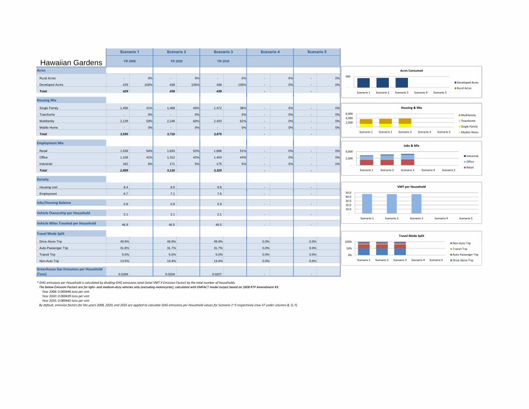
Acres
Rural Acres - 0% - 0% - 0% - 0% - 0%
Developed Acres 429 100% 438 100% 438 100% - 0% - 0%
Total 429 438 438 - -
Hawaiian Gardens
Scenario 5Scenario 1 Scenario 2 Scenario 3 Scenario 4
YR 2008 YR 2020 YR 2035
‐
500
Scenario 1 Scenario 2 Scenario 3 Scenario 4 Scenario 5
Acres Consumed
Developed Acres
Rural Acres
Housing Mix
Single Family 1,456 41% 1,468 40% 1,472 38% - 0% - 0%
Townhome - 0% - 0% - 0% - 0% - 0%
Multifamily 2,139 59% 2,248 60% 2,403 62% - 0% - 0%
Mobile Home - 0% - 0% - 0% - 0% - 0%
Total 3,595 3,716 3,875 - -
Employment Mix
‐
500
Scenario 1 Scenario 2 Scenario 3 Scenario 4 Scenario 5
Acres Consumed
Developed Acres
Rural Acres
‐
2,000
4,000
6,000
Scenario 1 Scenario 2 Scenario 3 Scenario 4 Scenario 5
Housing & Mix
Multifamily
Townhome
Single Family
Mobile Home
Jobs & MixEmployment Mix
Retail 1,539 54% 1,633 52% 1,696 51% - 0% - 0%
Office 1,158 41% 1,312 42% 1,454 44% - 0% - 0%
Industrial 162 6% 171 5% 175 5% - 0% - 0%
Total 2,859 3,116 3,325 - -
Density
Housing Unit 8.4 8.5 8.8 - -
‐
500
Scenario 1 Scenario 2 Scenario 3 Scenario 4 Scenario 5
Acres Consumed
Developed Acres
Rural Acres
‐
2,000
4,000
6,000
Scenario 1 Scenario 2 Scenario 3 Scenario 4 Scenario 5
Housing & Mix
Multifamily
Townhome
Single Family
Mobile Home
‐
2,000
4,000
Scenario 1 Scenario 2 Scenario 3 Scenario 4 Scenario 5
Jobs & Mix
Industrial
Office
Retail
50.0
VMT per Household
Employment 6.7 7.1 7.6 - -
Jobs/Housing Balance 0.8 0.8 0.9 - -
Vehicle Ownership per Household 2.1 2.1 2.1 - -
Vehicle Miles Traveled per Household 46.8 46.5 46.5 - -
Travel Mode Split
‐
500
Scenario 1 Scenario 2 Scenario 3 Scenario 4 Scenario 5
Acres Consumed
Developed Acres
Rural Acres
‐
2,000
4,000
6,000
Scenario 1 Scenario 2 Scenario 3 Scenario 4 Scenario 5
Housing & Mix
Multifamily
Townhome
Single Family
Mobile Home
‐
2,000
4,000
Scenario 1 Scenario 2 Scenario 3 Scenario 4 Scenario 5
Jobs & Mix
Industrial
Office
Retail
‐
10.0
20.0
30.0
40.0
50.0
Scenario 1 Scenario 2 Scenario 3 Scenario 4 Scenario 5
VMT per Household
100%
Travel Mode Split
Non Auto TripDrive Alone Trip 49.9% 49.9% 49.9% 0.0% 0.0%
Auto-Passenger Trip 31.6% 31.7% 31.7% 0.0% 0.0%
Transit Trip 5.0% 5.0% 5.0% 0.0% 0.0%
Non-Auto Trip 13.5% 13.4% 13.4% 0.0% 0.0%
Greenhouse Gas Emissions per Household
(Tons) 0.0209 0.0204 0.0207 - -
* GHG emissions per Household is calculated by dividing GHG emissions total (total VMT X Emission Factor) by the total number of households.
The below Emission Factors are for light‐ and medium‐duty vehicles only (excluding motorcycles) calculated with EMFACT model output based on 2008 RTP Amendment #3:
‐
500
Scenario 1 Scenario 2 Scenario 3 Scenario 4 Scenario 5
Acres Consumed
Developed Acres
Rural Acres
‐
2,000
4,000
6,000
Scenario 1 Scenario 2 Scenario 3 Scenario 4 Scenario 5
Housing & Mix
Multifamily
Townhome
Single Family
Mobile Home
‐
2,000
4,000
Scenario 1 Scenario 2 Scenario 3 Scenario 4 Scenario 5
Jobs & Mix
Industrial
Office
Retail
‐
10.0
20.0
30.0
40.0
50.0
Scenario 1 Scenario 2 Scenario 3 Scenario 4 Scenario 5
VMT per Household
0%
50%
100%
Scenario 1 Scenario 2 Scenario 3 Scenario 4 Scenario 5
Travel Mode Split
Non‐Auto Trip
Transit Trip
Auto‐Passenger Trip
Drive Alone Trip
The below Emission Factors are for light‐ and medium‐duty vehicles only (excluding motorcycles), calculated with EMFACT model output based on 2008 RTP Amendment #3:
Year 2008: 0.000446 tons per vmt
Year 2020: 0.000439 tons per vmt
Year 2035: 0.000445 tons per vmt
By default, emission factors for the years 2008, 2020, and 2035 are applied to calculate GHG emissions per Household values for Scenario 1~3 respectively (row 37 under columns B, D, F).
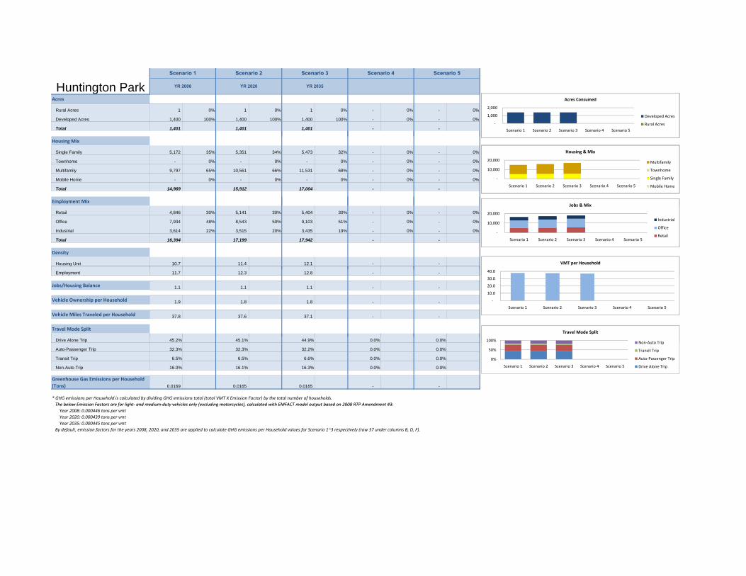
Acres
Rural Acres 1 0% 1 0% 1 0% - 0% - 0%
Developed Acres 1,400 100% 1,400 100% 1,400 100% - 0% - 0%
Total 1,401 1,401 1,401 - -
Huntington ParkScenario 5Scenario 1 Scenario 2 Scenario 3 Scenario 4
YR 2008 YR 2020 YR 2035
‐
1,000
2,000
Scenario 1 Scenario 2 Scenario 3 Scenario 4 Scenario 5
Acres Consumed
Developed Acres
Rural Acres
Housing Mix
Single Family 5,172 35% 5,351 34% 5,473 32% - 0% - 0%
Townhome - 0% - 0% - 0% - 0% - 0%
Multifamily 9,797 65% 10,561 66% 11,531 68% - 0% - 0%
Mobile Home - 0% - 0% - 0% - 0% - 0%
Total 14,969 15,912 17,004 - -
Employment Mix
‐
1,000
2,000
Scenario 1 Scenario 2 Scenario 3 Scenario 4 Scenario 5
Acres Consumed
Developed Acres
Rural Acres
‐
10,000
20,000
Scenario 1 Scenario 2 Scenario 3 Scenario 4 Scenario 5
Housing & Mix
Multifamily
Townhome
Single Family
Mobile Home
Jobs & MixEmployment Mix
Retail 4,846 30% 5,141 30% 5,404 30% - 0% - 0%
Office 7,934 48% 8,543 50% 9,103 51% - 0% - 0%
Industrial 3,614 22% 3,515 20% 3,435 19% - 0% - 0%
Total 16,394 17,199 17,942 - -
Density
Housing Unit 10.7 11.4 12.1 - -
‐
1,000
2,000
Scenario 1 Scenario 2 Scenario 3 Scenario 4 Scenario 5
Acres Consumed
Developed Acres
Rural Acres
‐
10,000
20,000
Scenario 1 Scenario 2 Scenario 3 Scenario 4 Scenario 5
Housing & Mix
Multifamily
Townhome
Single Family
Mobile Home
‐
10,000
20,000
Scenario 1 Scenario 2 Scenario 3 Scenario 4 Scenario 5
Jobs & Mix
Industrial
Office
Retail
40.0
VMT per Household
Employment 11.7 12.3 12.8 - -
Jobs/Housing Balance 1.1 1.1 1.1 - -
Vehicle Ownership per Household 1.9 1.8 1.8 - -
Vehicle Miles Traveled per Household 37.8 37.6 37.1 - -
Travel Mode Split
‐
1,000
2,000
Scenario 1 Scenario 2 Scenario 3 Scenario 4 Scenario 5
Acres Consumed
Developed Acres
Rural Acres
‐
10,000
20,000
Scenario 1 Scenario 2 Scenario 3 Scenario 4 Scenario 5
Housing & Mix
Multifamily
Townhome
Single Family
Mobile Home
‐
10,000
20,000
Scenario 1 Scenario 2 Scenario 3 Scenario 4 Scenario 5
Jobs & Mix
Industrial
Office
Retail
‐
10.0
20.0
30.0
40.0
Scenario 1 Scenario 2 Scenario 3 Scenario 4 Scenario 5
VMT per Household
100%
Travel Mode Split
Non Auto TripDrive Alone Trip 45.2% 45.1% 44.9% 0.0% 0.0%
Auto-Passenger Trip 32.3% 32.3% 32.2% 0.0% 0.0%
Transit Trip 6.5% 6.5% 6.6% 0.0% 0.0%
Non-Auto Trip 16.0% 16.1% 16.3% 0.0% 0.0%
Greenhouse Gas Emissions per Household
(Tons) 0.0169 0.0165 0.0165 - -
* GHG emissions per Household is calculated by dividing GHG emissions total (total VMT X Emission Factor) by the total number of households.
The below Emission Factors are for light‐ and medium‐duty vehicles only (excluding motorcycles) calculated with EMFACT model output based on 2008 RTP Amendment #3:
‐
1,000
2,000
Scenario 1 Scenario 2 Scenario 3 Scenario 4 Scenario 5
Acres Consumed
Developed Acres
Rural Acres
‐
10,000
20,000
Scenario 1 Scenario 2 Scenario 3 Scenario 4 Scenario 5
Housing & Mix
Multifamily
Townhome
Single Family
Mobile Home
‐
10,000
20,000
Scenario 1 Scenario 2 Scenario 3 Scenario 4 Scenario 5
Jobs & Mix
Industrial
Office
Retail
‐
10.0
20.0
30.0
40.0
Scenario 1 Scenario 2 Scenario 3 Scenario 4 Scenario 5
VMT per Household
0%
50%
100%
Scenario 1 Scenario 2 Scenario 3 Scenario 4 Scenario 5
Travel Mode Split
Non‐Auto Trip
Transit Trip
Auto‐Passenger Trip
Drive Alone Trip
The below Emission Factors are for light‐ and medium‐duty vehicles only (excluding motorcycles), calculated with EMFACT model output based on 2008 RTP Amendment #3:
Year 2008: 0.000446 tons per vmt
Year 2020: 0.000439 tons per vmt
Year 2035: 0.000445 tons per vmt
By default, emission factors for the years 2008, 2020, and 2035 are applied to calculate GHG emissions per Household values for Scenario 1~3 respectively (row 37 under columns B, D, F).

Acres
Rural Acres 550 23% 728 27% 728 27% - 0% - 0%
Developed Acres 1,852 77% 1,959 73% 1,959 73% - 0% - 0%
Total 2,402 2,687 2,687 - -
La Habra Heights
Scenario 5Scenario 1 Scenario 2 Scenario 3 Scenario 4
YR 2008 YR 2020 YR 2035
‐
2,000
4,000
Scenario 1 Scenario 2 Scenario 3 Scenario 4 Scenario 5
Acres Consumed
Developed Acres
Rural Acres
Housing Mix
Single Family 1,929 98% 2,052 97% 2,179 94% - 0% - 0%
Townhome - 0% - 0% - 0% - 0% - 0%
Multifamily 32 2% 55 3% 132 6% - 0% - 0%
Mobile Home - 0% - 0% - 0% - 0% - 0%
Total 1,961 2,107 2,311 - -
Employment Mix
‐
2,000
4,000
Scenario 1 Scenario 2 Scenario 3 Scenario 4 Scenario 5
Acres Consumed
Developed Acres
Rural Acres
‐
1,000
2,000
3,000
Scenario 1 Scenario 2 Scenario 3 Scenario 4 Scenario 5
Housing & Mix
Multifamily
Townhome
Single Family
Mobile Home
Jobs & MixEmployment Mix
Retail 173 22% 190 22% 191 21% - 0% - 0%
Office 375 47% 423 49% 468 52% - 0% - 0%
Industrial 244 31% 248 29% 239 27% - 0% - 0%
Total 793 861 898 - -
Density
Housing Unit 0.8 0.8 0.9 - -
‐
2,000
4,000
Scenario 1 Scenario 2 Scenario 3 Scenario 4 Scenario 5
Acres Consumed
Developed Acres
Rural Acres
‐
1,000
2,000
3,000
Scenario 1 Scenario 2 Scenario 3 Scenario 4 Scenario 5
Housing & Mix
Multifamily
Townhome
Single Family
Mobile Home
‐
500
1,000
Scenario 1 Scenario 2 Scenario 3 Scenario 4 Scenario 5
Jobs & Mix
Industrial
Office
Retail
80.0
VMT per Household
Employment 0.3 0.3 0.3 - -
Jobs/Housing Balance 0.4 0.4 0.4 - -
Vehicle Ownership per Household 2.5 2.5 2.5 - -
Vehicle Miles Traveled per Household 60.6 60.6 60.6 - -
Travel Mode Split
‐
2,000
4,000
Scenario 1 Scenario 2 Scenario 3 Scenario 4 Scenario 5
Acres Consumed
Developed Acres
Rural Acres
‐
1,000
2,000
3,000
Scenario 1 Scenario 2 Scenario 3 Scenario 4 Scenario 5
Housing & Mix
Multifamily
Townhome
Single Family
Mobile Home
‐
500
1,000
Scenario 1 Scenario 2 Scenario 3 Scenario 4 Scenario 5
Jobs & Mix
Industrial
Office
Retail
‐
20.0
40.0
60.0
80.0
Scenario 1 Scenario 2 Scenario 3 Scenario 4 Scenario 5
VMT per Household
100%
Travel Mode Split
Non Auto TripDrive Alone Trip 69.9% 69.9% 69.8% 0.0% 0.0%
Auto-Passenger Trip 26.6% 26.6% 26.6% 0.0% 0.0%
Transit Trip 2.1% 2.1% 2.2% 0.0% 0.0%
Non-Auto Trip 1.4% 1.4% 1.5% 0.0% 0.0%
Greenhouse Gas Emissions per Household
(Tons) 0.0270 0.0266 0.0270 - -
* GHG emissions per Household is calculated by dividing GHG emissions total (total VMT X Emission Factor) by the total number of households.
The below Emission Factors are for light‐ and medium‐duty vehicles only (excluding motorcycles) calculated with EMFACT model output based on 2008 RTP Amendment #3:
‐
2,000
4,000
Scenario 1 Scenario 2 Scenario 3 Scenario 4 Scenario 5
Acres Consumed
Developed Acres
Rural Acres
‐
1,000
2,000
3,000
Scenario 1 Scenario 2 Scenario 3 Scenario 4 Scenario 5
Housing & Mix
Multifamily
Townhome
Single Family
Mobile Home
‐
500
1,000
Scenario 1 Scenario 2 Scenario 3 Scenario 4 Scenario 5
Jobs & Mix
Industrial
Office
Retail
‐
20.0
40.0
60.0
80.0
Scenario 1 Scenario 2 Scenario 3 Scenario 4 Scenario 5
VMT per Household
0%
50%
100%
Scenario 1 Scenario 2 Scenario 3 Scenario 4 Scenario 5
Travel Mode Split
Non‐Auto Trip
Transit Trip
Auto‐Passenger Trip
Drive Alone Trip
The below Emission Factors are for light‐ and medium‐duty vehicles only (excluding motorcycles), calculated with EMFACT model output based on 2008 RTP Amendment #3:
Year 2008: 0.000446 tons per vmt
Year 2020: 0.000439 tons per vmt
Year 2035: 0.000445 tons per vmt
By default, emission factors for the years 2008, 2020, and 2035 are applied to calculate GHG emissions per Household values for Scenario 1~3 respectively (row 37 under columns B, D, F).
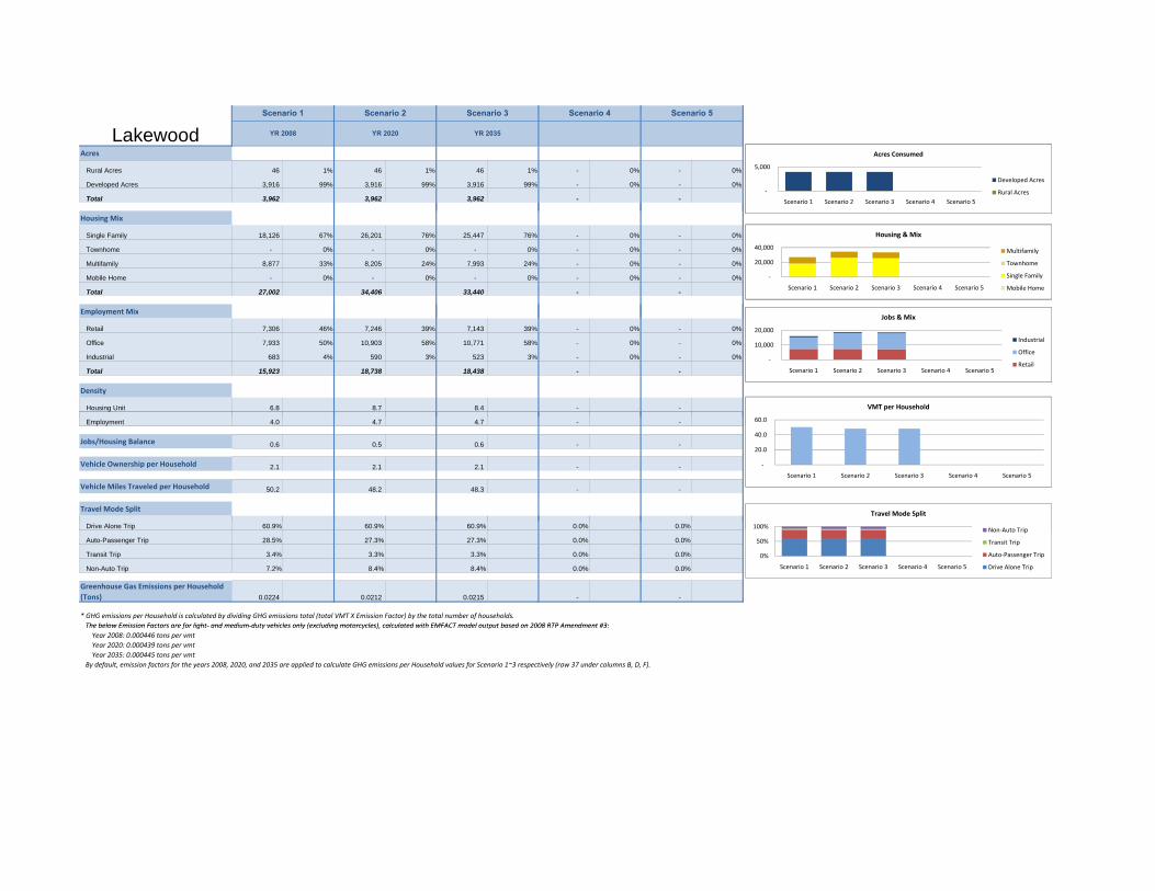
Acres
Rural Acres 46 1% 46 1% 46 1% - 0% - 0%
Developed Acres 3,916 99% 3,916 99% 3,916 99% - 0% - 0%
Total 3,962 3,962 3,962 - -
LakewoodScenario 5Scenario 1 Scenario 2 Scenario 3 Scenario 4
YR 2008 YR 2020 YR 2035
‐
5,000
Scenario 1 Scenario 2 Scenario 3 Scenario 4 Scenario 5
Acres Consumed
Developed Acres
Rural Acres
Housing Mix
Single Family 18,126 67% 26,201 76% 25,447 76% - 0% - 0%
Townhome - 0% - 0% - 0% - 0% - 0%
Multifamily 8,877 33% 8,205 24% 7,993 24% - 0% - 0%
Mobile Home - 0% - 0% - 0% - 0% - 0%
Total 27,002 34,406 33,440 - -
Employment Mix
‐
5,000
Scenario 1 Scenario 2 Scenario 3 Scenario 4 Scenario 5
Acres Consumed
Developed Acres
Rural Acres
‐
20,000
40,000
Scenario 1 Scenario 2 Scenario 3 Scenario 4 Scenario 5
Housing & Mix
Multifamily
Townhome
Single Family
Mobile Home
Jobs & MixEmployment Mix
Retail 7,306 46% 7,246 39% 7,143 39% - 0% - 0%
Office 7,933 50% 10,903 58% 10,771 58% - 0% - 0%
Industrial 683 4% 590 3% 523 3% - 0% - 0%
Total 15,923 18,738 18,438 - -
Density
Housing Unit 6.8 8.7 8.4 - -
‐
5,000
Scenario 1 Scenario 2 Scenario 3 Scenario 4 Scenario 5
Acres Consumed
Developed Acres
Rural Acres
‐
20,000
40,000
Scenario 1 Scenario 2 Scenario 3 Scenario 4 Scenario 5
Housing & Mix
Multifamily
Townhome
Single Family
Mobile Home
‐
10,000
20,000
Scenario 1 Scenario 2 Scenario 3 Scenario 4 Scenario 5
Jobs & Mix
Industrial
Office
Retail
60.0
VMT per Household
Employment 4.0 4.7 4.7 - -
Jobs/Housing Balance 0.6 0.5 0.6 - -
Vehicle Ownership per Household 2.1 2.1 2.1 - -
Vehicle Miles Traveled per Household 50.2 48.2 48.3 - -
Travel Mode Split
‐
5,000
Scenario 1 Scenario 2 Scenario 3 Scenario 4 Scenario 5
Acres Consumed
Developed Acres
Rural Acres
‐
20,000
40,000
Scenario 1 Scenario 2 Scenario 3 Scenario 4 Scenario 5
Housing & Mix
Multifamily
Townhome
Single Family
Mobile Home
‐
10,000
20,000
Scenario 1 Scenario 2 Scenario 3 Scenario 4 Scenario 5
Jobs & Mix
Industrial
Office
Retail
‐
20.0
40.0
60.0
Scenario 1 Scenario 2 Scenario 3 Scenario 4 Scenario 5
VMT per Household
100%
Travel Mode Split
Non Auto TripDrive Alone Trip 60.9% 60.9% 60.9% 0.0% 0.0%
Auto-Passenger Trip 28.5% 27.3% 27.3% 0.0% 0.0%
Transit Trip 3.4% 3.3% 3.3% 0.0% 0.0%
Non-Auto Trip 7.2% 8.4% 8.4% 0.0% 0.0%
Greenhouse Gas Emissions per Household
(Tons) 0.0224 0.0212 0.0215 - -
* GHG emissions per Household is calculated by dividing GHG emissions total (total VMT X Emission Factor) by the total number of households.
The below Emission Factors are for light‐ and medium‐duty vehicles only (excluding motorcycles) calculated with EMFACT model output based on 2008 RTP Amendment #3:
‐
5,000
Scenario 1 Scenario 2 Scenario 3 Scenario 4 Scenario 5
Acres Consumed
Developed Acres
Rural Acres
‐
20,000
40,000
Scenario 1 Scenario 2 Scenario 3 Scenario 4 Scenario 5
Housing & Mix
Multifamily
Townhome
Single Family
Mobile Home
‐
10,000
20,000
Scenario 1 Scenario 2 Scenario 3 Scenario 4 Scenario 5
Jobs & Mix
Industrial
Office
Retail
‐
20.0
40.0
60.0
Scenario 1 Scenario 2 Scenario 3 Scenario 4 Scenario 5
VMT per Household
0%
50%
100%
Scenario 1 Scenario 2 Scenario 3 Scenario 4 Scenario 5
Travel Mode Split
Non‐Auto Trip
Transit Trip
Auto‐Passenger Trip
Drive Alone Trip
The below Emission Factors are for light‐ and medium‐duty vehicles only (excluding motorcycles), calculated with EMFACT model output based on 2008 RTP Amendment #3:
Year 2008: 0.000446 tons per vmt
Year 2020: 0.000439 tons per vmt
Year 2035: 0.000445 tons per vmt
By default, emission factors for the years 2008, 2020, and 2035 are applied to calculate GHG emissions per Household values for Scenario 1~3 respectively (row 37 under columns B, D, F).

Acres
Rural Acres 24 1% 43 1% 43 1% - 0% - 0%
Developed Acres 3,460 99% 3,555 99% 3,555 99% - 0% - 0%
Total 3,484 3,597 3,597 - -
La MiradaScenario 5Scenario 1 Scenario 2 Scenario 3 Scenario 4
YR 2008 YR 2020 YR 2035
‐
2,000
4,000
Scenario 1 Scenario 2 Scenario 3 Scenario 4 Scenario 5
Acres Consumed
Developed Acres
Rural Acres
Housing Mix
Single Family 11,939 81% 12,049 80% 12,049 78% - 0% - 0%
Townhome - 0% - 0% - 0% - 0% - 0%
Multifamily 2,781 19% 2,958 20% 3,317 22% - 0% - 0%
Mobile Home - 0% - 0% - 0% - 0% - 0%
Total 14,720 15,007 15,366 - -
Employment Mix
‐
2,000
4,000
Scenario 1 Scenario 2 Scenario 3 Scenario 4 Scenario 5
Acres Consumed
Developed Acres
Rural Acres
‐
10,000
20,000
Scenario 1 Scenario 2 Scenario 3 Scenario 4 Scenario 5
Housing & Mix
Multifamily
Townhome
Single Family
Mobile Home
Jobs & MixEmployment Mix
Retail 4,588 24% 4,789 24% 4,955 24% - 0% - 0%
Office 8,690 45% 9,076 46% 9,470 47% - 0% - 0%
Industrial 6,070 31% 5,973 30% 5,929 29% - 0% - 0%
Total 19,348 19,838 20,354 - -
Density
Housing Unit 4.2 4.2 4.3 - -
‐
2,000
4,000
Scenario 1 Scenario 2 Scenario 3 Scenario 4 Scenario 5
Acres Consumed
Developed Acres
Rural Acres
‐
10,000
20,000
Scenario 1 Scenario 2 Scenario 3 Scenario 4 Scenario 5
Housing & Mix
Multifamily
Townhome
Single Family
Mobile Home
‐
10,000
20,000
30,000
Scenario 1 Scenario 2 Scenario 3 Scenario 4 Scenario 5
Jobs & Mix
Industrial
Office
Retail
60.0
VMT per Household
Employment 5.6 5.5 5.7 - -
Jobs/Housing Balance 1.3 1.3 1.3 - -
Vehicle Ownership per Household 2.2 2.2 2.2 - -
Vehicle Miles Traveled per Household 50.5 50.4 50.2 - -
Travel Mode Split
‐
2,000
4,000
Scenario 1 Scenario 2 Scenario 3 Scenario 4 Scenario 5
Acres Consumed
Developed Acres
Rural Acres
‐
10,000
20,000
Scenario 1 Scenario 2 Scenario 3 Scenario 4 Scenario 5
Housing & Mix
Multifamily
Townhome
Single Family
Mobile Home
‐
10,000
20,000
30,000
Scenario 1 Scenario 2 Scenario 3 Scenario 4 Scenario 5
Jobs & Mix
Industrial
Office
Retail
‐
20.0
40.0
60.0
Scenario 1 Scenario 2 Scenario 3 Scenario 4 Scenario 5
VMT per Household
100%
Travel Mode Split
Non Auto TripDrive Alone Trip 61.5% 61.6% 61.5% 0.0% 0.0%
Auto-Passenger Trip 27.7% 27.7% 27.7% 0.0% 0.0%
Transit Trip 3.1% 3.1% 3.1% 0.0% 0.0%
Non-Auto Trip 7.6% 7.6% 7.7% 0.0% 0.0%
Greenhouse Gas Emissions per Household
(Tons) 0.0225 0.0221 0.0224 - -
* GHG emissions per Household is calculated by dividing GHG emissions total (total VMT X Emission Factor) by the total number of households.
The below Emission Factors are for light‐ and medium‐duty vehicles only (excluding motorcycles) calculated with EMFACT model output based on 2008 RTP Amendment #3:
‐
2,000
4,000
Scenario 1 Scenario 2 Scenario 3 Scenario 4 Scenario 5
Acres Consumed
Developed Acres
Rural Acres
‐
10,000
20,000
Scenario 1 Scenario 2 Scenario 3 Scenario 4 Scenario 5
Housing & Mix
Multifamily
Townhome
Single Family
Mobile Home
‐
10,000
20,000
30,000
Scenario 1 Scenario 2 Scenario 3 Scenario 4 Scenario 5
Jobs & Mix
Industrial
Office
Retail
‐
20.0
40.0
60.0
Scenario 1 Scenario 2 Scenario 3 Scenario 4 Scenario 5
VMT per Household
0%
50%
100%
Scenario 1 Scenario 2 Scenario 3 Scenario 4 Scenario 5
Travel Mode Split
Non‐Auto Trip
Transit Trip
Auto‐Passenger Trip
Drive Alone Trip
The below Emission Factors are for light‐ and medium‐duty vehicles only (excluding motorcycles), calculated with EMFACT model output based on 2008 RTP Amendment #3:
Year 2008: 0.000446 tons per vmt
Year 2020: 0.000439 tons per vmt
Year 2035: 0.000445 tons per vmt
By default, emission factors for the years 2008, 2020, and 2035 are applied to calculate GHG emissions per Household values for Scenario 1~3 respectively (row 37 under columns B, D, F).

Long BeachAcres
Vacant Acres - 0% 72.28 0% 94.52 0% 383.64 2% 1,829.24 8%Developed Acres 21,817.48 100% 21,817.48 100% 21,817.48 100% 21,817.48 98% 21,817.48 92%
Housing MixSingle Family 65,205.95 33% 64,883.34 33% 65,192.71 33% 65,176.48 33% 51,111.87 6%Townhome - 0% - 0% - 0% - 0% - 0%Multifamily 134,973.33 67% 134,278.61 67% 134,041.02 67% 134,028.72 67% 803,273.02 94%Mobile Home - 0% - 0% - 0% - 0% - 0%
200,179.29 199,161.95 199,233.72 199,205.20 854,384.89 Employment Mix
Retail 39,535.31 12% 43,895.43 12% 47,473.53 12% 49,121.46 11% 600,486.35 18%Office 281,561.65 85% 316,292.88 86% 338,726.51 86% 385,642.69 87% 2,814,008.83 82%Industrial 9,303.69 3% 9,048.60 2% 8,947.61 2% 10,748.37 2% 8,004.07 0%
330,400.65 369,236.92 395,147.65 445,512.52 3,422,499.25 Density
Housing Unit 9.18 9.10 9.09 8.97 36.13 Employment 15.14 16.87 18.03 20.07 144.73
Jobs/Housing Balance 1.65 1.85 1.98 2.24 4.01
Vehicle Ownership per Household 1.57 1.57 1.57 1.57 1.40
Vehicle Miles Traveled per Household 32.77 32.01 32.01 32.01 27.12
Travel Mode SplitDrive Alone Trip 54.2% 54.2% 54.3% 54.3% 49.5%Auto-Passenger Trip 26.8% 26.9% 26.9% 26.9% 26.0%Transit Trip 4.9% 4.7% 4.7% 4.7% 5.3%Non-Auto Trip 14.1% 14.1% 14.1% 14.1% 19.2%
Greenhouse Gas Emissions (Tons/Day) 3,201.33 3,110.83 3,112.10 3,111.68 11,308.26 Greenhouse Gas Emissions (Tons/Household) 0.01599229374 0.01561958158 0.01562037241 0.01562047180 0.01323556088
2008 Total Population 491273.002008 Total Household 166363.002008 Average Household Size 2.95
GHG per Capita 0.0054 0.0053 0.0053 0.0053 0.0045
*Based on April 4 discussion with Ira Brown, the Scenarios are defined as above (2008, 2020 and 2035)
Scenario 5Scenario 1 (2008) Scenario 2 Scenario 3 (2020) Scenario 4 (2035)
- 72.28 94.52 383.64 1,829.24
21,817.48 21,817.48 21,817.48 21,817.48 21,817.48
-
5,000
10,000
15,000
20,000
25,000
Scenario 1 (2008)
Scenario 2 Scenario 3 (2020)
Scenario 4 (2035)
Scenario 5
Acres Developed Acres
Vacant Acres
65,205.95 64,883.34 65,192.71 65,176.48 51,111.87 - - - - -
134,973.33 134,278.61 134,041.02 134,028.72
803,273.02
-
100,000
200,000
300,000
400,000
500,000
600,000
700,000
800,000
900,000
Scenario 1 (2008)Scenario 2Scenario 3 (2020)Scenario 4 (2035)Scenario 5
Housing Mix Multifamily
Townhome
Single Family
39,535.31 43,895.43 47,473.53 49,121.46 600,486.35
281,561.65 316,292.88 338,726.51 385,642.69
2,814,008.83
9,303.69 9,048.60 8,947.61 10,748.37
8,004.07
-
500,000
1,000,000
1,500,000
2,000,000
2,500,000
3,000,000
3,500,000
4,000,000
Scenario 1 (2008)
Scenario 2 Scenario 3 (2020)
Scenario 4 (2035)
Scenario 5
Employment Mix Industrial Office
Retail
1.65 1.85
1.98 2.24
-
0.50
1.00
1.50
2.00
2.50
3.00
Scenario 1 (2008) Scenario 2 Scenario 3 (2020)Scenario 4 (2035) Scenario 5
Jobs Housing Balance

Acres
Rural Acres 3 0% 7 0% 7 0% - 0% - 0%
Developed Acres 2,124 100% 2,185 100% 2,185 100% - 0% - 0%
Total 2,127 2,191 2,191 - -
LynwoodScenario 5Scenario 1 Scenario 2 Scenario 3 Scenario 4
YR 2008 YR 2020 YR 2035
‐
2,000
4,000
Scenario 1 Scenario 2 Scenario 3 Scenario 4 Scenario 5
Acres Consumed
Developed Acres
Rural Acres
Housing Mix
Single Family 7,803 49% 7,973 48% 7,973 47% - 0% - 0%
Townhome - 0% - 0% - 0% - 0% - 0%
Multifamily 7,974 51% 8,564 52% 8,839 53% - 0% - 0%
Mobile Home - 0% - 0% - 0% - 0% - 0%
Total 15,776 16,538 16,812 - -
Employment Mix
‐
2,000
4,000
Scenario 1 Scenario 2 Scenario 3 Scenario 4 Scenario 5
Acres Consumed
Developed Acres
Rural Acres
‐
10,000
20,000
Scenario 1 Scenario 2 Scenario 3 Scenario 4 Scenario 5
Housing & Mix
Multifamily
Townhome
Single Family
Mobile Home
Jobs & MixEmployment Mix
Retail 2,742 22% 4,041 29% 5,564 36% - 0% - 0%
Office 6,770 54% 7,141 51% 7,740 50% - 0% - 0%
Industrial 3,081 24% 2,862 20% 2,227 14% - 0% - 0%
Total 12,593 14,044 15,531 - -
Density
Housing Unit 7.4 7.5 7.7 - -
‐
2,000
4,000
Scenario 1 Scenario 2 Scenario 3 Scenario 4 Scenario 5
Acres Consumed
Developed Acres
Rural Acres
‐
10,000
20,000
Scenario 1 Scenario 2 Scenario 3 Scenario 4 Scenario 5
Housing & Mix
Multifamily
Townhome
Single Family
Mobile Home
‐
10,000
20,000
Scenario 1 Scenario 2 Scenario 3 Scenario 4 Scenario 5
Jobs & Mix
Industrial
Office
Retail
50.0
VMT per Household
Employment 5.9 6.4 7.1 - -
Jobs/Housing Balance 0.8 0.8 0.9 - -
Vehicle Ownership per Household 2.2 2.2 2.2 - -
Vehicle Miles Traveled per Household 46.8 46.6 46.5 - -
Travel Mode Split
‐
2,000
4,000
Scenario 1 Scenario 2 Scenario 3 Scenario 4 Scenario 5
Acres Consumed
Developed Acres
Rural Acres
‐
10,000
20,000
Scenario 1 Scenario 2 Scenario 3 Scenario 4 Scenario 5
Housing & Mix
Multifamily
Townhome
Single Family
Mobile Home
‐
10,000
20,000
Scenario 1 Scenario 2 Scenario 3 Scenario 4 Scenario 5
Jobs & Mix
Industrial
Office
Retail
‐
10.0
20.0
30.0
40.0
50.0
Scenario 1 Scenario 2 Scenario 3 Scenario 4 Scenario 5
VMT per Household
100%
Travel Mode Split
Non Auto TripDrive Alone Trip 46.5% 46.5% 46.5% 0.0% 0.0%
Auto-Passenger Trip 33.9% 33.9% 33.9% 0.0% 0.0%
Transit Trip 5.4% 5.4% 5.4% 0.0% 0.0%
Non-Auto Trip 14.2% 14.2% 14.2% 0.0% 0.0%
Greenhouse Gas Emissions per Household
(Tons) 0.0209 0.0204 0.0207 - -
* GHG emissions per Household is calculated by dividing GHG emissions total (total VMT X Emission Factor) by the total number of households.
The below Emission Factors are for light‐ and medium‐duty vehicles only (excluding motorcycles) calculated with EMFACT model output based on 2008 RTP Amendment #3:
‐
2,000
4,000
Scenario 1 Scenario 2 Scenario 3 Scenario 4 Scenario 5
Acres Consumed
Developed Acres
Rural Acres
‐
10,000
20,000
Scenario 1 Scenario 2 Scenario 3 Scenario 4 Scenario 5
Housing & Mix
Multifamily
Townhome
Single Family
Mobile Home
‐
10,000
20,000
Scenario 1 Scenario 2 Scenario 3 Scenario 4 Scenario 5
Jobs & Mix
Industrial
Office
Retail
‐
10.0
20.0
30.0
40.0
50.0
Scenario 1 Scenario 2 Scenario 3 Scenario 4 Scenario 5
VMT per Household
0%
50%
100%
Scenario 1 Scenario 2 Scenario 3 Scenario 4 Scenario 5
Travel Mode Split
Non‐Auto Trip
Transit Trip
Auto‐Passenger Trip
Drive Alone Trip
The below Emission Factors are for light‐ and medium‐duty vehicles only (excluding motorcycles), calculated with EMFACT model output based on 2008 RTP Amendment #3:
Year 2008: 0.000446 tons per vmt
Year 2020: 0.000439 tons per vmt
Year 2035: 0.000445 tons per vmt
By default, emission factors for the years 2008, 2020, and 2035 are applied to calculate GHG emissions per Household values for Scenario 1~3 respectively (row 37 under columns B, D, F).

Acres
Rural Acres 3 1% 3 1% 3 1% - 0% - 0%
Developed Acres 556 99% 556 99% 556 99% - 0% - 0%
Total 559 559 559 - -
MaywoodScenario 5Scenario 1 Scenario 2 Scenario 3 Scenario 4
YR 2008 YR 2020 YR 2035
‐
500
1,000
Scenario 1 Scenario 2 Scenario 3 Scenario 4 Scenario 5
Acres Consumed
Developed Acres
Rural Acres
Housing Mix
Single Family 2,730 41% 2,730 41% 2,730 40% - 0% - 0%
Townhome - 0% - 0% - 0% - 0% - 0%
Multifamily 3,864 59% 3,931 59% 4,013 60% - 0% - 0%
Mobile Home - 0% - 0% - 0% - 0% - 0%
Total 6,594 6,661 6,743 - -
Employment Mix
‐
500
1,000
Scenario 1 Scenario 2 Scenario 3 Scenario 4 Scenario 5
Acres Consumed
Developed Acres
Rural Acres
‐
5,000
10,000
Scenario 1 Scenario 2 Scenario 3 Scenario 4 Scenario 5
Housing & Mix
Multifamily
Townhome
Single Family
Mobile Home
Jobs & MixEmployment Mix
Retail 1,108 29% 1,194 29% 1,254 30% - 0% - 0%
Office 1,832 47% 1,964 48% 2,079 49% - 0% - 0%
Industrial 921 24% 903 22% 885 21% - 0% - 0%
Total 3,861 4,060 4,218 - -
Density
Housing Unit 11.8 11.9 12.1 - -
‐
500
1,000
Scenario 1 Scenario 2 Scenario 3 Scenario 4 Scenario 5
Acres Consumed
Developed Acres
Rural Acres
‐
5,000
10,000
Scenario 1 Scenario 2 Scenario 3 Scenario 4 Scenario 5
Housing & Mix
Multifamily
Townhome
Single Family
Mobile Home
‐
2,000
4,000
6,000
Scenario 1 Scenario 2 Scenario 3 Scenario 4 Scenario 5
Jobs & Mix
Industrial
Office
Retail
50.0
VMT per Household
Employment 6.9 7.3 7.5 - -
Jobs/Housing Balance 0.6 0.6 0.6 - -
Vehicle Ownership per Household 2.0 2.0 2.0 - -
Vehicle Miles Traveled per Household 43.0 42.9 42.9 - -
Travel Mode Split
‐
500
1,000
Scenario 1 Scenario 2 Scenario 3 Scenario 4 Scenario 5
Acres Consumed
Developed Acres
Rural Acres
‐
5,000
10,000
Scenario 1 Scenario 2 Scenario 3 Scenario 4 Scenario 5
Housing & Mix
Multifamily
Townhome
Single Family
Mobile Home
‐
2,000
4,000
6,000
Scenario 1 Scenario 2 Scenario 3 Scenario 4 Scenario 5
Jobs & Mix
Industrial
Office
Retail
‐
10.0
20.0
30.0
40.0
50.0
Scenario 1 Scenario 2 Scenario 3 Scenario 4 Scenario 5
VMT per Household
100%
Travel Mode Split
Non Auto TripDrive Alone Trip 45.9% 45.9% 45.9% 0.0% 0.0%
Auto-Passenger Trip 32.9% 32.9% 32.9% 0.0% 0.0%
Transit Trip 6.1% 6.1% 6.1% 0.0% 0.0%
Non-Auto Trip 15.1% 15.1% 15.1% 0.0% 0.0%
Greenhouse Gas Emissions per Household
(Tons) 0.0192 0.0189 0.0191 - -
* GHG emissions per Household is calculated by dividing GHG emissions total (total VMT X Emission Factor) by the total number of households.
The below Emission Factors are for light‐ and medium‐duty vehicles only (excluding motorcycles) calculated with EMFACT model output based on 2008 RTP Amendment #3:
‐
500
1,000
Scenario 1 Scenario 2 Scenario 3 Scenario 4 Scenario 5
Acres Consumed
Developed Acres
Rural Acres
‐
5,000
10,000
Scenario 1 Scenario 2 Scenario 3 Scenario 4 Scenario 5
Housing & Mix
Multifamily
Townhome
Single Family
Mobile Home
‐
2,000
4,000
6,000
Scenario 1 Scenario 2 Scenario 3 Scenario 4 Scenario 5
Jobs & Mix
Industrial
Office
Retail
‐
10.0
20.0
30.0
40.0
50.0
Scenario 1 Scenario 2 Scenario 3 Scenario 4 Scenario 5
VMT per Household
0%
50%
100%
Scenario 1 Scenario 2 Scenario 3 Scenario 4 Scenario 5
Travel Mode Split
Non‐Auto Trip
Transit Trip
Auto‐Passenger Trip
Drive Alone Trip
The below Emission Factors are for light‐ and medium‐duty vehicles only (excluding motorcycles), calculated with EMFACT model output based on 2008 RTP Amendment #3:
Year 2008: 0.000446 tons per vmt
Year 2020: 0.000439 tons per vmt
Year 2035: 0.000445 tons per vmt
By default, emission factors for the years 2008, 2020, and 2035 are applied to calculate GHG emissions per Household values for Scenario 1~3 respectively (row 37 under columns B, D, F).

Acres
Rural Acres 24 1% 28 1% 28 1% 24 1% - 0%
Developed Acres 4,086 99% 4,087 99% 4,063 99% 3,460 99% - 0%
Total 4,110 4,115 4,091 3,484 -
blank blankNorwalkScenario 5Scenario 1 Scenario 2 Scenario 3 Scenario 4
YR 2008 YR 2020 YR 2035
‐
5,000
Scenario 1 Scenario 2 Scenario 3 Scenario 4 Scenario 5
Acres Consumed
Developed Acres
Rural Acres
Housing Mix
Single Family 20,297 70% 20,297 70% 20,286 70% 11,939 81% - 0%
Townhome - 0% - 0% - 0% - 0% - 0%
Multifamily 8,196 28% 8,196 28% 8,194 28% 2,781 19% - 0%
Mobile Home 423 1% 423 1% 423 1% - 0% - 0%
Total 28,494 28,494 28,481 14,720 -
Employment Mix
‐
5,000
Scenario 1 Scenario 2 Scenario 3 Scenario 4 Scenario 5
Acres Consumed
Developed Acres
Rural Acres
‐
20,000
40,000
Scenario 1 Scenario 2 Scenario 3 Scenario 4 Scenario 5
Housing & MixMultifamily
Townhome
Single Family
Mobile Home
Jobs & MixEmployment Mix
Retail 6,339 25% 6,342 25% 6,350 26% 4,588 24% - 0%
Office 15,154 61% 15,251 61% 15,277 61% 8,690 45% - 0%
Industrial 3,375 14% 3,375 14% 3,244 13% 6,070 31% - 0%
Total 24,868 24,969 24,871 19,348 -
Density
Housing Unit 7.0 7.0 7.1 4.2 -
‐
5,000
Scenario 1 Scenario 2 Scenario 3 Scenario 4 Scenario 5
Acres Consumed
Developed Acres
Rural Acres
‐
20,000
40,000
Scenario 1 Scenario 2 Scenario 3 Scenario 4 Scenario 5
Housing & MixMultifamily
Townhome
Single Family
Mobile Home
‐
10,000
20,000
30,000
Scenario 1 Scenario 2 Scenario 3 Scenario 4 Scenario 5
Jobs & Mix
Industrial
Office
Retail
60.0
VMT per Household
Employment 6.1 6.1 6.1 5.6 -
Jobs/Housing Balance 0.9 0.9 0.9 1.3 -
Vehicle Ownership per Household 2.2 2.2 2.2 2.2 -
Vehicle Miles Traveled per Household 48.5 48.6 48.5 50.5 -
Travel Mode Split
‐
5,000
Scenario 1 Scenario 2 Scenario 3 Scenario 4 Scenario 5
Acres Consumed
Developed Acres
Rural Acres
‐
20,000
40,000
Scenario 1 Scenario 2 Scenario 3 Scenario 4 Scenario 5
Housing & MixMultifamily
Townhome
Single Family
Mobile Home
‐
10,000
20,000
30,000
Scenario 1 Scenario 2 Scenario 3 Scenario 4 Scenario 5
Jobs & Mix
Industrial
Office
Retail
‐
20.0
40.0
60.0
Scenario 1 Scenario 2 Scenario 3 Scenario 4 Scenario 5
VMT per Household
100%
Travel Mode SplitNon‐Auto Trip
Drive Alone Trip 54.2% 54.2% 54.2% 61.5% 0.0%
Auto-Passenger Trip 30.5% 30.5% 30.5% 27.7% 0.0%
Transit Trip 4.3% 4.3% 4.3% 3.1% 0.0%
Non-Auto Trip 11.0% 11.0% 11.0% 7.6% 0.0%
Greenhouse Gas Emissions per Household
(Tons) 0.0216 0.0213 0.0216 0.0225 -
* GHG emissions per Household is calculated by dividing GHG emissions total (total VMT X Emission Factor) by the total number of households.
The below Emission Factors are for light‐ and medium‐duty vehicles only (excluding motorcycles) calculated with EMFACT model output based on 2008 RTP Amendment #3:
‐
5,000
Scenario 1 Scenario 2 Scenario 3 Scenario 4 Scenario 5
Acres Consumed
Developed Acres
Rural Acres
‐
20,000
40,000
Scenario 1 Scenario 2 Scenario 3 Scenario 4 Scenario 5
Housing & MixMultifamily
Townhome
Single Family
Mobile Home
‐
10,000
20,000
30,000
Scenario 1 Scenario 2 Scenario 3 Scenario 4 Scenario 5
Jobs & Mix
Industrial
Office
Retail
‐
20.0
40.0
60.0
Scenario 1 Scenario 2 Scenario 3 Scenario 4 Scenario 5
VMT per Household
0%
50%
100%
Scenario 1 Scenario 2 Scenario 3 Scenario 4 Scenario 5
Travel Mode SplitNon‐Auto Trip
Transit Trip
Auto‐Passenger Trip
Drive Alone Trip
The below Emission Factors are for light‐ and medium‐duty vehicles only (excluding motorcycles), calculated with EMFACT model output based on 2008 RTP Amendment #3:
Year 2008: 0.000446 tons per vmt
Year 2020: 0.000439 tons per vmt
Year 2035: 0.000445 tons per vmt
By default, emission factors for the years 2008, 2020, and 2035 are applied to calculate GHG emissions per Household values for Scenario 1~3 respectively (row 37 under columns B, D, F).

Acres
Rural Acres 68 3% 73 4% 73 4% - 0% - 0%
Developed Acres 1,951 97% 1,970 96% 1,970 96% - 0% - 0%
Total 2,019 2,043 2,043 - -
ParamountScenario 5Scenario 1 Scenario 2 Scenario 3 Scenario 4
YR 2008 YR 2020 YR 2035
‐
2,000
4,000
Scenario 1 Scenario 2 Scenario 3 Scenario 4 Scenario 5
Acres Consumed
Developed Acres
Rural Acres
Housing Mix
Single Family 5,972 43% 6,000 42% 6,000 41% - 0% - 0%
Townhome - 0% - 0% - 0% - 0% - 0%
Multifamily 8,004 57% 8,156 58% 8,532 59% - 0% - 0%
Mobile Home - 0% - 0% - 0% - 0% - 0%
Total 13,976 14,156 14,532 - -
Employment Mix
‐
2,000
4,000
Scenario 1 Scenario 2 Scenario 3 Scenario 4 Scenario 5
Acres Consumed
Developed Acres
Rural Acres
‐
10,000
20,000
Scenario 1 Scenario 2 Scenario 3 Scenario 4 Scenario 5
Housing & Mix
Multifamily
Townhome
Single Family
Mobile Home
Jobs & MixEmployment Mix
Retail 4,708 26% 5,028 27% 5,304 27% - 0% - 0%
Office 7,368 41% 7,941 42% 8,471 43% - 0% - 0%
Industrial 6,009 33% 5,907 31% 5,829 30% - 0% - 0%
Total 18,085 18,876 19,604 - -
Density
Housing Unit 6.9 6.9 7.1 - -
‐
2,000
4,000
Scenario 1 Scenario 2 Scenario 3 Scenario 4 Scenario 5
Acres Consumed
Developed Acres
Rural Acres
‐
10,000
20,000
Scenario 1 Scenario 2 Scenario 3 Scenario 4 Scenario 5
Housing & Mix
Multifamily
Townhome
Single Family
Mobile Home
‐
10,000
20,000
30,000
Scenario 1 Scenario 2 Scenario 3 Scenario 4 Scenario 5
Jobs & Mix
Industrial
Office
Retail
50.0
VMT per Household
Employment 9.0 9.2 9.6 - -
Jobs/Housing Balance 1.3 1.3 1.3 - -
Vehicle Ownership per Household 2.0 2.0 2.0 - -
Vehicle Miles Traveled per Household 43.7 42.8 42.6 - -
Travel Mode Split
‐
2,000
4,000
Scenario 1 Scenario 2 Scenario 3 Scenario 4 Scenario 5
Acres Consumed
Developed Acres
Rural Acres
‐
10,000
20,000
Scenario 1 Scenario 2 Scenario 3 Scenario 4 Scenario 5
Housing & Mix
Multifamily
Townhome
Single Family
Mobile Home
‐
10,000
20,000
30,000
Scenario 1 Scenario 2 Scenario 3 Scenario 4 Scenario 5
Jobs & Mix
Industrial
Office
Retail
‐
10.0
20.0
30.0
40.0
50.0
Scenario 1 Scenario 2 Scenario 3 Scenario 4 Scenario 5
VMT per Household
100%
Travel Mode Split
Non Auto TripDrive Alone Trip 49.2% 49.3% 49.3% 0.0% 0.0%
Auto-Passenger Trip 32.0% 32.2% 32.1% 0.0% 0.0%
Transit Trip 5.0% 4.9% 4.9% 0.0% 0.0%
Non-Auto Trip 13.7% 13.7% 13.7% 0.0% 0.0%
Greenhouse Gas Emissions per Household
(Tons) 0.0195 0.0188 0.0190 - -
* GHG emissions per Household is calculated by dividing GHG emissions total (total VMT X Emission Factor) by the total number of households.
The below Emission Factors are for light‐ and medium‐duty vehicles only (excluding motorcycles) calculated with EMFACT model output based on 2008 RTP Amendment #3:
‐
2,000
4,000
Scenario 1 Scenario 2 Scenario 3 Scenario 4 Scenario 5
Acres Consumed
Developed Acres
Rural Acres
‐
10,000
20,000
Scenario 1 Scenario 2 Scenario 3 Scenario 4 Scenario 5
Housing & Mix
Multifamily
Townhome
Single Family
Mobile Home
‐
10,000
20,000
30,000
Scenario 1 Scenario 2 Scenario 3 Scenario 4 Scenario 5
Jobs & Mix
Industrial
Office
Retail
‐
10.0
20.0
30.0
40.0
50.0
Scenario 1 Scenario 2 Scenario 3 Scenario 4 Scenario 5
VMT per Household
0%
50%
100%
Scenario 1 Scenario 2 Scenario 3 Scenario 4 Scenario 5
Travel Mode Split
Non‐Auto Trip
Transit Trip
Auto‐Passenger Trip
Drive Alone Trip
The below Emission Factors are for light‐ and medium‐duty vehicles only (excluding motorcycles), calculated with EMFACT model output based on 2008 RTP Amendment #3:
Year 2008: 0.000446 tons per vmt
Year 2020: 0.000439 tons per vmt
Year 2035: 0.000445 tons per vmt
By default, emission factors for the years 2008, 2020, and 2035 are applied to calculate GHG emissions per Household values for Scenario 1~3 respectively (row 37 under columns B, D, F).

Acres
Rural Acres 30 1% 39 1% 39 1% - 0% - 0%
Developed Acres 3,469 99% 3,522 99% 3,505 99% - 0% - 0%
Total 3,500 3,561 3,544 - -
Pico RiveraScenario 5Scenario 1 Scenario 2 Scenario 3 Scenario 4
YR 2008 YR 2020 YR 2035
‐
2,000
4,000
Scenario 1 Scenario 2 Scenario 3 Scenario 4 Scenario 5
Acres Consumed
Developed Acres
Rural Acres
Housing Mix
Single Family 11,686 64% 12,261 61% 12,291 50% - 0% - 0%
Townhome - 0% - 0% - 0% - 0% - 0%
Multifamily 6,592 36% 7,722 39% 12,304 50% - 0% - 0%
Mobile Home - 0% - 0% - 0% - 0% - 0%
Total 18,278 19,983 24,594 - -
Employment Mix
‐
2,000
4,000
Scenario 1 Scenario 2 Scenario 3 Scenario 4 Scenario 5
Acres Consumed
Developed Acres
Rural Acres
‐
10,000
20,000
30,000
Scenario 1 Scenario 2 Scenario 3 Scenario 4 Scenario 5
Housing & Mix
Multifamily
Townhome
Single Family
Mobile Home
Jobs & MixEmployment Mix
Retail 6,889 37% 7,711 36% 9,476 37% - 0% - 0%
Office 7,022 37% 9,300 44% 12,411 49% - 0% - 0%
Industrial 4,828 26% 4,118 19% 3,648 14% - 0% - 0%
Total 18,739 21,129 25,535 - -
Density
Housing Unit 5.2 5.6 6.9 - -
‐
2,000
4,000
Scenario 1 Scenario 2 Scenario 3 Scenario 4 Scenario 5
Acres Consumed
Developed Acres
Rural Acres
‐
10,000
20,000
30,000
Scenario 1 Scenario 2 Scenario 3 Scenario 4 Scenario 5
Housing & Mix
Multifamily
Townhome
Single Family
Mobile Home
‐
10,000
20,000
30,000
Scenario 1 Scenario 2 Scenario 3 Scenario 4 Scenario 5
Jobs & Mix
Industrial
Office
Retail
60.0
VMT per Household
Employment 5.4 5.9 7.2 - -
Jobs/Housing Balance 1.0 1.1 1.0 - -
Vehicle Ownership per Household 2.2 2.2 2.1 - -
Vehicle Miles Traveled per Household 48.2 47.2 45.0 - -
Travel Mode Split
‐
2,000
4,000
Scenario 1 Scenario 2 Scenario 3 Scenario 4 Scenario 5
Acres Consumed
Developed Acres
Rural Acres
‐
10,000
20,000
30,000
Scenario 1 Scenario 2 Scenario 3 Scenario 4 Scenario 5
Housing & Mix
Multifamily
Townhome
Single Family
Mobile Home
‐
10,000
20,000
30,000
Scenario 1 Scenario 2 Scenario 3 Scenario 4 Scenario 5
Jobs & Mix
Industrial
Office
Retail
‐
20.0
40.0
60.0
Scenario 1 Scenario 2 Scenario 3 Scenario 4 Scenario 5
VMT per Household
100%
Travel Mode Split
Non Auto TripDrive Alone Trip 54.3% 54.2% 53.5% 0.0% 0.0%
Auto-Passenger Trip 30.3% 30.3% 30.2% 0.0% 0.0%
Transit Trip 4.4% 4.4% 4.4% 0.0% 0.0%
Non-Auto Trip 11.0% 11.1% 11.9% 0.0% 0.0%
Greenhouse Gas Emissions per Household
(Tons) 0.0215 0.0207 0.0200 - -
* GHG emissions per Household is calculated by dividing GHG emissions total (total VMT X Emission Factor) by the total number of households.
The below Emission Factors are for light‐ and medium‐duty vehicles only (excluding motorcycles) calculated with EMFACT model output based on 2008 RTP Amendment #3:
‐
2,000
4,000
Scenario 1 Scenario 2 Scenario 3 Scenario 4 Scenario 5
Acres Consumed
Developed Acres
Rural Acres
‐
10,000
20,000
30,000
Scenario 1 Scenario 2 Scenario 3 Scenario 4 Scenario 5
Housing & Mix
Multifamily
Townhome
Single Family
Mobile Home
‐
10,000
20,000
30,000
Scenario 1 Scenario 2 Scenario 3 Scenario 4 Scenario 5
Jobs & Mix
Industrial
Office
Retail
‐
20.0
40.0
60.0
Scenario 1 Scenario 2 Scenario 3 Scenario 4 Scenario 5
VMT per Household
0%
50%
100%
Scenario 1 Scenario 2 Scenario 3 Scenario 4 Scenario 5
Travel Mode Split
Non‐Auto Trip
Transit Trip
Auto‐Passenger Trip
Drive Alone Trip
The below Emission Factors are for light‐ and medium‐duty vehicles only (excluding motorcycles), calculated with EMFACT model output based on 2008 RTP Amendment #3:
Year 2008: 0.000446 tons per vmt
Year 2020: 0.000439 tons per vmt
Year 2035: 0.000445 tons per vmt
By default, emission factors for the years 2008, 2020, and 2035 are applied to calculate GHG emissions per Household values for Scenario 1~3 respectively (row 37 under columns B, D, F).

Acres
Rural Acres 83 2% 83 2% 83 2% - 0% - 0%
Developed Acres 4,521 98% 4,521 98% 4,516 98% - 0% - 0%
Total 4,604 4,604 4,599 - -
YR 2035Santa Fe Springs
Scenario 5Scenario 1 Scenario 2 Scenario 3 Scenario 4
YR 2008 YR 2020
‐
5,000
Scenario 1 Scenario 2 Scenario 3 Scenario 4 Scenario 5
Acres Consumed
Developed Acres
Rural Acres
Housing Mix
Single Family 2,179 50% 2,478 54% 3,233 56% - 0% - 0%
Townhome - 0% - 0% - 0% - 0% - 0%
Multifamily 2,152 50% 2,106 46% 2,492 44% - 0% - 0%
Mobile Home - 0% - 0% - 0% - 0% - 0%
Total 4,331 4,584 5,725 - -
Employment Mix
‐
5,000
Scenario 1 Scenario 2 Scenario 3 Scenario 4 Scenario 5
Acres Consumed
Developed Acres
Rural Acres
‐
5,000
10,000
Scenario 1 Scenario 2 Scenario 3 Scenario 4 Scenario 5
Housing & MixMultifamily
Townhome
Single Family
Mobile Home
Jobs & MixEmployment Mix
Retail 7,310 11% 7,790 10% 14,174 27% - 0% - 0%
Office 28,370 43% 41,512 52% 16,081 30% - 0% - 0%
Industrial 30,900 46% 31,251 39% 22,662 43% - 0% - 0%
Total 66,580 80,554 52,917 - -
Density
Housing Unit 0.9 1.0 1.2 - -
‐
5,000
Scenario 1 Scenario 2 Scenario 3 Scenario 4 Scenario 5
Acres Consumed
Developed Acres
Rural Acres
‐
5,000
10,000
Scenario 1 Scenario 2 Scenario 3 Scenario 4 Scenario 5
Housing & MixMultifamily
Townhome
Single Family
Mobile Home
‐
50,000
100,000
Scenario 1 Scenario 2 Scenario 3 Scenario 4 Scenario 5
Jobs & Mix
Industrial
Office
Retail
50.0
VMT per Household
Employment 14.5 17.5 11.5 - -
Jobs/Housing Balance 15.4 17.6 9.2 - -
Vehicle Ownership per Household 1.9 1.9 2.1 - -
Vehicle Miles Traveled per Household 43.7 43.7 46.6 - -
Travel Mode Split
‐
5,000
Scenario 1 Scenario 2 Scenario 3 Scenario 4 Scenario 5
Acres Consumed
Developed Acres
Rural Acres
‐
5,000
10,000
Scenario 1 Scenario 2 Scenario 3 Scenario 4 Scenario 5
Housing & MixMultifamily
Townhome
Single Family
Mobile Home
‐
50,000
100,000
Scenario 1 Scenario 2 Scenario 3 Scenario 4 Scenario 5
Jobs & Mix
Industrial
Office
Retail
‐
10.0
20.0
30.0
40.0
50.0
Scenario 1 Scenario 2 Scenario 3 Scenario 4 Scenario 5
VMT per Household
100%
Travel Mode SplitNon‐Auto Trip
Drive Alone Trip 55.4% 55.7% 54.8% 0.0% 0.0%
Auto-Passenger Trip 29.6% 29.5% 29.1% 0.0% 0.0%
Transit Trip 4.3% 4.3% 4.5% 0.0% 0.0%
Non-Auto Trip 10.7% 10.4% 11.6% 0.0% 0.0%
Greenhouse Gas Emissions per Household
(Tons) 0.0195 0.0192 0.0208 - -
* GHG emissions per Household is calculated by dividing GHG emissions total (total VMT X Emission Factor) by the total number of households.
The below Emission Factors are for light‐ and medium‐duty vehicles only (excluding motorcycles) calculated with EMFACT model output based on 2008 RTP Amendment #3:
‐
5,000
Scenario 1 Scenario 2 Scenario 3 Scenario 4 Scenario 5
Acres Consumed
Developed Acres
Rural Acres
‐
5,000
10,000
Scenario 1 Scenario 2 Scenario 3 Scenario 4 Scenario 5
Housing & MixMultifamily
Townhome
Single Family
Mobile Home
‐
50,000
100,000
Scenario 1 Scenario 2 Scenario 3 Scenario 4 Scenario 5
Jobs & Mix
Industrial
Office
Retail
‐
10.0
20.0
30.0
40.0
50.0
Scenario 1 Scenario 2 Scenario 3 Scenario 4 Scenario 5
VMT per Household
0%
50%
100%
Scenario 1 Scenario 2 Scenario 3 Scenario 4 Scenario 5
Travel Mode SplitNon‐Auto Trip
Transit Trip
Auto‐Passenger Trip
Drive Alone Trip
The below Emission Factors are for light‐ and medium‐duty vehicles only (excluding motorcycles), calculated with EMFACT model output based on 2008 RTP Amendment #3:
Year 2008: 0.000446 tons per vmt
Year 2020: 0.000439 tons per vmt
Year 2035: 0.000445 tons per vmt
By default, emission factors for the years 2008, 2020, and 2035 are applied to calculate GHG emissions per Household values for Scenario 1~3 respectively (row 37 under columns B, D, F).

Acres
Rural Acres 52 6% 124 13% 124 13% - 0% - 0%
Developed Acres 811 94% 849 87% 849 87% - 0% - 0%
Total 863 973 973 - -
YR 2020 YR 2035Signal HillScenario 5Scenario 1 Scenario 2 Scenario 3 Scenario 4
YR 2008
‐
1,000
2,000
Scenario 1 Scenario 2 Scenario 3 Scenario 4 Scenario 5
Acres Consumed
Developed Acres
Rural Acres
Housing Mix
Single Family 1,367 31% 1,447 32% 1,482 32% - 0% - 0%
Townhome - 0% - 0% - 0% - 0% - 0%
Multifamily 3,046 69% 3,045 68% 3,119 68% - 0% - 0%
Mobile Home - 0% - 0% - 0% - 0% - 0%
Total 4,413 4,492 4,601 - -
Employment Mix
‐
1,000
2,000
Scenario 1 Scenario 2 Scenario 3 Scenario 4 Scenario 5
Acres Consumed
Developed Acres
Rural Acres
‐
2,000
4,000
6,000
Scenario 1 Scenario 2 Scenario 3 Scenario 4 Scenario 5
Housing & Mix
Multifamily
Townhome
Single Family
Mobile Home
Jobs & MixEmployment Mix
Retail 2,382 21% 2,198 16% 2,435 17% - 0% - 0%
Office 4,979 45% 7,691 56% 8,200 56% - 0% - 0%
Industrial 3,755 34% 3,873 28% 3,932 27% - 0% - 0%
Total 11,116 13,762 14,567 - -
Density
Housing Unit 5.1 4.6 4.7 - -
‐
1,000
2,000
Scenario 1 Scenario 2 Scenario 3 Scenario 4 Scenario 5
Acres Consumed
Developed Acres
Rural Acres
‐
2,000
4,000
6,000
Scenario 1 Scenario 2 Scenario 3 Scenario 4 Scenario 5
Housing & Mix
Multifamily
Townhome
Single Family
Mobile Home
‐
10,000
20,000
Scenario 1 Scenario 2 Scenario 3 Scenario 4 Scenario 5
Jobs & Mix
Industrial
Office
Retail
50.0
VMT per Household
Employment 12.9 14.1 15.0 - -
Jobs/Housing Balance 2.5 3.1 3.2 - -
Vehicle Ownership per Household 1.7 1.7 1.7 - -
Vehicle Miles Traveled per Household 41.4 41.4 41.4 - -
Travel Mode Split
‐
1,000
2,000
Scenario 1 Scenario 2 Scenario 3 Scenario 4 Scenario 5
Acres Consumed
Developed Acres
Rural Acres
‐
2,000
4,000
6,000
Scenario 1 Scenario 2 Scenario 3 Scenario 4 Scenario 5
Housing & Mix
Multifamily
Townhome
Single Family
Mobile Home
‐
10,000
20,000
Scenario 1 Scenario 2 Scenario 3 Scenario 4 Scenario 5
Jobs & Mix
Industrial
Office
Retail
‐
10.0
20.0
30.0
40.0
50.0
Scenario 1 Scenario 2 Scenario 3 Scenario 4 Scenario 5
VMT per Household
100%
Travel Mode Split
Non‐Auto TripDrive Alone Trip 59.0% 59.4% 59.4% 0.0% 0.0%
Auto-Passenger Trip 25.9% 25.9% 25.9% 0.0% 0.0%
Transit Trip 4.2% 4.1% 4.1% 0.0% 0.0%
Non-Auto Trip 10.9% 10.6% 10.5% 0.0% 0.0%
Greenhouse Gas Emissions per Household
(Tons) 0.0185 0.0182 0.0184 - -
* GHG emissions per Household is calculated by dividing GHG emissions total (total VMT X Emission Factor) by the total number of households.
The below Emission Factors are for light‐ and medium‐duty vehicles only (excluding motorcycles) calculated with EMFACT model output based on 2008 RTP Amendment #3:
‐
1,000
2,000
Scenario 1 Scenario 2 Scenario 3 Scenario 4 Scenario 5
Acres Consumed
Developed Acres
Rural Acres
‐
2,000
4,000
6,000
Scenario 1 Scenario 2 Scenario 3 Scenario 4 Scenario 5
Housing & Mix
Multifamily
Townhome
Single Family
Mobile Home
‐
10,000
20,000
Scenario 1 Scenario 2 Scenario 3 Scenario 4 Scenario 5
Jobs & Mix
Industrial
Office
Retail
‐
10.0
20.0
30.0
40.0
50.0
Scenario 1 Scenario 2 Scenario 3 Scenario 4 Scenario 5
VMT per Household
0%
50%
100%
Scenario 1 Scenario 2 Scenario 3 Scenario 4 Scenario 5
Travel Mode Split
Non‐Auto Trip
Transit Trip
Auto‐Passenger Trip
Drive Alone Trip
The below Emission Factors are for light‐ and medium‐duty vehicles only (excluding motorcycles), calculated with EMFACT model output based on 2008 RTP Amendment #3:
Year 2008: 0.000446 tons per vmt
Year 2020: 0.000439 tons per vmt
Year 2035: 0.000445 tons per vmt
By default, emission factors for the years 2008, 2020, and 2035 are applied to calculate GHG emissions per Household values for Scenario 1~3 respectively (row 37 under columns B, D, F).
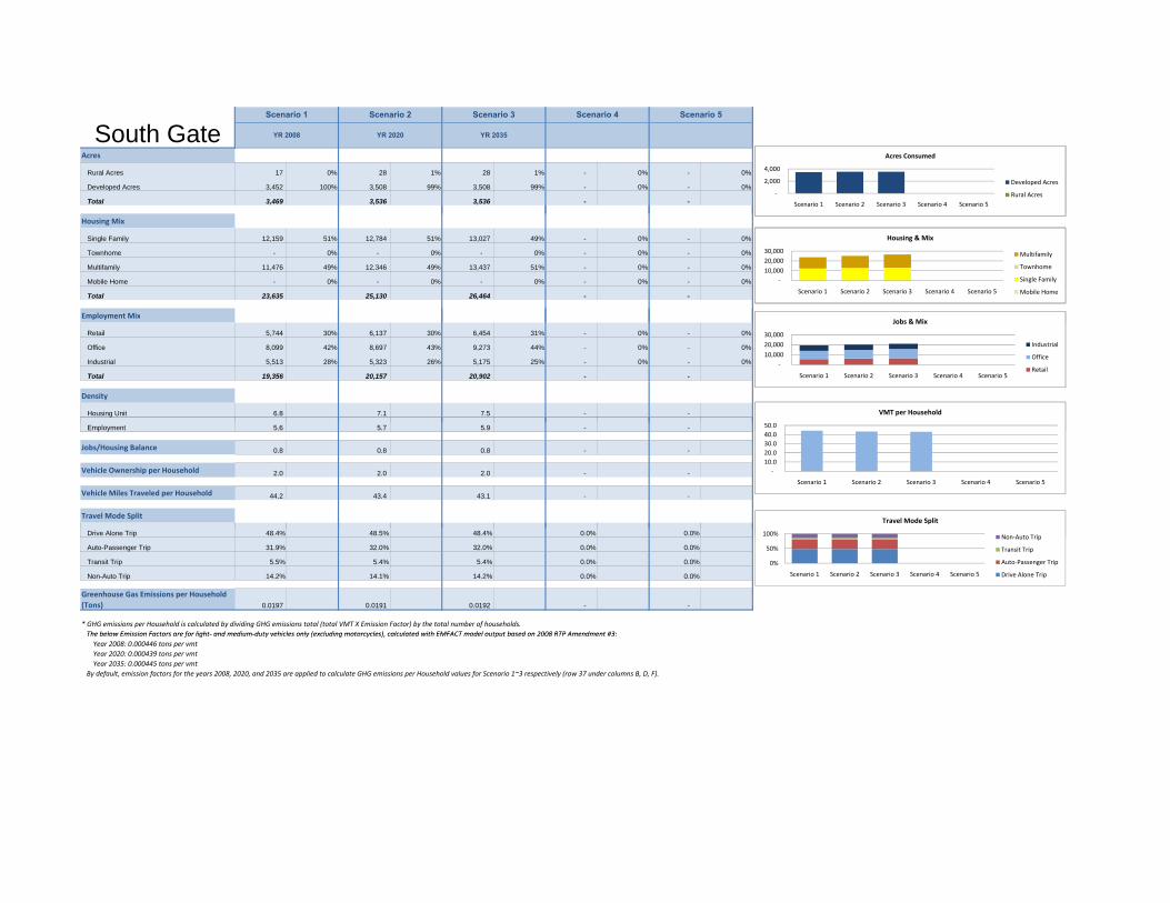
Acres
Rural Acres 17 0% 28 1% 28 1% - 0% - 0%
Developed Acres 3,452 100% 3,508 99% 3,508 99% - 0% - 0%
Total 3,469 3,536 3,536 - -
South GateScenario 5Scenario 1 Scenario 2 Scenario 3 Scenario 4
YR 2008 YR 2020 YR 2035
‐
2,000
4,000
Scenario 1 Scenario 2 Scenario 3 Scenario 4 Scenario 5
Acres Consumed
Developed Acres
Rural Acres
Housing Mix
Single Family 12,159 51% 12,784 51% 13,027 49% - 0% - 0%
Townhome - 0% - 0% - 0% - 0% - 0%
Multifamily 11,476 49% 12,346 49% 13,437 51% - 0% - 0%
Mobile Home - 0% - 0% - 0% - 0% - 0%
Total 23,635 25,130 26,464 - -
Employment Mix
‐
2,000
4,000
Scenario 1 Scenario 2 Scenario 3 Scenario 4 Scenario 5
Acres Consumed
Developed Acres
Rural Acres
‐
10,000
20,000
30,000
Scenario 1 Scenario 2 Scenario 3 Scenario 4 Scenario 5
Housing & Mix
Multifamily
Townhome
Single Family
Mobile Home
Jobs & MixEmployment Mix
Retail 5,744 30% 6,137 30% 6,454 31% - 0% - 0%
Office 8,099 42% 8,697 43% 9,273 44% - 0% - 0%
Industrial 5,513 28% 5,323 26% 5,175 25% - 0% - 0%
Total 19,356 20,157 20,902 - -
Density
Housing Unit 6.8 7.1 7.5 - -
‐
2,000
4,000
Scenario 1 Scenario 2 Scenario 3 Scenario 4 Scenario 5
Acres Consumed
Developed Acres
Rural Acres
‐
10,000
20,000
30,000
Scenario 1 Scenario 2 Scenario 3 Scenario 4 Scenario 5
Housing & Mix
Multifamily
Townhome
Single Family
Mobile Home
‐
10,000
20,000
30,000
Scenario 1 Scenario 2 Scenario 3 Scenario 4 Scenario 5
Jobs & Mix
Industrial
Office
Retail
50.0
VMT per Household
Employment 5.6 5.7 5.9 - -
Jobs/Housing Balance 0.8 0.8 0.8 - -
Vehicle Ownership per Household 2.0 2.0 2.0 - -
Vehicle Miles Traveled per Household 44.2 43.4 43.1 - -
Travel Mode Split
‐
2,000
4,000
Scenario 1 Scenario 2 Scenario 3 Scenario 4 Scenario 5
Acres Consumed
Developed Acres
Rural Acres
‐
10,000
20,000
30,000
Scenario 1 Scenario 2 Scenario 3 Scenario 4 Scenario 5
Housing & Mix
Multifamily
Townhome
Single Family
Mobile Home
‐
10,000
20,000
30,000
Scenario 1 Scenario 2 Scenario 3 Scenario 4 Scenario 5
Jobs & Mix
Industrial
Office
Retail
‐
10.0
20.0
30.0
40.0
50.0
Scenario 1 Scenario 2 Scenario 3 Scenario 4 Scenario 5
VMT per Household
100%
Travel Mode Split
Non Auto TripDrive Alone Trip 48.4% 48.5% 48.4% 0.0% 0.0%
Auto-Passenger Trip 31.9% 32.0% 32.0% 0.0% 0.0%
Transit Trip 5.5% 5.4% 5.4% 0.0% 0.0%
Non-Auto Trip 14.2% 14.1% 14.2% 0.0% 0.0%
Greenhouse Gas Emissions per Household
(Tons) 0.0197 0.0191 0.0192 - -
* GHG emissions per Household is calculated by dividing GHG emissions total (total VMT X Emission Factor) by the total number of households.
The below Emission Factors are for light‐ and medium‐duty vehicles only (excluding motorcycles) calculated with EMFACT model output based on 2008 RTP Amendment #3:
‐
2,000
4,000
Scenario 1 Scenario 2 Scenario 3 Scenario 4 Scenario 5
Acres Consumed
Developed Acres
Rural Acres
‐
10,000
20,000
30,000
Scenario 1 Scenario 2 Scenario 3 Scenario 4 Scenario 5
Housing & Mix
Multifamily
Townhome
Single Family
Mobile Home
‐
10,000
20,000
30,000
Scenario 1 Scenario 2 Scenario 3 Scenario 4 Scenario 5
Jobs & Mix
Industrial
Office
Retail
‐
10.0
20.0
30.0
40.0
50.0
Scenario 1 Scenario 2 Scenario 3 Scenario 4 Scenario 5
VMT per Household
0%
50%
100%
Scenario 1 Scenario 2 Scenario 3 Scenario 4 Scenario 5
Travel Mode Split
Non‐Auto Trip
Transit Trip
Auto‐Passenger Trip
Drive Alone Trip
The below Emission Factors are for light‐ and medium‐duty vehicles only (excluding motorcycles), calculated with EMFACT model output based on 2008 RTP Amendment #3:
Year 2008: 0.000446 tons per vmt
Year 2020: 0.000439 tons per vmt
Year 2035: 0.000445 tons per vmt
By default, emission factors for the years 2008, 2020, and 2035 are applied to calculate GHG emissions per Household values for Scenario 1~3 respectively (row 37 under columns B, D, F).

Acres
Rural Acres 42 2% 86 3% 86 3% - 0% - 0%
Developed Acres 2,523 98% 2,593 97% 2,593 97% - 0% - 0%
Total 2,565 2,679 2,679 - -
VernonScenario 5Scenario 1 Scenario 2 Scenario 3 Scenario 4
YR 2008 YR 2020 YR 2035
‐
2,000
4,000
Scenario 1 Scenario 2 Scenario 3 Scenario 4 Scenario 5
Acres Consumed
Developed Acres
Rural Acres
Housing Mix
Single Family 19 76% 19 76% 19 76% - 0% - 0%
Townhome - 0% - 0% - 0% - 0% - 0%
Multifamily 6 24% 6 24% 6 24% - 0% - 0%
Mobile Home - 0% - 0% - 0% - 0% - 0%
Total 25 25 25 - -
Employment Mix
‐
Scenario 1 Scenario 2 Scenario 3 Scenario 4 Scenario 5
Rural Acres
‐
10
20
30
Scenario 1 Scenario 2 Scenario 3 Scenario 4 Scenario 5
Housing & Mix
Multifamily
Townhome
Single Family
Mobile Home
Jobs & MixEmployment Mix
Retail 12,240 27% 13,899 30% 15,264 31% - 0% - 0%
Office 3,634 8% 4,095 9% 4,531 9% - 0% - 0%
Industrial 28,727 64% 28,852 62% 28,928 59% - 0% - 0%
Total 44,601 46,846 48,723 - -
Density
Housing Unit 0.0 0.0 0.0 - -
‐
20,000
40,000
60,000
Scenario 1 Scenario 2 Scenario 3 Scenario 4 Scenario 5
Jobs & Mix
Industrial
Office
Retail
50.0
VMT per Household
Employment 17.4 17.5 18.2 - -
Jobs/Housing Balance 1,784.0 1,873.9 1,948.9 - -
Vehicle Ownership per Household 2.2 2.2 2.2 - -
Vehicle Miles Traveled per Household 44.2 44.6 44.8 - -
Travel Mode Split
‐
10.0
20.0
30.0
40.0
50.0
Scenario 1 Scenario 2 Scenario 3 Scenario 4 Scenario 5
VMT per Household
100%
Travel Mode Split
Non Auto TripDrive Alone Trip 55.0% 55.0% 55.0% 0.0% 0.0%
Auto-Passenger Trip 34.0% 33.9% 33.8% 0.0% 0.0%
Transit Trip 5.3% 5.4% 5.5% 0.0% 0.0%
Non-Auto Trip 5.7% 5.7% 5.8% 0.0% 0.0%
Greenhouse Gas Emissions per Household
(Tons) 0.0197 0.0196 0.0200 - -
* GHG emissions per Household is calculated by dividing GHG emissions total (total VMT X Emission Factor) by the total number of households.
The below Emission Factors are for light‐ and medium‐duty vehicles only (excluding motorcycles) calculated with EMFACT model output based on 2008 RTP Amendment #3:
0%
50%
100%
Scenario 1 Scenario 2 Scenario 3 Scenario 4 Scenario 5
Travel Mode Split
Non‐Auto Trip
Transit Trip
Auto‐Passenger Trip
Drive Alone Trip
The below Emission Factors are for light‐ and medium‐duty vehicles only (excluding motorcycles), calculated with EMFACT model output based on 2008 RTP Amendment #3:
Year 2008: 0.000446 tons per vmt
Year 2020: 0.000439 tons per vmt
Year 2035: 0.000445 tons per vmt
By default, emission factors for the years 2008, 2020, and 2035 are applied to calculate GHG emissions per Household values for Scenario 1~3 respectively (row 37 under columns B, D, F).

Acres
Rural Acres 165 3% 165 3% 165 3% 24 1% - 0%
Developed Acres 5,386 97% 5,452 97% 5,452 97% 3,460 99% - 0%
Total 5,551 5,617 5,617 3,484 -
blankWhittierScenario 5Scenario 1 Scenario 2 Scenario 3 Scenario 4
YR 2008 YR 2020 YR 2035 blank
‐
5,000
10,000
Scenario 1 Scenario 2 Scenario 3 Scenario 4 Scenario 5
Acres Consumed
Developed Acres
Rural Acres
Housing Mix
Single Family 20,508 73% 21,525 75% 20,851 71% 11,939 81% - 0%
Townhome 296 1% - 0% 315 1% - 0% - 0%
Multifamily 7,479 26% 7,028 25% 8,204 28% 2,781 19% - 0%
Mobile Home - 0% - 0% - 0% - 0% - 0%
Total 28,282 28,554 29,371 14,720 -
Employment Mix
‐
5,000
10,000
Scenario 1 Scenario 2 Scenario 3 Scenario 4 Scenario 5
Acres Consumed
Developed Acres
Rural Acres
‐
20,000
40,000
Scenario 1 Scenario 2 Scenario 3 Scenario 4 Scenario 5
Housing & MixMultifamily
Townhome
Single Family
Mobile Home
Jobs & MixEmployment Mix
Retail 5,750 19% 6,153 20% 6,256 20% 4,588 24% - 0%
Office 21,939 72% 22,113 72% 23,049 73% 8,690 45% - 0%
Industrial 2,603 9% 2,492 8% 2,288 7% 6,070 31% - 0%
Total 30,292 30,758 31,592 19,348 -
Density
Housing Unit 5.1 5.1 5.2 4.2 -
‐
5,000
10,000
Scenario 1 Scenario 2 Scenario 3 Scenario 4 Scenario 5
Acres Consumed
Developed Acres
Rural Acres
‐
20,000
40,000
Scenario 1 Scenario 2 Scenario 3 Scenario 4 Scenario 5
Housing & MixMultifamily
Townhome
Single Family
Mobile Home
‐
20,000
40,000
Scenario 1 Scenario 2 Scenario 3 Scenario 4 Scenario 5
Jobs & Mix
Industrial
Office
Retail
60.0
VMT per Household
Employment 5.5 5.5 5.6 5.6 -
Jobs/Housing Balance 1.1 1.1 1.1 1.3 -
Vehicle Ownership per Household 2.1 2.1 2.0 2.2 -
Vehicle Miles Traveled per Household 49.0 49.0 48.2 50.5 -
Travel Mode Split
‐
5,000
10,000
Scenario 1 Scenario 2 Scenario 3 Scenario 4 Scenario 5
Acres Consumed
Developed Acres
Rural Acres
‐
20,000
40,000
Scenario 1 Scenario 2 Scenario 3 Scenario 4 Scenario 5
Housing & MixMultifamily
Townhome
Single Family
Mobile Home
‐
20,000
40,000
Scenario 1 Scenario 2 Scenario 3 Scenario 4 Scenario 5
Jobs & Mix
Industrial
Office
Retail
‐
20.0
40.0
60.0
Scenario 1 Scenario 2 Scenario 3 Scenario 4 Scenario 5
VMT per Household
100%
Travel Mode SplitNon‐Auto Trip
Transit TripDrive Alone Trip 61.7% 61.8% 61.5% 61.5% 0.0%
Auto-Passenger Trip 27.4% 27.4% 27.3% 27.7% 0.0%
Transit Trip 3.5% 3.4% 3.5% 3.1% 0.0%
Non-Auto Trip 7.4% 7.4% 7.7% 7.6% 0.0%
Greenhouse Gas Emissions per Household
(Tons) 0.0219 0.0215 0.0215 0.0225 -
* GHG emissions per Household is calculated by dividing GHG emissions total (total VMT X Emission Factor) by the total number of households.
The below Emission Factors are for light‐ and medium‐duty vehicles only (excluding motorcycles) calculated with EMFACT model output based on 2008 RTP Amendment #3:
‐
5,000
10,000
Scenario 1 Scenario 2 Scenario 3 Scenario 4 Scenario 5
Acres Consumed
Developed Acres
Rural Acres
‐
20,000
40,000
Scenario 1 Scenario 2 Scenario 3 Scenario 4 Scenario 5
Housing & MixMultifamily
Townhome
Single Family
Mobile Home
‐
20,000
40,000
Scenario 1 Scenario 2 Scenario 3 Scenario 4 Scenario 5
Jobs & Mix
Industrial
Office
Retail
‐
20.0
40.0
60.0
Scenario 1 Scenario 2 Scenario 3 Scenario 4 Scenario 5
VMT per Household
0%
50%
100%
Scenario 1 Scenario 2 Scenario 3 Scenario 4 Scenario 5
Travel Mode SplitNon‐Auto Trip
Transit Trip
Auto‐Passenger Trip
Drive Alone Trip
The below Emission Factors are for light‐ and medium‐duty vehicles only (excluding motorcycles), calculated with EMFACT model output based on 2008 RTP Amendment #3:
Year 2008: 0.000446 tons per vmt
Year 2020: 0.000439 tons per vmt
Year 2035: 0.000445 tons per vmt
By default, emission factors for the years 2008, 2020, and 2035 are applied to calculate GHG emissions per Household values for Scenario 1~3 respectively (row 37 under columns B, D, F).
Appendix G. List of Regional Transportation Strategies in the Gateway Cities, including Analysis

555 12th St reet , Sui te 1600 Oakland, CA 94607
te l 510-873-8700 www.camsys.com fax 510-873-8701
Memorandum
TO: Gateway Cities COG
FROM: Cambridge Systematics, Inc.
DATE: April 25, 2011
RE: Gateway Cities GHG Emission Reduction Benefits from Regional Projects
This memorandum documents the regional greenhouse gas (GHG) emission reduction estimates provided for Gateway Cities Sustainable Communities Strategy (SCS). Those reductions were:
Daily CO2 reduction due to changes in network speed = 7 percent;
Daily CO2 reduction due to reduced VMT (i.e., mode shift) = 1.1 percent; and
Packaging is multiplicative: so the combined benefit is 7.07 percent.
GHG emission reduction estimates from regional actions are based on the expected carbon dioxide (CO2) reductions from the Los Angeles County Metropolitan Transportation Authority (LAMTA) 2009 to 2040 Long-Range Transportation Plan (LRPT)1. The 2009 LRTP project lists confirmed that the Gateway Cities 17 key projects (see Table 1) had been included in LRTP modeling. The 2040 no-build and 2040 plan model summaries for Los Angeles County were obtained from LAMTA. (Gateway Cities specific results were not available.) The datasets are provided as Attachment 1 and Attachment 2, respectively. Calculations were done to reflect the vehicle miles traveled (VMT) reduction and changes in speed distributions.
VMT Reductions
VMT reductions result in a proportional reduction in CO2 emissions. The 2009 LRTP resulted in a 1.1 percent (i.e., 0.011) reduction in VMT for 2040. This 1.1 percent reduction is used for the 2035 horizon year of the SCS.
1 2009 Long-Range Transportation Plan, Technical Document (2009) Los Angeles County Metropolitan Transportation Authority, available online at: http://www.metro.net/projects_studies/images/final-2009-LRTP.pdf, last accessed April 25, 2011.

- 2 -
Table 1. List of Key Regional Projects
Regional Project List Anticipated Completion
2020
I-5 (between I-605 to county line) 2020
I-110 Harbor Transitway HOV lane conversion to HOT lanes 2012
I-710 Arterial Hwy Improvements 2020
I-710 TSM/TDM 2020
2035
BNSF Grade Separation 2035
California High-Speed Rail 2035
Goldline Eastside Extension 2035
Green Line Extension to LAX 2035
I-5 (between I-605 to I-710) 2035
I-5 Arterial Highway Improvements 2035
I-605 Hot Spots 2035
I-710 Freight Corridor 2025
ITS Integration Plan 2025
OLDA Project 2035
Regional Connector 2025
Signal Synchronization of Major Arterials (Re: I-710) 2025
SR 91/I-605/I-405 Arterial Highway Improvements 2035
Speed Distributions Changes
The 2009 LRTP projects alter the average network speeds by targeting bottlenecks. The resulting change in speeds yields a net reduction in CO2 emissions. This emissions benefit was estimated based on the ratio of the Unified cycle correction factor (Equation 1)2, applied by EMFAC2007 to account for the variation in emissions as a function of average trip speed.
2 On-Road Emission Model Methodology Documentation Section 6.2, available on-line at
http://www.arb.ca.gov/msei/onroad/doctable_test.htm, last accessed on April 25, 2011.

- 3 -
. S . . S . Equation 1
Where:
CCF = CO2 Cycle Correction Factor for light- and medium-duty fuel injected vehicles given speed “S”.
For example, the CCF at 18.1 mph is 1.364 and the CCF at 20.9 mph is 1.225; and the emission reduction is therefore 1-1.23/1.36 or 10.1 percent. The calculation for each period modeled for the 2009 LRTP is shown in Table 2 below.
Table2. Unified Cycle Correction Factors Calculations for No-Build and Plan Network Speeds
Period 2040 Plan
VMT 2040 No-Build Average Speed
2040 Plan Average Speed CO2 Reduction
VMT Weighted CO2 reduction
AM Peak 49,433,206 18.1 20.9 10.1% 2.2%
Mid Day 65,659,326 33.3 35.2 3.0% 0.9%
PM Peak 76,791,120 16.1 19 11.2% 3.8%
Night time 35,186,868 46.4 45.2 0.1% 0.0%
Total 227,070,520 7%
Packaging
The emission reduction based on reduced VMT and the emission reduction based on network speed changes are not additive. The factors can be combined as multiplicative adjustments rather than additive adjustments. The combined benefit is therefore 7.07 percent.

- 4 -
Attachment 1. 2040 Plan Model Summery from 2009 LRTP
---------------------------------------------- Daily Los Angeles County Highway Person Trips ---------------------------------------------- HBW Drive Alone 5,399,611 HBW 2 Person Carpool 844,321 HBW 3 Person Carpool 454,525 HBO Drive Alone 5,729,347 HBO 2 Person Carpool 5,397,498 HBO 3 Person Carpool 7,027,722 NHB Drive Alone 6,843,996 NHB 2 Person Carpool 2,868,070 NHB 3 Person Carpool 2,460,488 ---------------------------------------------- ---------------------------------------------- Daily Los Angeles County Highway Vehicle Trips ---------------------------------------------- HBW 5,959,493 HBO 10,557,496 NHB 9,023,559 ---------------------------------------------- ---------------------------------------------- Daily Los Angeles County Transit Person Trips ---------------------------------------------- HBW 851,296 HBO 505,698 NHB 149,232 ---------------------------------------------- -------------------------------------------------------------------------------------- Los Angeles AM 3 Hour Free-Flow VHT Congested VHT VMT SPEED DELAY -------------------------------------------------------------------------------------- Freeway(1,9) 246,232 794,078 17,680,811 22.3 547,845 HOV(5,8) 56,467 157,337 4,059,612 25.8 100,870 Arterials(2,3,4) 674,870 1,216,892 22,578,946 18.6 542,022 Total(1-5,7-9) 1,001,005 2,196,123 45,248,548 20.6 1,195,118 -------------------------------------------------------------------------------------- -------------------------------------------------------------------------------------- Los Angeles AM 1 Hour Free-Flow VHT Congested VHT VMT SPEED DELAY -------------------------------------------------------------------------------------- Freeway(1,9) 98,901 560,411 7,102,449 12.7 461,510 HOV(5,8) 22,568 110,812 1,622,459 14.6 88,244 Arterials(2,3,4) 307,116 857,868 10,217,198 11.9 550,752 Total(1-5,7-9) 439,432 1,545,531 19,372,152 12.5 1,106,099 -------------------------------------------------------------------------------------- -------------------------------------------------------------------------------------- Los Angeles Daily Free-Flow VHT Congested VHT VMT SPEED DELAY -------------------------------------------------------------------------------------- AM 1,169,292 2,364,409 49,433,206 20.9 1,195,118 MD 1,466,445 1,865,362 65,659,326 35.2 398,917 PM 1,855,418 4,035,464 76,791,120 19.0 2,180,047 NT 724,945 779,122 35,186,868 45.2 54,177 Total 5,216,099 9,044,358 227,070,520 25.1 3,828,258 --------------------------------------------------------------------------------------

- 5 -
Attachment 2. 2040 No-Build Model Summary from 2009 LRTP
---------------------------------------------- Daily Los Angeles County Highway Person Trips ---------------------------------------------- HBW Drive Alone 5,440,219 HBW 2 Person Carpool 844,219 HBW 3 Person Carpool 458,703 HBO Drive Alone 5,733,554 HBO 2 Person Carpool 5,402,991 HBO 3 Person Carpool 7,044,461 NHB Drive Alone 6,855,621 NHB 2 Person Carpool 2,870,124 NHB 3 Person Carpool 2,460,100 ---------------------------------------------- ---------------------------------------------- Daily Los Angeles County Highway Vehicle Trips ---------------------------------------------- HBW 6,001,315 HBO 10,569,521 NHB 9,036,093 ---------------------------------------------- ---------------------------------------------- Daily Los Angeles County Transit Person Trips ---------------------------------------------- HBW 781,466 HBO 465,556 NHB 130,569 ---------------------------------------------- -------------------------------------------------------------------------------------- Los Angeles AM 3 Hour Free-Flow VHT Congested VHT VMT SPEED DELAY -------------------------------------------------------------------------------------- Freeway(1,9) 250,374 974,193 17,978,524 18.5 723,819 HOV(5,8) 41,057 111,516 2,951,382 26.5 70,459 Arterials(2,3,4) 725,109 1,494,804 24,129,851 16.1 769,696 Total(1-5,7-9) 1,041,414 2,611,819 46,046,055 17.6 1,570,405 -------------------------------------------------------------------------------------- -------------------------------------------------------------------------------------- Los Angeles AM 1 Hour Free-Flow VHT Congested VHT VMT SPEED DELAY -------------------------------------------------------------------------------------- Freeway(1,9) 100,554 683,446 7,221,179 10.6 582,892 HOV(5,8) 16,304 77,542 1,172,001 15.1 61,238 Arterials(2,3,4) 327,764 1,103,914 10,864,077 9.8 776,151 Total(1-5,7-9) 456,380 1,886,573 19,723,507 10.5 1,430,193 -------------------------------------------------------------------------------------- -------------------------------------------------------------------------------------- Los Angeles Daily Free-Flow VHT Congested VHT VMT SPEED DELAY -------------------------------------------------------------------------------------- AM 1,211,452 2,781,857 50,267,789 18.1 1,570,405 MD 1,500,572 1,980,730 65,927,142 33.3 480,158 PM 1,922,297 4,842,504 78,201,854 16.1 2,920,207 NT 730,867 768,483 35,681,328 46.4 37,616 Total 5,365,189 10,373,575 230,078,112 22.2 5,008,386 --------------------------------------------------------------------------------------

Appendix H. Analysis of Interactive Effects Contributing to Further GHG Reduction in the Gateway Cities
Gateway Cities Council of Governments Subregional Sustainable Communities Strategy Appendix
Cambridge Systematics, Inc. H-1
H. Land Use – Regional Transit Capacity Expansion Interaction
Overview
The interaction between new development and redevelopment in Gateway Cities as modeled through the Sustainability Tool (ST) and regional public transportation projects funded under Measure R is a critical component of estimating GHG emission reductions in 2020 and 2035. This interaction is assumed to represent all components of the 4D concept – that households in communities featuring high density development, a diverse and balanced mix of uses, a high quality pedestrian environment, and superior access to regional opportunities via transit are much less auto dependent.
The element of the 4Ds under more careful consideration in the Gateway Cities SCS analysis is with regard to change in transit access and level of service. The reason for this additional attention is the recognition of the significant role that regional transit projects in the RTP and funded under Measure R will play in future development patterns and travel choices in the Gateway Cities.
Assessment Process in Gateway Cities SCS
There are two primary components to the land use-regional transit capacity expansion interaction under consideration in the SCS:
1. Regional Transit Walk Access – There are two potential interactions to consider:
a. Residential and commercial development and redevelopment identified in the Gateway Cities adjacent to existing transit stations will on average generate less VMT per household than households not adjacent to transit. This interaction is accounted for in the ST.
b. The improvement of transit access to regional destinations outside the Gateway Cities and new high capacity and frequent regional transit service in Gateway Cities as identified in the RTP and Measure R project list improves the level of service and utility of the transit mode leading to mode shift from vehicle-based trips.
2. Transit-Oriented Development (TOD) Opportunity – New or improved transit stations attract new TOD, consisting of high-density, mixed residential and commercial development with a higher propensity for transit trips.
Regional Transit Walk Access
The Sustainability Tool has functionality that estimates the interactions between land use (expressed as the 4Ds: density, diversity, design, destination) and

Gateway Cities Council of Governments Subregional Sustainable Communities Strategy Appendix
H-2 Cambridge Systematics, Inc.
proximity to a fixed-guideway transit node (defined as within ½ mile). The ST subdivides the growth forecasts from the cities into 5.5-acre grid cells, overlays the data with existing transit facilities, and flags all cells within a one-half mile of transit station locations and one-quarter mile of bus transit routes.
In the ST, regional transit walk access is an environmental (nondemographic based) predictor of household transit trips, with an average reported elasticity of 0.25 (meaning that for every 10-percent increase in households flagged with regional transit walk access, there is a 2.5-percent increase in transit trips).
The GHG reduction estimates developed through the ST reflects the benefit of growth and land use change within the Gateway Cities through 2035 overlaid on the existing regional transit network.
The ST does not consider the additional VMT reduction that could occur in the Gateway Cities as a result of long-range implementation of Measure R transit projects. Projects in the Measure R plan anticipated to be completed by 2035 that will affect travel in Gateway Cities includes:
1. The Gold Line Eastside Extension,
2. The Orange Line Development Authority (OLDA) grade-separated regional transit project,
3. The Regional Connector project linking the Blue Line to other MTA facilities in Downtown Los Angeles, and
4. The Green Line extension to LAX.
These projects will positively affect transit ridership in the Gateway Cities in two ways: 1) the projects will improve regional access to attractions, employment, and services for Gateway Cities households; and 2) the projects will provide a new fixed guideway transit alternative to private vehicle or bus transit trips.
Inside Gateway Cities, the primary project of interest is the OLDA project. It is likely that most, if not all, of the households adjacent to this project already have access to transit. The ST currently applies the same regional transit walk access approach for the households in these grid cells, however, uses a one-quarter-mile access buffer.
Fixed guideway transit tends to be more attractive than bus transit to discretionary travelers (people who have the option of driving), including commuters, visitors, and people traveling to major sporting and cultural events if they are located along transit lines. To reflect the transition from bus to fixed-guideway transit access, an assumption that the regional transit walk access elasticity increases from 0.17 for bus to 0.33 for rail is reasonable for these discretionary trips. Essentially, travelers with existing access to bus transit, which will in the future have access to rail transit, will be 1.5 to 2 times as likely to choose transit than before (while controlling for socioeconomic variables). Results from travel demand modeling activities completed for these regional transit projects will effectively demonstrate the benefit of this interaction as well.
Gateway Cities Council of Governments Subregional Sustainable Communities Strategy Appendix
Cambridge Systematics, Inc. H-3
TOD Opportunity
In expanding transit corridors in California and elsewhere, the presence of new, high capacity, high level of service public transportation options has been shown to be a catalyst for new or redevelopment. Through zoning codes and development regulations, cities may support development of these areas through reduced parking requirements, tax increment financing, and other incentives to maximize the opportunity for development and capitalize on their investment in transit.
It is uncertain how much the opportunity for rezoning and eventual redevelopment of land uses near planned transit stations is incorporated into city general plans. The only project in the Measure R plan anticipated to be completed by 2035 that could facilitate TOD in Gateway Cities is the Orange Line Development Authority grade-separated high-speed regional transit project planned to provide access to Vernon, Maywood, Bell, Huntington Park, Cudahy, Downey, South Gate, Paramount, Artesia, Bellflower, and Cerritos.
In addition, other regional transit projects which increase the level of service and accessibility to attractions outside the Gateway Cities (for example such as new Green Line access to LAX) could also, to a lesser degree than above, facilitate TOD at existing transit stations in the Gateway Cities. It is likely, that the benefits from TOD at these locations would occur sooner than TOD associated with the OLDA project given that the transit infrastructure is already in place.
The level to which growth in the Gateway Cities could intensify or be redistributed to focus in areas adjacent to new fixed-guideway transit stations is dependent on available development capacity, supporting infrastructure, zoning and development regulations, and future economic and market conditions. The example analysis of this interaction considers the affect of TOD in areas within one-eighth mile of Orange Line transit stations.
Results
The data summarized in Table H.1 reflects the range of potential benefits resulting from the interaction between land use and Measure R transit projects in the Gateway Cities in 2035. Given the anticipated long timeframe for implementation of the Measure R transit projects, as well as the long lead time for redevelopment activities adjacent to new transit, the resulting GHG reductions associated with this interaction is only considered for 2035.

Gateway Cities Council of Governments Subregional Sustainable Communities Strategy Appendix
H-4 Cambridge Systematics, Inc.
Table H.1 Gateway Cities SCS – GHG Reduction from Land Use and Regional Transit Interactions
Gateway Cities – Land Use and Regional Transit Interaction 2035
Interaction 1 – Regional Walk Access
Improved Access to Regional Destinations
Average Daily VMT per Household in Gateway Cities 42.5
Total Daily GHG Reduction (lbs GHG per capita) 0.041-0.062
New Access to Fixed Guideway Transit
Total Households within 1/2 mile of “Orange Line” Station Locations 1 40,075
Total Daily GHG Reduction (lbs GHG per capita) 0.021-0.042
Interaction 2 – TOD
Target Density Range in TOD Station Areas (TOD defined as 1/8 mile of station)2 23.7-60.7 hu/acre
Total Households in TOD Station Areas 8,186-20,966
Total Daily GHG Reduction (lbs GHG per capita) 0.058-0.073
Total Daily GHG Reduction (lbs GHG per capita) 0.120-0.177
Notes:
1. Assumes constant household density within each city based on 2035 forecasts.
2. Apply characteristics of range “Town Residential High Mix to Town Residential Low Mix” to TOD station areas.
Appendix I. CEQA Streamlining
Gateway Cities Council of Governments Subregional Sustainable Communities Strategy Appendix
Cambridge Systematics, Inc. I-1
I. CEQA Streamlining: Existing Land Use, Density, and Building Intensity Data
SB 375 provides incentives in the form of CEQA streamlining to support community designs that help reduce GHG emissions. To take advantage of these CEQA streamlining provisions in SB 375, projects must prequalify based on two criteria:
1. A project must be consistent with the land use designation, density, building intensity, and applicable policies in an approved SCS or Alternative Planning Strategy1
2. A project must be considered a Transit Priority Project (TPP) or a Residential/Mixed Use Residential Project (as defined in SB 375).
; and
To help Gateway Cities Council of Governments (GCCOG) jurisdictions take advantage of the CEQA streamlining provisions in SB 375, SCAG will include maps in the regional 2012 RTP/SCS in order to show the uses, densities, intensities, and locations for future development; and in order to facilitate subsequent project consistency findings. These maps will use the GCCOG dataset as reviewed and approved by GCCOG. SCAG, in consultation with GCCOG and their jurisdictions, may provide more detail to allow interested jurisdictions to take advantage of the CEQA streamlining provisions in SB 375. SCAG will only show more land use detail, where a jurisdiction has acknowledged that the land use information is based on their input and approved of its being displayed in the adopted plan.
To facilitate SB 375 CEQA Streamlining, individual GCCOG jurisdictions are asked to provide detailed land use information (uses, densities, intensities at a defined geographic level) to SCAG. These data are called out in the SCAG Framework and Guidelines and the legislation specific to the streamlining
1 CARB will review the regional SCS to accept or reject SCAG’s determination
whether or not the implementation of the SCS would achieve the GHG emission reduction targets for the region. If the regional targets cannot be achieved by the regional SCS, then SCAG must prepare an Alternative Planning Strategy (APS). An APS is a separate document from the RTP and describes how the targets could be achieved through alternative development patterns, infrastructure, or additional transportation measures or policies.

Gateway Cities Council of Governments Subregional Sustainable Communities Strategy Appendix
I-2 Cambridge Systematics, Inc.
provisions. Additionally, or in lieu of detailed land use information, jurisdictions may work with SCAG in designating the appropriate regional “development type” in locations for potential future projects. Jurisdictions themselves will determine whether a particular project meets the CEQA streamlining qualifications, including making the consistency finding. If a jurisdiction does not participate in the SCS data collection effort for existing land use, density, and building intensity, there is no direct adverse consequence due to not providing input.
In order to provide the most accurate data possible for the GCCOG subregion, and to preserve individual jurisdictions’ general plan and existing data accuracy, detail, and integrity, and to meet the requirements under SB 375 for purposes of CEQA streamlining, SCAG prepared and provided GCCOG local jurisdictions with a set of data/GIS maps of detailed land use information, including General Plan, zoning, and existing general land use designation, density and building intensity data and maps, all for the jurisdictions’ review and comment. The data was provided in the format of the Sustainability Tool by January 31, 2011. GCCOG consultants helped to extract the data for review during the February 16 workshop at the GCCOG offices in Paramount, California.
The information contained in the data packets document was developed and/or collected by the staff in the Data and GIS group in the Department of Research, Analysis, and Information Services (RAIS) under the Land Use and Environmental Planning (LUEP) Division at SCAG. The SCAG Data/Map Guide included information on the sources, methodologies, and contents of each dataset. These data/GIS maps are identified in SB 375 as required to be considered in the SCS development to address the requirements of SB 375 and its implementation for purposes of CEQA streamlining. Comments and corrections from subregions and local jurisdictions are due to SCAG as part of the Gateway SCS process by April 29, 2011. The list of data/GIS maps included in the SCAG map and data packets, along with the review requested of GCCOG jurisdictions, appears as Table I.1 below.

Gateway Cities Council of Governments Subregional Sustainable Communities Strategy Appendix
Cambridge Systematics, Inc. I-3
Table I.1 Contents of the SCAG Map and Data from the Sustainability Tool Category GIS Shapefile Available?
Land Use
General Plan Yes
Zoning Yes
Existing Land Use of 2008 Yes
Geographical Boundaries
Jurisdictional Boundary and Sphere of Influence Yes
Census Tract Boundary Yes
TAZ Boundary Yes
Transit Priority Projects
Major Stops & High Quality Transit Corridors Yes
Resource Areas & Farmland
Endangered Species and Plants Yes
Flood Areas Yes
Natural Areas Yes
Open Space and Parks Yes
Farmland Yes
Background: Existing Land Use, Density, and Building Intensity In 2008 and early 2009, SCAG began to collect the general plan and zoning information from local jurisdictions, with year adopted ranging from 1971 to 2009 by jurisdiction. The general plan and zoning documents, maps, and/or GIS shapefiles collected were coded into GIS shapefiles at parcel level. Parcel data were acquired from Digital Map Product for Gateway Cities COG. Beginning in July 2009, SCAG communicated with local jurisdictions, and revised the general plan and zoning data based on the results of the local review. Through a process of collecting general plan and zoning documents and receiving comments from local jurisdictions, information included in the data packets reflected the local inputs received by January 31, 2010. SCAG continues to receive local input, and will incorporate them into the database. General Plan data are shown at a parcel level; in many areas, they depict a local agency’s adopted documents accurately. However, the data shown in some areas may be generalized or inaccurate for many reasons, a primary reason because the parcel-level database representing general plan does not support multiple uses or designations on a single parcel (either splitting the parcel or representing overlays). Additionally, data on building size, existing use, and other specific parcel-related information that SCAG collected from other original data sources, such as the Gateway Cities

Gateway Cities Council of Governments Subregional Sustainable Communities Strategy Appendix
I-4 Cambridge Systematics, Inc.
County Assessor’s Office, may have been in error and/or not up to date. Due to these inaccuracies and limitations, if site-specific data is necessary, users should always reference a local agency’s adopted documents or field surveys to determine actual land use designations.
At the jurisdiction level, both general plan land use and zoning maps are prepared with the land use or zoning codes used in each local jurisdiction. General Plan land use maps are also available at larger geographic levels, such as subregion, county, or the entire SCAG region with SCAG’s standardized General Plan codes. For detailed information on the standardized codes, please refer to SCAG’s General Plan Code Table.
SCAG prepared three sets of land use maps (General Plan Land Use, Zoning and 2008 Existing Land Use) at parcel level. The three land use maps were originally provided to local jurisdictions in September/October 2009. Based on one-on-one meetings and communication with local jurisdictions throughout the first round outreach (July 2009 to January 2010) the Data/Map packets of existing land use, density, and building intensity data transmitted to Gateway Cities COG jurisdictions in February 2011 reflect the local inputs received by January 31, 2010.
Gateway Cities Jurisdiction Review Process GCCOG distributed the electronic files and hard copies to Gateway cities for review. They were asked to review and submit updates and comments for purposes of SB 375 CEQA streamlining and with regard to the land use strategies developed for GHG reduction in SB 375. All GCCOG jurisdictions received the SCAG datasets in both electronic and hard copy format. Most, but not all, GCCGOG jurisdictions reviewed the data for purposes of SB 375.
SCAG staff presented a data orientation and review session to the GCCOG on February 16, 2011, at a technical workshop held at the Gateway COG. Additionally, SCAG staff was available and conducted one-on-one meetings with cities who were interested in modifying and/or reviewing their land use during the last week of March 2011 to provide technical data and GIS assistance to GCCOG jurisdictions with limited data/GIS capability that needed assistance in the Data/Map review.
Based upon parcel level data originally provided by SCAG, GCCOG jurisdictions reviewed the data to various degrees for purposes of CEQA streamlining.
Results The results of that process have been provided electronically to SCAG through the Sustainability Tool. For a select number of cities, modifications were made in conjunction with SCAG staff. For the remainder, default scenarios were used, which were part of the SCAG original dataset.
Gateway Cities Council of Governments Subregional Sustainable Communities Strategy Appendix
Cambridge Systematics, Inc. I-5
In Appendix J, individual jurisdiction General Plans are presented along with web address links to individual jurisdictions’ General Plans. Individual jurisdiction General Plans are always considered the final and ultimate authority on land use and zoning, especially for those jurisdictions that opted not to review the SCAG data.
For those jurisdictions that did not fully review, there are some limitations, conditions, and caveats to the existing land use, density, and building intensity data. Data provided by SCAG on land use is in some areas inaccurate and/or generalized. Because the parcel-level database representing existing land use, general plan, and zoning data does not support multiple uses or designations on a single parcel (either splitting the parcel or representing overlays, such as zoning overlays), the data ultimately shown may generalize the data and thus not accurately depict a local government’s adopted general plan or zoning or the existing land use on the site (including land use designated through a development or other legal agreement).
Due to these caveats and limitation, if site-specific data is necessary, users should always reference and rely on individual Gateway Cities jurisdiction general plans as the final authority. A local agency’s adopted documents are always the final say on allowable land use designations and zoning, and actual site visits or field surveys to determine densities and building intensities should be undertaken.


