Download - Solar convection - Max Planck Society

Solar convectionIn addition to radiation, convection is the main form of energy transport in solar interior and lower atmosphere. Convection dominates just below the solar surface and produces most structures the lower solar atmosphere

The convection zone Through the outermost 30% of solar interior, energy is
transported by convection instead of by radiation
In this layer the gas is convectively unstable.
I.e. the process changes from a random walk of the photons through the radiative zone (due to high density, the mean free path in the core is well below a millimeter) to convective energy transport
The unstable region ends just below the solar surface. I.e. the visible signs of convection are actually due to overshooting (see following slides)
t radiative ~ 105 years >> tconvective ~ weeks
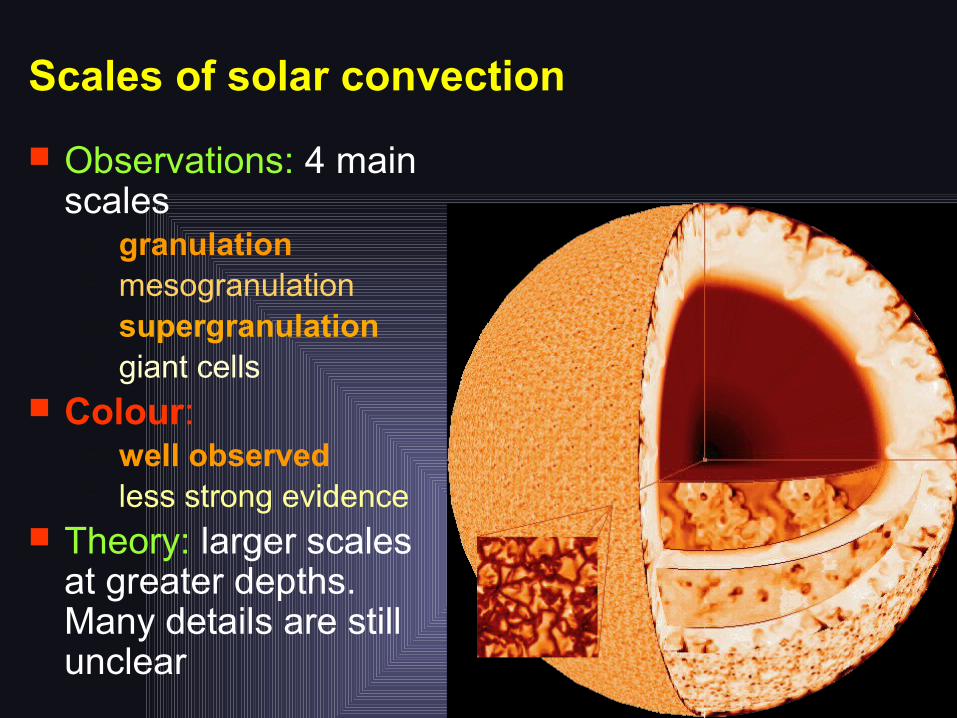
Scales of solar convection
Observations: 4 main scales
– granulation– mesogranulation– supergranulation– giant cells
Colour: – well observed – less strong evidence
Theory: larger scales at greater depths. Many details are still unclear

Surface manifestation of convection: Granulation Typical size: 1-2 Mm Lifetime: 5-8 min Velocities: 1 km/s (but
peak velocities > 10 km/s, i.e. supersonic)
Brightness contrast: ~15% in visible (green) continuum
All quantities show a continuous distribution of values
At any one time 106 granules on Sun
Brightness
LOS Velocity

Surface manifesttion of convection: Supergranulation
1 h average of MDI Dopplergrams (averages out oscillations)
Dark-bright: flows towards/away from observer
No supergranules visible at disk centre velocity is mainly horizontal
Size: 20-30 Mm, lifetime: days, horiz. speed: 400 m/s, no contrast in visible

Supergranules seen by SUMER
Si I 1256 Å full disk scan by SUMER in 1996
Bright network: found at edges of supergranulation cells
Darker cells: supergranules
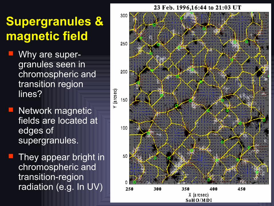
Supergranules & magnetic field Why are super-
granules seen in chromospheric and transition region lines?
Network magnetic fields are located at edges of supergranules.
They appear bright in chromospheric and transition-region radiation (e.g. In UV)

Onset of convection
Schwarzschild’s instability criterion
Consider a rising bubble of gas:
ρ* z-Δz ↑ ρ ρ0 ( = ρ) z
bubble surroundings depth
Condition for convective instability:
If instability condition is fulfilled displaced bubble keeps moving ever faster in same direction
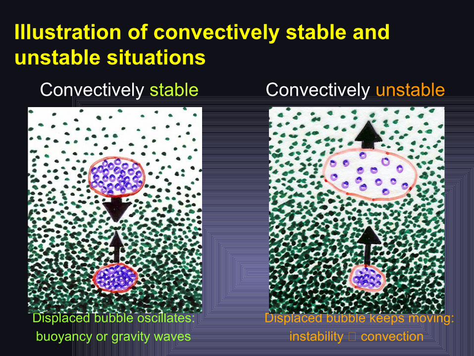
Illustration of convectively stable and unstable situations
Convectively stable Convectively unstable
Displaced bubble oscillates: Displaced bubble keeps moving:
buoyancy or gravity waves instability convection

Onset of convection II
For small Δz, bubble will not have time to exchange heat with surroundings: adiabatic behaviour. Convectively unstable if:
: stellar density gradient in radiative equilibrium
: adiabatic density gradient
Often instead of another gradient is considered: . A larger implies a smaller

Onset of convection III
Rewriting in terms of temperature and pressure:
= adiabatic temperature gradient
gradient for radiative equilibrium
Schwarzschild’s convective instability criterion:
Convectively stable Convectively unstable
-z -zadiabatic
adiabatic
Radiative
Radiativeaaa
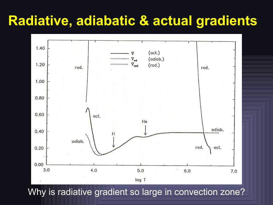
Radiative, adiabatic & actual gradients
Why is radiative gradient so large in convection zone?

Ionisation of H and He Radiative gradient is large where opacity increases rapidly
with depth. This happens where common elements get ionized (i.e. many electrons are released, increasing f-f opacity)
Degree of ionisation depends on T and ne :– H ionisation happens just below solar surface
– He → He+ + e- happens 7000 km below surface
– He+ → He++ + e- happens 30’000 km below surface
Since H is most abundant, it provides most electrons (largest opacity) and drives convection most strongly
At still greater depth, ionization of other elements also provides a minor contribution.

Convective overshoot
Due to their inertia, the packets of gas reaching the boundary of convection zone pass into the convectively stable layers, where they are braked & finally stopped
overshooting convection
Typical width of overshoot layer: order of Hp
This happens at both the bottom and top boundaries of the CZ and is important:
– top boundary: Granulation is overshooting material. Hp ≈ 150 km in photosphere
– bottom boundary: the overshoot layer allows B-field to be stored → seat of the dynamo?
buoyancy
buoyancy
solar surface

Convection Simulations
3-D hydrodynamic simulations reproduce a number of observations and provide new insights into solar convection
These codes solve for mass conservation, momentum conservation (force balance, Navier-Stokes equation), and energy conservation including as many terms as feasible
Problem: Simulations can only cover 2-3 orders of magnitude in length scale (due to limitations in computing power), while the physical processes on the Sun act over at least 6 orders of magnitude
Also, simulations can only cover a part of the size range of solar convection, either granulation, supergranulation, or giant cells, but not all

Simulations of solar granulation
Solution of Navier-Stokes equation etc. describing fluid dynamics in a box (6000 km x 6000 km x 1400 km) containing
the solar surface. Realistic looking granulation is formed.
6 M
m

Testing the simulations
Comparison between observed and computed scenes for spectral lines in yhr Fraunhofer g-band (i.e. lines of an
absorption band of the CH molecule): Molecules are dissociated at relatively low temperatures, so that even slightly hotter than
average features appear rather bright
Simulated Observed

Relation between granules and supergranules Downflows of granules continue to bottom of
simulations, but the intergranular lanes break up into isolated narrow downflow plumes.
I.e. topology of flow reverses with depth: – At surface: isolated upflows, connected downflows
– At depth: connected upflows, isolated downflows
Idea put forward by Spruit et al. 1990: At increasingly greater depth the narrow downflows from different granules merge, forming a larger and less fine-meshed network that outlines the supergranules

Increasing size of convection cells with depth

What message does sunlight carry?
Solar radiation and spectrum

Solar spectrumApproximately 50x better spectrally resolved than previous spectrum
H
Na I D
Mg Ib
g-Band (CH molecular band)

Absorption and emission lines
Continuousspectrum
continuum + absorption lines
Emission lines
Hδ Hγ Hβ Hα

Radiation: definitions Intensity I = energy radiated per wavelength interval,
surface area, unit angle and time interval
Flux F = I in direction of observer integrated over the whole Sun:
where
radiation emitted by Sun (or star) in direction of observer
Irradiance solar flux at 1AU = – Spectral irradiance Sλ = irradiance per unit wavelength– Total irradiance Stot = irradiance integrated over all λ

Hydrostatic equilibrium Sun is (nearly) hydrostatically stratified (this is the case even
in the turbulent convection zone). I.e. gas satisfies:
(P pressure, g gravitational accelaration, ρ density, μ mean molecular weight, R gas constant)
Solution for constant temperature:
pressure drops exponentially with height
Here H is the pressure scale height. H ~ T 1/2 and varies between 100 km in photosphere (solar surface) and ~104 km at base of convection zone and in corona

Optical depth
Let axis point in the direction of light propagation
Optical depth: ,
where is the absorption coefficient [cm-1] and is the frequency of the radiation. Light only knows about the scale and is unaware of
Integration over :
Every has its own scale (note that the scales are floating, no constant of integration is fixed)

The Sun in white light: Limb darkening
In the visible, Sun’s limb is darker than solar disc centre ( limb darkening)
Since intensity ~ Planck function, Bν(T), T is lower near limb
Due to grazing incidence we see higher near limb: T decreases outward

Rays emerging from disk-centre and limb
Path travelled by light emerging at centre of
solar diskPath travelled by light
emerging near solar limb
Rays near solar limb originate higher in atmosphere since they travel 1/cosθ longer path in atmosphere same number of absorbing atoms along path is reached at a greater height
θ

Limb darkening vs. wavelength λ
Short λ: large limb darkening;
Long λ: small limb darkening
Departure from straight line: limb darkening is more complex than
950 nm
350 nm
For most purposes it is sufficient to add a quadratic term

The Sun in the FUV: Limb brightening
nm, Sun’s limb is brighter than disc centre ( limb brightening)
Most FUV spectral lines are optically thin
Optically thin radiation (i.e. throughout atmosphere) comes from the same height at all
Intensity ~ thickness of layer contributing to it. Near limb this layer is thicker
C IV 154 nm
SUMER/SOHO

The Sun in the FUV: Limb brightening
Limb brightening in optically thin lines does NOT imply that temperature increases outwards (although by chance it does in these layers....)
Si I 125.6 nm
SUMER/SOHO

Solar irradiance spectrumIrradiance = solar flux at 1AU Spectrum is similar to, butnot equal toPlanck function Radiation comes from layers with diff. temperatures.
Often usedtemperaturemeasure for stars: Effective temp: σT4eff = Area under flux curve
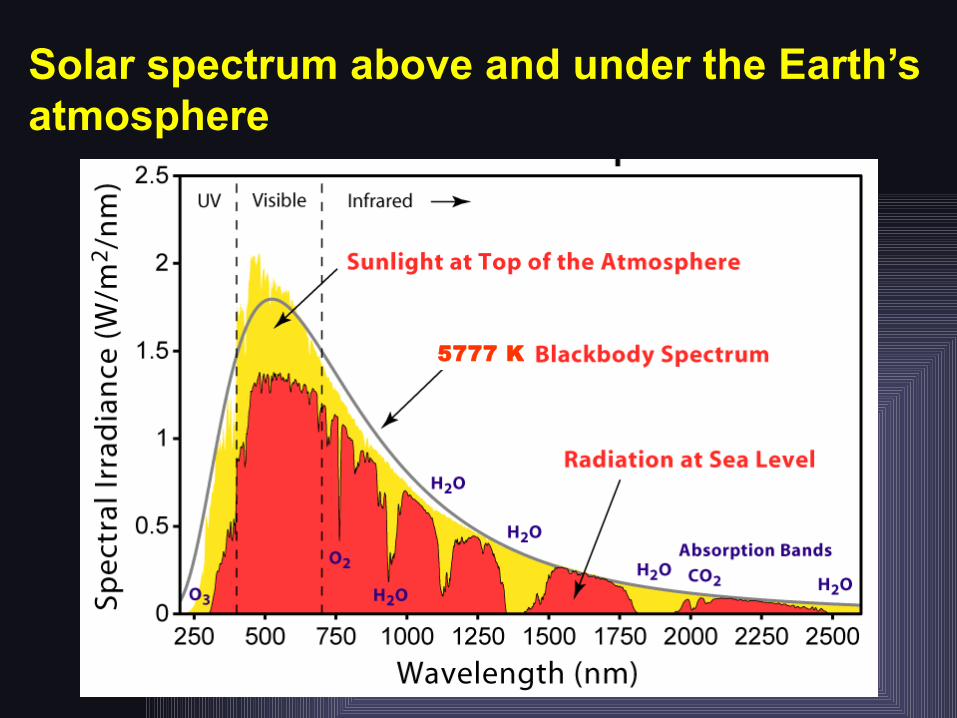
Solar spectrum above and under the Earth’s atmosphere
5777 K

Absorption in the Earth’s atmosphere
Space Observationsneeded
Balloons
Ground

Planck’s function
Amplitude increases rapidly with temperature, area increases ~T 4 (Stefan-Boltzmann law) from λ-integrated intensity we get (effective) temperature
Wavelength of maximum changes linearly with temperature (Wien’s law)
Planck function is more sensitive to T at short λ than at long λ
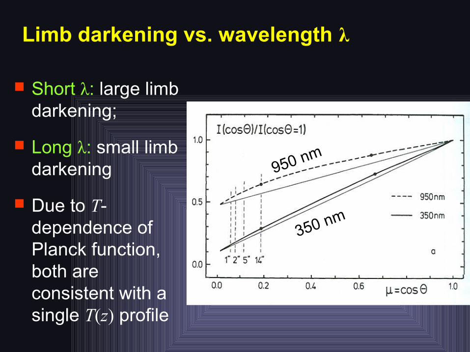
Limb darkening vs. wavelength λ
Short λ: large limb darkening;
Long λ: small limb darkening
Due to T-dependence of Planck function, both are consistent with a single T(z) profile
950 nm
350 nm

Optical depth and solar surface
Radiation at frequency ν escaping from the Sun is emitted mainly at heights around τν ≈ 1.
At wavelengths at which κν is larger, the radiation comes from higher layers in the atmosphere.
In solar atmosphere κν is small in visible and near IR, but large in UV and Far-IR We see deepest in visible and Near-IR, but sample higher layers at shorter and longer wavelengths.

Height of τ = 1, brightness temperature and continuum opacity vs. λ
1.6μm
UVIR

Visible

Solar UV spectrum
Note the transition from absorption lines (for λ > 2000Å) to emission lines (for λ < 2000Å)

FUV spectrum
λ (Å) 800 1000 1200 1400 1600
Ly α
Lyman continuum
The solar spectrum from 670 Å to 1620 Å measured by SUMER on SOHO (logarithmic intensity scale)

Transitions forming lines and continua: free-free continua
Electron scattering,f-f transition:
Continuum emission
Energy: increases radially outwards
Photon (low energy)
Drop in energy of
Upper energy level
Lower energy level

Transitions forming lines and continua: recombination continua
Recombination, b-f
transition: Continuum
emission
Photon, usuallyhigher energy
Energy: increases radially outwards
Upper energy level
Lower energy level
Collisional ionisation
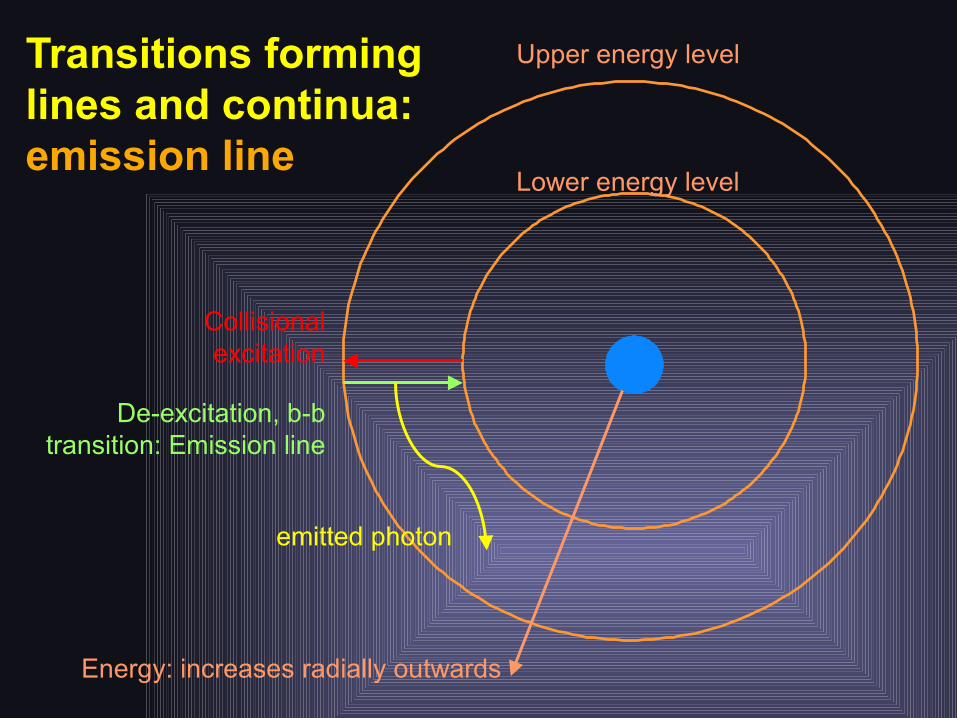
Transitions forming lines and continua: emission line
De-excitation, b-b transition: Emission line
emitted photon
Collisional excitation
Energy: increases radially outwards
Upper energy level
Lower energy level

Transitions forming lines and continua: absorption line
Excitation, b-b transition:
Absorption line
absorbed photon
Energy: increases radially outwards
Upper energy level
Lower energy level
Collisional de-excitation

The solar spectrum: continua with absorption and emission lines
Solar spectrum changes in character at different λ
X-rays: Emission lines of highly ionized species
EUV - FUV: Emission lines of neutral to multiply ionized species plus recombination continua
NUV: stronger recombination (bound-free, or b-f) continua and absorption lines
Visible: H- b-f continuum with absorption lines
FIR: H- f-f (free-free) continuum, increasingly cleaner (i.e. less lines as λ increases, except molecular bands)
Radio: thermal and, at longer λ, increasingly non-thermal continua

Typical scenario in solar atmosphere (not to scale)
Height z
Tem
pera
ture
T,
Sou
rce
func
t.Log(p ress ure
f-f and b-f continuum
of H-
Absorption lines Recombination
continua
Lines w. emission coresEmission lines
Recombin. continua
Emission lines;
Recomb. continua
Visible / NIR visble / FIR / UV EUV/X-ray/Radio

When are emission, when absorption lines formed?
Continua are in general formed the deepest in the atmosphere (or at similar heights as the lines)
Absorption lines are formed when the continuum is strong and the temperature (source function) drops outwards (most effective for high density gas)
– Photons excite the atom into a higher state. For a high gas density, atoms are de-excited by collisions & the absorbed photon is destroyed
Emission lines are formed when the temperature (source function) rises outwards and gas density is low:
– If the gas density is low an excited atom decays spontaneously to a lower state, emitting a photon

Radiative Transfer
If a medium is not optically thin, then radiation interacts with matter and its transfer must be taken into account
Geometry:
Equation of radiative transfer:
where is intensity and is the source function. . Here emissivity , abs. coefficient κν . , where angle of line-of-sight to surface normal
The physics is hidden in and , i.e. in and . They are functions of and elemental abundances
Simple expression for valid in solar photosphere: Planck function
z
To observer

Radiative Transfer in a spectral line
A spectral line has extra absorption: let , κC be absorption coefficient in spectral line & in continuum, respectively
Equation of radiative transfer for the line:
where SL is the line source function, which we assume here to be equal to the Planck function

Milne-Eddington solution
A simple analytical solution for a spectral line exists for a Milne-Eddington atmosphere, i.e. independent of τC and SL depending only linearly on :
I(μ)/IC(μ) = continuum-normalized emergent intensity (residual intensity), where Here is line center absorption coefficient, is line profile shape
The term takes care of line saturation.
As line opacity, ~η0, increases, initially decreases, but for large η0 saturates around

Illustration of line saturation: weak and strong spectral lines 4 spectral lines
computed using Milne-Eddington assumption
Different strengths, i.e. different number of absorbing atoms along LOS. Parameterized by η0
As η0 increases the line initially becomes deeper, then wider, finally showing prominent line wings Figure kindly provide by J.M. Borrero

Diagnostic power of spectral lines
Different parameters describing line strength and line shape contain information on physical parameters of the solar/stellar atmosphere:
– Doppler shift of line: (net) flows in the LOS direction
– Line width: temperature and turbulent velocity
– Area under the line (equivalent width): elemental abundance, temperature (via ionisation and excitation balance)
– Line depth: temperature (and temperature gradient)
– Line asymmetry: velocity gradients, v, T inhomogenieties
– Wings of strong lines: gas pressure
– Polarisation and splitting: magnetic field
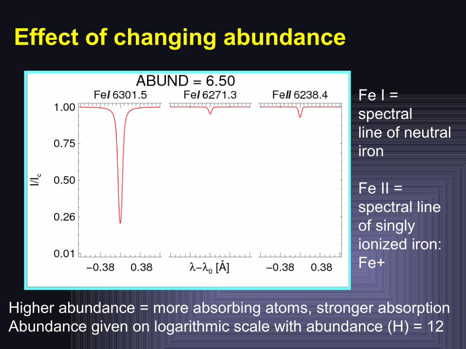
Effect of changing abundance
Higher abundance = more absorbing atoms, stronger absorptionAbundance given on logarithmic scale with abundance (H) = 12
Fe I = spectralline of neutral iron
Fe II = spectral line of singly ionized iron: Fe+

Effect of changing temperature on absorption lines
Low temperatures: Fe is mainly neutral strong Fe I, weak Fe II linesHigh temperatures: Fe gets ionized Fe II strengthens relative to Fe I Very high temperatures: Fe gets doubly ionized Fe II also gets weak

Effect of changing line-of-sight velocity on absorption lines
Shift in line profiles due to Doppler effectSame magnitude of shift for all lines

Effect of changing microturbulence velocity on absorption lines
In a turbulent medium the sum of all Doppler shifts leads to a line broadening


