=
I
I I i
TEXAS TRANSPORTATION INSTITUTE
TEXAS HIGHWAY DEPARTMENT
COOPERATIVE RESEARCH
SOIL DAMPING CONSTANTS RELATED TO COMMON SOIL PROPERTIES IN SANDS AND CLAYS
RESEARCH REPORT 125-1
STUDY 2-5-67-125
in cooperation with the Department of Transportation Federal Highway Administration Bureau of Public Roads
BEARING CAPACITY FOR AXIALLY LOADED PILES
Technical Reports Center Texas Transportation Institute
SOIL DAMPING CONSTANTS RELATED TO COMMON SOIL PROPERTIES IN SANDS AND CLAYS
by
Gary C. Gibson Research Assistant
and Harry M. Coyle
Associate Research Engineer
Research Report Number 125-1
Bearillg Capacity for Axially Loaded Piles
Researc/1 Study Number 2-5-67-125
Sponsored by
The Texas Highway Department
In Cooperation with the
U. S. Department of Transportation,
Federal Highway Administration,
Bureau of Public Roads
September 1968
TEXAS TRANSPORTATION INSTITUTE Texas A&M University
College Station, Texas
----- --Preface
The information contained herein was developed on Research Study 2-5-67-125 entitled "Bearing Capacity for Axially Loaded Piles" which is a cooperative research study sponsored jointly by the Texas Highway Department and the U. S. Department of Transportation, Federal Highway Administration, Bureau of Public Roads. The broad objective of this project is to develop a procedure whereby the bearing capacity of an axially loaded pile can he determined for any combination of soil and driving conditions.
This is the first research report on this study. The report presents the results of a laboratory investigation of the damping properties of sands and clays. An effort was made in this investigation to relate these damping properties to other common properties of the soils tested.
A series of dynamic (impact) and static tests were performed on a variety of sands and clays. The sands varied in grain size and grain shape, and the clays varied in plasticity and moisture content. Velocity of sample deformation, peak dynamic loads, and peak static loads were measured so that damping constants for the soils could he evaluated.
A mathematical model in current use which describes soil action at the point of a pile was examined. A modification o-f this· model was made in order to achieve a constant damping value over the full range of loading velocities. The damping constant is related to void ratio and effective angle of internal shearing resistance in sands and moisture content and liquidity index in clays.
It should he noted that the phase of the research covered in this report had the limited objective of establishing which soil properties could he correlated with the damping characteristics of the soilS' tested. It is not known at this time whether the damping constants obtained in this study from laboratory tests can he used in wave equation analysis of piling behavior or for estimation of pile hearing capacity. Subsequent reports will present· damping constants obtained from small scale field tests and should have direct application for _use in wave equation analysis.
The opinions, findings, and conclusions expressed in this report are those of the authors and not necessarily those of the Bureau of Public Roads.
ii
TABLE OF CONTENTS
LIST OF TABLES-----------------------------------------------------------·----------------------- iv
LIST OF FIGURES----------------------------------------------------------··----------------------- v
CHAPTER Page
I. INTRODUCTION------------------------------------------------------·----------------------- 1 Study of dynamic behavior of piling __________________________________________________________ 1
Study of dynamic behavior of soils·------------------------·----------·----------------------- 2
Scope of this study------------------------------------------------··----------------------- 2
Objectives of this study--------------------------------------------------------------------- 2 II. APPARATUS, INSTRUMENTATION, AND TEST PROCEDURE_ ___________________________________ 2
General-----------------------···------------------------------------------------------------ 2
Triaxial cells------------------------------·------------------------------------------------- 2
Loading system---------------------------·------------------------------------------------- 3 Force, displacement, and pore pressure measurement_ ____________________________________________ 4
Recording system ___________________________________________________________________________ 4
Calibration of equipmenL------------------------------------------------------------------- 4
Test procedure----------------------------------------------------------------------------- 4 III. RESULTS OF TESTS ON SANDS _______________________________________________________________ 5
General----------------------------------·-------------------------··----------------------- 5
Determination of a constant damping value---------------------------------------------------- 6
Summary of results------------------------------------------------------------------------ 9 IV. RESULTS OF TESTS ON CLAYS _______________________________________________________________ 9
General-----------------------------------------------------------··----------------------- 9
Determination of a constant damping value ___ -------------------------··-----------------------10
Damping constant related to certain clay properties --------------------------------------------13
Summary of results-------------------------------------------------------------------------16 V. CONCLUSIONS _________________________________________________________________________________ l6
VI. RECOMMENDATIONS------------------------ -------------------------··-----------------------16
LIST OF REFERENCES ______________________ ------------------------- ·-----------------------17
APPENDIX A-Data Reduction from the Visicorder Trace __________________________________________ 18
APPENDIX B-Explanation of Computer Program to Determine Damping Constant ------------------19
APPENDIX C-Determination of Optimum Power for Velocity of Deformation _______________________ 25
APPENDIX D-Mohr's Circle Diagrams for the Granular Materials Tested ____________________________ 26
iii
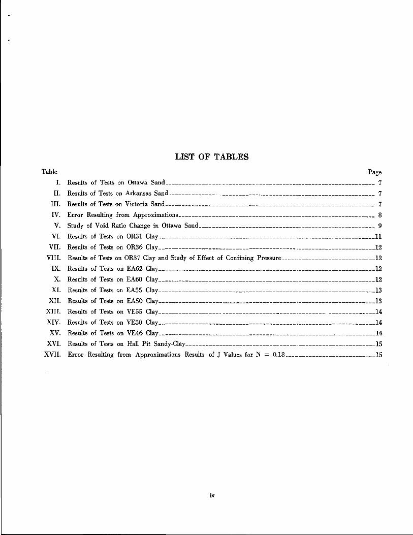
LIST OF TABLES
Table Page
I. Results of Tests on Ottawa Sand--------------------------------------------------------------- 7
II. Results of Tests on Arkansas Sand-----------------·---------------------------------------------- 7
III. Results of Tests on Victoria Sand--------------------------------------------------------------- 7
IV. Error Resulting from Approximations-----------------------------------··----------------------- 8
V. Study of Void Ratio Change in Ottawa Sand-----------------------------··----------------------- 9
VI. Results of Tests on OR31 Clay----------------------------------------- -----------------------11
VII. Results of Tests on OR36 Clay----------------------------------------- ·-----------------------12
VIII. Results of Tests on OR37 Clay and Study of Effect of Confining Pressure-----·-----------------------12
IX. Results of Tests on EA62 Clay----------------------------------------- ·-----------------------12
X. Results of Tests on EA60 Clay -----------------------------------------·-----------------------12
XL Results of Tests on EASS Clay -----------------------------------------··-----------------------13
XII. Results of Tests on EASO ClaY-----------------------------------------·-----------------------13
XIII. Results of Tests on VE55 ClaY-----------------------------------------·------------------------14
XIV. Results of Tests on VESO Clay----------------------------------------- ------------------------14
XV. Results of Tests on VE46 Clay----------------------------------------- ------------------------14
XVI. Results of Tests on Hall Pit Sandy-Clay ----------------------------·-----··-----------------------15 XVII. Error Resulting from Approximations Results of J Values for N = 0.18 ___________________________ 15
iv

LIST OF FIGURES
Figure Page
1 Soil Resistance versus Deformation Diagram for Soils ______________________________________________ 1
2 Smith's Rheological Model (after Smith)---------------------------------------------------------- 1
3 Picture of Apparatus and General Schematic Diagram of Setup------------------------------------ 3
4 The Triaxial Base Load Cell--------------------------------------------·------------------------ 3
5 Loading Apparatus-----------------------------------------------------·----------------------- 3
6 Average Velocity of Deformation versus Height of Drop--------------------------------------------- 4
7 Grain Size Curve for Sands Tested--------------------------------------------------------------- 5
8 Equipment setup for Impact Test on Ottawa Sand---------------------------------,---------------- 5
9 Velocity of Sample Deformation versus Peak Dynamic Load for Sands Tested_·----------------------- 6
10 Pdynnmic/Pstatic versus Velocity of Deformation for Sands Tested _______________________________________ 6
11 Smith's J versus Velocity of Deformation for Sands Tested---------------------------~-------------- 6
12 Damping Constant versus Velocity for Defo-rmation Raised to Optimum Power for Sands Tested ________ 7
13 Damping Constant versus Velocity of Deformation Raised to .20 Power for Sands Tested ______________ 8
14 Effective Angle of Internal Shearing Resistance versus Damping Constant for Sands Tested_____________ 8
15 Peak Dynamic Load versus Velocity of Deformation for Void Ratio Study on Ottawa Sand------------- 8
16 Void Ratio versus Damping Constant for Ottawa Sand---------------------------------------------- 9
17 Location on Plasticity Chart of Clays Tested -------------------------------------··-----------------10 18 Vetters Clay at Three Moisture Contents Before and After Failure ____________________________________ 10
19 Effect of Confining Pressure on OR 37 MateriaL_ -------------------------------------------------10 20 Effect of Sample Height on Dynamic Load in OR 36 MateriaL ______________________________________ 10
21 Dynamic Load versus Velocity of Deformation for Clays Tested ------------------------------------11
22 Ratio of Dynamic to Static Load versus Velocity of Deformation for Clays Tested ______________________ 11
23 Smith's J versus Velocity of Deformation for EA 50 MateriaL ___________________________________ 11
24 Damping Constant at N = Optimum versus Velocity of Deformation for Clays _________________________ 13
25 Damping Constant at N = 0.18 versus Velocity of Deformation for Clays Tested _____________ :_ ________ 13
26 Moisture Content versus Damping Constant for Vetters ClaY----------------------------------------14 27 Liquidity Index versus Damping Constant for Clays Tested __________________________________________ 15
A-1 Sample Visicorder Trace----------------------- -------------------------------------------------18 C-1 Method of Obtaining Velocity to Optimum Power_ __________________________________________________ 25
D-1 Mohr's Circle Diagram for Ottawa Sand ___________________________________________________________ 26
D-2 Mohr's Circle Diagram for Arkansas Sand _________________________________________________________ 27
D-3 Mohr's Circle Diagram for Victoria Sand __________________________________________________________ 28
v
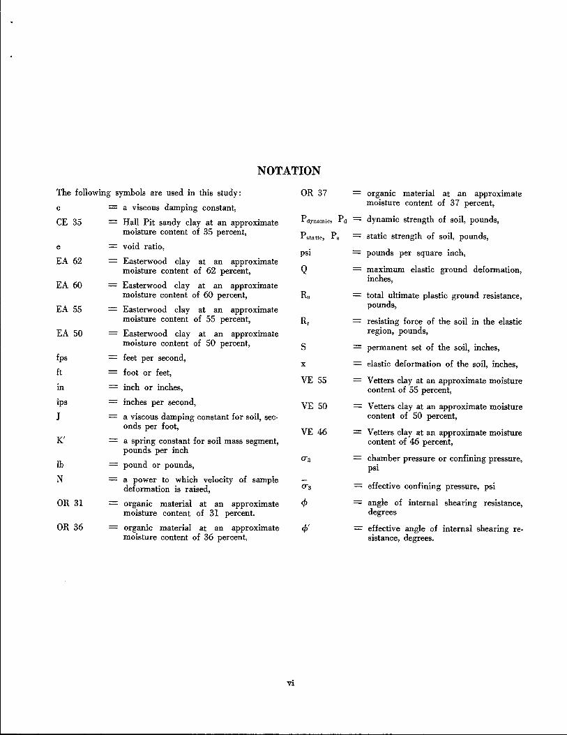
NOTATION
The following symbols are used in this study: OR 37
c a viscous damping constant,
CE 35 Hall Pit sandy clay at an approximate Pdynamic, pd
moisture content of 35 percent, P static, P. e void ratio,
psi EA 62 Easterwood clay at an approximate
moisture content of 62 percent, Q EA 60 Easterwood clay at an approximate
moisture content of 60 percent, Ru
EA 55 Easterwood clay at an approximate moisture content of 55 percent, Rr
EA 50 Easterwood clay at an approximate moisture content of 50 percent, s
fps feet per second, X
ft foot or feet, VE 55
Ill inch or inches,
ips inches per second, VE 50 J a viscous damping constant for soil, sec-
onds per foot, VE 46
K' a spring constant for soil mass segment, pounds per inch
lb pound or pounds, o-3
N a power to which velocity of sample deformation is raised, o-3
OR 31 organic material at an approximate cf> moisture content of 31 percent.
OR 36 organic material at an approximate cf>' moisture content of 36 percent,
vi
organic material at an approximate moisture content of 37 percent,
dynamic strength of soil, pounds,
static strength of soil, pounds,
pounds per square inch,
maximum elastic ground deformation, inches,
total ultimate plastic ground resistance, pounds,
resisting force of the soil in the elastic region, pounds,
permanent set of the soil, inches,
elastic deformation of the soil, inches,
Vetters clay at an approximate moisture content of 55 percent,
Vetters clay at an approximate moisture content of 50 percent,
V etters clay at an approximate moisture content of 46 percent,
chamber pressure or confining pressure, psi
effective confining pressure, psi
angle of internal shearing resistance, degrees
effective angle of internal shearing resistance, degrees.

Soil Damping Constants Related to Common Soil Properties
in Sands and Clays
CHAPTER I INTRODUCTION
Study of Dynamic Behavior of Piling
The dynamic behavior of piling has been of great concern to Civil Engineers for many years. In I962, E. A. L Smith (IO) * suggested a numerical solution to the pile driving problem. Smith presented the concept for static loading at the point of a pile such that the ground compresses elastically for a certain distance and then fails plastically with a constant resistance. This concept is illustrated in Figure l by the dotted line OABC. Q in the figure represents the maximum elastic ground deformation or "quake" and Ru represents the total ultimate plastic ground resistance to the pile. Under static loading the pile deforms the ground elastically through OA and then plastically through a distance S. The soil then rebounds from B to C leaving a permanent set of S.
E. A. L Smith (10) developed a mathematical model which accounts for both static and dynamic soil behavior. Figure 2 shows the rheological model which simulates the mathematical model proposed by Smith. The model consists of a spring and friction block in series connected in parallel to a dashpot. If the model were suddenly compressed a certain distance, the following equation would describe the soil's resistance in the elastic region (see Figure I):
*Numerals in parentheses refer to corresponding items in list of references. The citations on the following pages follow the style of the Journal of the Soil Mechanics and Foundations Division, American Society of Civil Engineers.
~ Ru.JV
Ill () z c ~ II)
SLIDING FRICTION BLOCK FOR PLASTIC DEFORMATION
SPRING FOR ELASTIC DEFORMATION
ON SOIL
DASHPOT FOR VISCOUS DAMPING
Figure 2. Smith's rheological model (after Smith).
where: Rr K'
Rr = K'x + cV
resisting force, soil spring constant,
c - a viscous damping constant,
(I)
v x - elastic deformation of the soil or "Quake,"
the instantaneous velocity of the point of the pile in any time interval.
The friction block accounts for the constant soil resistance in the plastic region during static loading and thus does not appear in equation I. In order to include the effect of the pile's size and shape Smith has made:
c = K'xJ (2)
where J is a viscous damping constant for the soil similar to c. As the velocity of deformation approaches zero in equation I, the dynamic resisting force approaches a static value:
Pstatic = K'x (3)
Ru Letting P dynamic: equal Rr in equation I from Smith's ;; Rr Ill a: ..J 0 II) 0
DEFORMATION
Figure 1. Soil resistance versus deformation diagram for soils.
mathematical model and substituting equations 2 and 3 into I, the peak dynamic resistance of the soil is:
Pd,·namic = Pstatic (I + JV) ( 4)·
Samson, Hirsch and Lowery (7, 8) expanded Smith's static loading- concept to the dynamic concept represented by line OA'BC of Figure I. If Ru in Figure I is the static soil resistance, then Ru JV is the dynamic portion of the total soil resistance.
PAGE ONE
l..,_ _____________________________________________ _
This concept for the resistance at the point of the pile takes into account:
l. elastic ground deformation,
2. ultimate ground resistance, and
3. viscous damping constant based on damping constant "J".
Smith assigned a value of J = 0.15 for use by investigators until such time that new facts were developed. He pointed out that his mathematical model could be modified to account for the new facts as they were obtained.
Smith's work was augmented by Samson, Hirsch, and Lowery (7, 8) so that the driving of a pile could be simulated by use of the digital computer. It was their feeling that the resistance to dynamic loading at the point of the pile is not clearly understood and that future study might shed more light on the problem.
Study of Dynamic Behavior of Soils
It is known that the compressive strength of a soil is a function of the time required to reach a failure load. Nishida (4) in his paper entitled "A Soil Strength Subject to Falling Impact" studied this effect and found it to be true. Hampton and Yoder (2) found that in silty clay and clay the unconfined compressive strength showed significant increases with rate of strain for all compactive efforts and all moisture contents tested. Whitman and Healy (12) did an extensive study on shear strength in sands during rapid loading. They developed techniques for applying strains rapidly and measuring resultant stresses and pore pressures and presented information concerning membrane and inertia effects in triaxial tests. Jones, Lister, and Thrower (3) in a related study presented a comprehensive literature study of the subject of dynamic loading of soils.
Chan ( 1) investigated in the laboratory the dynamic load deformation and damping properties in sands. Reeves ( 5) did laboratory research and evaluated the damping constants of sands subjected to impact loads.
Using experimental data and Smith's equation, Reeves determined that the damping constant, J, was actually a variable for a saturated sand. By modifying Smith's equation in the following manner he was able to obtain a constant J value.
Pdyuamic = Pstatic (I + JV) (5)
This modification of Smith's equation involves an intercept value, I. To evaluate this intercept, Reeves performed dynamic tests, finding the ratio of dynamic to static load versus velocity of sample deformation to be a straight line between velocities of 3-12 fps. He then extended this straight line to the P d/P s axis and obtained an intercept, I. Using this intercept in equation 5 he was able to evaluate a constant J value in the range of 3-12 fps.
Sulaiman ( ll) did a study in which he was concerned with the static side friction values encountered in various types of sand. Raba ( 6) investigated side frictional damping (J') developed in clays using a model pile in the laboratory. Raba was able to relate J' to liquidity index for CH materials.
Scope of This Study
From the foregoing discussion, it can be seen that some work has been done on pile-soil systems and evaluating damping constants for soils. With the exception of Raba's work in clays, there has been little done in relating soil damping constants to common soil properties.
Objectives of This Study
The objectives of this investigation are:
l. To determine soil damping constants for sands and clays by conducting laboratory impact tests on these soils, and
2. To correlate these soil damping constants with common soil properties such as void ratio and angle of internal shearing resistance in sands and liquidity index and moisture content in clays.
CHAPTER II
APPARATUS, INSTRUMENTATION, AND TEST PROCEDURE
General
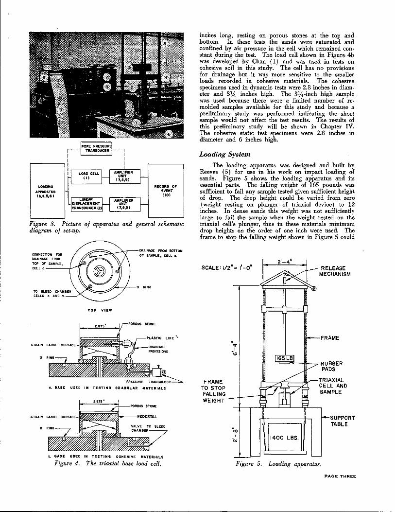
The equipment involved in this series of tests was necessarily of a special nature. In the dynamic tests it was desired to load the sample over a range of velocities from 0-12 feet per second. It was also important that a permanent record of each test be available from which the necessary calculations could be made. Figure 3 is a picture of the complete test set-up including the dynamic loading apparatus, the triaxial cell and the recording equipment. The numbers in parentheses in Figure 3 represent the location of specific items of equipment. This figure also shows a general schematic diagram of the complete apparatus in sequence of occurrence from left to right. Only general descriptions of the
PAGE TWO
equipment are given in this chapter. Detailed information can be found in a paper by Reeves ( 5) .
Triaxial Cells
Two separated triaxial devices with load cells in the base were used in this investigation. Figure 4 shows the cell bases used for both the cohesive and granular materials. The load cells consisted of SR-4 strain gages mounted on the walls of an aluminum tube or pedestal to record the compressional load on impact. The cell shown in Figure 4a was developed by Reeves ( 5) and was used in tests on san~s in this study. It has provisions for drainage of the sample at both top and bottom. All sand samples were 2.8 inches in diameter and 6
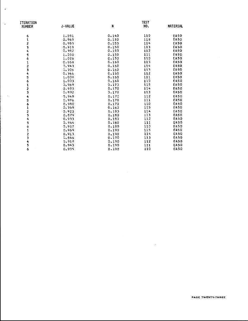
ITERATION TEST NUMBER J-VALUE N NO. MATERIAL
6 1.051 0.140 110 EA50 1 o. 969 0.150 115 EA50 2 0.953 0.150 114 EA50 3 o. 919 0.150 113 EA50 4 0.'182 0.150 112 EA50 5 1.:)30 0.150 111 EA50 6 1.026 0.150 110 EA50 1 C.969 0.160 115 EA50 2 0,943 0.160 114 EA50 3 0.'106 0.160 111 EA5'0 4 0. ·~66 0.150 112 EA50 5 1.008 0.160 111 EA50 6 1. 003 0.160 110 EA50 1 0.969 0.17':) 115 EA50 2 0.933 0.170 114 EA50 3 0.'392 0.170 113 EA50 4 0.949 0.170 112 EA50 5 0.9?6 0.170 111 EA50 6 0.9RO 0.170 110 EA50 1 0.969 0. 180 115 EA50 2 0.923 0.180 114 EA50 3 0.879 0.180 113 EA50 4 o. 933 0.18::> 112 EA50 5 0.9&4 0.180 111 EA50 6 0.957 0.180 110 EA50 1 0.969 0.190 115 EA50 2 o. 913 o. no 114 EA50 3 0.866 0.190 113 El\50 4 ').918 o. no 112 EA50 5 0.943 0.190 111 EA50 6 0.93'> 0.190 110 EA50
PAGE TWENTY-THREE
LOADING
APPARATUS \3,4,S,6)
RECORD ·oF EVENT (10)
Figure 3. Picture of apparatus and general schematic diagram of set-up.
CONNECTION FOR ORAl NAGE FROM TOP OF SAMPLE, CELL a.----f-_...-
TOP VIEW
a. BASE USED IN TESTING GRANULAR MATERIALS
b. BASE USED IN TESTING COHESIVE MATERIALS
Figure 4. The triaxial base load cell.
inches long, resting on porous stones at the top and bottom. In these tests the sands were saturated and confined by air pressure in the cell which remained constant during the test. The load cell shown in Figure 4b was developed by Chan ( 1) and was used in tests on cohesive soil in this study. The cell has no provisions for drainage but it WI!~ more sensitive to the smaller loads recorded in cohesive materials. The cohesive specimens used in dynamic tests were 2.8 inches in diameter and 314 inches high. The 314 -inch high sample was used because there were a limited number of remolded samples available for this study and because a preliminary study was performed indicating the sho-rt sample would not affect the test results. The results of this preliminary study will be shown in Chapter IV. The cohesive static test specimens were 2.8 inches in diameter and 6 inches high.
Loading System
The loading apparatus was designed and built by Reeves ( 5) for use in his work on impact loading of sands. Figure 5 shows the loading apparatus and its essential parts. The falling weight of 165 pounds wa& sufficient to fail any sample tested given sufficient height of drop. The drop height could be varied from zero (weight resting on plunger of triaxial device) to 12 inches. In dense sands this weight was not sufficiently large to fail the sample when the weight rested on the triaxial cell's plunger, thus in these materials minimum drop heights on the order of one inch were used. The frame to stop the falling weight shown in Figure 5 could
SCALE: 112" = 1' -0" RELEASE MECHANISM
FRAME
o..;..,::~c,.._~- RUBBER
FRAME TO STOP FALL lNG _...1---'l=TWEIGHT
1400 LBS.
PADS
TRIAXIAL CELL AND SAMPLE
SUPPORT TABLE
Figure 5. Loading apparatus.
PAGE THREE
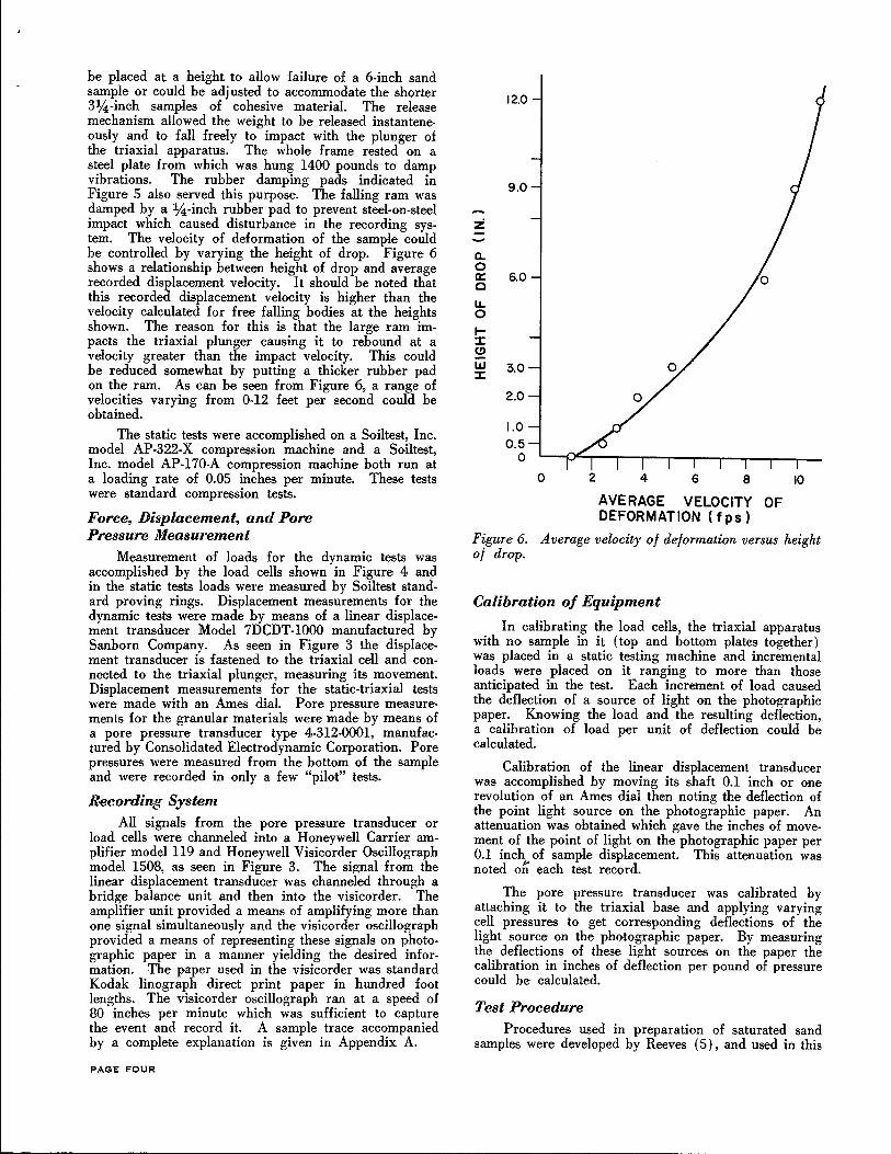
be placed at a height to allow failure of a 6-inch sand sample or could be adjusted to accommodate the shorter 3~-inch samples of cohesive material. The release mechanism allowed the weight to be released instanteneously and to fall freely to impact with the plunger of the triaxial apparatus. The whole frame rested on a steel plate from which was hung 1400 pounds to damp vibrations. The rubber damping pads indicated in Figure 5 also served this purpose. The falling ram was damped by a ~-inch rubber pad to prevent steel-on-steel impact which caused disturbance in the recording system. The velocity of deformation of the sample could be controlled by varying the height of drop. Figure 6 shows a relationship between height of drop and average recorded displacement velocity. It should be noted that this recorded displacement velocity is higher than the velocity calculated for free falling bodies at the heights shown. The reason for this is that the large ram impacts the triaxial plunger causing it to rebound at a velocity greater than the impact velocity. This could be reduced somewhat by putting a thicker rubber pad on the ram. As can be seen from Figure 6, a range of velocities varying from 0-12 feet per second could be obtained.
The static tests were accomplished on a Soiltest, Inc. model AP-322-X compression machine and a Soiltest, Inc. model AP-170-A compression machine both run at a loading rate of 0.05 inches per minute. These tests were standard compression tests.
Force, Displacement, and Pore Pressure Measurement
Measurement of loads for the dynamic tests was accomplished by the load cells shown in Figure 4 and in the static tests loads were measured by Soiltest standard proving rings. Displacement measurements for the dynamic tests were made by means of a linear displacement transducer Model 7DCDT-l000 manufactured by Sanborn Company. As seen in Figure 3 the displacement transducer is fastened to the triaxial cell and connected to the triaxial plunger, measuring its movement. Displacement measurements for the static-triaxial tests were made with an Ames dial. Pore pressure measurements for the granular materials were made by means of a pore pressure transducer type 4-312-0001, manufactured by Consolidated Electrodynamic Corporation. Pore pressures were measured from the bottom of the sample and were recorded in only a few "pilot" tests.
Recording System All signals from the pore pressure transducer or
load cells were channeled into a Honeywell Carrier amplifier model 119 and Honeywell Visicorder Oscillograph model 1508, as seen in Figure 3. The signal from the linear displacement transducer was channeled through a bridge balance unit and then into the visicorder. The amplifier unit provided a means of amplifying more than one signal simultaneously and the visicorder oscillograph provided a means of representing these signals on photographic paper in a manner yielding the desired information. The paper used in the visicorder was standard Kodak linograph direct print paper in hundred foot lengths. The visicorder oscillograph ran at a speed of 80 inches per minute which was sufficient to capture the event and record it. A sample trace accompanied by a complete explanation is given in Appendix A.
PAGE FOUR
a.. 0
12.0
9.0
a: 6.0 0
u. 0
1-:J: (!)
LLJ :I:
3.0
2.0
1.0 0.5
0
0 2 4 6 8
AVERAGE VELOCITY OF DEFORMATION ( f ps)
10
Figure 6. Average velocity of deformation versus height of drop.
Calibration of Equipment
In calibrating the load cells, the triaxial apparatus with no sample in it (top and bottom plates together) was placed in a static testing machine and incremental loads were placed on it ranging to more than those anticipated in the test. Each increment of load caused the deflection of a source of light on the photographic paper. Knowing the load and the resulting deflection, a calibration of load per unit of deflection could be calculated.
Calibration of the linear displacement transducer was accomplished by moving its shaft 0.1 inch or one revolution of an Ames dial then noting the deflection of the point light source on the photographic paper. An attenuation was obtained which gave the inches of movement of the point of light on the photographic paper per 0.1 inch of sample displacement. This attenuation was noted ori each test record.
The pore pressure transducer was calibrated by attaching it to the triaxial base and applying varying cell pressures to get corresponding deflections of the light source on the photographic paper. By measuring the deflections of these li:rht sources on the paper the calibration in inches of deflection per pound of pressure could be calculated.
Test Procedure Procedures used in preparation of saturated sand
samples were developed by Reeves ( 5), and used in this

study. The cohesive materials were tested in unconfined compression. They were remolded samples prepared by use of a V ac-aire extrusion machine, made by International Clay Machinery Company of Delaware, Model Laboratory, Serial No. A-843. Shiffert (9) did consid-
erable work with this machine and has shown that the samples produced are uniform. Raba (6) used some ~f Shiffert's samples and found them to be reliable. The samples used in this investigation were some of those prepared by Shiffert.
; CHAPTER III RESULTS OF TESTS ON SANDS
General In testing the granular materials it was desired to
get as wide a variation in physical properties as possible. A series of tests were conducted on Ottawa 20-30, Arkansas, and Victoria sands which vary in grain size and angularity of grains. Ottawa sand has uniform smooth grains; Arkansas sand has fine, angular grains; and Victoria sand has very fine and extremely angular grains. A grain size analysis is shown in Figure 7. Figure 8 shows a sample of Ottawa sand in the triaxial cell ready for impact.
It was desired to test these materials in the same manner so that comparisons of the damping constant could be made with certain properties of the sand. The dynamic tests performed were unconsolidated undrained tests, at a void ratio of 0.55, and a chamber pressure of 15 psi. Due to the method of sample preparation, the initial effective confining pressure was actually about -0.5 psi in the dynamic tests. The reason for this was that a 0.5 psi vacuum was applied during sample prepa-
a: 60 I&J z ii:
.... z ... 40 (.) a: I&J Q.
20
0 0.5 0.05
GRAIN SIZE (mm.)
Figure 7. Grain size curve for sands tested.
ration ( 5) . The static tests were performed consolidated drained, at a void ratio of 0.55 and a confining pressure of 15 psi. The dynamic tests were performed as undrained tests because at the instant of impact in driving a pile, it is felt that the water in the soil probably would not have time to drain. Conversely, the static tests were performed as drained tests because given sufficient time and a static loading the water in the soil would drain and the pore pressures would not develop.
A preliminary study was performed on Ottawa sand in which the void ratio was varied. The dynamic tests
Figure 8. Equipment set-ztp for impact test on Ottawa sand.
PAGE FIVE
were performed unconsolidated undrained, with a 15-psi chamber pressure and void ratios varying from 0.50 to 0.60. The static tests in this series were performed as
. consolidated drained tests with an effective confining pressure of 15 psi.
As mentioned in Chapter II, pore pressures were measured in the granular materials only in "pilot" tests to observe their behavior under dynamic loading. At the 0.55 void ratio pore pressure would plunge immediately upon impact to the limiting negative value ( -14.7 psi) indicating cavitation o·f the sample. The pore pressure is, of course, integrally related to the degree of saturation of the sample. Considerable care was taken to prepare a sample which was 100% saturated. It is believed that this was accomplished since when the chamber pressure was increased by 15 psi, the pore pressure likewise increased by the same amount ( -0.5 psi to 14.5 psi).
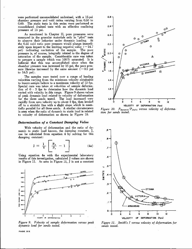
The samples were tested over a range of loading velocities varying from the minimum velocity obtainable to insure sample failure to a maximum velocity of 12 fps. Special care was taken at velocities of sample deformation of 0 - 3 fps to determine how the dynamic load varied with velocity in this range. Figure 9 shows values of peak dynamic load related to velocity of deformation for the three sands tested. The load increased very rapidly from zero velocity up to about 2 fps, then leveled off to a strai!rht line with a slight slope which is essentially parallel for all three sands. A similar circumstance is seen when the ratio of dynamic to static load is related to velocity of deformation as shown in Figure 10.
Determination of a Constant Damping Value
With velocity of deformation and the ratio of dynamic to static load known, the damping constant, J, can be calculated from equation 4 by solving for this damping constant:
1 J= v -~ -1l Ps
(4a)
- -Using equation 4a with the experimental laboratory results of this investigation, calculated J values are shown in Figure ll. As seen in Figure ll, J is not a constant
000
800
700
000
:;; = 1500 0 a .J 400
" i 300
~ 200 ~
100
10 12
VELOCITY OF DEFORMATION (fpt)
Figure 9. Velocity of sample deformation versus peak dynamic load for sands tested. .
PAGE SIX
2.8
2.6
2.4
2.2
0
~ 1- 2.0
o.UJ
~ ~ 1.8 :I!
"' z >-
o.c 1.6
1.4
1.2
1.0 0 2 4 6 8 10 12
VELOCITY OF DEFORMATION (f.ps)
Figure 10. P dyn"'mic/Pst"'tic versus velocity of deformation for sands tested.
.9
.8
.7
.6
.., .5
(/)
-~ .4 1-
:I! (/)
.3
.2
.I
0
0 2 4 6 8 10 12
VELOCITY OF DEFORMATION (fps)
Figure 11. Smith's ! versus velocity of deformaJ,ion for sands tested.
but varies with velocity o·f deformation. In order to apply Smith's wave equation analysis (10) to the piling behavior problem J must be a constant. To obtain a constant J a modification of the original Smith equation was necessary. A reasonably constant value of J was found by raising velocity of deformation to some power less than one as follows:
J = _!.__ [pd - 1l VN Ps (6)
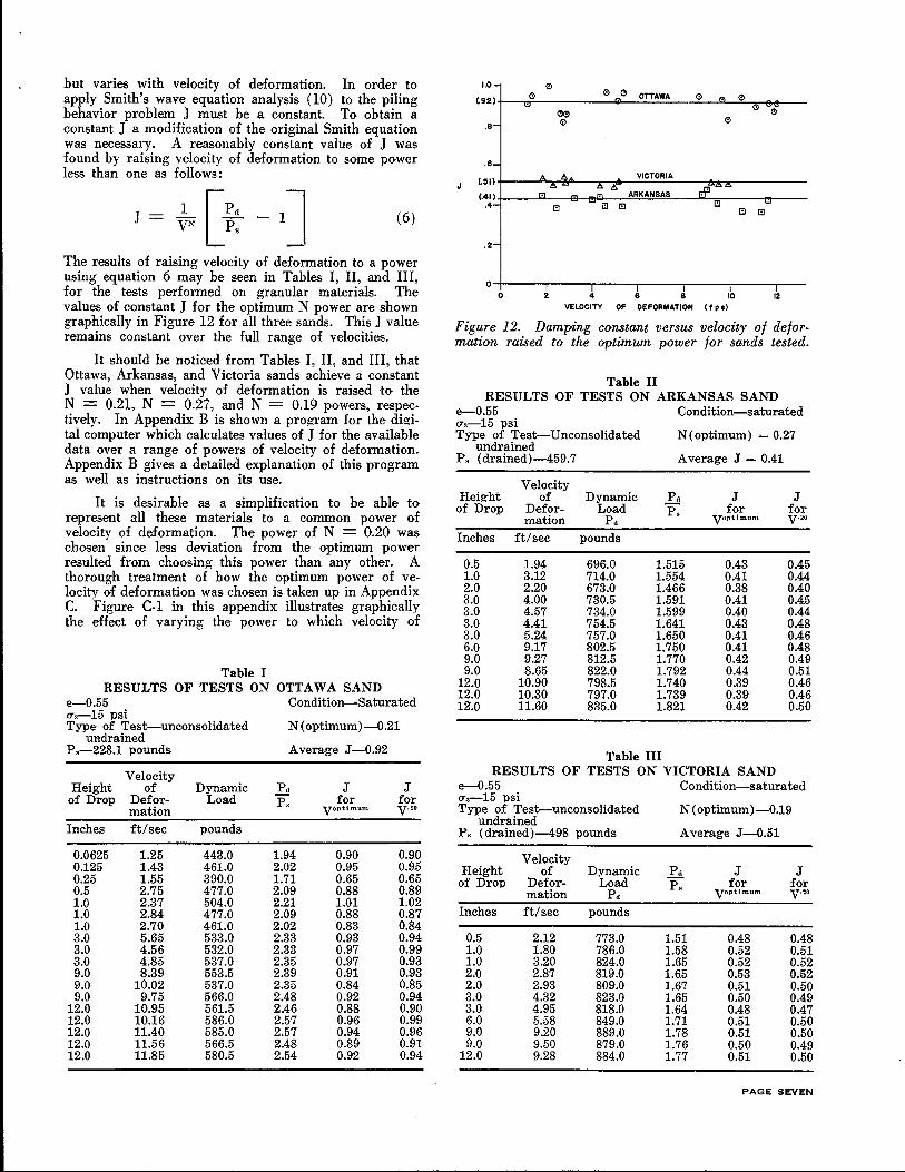
The results of raising velocity of deformation to a power using equation 6 may be seen in Tables I, II, and III, for the tests performed on granular materials. The values of constant J for the optimum N power are shown graphically in Figure 12 for all three sands. This J value remains constant over the full range of velocities.
It should be noticed from Tables I, II, and III, that Ottawa, Arkansas, and Victoria sands achieve a constant J value when velocity of deformation is raised to the N = 0.21, N = 0.27, and N = 0.19 powers, respec· tively. In Appendix B is shown a program for the di!dtal computer which calculates values of J for the available data over a range of powers of velocity of deformation. Appendix B gives a detailed explanation of this program as well as instructions on its use.
It is desirable as a simplification to be able to represent all these materials to a common power of velocity of deformation. The power of N = 0.20 was chosen since less deviation from the optimum power resulted from choosin11; this power than any other. A thorough treatment of how the optimum power of velocity of deformation was chosen is taken up in Appendix C. Figure C-1 in this appendix illustrates graphically the effect of varying the power to which velocity of
Table I RESULTS OF TESTS ON OTTAWA SAND
e-0.55 Condition-Saturated u,.--15 psi Type of Test-unconsolidated N(optimum)-0.21
undrained P ,-228.1 pounds Average J-0.92
Velocity J Height of Dynamic P,, J
of Drop Defor- Load p, for for mation voptlmum v·••
Inches ft/sec pounds
0.0625 1.25 443.0 1.94 0.90 0.90 0.125 1.43 461.0 2.02 0.95 0.9.5 0.25 1.55 390.0 1.71 0.65 0.65 0.5 2.75 477.0 2.09 0.88 0.89 1.0 2.37 504.0 2.21 1.01 1.02 1.0 2.84 477.0 2.09 0.88 0.87 1.0 2.70 461.0 2.02 0.83 0.84 3.0 5.65 533.0 2.33 0.93 0.94 3.0 4.56 532.0 2.33 0.97 0.99 3.0 4.85 537.0 2.35 0.97 0.93 9.0 8.39 553.5 2.39 0.91 0.93 9.0 10.02 537.0 2.35 0.84 0.85 9.0 9.75 566.0 2.48 0.92 0.94
12.0 10.95 561.5 2.46 0.88 0.90 12.0 10.16 586.0 2.57 0.96 0.99 12.0 11.40 585.0 2.57 0.94 0.96 12.0 11.56 566.5 2.48 0.89 0.91 12.0 11.85 580.5 2.54 0.92 0.94
.e-
.6-
(.lil) +----""'~-%& .!>-...,-..,!l-!!VIC::_:T_:::O:;::RIA:__-l!r~:------o /:> !S. ..!"'1 •• -=~
(.411+---.Jll!l•L.._--f-"'-~si.J'l.l:l:• ::---A~R~K~AN!!S_!!!AS!.__!;,!.I:J--;:;;---'fj----.4- l!l 1!1 l!l l!l l!l 1!1"'
o~--.---r---.---.---.--~--4 ~ J I~ I~ 0 2 VELOCITY OF DEFORMATION ( f p o)
Figure 12. Damping constant versus velocity of defor-mation raised to the optimum power for sands tested.
Table II RESULTS OF TESTS ON ARKANSAS SAND
e-0.55 Condition-saturated u.--15 psi Type of Test-Unconsolidated N(optimum) = 0.27
undrained P, (drained)-459.7 Average J = 0.41
Velocity Height of Dynamic E.!! J J
of Drop Defor- Load P. for for mation P. yoptimum v·••
Inches ft/sec pounds
0.5 1.94 696.0 1.515 0.43 0.45 1.0 3.12 714.0 1.554 0.41 0.44 2.0 2.20 673.0 1.466 0.38 0.40 3.0 4.00 730.5 1.591 0.41 0.4.5 3.0 4.57 734.0 1.599 0.40 0.44 3.0 4.41 754.5 1.641 0.43 0.48 3.0 5.24 757.0 1.650 0.41 0.46 6.0 9.17 802.5 1.750 0.41 0.48 9.0 9.27 812.5 1.770 0.42 0.49 9.0 8.65 822.0 1.792 0.44 0.51
12.0 10.90 798.5 1.740 0.39 0.46 12.0 10.30 797.0 1.739 0.39 0.46 12.0 11.60 835.0 1.821 0.42 0.50
Table III RESULTS OF TESTS ON VICTORIA SAND
e-0.55 Condition-saturated u,--15 psi Type of Test-unconsolidated
undrained N ( optimum)-0.19
P, (drained)-498 pounds Average J-0.51
Velocity Height of Dynamic P. J J
of Drop Defor- Load p, for for mation P. voptimum v·••
Inches ft/sec pounds
0.5 2.12 773.0 1.51 0.48 0.48 1.0 1.80 786.0 1.58 0.52 0.51 1.0 3.20 824.0 1.65 0.52 0.52 2.0 2.87 819.0 1.6.5 0.53 0.52 2.0 2.93 809.0 1.67 0.51 0.50 3.0 4.32 823.0 1.65 0.50 0.49 3.0 4.95 818.0 1.64 0.48 0.47 6.0 5.58 849.0 1.71 0.51 0.50 9.0 9.20 889.0 1.78 0.51 0.50 9.0 9.50 879.0 1.76 0.50 0.49
12.0 9.28 884.0 1.77 0.51 0.50
PAGE SEVEN
1.0-0
0 0 OTTAWA
0 0 (.94)
0 00(!) "' 0&'
0 .a-
.6- a (.!!Olf-----""'a._,f-1!:.~--;;--.;z!r-~VI~CT~O~RI~A--~>"1!1------(.46) +---e--/!:,---r.;---e=a,;;!i8'¥.J:. ~A!!!R!!!KA!!!NJ!!SA!J!S _ _:Cl!..ll r.itlJ:l:·~-!!lr--tot l'l•J._ __
[!) u l!l "' "' .4- El
.2-
0~--.---.----~----r-----r-----r--
0 2 4 6 8 10 12 VELOCITY OF DEFORMATION ( f po)
Fig~re 13.. Damping constant versus velocity of deformatwn raLSed to the .20 power for sands tested.
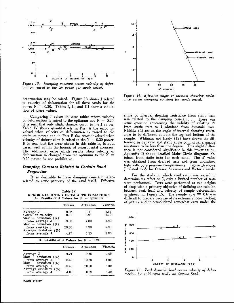
deformation may be raised. Figure 13 shows J related to velocity of deformation for all three sands for the power N = 0.20. Tables I, II, and III show a tabulation of these values.
Comparing J values in these tables where velocity of deformation is raised to the optimum and N = 0.20 it is seen that only slight changes occur in the J values: Table IV shows quantitatively in Part A the error involved when velocity of deformation is raised to the optimum power and in Part B the error involved when vel?City of deformation is raised to the N = 0.20 power. It Is seen that the error shown in this table is, in both cases, well within the bounds of experimental accuracy. The additional error which results when velocity of deformation is changed from the optimum to the N 0.20 power is not prohibitive.
Damping Constant Related to Certain Sand Properties
It is desirable to have damping constant values related to some property of the sand itself. Effective
Table IV ERROR RESULTING FROM APPROXIMATIONS
A. Results of J Values for N = optimum
Ottawa Arkansas Victoria
Average J 0.92 0.41 0.51 Power of velocity 0.21 0.27 0.19 Max + deviation (%)
from average J 9.90 7.30 3.90 Max - deviation (%)
from average J 29.50 7.30 5.90 Average deviation (%)
from average J 4.27 5.15 3.36
B. Results of J Values for N = 0.20
Ottawa Arkansas Victoria
Average J 0.94 0.46 0.50 Max + deviation (%)
from average J Max - deviation (%)
8.50 10.80 4.00
from average J Average deviation (%)
30.40 10.80 6.00
from average J 4.65 6.09 3.40
PAGE EIGHT
1.0
.8
.6
.4
0 10 20 30
'' I DEGREES )
OTTAWA SAND
ARKANSAS SAND
40 50
Figure 14. Effective angle of internal shearing resistance versus damping constant for sands tested.
angle of internal shearing resistance from static tests was related to the damping constant, J. There was some qu~tion concerning t~e validity of relating cp' fr?m. static tests to J obtamed from dynamic tests. NIshida ( 4) . shows the angle of internal shearin 0" resistance to be different at both the t~p and botto~ of the sample. Whitman and Healy (12) have shown the difference in dynamic and static angle of internal shearinoresistance to be less than one degree. This slicrht diffe; ence is not considered significant in this inv~tio-ation. Appendix D shows detailed Mohr Circle diagra!s obtained from static tests for each sand. The cp' value was obtained from drained tests and from undrained tests with pore pressure measurements. Figure 14 shows J related to cp' for Ottawa, Arkansas and Victoria sands.
For the study in which void ratio was varied to determine its effect on J, only a limited number of tests were performed. Tests were performed at two heicrhts of drop with a primary objective of defining the relafion between peak load and velocity of sample deformation as shown in Figure 15. The sample at e = 0.6 was difficult to prepare because of its extremely loose packing of grains and it consolidated somewhat even under the
1000
~ 800 I: .!I
0 c g 600
() •= .6 i c 400 z ,. 0
X 200 c .. Q.
0 2 4 6 8
VELOCITY OF DEFORMATION (F. P.S.)
Figure 15. Peak dynamic load versus velocity of deformation for void ratio study on Ottawa Sand.
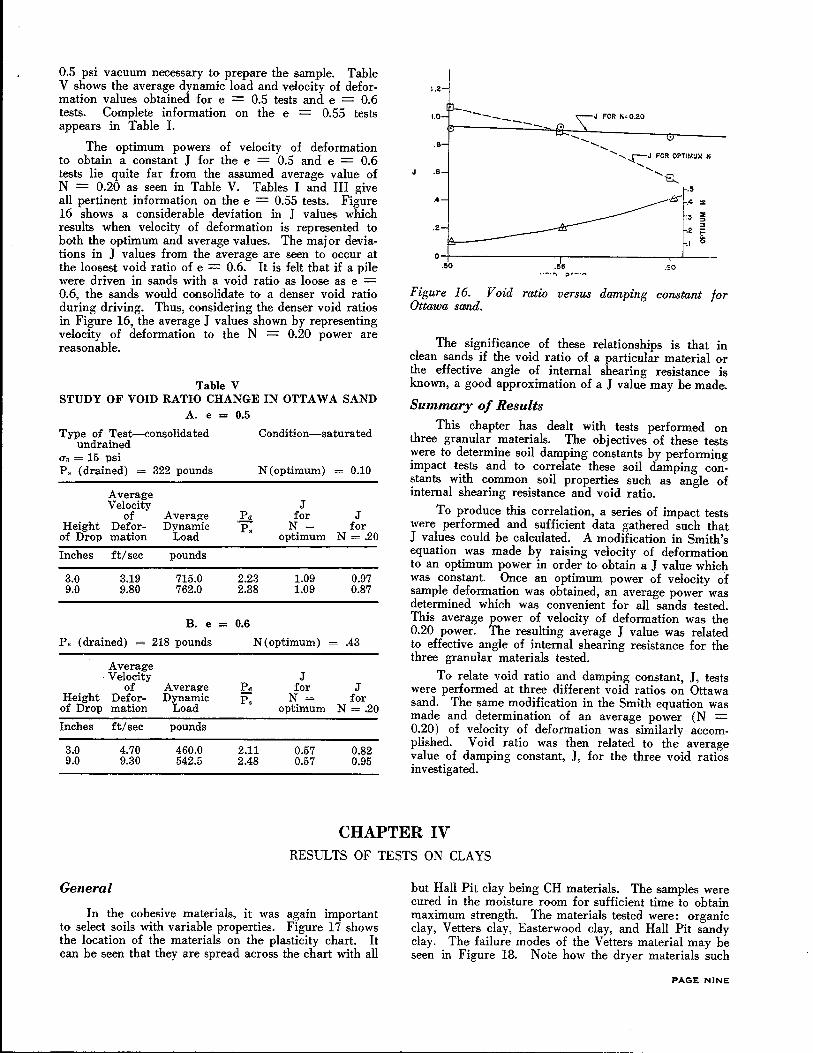
0.5 psi vacuum necessary to prepare the sample. Table V shows the average dynamic load and velocity of deformation values obtained for e = 0.5 tests and e = 0.6 tests. Complete information on the e = 0.55 tests appears in Table I.
The optimum powers of velocity of deformation to obtain a constant J for the e = 0.5 and e = 0.6 tests lie quite far from the assumed average value of N = 0.20 as seen in Table V. Tables I and III give all pertinent information on the e = 0.55 tests. Figure 16 shows a considerable deviation in J values which results when velocity of deformation is represented to both the optimum and average values. The major deviations in J values from the average are seen to occur at the loosest void ratio of e = 0.6. It is felt that if a pile were driven in sands with a void ratio as loose as e = 0.6, the sands would consolidate to a denser void ratio during driving. Thus, considering the denser void ratios in Figure 16, the average J values shown by representing velocity of deformation to the N = 0.20 power are reasonable.
Table V STUDY OF VOID RATIO CHANGE IN OTTAWA SAND
A. e = 0.5
Type of Test-consolidated Condition-saturated undrained
Us= 15 psi P, (drained) = 322 pounds N(optimum) 0.10
Average J Velocity
of Averag-e p" for J Height Defor- Dynamic 'P: N= for
of Drop mation Load optimum N = .20
Inches ft/sec pounds
3.0 3.19 715.0 2.23 1.09 0.97 9.0 9.80 762.0 2.38 1.09 0.87
B. e = 0.6
P. (drained) = 218 pounds N(optimum) .43
Average . Velocity J
of Average P. for J Height Defor- Dynamic P. N= for of Drop mation Load optimum N = .20
Inches ft/sec pounds
3.0 4.70 460.0 2.11 0.57 0.82 9.0 9.30 542.5 2.48 0.57 0.95
1.2
1.0
.8 ----
.6
.4
.2
0 .so
~ FOR N•0.20
-- ..... '......_~~FOR OPTIMUM N
'B... .5
-6.' .~ "'
.3 ~ :l!
.2 t
.I o
.$0
Figure 16. Void ratio versus damping constant for Ottawa sand.
The significance of these relationships is that in clean sands if the void ratio of a particular material or the effective angle of internal shearing resistance is known, a good approximation of a J value may be made.
Summary of Results
This chapter has dealt with tests performed on three granular materials. The objectives of these tests were to determine soil damping constants by performing impact tests and to correlate these soil damping constants with common soil properties such as angle of internal shearing resistance and void ratio.
To produce this correlation, a series of impact tests were performed and sufficient data gathered such that J values could be calculated. A modification in Smith's equation was made by raising velocity of deformation to an optimum power in order to obtain a J value which was constant. Once an optimum power of velocity of sample defo-rmation was obtained, an average power was determined which was convenient for all sands tested. This average power of velocity of deformation was the 0.20 power. The resulting average J value was related to effective angle of internal shearing resistance for the three granular materials tested.
To relate void ratio and damping constant, J, tests were performed at three different void ratios on Ottawa sand. The same modification in the Smith equation was made and determination of an average power (N = 0.20) of velocity of deformation was similarly accomplished. Void ratio was then related to the average value of damping constant, J, for the three void ratios investigated.
CHAPTER IV RESULTS OF TESTS ON CLAYS
General
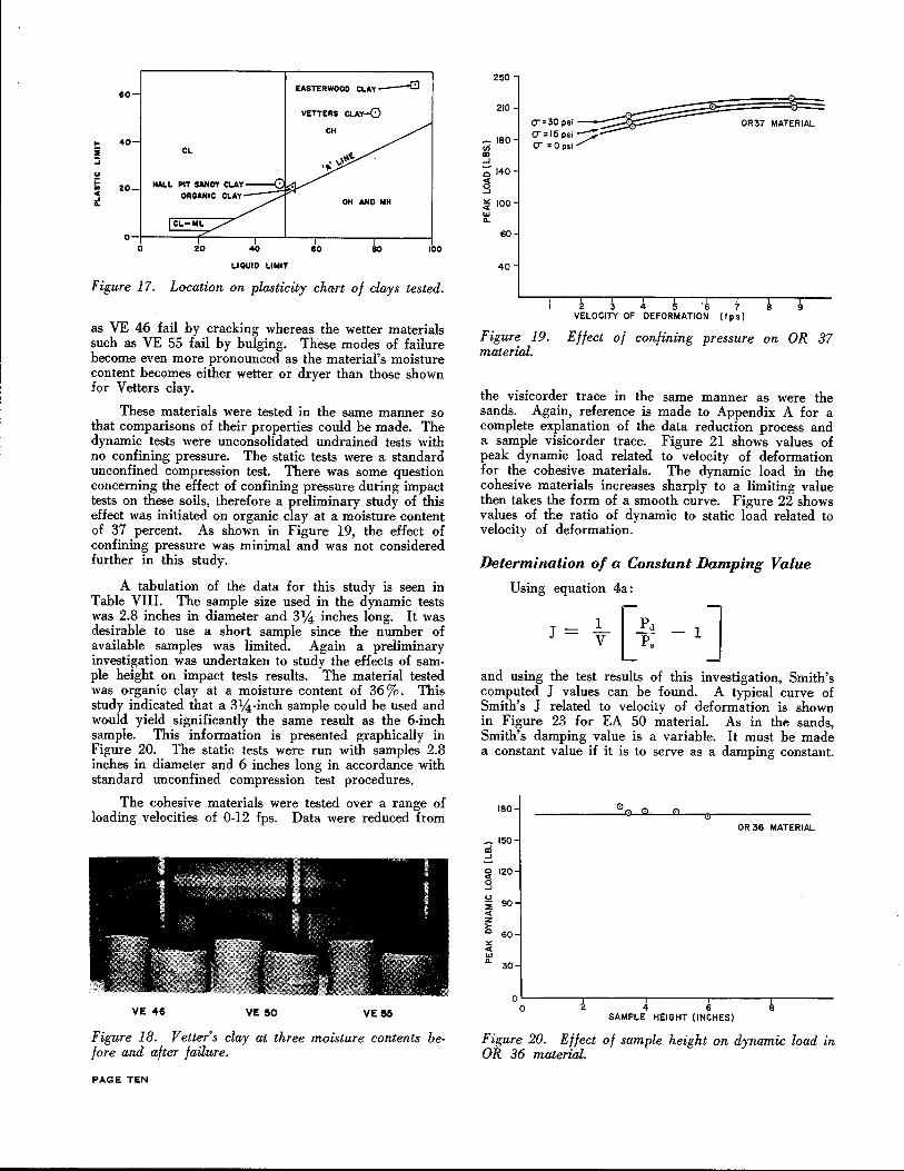
In the cohesive materials, it was again important to select soils with variable properties. Figure 17 shows the location of the materials on the plasticity chart. It can be seen that they are spread across the chart with all
but Hall Pit clay being CH materials. The samples were cured in the moisture room for sufficient time to obtain maximum strength. The materials tested were: organic clay, Vetters clay, Easterwood clay, and Hall Pit sandy clay. The failure modes of the Vetters material may be seen in Figure 18. Note how the dryer materials such
PAGE NINE
so- EASTERWOOD CLAY ---r::J
VETTERS CLAY-0
... 40 i :::; u ;::
20-.. c E
o-0 20 40
LIQUID LIMIT
Figure 17. Location on plasticity chart of clays tested.
as VE 46 fail by cracking whereas the wetter materials such as VE 55 fail by bulging. These modes of failure become even more pronounced as the material's moisture content becomes either wetter or dryer than those shown for Vetters clay.
These materials were tested in the same manner so that comparisons of their properties could be made. The dynamic tests were unconsolidated undrained tests with no confining pressure. The static tests were a standard unconfined compression test. There was some question concerning the effect of confining pressure during impact tests on these soils, therefore a preliminary study of this effect was initiated on organic clay at a moisture content of 37 percent. As shown in Figure 19, the effect of confining pressure was minimal and was not considered further in this study.
A tabulation of the data for this study is seen in Table VIII. The sample size used in the dynamic tests was 2.8 inches in diameter and 3:14 inches long. It was desirable to use a short sample since the number of available samples was limited. Again a preliminary investigation was undertaken to study the effects of sample height on impact tests results. The material tested was organic clay at a moisture content of 36%. This study indicated that a 31;{.,-inch sample could be used and would yield significantly the same result as the 6-inch sample. This information is presented g-raphically in Figure 20. The static tests were run with samples 2.8 inches in diameter and 6 inches long in accordance with standard unconfined compression test procedures.
The cohesive materials were tested over a range of loading velocities of 0-12 fps. Data were reduced from
VE 46 VE 50 VE 55
Figure 18. Vetter's clay at three moisture contents before and after failure.
PAGE TEN
250
210
-180 u; CD ..J
;; 140 <(
g ~ 100
"' a..
60
40
OR37 MATERIAL
2 3 4 '6 7 9 VELOCITY OF DEFORMATION (Ips)
Figure 19. Effect of confining pressure on OR 37 material.
the visicorder trace in the same manner as were the sands. Again, reference is made to Appendix A for a complete explanation of the data reduction process and a sample visicorder trace. Figure 21 shows values of peak dynamic load related to velocity of deformation for the cohesive materials. The dynamic load in the cohesive materials increases sharply to a limiting value then takes the form of a smooth curve. Figure 22 shows values of the ratio of dynamic to static load related to velocity of deformation.
Determination of a Constant Damping Value
Using equation 4a:
J _!_[Pd -l] V P.
and using the test results of this investigation, Smith's computed J values can he found. A typical curve of Smith's J related to velocity of deformation is shown in Figure 23 for EA 50 material. As in the sands, Smith's damping value is a variable. It must he made a constant value if it is to serve as a damping constant.
180
-150 a:i ..J
~ 120
~ 90 <( z l5 60
" <(
"' a.. 30
0
OR 36 MATERIAL
oL------,------~-------r------.--------0 4 6 8
SAMPLE HEIGHT (INCHES)
Figure 20. Effect of sample height on dynamic load in OR 36 material.
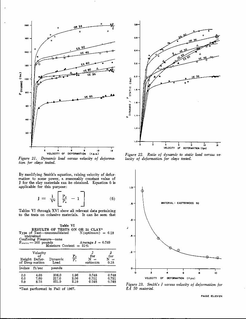
180 ~
110
140
120
.,; ~
100 u i < z > Q eo
Q.
60
40
20
2 4 6 e 10 12
VELOCITY OF DEFORMATION (f.p.s.)
Figure 21. Dynamic load versus velocity of deforrnar tion for clays tested.
By modifying Smith's equation, raising velocity of deformation to some power, a reasonably constant value of J for the clay materials can be obtained. Equation 6 is applicable for this purpose:
J ~.[ ~: - 1 J ( 6)
Tables VI through XVI show all relevant data pertaining to the tests on cohesive materials. It can be seen that
Table VI RESULTS OF TESTS ON OR 31 CLAY*
Type of Test-unconsolidated N(optimum) = 0.18 undrained
Confining Pressure-none p static- 105 pounds
Moisture Content
Velocity of pd
Height Defor- Dynamic P. of Drop mation Load
Inches ft/sec pounds
3.0 4.05 206.0 1.96 6.0 7.00 217.0 2.06 9.0 8.75 221.0 2.10
*Test performed in Fall of 1967.
Average J = 0.749 31%
J J for for
N= N= optimum 0.18
0.748 0.748 0.751 0.751 0.748 0.748
2.8
2.6
2.4
2.2
2.0 . :!
~ 1.8 ...
< ... (f)
Cl.
..... 1.6 <.>
i < z ,_ Q 1.4
Cl.
1.2
·1.0
0 4 6 8 10 12
VELOCITY OF DEFORMATION (fps)
Figure 22. Ratio of dynamic to static load versus ve· locity of deformation for clays tested.
1.0
.8 MATERIAL : EASTERWOOD 50
.6
.4
.2
0 2 4 6 8 10
VELOCITY OF DEFORMATION ( f p s)
Figure 23. Smith's ! versus velocity of deformation for EA 50 material.
PAGE ELEVEN
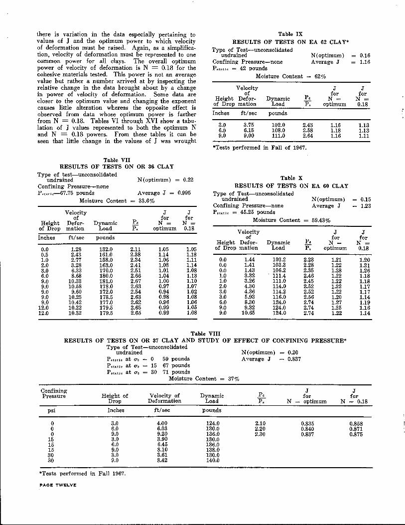
there is variation in the data especially pertaining to values of J and the optimum power to which velocity of deformation must be raised. Again, as a simplification, velocity of deformation must be represented to one common power for all clays. The overall optimum power of velocity of deformation is N = 0.18 for the cohesive materials tested. This power is not an average value but rather a number arrived at by inspecting the relative change in the data brought about by a change in power of velocity of deformation. Some data are closer to the optimum value and changing the exponent causes little alteration wl:ereas the opposite effect is observed from data whose optimum power is farther from N = 0.18. Tables VI through XVI show a tabulation of J values represented to both the optimum N and N = 0.18 powers. From these tables it can be seen that little change in the values of J was wrought
Table VII RESULTS OF TESTS ON OR 36 CLAY
Type of test-unconsolidated undrained N(optimum) = 0.22
Confining Pressure-none P,.,.,..-67.75 pounds Average J = 0.995
Moisture Content = 33.6%
Velocity J J of
P. for for
Height Defor- Dynamic N= N= of Drop mation Load P. optimum 0.18
Inches ft/sec pounds
0.0 1.28 132.0 2.11 1.05 1.05 0.5 2.43 161.0 2.38 1.14 1.18 1.0 2.77 158.0 2.34 1.06 1.11 2.0 3.28 163.0 2.41 1.08 1.14 3.0 6.33 170.0 2.51 1.01 1.08 6.0 8.68 180.0 2.66 1.04 1.13 9.0 10.33 181.0 2.67 1.00 1.10 9.0 10.58 178.0 2.63 0.97 1.07 9.0 9.60 172.0 2.54 0.94 1.02 9.0 10.25 178.5 2.63 0.98 1.08 9.0 1o.42 177.0 2.62 0.96 1.06
12.0 10.22 179.5 2.65 0.99 1.05 12.0 10.32 179.5 2.65 0.99 1.08
Table IX RESULTS OF TESTS ON EA 62 CLAY*
Type of Test-unconsolidated undrained
Confining Pressure-none P.t .. ttc = 42 pounds
N(optimum) Average J
Moisture Content = 62 o/o
Velocity J of
P. for
Height Defor- Dynamic N= of Drop mation Load p, optimum
Inches ft/sec pounds
3.0 3.75 102.0 2.43 1.16 6.0 6.15 108.0 2.58 1.18 9.0 9.00 111.0 2.64 1.16
*Tests performed in Fall of 1967.
Table X RESULTS OF TESTS ON EA 60 CLAY
Type of Test-unconsolidated undrained N(optimum)
Confining Pressure-none Average J Pstattc = 45.25 pounds
Moisture Content .59.43%
Velocity J of for
Height Defor- Dynamic P. N= of Drop mation Load P, optimum
0.0 1.44 103.2 2.28 1.21 0.0 1.41 103.3 2.28 1.22 o.o 1.43 106.2 2.35 1.28 1.0 3.32 111.4 2.46 1.22 1.0 3.26 111.0 2.45 1.22 2.0 4.30 114.0 2.52 1.22 3.0 4.36 114.2 2.52 1.22 3.0 5.93 116.0 2.56 1.20 6.0 8.30 124.0 2.74 1.27 9.0 9.32 124.0 2.74 1.25 9.0 10.65 124.0 2.74 1.22
Table VIII RESULTS OF TESTS ON OR 37 CLAY AND STUDY OF EFFECT OF CONFINING PRESSURE*
Confining Pressure
psi
0 0 0
15 15 15 30 30
Type of Test-unconsolidated undrained
P ... ,.. at ua 0 59 pounds P, .. ,.. at ua 15 67 pounds P,,,.,.. at u. 30 71 pounds
Moisture Content
Velocity of Dynamic Height of Drop Deformation Load
Inches ft/sec pounds
3.0 4.00 124.0 6.0 6.03 130.0 9.0 9.20 136.0 3.0 3.90 130.0 6.0 6.45 136.0 9.0 8.10 138.0 3.0 3.61 130.0 9.0 8.42 140.0
*Tests performed in Fall 1967.
PAGE TWELVE
37%
N(optimum) Average J
P. p,
2.10 2.20 2.30
0.20 = 0.837
J for
N = optimum
0.835 0.840 0.837
N
J
0.16 1.16
J for
N= 0.18
1.13 1.13 1.11
0.15 1.23
J for
N= 0.18
1.20 1.21 1.26 1.18 1.18 1.17 1.17 1.14 1.19 1.16 1.14
for = 0.18
0.858 0.871 0.875
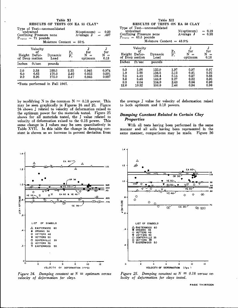
Table XI RESULTS OF TESTS ON EA 55 CLAY*
Type of Test-unconsolidated undrained N(optimum) 0.20
Confining Pressure none Average J .497 Pstnttc = 71 pounds
Moisture Content 55%
Velocity J J of P. for for
Height Defor- Dynamic P. N= N= of Drop mation Load optimum 0.18
Inches ft/sec pounds
3.0 3.58 158.0 2.23 0.945 0.974 6.0 6.65 170.0 2.40 0.955 0.991 9.0 8.95 175.0 2.47 0.945 0.987
*Tests performed in Fall 1967.
by modifying N to the common N = 0.18 power. This may be seen graphically in Figures 24 and 25. Figure 24 shows J related to velocity of deformation raised to the optimum power for the materials tested. Figure 25 shows for all materials tested, the J value related to velocity of deformation raised to the 0.18 power. This same change in J values may be seen quantitatively in Table XVII. In this table the change in damping constant is shown as an increase in percent deviation from
1.4
8 1.23
1.2
•
1.0 .995 .955 .93
~ .825 ~.e ;::: .775 0.. 0
~ ., .6
LIST OF SYMBOLS
8 EASTERWOOD 60 .4 • ORGANIC 36
0 VETTERS 46 T VETTERS 50 0 CENTERVILLE 35 G VETTERS 55
.2. 9 EASTERWOOD 50
0o~----,2----~4------6~----,e----~~o------~~2-
VELOCITY OF DEFORMATION ( F P S)
Figure 24. Damping constant at N = optimum versus velocity of deformation for clays.
Table XII RESULTS OF TESTS ON EA 50 CLAY
Type of Test-unconsolidated undrained N(optimum) 0.19
Confining Pressure none Average J 0.93 P"•"• = 63.5 pounds
Moisture Content 48.9%
Velocity J J of P. for for
Height Defor- Dynamic P. N= N= of Drop mation Load optimum 0.18 Inches ft/sec pounds
0.0 1.00 125.0 1.97 0.97 0.97 1.0 2.90 134.5 2.12 0.91 0.92 2.0 4.40 136.4 2.15 0.87 0.88 3.0 .5.48 144.0 2.27 0.92 0.93 9.0 9.04 154.0 2.43 0.94 0.96
12.0 10.32 156.0 2.46 0.94 0.96
the average J value fo·r velocity of deformation raised to both optimum and 0.18 powers.
Damping Constant Related to Certain Clay Properties
With all tests having been performed in the same manner and all soils having been represented in the same manner, comparisons may be made. Figure 26
1.4
8 1.2 II,? • • - EA6~
1.18
OR 36_.. ~, 1.09
• VE 50-....
, " 1.0 T .99
08' 0 T = T EA5Q-.... T ~ G 9 .94
9"' 0 VE55/ 0.93 1>. "' 9=
VE 46./ .88
0 0 ~ .8 0
~ 0
0 (.) 0 0 CE 35./
.70 II Q) Q) 008 !;. ., .6
LIST OF SYMBOLS:
.4 8 EASTERWOOD 60 e ORGANIC 36 0 VETTERS 45 T VETTERS 50 0 CENTERVILLE 35 G VETTERS 55 9 EASTERWOOD 50
.2
0 2 4 8 10 12
VELOCITY OF DEFORMATION (fps 1
Figure 25. Damping constant at N - 0.18 versus velocity of deformation for clays tested.
PAGE THIRTEEN
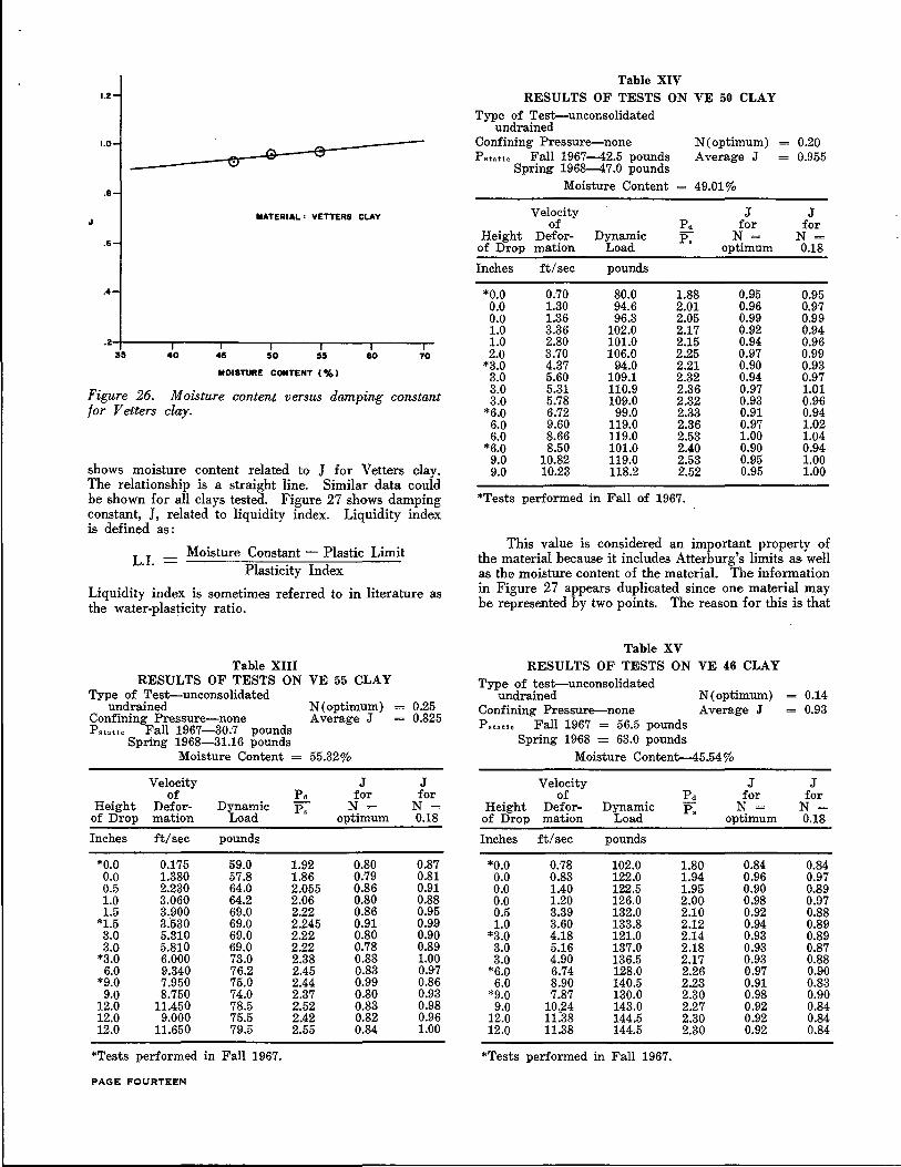
1.2
1.0 0
.8
MATERIAL ' VETTERS CLAY
.6
.4
.2-t----.---.---,.-----.---..---T"" 35 40 45 50 55 60 70
MOISTURE CONTENT (%)
Figure 26. Moisture content versus damping constant for V etters clay.
shows moisture content related to J for Vetters clay. The relationship is a straight line. Similar data could he shown for all clays tested. Figure 27 shows damping constant, J, related to liquidity index. Liquidity index is defined as :
L I = Moisture Constant - Plastic Limit · · Plasticity Index
Liquidity index is sometimes referred to in literature as the water-plasticity ratio.
Table XIII RESULTS OF TESTS ON VE 55 CLAY
Type of Test-unconsolidated undrained N(optimum) 0.25
Confining Pressure-none Average J 0.825 Pstatlc Fall 1967-30.7 pounds
Spring 1968-31.16 pounds Moisture Content 55.32%
Velocity J J of P. for for
Height Defor- Dynamic P. N= N= of Drop mation Load optimum 0.18
Inches ft/sec pounds
*0.0 0.175 59.0 1.92 0.80 0.87 o.o 1.380 57.8 1.86 0.79 0.81 0.5 2.230 64.0 2.055 0.86 0.91 1.0 3.060 64.2 2.06 0.80 0.88 1.5 3.900 69.0 2.22 0.86 0.95
*1.5 3:530 69.0 2.245 0.91 0.99 3.0 5.310 69.0 2.22 0.80 0.90 3.0 5.810 69.0 2.22 0.78 0.89
*3.0 6.000 73.0 2.38 0.88 1.00 6.0 9.340 76.2 2.45 0.83 0.97
*9.0 7.950 75.0 2.44 0.99 0.86 9.0 8.750 74.0 2.37 0.80 0.93
12.0 11.450 78.5 2.52 0.83 0.98 12.0 9.000 75.5 2.42 0.82 0.96 12.0 11.650 79.5 2.55 0.84 1.00
*Tests performed in Fall 1967.
PAGE FOURTEEN
Table XIV RESULTS OF TESTS ON VE 50 CLAY
Type of Test-unconsolidated undrained
Confining Pressure-none N(optimum) P static Fall 1967-42.5 pounds Average J
Spring 1968-47.0 pounds Moisture Content 49.01%
Velocity J of P. for
Height Defor- Dynamic P. N = of Drop mation Load optimum
Inches ft/sec pounds
*0.0 0.70 80.0 1.88 0.9.5 0.0 1.30 94.6 2.01 0.96 o.o 1.36 96.3 2.05 0.99 1.0 3.36 102.0 2.17 0.92 1.0 2.80 101.0 2.15 0.94 2.0 3.70 106.0 2.25 0.97
*3.0 4.37 94.0 2.21 0.90 3.0 5.60 109.1 2.32 0.94 3.0 5.31 110.9 2.36 0.97 3.0 5.78 109.0 2.32 0.93
*6.0 6.72 99.0 2.33 0.91 6.0 9.60 119.0 2.36 0.97 6.0 8.66 119.0 2.53 1.00
*6.0 8.50 101.0 2.40 0.90 9.0 10.82 119.0 2.53 0.95 9.0 10.23 118.2 2.52 0.95
*Tests performed in Fall of 1967.
0.20 0.955
J for
N= 0.18
0.95 0.97 0.99 0.94 0.96 0.99 0.93 0.97 1.01 0.96 0.94 1.02 1.04 0.94 1.00 1.00
This value is considered an important property of the material because it includes Atterhurg's limits as well as the moisture content of the material. The information in Figure 27 appears duplicated since one material may he represented by two points. The reason for this is that
Table XV RESULTS OF TESTS ON VE 46 CLAY
Type of test-unconsolidated undrained
Confining Pressure-none N(optimum) Average J
Pstatte Fall 1967 = 56.5 pounds Spring 1968 = 63.0 pounds
Moisture Content-45.54%
Velocity of P.
Height Defor- Dynamic
J for
N = of Drop mation Load
P. optimum
Inches ft/sec pounds
*0.0 0.78 102.0 1.80 0.84 0.0 0.83 122.0 1.94 0.96 0.0 1.40 122.5 1.95 0.90 o.o 1.20 126.0 2.00 0.98 0.5 3.39 132.0 2.10 0.92 1.0 3.60 133.8 2.12 0.94
*3.0 4.18 121.0 2.14 0.93 3.0 5.16 137.0 2.18 0.93 3.0 4.90 136.5 2.17 0.93
*6.0 6.74 128.0 2.26 0.97 6.0 8.90 140.5 2.23 0.91
*9.0 7.87 130.0 2.30 0.98 9.0 10.24 143.0 2.27 0.92
12.0 11.38 144.5 2.30 0.92 12.0 11.38 144.5 2.30 0.92
*Tests performed in Fall 1967.
0.14 0.93
J for
N= 0.18
0.84 0.97 0.89 0.97 0.88 0.89 0.89 0.87 0.88 0.90 0.83 0.90 0.84 0.84 0.84
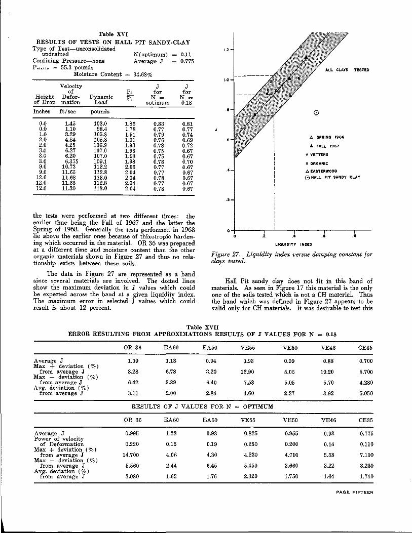
Table XVI RESULTS OF TESTS ON HALL PIT SANDY-CLAY
Type of Test-unconsolidated undrained N(optimum) 0.11
Confining Pressure-none Average J = 0.775 Pstntlc = 55.3 pounds
Moisture Content 34.68%
Velocity J J of P. for for
Height Defor- Dynamic P. N= N= of Dr9p mation Load optimum 0.18
Inches ft/sec pounds
0.0 1.45 103.0 1.86 0.83 0.81 0.0 1.10 98.4 1.78 0.77 0.77 1.0 3.29 105.8 1.91 0.79 0.74 2.0 4.84 105.8 1.91 0.76 0.69 2.0 4.25 106.9 1.93 0.78 0.72 3.0 6.27 107.0 1.93 0.75 0.67 3.0 6.20 107.0 1.93 0.75 0.67 3.0 6.375 109.1 1.98 0.78 0.70 9.0 10.73 112.2 2.03 0.77 0.67 9.0 11.65 112.8 2.04 0.77 0.67
12.0 11.68 113.0 2.04 0.78 0.67 12.0 11.65 112.8 2.04 0.77 0.67 12.0 11.30 113.0 2.04 0.78 0.67
the tests were performed at two different times: the earlier time being the Fall of 1967 and the latter the Spring of 1968. Generally the tests performed in 1968 lie above the earlier ones because of thixotropic hardening which occurred in the material. OR 36 was prepared at a different time and moisture content than the other organic materials shown in Figure 27 and thus no relationship exists between these soils.
The data in Figure 27 are represented as a band since several materials are involved. The dotted lines show the maximum deviation in J values which could be expected across the band at a given liquidity index. The maximum error in selected J values which could result is about 12 percent.
1.2
ALL CLAYS TESTED
1.0
.8 0
.6 /!;. SPRING 1968
4 FALL 1967
o VETTERS
a ORGANIC
.4 /!;. EASTERWOOD
0 HALL PIT SANDY CLAY
.2
LIQUIDITY INDEX
Figure 27. Liquidity index versus damping constant for clmys tested.
Hall Pit sandy clay does not fit in this band of materials. As seen in Figure 17 this material is the only one of the soils tested which is not a CH material. Thus the band which was defined in Figure 27 appears to be valid only for CH materials. It was desirable to test this
Table XVII ERROR RESULTING FROM APPROXIMATIONS RESULTS OF J VALUES FOR N = 0.18
OR 36 EA60 EA50 VE55 VE50 VE46 CE35
Average J 1.09 1.18 0.94 0.93 0.99 0.88 0.700 Max + deviation (%)
from average J 8.28 6.78 3.20 12.90 5.05 10.20 5.700 Max - deviation (%)
from average J A vg. deviation (%)
6.42 3.39 6.40 7.53 5.0.5 5.70 4.280
from average J 3.11 2.00 2.84 4.60 2.27 3.92 5.050
RESULTS OF J VALUES FOR N OPTIMUM
OR 36 EA60 EA50 VE55 VE50 VE46 CE35
Average J 0.995 1.23 0.93 0.825 0.955 0.93 0.775 Power of velocity
of Deformation 0.220 0.15 0.19 0.250 0.200 0.14 0.110 Max + deviation ( %)
from average J Max - deviation (%)
14.700 4.06 4.30 4.230 4.710 5.38 7.100
from average J 5.560 2.44 6.45 5.450 3.660 3.22 3.230 Avg. deviation (%)
from average J 3.080 1.62 1.76 2.320 1.750 1.64 1.740
PAGE FIFTEEN
material in <>rder t<> define the b<>undaries <>f the relati<>nships obtained. The band of Figure 27 likely defines the band of CH materials since the soils which lie in it are well spread across the CH p<>rti<>n of the plasticity chart.
The significance of these relationships are that if certain pmperties <>f the material are kn<>wn such as m<>isture c<>ntent and Atterburg limits, a good approximation of J value can be made.
Summary of Results
This chapter dealt with tests performed on organic clay, Easterwo<>d clay, Vetters clay and Hall Pit sandy clay. The <>bjectives of these tests were to determine
soil damping constants related to soil properties such as moisture content and liquidity index.
To correlate moisture content and liquidity index with the damping constant, J, a series of impact tests were performed and sufficient data gathered to calculate J values. As in the sand tests, Smith's J value varied with velocity of deformation. It was necessary to modify Smith's equation by raising velocity of deformation to a power in order to make J a constant. This optimum power differed for each clay but all materials tested could be represented to the 0.18 power without excessive error.
Moisture content was then related to damping constant, J, for Vetters clay. Liquidity index was related to J for all CH materials tested.
CHAPTER V CONCLUSIONS
The conclusions drawn from this investigation are:
l. Based on applying the experimental laboratory data of this study to Smith's equation, Smith's J value varies with velocity of deformation for the materials tested.
2. Reeves' intercept method of modifying Smith's equation is valid only between loading velocities of 3-12 fps in sands and does not account for the initial portion of the load versus velocity of deformation curve.
3. Smith's equation can be modified to make J a constant for all values of load and velocity of deformation from 0-12 fps.
4. An acceptable constant J value for a clean sand may be obtained by raising velocity of deformation to the 0.20 power.
5. An acceptable constant J value for a highly_ plas-
tic clay may be obtained by raising velocity of deformation to the 0.18 power.
6. An approximate J value may be obtained:
a. For a particular clean sand if its void ratio is known.
b. For any clean sand if its effective angle of internal shearing resistance is known.
7. An approximate J value may be obtained:
a. In a particular highly plastic clay if its moisture content is known.
b. In any highly plastic clay if its liquidity index is known.
8. Other bands of data are believed to exist for materials other than clean sands and highly plastic clays based on tests performed on Hall Pit sandy clay.
CHAPTER VI RECOMMENDATIONS
This investigation is a beginning in relating common properties of soils to a damping constant. Similar tests on <>ther soils could shed light on J values for other materials such as silts and materials of low plasticity and could more specifically define the data obtained in this investigation. At the conclusion of a similar study, values of J could probably be approximated for most soils so that a more accurate analysis could be made by means of the wave equation application with the digital
PAGE SIXTEEN
computer. Thus a similar study is recommended covering:
l. Highly plastic clays and clean sands different from those involved in this investigation with the objective of further defining the relationships set forth in this study.
2. Various materials intermediate between clean sands and highly plastic clays with the objective of discovering relationships between J and similar or other soil properties.
References
1. Chan, Paul C., "A Study of Dynamic Load-Deformation and Damping Properties of Soils Concerned with a Pile Soil System," Ph.D. Dissertation, May 1967, Texas A&M University.
2. Hampton, D., and Yoder, E. J., "The Effect of Rate of Strain on Soil Strength," Proc. 44th Annual Road School, 1958, Purdue University.
3. Jones, R., Lister, N. W., and Thrower, E. N., "The Dynamic Behavior of Soils and Foundations," Vibration in Civil Engineering, Session IV, Proceedings of a Symposium organized by the British National of the International Society for Earthquake Engineering, London, April 1965.
4. Nishida, Y oshichika, "A Soil Strength Subject to Falling Impact," Vibra;tion in Civil Engineering, Session IV, Proc. of a Symposium organized by the British National of the International Society for Earthquake Engineering, London, April 1965.
5. Reeves, Gary N., "Investigation of Sands Subjected to Dynamic Loading," Master of Science Thesis, December 1967, Texas A&M University.
6. Raba, Carl F., "The Static and Dynamic Response of a Miniatqre Friction Pile in Remolded Clay,"
Ph.D. Dissertation, January, 1968, Texas A&M University.
7. Samson, Charles H., Jr., "Pile-Driving Analysis by the Wave Equation (Computer Application)," Report of the Texas Transportation Institute, A&M College of Texas, May 1962.
8. Samson, C. H., Jr., Hirsch, T. J ., and Lowery, L. L., "Computer Study of Dynamic Behavior of Piling," a paper presented to the Third Conference on Electronic Computation, ASCE, Boulder, Colorado, June 1963.
9. Shiffert, John B., "An Evaluation of the 'vac-aire' Extrusi()n Machine and an Investigation of Properties of Extruded Samples," Master of Science Thesis, January 1967, Texas A&M University.
10. Smith, E. A. L., "Pile Driving Analysis by the Wave Equation," Transactions of ASCE, Paper No. 3306, Vol. 127, Part I, 1962.
ll. Sulaiman, I. H., "Skin Friction for Steel Piles in Sand," Master of Science Thesis, May 1967, Texas A&M University.
12. Whitman, R. V., and Healy, K. E., "Shearing Resistance of Sands During Rapid Loadings," Transactions of ASCE, Vol. 127, Part I, 1963.
PAGE SEVENTEEN
Appendix A DATA REDUCTION FROM THE VISICORDER TRACE
The Visicorder Trace
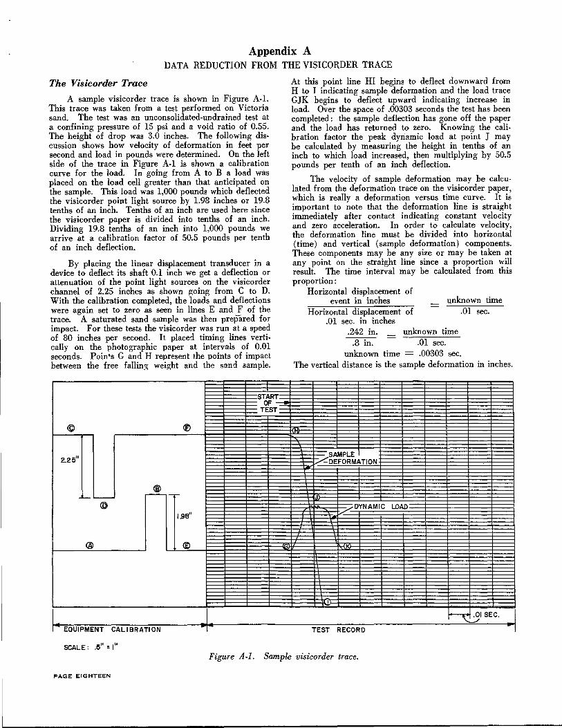
A sample visicorder trace is shown in Figure A-l. This trace was taken from a test performed on Victoria sand. The test was an unconsolidated-undrained test at a confining pressure of 15 psi and a void ratio of 0.55. The height of drop was 3.0 inches. The following discussion shows how velocity of deformation in feet per second and load in pounds were determined. On the left side of the trace in Figure A-1 is shown a calibration curve for the load. In going from A to B a load was placed on the load cell greater than that anticipated on the sample. This load was 1,000 pounds which deflected the visicorder point light source by 1.98 inches or 19.8 tenths of an inch. Tenths of an inch are used here since the visicorder paper is divided into tenths of an inch. Dividing 19.8 tenths of an inch into 1,000 pounds we arrive at a calibration factor of 50.5 pounds per tenth of an inch deflection.
By placing the linear displacement transducer in a device to deflect its shaft 0.1 inch we get a deflection or attenuation of the point light sources on the visicorder channel of 2.25 inches as shown ll:Oing from C to D. With the calibration completed, the loads and deflections were again set to zero as seen in lines E and F of the trace. A saturated sand sample was then prepared for impact. For these tests the visicorder was run at a speed of 80 inches per second. It placed timing lines vertically on the photographic paper at intervals of 0.01 seconds. Poin•s G and H represent the points of impact between the free fallin~ weight and the sand sample.
®
2.2511
~.-.-
1.9811
._ EQUIPMENT CALIBRATION
SCALE: .511 = 111
...
START OF
TEST
At this point line HI begins to deflect downward from H to I indicating sample deformation and the load trace GJK begins to deflect upward indicating increase in load. Over the space of .00303 seconds the test has been completed: the sample deflection has gone off the paper and the load has returned to zero. Knowing the calibration factor the peak dynamic load at point J may be calculated by measuring the height in tenths of an inch to which load increased, then multiplying by 50.5 pounds per tenth of an inch deflection.
The velocity of sample deformation may be calculated from the deformation trace on the visicorder paper, which is really a deformation versus time curve. It is important to note that the deformation line is straight immediately after contact indicating constant velocity and zero acceleration. In order to calculate velocity, the deformation line must be divided into horizontal (time) and vertical (sample deformation) components. These components may be any size or may be taken at any point on the straight line since a proportion will result. The time interval may be calculated from this proportion:
Horizontal displacement of event in inches unknown time
Horizontal displacement of .01 sec. in inches
.242 in. . 8 in.
unknown time .01 sec .
.01
unknown time = .00303 sec.
sec.
The vertical distance is the sample deformation in inches.
SAMPLE ~DEFORMATION
J /DYNAMIC LOAD
TEST RECORD
~:_91SEC . .. Figure A-1. Sample visicorder trace.
PAGE EIGHTEEN
To obtain this deformation the vertical component is measured and then divided by the attenuation:
Vertical length of Sample deformation = component in inches
2.25 inches of deflection .1 inch sample deformation
6.2 inches 2.25 inches
.1 inch
Sample deformation = .2755 inches
Velocity of deformation sample defoTmation
time length of event
.2755
.00303 = 91 ips
dividing by 12 to get velocity in feet per second,
Velocity of deformation = 7.6 fps.
Appendix B EXPLANATION OF COMPUTER PROGRAM
TO DETERMINE DAMPING CONSTANT
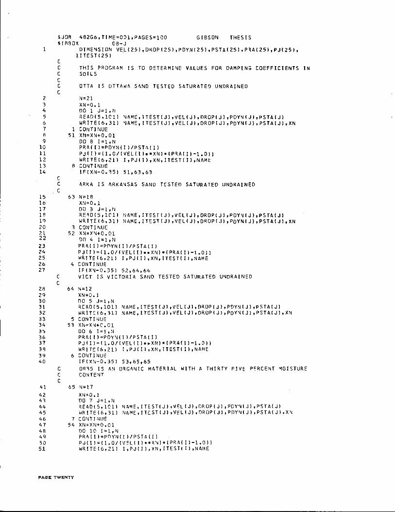
In modifying Smith's equation to determine a constant J, it was necessary to raise velocity of deformation to many different powers in order to arrive at an optimum power. To accomplish this, use was made of the IBM 360 Digital Computer. The program used to calculate the various J values is shown on pages 20-23. A flow diagram of this program is shown on page 24.
Use of the Computer Program
This program is made in sections, each section pertaining to a particular soil. For instance, in this investigation three sands were tested. Thus lines 2-14 (found on far left of program printout) represent Ottawa sand, 15-27 represent Arkansas sand and 28-40 represent Victoria sand. There must be one section for each soil or for each moisture content in the case of the cohesive materials. These sections are seen to be duplicates of one another with the following possible exceptions:
I. On lines 2, 15, 28, 41, 54, 67, 80, 93, 106, 119, 132, or the first card in each section is printed the number of data cards necessary for that particular soil. All data from one test will be put on one card.
2. The second card in each section indicates the lowest power to which velocity of deformation is to be raised. This should be a positive number to obey Smith's mathematical model.
3. In lines 8, 21, 34, 47, 60, 73, 86, 99, 112, 125, and 138 are seen the increments of the powers of velocity of deformation. In this case increments of 0.01 were used.
4. In lines 14, 27, 40, 53, 66, 79, 92, 105, 118, 131, and 144 are seen an "IF" statement which gives the highest power to which velocity may be raised. This
may be between the minimum described in step 2 and 1.0 which is Smith's power of velocity.
5. In lines 4, 7, 8, 9 and 13 for Ottawa sand are seen statement numbers. Statement numbers must not be duplicated if more sections are to be added to the program.
For this study the minimum power of velocity of deformation was 0.1 and the maximum was 0.36. Values of J were calculated for velocities of deformation in this range using an increment of 0.01.
One data card is required for each test performed. The information on each data card pertains to that particular test. Sample data are shown printed at the end of the program on page 77. The numbers in the following discussion which are referred to as decimal numbers should not exceed 10 digits total and should have no more than three digits to the right of the decimal point. The following input format is used for each data card:
I. In spaces 1-9 on the data card is printed any combination of numbers or letters describing the soil tested. This is a non-decimal number.
2. In spaces 10-19 on the data card is printed the number of the test which should be oriented to the right of the spaces allotted if it does not completely fill the space. This is a non-decimal number.
3. In spaces 20-29 on the card are printed velocity of deformation which is a decimal number.
4. In spaces 30-39 on the card is printed the height of drop which is a decimal number.
5. In spaces 40-49 on the card is printed the peak dynamic load in pounds which is a decimal number.
6. In spaces 50-59 on the card is printed the static load for the material which is a decimal number.
PAGE NINETEEN
$JOR 482G6,TIME=001,PAGES=l00 GIBSON THESIS $TRBQX 08-J
1 DIME~SION VELI25l,DKOP!25l,PDYNI25l,PSTAI25),P~A(25l,PJ{25l, liTESTI25l
c C THIS P~OGRAM IS TO DETERMI~E VALUES FOR DAMPIN~ COEFFICIENTS IN C SOl LS c C OTTA IS OTTAWA S~ND TESTED SATURATED UNDRAINED c
2 N=21 3 XN=0.1 4 DO 1 J=l,N 5 REA0(5,10ll ~AME,ITESTIJl,VEL!J),OROPIJl,PDY~IJ),pSTAIJl 6 WRITEI6,3ll ~AM~,ITESTIJ),VELIJ),OROPIJl,POYNIJ),PSTAIJ),XN
7 1 CONTINUE 8 51 XN=XN+0.01 9 DO 8 I =1, N
10 PRAIIl=PDYNIIl/PSTI\(Il 11 PJIIl=ll.O/IVELIIl**XNl*IPRAIIl-1.0)) 12 WRITEI6,2ll I,PJIIl,XN,ITESTIIl,NAME 13 8 CONTINUE 14 IFIXN-0.351 51,63,63
c C ARKA .IS 1\RKANSAS SAND TESTED SATURATED UNDRAINED c
15 63 N:;:l8 16 XN=0.1 17 DO 3 J=l.~ 1B RE~DI5,1C1l NAME,ITESTIJJ,VELIJ),OROPIJl,PDY~(J),pSTA(J) 19 WRITE(6,3ll NAME,ITESTIJJ,VELIJ),DROPIJ),PDYNIJl,PSTAIJl,XN 20 3 CONTINUC 21 52 XN=XN+0.01 22 on 4 I=1,N 23 PRI\IIl=PflYNIIl/PSTAIII 24 PJIIl=I1.0/(VELIII**XNI*IPRAIIl-l.Oll 25 WRITE16,2ll I,PJ!Il,XN,ITESTIIJ,NAME 26 4 CONTINUE 27 IF(XN-0.351 52,64,64
c c
28 29 30 31 32 33 34 35 36 37 38 39 40
c c c
41 42 41 44 lt5
46 47 48 49 50 51
VICT IS VICTORIA SAND TESTED SATURATED UNDRAINED
64 "l=l2 XN=O. 1 no 5 J=l,N ~CA0(5,10ll NAME,ITESTIJl,VELIJl,OROP(Jl,PDY~IJl,PSTAIJl WRITE(6,3ll NAME,ITESTIJl,VELIJ),OROPIJI,POYNIJJ,PSTA(J),XN
5 CONTihiU:: 53 XN=X·'J+O.C1
00 6 1=1 .~~ PRI\III=PDY'HII/PSTA(I) PJ(IJ=I1.0/IVELIIl**XNl*IPRAIIJ-1.0ll WRITE (6,21) I ,PJI I I ,XN, ITESTI I l ,NAME
6 CONTINUE IFIX\-0.351 53,6?,65 oq~5 IS AN ORGANIC M~TERIAL WITH A THIRTY FIV~ P~RCENT ~OISTURE CO\ITENT
65 N=l7 XN=O.l DO 7 J=l,N ~E~DI5,1C'll NAME,ITESTIJI,VELIJI,DROPIJI,PDY"JIJI,!•STAIJI WRITE(6,31l NAME,ITEST(J),VELIJ),DROPIJI,POYN(JI,PSTA(JI,X~
7 CONTINUE 54 XN=XN+O.Ol
DO 10 I=l,!\1 PRI\1 I I=Pf'lYNII l/PSTA( I I P J ( I I =I 1. 0 I IV !"Lt I I** X \l I* I PR .A I I I -1.0 I I WRITEI6,2ll I,PJ(li,XN,ITESTIII,NAr·1E
PAGE TWENTY
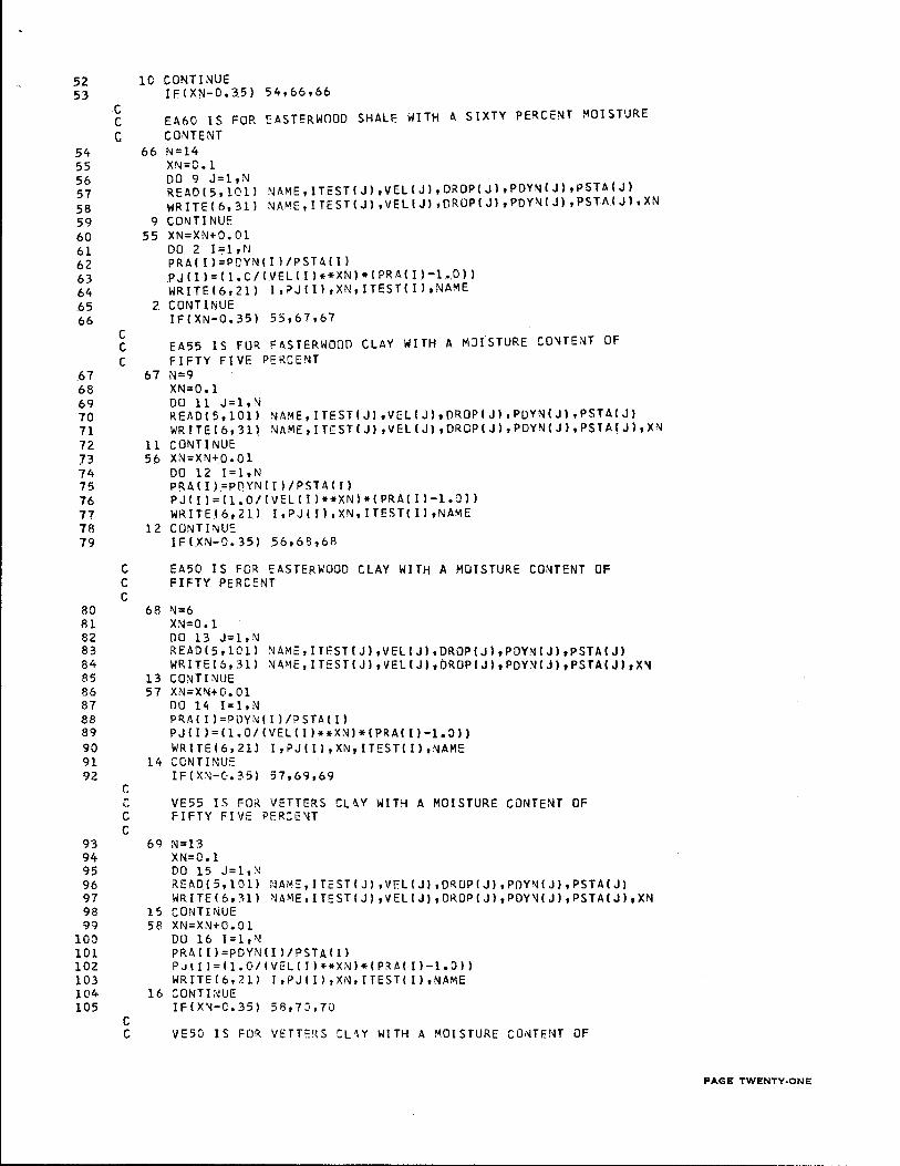
52 10 CONTINUE 53 IFIXN-0.~5) 54,66,66
g EA60 IS FOR [ASTERWOOD SHALF. WITH A SIXTY PERCE~T MOISTURE C CONTENT
54 66 N=l4 55 XN=C.l 56 DO 9 J=l,N 57 READ(5,10ll NAME,ITESTIJl,VEL(J),DROP(Jl,PDY~(J),pSTA(J} 58 WRITE(6,31l NAME,ITEST(JJ,VELIJ},OROP(J),PDY~(J),PST~IJ},XN 59 9 CONTINUE 60 55 XN=XN+0.01 61 DO 2 I~l,N 62 PRAIIl=PDYNIIl/PSTAIIl 63 PJIIl=ll.C/IVELIIl**XNl*IPRAIIJ-1~0}) 64 WRITEI6,2ll I,?JIIl 1 XN,ITESTIIl,NAME 65 2 CONTLNUE 66 IFIXN-0.351 55,67,67
c C EA55 IS FUR EASTERWOOD CLAY WITH A MJ(STURE CO~TENT OF C FIFTY FIVE PERCENT
67 67 N=9 68 XN=0.1 69 DO 11 J=l,N 70 READI5,101l NAME,ITEST(JJ,VELIJ),OROPIJl,POYNIJ),PSTAIJl 71 WRITE(6,31) NAME,ITESTIJ) 1 VELIJ),DROPIJl,PDYN(Jl,PSTAIJl,XN 72 11 CONTINUE 73 56 XN=XN+O.Q1 74 DO 12 I=l,N 75 PRAIIJ=PQYNI(l/PSTAIIl 7 6 P J I I ) = I 1. 0 I IV E L I I l **X N l *I PR A I I l -1. 0) l 77 WRITEI6,21l I,PJIIl,XN,ITEST(Il,NAME 78 12 CONTINU~ 7 9 IF I.X N- 0. 3 5 l 56, 6 '3, 6 8
C EA50 IS FOR EASTERWOOD CLAY WITH A MOISTURE CONTENT OF C FIFTY PERCENT c
80 68 N=6 81 XN=0.1 82 DO 13 J=l,N 83 READI5,1Cll NAME,ITESTIJl,VELIJl,DROP(Jl 1 PDYNIJl,PSTAIJl 84 WRITEl6,31l N~ME,ITESTIJ),VEL(J),OROPIJl,PDY~IJ),PSTAIJ),X~ 85 13 CONTINUE 86 57 XN=XN+O.Ol 87 DO 14 I=l,N 88 PRAIIl=POYN(Il/PSTAIIl 89 PJIIl=ll.O/IVELIIl**XN)*IPRA!Il-1.0}) 90 WRITEI6,21J I,PJIIl,XN,ITESTII),NAME 91 14 CONTINU~ 92 IFIXN-C'.35l 57,69,69
c C VE55 IS FOR VETTERS CL~Y WITH A MOISTURE CONTENT OF C FIFTY FIVE PER:E~T
c 93 69 N=13 94 XN=O.l 95 DO 15 J=l,~ 96 READI5,10ll NAM~,IT~STIJloVELIJl,OROPIJ),POY~IJ),PSTAIJ) 97 WRITE(6,31l ~AME,ITESTIJ),VELIJ),OROPIJl,PDY~IJl,PSTA(Jl,XN 98 15 CONTINUE 99 58 XN=XN+O.Ol
100 DO 16 I=l,~ 101 PRAIIl=PDYNIIl/PSTAIIl 102 PJ\Il=ll.O/IVELIIl**XNl*IPRAIIl-1.0)) 103 WRITEI6,21l I,PJII),XN,ITEST!Il,NAME 104 16 :ONTINUE 105 IFIX~-C.35l 58,7J,70
c C VE50 IS FOR VETT~RS CL\Y WITH A MOISTURE CONTENT OF
PAGE TWENTY-ONE

C FIFTY PERCENT c
106 70 :-.J=14 107 XN=0.1 108 DO 17 J=1.~ 109 ~EADI5 1 1Cll ~AME,IT~STI~l,VELtJI,DROPIJ),PDYNIJl,pSTAIJl 110 WRITE16,3ll ~A~E,ITESTIJl,VF.L!J),OROP(J),PDY~IJ),PSTAIJl,X~
111 17 CONTINUE 112 59 XN=XN+0.01 113 DO 18 I=1,~ 114 PRAIIl=f'fWNill/PSTAIIl 115 PJIIl=ll.O/IVELIIl••XNl•IP~AIIl-1.011 116 WRITEI6t.211 J,PJIIJ,XN,ITESTIIl,NAME 117 18 CONTINUE 118 IFIX~-0.351 5~,71,71
C VE46 IS FQq VETTERS :LAY WITH A MOISTURE CONT~~T OF C FORTY SIX DE~CE~T
119 71 ~=13 120 XN=0.1 121 DO 19 J = 1, ~ 122 READ15r10ll NI\~EtiT~STIJl ,VEL!J) 1 0KOPIJl,PDY'IJIJl 1 PSTAIJl 123 WRITEI6,31l ~AME,ITESTIJl 1 VEL!Jl,OROP!Jl,PDY~(Jl,PSTA!Jl,X~ 124 19 CO~TINU~ 125 60 XN=XN+C.~l 126 DO 2G 1=1.~ 127 PRA( I l=P[)Y"JI I l/PSTA( I l 128 P J I I l =I 1. 0 I( V :OL I I l ** Xr·!l *I PR A I I l-1. 0 l l 129 WRITEI6,?ll I,PJ(I),XN.ITESTIIJ,NAME 130 20 CONTI~UE 131 IFIX~-C.15l 60,72,72
C CE35 IS FU~ :E~TERVILLE SA~n WITH A ~DISTURE CJNTE~T OF C THIRTY FIV~ PE~C=NT
c 132 72 ~=13
133 XN=O.l 134 DO 23 J=1,N 135 READ!5 1 101l 'IJAME,ITESTIJl,VEL(J),DROP!Jl,PDYN!Jl,PSTAIJl 136 WRITE!6,31l NAME,ITEST!Jl,VEL!Jl,DROP(JlrPDYN!JlrPSTA!JlrXN 137 23 CONTINUE 138 61 XN=XN+0.01 139 DO 22 I=l 1 N 140 PRA!ll=PnYN!!)/PSTAJil 141 PJ! I 1=1 1.0/!VEL! I Jux;•JI•IPRA( I l-1.0)) 142 WRITE!6r2ll I ,pJ(I l ,XN,ITEST!Il ,NAME 143 22 CONTINUE 14.4 IFIXN-0.35) 6lr73,73 145 21 FORMAT!10X,I4,10X,F10.3,10X,F10.3r10X,I4r'10X,A4) 146 31 FDRMATIA4,5X,I3,6X,FB.5r2X,F8.5,3X,F7.3r3X,F~.3,3X,F6.4) 14 7 1 0 1 F 0 R M AT I A 4 , 5 X , I 3 , 6 X , F 8 • 5 , 2 X , F 8 • 5 , 3 X , F 7 • '3 , 3 X , F 7 • 3 ) 148 73 CONTINUE 149 102 STOP 150 ENfl
SAMPLE DATA
TEST VELOCITY OF HEIGHT DYNAMIC STATIC MATERIAL NO. DEFORMATION OF DROP LOAD LOAD
EA50 115 0. 99700 o.ooooo 125.000 63.500 EA50 l14 2. 900C'·O l.:J::lOOO 134.500 63.500 EA50 113 4.40000 2.00000 136.400 63.500 EA50 112 5.48000 3.0::l000 144.000 63.500 EA50 111 9.04000 9.0:)000 154.500 63.500 EA50 110 10.31999 12.0::>000 156.000 63.500
PAGE TWENTY·TWO

ITERATION TEST NUMBER J-VALUE N NO. MATERIAL
6 l.D51 0.140 110 EA50 1 0.969 0.150 115 EA50 2 0.95~ 0.150 114 EA50 3 o. 919 0.150 113 EA50 4 o. '}82 0.150 112 EA50 5 1. :)30 0.150 111 EASO 6 1.026 0.150 110 EA50 1 C.969 0.160 115 EA50 2 0.943 0.160 114 EA50 3 0.106 0.160 113 EA5'0 4 0. '~ 66 0.160 112 EA50 5 l.OOB 0.160 111 EA50 6 1. 0:)3 0.160 11:> EA50 1 0.969 0.1n 115 EA50 2 0.933 0.170 114 EA50 3 o. '392 0.170 113 EA50 4 0.949 0.170 112 EA50 5 0.986 0.170 111 EA50 6 0.9fl0 0.170 110 EA50 1 0.969 o .tao 115 EASO 2 0.923 0.180 114 EA50 3 0.879 0.180 113 EA50 4 0.933 0.180 112 EA50 5 0.964 0. 180 111 Ell SO 6 0.957 0.180 lD EA50 1 0.969 0.190 115 EA50 2 0.913 0.190 114 EA50 3 0.866 0.190 113 EA50 4 ').91R 0.190 112 EA50 5 0.943 0.190 111 EA50 6 0.93'> 0.190 110 EA50
PAGE TWENTY-THREE
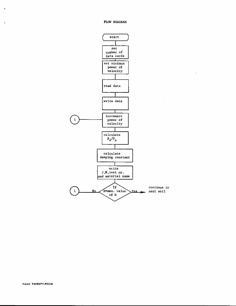
No
PAGE TWENTY-FOUR
FLOW DIAGRAM
set number of data .cards
set minimum power of velocity
read data
write data
increment power of velocity
calculate damping constant
write J,N,test no.
and material name
continue to next soil
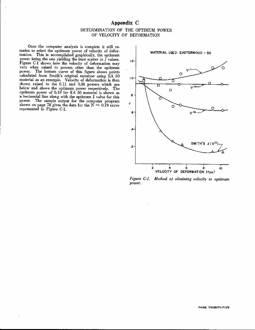
Appendix G DETERMINATION OF THE OPTIMUM POWER
OF VELOCITY OF DEFORMATION
Once the computer analysis is complete it still remains to select the optimum power of velocity of deformation. This is accomplished graphically, the optimum power being the one yielding the least scatter in J values. Figure C-1 shows how the velocity o·f deformation may vary when raised to powers other than the optimum power. The bottom curve of this figure shows points calculated from Smith's original equation using EA 50 material as an example. Velocity of deformation is then shown raised to the 0.11 and 0.36 powers which are below and above the optimum power respectively. The optimum power of 0.19 for EA 50 material is shown as a horizontal line along with the optimum J value for this power. The sample output for the computer program shown on page 78 gives the data for the N = 0.19 curve represented in Figure C-1.
MATERIAL USED: EASTERWOOD- 50
1.2
y.ll
1.0
.8
J
.6
SMITH'S J ( yi.0 l .2
2 4 6 8 10 VELOCITY OF DEFORMATION (fps)
Figure C-1. Method of obtaining velocity to optimum power.
PAGE TWENTY-FIVE
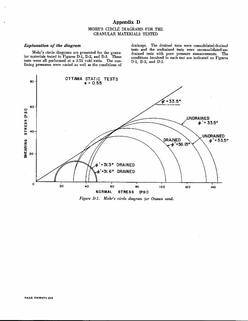
Appendix D MOHR'S CIRCLE DIAGRAMS FOR THE
GRANULAR MATERIALS TESTED
Explanation of the diagram drainage. The drained tests were consolidated-drained tests and the undrained tests were unconsolidated-undrained tests with pore pressure measurements. The conditions involved in each test are indicated on Figures D-1, D-2, and D-3.
Mohr's circle diagrams are presented for the granular materials tested in Figures D-1, D-2, and D-3. These tests were all performed at a 0.55 void ratio. The confining pressures were varied as well as the conditions of
80
60 -U)
~ ~ U)
laJ a:: 1- 40 U)
(!)
z a:: <t laJ 20 J: U)
0 20
OTTAWA STATIC TESTS e = 0.55
40
DRAINED
DRAINED
60 80
NORMAL STRESS (PSI) 100
Figure D-1. Mohr's circle diagram for Ottawa sand.
PAGE TWENTY-SIX
UNDRAINED 4> I: 33.5°
12.0 140
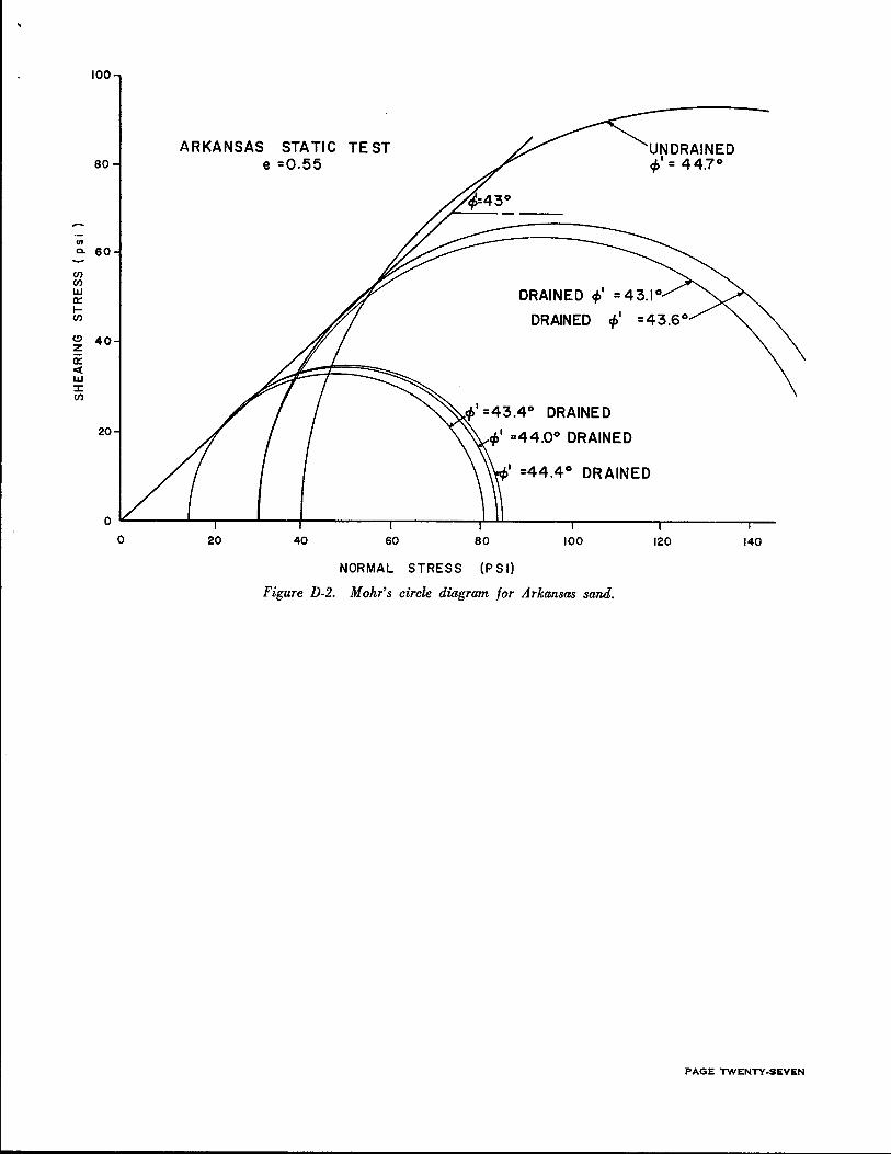
·-VI a.
en en UJ a: 1-en
(!)
z ii: <( UJ :::z:: en
100
80
60
40
20
ARKANSAS STATIC TEST e =0.55
UNDRAINED cp1
= 44.7°
DRAINED cp' = 43.1°
DRAINED
"'' =43.4° DRAINED
cp1 =44.0° DRAINED
I =44.4° DRAINED
0 ~----~~----L---+-------~--------~~------~-------r--------r--0 20 40 60 80 100 120 140
NORMAL STRESS (PSI)
Figure D-2. Mohr's circle diagram for Arkansas sand.
PAGE TWENTY-SEVEN
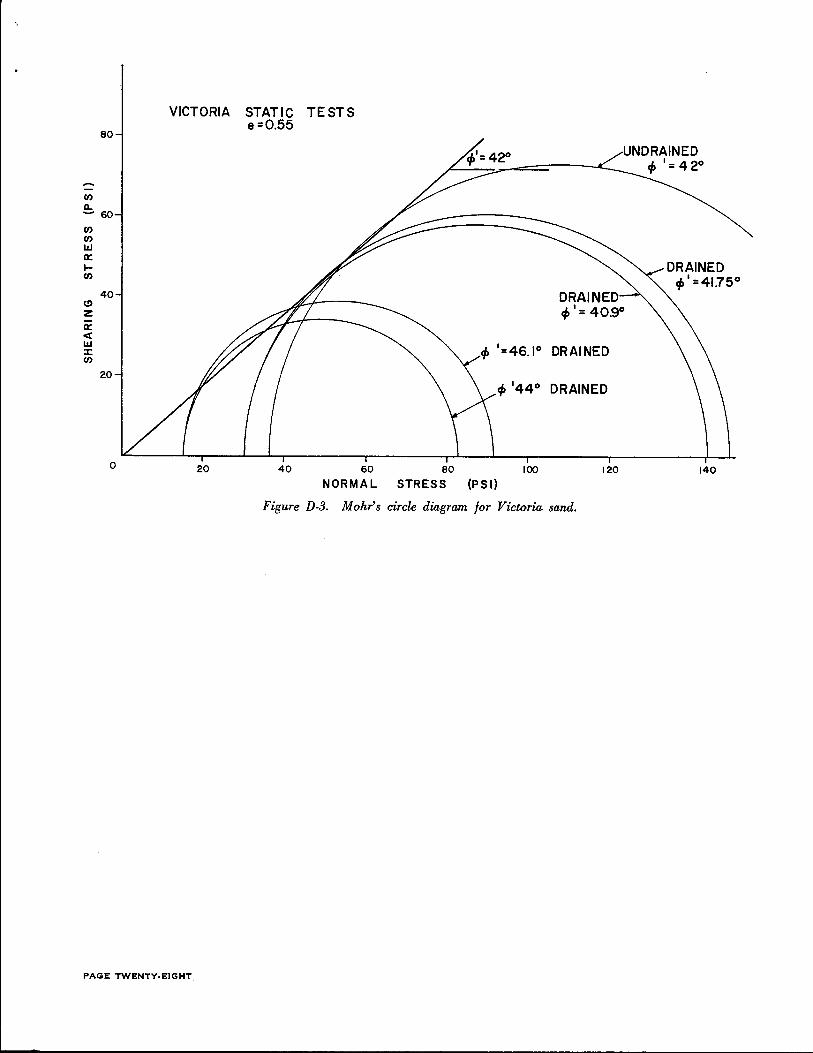
C/)
0..
80
~ 60
C/) C/)
LLI 0:: ..... C/)
(!)
z 0:: <( LLI ::1: C/)
40
20
0
VICTORIA STATIC TESTS e=0.55
20 40 60 80
NORMAL STRESS (PSI)
DRAINED
<j1 '44° DRAINED
100 120
Figure D-3. Mohr's circle diagram for Victoria sand.
PAGE TWENTY-EIGHT
140


![Soil-structure interaction analysis of RC frame shear wall ......Soil-structure interaction analysis of RC frame . ... damping of 5% [7] considering fixed base condition and a. lso](https://cdn.vdocuments.us/doc/165x107/5e3f329522fc1874f61be1c1/soil-structure-interaction-analysis-of-rc-frame-shear-wall-soil-structure.jpg)


