
AQR Capital Management, LLC
Two Greenwich Plaza
Greenwich, CT 06830
p: +1.203.742.3600 | w: aqr.com
Smarter Saving and Investing in a Lower Expected Return World
Principal
Antti Ilmanen, Ph.D.
Prepared for the PRC conference
Philadelphia, May 4-5, 2017

Disclosures
The information set forth herein has been obtained or derived from sources believed by AQR Capital Management, LLC (“AQR”) to be reliable. However, AQR does not make any
representation or warranty, express or implied, as to the information’s accuracy or completeness, nor does AQR recommend that the attached information serve as the basis of
any investment decision. This document has been provided to you solely for information purposes and does not constitute an of fer or solicitation of an offer, or any advice or
recommendation, to purchase any securities or other financial instruments, and may not be construed as such. This document is intended exclusively for the use of the person to
whom it has been delivered by AQR and it is not to be reproduced or redistributed to any other person. Please refer to the Appendix for more information on risks and fees. Past
performance is not a guarantee of future performance.
This presentation is not research and should not be treated as research. This presentation does not represent valuation judgments with respect to any financial instrument, issuer, security or sector that may be described or referenced herein and does not represent a formal or official view of AQR.
The views expressed reflect the current views as of the date hereof and neither the speaker nor AQR undertakes to advise you of any changes in the views expressed herein. It should not be assumed that the speaker will make investment recommendations in the future that are consistent with the views expressed herein, or use any or all of the techniques or methods of analysis described herein in managing client accounts. AQR and its affiliates may have positions (lo ng or short) or engage in securities transactions that are not consistent with the information and views expressed in this presentation.
The information contained herein is only as current as of the date indicated, and may be superseded by subsequent market events or for other reasons. Charts and graphs provided herein are for illustrative purposes only. The information in this presentation has been developed internally and/or obtained from sources believed to be reliable; however, neither AQR nor the speaker guarantees the accuracy, adequacy or completeness of such information. Nothing contained herein c onstitutes investment, legal, tax or other advice nor is it to be relied on in making an investment or other decision.
There can be no assurance that an investment strategy will be successful. Historic market trends are not reliable indicators of actual future market behavior or future performance of any particular investment which may differ materially, and should not be relied upon as such. Target allocations contained herein are subject to change. There is no assurance that the target allocations will be achieved, and actual allocations may be significantly different than that shown here. Thi s presentation should not be viewed as a current or past recommendation or a solicitation of an offer to buy or sell any securities or to adopt any investment strategy.
The information in this presentation may contain projections or other forward‐looking statements regarding future events, targets, forecasts or expectations regarding the
strategies described herein, and is only current as of the date indicated. There is no assurance that such events or targets will be achieved, and may be significantly different from that shown here. The information in this presentation, including statements concerning financial market trends, is based on c urrent market conditions, which will fluctuate and may be superseded by subsequent market events or for other reasons. Performance of all cited indices is calculated on a total return basis with dividends reinvested.
The investment strategy and themes discussed herein may be unsuitable for investors depending on their specific investment ob jectives and financial situation. Please note that changes in the rate of exchange of a currency may affect the value, price or income of an investment adversely.
Neither AQR nor the speaker assumes any duty to, nor undertakes to update forward looking statements. No representation or wa rranty, express or implied, is made or given by or on behalf of AQR, the speaker or any other person as to the accuracy and completeness or fairness of the information contained in this presentation, and no responsibility or liability is accepted for any such information. By accepting this presentation in its entirety, the recipient acknowledges it s understanding and acceptance of the foregoing statement.
2

The Low Expected Return Challenge

4
Sources: AQR, Robert Shiller’s web site, Kozicki-Tinsley (2006), Federal Reserve Bank of Philadelphia, Blue Chip Economic Indicators, Consensus Economics, Morningstar. Prior to 1926, stocks are represented by a reconstruction of the S&P 500 available on Robert Shiller’s web site which uses dividends and earnings data from Cowles and associates, interpolated from annual data. After that, stocks are the S&P 500. Bonds are represented by long-dated Treasuries. The 60/40 Expected Real Yield is represented by Stocks/Bonds. The equity yield is a 50/50 mix of two measures: 50% Shiller E/P * 1.075 and 50% Dividend/Price + 1.5%. Scalars are used to account for long term real Earnings Per Share (EPS) Growth. Bond yield is 10 year real Treasury Yield over 10 year inflation forecast as in Expected Returns (Ilmanen, 2011), with no rolldown added. Chart is for illustrative purposes only. Past performance is not a guarantee of future performance. Please read important disclosures in the Appendix.
Expected Real Return of the U.S. 60/40 Stock/Bond Portfolio January 1900–December 2016
A World of Lower Expected Returns Expected Returns for Long-Only Assets Are Lower Than in the Past
Expected returns for 60/40 averaged 5% real in 1900s, fell to 2-2.5% in recent years. Not just bonds but also stocks have starting yields low compared to history.
Can apply to all long-only investments when the common part of discount rates is near all-time lows
These yield-based estimates are of little use for tactical market timing but :they give a useful anchor for next 5-10-year returns, and maybe beyond
0%
2%
4%
6%
8%
10%
12%
14%
1900 1910 1920 1930 1940 1950 1960 1970 1980 1990 2000 2010
U.S. 60/40 Real Yield
Long-term Average
2.3%

Maybe The Generational Problem for the Coming Decades
5
We Try to Quantify the Challenge and Offer Solutions for Various Investor Types

How Much Should DC Savers Worry About Expected Returns?

Overview
7
How Much Should DC Savers Worry About Expected Returns?
Source: AQR. Past performance is not a guarantee of future performance.
Many plan sponsors assume that long-term returns will be similar to those of the past few decades
Unfortunately, current market yields indicate that both stocks and bonds may deliver lower returns
This may mean that participants need to significantly increase their savings rates to reach a given retirement target income
We believe that for participants to achieve their retirement goals, plan sponsors should focus on: incentivizing saving and identifying investments that have the potential to enhance returns (with reasonable risk).
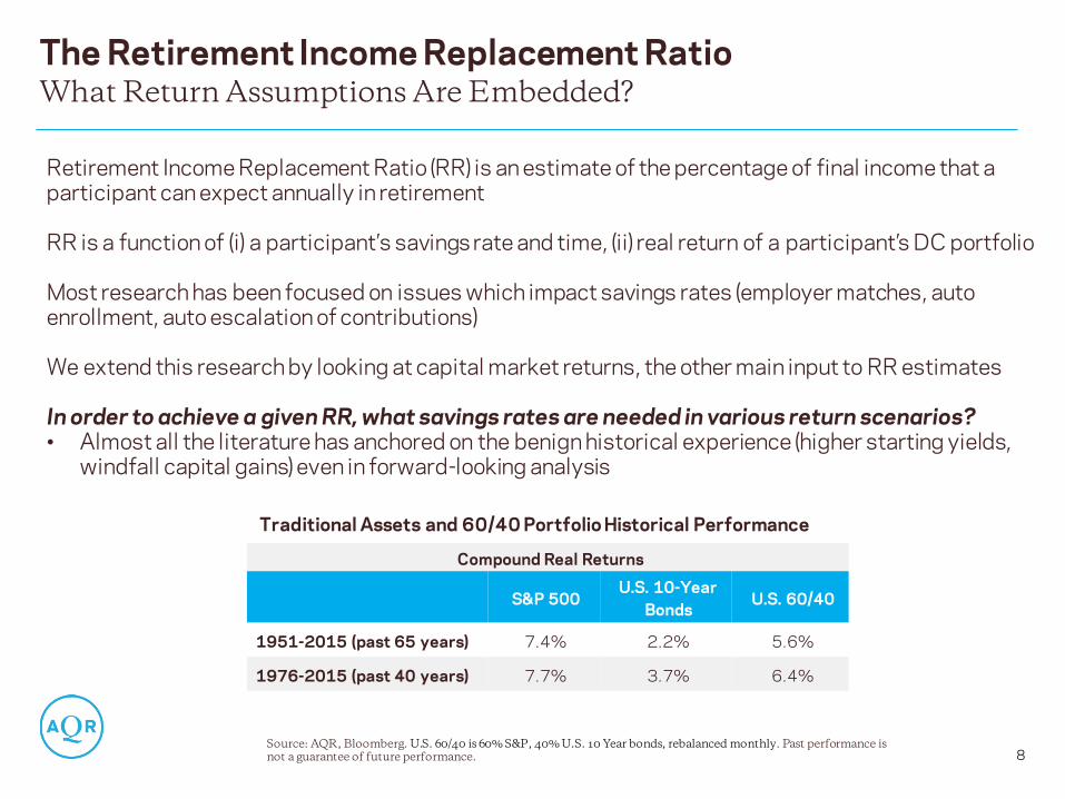
The Retirement Income Replacement Ratio
8
What Return Assumptions Are Embedded?
Source: AQR, Bloomberg. U.S. 60/40 is 60% S&P, 40% U.S. 10 Year bonds, rebalanced monthly. Past performance is not a guarantee of future performance.
Retirement Income Replacement Ratio (RR) is an estimate of the percentage of final income that a participant can expect annually in retirement
RR is a function of (i) a participant’s savings rate and time, (ii) real return of a participant’s DC portfolio Most research has been focused on issues which impact savings rates (employer matches, auto enrollment, auto escalation of contributions)
We extend this research by looking at capital market returns, the other main input to RR estimates In order to achieve a given RR, what savings rates are needed in various return scenarios? • Almost all the literature has anchored on the benign historical experience (higher starting yields,
windfall capital gains) even in forward-looking analysis
Compound Real Returns
S&P 500 U.S. 10-Year
Bonds U.S. 60/40
1951-2015 (past 65 years) 7.4% 2.2% 5.6%
1976-2015 (past 40 years) 7.7% 3.7% 6.4%
Traditional Assets and 60/40 Portfolio Historical Performance

Base Case
9
If Historical Returns Are Repeated, 8% Savings Rate May Be Enough
We first assume that the DC saver holds the U.S. 60/40 portfolio, which delivers the historical real return of approximately 5.5% p.a. Other assumptions:
• 2% p.a. real income growth over a 40-year saving period
• 25-year annuity purchased at retirement (the income from which is used to compute RR)
• Target total RR of 75%, where 30% is assumed to come from sources outside the plan, and 45% comes from DC savings
Based on these assumptions, an 8% annual savings rate is required to achieve a 75% RR
Source: Morningstar, GFD, Datastream, AQR. S&P 500 is the SBBI series “U.S. Large Stock TR USD.” U.S. 10 Year bonds provided by GFD prior to 1980 and Datastream thereafter. U.S. 60/40 is 60% S&P, 40% U.S. 10 Year bonds, rebalanced monthly. Historical return calculated over period 1951-2015. Returns are excess of CPI. Time periods are chosen to represent a savings and retirement period (~65 years) and just a savings period (~40 years). Assumptions are discussed in Ilmanen, Rauseo and Truax (2016) Appendix A. 2% real income growth reflects both productivity growth and career progression. 75% target RR balances likely lower cost of housing, need for saving, and spending dependents versus the potentially higher cost of health care. Hypothetical data has inherent limitations, some of which are disclosed in the Appendix hereto. Please read important disclosures in the Appendix.

6%
8%
11%
15%
19%
0%
5%
10%
15%
20%
25%
6.5% 5.5%
Historical Return
4.5% 3.5%
Realistic Assumption
2.5%
Sa
vin
gs
Ra
te
U.S. 60/40 annual real return expectation
The Trade-Off Between Returns and Savings Rates
10
Lower Expected Returns = Higher Required Savings
* See AQR Alternative Thinking Q1 2017: Capital Market Assumptions for Major Asset Classes. Real return assumptions of 5% for equities and 1% for bonds reflect low current real yields but also assume some normalization over the saving period.
Source: AQR, calculated using the assumptions laid out on this and the previous slide. U.S. 60/40 Annual Return Expectations reflect a portfolio invested 60% in U.S. equities and 40% in U.S. bonds. U.S. equities and U.S. bonds are based on simulations using the returns stated in this section. U.S. equities is meant to be representation of a large capitalization broad U.S. equity index like the S&P 500 index; U.S. bonds is meant to be representative of a broad bond index like the Barclays U.S. Aggregate. Historical return is based on period 1951-2015. We only show savings rates in full percentage points to avoid false precision of our estimates. For illustrative purposes only. Hypothetical data has inherent limitations, some of which are disclosed in the Appendix hereto. Please read important disclosures in the Appendix
Below we show required savings rates for a range of different return assumptions
Lower real return assumptions anchored to current real yields* imply a 15% required savings rate, compared to 8% savings rate using historical returns
• We assume 5% for stocks, 1% for bonds; ca. 3.5% for 60/40 (still above next-decade outlook)
• Each 1% decrease in expected returns leads to a 2-5% increase in required savings rate
• In order to compensate for lower returns, participants may have to save meaningfully more
Impact of Lower Return Expectations on Savings Rate Required to Achieve 75% RR
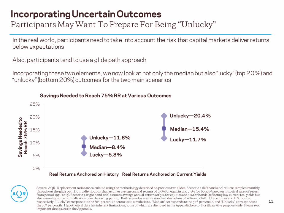
Incorporating Uncertain Outcomes
11
Participants May Want To Prepare For Being “Unlucky”
Source: AQR. Replacement ratios are calculated using the methodology described on previous two slides. Scenario 1 (left hand side) returns sampled monthly throughout the glide path from a distribution that assumes average annual returns of 7.5% for equities and 2.5% for bonds (based on historical rates of return from period 1951-2015). Scenario 2 (right hand side) assumes average annual returns of 5% for equities and 1% for bonds (reflecting low current real yields but also assuming some normalization over the saving period). Both scenarios assume standard deviations of 15% and 5% for U.S. equities and U.S. bonds, respectively. “Lucky” corresponds to the 80th percentile across 1000 simulations, “Median” corresponds to the 50th percentile, and “Unlucky” corresponds to the 20th percentile. Hypothetical data has inherent limitations, some of which are disclosed in the Appendix hereto. For illustrative purposes only. Please read important disclosures in the Appendix.
In the real world, participants need to take into account the risk that capital markets deliver returns below expectations Also, participants tend to use a glide path approach Incorporating these two elements, we now look at not only the median but also “lucky” (top 20%) and “unlucky” (bottom 20%) outcomes for the two main scenarios
0%
5%
10%
15%
20%
25%
Real Returns Anchored on History(Scenario 2)
Real Returns Anchored on Current Yields(Scenario 4)
Sa
vin
gs
Ne
ed
ed
to
R
ea
ch
75
% R
R
Median—8.4%
Unlucky—11.6%
Lucky—5.8%
Median—15.4%
Unlucky—20.4%
Lucky—11.7%
Savings Needed to Reach 75% RR at Various Outcomes

Better Investing: The Big Picture

13
2. Add Illiquids Illiquidity; contain much equity beta; also historically expensive
Endowment Model Beliefs: High returns historically; perceived illiquidity premium
1. More Equities Concentration: already dominant risk to many; not cheap
CAPM Beliefs: Highest conviction potential long-term return source
3. Add Factor Tilts and Alternative Risk Premia
Leverage and other tools are required to meet return targets
Multi-Factor Beliefs: Evidence on multiple rewarded factors, potential diversification benefits
Possible Solution Motivation
Source: AQR. Diversification does not eliminate the risk of experiencing investment losses. Past performance is not a guarantee of future performance
What Can Investors Do? Three Broad Paths to Address the Low Expected Return Challenge
Challenges

What Can Investors Do?
14
Three Broad Paths to 5% Expected Real Return, Even Today
Source: AQR. For illustrative purposes only and not representative of an actual portfolio AQR manages. Allocation analysis is based on expected real return, volatility, correlation and leverage assumptions shown in the Appendix. For further details and discussion on long-term expected return estimates, see AQR Alternative Thinking Q1 2017: Capital Market Assumptions for Major Asset Classes. For volatility and correlation assumptions: Global Equity (cap-weighted and factor-tilted) is based on the MSCI World Index; Global Fixed Income (cap-weighted and factor-tilted) is based on the Barclays Global Aggregate Index (hedged); Private Equity is based on the Cambridge Associates LLC U.S. Private Equity Index, with returns adjusted to account for smoothing; Alternative Risk Premia is based on a hypothetical multi-asset long/short style strategy as described in the appendix. There is no guarantee, express or implied, that long-term return and/or volatility targets will be achieved. Realized returns and/or volatility may come in higher or lower than expected. Hypothetical performance results have certain inherent limitations, some of which are disclosed in the Appendix. Please read important disclosures in the Appendix.
Investment 60/40
(cap-wtd) 1. Go to Equities 2. Add Illiquids
3. Add Factor Tilts and ARP
Global Equity (cap-weighted) 60% 67% 60% 0%
Global FI (cap-weighted) 40% 0% 11% 0%
Private Equity 0% 0% 29% 0%
Global Equity (factor-tilted) 0% 33% 0% 60%
Global FI (factor-tilted) 0% 0% 0% 29%
Alternative Risk Premia 0% 0% 0% 11%
Investment 60/40
(cap-wtd) 1. Go to Equities 2. Add Illiquids
3. Add Factor Tilts and ARP
Leverage (look-through) No No Yes Yes
Expected Volatility 9% 15% 13% 9%
Expected Real Return 3% 5% 5% 5%

Long-Term Capital Market Assumptions
15
Ex Ante Assumptions for Investments in “5% Real” Recipes
* For further details and discussion on long-term expected real return assumptions, see AQR Alternative Thinking Q1 2017: Capital Market Assumptions for Major Asset Classes.
Source: AQR. For volatility and correlation assumptions: Global Equity (cap-weighted and factor-tilted) is based on the MSCI World Index; Global Fixed Income (cap-weighted and factor-tilted) is based on the Barclays Global Aggregate Index (hedged); Private Equity is based on the Cambridge Associates LLC U.S. Private Equity Index, with returns adjusted to account for smoothing; Alternative Risk Premia is based on a hypothetical multi-asset long/short style strategy as described in the appendix. There is no guarantee, express or implied, that long-term return and/or volatility targets will be achieved. Realized returns and/or volatility may come in higher or lower than expected. Hypothetical performance results have certain inherent limitations, some of which are disclosed in the Appendix. Please read important disclosures in the Appendix.
Expected Real Return assumptions are based on yield-based
estimates for equities and bonds; assumed illiquidity premium
for private equity; and for alternative risk premia and factor tilts
a combo of discounted hypothetical performance and judgment
For cash, the assumption of 0% real return reflects the current
low-yield environment with some expectation of normalization
Volatilities and correlations based on hypothetical and proxy index performance, rounded
Correlations
Investment Expected
Real Return
Volatility
Global Equity (cap-weighted) 4.5% 15.0%
Global FI (cap-weighted) 1.0% 5.0%
Private Equity 7.5% 15.0%
Global Equity (factor-tilted) 6.0% 15.0%
Global FI (factor-tilted) 2.0% 5.0%
Alternative Risk Premia 7.5% 10.0%
Cash 0.0%
Investment Global Equity
(cap-wtd) Global FI (cap-wtd)
Private Equity
Global Equity (factor tilted )
Global FI (factor tilted )
Alternative Risk Premia
Global Equity (cap-weighted) 1.0 0.0 0.9 1.0 0.0 0.0
Global FI (cap-weighted) 0.0 1.0 0.0 0.0 1.0 0.0
Private Equity 0.9 0.0 1.0 0.9 0.0 0.0
Global Equity (factor-tilted) 1.0 0.0 0.9 1.0 0.0 0.0
Global FI (factor-tilted) 0.0 1.0 0.0 0.0 1.0 0.0
Alternative Risk Premia 0.0 0.0 0.0 0.0 0.0 1.0

Example of ‘Better Investing’ Given Multi-Factor Beliefs: Balancing on the Life-Cycle – Improving Under-diversified TDFs*
* This example is not directly tied to the previous section because we use risk parity rather than alternative risk premia as the main way to improve risk diversification

How Traditional Target Date Funds (TDFs) Might Be Improved
17
Diversification, Diversification, Diversification
Source: AQR. This list may not be comprehensive. Diversification does not eliminate the risk of experiencing investment losses.
Shortcoming / Source of Under-Diversification
Proposed Solution / Source of Better Diversification
1. Home-Biased Investing Invest Globally
2. Few Inflation-Protection Assets Add Commodities (etc.)
3. Equity Risk Concentration Risk Balanced Allocations
4. Sensitivity To Volatile Periods Dynamic Risk Targeting
5. Lack of Diversifying Alternatives Incorporate Trend-Following (etc.)

Empirical Benefits of Better Diversification (Full Shift)
18
Addressing Each of These Shortcomings Has Improved Hypothetical Results
Source: AQR. For illustrative purposes only and not based on an actual portfolio AQR manages. Please see slide 28 for an explanation of the methodology used and slide 31 for detail on the underlying dataset. Hypothetical analysis is gross of fees and t costs. Traditional U.S. is domestic 80% U.S. equities/20% U.S. fixed income. Traditional Global is 80% global equities/20% global fixed income. Traditional Global + 10% Commodities is 72% global equities/18% global fixed income/10% commodities. Global equities and global fixed income are GDP-weighted across available countries. Commodities is an equal-weighted portfolio of available commodities. Risk Parity without Vol Targeting is a simple equal risk portfolio of global equities, global fixed income, and commodities. Risk Parity with Vol Targeting is a simple equal risk portfolio of global equities, global fixed income, and commodities that targets a constant annual volatility. Risk Parity + 10% trend is 90% Risk Parity with Vol targeting and 10% Trend-Following. Hypothetical data has inherent limitations, some of which are disclosed in the appendix hereto. Please read important disclosures in the Appendix.
0.38
0.51 0.54
0.61 0.64
0.76
0
0.2
0.4
0.6
0.8
Traditional U.S. Traditional Global Traditional Global+ 10%
Commodities
Risk Parity withoutVol Targeting
Risk Parity with VolTargeting
Risk Parity+ 10% Trend
Sh
arp
e R
ati
o (n
et
of
t-c
os
ts)
Stepwise Sharpe Ratio Improvement of Hypothetical Simple Portfolio, 1903–2014

Adding as a Component to Traditional TDFs (Partial Shift)
19
Each Solution May Add Value, a Combination May Be Even Better
Source: AQR. For illustrative purposes only and not based on an actual portfolio AQR manages. Please see slide 28 for an explanation of the methodology used and slide 31 for detail on the underlying dataset. TDF strategies are gross of fees and t-costs and use the average glide path across the three largest TDF providers as of June 2014. Hypothetical risk parity and trend strategies are gross of fees and net of t costs. Please see footnote on the previous slide for an explanation of the composition of each portfolio shown. Hypothetical data has inherent limitations, some of which are disclosed in the appendix hereto. 10% Best and 10% Worst are averages. “Average Risk” is the average volatility each cohort faced over its savings period. Please read important disclosures in the Appendix.
8%
9%
10%
11%
12%
13%
$100,000
$200,000
$300,000
$400,000
$500,000
TraditionalU.S.
TraditionalGlobal
TraditionalGlobal + 10%Commodities
Risk Paritywithout VolTargeting
Risk Paritywith Vol
Targeting
Risk Parity +10% Trend
Av
era
ge
Ris
k (
Vo
lati
lity
)
Re
tire
me
nt
We
alt
h (
Re
al)
10% Best
Average
10% Worst
Average Risk
1 Idea #: 2 3 4 5

Conclusion of the TDF Analysis
20
Better Diversification May Also Help Returns
Source: AQR. Hypothetical data has inherent limitations, some of which are disclosed in the appendix hereto. Diversification does not eliminate the risk of experiencing investment losses.
We believe these ideas address lifetime investing goals through:
• A more-explicit focus on risk management
• Less importantly, inclusion of return-enhancing strategies
• Benefiting from better risk balance across asset classes and strategies
• Addressing tail risk, particularly in the last decade before retirement
Thoughts for implementation:
• These solutions are “alternative” (unconventional; efficient diversification would require manager use of shorting and leverage)
• However, few are “new” to the investment scene, many have 10+ year institutional track records, are supported by academic research, and are increasingly used by institutional investors
• Likelihood of success may be better as a diversifying “sleeves” within a TDF: Evolution rather than revolution is more realistic, given common constraints.

Appendices - Expected Real Return History on Stocks and Bonds - Other Long-Run Return Sources - Some Empirical Evidence - Real-World Constraints - Details on the TDF Analysis

-2%
0%
2%
4%
6%
8%
10%
12%
1900 1910 1920 1930 1940 1950 1960 1970 1980 1990 2000 2010
U.S. 60/40 Expected Real Return U.S. 60/40 Realized Next 20Y Real Return Historical Average
22
Sources: AQR, Robert Shiller’s web site, Kozicki-Tinsley (2006), Federal Reserve Bank of Philadelphia, Blue Chip Economic Indicators, Consensus Economics, Morningstar. Prior to 1926, stocks are represented by a reconstruction of the S&P 500 available on Robert Shiller’s web site which uses dividends and earnings data from Cowles and associates, interpolated from annual data. After that, stocks are the S&P 500. Bonds are represented by long-dated Treasuries. The 60/40 Expected Real Yield is represented by Stocks/Bonds. The equity yield is a 50/50 mix of two measures: 50% Shiller E/P * 1.075 and 50% Dividend/Price + 1.5%. Scalars are used to account for long term real Earnings Per Share (EPS) Growth. Bond yield is 10 year real Treasury Yield over 10 year inflation forecast as in Expected Returns (Ilmanen, 2011), with no rolldown added. Chart is for illustrative purposes only. Past performance is not a guarantee of future performance. Please read important disclosures in the Appendix.
Expected Real Return of U.S. Stocks, Bonds and the 60/40 Portfolio January 1900–December 2016
2.3%
3.8%
0.2%
Challenge: A World of Low Expected Returns
Prospective Real Returns Are Low For Both Stocks and Bonds
-5%
0%
5%
10%
15%
20%
1900 1910 1920 1930 1940 1950 1960 1970 1980 1990 2000 2010
U.S. Equity Real Yield U.S. 10Y Treasury Real Yield
5.0%

Multiple Rewarded Factors
23
Well-Known, Global Return Premia as Long-Run Sources of Return
Source: AQR. Diversification does not eliminate the risk of experiencing investment losses. Past performance is not a guarantee of future performance.
Momentum The tendency for an asset’s recent relative performance to continue in the near future
Value The tendency for relatively cheap assets to outperform relatively expensive ones
Carry The tendency for higher-yielding assets to provide higher returns than lower-yielding assets
Defensive The tendency for lower risk and higher-quality assets to generate higher risk-adjusted returns
Illiquidity The tendency for illiquid assets (e.g., PE, small-caps stocks) to outperform more liquid ones
Bonds Returns from bearing interest rate risk
Equities Returns from the equity risk premium
Inflation Returns from inflation-sensitive assets
Market Risk Premia
Relative-Value Style Premia
Directional Style Premia
Trend The tendency for an asset’s recent performance to continue in the near future
Traditional driver of risk
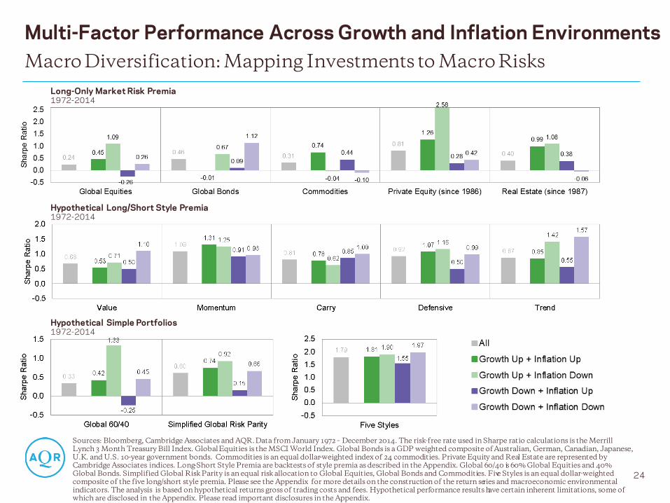
Multi-Factor Performance Across Growth and Inflation Environments
24
Macro Diversification: Mapping Investments to Macro Risks
Sources: Bloomberg, Cambridge Associates and AQR. Data from January 1972 – December 2014. The risk-free rate used in Sharpe ratio calculations is the Merrill Lynch 3 Month Treasury Bill Index. Global Equities is the MSCI World Index. Global Bonds is a GDP weighted composite of Australian, German, Canadian, Japanese, U.K. and U.S. 10-year government bonds. Commodities is an equal dollar-weighted index of 24 commodities. Private Equity and Real Estate are represented by Cambridge Associates indices. Long-Short Style Premia are backtests of style premia as described in the Appendix. Global 60/40 is 60% Global Equities and 40% Global Bonds. Simplified Global Risk Parity is an equal risk allocation to Global Equities, Global Bonds and Commodities. Five Styles is an equal dollar-weighted composite of the five long/short style premia. Please see the Appendix for more details on the construction of the return series and macroeconomic environmental indicators. The analysis is based on hypothetical returns gross of trading costs and fees. Hypothetical performance results have certain inherent limitations, some of which are disclosed in the Appendix. Please read important disclosures in the Appendix.
Long-Only Market Risk Premia 1972-2014
Hypothetical Long/Short Style Premia 1972-2014
Hypothetical Simple Portfolios 1972-2014

Real-World Considerations
Each investor’s chosen recipe will be determined by beliefs and constraints
Typical return and correlation assumptions (including ours) would imply large allocations to alternative risk premia, but it is likely to be only a small part of the solution
Why?
• Conviction: investor uncertainty about the sustainability of other premia than equity
• Constraints: aversion to leverage, shorting and derivatives
• Conventionality: “better to fail conventionally” —Keynes
• Capacity: limitations may apply especially for very large investors
Many investors choose (or are constrained to) long-only implementations
Harvest known return sources efficiently, then add unique alpha if you can find it!
25
Source: AQR.
Investor Constraints Limit the Use of Diversifying Alternatives

TDF: How Traditional TDFs Work
26
Equity Exposure Decreases Through Time
Source: AQR. *Averaged glide path allocations from Fidelity, Vanguard and T Rowe Price Fund Weights as of June 2014. While we show averages, it’s worth noting that there are not substantial differences in the recommendations across the three firms.
As participants age, their risk tolerance decreases
• Most TDFs thus glide from an equity-heavy portfolio to a more capital “balanced” portfolio
0%
20%
40%
60%
80%
100%
40 35 30 25 20 15 10 5 0
%
All
oc
ati
on
Years to Retirement
U.S. Equities International Equities
U.S. Bonds International Bonds
Commodities Cash
0%
2%
4%
6%
8%
10%
12%
14%
40 35 30 25 20 15 10 5 0F
ore
ca
ste
d A
nn
ua
l Vo
lati
lity
Years to Retirement
Traditional Recommended Asset Allocation vs. Years to Retirement*
Estimated Annual Volatility of Recommended Asset Allocation vs. Years to Retirement

MODEL Risk Parity Strategy**
• Constructs GDP-weighted portfolios for global equities and bonds, and equal weighted portfolio for Commodities
• Estimates the risk of each asset class using rolling volatilities
• Combines asset classes to have portfolio with equal volatility contributions from each
• Targets a volatility equal to the expected volatility of the corresponding traditional portfolio at that point in time
• Imposes a leverage constraint on each asset class of 200%
• Net of estimated T-Costs
TDF: Comparing Two Different Approaches to a Glide Path
27
Traditional Vs. Risk Parity
MODEL Traditional Strategy
• Uses allocations from average glide path of largest three providers *
• Holds almost exclusively stocks and bonds
• Reduces equity allocation from ~90% at outset, to ~50% near retirement
• Volatility glides from 12.7% down to 8.1%
• Gross of T-Costs
Source: AQR. *Averaged glide path allocations from Fidelity, Vanguard and T Rowe Price Fund Weights as of June 2014. While we show averages, it’s worth noting that there are not substantial differences in the recommendations across the three firms. **Please see appendix for additional details on t cost assumptions.

TDF: Comparison Methodology
28
A Multi-Cohort Comparison Over a Century
Source: AQR. *While we have over 100 years of data, we should note that we have less than three independent / non-overlapping observations. For further detail see Balancing on the Life Cycle: Target-Date Funds Need Better Diversification (Dhillon, Ilmanen, Liew, 2015)
• We use monthly returns from January 1900 through December 2014, with the first 3 years for risk estimates
• Cohorts are 40 years, with the first cohort ending in December 1942, rolling forward each year
• In this manner, we track 73 investor cohorts, with 40-year life-cycle strategies*
• Savings strategy begins by $1,000 in December, growing by 2.8% real each year, peaking at $3,000 in real terms
• Portfolio risk is reduced over time by either adjusting the equity/bond weights (traditional) or by targeting lower volatility (risk parity)
• The final example of the main text focuses not on ‘revolution’ (fully switch TDF to risk parity plus trend following) but on ‘evolution’ (partial shift: 20% of a portfolio to risk-diversifying alternatives)

29
Antti Ilmanen, Principal, Portfolio Solutions Group
Antti Ilmanen, a Principal at AQR, manages the Portfolio Solutions Group, which advises institutional investors and sovereign wealth funds, and develops AQR’s broad investment ideas. Before AQR, Antti spent seven years as a senior portfolio manager at Brevan Howard, a macro hedge fund, and a decade in a variety of roles at Salomon Brothers/Citigroup. He began his career as a central bank portfolio manager in Finland. Antti earned a Ph.D. in finance from the University of Chicago and M.Sc. degrees in economics and law from the University of Helsinki. Over the years, he has advised many institutional investors, including Norway’s Government Pension Fund Global and the Government of Singapore Investment Corporation. Antti has published extensively in finance and investment journals and has received the Graham and Dodd award and the Bernstein Fabozzi/Jacobs Levy award for his articles. His book Expected Returns (Wiley, 2011) is a broad synthesis of the central issue in investing.
Today’s Presenter

Methodology for Macroeconomic Sensitivity Analysis
Macro Indicators
Each of our macro indicators combines two series, which are first normalized to Z–scores: that is, we subtract a historical mean from each observation and divide by a historical volatility. When we classify our quarterly 12–month periods into, say, ‘growth up’ and ‘growth down’ periods, we compare actual observations to the median so as to have an equal number of up and down observations (because we are not trying to create an investable strategy where data should be available for investors in real time, we use the full sample median).
The underlying series for our growth indicator are the Chicago Fed National Activity Index (CFNAI) and the “surprise” in industrial production growth over the past year. Since there is no uniquely correct proxy way to capture “growth,” averaging may make the results more robust and signals appropriate humility. CFNAI takes this averaging idea to extremes as it combines 85 monthly indicators of U.S. economic activity. The other series – the difference between actual annual growth in industrial production and the consensus economist forecast a year earlier – is narrower but more directly captures the surprise effect in economic developments. We use median forecasts from the Survey of Professional Forecasters data as published by the Philadelphia Fed. While data surprises a priori have a zero mean, this series has exhibited a downward trend in recent decades, reflecting the (partly unexpected) relative decline of the U.S. manufacturing sector.
Note that our growth indicator is constructed from fundamental economic data, rather than asset market returns. Market–based proxies of economic growth – which might include equity market returns, the relative performance of cyclical industries, dividend swaps, and estimates from cross–sectional regressions of asset returns on growth surprises – are “too close” to the patterns we try to explain. Our choice brings its own challenges: macroeconomic data are backward-looking, published with lags and later revised, while asset prices are clearly forward-looking. The impact of publication lags and the mismatch between backward- and forward-looking perspectives can be mitigated by using longer windows. Thus, we use contemporaneous annual economic data and asset returns through our analysis (past-year data with quarterly overlapping observations). Arguably composite growth surprise indices are the best proxies of economic growth news, but such composites are available at best from the1990s. Forecast changes in economist surveys as well as business and consumer confidence surveys may be the next best choices because they ar e reasonably forward-looking and timely. We focus on U.S. data, which have the longest histories. Finally, it is not clear how real economic growth ties to expected corporate cash flow growth (e.g., earnings per share) that influence stock prices, or to real yields that influence all asset prices but especially those of bonds.
Our inflation indicator is also an average of two normalized series. One series measures the de–trended level of inflation (CPIYOY minus its mean, divided by volatility), while the other measures the surprise element in realized inflation (CPIYOY minus consensus economist forecast a year earlier).
Investment Return Series
The investment return series we study include both asset class premia and style premia. The former are long-only returns but expressed in excess returns over the Treasury bill rate. The latter are long-short returns and scaled to target or realize 10% annual volatility. We subtract no trading costs or fees, which makes a bigger difference for the long-short strategies.
The asset class premia are global equities (MSCI World), global bonds (GDP-weighted average of 10-year government bonds in six countries), and an equal-weighted composite of 24 commodity futures.
The market-neutral style premia (Value, Momentum, Carry and Defensive) are hypothetical long/short strategies applied in multiple asset classes: stock selection, industry allocation, country allocation in equity, fixed income and currency markets, and commodities. Each style premia strategy allocates 50/50 risk weights to stock and industry selection (SS) and asset allocation (AA) strategies. For AA we use the same relative risk weights for asset classes as “Investing With Style” (AQR white paper, 2012, available upon request): 33% equity country allocation, 25% fixed income, 25% currencies, 17% commodities. We combine several data sources to produce a dataset long enough to capture many different macroeconomic environments:
• Since 1990, we use value, momentum, carry and defensive style premia strategies as described in “Investing With Style” (AQR white paper, 2012, available upon request). For SS value, momentum and carry we use 50/50 risk weights between stock selection within industries and across industries (to be in line with the common but arguably inefficient practice of letting across-industry positions matter as much as within-industry positions). For SS carry (not included in the white paper) we use the dividend yield strategy returns in Ken French’s data library.
• For 1972-1989, we source value and momentum style returns from “Value and Momentum Everywhere” (Journal of Finance, 2013), defensive style returns from “Betting Against Beta” (Journal of Financial Economics, 2013), and SS carry from the dividend yield strategy returns in Ken French’s data library. We construct the AA carry style premia before 1990 as well as some early histories of AA value, momentum and defensive styles using AQR in-house backtests. These backtests are similar to those described above, but over a narrower universe.
While the SS style premia proxies we use since 1990 are beta-neutral, the value and momentum premia before 1990, and the SS carry premium throughout, are ‘only’ dollar-neutral and may contain moderate empirical beta exposures. The defensive style premia are beta-neutral throughout (we buy larger amounts of low-risk investments than we sell high-risk investments), which means that they are actually not as ‘defensive’ as a dollar-neutral defensive style.
In addition to the four market-neutral style premia, we include the market-directional Trend style, which applies 12-month trend-following strategies in four asset classes: equities, fixed income, currencies and commodities. While the style is nearly uncorrelated with equity markets in the long run, at any point in time it can be directionally long or short. For data since 1985, we use “Time Series Momentum” (Journal of Financial Economics, 2012). For 1972-1984, we use in-house backtests based on the same asset classes, but including 1-, 3- and 12-month momentum, and starting with a smaller asset universe that grows during the period as more assets become available.
30

Construction of Trend-Following Strategy
Trend-Following Strategy The Trend-Following Strategy was constructed with an equal-weighted combination of 1-month, 3-month, and 12-month Trend-Following strategies for 67 markets across 4 major asset classes –29 commodities, 11 equity indices, 15 bond markets, and 12 currency pairs – from January 1880 to June 2015. Since not all markets have return data going back to 1880, we construct the strategies using the largest number of assets for which return data exist at each point in time. We use futures returns when they are available. Prior to the availability of futures data, we rely on cash index returns financed at local short rates for each co untry. In order to calculate net-of-fee returns for the time series momentum strategy, we subtracted a 2% annual management fee and a 20% performance fee from the gross-of-fee returns to the strategy. The performance fee is calculated and accrued on a monthly basis, but is subject to an annual high -water mark. In other words, a performance fee is subtracted from the gross returns in a given year only if the returns in the fund are large enough that the fund’s NAV at the end of the year exceeds every previous end of year NAV. The transactions costs used in the strategy are based on AQR’s 2012 estimates of average transaction costs for each of the four a sset classes, including market impact and commissions. The transaction costs are assumed to be twice as high from 1993 to 2002 and six times as high from 1880–1992, based on Jones (2002). The transaction costs used are as follows: The 2014 estimate of assets under management in the BarclayHedge Systematic Traders index is $280 billion. We looked at the average monthly holdings in each asset class (calculated by summing up the absolute values of holdings in each market within an asset class) for our time series momentum strategy since 2000, run at a NAV of $280 billion, and compared them to the size of the underlying cash or derivative markets. For equities, we use the total global equity market capitalization estimate from the October 2014 World Federation of Exchanges (WFE) monthly statistics tables. For bonds, we add up the total government debt for the 15 deve loped countries with the largest debt using Bloomberg data. For currencies, we use the total notional outstanding amount of foreign exchange derivatives, excluding optio ns, which are U.S. dollar denominated in the first half of 2014 from the Bank for International Settlements (BIS) November 2014 report. For commodities, we use the total notion al of outstanding OTC commodities derivatives, excluding options, in the first half of 2014 from the BIS November 2014 report and add the aggregate exchange futures open in terest for 31 of the most liquid commodities.
31

32
This document has been provided to you solely for information purposes and does not constitute an offer or solicitation of an offer or any advice or recommendation to purchase any securities or other
financial instruments and may not be construed as such. The factual information set forth herein has been obtained or derived from sources believed to be reliable but it is not necessarily all-inclusive
and is not guaranteed as to its accuracy and is not to be regarded as a representation or warranty, express or implied, as to the information’s accuracy or completeness, nor should the attached
information serve as the basis of any investment decision. This document is intended exclusively for the use of the person t o whom it has been delivered and it is not to be reproduced or redistributed to
any other person.
There is no guarantee, express or implied, that long-term return and/or volatility targets will be achieved. Realized returns and/or volatility may come in higher or lower than expected. PAST
PERFORMANCE IS NOT A GUARANTEE OF FUTURE PERFORMANCE. Diversification does not eliminate the risk of experiencing investment losses.
Hypothetical performance results (e.g., quantitative backtests) have many inherent limitations, some of which, but not all, are described herein. No representation is being made that any fund or account
will or is likely to achieve profits or losses similar to those shown herein. In fact, there are frequently sharp differences between hypothetical performance results and the actual results subsequently
realized by any particular trading program. One of the limitations of hypothetical performance results is that they are gener ally prepared with the benefit of hindsight. In addition, hypothetical trading
does not involve financial risk, and no hypothetical trading record can completely account for the impact of financial risk in actual trading. For example, the ability to withstand losses or adhere to a
particular trading program in spite of trading losses are material points which can adversely affect actual trading results. The hypothetical performance results contained herein represent the
application of the quantitative models as currently in effect on the date first written above and there can be no assurance t hat the models will remain the same in the future or that an application of the
current models in the future will produce similar results because the relevant market and economic conditions that prevailed during the hypothetical performance period will not necessarily recur. There
are numerous other factors related to the markets in general or to the implementation of any specific trading program which cannot be fully accounted for in the preparation of hypothetical performance
results, all of which can adversely affect actual trading results. Discounting factors may be applied to reduce suspected anomalies. This backtest’s return, for this period, may vary depending on the
date it is run. Hypothetical performance results are presented for illustrative purposes only. In addition, our transaction cost assumptions utilized in backtests , where noted, are based on AQR's
historical realized transaction costs and market data. Certain of the assumptions have been made for modeling purposes and ar e unlikely to be realized. No representation or warranty is made as to the
reasonableness of the assumptions made or that all assumptions used in achieving the returns have been stated or fully considered. Changes in the assumptions may have a material impact on the
hypothetical returns presented. Hypothetical performance is gross of advisory fees, net of transaction costs, and includes the reinvestment of dividends. If the expenses were reflected, the
performance shown would be lower. Where noted, the hypothetical net performance data presented reflects the deduction of a model advisory fee and does not account for administrative expenses a
fund or managed account may incur. Actual advisory fees for products offering this strategy may vary.
Gross performance results do not reflect the deduction of investment advisory fees, which would reduce an investor’s actual r eturn. For example, assume that $1 million is invested in an account with
the Firm, and this account achieves a 10% compounded annualized return, gross of fees, for five years. At the end of five years that account would grow to $1,610,510 before the deduction of
management fees. Assuming management fees of 1.00% per year are deducted monthly from the account, the value of the account at the end of five years would be $1,532,886 and the annualized
rate of return would be 8.92%. For a ten-year period, the ending dollar values before and after fees would be $2,593,742 and $2,349,739, respectively. AQR’s asset based fees may range up to
2.85% of assets under management, and are generally billed monthly or quarterly at the commencement of the calendar month or quarter during which AQR will perform the services to which the fees
relate. Where applicable, performance fees are generally equal to 20% of net realized and unrealized profits each year, after restoration of any losses carried forward from prior years. In addition, AQR
funds incur expenses (including start-up, legal, accounting, audit, administrative and regulatory expenses) and may have redemption or withdrawal charges up to 2% based on gross redemption or
withdrawal proceeds. Please refer to AQR’s ADV Part 2A for more information on fees. Consultants supplied with gross results are to use this data in accordance with SEC, CFTC, NFA or the applicable
jurisdiction’s guidelines.
Performance Disclosures
Performance Disclosures
Broad-based securities indices are unmanaged and are not subject to fees and expenses typically associated with managed accounts or investment funds. Investments cannot be made directly in an index.
There is a risk of substantial loss associated with trading commodities, futures, options, derivatives and other financial instruments. Before trading, investors should carefully consider their financial
position and risk tolerance to determine if the proposed trading style is appropriate. Investors should realize that when trading futures, commodities, options, derivatives and other financial instruments one could lose the full balance of their account. It is also possible to lose more than the initial deposit when trading der ivatives or using leverage. All funds committed to such a trading strategy should
be purely risk capital.
AQR backtests of Value, Momentum, Carry and Defensive theoretical long/short style components are based on monthly returns, undiscounted, gross of fees and transaction costs, excess of a cash
rate proxied by the Merrill Lynch 3-Month T-Bill Index, and scaled to 12% annualized volatility. Each strategy is designed to take long positions in the assets with the strongest style attributes and short
positions in the assets with the weakest style attributes, while seeking to ensure the portfolio is market-neutral. Please see below for a description of the Universe selection.
Stock and Industry Selection: approximately 2,000 stocks across Europe, Japan, and U.S. Country Equity Indices: Developed Markets: Australia, Canada, Eurozone, Hong Kong, Japan, Sweden,
Switzerland, U.K., U.S. Within Europe: Italy, France, Germany, Netherlands, Spain. Emerging Markets : Brazil, China, India, Israel, Malaysia, Mexico, Poland, Singapore, South Africa, South Korea,
Taiwan, Thailand, Turkey. Bond Futures: Australia, Canada, Germany, Japan, U.K., U.S. Yield Curve: Australia Germany, United States. Interest Rate Futures: Australia, Canada, Europe (Euribor),
U.K. and U.S. (Eurodollar). Currencies: Developed Markets: Australia, Canada, Euro, Japan, New Zealand, Norway, Sweden, Switzerland, U.K., U.S. Emerging Markets: Brazil, Hungary, India, Israel,
Mexico, Poland, Singapore, South Africa, South Korea, Taiwan, Turkey. Commodity Selection: Silver, copper, gold, crude, Brent oil, natural gas, corn, soybeans.
AQR Capital Management (Europe) LLP, a U.K. limited liability partnership, is authorized by the U.K. Financial Conduct Authority (“FCA”) for advising on investments (except on Pension Transfers and
Pension Opt Outs), arranging (bringing about) deals in investments, dealing in investments as agent, managing a UCITS, managing an unauthorized AIF and managing investments. This material has
been approved to satisfy UK FCA COBS 4.
33


