© 2015 R. Sungchasit, P. Pongsumpun and I.M. Tang. This open access article is distributed under a Creative Commons
Attribution (CC-BY) 3.0 license.
American Journal of Applied Sciences
Original Research Paper
SIR Transmission Model of Dengue Virus Taking Into
Account Two Species of Mosquitoes and an Age Structure in
the Human Population
1R. Sungchasit,
1P. Pongsumpun and
2,3I.M. Tang
1Department of Mathematics, Faculty of Science, King Mongkut’s Institute of Technology Ladkrabang,
Chalongkrung Road, Ladkrabang, Bangkok, 10520, Thailand 2Department of Materials Science, Faculty of Science, Kasetsart University, 50 Ngam Wong Wan Road,
Lat Yao Chatuchak, Bangkok 10900, Thailand 3Department of Physics, Faculty of Science, Mahidol University, Rama 6 road, Bangkok 10400, Thailand
Article history
Received: 30-07-2014
Revised: 10-05-2015
Accepted: 22-06-2015
Corresponding Author:
P. Pongsumpun
Department of Mathematics,
Faculty of Science, King
Mongkut’s Institute of
Technology Ladkrabang,
Chalongkrung Road,
Ladkrabang, Bangkok, 10520,
Thailand
Email: [email protected]
Abstract: Dengue is a vector-borne disease. It is transmitted to humans by
the bites of the Aedes aegypti and Aedes albopictus mosquitoes. The human
population is separated into two classes, a child class and an adult class,
each class being described by a SIR model. The transmission rates of the
two mosquito species are different and depend on what class the humans
belong to. We develop a single model taking into account the presence of
two type of mosquitoes and two age classes and apply it to dengue fever.
The model shows how it is possible for the maximum level of infected
human to be reached in a short time. The nature of stability of the
equilibrium state and the trajectories of the individual classes in the model
are determined by the values of the basic reproduction number by setting
the values of the parameters in the model to different values which reflect
the environment in which the epidemic is occurring in the model.
Keywords: Aedes Aegypti, Aedes Albopictus, Dengue Disease, Endemic
Disease State, Equilibrium State, SIR Model
Introduction
Dengue fever is regarded as a serious infectious disease that risks about 2.5 billion people around the world, especially in tropical countries. It is a major epidemic disease occurred in Southeast Asia. Such epidemic arises due to climate change, knowledge of
people and awareness on dengue fever so as to the dengue fever possibly become an endemic for a long time. Moreover, World Health Organization (WHO) (WHO, 2009) estimated 50 to 100 million cases worldwide. About 500,000 people are estimated to be infected by dengue hemorrhagic fever each year.
Dengue fever is caused by four serotypes and they are closely related as a family of dengue virus 1 (DEN 1), virus 2 (DEN2), virus 3 (DEN3) and virus 4 (DEN4). There are viruses carried by two kinds of mosquitoes such as Aedes aegypti and Aedes albopictus. This disease is transmitted to the human though biting of mosquitoes. Recently, It was detected in Asia. However, Aedes aegypti is still the principal vector of dengue fever transmission. Another interesting fact is the shift of patients’ phenomena where dengue fever previously attacks children of primary school age, but now everybody is
vulnerable to fever (Pongsumpun and Tang, 2001; Syafruddin and Noorani, 2012).
Dengue virus is transmitted between the human by biting of an infected Aedes mosquito. When a vector bites someone who be infected with dengue virus, the virus is transferred to mosquitoes and it become infected mosquito. After the infected vector bites the susceptible human, then the virus move into the human bloodstream and it spreads throughout the body. Usually, the mosquitoes bite susceptible people during the day time. Dengue fever is the most common disease in urban areas. The outbreaks commonly occur during the rainy season when the mosquitoes heavily breed in standing water. The dengue fever cases are increasing worldwide. The complications of the disease are leading cases of serious illness and most death in children (Kerpaninch et al., 2001; Kabilan et al., 2003; Malhotra et al., 2006; Wiwanitkit, 2006; Pongsumpum, 2011; Joshi et al., 2002; Koenraadt et al., 2007). One of the major public health problems in many tropical and subtropical regions where Aedes aegypti and Aedes albopictus are present.

R. Sungchasit et al. / American Journal of Applied Sciences 2015, 12 (6): 426.444
DOI: 10.3844/ajassp.2015.426.444
427
It is noted that Aedes albopictus was the principal
vector in the 1940 s outbreaks in Japan (Hotta, 1998),
whereas, Aedes aegypti is commonly the principal
dengue vector in the tropical and subtropical regions.
Aedes aegypti is highly domesticated and exhibits
strong anthropophilia.
Traditional modeling in epidemiology focus on
stability equilibria, since this characterizes if a disease
will become endemic and this is a major concern for
public health officers. The concept of a basic
reproductive number (R0) was introduced and became
a modeling paradigm (Smith et al., 2012) for a very
recent review on the works by Ross and Macdonald
from a medical modeling point of view. In a fairly
large class of models, we can define R0
unambiguously and it can be shown that if R0<1, the
disease is extinct while if R0 >1 it becomes endemic
(Diekmann and Heesterbeek, 2000).
Hence, in this study, we analyze the SIR
(Susceptible-Infected-Recovered) equations for
human and SI (Susceptible-Infected) equations for
mosquitoes. The model will apply empirically on data
of dengue patients reports by Ministry of Public
Health, Thailand (2002-2012) as shown in Fig. 1. The
purpose of this paper is to study the age structural
model of dengue disease incorporated the influence of
Aedes aegypti and Aedes albopictus.
Mathematical Model
The SIR and SI simulates the spread of dengue virus
between host and vector populations. The model is based
on the Susceptible, Infected and Recovered (SIR) model
of infected disease epidemiology, which was adopted by
(Nuraini et al., 2007; Yaacob, 2007). The age structure is
introduced into a model, i.e., children and adults, then
we modify it by incorporating the different behaviors
of Aedes aegypti and Aedes albopictus. In Fig. 1, we
show the age distribution of the incidence rates in one
province in Thailand during 2002-2012 epidemic. As
we see, most cases occur in children under the age of
15. However, a small number of cases do occur in
older people. Similar distributions are seen in the
other provinces in the country.
This model with age structure, the dynamics of each
component of the human is given by:
1 1
(1 sin )
(1 sin )
cc tc ac a
va c bc b vb c d c
dSP N t
dt
I S t I S S
β α ε
β α ε µ
= − +
− + − (1a)
11 1 1 1(1 sin )c
ac a va c c c d c
dIt I S I I
dtβ α ε κ µ= + − − (1b)
21 2 2 2(1 sin )c
bc b vb c c c d c
dIt I S I I
dtβ α ε κ µ= + − − (1c)
1 1 2 2c
c c c c d c
dRI I R
dtκ κ µ= + − (1d)
2 2
(1 sin )
(1 sin )
aa ta aa a
va a ba b vb a d a
dSP N t
dt
I S t I S S
β α ε
β α ε µ
= − +
− + − (1e)
11121 -)sin1( adaaavaaaa
a IISItdt
dIµκεαβ −+= (1f)
22 2 2 2(1 sin )a
ba b vb a a a d a
dIt I S I I
dtβ α ε κ µ= + − − (1g)
1 1 2 2a
a a a a d a
dRI I R
dtκ κ µ= + − (1h)
where the variables and parameters are defined in Table 1.
Fig. 1. Age distribution of the 2002-2012 Dengue fever incidence rates in Thailand

R. Sungchasit et al. / American Journal of Applied Sciences 2015, 12 (6): 426.444
DOI: 10.3844/ajassp.2015.426.444
428
Table 1. Parameters for equations (1a)-(1h) and their definitions
Variable/parameter Definition
Sc, Ic1, Ic2, Rc The numbers of susceptible children, infected from Aedes
aegypti and Aedes albopictus in children and recovered children
Sa, Ia1, Ia2, Ra The numbers of susceptible adult, infected from Aedes aegypti and
Aedes albopictus in adult and recovered adult
Nt The total population
Ntc and Nta The total population in children and the total population in adult they are constant variables
Pc and Pa The birth rate of children and adult human
βac The transmission probability of dengue virus from Aedes aegypti to children
βbc The transmission probability of dengue virus from Aedes albopictus to children
βaa The transmission probability of dengue virus from Aedes aegypti to adult
βba The transmission probability of dengue virus from Aedes albopictus to adult
κc1 The rate at which the infected children from Aedes aegypti can recover
κc2
The rate at which the infected children from Aedes albopictus can recover
κa1 The rate at which the infected adult from Aedes aegypti can recover
κa2 The rate at which the infected adult from Aedes albopictus can recover
µd The natural death rate of human
aa The measure of influence on the transmission process from Aedes aegypti mosquito to human
ab The measure of influence on the transmission process from Aedes albopictus to human
ρva The measure of influence on the transmission process from Aedes aegypti to human
ρvb The measure of influence on the transmission process from Aedes albopictus to human
It we add Equation (1a) – (1h) together, we get:
1 2 1 2( ) ( )
t tc ta
c c c c a a a a
dN dN dN
dt dt dt
S I I R S I I R
= +
= + + + + + + +
The total children and adult populations are supposed to
have constant sizes, i.e., 0tcdN
dt= and 0tadN
dt= , the birth
rate would have to be equivalent to the death rate,
c a dP P µ= = in children and adult, respectively.
where, tcN is the total number of children and is
equivalent to 1 2c c c cS I I R+ + + ,
taN , the total population
in adult and is equal to 1 2a a a aS I I R+ + + .
The dynamics of mosquitoes is described by:
11 1 1 1(1 sin )
a a
vav va va c va v va
dSA t I S S
dtλ ρ ε µ= − + − (2a)
11 1 1 1(1 sin )
a
vava va c va v va
dIt I S I
dtλ ρ ε µ= + − (2b)
22 1 2 2(1 sin )
a a
vav va va a va v va
dSA t I S S
dtλ ρ ε µ= − + − (2c)
22 1 2 2(1 sin )
a
vava va a va v va
dIt I S I
dtλ ρ ε µ= + − (2d)
11 2 1 1(1 sin )
b b
vbv vb vb c vb v vb
dSA t I S S
dtλ ρ ε µ= − + − (2e)
11 2 1 1(1 sin )
b
vbvb vb c vb v vb
dIt I S I
dtλ ρ ε µ= + − (2f)
22 2 2 2(1 sin )
b b
vbv vb vb a vb v vb
dSA t I S S
dtλ ρ ε µ= − + − (2g)
22 2 2 2(1 sin )
b
vbvb vb a vb v vb
dIt I S I
dtλ ρ ε µ= + − (2h)
where, the variable and parameters are given in Table 2.
If we add Equation (2a)-(2h) together, we get:
1 11
( )a a
va vav v va
d S IA N
dtµ+
= − (3a)
2 22
( )a a
va vav v va
d S IA N
dtµ+
= − (3b)
1 11
( )b b
vb vbv v vb
d S IA N
dtµ+
= − (3c)
2 22
( )b b
vb vbv v vb
d S IA N
dtµ+
= − (3d)
where,
1vaN and 2vaN are the numbers of Aedes aegypti
in children and adult respectively, which is equal to
Sva1+Iva1 and Sva2 + Iva2. Nvb1 and Nvb2 are the numbers of
Aedes albopictus in children and adult respectively,
which is equal to Svb1 + Ivb1 and Svb2 + Ivb2. If the
numbers of mosquitoes are also constant each other (3a)-
(3d) gives 1 /a ava v vN A µ= , 2 /
a ava v vN A µ= , 1 /b bvb v vN A µ=
and 2 /b bvb v vN A µ= .

R. Sungchasit et al. / American Journal of Applied Sciences 2015, 12 (6): 426.444
DOI: 10.3844/ajassp.2015.426.444
429
Table 2. Parameters for equations (2a)-(2g) and their definitions
Variable/ parameter Definition
Sva1 and Iva1 The number of susceptible and infected Aedes aegypti mosquitoes who be infected from children
avµ The death rate of Aedes aegypti mosquito
avA The carrying capacity of the environment for Aedes aegypit
λva1 The probability that a dengue virus transmitted to the Aedes aegypti from an infected children
Sva2 and Iva2 The number of susceptible and infected Aedes aegypti mosquitoes who be infected from adult
avµ The death rate of Aedes aegypti mosquito
avA The carrying capacity of the environment for Aedes aegypit mosquito
λva2 The probability that a dengue virus transmitted to the Aedes aegypti from an infected adult human
Svb1 and Ivb1 The number of susceptible and infected Aedes albopictus mosquitoes who be infected from children
bvµ The death rate of Aedes albopictus mosquito
bvA The carrying capacity of the environment for Aedes albopictus mosquito
λvb1 The probability that a dengue virus transmitted to the Aedes albopictus from an infected human in children
Svb2and Ivb2 The number of susceptible and infected Aedes albopictus mosquitoes who be infected from adult human
bvµ The death rate of Aedes albopictus mosquito
bvA The carrying capacity of the environment for Aedes albopictus mosquito
λvb2 The probability that a dengue virus transmitted to the Aedes albopictus from an infected adult
We normalize parameter (1a)-(1h) and (2a)-(2h) by
writing cc
tc
SS
N′ = , 1
1c
c
tc
II
N′ = , 2
2c
c
tc
II
N′ = , c
c
tc
RR
N′ = in children
and aa
ta
SS
N′ = , 1
1a
a
ta
II
N′ = , 2
2a
a
ta
II
N′ = , a
a
ta
RR
N′ = in adult.
11
1
vava
va
SS
N′ = , 1
1
1
vava
va
II
N′ = , 2
2
2
vava
va
SS
N′ = , 2
2
2
vava
va
II
N′ = ,
11
1
vbvb
vb
SS
N′ = , 1
1
1
vbvb
vb
II
N′ = , 2
2
2
vbvb
vb
SS
N′ = and 2
2
2
vbvb
vb
II
N′ = , then the
reduced equations become:
1 1 1 1
(1 sin )
(1 sin )
c d ac a
va va c bc b vb vb c d c
dS t
dt
I N S t I N S S
µ β α ε
β α ε µ
′ = − +
′ ′ ′ ′ ′− + − (4a)
1 1 1 1 1 1(1 sin )c ac a va va c c c d c
dI t I N S I I
dtβ α ε κ µ′ ′ ′ ′ ′= + − − (4b)
2 1 1 2 2 2(1 sin )c bc b vb vb c c c d c
dI t I N S I I
dtβ α ε κ µ′ ′ ′ ′ ′= + − − (4c)
2 2 2 2
(1 sin )
(1 sin )
a d aa a
va va a ba b vb vb a d a
dS t
dt
I N S t I N S S
µ β α ε
β α ε µ
′ = − +
′ ′ ′ ′ ′− + − (4d)
1 2 2 1 1 1(1 sin )a aa a va va a a a d a
dI t I N S I I
dtβ α ε κ µ′ ′ ′ ′ ′= + − − (4e)
2 2 2 2 2 2(1 sin )a ba b vb vb a a a d a
dI t I N S I I
dtβ α ε κ µ′ ′ ′ ′ ′= + − − (4f)
1 1 1 1 1(1 sin )ava va va c tc va v va
dI t I N S I
dtλ ρ ε µ′ ′ ′ ′= + − (4g)
2 2 1 2 2(1 sin )ava va va a ta va v va
dI t I N S I
dtλ ρ ε µ′ ′ ′ ′= + − (4h)
1 1 2 1 1(1 sin )bvb vb vb c tc vb v vb
dI t I N S I
dtλ ρ ε µ′ ′ ′ ′= + − (4i)
2 2 2 2 2(1 sin )bvb vb vb a ta vb v vb
dI t I N S I
dtλ ρ ε µ′ ′ ′ ′= + − (4j)
Where:
1 2 1 2
1 1 2 2 1 1 2 2
1, 1,
1, 1, 1 1
c c c c a a a a
va va va va vb vb vb vb
S I I R S I I R
S I S I S I and S I
′ ′ ′ ′ ′ ′ ′ ′+ + + = + + + =′ ′ ′ ′ ′ ′+ = + = + = + =
Mathematical Analysis
Equilibrium States
The equilibrium states * * * * * * * * * *
1 2 1 2 1 1 2 2( , , , , , , , , , )
c c c a a a va vb va vbS I I S I I I I I I are obtained by
setting the right hand side of (4a)-(4j) to zero.
Therefore we obtain * * * * *
1 2 1 1( , , , , )
c c c va vbS I I I I and * * * * *
1 2 2 2( , , , , )
a a a va vbS I I I I . Doing this,
we get four equilibrium states.
A. The two group disease free equilibrium state:
( )0E = 1, 0, 0, 1, 0, 0, 0, 0, 0, 0
A1.the disease free equilibrium state:
( )* * * * *
oc c c1 c2 va1 vb1E =( S ,I ,I , I ,I )= 1, 0, 0, 0, 0 in children
A2.the disease free equilibrium state:

R. Sungchasit et al. / American Journal of Applied Sciences 2015, 12 (6): 426.444
DOI: 10.3844/ajassp.2015.426.444
430
( )* * * * *
0a a a1 a2 va2 vb2E =(S ,I ,I ,I ,I )= 1, 0, 0, 0, 0 in adult
B. The two group endemic equilibrium state:
),,,,,,,,,(ˆ *2
*2
*2
*1
**1
*1
*2
*1
*vbvaaaavbvaccc IIIISIIIISE =
B1.the endemic state:
* * * * *
1c c c1 c2 va1 vb1E = ( S , I , I ,I ,I ) in children
Where:
1 2 1
1*
* *
1 1 1 1 1 1
1
( ( )
sin )
( ( (
)sin )(1 sin )))
t c d v b c d vb
tc d vb v b
c
t c v b v a v a ac v b b c d v a va
a a c v b b bc v b
N
N tS
N I N N I N
N t t
µ λ κ µ µ
µ λ ρ ελ β β µ
α β α β ε ρ ε
+ +
+=
+ + +
+ +
(5a)
*
1 1 1
2 1*
1 *
1 1 1 1 1
*
1 1 1
(1 sin )(
( ) sin ))
( ( )(
( ) sin ) (1 sin ))
b
va v a ac a tc d vb
c d v tc d vb vb
c
tc vb c d va va ac vb bc d
va v a a ac vb b bc vb
I N t N
N tI
N I N N
I N N t t
β α ε µ λ
κ µ µ µ λ ρ ελ κ µ β β µ
α β α β ε ρ ε
+
+ + +=
+ + + +
+ +
(5b)
*
1 1 1
2 1*
2 * *
1 2 1 1 1 1
*
1 1 1
( (1 sin )(
( ) sin ))
( ( )(
( )sin )(1 sin ))
b
vb vb bc b tc vb d
c d v tc vb d vb
c
tc vb c d va va ac vb vb bc d
va va a ac vb b bc vb
I N t N
N tI
N I N I N
I N N t t
β α ε λ µκ µ µ λ µ ρ ε
λ κ µ β β µ
α β α β ε ρ ε
+
+ + +=
+ + + +
+ +
(5c)
*
1 1 1
1 1 2
1 1 2
1 1 1
1 1 1
1 1 2
1
[(2( 2 ( )
2 ( )
( )
( ) (2 )
(2 ( )))
2( ( )
a
b
b a
b
va vb d c d v
va ac va c d v
va a ac va c d
v va vb bc vb c d v b vb
tc va ac va vb d va vb a va vb
va a ac va c d v va
vb b bc vb
I
N
N
N
N N
N
N
λ µ κ µ µ
β λ κ µ µ
α β λ κ µ
µ ρ β λ κ µ µ α ρ
β λ λ µ ρ ρ α ρ ρ
α β λ κ µ µ ρ
α β λ
= − +
+ +
+ +
− + +
+ + + +
− +
− 1 1
1 1 1
1 1 2
1 1 1 1 1
1 1 1
( )
( ( )))cos
2 (4( ( ) ( )
( ) ( ) ( ))
(4( )
(4 3 )))sin
a
b
a a
c d v vb
tc va ac va vb d va vb a va vb
va ac va c d v a va
vb d c d v vb bc vb c d v b vb
tc va ac va vb d va vb
a va vb
N N
t N
N
N N
t
κ µ µ ρ
β λ λ µ ρ ρ α ρ ρ
ε β λ κ µ µ α ρ
λ µ κ µ µ β λ κ µ µ α ρ
β λ λ µ ρ ρ
α ρ ρ ε
+
+ + +
+ + +
− + − + +
+ +
+ +
1 1 1
1 1 1
1 2 2
1 1 1 1
1 2 1 1
sin )]
/[(2 (1 sin )(2 ( )
2 ( ) ( )
(2 ) cos 2
2( ( ) ( )
a
b b
b b
tc va a ac va vb d va vb
va ac a vb c d v
va c d v c d v
tc d va vb va vb tc d va vb va vb
va c d v va vb c d v vb
tc d
N N t
N t
N N t
N
α β λ λ µ ρ ρ ε
β α ε λ κ µ µ
λ κ µ µ κ µ µ
µ λ λ ρ ρ µ λ λ ρ ρ ε
λ κ µ µ ρ λ κ µ µ ρ
µ λ
−
+ +
+ + +
+ + −
+ + + +
+ 1 1 ( ))sin ))]va vb va vb tλ ρ ρ ε+ (5d)
* *
1 1 1 1 1 2
*
1 1 2
1 1
1 1
1 1
2 1
[( ( )( )
sin ( ( )
( )
sin ))]
/[ (1 sin )(
( ) sin
b
b
b
vb tc vb ac vb d va va ac d c d v
va va a ac c d v
tc vb bc vb d b vb
tc vb b bc vb d vb
vb bc b tc vb d
c d v tc vb d vb
I N N I N
t I N
N N
N N t
N t N
N
β λ µ β µ κ µ µ
ε α β κ µ µ
β λ µ α ρ
α β λ µ ρ ε
β α ε λ µ
κ µ µ λ µ ρ ε
= − + +
+ − +
+ +
+
+
+ + + ))]t
(5e)
B2. The endemic state:
* * * * *
1 1 2 2 2( , , , , )
a a a a va vbE S I I I I in adult=
Where:
2 2 2*
*
2 2 2 2
*
2 2 2
( ( ) sin )
( (
( )sin )(1 sin )))
bta d vb a d v ta d vb vb
a
ta vb va va aa vb ba d
va va a aa vb b ba vb
N N tS
N I N N
I N N t t
µ λ κ µ µ µ λ ρ ελ β β µ
α β α β ε ρ ε
+ + +=
+ +
+ + +
(6a)
*
2 2 2
2 2*
1 *
2 1 2 2 2
*
2 2 2
(1 sin )(
( ) sin ))
( ( )(
( )sin )(1 sin ))
b
va va aa a ta d vb
a d v t a d vb vb
a
ta vb a d va va aa vb ba d
va va a aa v b b ba vb
I N t N
N tI
N I N N
I N N t t
β α ε µ λ
κ µ µ µ λ ρ ελ κ µ β β µ
α β α β ε ρ ε
+
+ + +=
+ + +
+ + +
(6b)
* *
2 2 2 2
2 2
*
2 2 2 2
* *
2 2 2 2
2
[( (1 sin )(
( ) sin ))
/ ( )(
(
)sin )(1 sin ))]
b
a vb vb ba b ta vb d
a d v ta vb d vb
ta vb a d va va aa
vb vb ba d va va a aa
vb b ba vb
I I N t N
N t
N I N
I N I N
N t t
β α ε λ µκ µ µ λ µ ρ ε
λ κ µ β
β µ α β
α β ε ρ ε
= ++ + +
+
+ + +
+ +
(6c)
*
2 2 1 2 2 2
2 2 2
2 2 1
2 2 2
2 2 2
2
[(2( 2 ( ) 2 ( )
( )
( ) (2 )
(2 ( )))
2( ( )
a b
b
a
b
va vb d a d v va aa va a d v
va a aa va a d v va
vb ba vb a d v b vb
ta va aa va vb d va vb a va vb
va a aa va a d v va
vb b ba vb
I N
N
N
N N
N
N
λ µ κ µ µ β λ κ µ µ
α β λ κ µ µ ρ
β λ κ µ µ α ρ
β λ λ µ ρ ρ α ρ ρ
α β λ κ µ µ ρ
α β λ
= − + + +
+ +
− + +
+ + + +
− +
− 2 1
2 2 2
2 2 2
2 1 2 2 1
2 2 2
( )
( ( )))cos2
(4( ( ) ( )
( ) ( ) ( ))
(4( )
(4 3 ))) sin
a
b
a a
a d v vb
ta va aa va vb d va vb a va vb
va aa va a d v a va
vb d a d v vb ba vb a d v b vb
ta va aa va vb d va vb
a va vb
N N t
N
N
N N
t
κ µ µ ρ
β λ λ µ ρ ρ α ρ ρ ε
β λ κ µ µ α ρ
λ µ κ µ µ β λ κ µ µ α ρ
β λ λ µ ρ ρα ρ ρ ε
+
+ + +
+ + +
− + − + +
+ +
+ +
2 2 2
2 2 1
2 2 2 2 2
2 2 2 2
2 1
sin )]
/[(2 (1 sin )(2 ( )
2 ( ) ( ) (2 )
cos2 2( ( )
( )
a
b b
b
a
ta va a aa va vb d va vb
va aa a vb a d v
va a d v a d v ta d va vb va vb
ta d va vb va vb va a d v va
vb a d v vb ta d
N N t
N t
N
N t
N
α β λ λ µ ρ ρ ε
β α ε λ κ µ µ
λ κ µ µ κ µ µ µ λ λ ρ ρ
µ λ λ ρ ρ ε λ κ µ µ ρ
λ κ µ µ ρ µ λ
−
+ +
+ + + + +
− + +
+ + + 2 2 ( ))sin ))]va vb va vb tλ ρ ρ ε+
(6d)

R. Sungchasit et al. / American Journal of Applied Sciences 2015, 12 (6): 426.444
DOI: 10.3844/ajassp.2015.426.444
431
* *
2 2 2 2 2 2
*
2 2 2
2 2
2 2
2 2 2
2
[( ( )( )
sin ( ( )
( )
sin ))]/
[ (1 sin )( ( )
sin
b
b
b
vb ta vb aa vb d va va aa d a d v
va va a aa a d v
ta vb ba vb d b vb
t a vb b ba vb d vb
vb ba b ta vb d a d v
ta vb d vb
I N N I N
t I N
N N
N N t
N t N
N
β λ µ β µ κ µ µ
ε α β κ µ µ
β λ µ α ρ
α β λ µ ρ ε
β α ε λ µ κ µ µ
λ µ ρ ε
= − + +
+ − +
+ +
+
+ + +
+ ))]t
(6e)
Local Asymptotically Stability
The local stability of each equilibrium state is
determined from Jacobian matrix of right hand side of
the above set of differential equations evaluated at the
equilibrium state.
Proposition A. If S0<1, S0c<1 and S0a<1when ε = 0,
then the disease free equilibrium state E0c in children and
E0a in adult are locally asymptotically stable, where:
1 1 1
1 1 1 2
1
1 1 1
1 1 2
1
0
2 ( )
(2( ( ) )
(2 ) 2 ( ))
(2 ( ) (2 (2 ))
2 ( ( )
( ( ) )))max
a
b
a
b
vb b bc vb c d v vb
va ac va tc vb d c d v
a va tc vb d a va
vb c d v d vb bc b vb
va ac va a c d v va
tc vb d a va a va vb
N
N N
N
N
N
NS
α β λ κ µ µ ρ
β λ λ µ κ µ µ
α ρ λ µ α ρλ κ µ µ µ β α ρ
β λ α κ µ µ ρ
λ µ α ρ α ρ ρ
+ +
+ +
+ + ++ + +
+ +
+ + +=
2 2 1
2 2 2 2
2
2 1 2
2 2 2
2
,
2 ( )
(2( ( ) )
(2 ) 2 ( ))
(2 ( ) (2
(2 )) 2 ( ( )
( ( ) )))
a
b
a
b
vb b ba vb a d v vb
va aa va ta vb d a d v
a va ta vb d a va
vb a d v d vb ba
b vb va aa va a a d
v va ta vb d a va a va vb
N
N N
N
N
N
N
α β λ κ µ µ ρ
β λ λ µ κ µ µ
α ρ λ µ α ρλ κ µ µ µ β
α ρ β λ α κ µ
µ ρ λ µ α ρ α ρ ρ
+
+ + +
+ + ++ +
+ + +
+ + +
(6f)
1 1 1
1 1 1 2
10
1 1 1
1 1 2
1
2 ( )
(2( ( ) )
(2 ) 2 ( ))
(2 ( ) (2 (2 ))
2 ( ( )
( ( ) )))
in
a
b
a
b
vb b bc vb c d v vb
va ac va tc vb d c d v
a va tc vb d a vac
vb c d v d vb bc b vb
va ac va a c d v va
tc vb d a va a va vb
N
N N
NS
N
N
N
α β λ κ µ µ ρ
β λ λ µ κ µ µ
α ρ λ µ α ρλ κ µ µ µ β α ρ
β λ α κ µ µ ρ
λ µ α ρ α ρ ρ
+
+ + +
+ + +=
+ + +
+ +
+ + +
children
(6g)
2 2 1
2 2 2 2
2
0
2 1 2
2 2 2
2
2 ( )
(2( (
) )(2 ) 2 ( ))in
(2 ( ) (2 (2 ))
2 ( ( )
( ( ) )))
a
b
a
b
vb b ba vb a d v vb
va aa va ta vb d a
d v a va ta vb d a va
a
vb a d v d vb ba b vb
va aa va a a d v va
ta vb d a va a va vb
N
N N
NS
N
N
N
α β λ κ µ µ ρ
β λ λ µ κ
µ µ α ρ λ µ α ρλ κ µ µ µ β α ρ
β λ α κ µ µ ρ
λ µ α ρ α ρ ρ
+
+ +
+ + + +=
+ + +
+ +
+ + +
adult (6h)
Proof.
For the disease free equilibrium state in children E0c
= (1, 0, 0, 0, 0) and in adult E0a = (1, 0, 0, 0, 0).
The system defined by Equation (4a) - (4j), the
Jacobian matrix evaluated at E0c and E0a respectively,
given by:
1 1
1 1
2 1
1 1
1 1
( ) 0 0 (1 sin ( ))
(1 sin ( ))
0 ( ) 0 (1 sin ( )) 0
0 0 ( ) 0 (1 sin ( ))
0 (1 sin ( )) 0 0
0 0 (1 sin ( )) 0
d a c a
va bc b vb
c d ac a va
c
c d bc b v b
v a v a va
v b v b v b
t
N t N
t NJ
t N
t
t
µ β α ε
β α ε
κ µ β α ε
κ µ β α ε
λ ρ ε µ
λ ρ ε µ
− − +
− +
− + + = − + + + −
+ −
(7a)
2
2
1 2
2 2
2 2
2 2
( ) 0 0 (1 sin ( ))
(1 sin ( ))
0 ( ) 0 (1 sin( )) 0
0 0 ( )0 (1 sin ( ))
0 (1 sin ( )) 0 0
0 0 (1 sin ( ))0
d aa a va
ba b vb
a d aa a vaa
a d ba b vb
va va va
vb vb vb
t N
t N
t NJ
t N
t
t
µ β α ε
β α ε
κ µ β α ε
κ µ β α ελ ρ ε µ
λ ρ ε µ
− − + − + − + + = − + +
+ − + −
(7b)
The eigenvalues are obtained by solving the
characteristic equations, det ηI5-Ji= 0. Where I5 is the
5×5 identity matrix and Ji(Ji; i = c,a) is the Jacobian matrix
matrix for (7a) and (7b), respectively. To evaluate the
determinant, we get the following characteristic equations:
4 3 2
1 2 3 4( )( ) 0
dW W W Wη µ η η η η+ + + + + = (8a)
4 3 2
1 2 3 4( )( ) 0
dF F F Fη µ η η η η+ + + + + = (8b)
Where:
1 1 2 2a bc c d v vW κ κ µ µ µ= + + + + (9a)
2 1 1 1 1
2
2 1 2
)
2 2
( ) ( )
a b a b
a b a b
va ac va vb bc vb
d d v d v v v
c d v v c c d v v
W N Nβ λ β λ
µ µ µ µ µ µ µ
κ µ µ µ κ κ µ µ µ
=− −
+ + + +
+ + + + + + +
(9b)
3 1 2 1 1 1
1 2 1 2
1 1 2 1 2
( )( ) ( )
(( )( ) ( 2 ) )
( ) ( ( ))
a a
a
b b b
c d c d v vb bc vb c d v
c d c d c c d v
v va ac va c d v ac va c d v
W N
N
κ µ κ µ µ β λ κ µ µ
κ µ κ µ κ κ µ µ
µ β λ κ µ µ β λ κ µ µ
= + + − + +
+ + + + + +
− + + + + +
(9c)
4 1 1 1
1 1 2
( ( ) )
( ( ) )
a
b
va ac va c d v
vb bc vb c d v
W N
N
β λ κ µ µ
β λ κ µ µ
= − +
+ + (9d)
1 1 2 2a ba a d v vF κ κ µ µ µ= + + + + (9e)
2
2 2 2 2 2
2 1 2
) 2 2
( ) ( )
a b
a b a b a b
va aa va vb ba vb d d v d v
v v a d v v a a d v v
F N Nβ λ β λ µ µ µ µ µ
µ µ κ µ µ µ κ κ µ µ µ
=− − + + +
+ + + + + + + + (9f)

R. Sungchasit et al. / American Journal of Applied Sciences 2015, 12 (6): 426.444
DOI: 10.3844/ajassp.2015.426.444
432
3 1 2 2 2 1
1 2 1 2
2 2 2 2 2
( )( ) ( )
(( )( ) ( 2 ) )
( ) ( ( ))
a a
a b
b b
a d a d v vb ba vb a d v
a d a d a a d v v
va aa va a d v aa va a d v
F N
N
κ µ κ µ µ β λ κ µ µ
κ µ κ µ κ κ µ µ µ
β λ κ µ µ β λ κ µ µ
= + + − + +
+ + + + + +
− + + + + +
(9g)
4 2 2 1 2 2 2( ( ) )( ( ) )a bva aa va a d v vb ba vb a d vF N Nβ λ κ µ µ β λ κ µ µ= − + + + (9h)
From the characteristic equation, Equation (8a)-(8b),
we see that eigenvalues are c dη µ=− and
a dη µ=− , all of
these eigenvalues are negative, for 0
1S < . The sign of
other four eigenvalues can be ascertained by solving
equation 4 3 2
1 2 3 4( ) 0W W W Wη η η η+ + + + = and
4 3 2
1 2 3 4( ) 0F F F Fη η η η+ + + + = . The remaining four
eigenvalues have negative real parts if they satisfy
Routh-Hurwitz criteria (10a) - (10d) (Esteva and Vargas,
1998), each equilibrium state is locally asymptotically
stable if the following conditions are satisfied:
1 1 0W and F > (10a)
3 3 0W and F > (10b)
4 4 0W and F > (10c)
2 2
1 2 3 3 1 4 1 2 3 3 1 4( ) 0 ( ) 0WW W W W W and F F F F F F− + > − + > (10d)
After we use Mathematica to show the conditions
of locally asymptotically stable, we can see that W1
and F1 are always positive. For the equations given by
(10b)-(10d), we show these conditions by using the
following Fig. 2.

R. Sungchasit et al. / American Journal of Applied Sciences 2015, 12 (6): 426.444
DOI: 10.3844/ajassp.2015.426.444
433
Fig. 2. The parameter spaces for the disease free equilibrium state, which satisfies the Routh-Hurwitz conditions, show onto
),( 31 Wcκ , ),( 32 Wcκ , ),( 31 Faκ , ),( 32 Faκ , ),( 41 Wcκ , ),( 42 Wcκ , ),( 41 Faκ , ),( 42 Faκ , )))((,( 42
133211 WWWWWWc −−κ ,
)))((,( 42
133211 WWWWWWc −−κ , )))((,( 42
133211 FFFFFFa −−κ , )))((,( 42
133212 FFFFFFa −−κ , respectively. The values of
parameter are follows: )2/17(/11 =cκ , )2/19/(12=cκ , )6.74*365/(1=dµ day−1, 9000=tcN , 40001 =vaN , 55001 =vbN , 00769.0=acβ ,
000246.0=bcβ , 00000576.01 =vaλ , 00000335.01 =vbλ , 07.0=aα , 067.0=bα and 100000=tN , )2/19(/11 =aκ , )2/21/(12 =aκ ,
)6.74*365/(1=dµ day−1, 6000=taN , 30002 =vaN , 41002 =vbN , 000045.0=aaβ , 000067.0=baβ , 0066.02 =vaλ , 00235.02 =vbλ ,
07.0=aα , 067.0=bα and 100000=tN . From the above figures, the Routh-Hurwitz conditions are satisfied for 10 >S

R. Sungchasit et al. / American Journal of Applied Sciences 2015, 12 (6): 426.444
DOI: 10.3844/ajassp.2015.426.444
434
Endemic Disease State
Proposition B. If S0>1, when 0ε = , then the equilibrium
state * * * * * * * * * *
1 2 1 1 1 2 2 2ˆ ( , , , , , , , , , )
c c c va vb a a a va vbS S I I I I S I I I I= is
locally asymptotically stable.
Proof.
For the endemic disease equilibrium
state * * * * *
1 1 2 1 1( , , , , )
c c c c va vbE S I I I I= in children and
* * * * *
1 1 2 2 2( , , , , )
a a a a va vbE S I I I I= in adult, we obtain the
characteristic equation:
5 4 3 2
1 2 3 4 5( ) 0D D D D D in childrenη η η η η+ + + + + = (11a)
5 4 3 2
1 2 3 4 5( ) 0G G G G G in adultη η η η η+ + + + + = (11b)
Where:
1 1 1 1 2 1 2 3a bva ac vb bc c c d v vD N Nβ θ β θ κ κ µ µ µ= + + + + + + (12a)
2
2 1 2 1 2 1 2 1
1 2 1 1
1 1 1 1 2 1 1 2
1 1 1 1 2
1 1 1 1 1
2 2 3
3 ( 3 )
( ( / ) ( 2
( / ) ))
( ( /
a
a b
a b
c c c d c d d c v c va
d v c c d va v va ac
va d va ac vb bc d c c d
va d va ac vb bc d v v
vb bc vb d va ac vb
D
N
N N
N N
N N N
κ κ κ µ κ µ µ κ µ κ µ
µ µ κ κ µ µ µ β
λ µ β θ β θ µ θ κ κ µ
λ µ β θ β θ µ µ µ
β λ µ β θ β
= + + + + +
+ + + + +
− + + + +
+ + + +
+ − + 2 2 1
2 1 1 1 1 2
) (
2 ( / ) ))a b
bc d c
c d vb d va ac vb bc d v vN N
θ µ θ κ
κ µ λ µ β θ β θ µ µ µ
+
+ + + + +
(12b)
2 2 2 2
3 1 1 1
1 1 1 2
2 1 2
2 2 2
1 2
2
2 1 2
2
2
1( ( 2
2 ( ) (
))
( 2 2
( ) (
)) ( ( 2 (
b a b a b
a b
a b
a b a b a
b a b
va ac d d va
va ac vb bc d
d v v v c d v v c c d
v v vb bc
d d v d v
v v c d v v c c d v
v d c d v v d
D NN N
N
β θ µ µ µβ θ β θ µ
µ µ µ µ κ µ µ µ κ κ µ
µ µ β θ
µ µ µ µ µ
µ µ κ µ µ µ κ κ µ µ
µ µ κ µ µ µ µ
= ++ +
+ + + + + + +
+ + +
+ +
+ + + + + + +
+ + + +2 2
1
2 1
1 1 2 2 1
2 1 2
2
))
( 3 3 ( )) (
2 ( ) ( )))
( ( 2 ) ( (2 (
) (3 5 ) ) ( (3 )
(5 4 )) (2
a b
a b a b a b
a b a b
a
a a
a b a
v v
d d v v d v v c d v v
d v v c d v v vb bc
vb d c d v d d c vb
d c vb d v c d v
d d v v c d v
N
µ µ
µ µ µ µ µ µ µ κ µ µ µ
µ µ µ κ µ µ µ β
λ µ κ µ µ θ µ µ κ λ
µ κ λ µ µ κ µ µ
µ µ µ µ κ µ µ
+
+ + + + + +
+ + + + + +
− + + + +
+ + + + + +
+ + + + +
1 1
2 1 2 1
2
1
2
1 1
2
1 2 1 1 1 2
))))
(
( 2 ) ( (
2 3 ) (3 )
(2 ( )
5 ( 5 4 ) ) (2
3 ( ) (2 )))
( ( (
b
b
b a b
a a b a b
a b a b
v
va ac va d
c d v c d va
d v c d v v
d d va d
d v va d v v c d v v
d v v c d v v
vb bc va d vb d
N
N
µ
β λ µ
κ µ µ θ κ µ λ
µ µ κ µ µ µ
µ µ λ µ
µ µ λ µ µ µ κ µ µ µ
µ µ µ κ µ µ µ
β θ λ µ θ λ µ θ
+ −
+ + +
+ + + +
+ +
+ + + + + +
+ + + + +
+ − + − + 1 1
2
1 2
(
2 4 ) 2(2 )
2 ( )
2 ( ))))))
a b b
a b
a b
d va vb
d v d v v
c d v v
c c d v v
µ λ λµ µ µ µ µ
κ µ µ µ
κ κ µ µ µ
+
+ + + +
+ + +
+ + + +
(12c)
2 2 3
4 1 2 1 2 1 2
2 2 3
1 2 1 2 1
3
2
1 1 1 2
2
1 2 1 2 1 1
2
12 3
(( 1 ) ( 2 ) (
a a a a b
b b b a b a b
a b a b
a
c c d v c d v c d v d v c c d v
c d v c d v d v c c v v c d v v
c d v v d v v
va ac vb b c d
vb bc vb d d v va ac
D
N N
N N N
κ κ µ µ κ µ µ κ µ µ µ µ κ κ µ µ
κ µ µ κ µ µ µ µ κ κ µ µ κ µ µ µ
κ µ µ µ µ µ µβ θ β θ µ
β θ λ µ µ µ θ β θ
= + + + +
+ + + + +
+ + ++ +
− + + + + 1 2
2 2 2
1 2 1 2 1 1 1 2 2
2 22 1 1 2 1
2 1
1 1 1 2 1
)
( ( ) ( ( ) ( 2 ) ) )
(( 1 ) ( 2 ) ( ) (( )
( ) ))) (
a a b
a a
a b
vb bc d
d c d v d c d c d v v
c vb d d v va a c vb bc d c d v
c v a d c va dc d v v va ac
va ac vb bc d va
N N
NN N N
β θ µ
µ κ µ µ µ κ µ κ µ µ µ
κ θ λ µ µ µ θ β θ β θ µ κ µ µ
κ λ µ θ κ λ µκ µ µ µ ββ θ β θ µ
+
+ + + + +
+ − + + + + + +
+ + + + − ++ + 1 1 2
3 3
1 1 1
1 1 2 1 1
1 1 1 2 1 1 1 2
2 2
1 2 1 1 1 2 1 1 1 2 1
2 1
1 1 1 2
a a
a a b b b b
b
ac vb bc d
va d v a d
c c v c d v
va ac vb bc d va ac vb bc d
c d v d v c c v c d v c d v d v
c va d v
va ac vb bc
N
N N N N
N N
β θ β θ µ
λ µ θ λ µθ κ κ µ θ κ µ µ
β θ β θ µ β θ β θ µ
θ κ µ µ θ µ µ θ κ κ µ θ κ µ µ θ κ µ µ θ µ µ
κ λ µ µβ θ β θ µ
+ +
− + + ++ + + +
+ + + + + +
−+ +
2 2
1 2 1 1 1 1
1 1 1 2 1 1 1 2 1 1 1 2
1 1 1 2 1 1 1 12
1 1 1 2
1 1
2 2
12 (
( )
( (
b b b
a b a b a b
c va d v va d v v a d v
d va ac vb bc d va ac vb bc d va ac vb bc d
c v v c v v d v v vb bc d va ac
va ac vb bc d
vb
N N N N N N
N NN N
θ κ λ µ µ λ µ µ θ λ µ µβ θ β θ µ β θ β θ µ β θ β θ µ
θ κ µ µ θ κ µ µ θ µ µ µ β µ β θβ θ β θ µ
θ λ κ
+ − ++ + + + + +
+ + + ++ +
−1 2 1 2 .1 1 1 1 1 1
1 2 1 1 1 2 1 2 1 1 1 1 1 1
1 1 1 1 1
) (( 1 ) ( ) ( ( ) ( ))))
( ( ) (( 1 ) ( ) ( ( )
( )))) ( ( (
a b a b
a a
b
c d v c va va d v vb c d v va d v
vb bc vb c d v c va va d vb vb c d v
va d v d vb va c
N
µ µ θ θ κ λ λ µ µ θ λ κ µ µ λ µ µ
β θ θ λ κ µ µ θ θ κ λ λ µ µ θ λ κ µ µ
λ µ µ µ λ λ θ κ λ
+ + + − + − + + + + + +
+ − + + + − + − + + + +
+ + + − − + + 1 2 1 2 1 1 1
1 1 1 1 1 1
)) (( 1 ) ( )
( ( ) ( ))))))
a b
a b
va d v c va va vb d v
c vb vb d v va vb d v
µ µ θ θ κ λ λ λ µ µ
θ κ λ λ µ µ λ λ µ µ
+ + + − + − + + +
+ + + + + (12d)

R. Sungchasit et al. / American Journal of Applied Sciences 2015, 12 (6): 426.444
DOI: 10.3844/ajassp.2015.426.444
435
3 3 3
5 1 1 1 2 12
1 1 1 2
2 2
1 2 1 1 2 1 1 2 2
2 2
1 1 1 1 2 1 1 1 2
1( ( ) ( )
( )
( ) ( ) ( ( 1 ) ( ) ( ) )
( ( 1 ) ( ) (
b
a b
a
va ac c d c d va v
va ac vb bc d
vb bc d c d v vb b c vb d vb bc d c d v
va ac vb bc vb d c d v vb bc
D NN N
N N N
N N N
β θ κ µ κ µ µ µβ θ β θ µ
β θ µ κ µ µ β θ λ µ β θ µ κ µ µ
β θ β θ θ λ µ κ µ µ β θ µ
= + ++ +
+ + + − + + + +
+ − + + + + 2
2
1 1 1 1 1 2 1 1
2 2
1 1 1 2 1 2 1 1 2 2 1 1 1 1
1 2
) ( )
(( 1 ) 3 ( ) ) ) ( ( ) (( 1 )
3 ( ) ) ) ( ( 1 ) ( ) ( ) (( 1 ) 3 ( ) ) )
(( 1 )
a b
a b a a b
d c d
va d c d v v va ac d c d va d
c d v v vb bc vb d c d v c d va d c d v v
vb bc d
N
N
N
κ µ
θ λ µ θ κ µ µ µ β µ κ µ θ λ µ
θ κ µ µ µ β θ θ θ λ µ κ µ µ θ κ µ θ λ µ θ κ µ µ µ
β µ θ
+
− + + + + + − +
+ + + − + + + + − + + +
+ − + 1 1 1 2 2 1 1 1 12 ( ) ) 2 ( ) (( 1 ) 3 ( ) ) )) )a a bvb d c d v c d va d c d v vλ µ θ κ µ µ θ κ µ θ λ µ θ κ µ µ µ+ + + + − + + +
(12e)
1 2 3 2 4 1 2 3a bva aa vb ba a a d v vG N Nβ θ β θ κ κ µ µ µ= + + + + + + (12f)
2
2 1 2 1 2 1 2
1 2 2 2 2 3 2 4
3 1 2 2 2 3 2 4 2
2 2 3 2
2 2 3 3
( 3 ) ( ( / )
( 2 ( / ) ))
( ( /
a a a
a b
a b
a a a d a d d a v a v d v
a a d v v va aa va d va aa vb ba d
a a d va d va aa vb ba d v v vb ba
vb d va aa vb b
G
N N N
N N N
N N
κ κ κ µ κ µ µ κ µ κ µ µ µ
κ κ µ µ µ β λ µ β θ β θ µ
θ κ κ µ λ µ β θ β θ µ µ µ β
λ µ β θ β
= + + + + + + +
+ + + + − +
+ + + + + + + +
− + 4 4 1 2 2 2 3 2 4) ( 2 ( / ) ))a ba d a a d vb d va aa vb ba d v vN Nθ µ θ κ κ µ λ µ β θ β θ µ µ µ+ + + + + +
(12g)
2 2 2 2
3 2 3
2 3 2 4
2 2 2 2
2 2 1 2 2 4
2
2 1 2 2
1( ( 2 2
( ) ( )) ( 2
2 ( ) ( )) ( (
2 (
a b
b a b a b a
b a b a b a b a b
v a aa d d v d v
va aa vb ba d
va v a d v v a a d v v vb ba d d v
d v v v a d v v a a d v v d a d v v
d
G NN N
N
β θ µ µ µ µ µβ θ β θ µ
µ µ κ µ µ µ κ κ µ µ µ β θ µ µ µ
µ µ µ µ κ µ µ µ κ κ µ µ µ µ κ µ µ µ
µ
= + ++ +
+ + + + + + + + + +
+ + + + + + + + + + +
+ 2 2
1
2 2 2 1
4 2 2 2 2 2
2
)) ( 3 3 ( ) ) (
2 ( ) ( ))) ( ( 2 )
( (2 ( ) (3 5 ) ) ( (3 ) (5 4 ))
( 2
a b a b a b a b
a b a b a
a a a b
a
v v d d v v d v v a d v v
d v v a d v v vb ba vb d a d v
d d a vb d a vb d v a d v d d v v
a d v
N
µ µ µ µ µ µ µ µ µ κ µ µ µ
µ µ µ κ µ µ µ β λ µ κ µ µ
θ µ µ κ λ µ κ λ µ µ κ µ µ µ µ µ µ
κ µ µ
+ + + + + + +
+ + + + + + − + +
+ + + + + + + + + +
+ + + 2 2 2 3 2 2
2 2 2 2
2
1 2 2 4 2
3 2 4
)))) ( ( 2 ) ( (
2 3 ) (3 ) ( 2 ( ) 5 ( 5 4 ) )
( 2 3 ( ) ( 2 ))) (
(
b b
a a a a b
a b a b a b
v va aa va d a d v a d va
d v a d v vb d d va d d v va d v v
a d v v d v v a d v v vb ba va d
vb d
N
N
µ β λ µ κ µ µ θ κ µ λ
µ µ κ µ µ µ µ µ λ µ µ µ λ µ µ µ
κ µ µ µ µ µ µ κ µ µ µ β θ λ µ
θ λ µ θ
+ − + + +
+ + + + + + + + + +
+ + + + + + + + −
+ − + 2 2 2 1 2 2( ( 2 4 ) 2 (2 ) 2 ( ) 2 ( ))))))a b b a b bd va vb d v d v v a d v v a a d va vµ λ λ µ µ µ µ µ κ µ µ µ κ κ µ µ µ+ + + + + + + + + + + +
(12h)
2 2 3
4 1 2 1 2 1 2
2 2 3
1 2 1 2 1
3
2 2 4
2 3 2 4
2
2 4 2 3
2
12 3 (( 1 )
( 2 ) (
a a a a b
b b b a b a b
a b a b
a
a a d v a d v a d v d v a a d v
a d v a d v d v a a v v a d v v
a d v v d v v vb ba
va aa vb ba d
vb d d v va aa
G
NN N
N N
κ κ µ µ κ µ µ κ µ µ µ µ κ κ µ µ
κ µ µ κ µ µ µ µ κ κ µ µ κ µ µ µ
κ µ µ µ µ µ µ β θβ θ β θ µ
λ µ µ µ θ β θ
= + + + +
+ + + + +
+ + + − ++ +
+ + + 2 4 2 2
2 1 4 2 4 2 3
2 4 2 2 2
223 2 22 2
2 3 2 4 2
) ( ( ) ( ( )
( 2 ) ) ) ( ( 1 ) ( 2 ) (
) ( ( ) ( ) )))
(
a
a b a
a a b
vb ba d d a d v d a d
a d v v a vb d d v va aa
vb ba d a d v a d v v va aa
a va da va d
va aa vb ba d va
N
N N
N N N
β θ µ µ κ µ µ µ κ µ
κ µ µ µ κ θ λ µ µ µ θ β θ
β θ µ κ µ µ κ µ µ µ β
θ κ λ µκ λ µβ θ β θ µ
+ + + +
+ + + − + + +
+ + + + + + +
− ++ +
333 22
3 2 4 2 3 2 4 2 3 2 4
2 2
3 1 2 3 1 3 2 3 3 1 2 2 1 3 2 3
2 2
2 3 2 4
a a a a b b
b
va dva d
aa vb ba d va aa vb ba d va aa vb ba d
a a v a d v a d v d v a a v a d vb a d vb d v
a va d v
va aa vb ba d
N N N N N
N N
θ λ µλ µβ θ β θ µ β θ β θ µ β θ β θ µ
θ κ κ µ θ κ µ µ θ κ µ µ θ µ µ θ κ κ µ θ κ µ µ θ κ µ µ θ µ µ
κ λ µ µβ θ β θ µ
− ++ + + + + +
+ + + + + + +
−+ +
2 2
3 2 2 2 3 2
2 3 2 4 2 3 2 4 2 3 2 4
3 1 3 2 3 2
2 3 2 4
2 2 3 3 2
2 2
12
( )
( ( (
b b b
a b a b a b
a va d v va d v va d v
va aa vb ba d va aa vb ba d va aa vb ba d
a v v a v v d v v
va aa vb ba d
vb ba d va aa vb a
N N N N N N
N N
N N
θ κ λ µ µ λ µ µ θ λ µ µβ θ β θ µ β θ β θ µ β θ β θ µ
θ κ µ µ θ κ µ µ θ µ µ µβ θ β θ µ
β µ β θ θ λ κ
+ − ++ + + + + +
+ + + ++ +
− 1 4 3 2 2 2
3 2 1 2 2 4 3 2 1 4 3 2 2
2 3 2 1 2 2 2 3 1 2
) (( 1 ) ( )
( ( ) ( )))) ( ( ) (( 1 )
( ) ( ( ) ( )))) ( ( (
a b
a b a
a bb
d v a va va d v
vb a d v va d v vb ba vb a d v a va
va d vb a d v va d v d vb va a vav
N
µ µ θ θ κ λ λ µ µ
θ λ κ µ µ λ µ µ β θ θ λ κ µ µ θ θ κ λ
λ µ µ θ λ κ µ µ λ µ µ µ λ λ θ κ λ
+ + + − + − +
+ + + + + + − + + + − +
− + + + + + + + − − + +
4 3 2 2 2 2 3 1 2 2 2 2)) (( 1 ) ( ) ( ( ) ( ))))))a b a bd v a va va vb d v a vb vb d v va vb d vµ µ θ θ κ λ λ λ µ µ θ κ λ λ µ µ λ λ µ µ+ + + − + − + + + + + + + + (12i)

R. Sungchasit et al. / American Journal of Applied Sciences 2015, 12 (6): 426.444
DOI: 10.3844/ajassp.2015.426.444
436
3 3 3
5 2 3 1 22
2 3 2 4
2 2
2 4 1 2 4 2 2 4
2 2
2 2 3 2 3 4 2 1 2 4
1( ( ) ( )
( )
( ) ( ) ( ( 1 ) ( )
( ) ) ( ( 1 ) ( ) (
a b a
b a
vb aa a d a d
va aa vb ba d
v v vb b a d a d v vb b a vb d vb ba d
a d v va aa vb ba vb d a d v vb ba d
G NN N
N N N
N N N
β θ κ µ κ µβ θ β θ µ
µ µ β θ µ κ µ µ β θ λ µ β θ µ
κ µ µ β θ β θ θ λ µ κ µ µ β θ µ
= + ++ +
+ + + − + + +
+ + − + + + +2
2 3 2 3 1 2 2 3 2
2 2
3 1 2 4 3 4 2 1 4 2
3 2 3 1 2 4
)
( )(( 1 ) 3 ( ) ) ) ( ( )(( 1 )
3 ( ) ) ) ( ( 1 ) ( ) ( )
(( 1 ) 3 ( ) ) ) (( 1 )
a b
a b a
a b
a d va d a d v v va aa d a d va d
a d v v vb ba vb d a d v a d
va d a d v v vb ba d
N
N
N
κ µ θ λ µ θ κ µ µ µ β µ κ µ θ λ µ
θ κ µ µ µ β θ θ θ λ µ κ µ µ θ κ µ
θ λ µ θ κ µ µ µ β µ θ λ
+ − + + + + + − +
+ + + − + + + +
− + + + + − + 2 3 1
4 2 3 2 3 1
2 ( ) )
2 ( ) ( ( 1 ) 3 ( ) ) )))
a
a b
vb d a d v
a d va d a d v v
µ θ κ µ µ
θ κ µ θ λ µ θ κ µ µ µ
+ +
+ + − + + +
(12 j)
Where:
1 1 1 1 1
1 1 1 2
1
1 1 1 1
1 1 2
( ( )
( ) ( ) )
( (
( ) ( ) ))
a b
a b
tc va ac va vb d vb vb bc d
c d v v a ac va c d v
va ac tc va vb d vb
c d v va c d v
N N N
N
N N
β λ λ µ λ β µ
κ µ µ β λ κ µ µθ
β λ λ µ λκ µ µ λ κ µ µ
− +
+ + +=
++ + +
(13a)
1 1 1 1 2
2
1 1 2
( )( )
( ( ) )
b
b
tc vb bc vb d va ac d c d v
vb bc tc vb d c d v
N N N
N N
β λ µ β θ µ κ µ µθ
β λ µ κ µ µ− + +
=+ +
(13b)
2 2 2 2 2
1 2 2 2
3
2 2 2
2 1 2 2
( ( )
( ) ( ) )
( (
( ) ( ) ))
a b
a b
ta va aa va vb d vb vb ba d
a d v va aa va a d v
va aa ta va vb d
vb a d v va a d v
N N N
N
N N
β λ λ µ λ β µκ µ µ β λ κ µ µ
θβ λ λ µ
λ κ µ µ λ κ µ µ
− ++ + +
=
+ + + +
(13c)
2 2 2 3 2
4
2 2 2
( )( )
( ( ) )
b
b
ta vb ba vb d va aa d a d v
vb ba ta vb d a d v
N N N
N N
β λ µ β θ µ κ µ µθ
β λ µ κ µ µ− + +
=+ +
(13d)
From the characteristic Equation (11a)-(11b), the
eigenvalues are found by solving 5 4 3 2
1 2 3 4 5( ) 0D D D D Dη η η η η+ + + + + = in children and in
adult 5 4 3 2
1 2 3 4 5( ) 0G G G G Gη η η η η+ + + + + = , when T1 = D1
and G1 for children and adult,2 2 2T D and G= , for
children and adult, T3 = D3 and G3 for children and
adult T4 = D4 and G4 for children and adult, T5 = D5
and G5 for children and adult. The five eigenvalues
have negative real parts if they satisfy Routh-
Hurwitz criteria (14b)-(14e) (Edelstein-Keshet, 1988),
each equilibrium state is locally asymptotically stable,
when it satisfies the following conditions:
1 1det 0H T= > (14a)
2 1 2 3det 0H T T T= − > (14b)
2 2
3 1 2 3 3 1 4det 0H T T T T T T= − − > (14c)
2 2 2
4 1 2 3 4 3 4 1 4det 0H T T T T T T T T= − − > (14d)
2 2 2 2 2
5 1 2 3 4 5 3 4 5 1 4 5 1 2 5
2 2 3
2 3 5 1 4 5 5
det
2 0
H T T T T T T T T T T T T T T
T T T T T T T
=
+ + > (14e)
We check the stability of endemic equilibrium
state by using the Routh-Hurwitz conditions (14a)-
(14e), the results are given in Fig. 3.

R. Sungchasit et al. / American Journal of Applied Sciences 2015, 12 (6): 426.444
DOI: 10.3844/ajassp.2015.426.444
437
(a)
(b) Fig. 3. The parameter spaces for endemic disease equilibrium state, which satisfies the Routh-Hurwitz conditions, plotted
onto )det,( 21 Hcκ , )det,( 31 Hcκ , )det,( 41 Hcκ , )det,( 51 Hcκ , )det,( 21 Haκ , )det,( 31 Haκ , )det,( 41 Haκ and
)det,( 51 Haκ , respectively. The values of parameter are follows: (a) )2/17(/11 =cκ , )2/19/(12 =cκ , )6.74*365/(1=dµ day−1,
6000=tcN , 50001 =vaN , 25001 =vbN , 2.0=acβ , 0714.0=bcβ , 60000000057.01 =vaλ , 00000435.01 =vbλ , 08.0=aα ,
047.0=bα and 000,100=tN , (b) )2/19(/11 =aκ , )2/21/(12 =aκ , )6.74*365/(1=dµ day−1, 4000=taN , 70002 =vaN , 43002 =vbN ,
1667.0=aaβ , 125.0=baβ , 60000000017.02 =vaλ , 000000835.02 =vbλ , 07.0=aα , 027.0=bα and 100000=tN . From the
above figures, the Routh-Hurwitz conditions are satisfies for 10 >S
Numerical Results
We consider the numerical solutions for dengue
virus transmission. The main effect of introducing an
age structure into the model is to change the definition
of the basic reproductive rate. The parameters in this
study are determined by the real life observations. The
values of the parameters are as follows: 1/ (365* 74.6)dµ =
day−1
, corresponding to life expectancy of 74.6 years for
human; 1 1 / (8.5)cκ = and
2 1 / (9.5)cκ = corresponding to
the 8.5 days and 9.5 days of recovering due to biting
of Aedes aegypti and Aedes albopictus, respectively.
The death rate of mosquitoes are 1/28 per day and

R. Sungchasit et al. / American Journal of Applied Sciences 2015, 12 (6): 426.444
DOI: 10.3844/ajassp.2015.426.444
438
1/35 per day satisfies to the life time of 28 days for
Aedes aegypti and the life time of 35 days for Aedes
albopictus, respectively κa1 = 1/(9.5) and κa1 =
1/(10.5) corresponding to the 9.5 days and 10.5 days
of recovering of adult human population due to biting
of Aedes aegypti and Aedes albopictus, respectively.
The other parameters are arbitrary chosen. Numerical
solutions of (4a)-(4j) are shown in Fig. 4-9.
Fig. 4. Time series solutions of
cS ,1c
I ,2c
I ,1vaI and
1vbI respectively. For 10 <S and S0c = 0.000023944 with parameters are following:
49/11 =vaµ , 39/11 =vbµ , 71000=tcN , 58001 =vaN , 100001 =vbN , 0239.0=acβ , 0333.0=bcβ , 0003470.000000001 =vaλ ,
000675 0.00001 =vbλ , 07.0=aα , 027.0=bα and 000,100=tN . The proportions of populations (cS′ , 1cI ′ ,
2cI ′ ,1vaI ′ ,
1vbI ′ ) approach
to the disease free equilibrium state (1,0,0,0,0)
(a)

R. Sungchasit et al. / American Journal of Applied Sciences 2015, 12 (6): 426.444
DOI: 10.3844/ajassp.2015.426.444
439
(b)
Fig. 5. (a) Time series solutions of 1121 ,,,, vbvaccc IIIIS . Values of parameters in the model are following: 7/11 =vaµ ,
14/11 =vbµ , 50000=tcN , 320001 =vaN , 170001 =vbN , 0.2acβ = , 125.0=bcβ , 580.00000000 1 =vaλ , 4650.00000000 1=vbλ ,
026.0=aα , 009.0=bα and 000,100=tN , when S0c = 174.473. (b) Numerical solutions projected onto
),('1
'cc IS , ),(
'1
'vac IS , ),(
'1
'1 cva II . The solutions oscillate to the endemic equilibrium state
),,,,( *1
*1
*2
*1
*vbvaccc IIIIS where 000556913.0* =cS , 0003.0
*1 =cI , -14*
2 101.6622 ×=cI , -6*
1 108.23484 ×=vaI and
-17*
1 1038289.7 ×=vbI , respectively
Fig. 6. Time series solution of aS ,
1aI ,
2aI ,2vaI and
2vbI respectively. For 10 <S and S0a = 0.0307919 with parameters are
following: 36/12 =vaµ , 46/12 =vbµ , 61000=taN , 48002 =vaN , 100002 =vbN , 03225.0=aaβ , 02941.0=baβ ,
00760.000000002 =vaλ , 06640.000000002 =vbλ , 04.0=aα , 06.0=bα and 000,100=tN . The proportions of
populations (aS′ ,
1aI ′ ,2aI ′ ,
2vaI ′ ,2vbI ′ ) approach to the disease free equilibrium state (1,0,0,0,0)

R. Sungchasit et al. / American Journal of Applied Sciences 2015, 12 (6): 426.444
DOI: 10.3844/ajassp.2015.426.444
440
(a)
(b)
Fig. 7. (a) Time series solutions of2221 ,,,, vbvaaaa IIIIS . Values of parameters in the model are following: 7/12 =vaµ ,
13/12 =vbµ , 30000=taN , 370002 =vaN , 190002 =vbN , 25.0=aaβ , 1428.0=baβ , 440.00000000 2 =vaλ ,
03350.00000000 2 =vbλ , 02.0=aα , 07.0=bα and 000,100=tN , where S0a = 21.7785 in adult. (b) Numerical solutions
projected onto ),( '1
'aa IS , ),( '
2'
vaa IS , ),( '1
'2 ava II . The solutions oscillate to the endemic equilibrium state
),,,,( *2
*2
*2
*1
*vbvaaaa IIIIS where 0123201.0* =cS , *
1 0.000344474cI = , -14*2 106.9961 ×=cI , 7*
1 103.18294 −×=vaI and -16*1 101.40069 ×=vbI ,
respectively
Case A.1, in children, we consider the locally asymptotically stable of disease free equilibrium state, when ε = 0
as shown in Fig. 4. Case A.2, in children, we consider the locally asymptotically stable of endemic equilibrium state, when ε = 0
as shown in Fig. 5. Case B.1, in adult, we consider the locally asymptotically stable of disease free equilibrium state, when ε = 0 as
shown in Fig. 6. Case B.2, in adult, we consider the locally asymptotically stable of endemic equilibrium state, when ε = 0 as shown
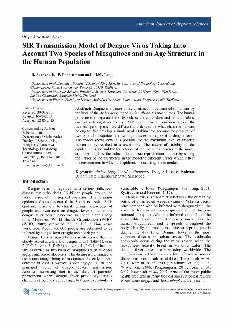
in Fig. 7. Case C, in children, when ε ≠ 0 as shown in Fig. 8.
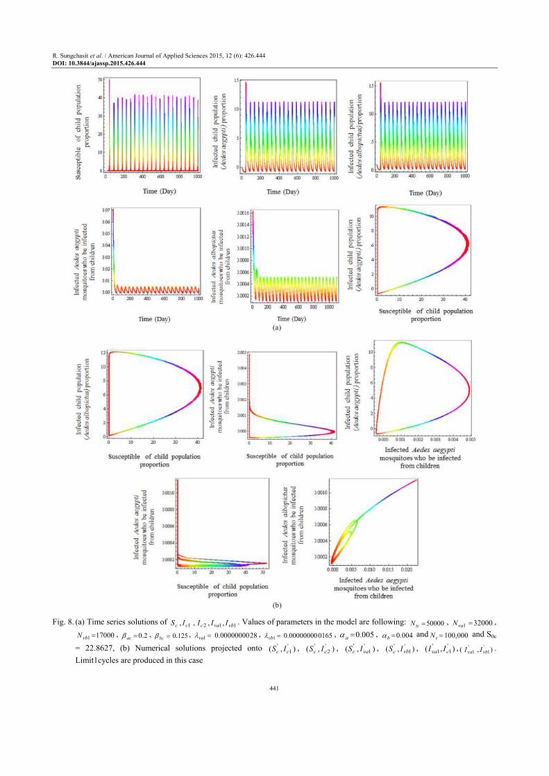
Case D, in adult, when ε ≠ 0 as shown in Fig. 9.
R. Sungchasit et al. / American Journal of Applied Sciences 2015, 12 (6): 426.444
DOI: 10.3844/ajassp.2015.426.444
441
(a)
(b) Fig. 8. (a) Time series solutions of
1121 ,,,, vbvaccc IIIIS . Values of parameters in the model are following: 50000=tcN , 320001 =vaN ,
170001 =vbN , 2.0=acβ , 125.0=bcβ , 280.00000000 1 =vaλ , 01650.00000000 1 =vbλ , 005.0=aα , 004.0=bα and 000,100=tN and S0c
= 22.8627, (b) Numerical solutions projected onto ),('1
'cc IS , ),(
'2
'cc IS , ),(
'1
'vac IS , ),( '
1'
vbc IS , ),( '1
'1 cva II , ),( '
1'
1 vbva II .
Limit1cycles are produced in this case
R. Sungchasit et al. / American Journal of Applied Sciences 2015, 12 (6): 426.444
DOI: 10.3844/ajassp.2015.426.444
442
(a)
(b)
Fig. 9. (a) Time series solutions of
2221 ,,,, vbvaaaa IIIIS . Values of parameters in the model are following: 50000=taN ,
340002 =vaN , 300002 =vbN , 25.0=aaβ , 1428.0=baβ , 750.00000000 2 =vaλ , 06250.000000002 =vbλ , 02.0=aα , 07.0=bα and
000,100=tN , when S0a = 9.26764. (b) Numerical solutions projected onto ),( '2
'aa IS , ),(
'2
'vba IS , ),(
'2
'2 avb II . The solutions
oscillate to the endemic equilibrium state ),,,,( *2
*2
*2
*1
*vbvaaaa IIIIS are limit cycles
Discussion
Several investigations have been conducted using
the SIR and SI models. The SIR and SI models which
provide suitable for the states of children and adult in
two species are used in this study. (Aedes aegypti and
Aedes albopictus).
The basic reproductive number of equations (4a)-(4j)
is defined as follows (Chong et al., 2013):
1 1 1
1 1 1 2
2 ( )
(2( ( ) )
a
b
vb b bc vb c d v vb
va ac va tc vb d c d v
N
N N
α β λ κ µ µ ρ
β λ λ µ κ µ µ
+
+ + +
10
1 1 1
1 1 2
1
2 2 1
2 2 2 2
(2 ) 2 ( ))max { ,
(2 ( ) (2
(2 )) 2 ( ( )
( ( ) )))
2 ( )
(2( ( )
a
b
a
a va tc vb d a va
vb c d v d vb bc
b vb va ac va a c d
v va tc vb d a va a va vb
vb b ba vb a d v vb
va aa va ta vb d a d v
NS
N
N
N
N
N N
α ρ λ µ α ρλ κ µ µ µ β
α ρ β λ α κ µ
µ ρ λ µ α ρ α ρ ρ
α β λ κ µ µ ρ
β λ λ µ κ µ µ
+ + +=
+ +
+ + +
+ + +
+
+ + +
2
2 1 2
2 2 2
2
)
(2 ) 2 ( ))}
(2 ( ) (2 (2 ))
2 ( ( )
( ( ) )))
b
a
b
a va ta vb d a va
vb a d v d vb ba b vb
va aa va a a d v va
ta vb d a va a va vb
N
N
N
N
α ρ λ µ α ρλ κ µ µ µ β α ρ
β λ α κ µ µ ρ
λ µ α ρ α ρ ρ
+ + ++ + +
+ +
+ + +

R. Sungchasit et al. / American Journal of Applied Sciences 2015, 12 (6): 426.444
DOI: 10.3844/ajassp.2015.426.444
443
Table 3. Determination of the values S0 of infected mosquitoes
Iva1 value Ivb1 value Iva2 value Iva2 value S0 value
2.3860×10⁻¹⁸ 6.44744×10⁻⁷ 0.00310
2.5687×10⁻²⁶ 0.000065 - - 0.00732
0 0.00036 - - 0.06795
- - 4.9155×10⁻²³ 0.0007175 0.68842
- - 7.3376×10⁻¹⁴ 1.07169×10⁻⁸ 3.61291
8.234×10⁻⁶ 7.982×10⁻¹⁷ - - 38.6066
3.16331×10⁻⁵ 1.118×10⁻⁶ - - 80.3505
- - 9.933×10⁻⁸ 2.822×10⁻¹⁷ 89.3077
S0 describes the number of infectious human
produced from primary infection of children and
adult. Using the initial values and parameter values
from data, the obtained result of threshold parameter
value S0 for S0c and S0a can be rewritten in
mathematical form as follows:
1 1 1
1 1 1 2
1
0
1 1 1
1 1 2
1
2 ( )
(2( ( )
)(2 ) 2 ( ))in
(2 ( ) (2
(2 )) 2 ( ( )
( ( ) )))
a
b
a
b
vb b bc vb c d v vb
va ac va tc vb d c d
v a va tc vb d a va
c
vb c d v d vb bc
b vb va ac va a c d
v va tc vb d a va a va vb
N
N N
NS
N
N
N
α β λ κ µ µ ρ
β λ λ µ κ µ
µ α ρ λ µ α ρλ κ µ µ µ β
α ρ β λ α κ µ
µ ρ λ µ α ρ α ρ ρ
+
+ + +
+ + +=
+ +
+ + +
+ + +
children
2 2 1
2 2 2 2
20
2 1 2
2 2 2
2
2 ( )
(2( ( ) )
(2 ) 2 ( ))in
(2 ( ) (2
(2 )) 2 ( ( )
( ( ) )))
a
b
a
b
vb b ba vb a d v vb
va aa va ta vb d a d v
a va ta vb d a vaa
vb a d v d vb ba
b vb va aa va a a d
v va ta vb d a va a va vb
N
N N
NS
N
N
N
α β λ κ µ µ ρ
β λ λ µ κ µ µ
α ρ λ µ α ρλ κ µ µ µ β
α ρ β λ α κ µ
µ ρ λ µ α ρ α ρ ρ
+ +
+ +
+ + +=
+ +
+ + +
+ + +
adult
The reproductive rate is depend on the number of
infected mosquitoes Iva1, Ivb1 in children and Iva2, Ivb2
in adult.
From the above table (Table 3), we will see that if the
number of infected mosquitoes is increased, the basic
reproductive rate is also increased.
Moreover, we consider the effect of sinusoidal
variation (ε), we will see that if ε = 0, then the
solutions oscillation to the steady state. The limit
cycle occurs for ε ≠ 0. Thus the limit cycles occurs
while there is the seasonal variation of mosquitoes
(Aedes aegypti and Aedes albopictus). It can be seen
that the dynamical behavior of the endemic state
change while there is the influence of season.
Conclusion
The basic reproductive number of disease is defined by
0 0S S=ɶ . This value is the threshold condition for the
existence of the endemic state. When S0 ≤ 1, the solutions
oscillate to disease free equilibrium state, whereas S0 >
1, the solutions oscillate to the endemic state. The
behaviors of the proportion of susceptible, infective
human into two classes (a child class and an adult
class) and infective vectors of the two species (Aedes
aegypti and Aedes albopictus) are initially positive. If
this can be seen as follow; the infective human are
introduced into the susceptible is bitten during each
period, by the fraction 1
( )
h
h v
bN
N m µ
+ (that the biting
rate b of mosquitoes is the average number of bites per
mosquito per day, µv is the per capita mortality rate of
mosquito, of these bites becomes new infective in the
human population) (Esteva and Vargas, 1998). The
parameters βac, βbc, βaa, βba, βac, λva1, λva2, λvb1 and
λvb2are effects to the basic reproductive number of this
disease as we see in (6f)-(6h). If the basic reproductive
number is less or equal than one, then the infective
replaces less than one, then disease dies. On the other
hand, if this number is greater than one and when the
susceptible fraction get large enough to birth of new
susceptible, then there are secondary infections and
endemic equilibrium state is occurred. As we can see in
this study, the seasonal parameters such as ε, ρva and
ρvb which are the measure of influence on the
transmission process reflect the environment.
Acknowledgment
This study is supported by King Mongkut’s Institute of Technology Ladkrabang and National Research Council of Thailand.
Author’s Contributions
The work preseted here was carried out in collaboration between all authors. R. Sungchasit, P. Pongsumpun and I.M. Tang. Designed and analyzed the model. All authors have contributed to, seen and approved the manuscript.
Ethics
The authors confirm that this work is original and contains has not published elsewhere.

R. Sungchasit et al. / American Journal of Applied Sciences 2015, 12 (6): 426.444
DOI: 10.3844/ajassp.2015.426.444
444
References
WHO, 2009. Fact sheets: Dengue and dengue
haemorrhagic.
Pongsumpun, P.P. and I. Tang, 2001. A realistic age
structured transmission model for dengue
hemorrhagic fever in Thailand. Math. Comput.
Modell., 32: 336-340.
Syafruddin, S. and M.S.M. Noorani, 2012. SEIR Model
for transmission of dengue fever in selangor
Malaysia. Int. J. Mod. Phys. Conf. Ser., 9: 380-389.
DOI: 10.1142/S2010194512005454 Kerpaninch, A., V. Watanaveeradej, R. Samakosses, S.
Chumnanvanakij and T. Chulyamitporn et al., 2001. Perinatal dengue infection. Southeast Asian J. Trop Med. Publ. Health, 32: 488-493. PMID: 11944704
Kabilan, L., S. Balasubramanian, A.M. Keshava, V. Thenmozhi and C. Sehar et al., 2003. Dengue disease spectrum among infants in the 2001 dengue epidemic on Chennai, Tamil Nadu, India. J. Clin. Microbiol., 41: 3919-3921.
DOI: 10.1128/JCM.41.8.3919-3921.2003
Malhotra, N., C. Chanan and S. Kumar, 2006. Dengue
infection in pregnancy. Int. J. Gynecol. Obstet, 94:
131-132.
Wiwanitkit, V., 2006. Dengue haemorrhagic fever in pregnancy: Appraisal on Thai cases. J. Vector Borne Disease, 43: 203-205.
Pongsumpum, P., 2011. Seasonal transmission model of
dengue virus infection in Thailand. J. Basic Applied
Sci. Res., 1: 1372-1379.
Joshi, V., D.T. Mourya and R.C. Sharma, 2002.
Persistence of dengue -3 virus though transovarial
passage in successive generations of Aedes aegypti
mosquitoes. Am J. Trop Med. Hyg., 67: 158-61.
Koenraadt, C.J.M., J. Aldstadt, U. Kijchalao, A.
Kengluecha and J.W. Jones et al., 2007. Spatial and
temporal patterns in the recovery of Aedes aegypti
(Diptera: Culicidae) populations after insecticide
treatment. J. Med. Entomol., 44: 65-71. DOI:
10.1603/0022-2585(2007)44[65:SATPIT]2.0.CO;2
Hotta, S., 1998. Dengue vector mosquitoes in Japan: The
role of Aedes albopictus and Aedes aegypti in the
1942-1944 dengue epidemics of Japanese Main
Islands [in Japanses with English summary]. Med.
Entomol. Zoollogy, 49: 267-274.
Smith, D.L., K.E. Battle, S.I. Hay, C.M. Barker and
T.W. Scott et al., 2012. Macdonald and a theory for
the dynamics and control mosquito-transmitted
pathogens. PLos Pathog, 8: e1002588-e1002588.
Diekmann, D. and J. Heesterbeek, 2000. Mathematical
Epidemiology of Infectious Disease: Model
Building, Analysis and Interpretation. 1st Edn., John
Wiley and Sons, Chichester, ISBN-10: 0471492418,
pp: 303.
Nuraini, N., E. Soewono and K. Sidarto, 2007.
Mathematical model of dengue disease transmission
with severe dhf compartment. Bullentin Malaysian
Math. Sci., 30: 143-157.
Yaacob, Y., 2007. Analysis of a dengue disease
transmission model with immunity. Matematika,
23: 75-81.
Esteva, L. and C. Vargas, 1998. Analysis of a dengue
disease transmission model. Math. Biosciences, 15:
131-151. DOI: 10.1016/S0025-5564(98)10003-2
Edelstein-Keshet, L., 1988. Mathematical Models in
Biology. 1st Edn., SIAM, Norwood Mass,
ISBN-10: 0898719143, pp: 586.
Chong, N.S., J.M. Tchuenche and R.J. Smith, 2013. A
mathematical model of avian influenza with half-
saturated incidence. J. Theory Biosciences, 133:
23-38. DOI: 10.1007/s12064-013-0183-6


