
September Arctic sea ice minimum predicted by spring
melt pond fractionDanny Feltham and David Schroeder
Centre for Polar Observation and Modelling,Department of Meteorology,
University of Reading, UKThanks to Daniela Flocco, Michel Tsamados
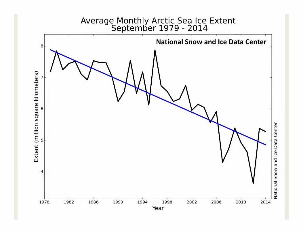
National Snow and Ice Data Center
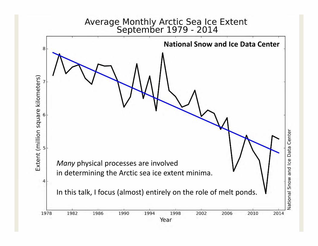
Many physical processes are involvedin determining the Arctic sea ice extent minima.
In this talk, I focus (almost) entirely on the role of melt ponds.
National Snow and Ice Data Center
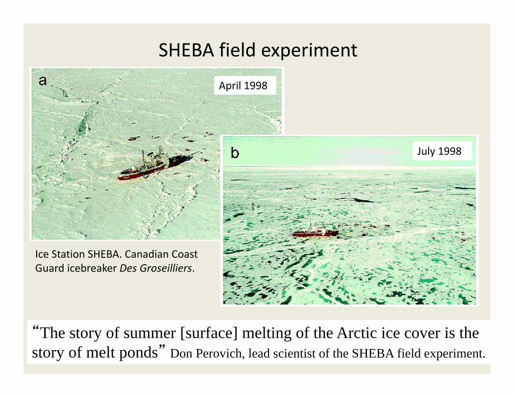
SHEBA field experiment
Ice Station SHEBA. Canadian CoastGuard icebreaker Des Groseilliers.
April 1998
July 1998
“The story of summer [surface] melting of the Arctic ice cover is the story of melt ponds” Don Perovich, lead scientist of the SHEBA field experiment.
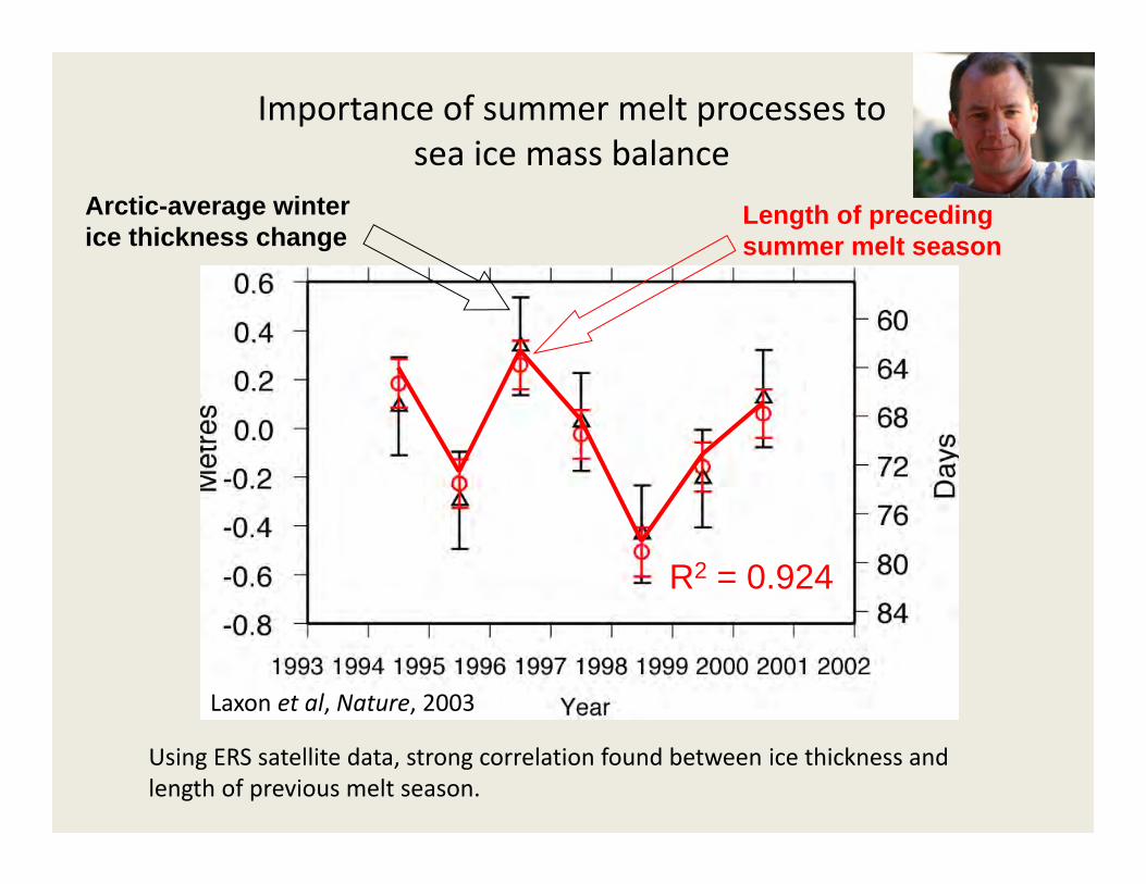
Importance of summer melt processes to sea ice mass balance
Arctic-average winter ice thickness change
Length of preceding summer melt season
R2 = 0.924
Laxon et al, Nature, 2003
Using ERS satellite data, strong correlation found between ice thickness and length of previous melt season.

Melt pondsSHEBA August 14, 1998
• Surface snow and ice melts due to absorbed solar, short wave radiation and accumulates in ponds. Ponds are typically 1-100m wide and 0.1-1.5m deep.
• Pond coverage ranges from 5—50%.
• albedo of pond-covered ice < albedo of bare sea ice or snow covered ice(0.15—0.45) (0.52—0.87)
• Deeper ponds have a lower albedo, which saturates at about 1.5m depth.
• Ponded ice melt rate is 2—3 times greater than bare ice and melt ponds contribute to the albedo feedback mechanism.
• Melt ponds are not (yet) explicitly represented in Global Climate Models.
SHEBA CD, Perovich et al 1999
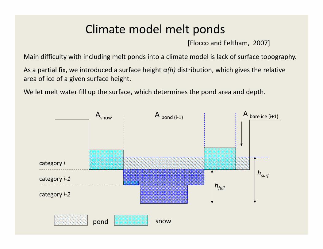
Climate model melt ponds
Main difficulty with including melt ponds into a climate model is lack of surface topography.
As a partial fix, we introduced a surface height α(h) distribution, which gives the relativearea of ice of a given surface height.
We let melt water fill up the surface, which determines the pond area and depth.
[Flocco and Feltham, 2007]
snowpond
Asnow
category i
category i-1
category i-2
A pond (i-1) A bare ice (i+1)
hfull
hsurf

Melt pond parameterisation features• Pond volume collects on ice of lowest height.• Hydrostatic balance is maintained throughout.• Vertical drainage is by Darcy’s law with a variable permeability.
• Melt water is lost during ridging.• Melt water is transported as a tracer on each thickness class.• During refreezing, a pond lid forms that grows/melts at each time
step.
“trapped” melt pond
ice lid growing downwards
Our melt pond model has now been incorporated into a climate sea ice model (CICE) and is being included in climate models.
POSTER: Refreezing of melt ponds[Flocco, Feltham, et al]
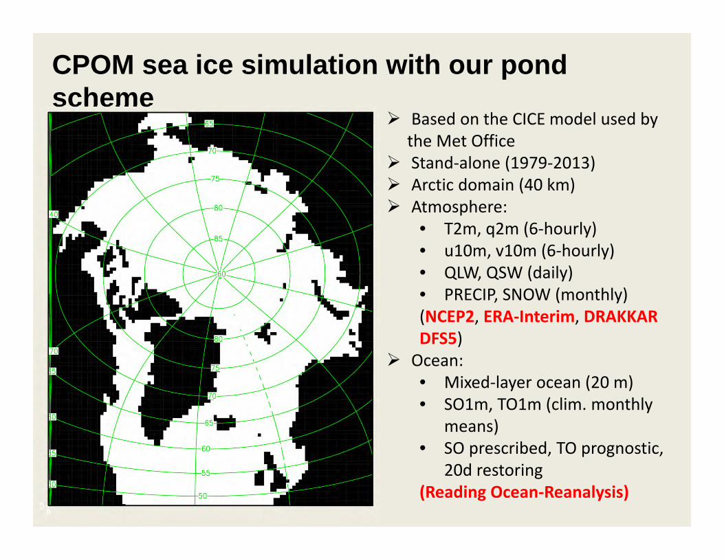
CPOM sea ice simulation with our pond scheme
Based on the CICE model used by the Met Office
Stand-alone (1979-2013) Arctic domain (40 km) Atmosphere:
• T2m, q2m (6-hourly)• u10m, v10m (6-hourly)• QLW, QSW (daily)• PRECIP, SNOW (monthly)(NCEP2, ERA-Interim, DRAKKAR DFS5)
Ocean:• Mixed-layer ocean (20 m)• SO1m, TO1m (clim. monthly
means)• SO prescribed, TO prognostic,
20d restoring(Reading Ocean-Reanalysis)
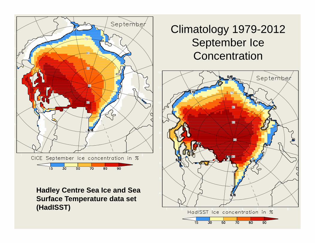
Climatology 1979-2012September Ice Concentration
Hadley Centre Sea Ice and Sea Surface Temperature data set (HadISST)
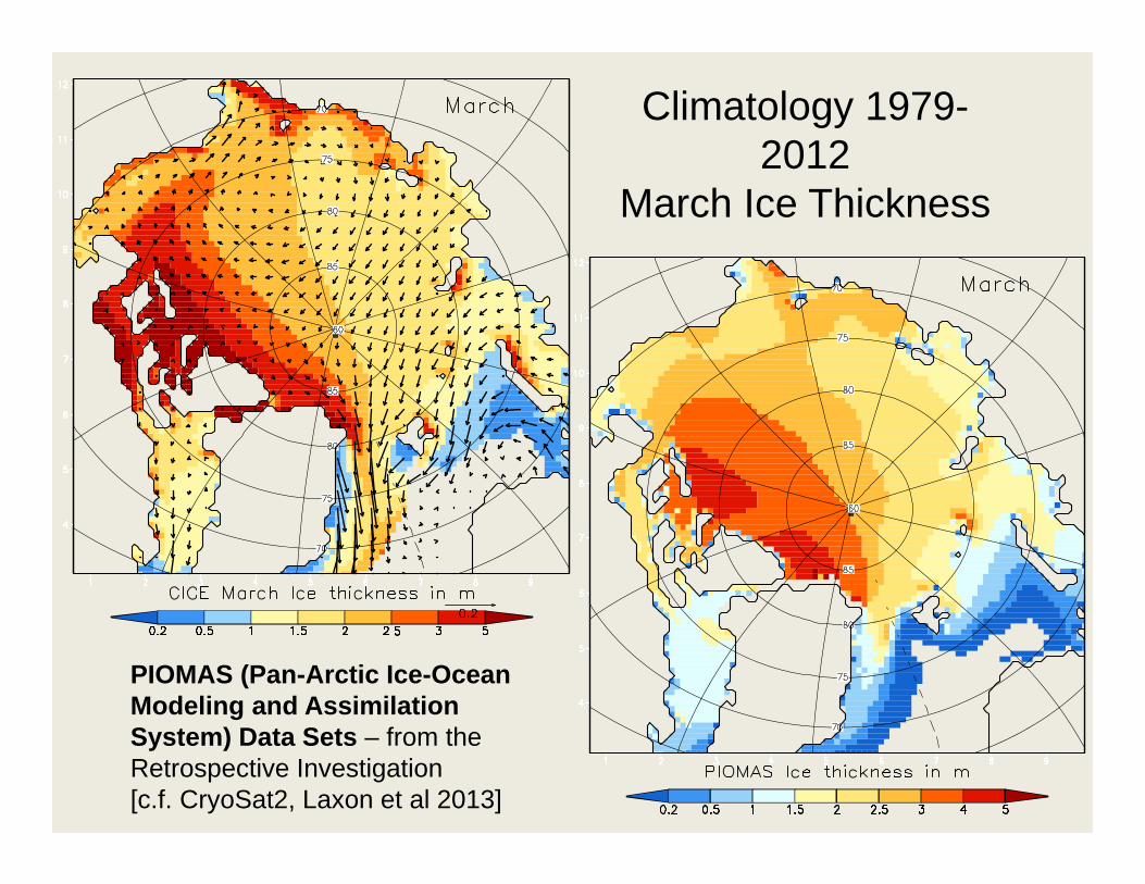
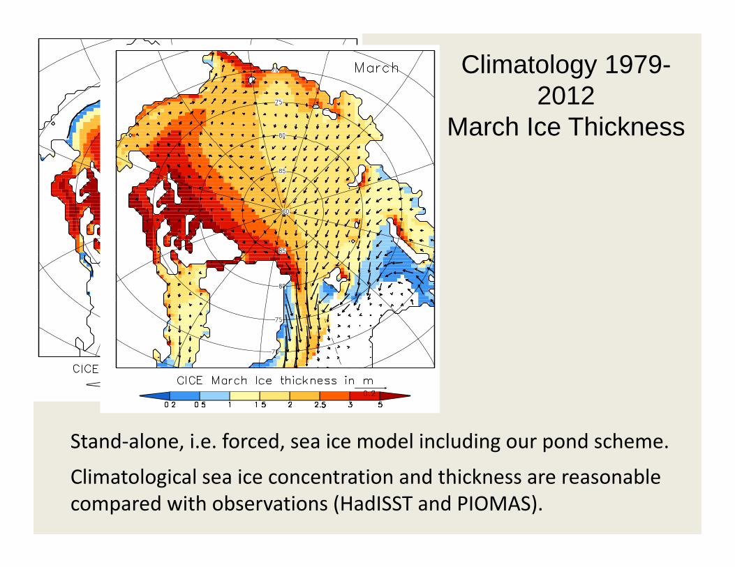
Climatology 1979-2012
March Ice Thickness
PIOMAS (Pan-Arctic Ice-Ocean Modeling and Assimilation System) Data Sets – from the Retrospective Investigation[c.f. CryoSat2, Laxon et al 2013]
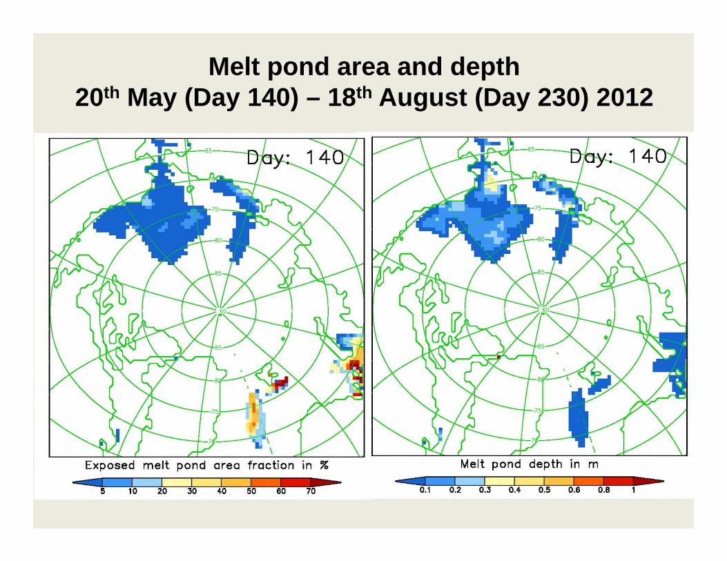
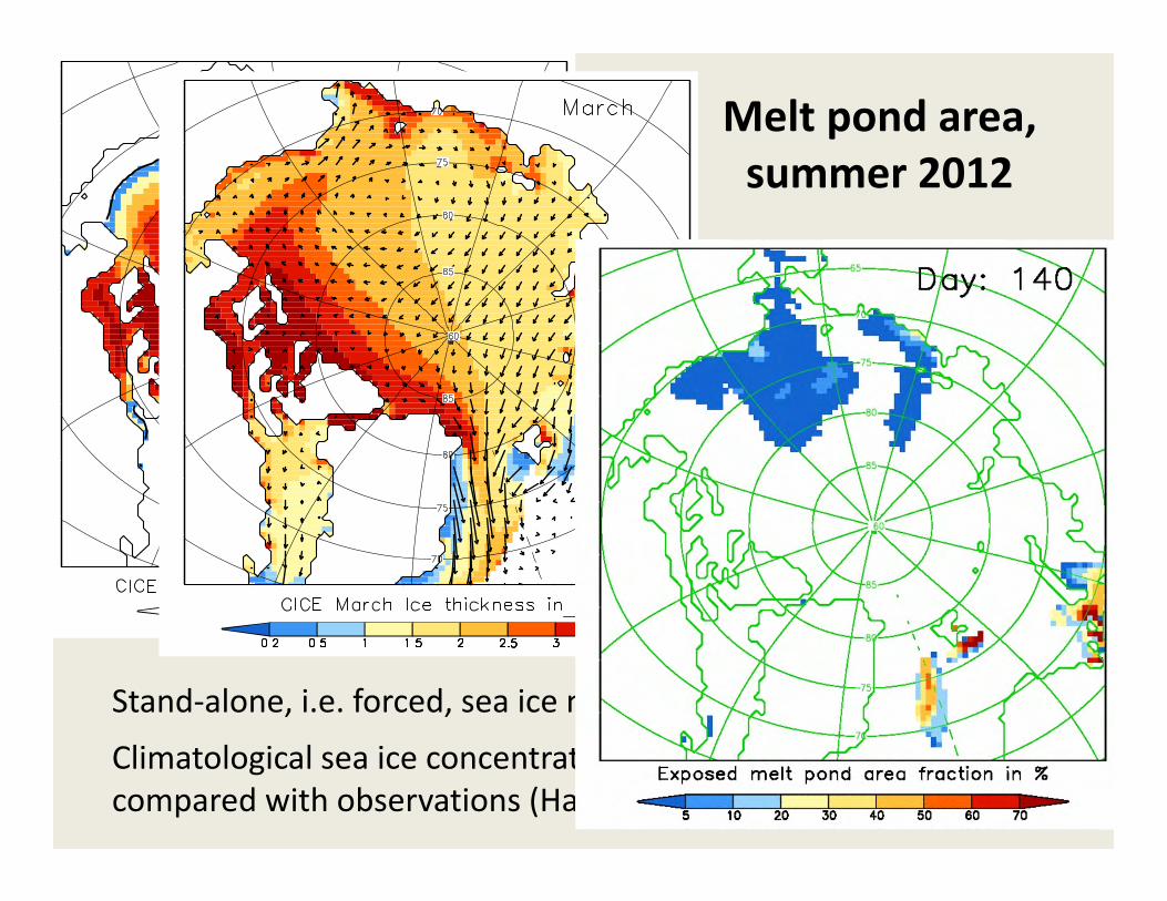
Melt pond area and depth20th May (Day 140) – 18th August (Day 230) 2012
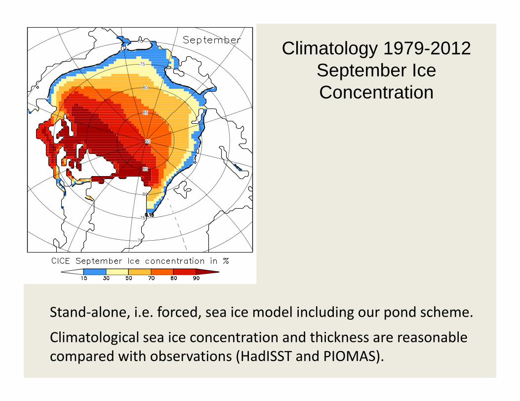
Climatology 1979-2012September Ice Concentration
Stand-alone, i.e. forced, sea ice model including our pond scheme.
Climatological sea ice concentration and thickness are reasonable compared with observations (HadISST and PIOMAS).
Climatology 1979-2012
March Ice Thickness
Stand-alone, i.e. forced, sea ice model including our pond scheme.
Climatological sea ice concentration and thickness are reasonable compared with observations (HadISST and PIOMAS).
Stand-alone, i.e. forced, sea ice model including our pond scheme.
Climatological sea ice concentration and thickness are reasonable compared with observations (HadISST and PIOMAS).
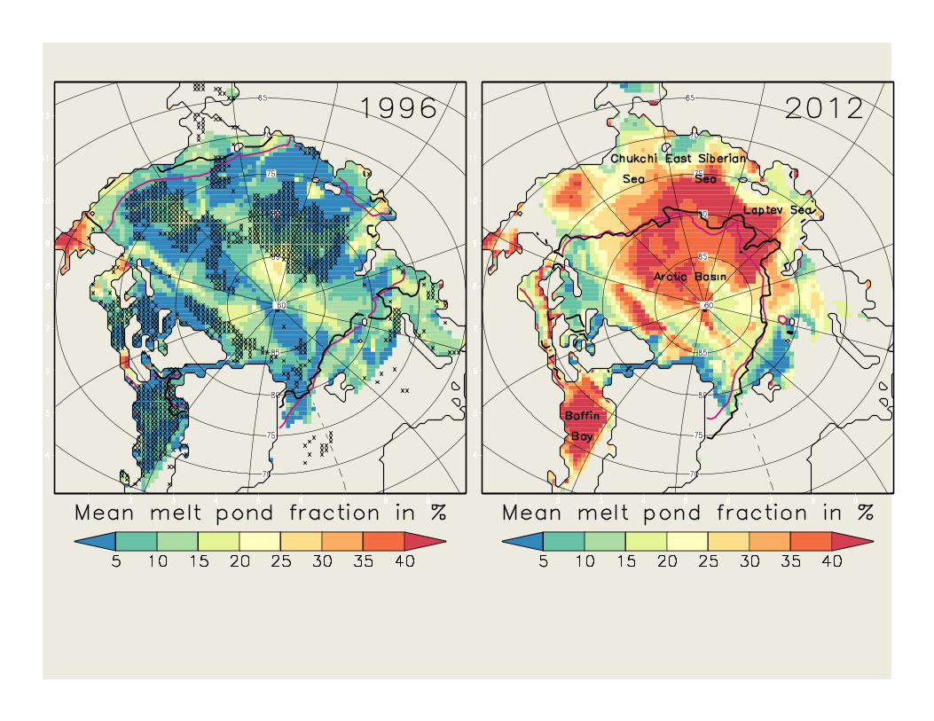
Melt pond area, summer 2012

1996
2012
1980s
1990s
2000s
Seasonal evolution of melt ponds
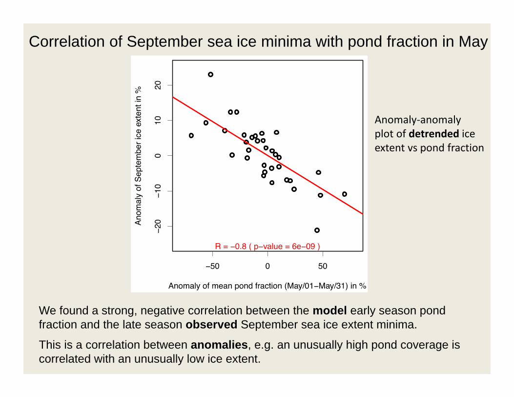
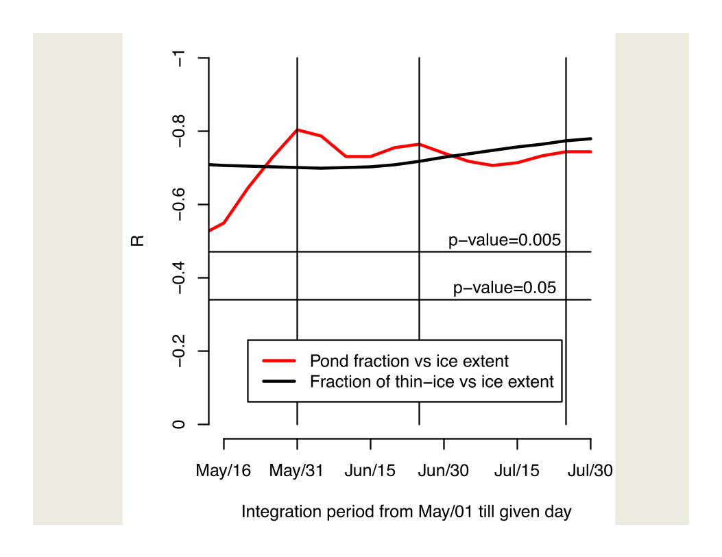
We found a strong, negative correlation between the model early season pond fraction and the late season observed September sea ice extent minima.
This is a correlation between anomalies, e.g. an unusually high pond coverage is correlated with an unusually low ice extent.
Correlation of September sea ice minima with pond fraction in May
Anomaly-anomaly plot of detrended iceextent vs pond fraction
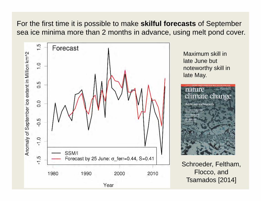
For the first time it is possible to make skilful forecasts of September sea ice minima more than 2 months in advance, using melt pond cover.
Maximum skill inlate June but noteworthy skill in late May.
Schroeder, Feltham, Flocco, and
Tsamados [2014]
1980 1990 2000 2010
45
67
8
Year
Sep
tem
ber i
ce e
xten
t in
Mill
ion
km^2
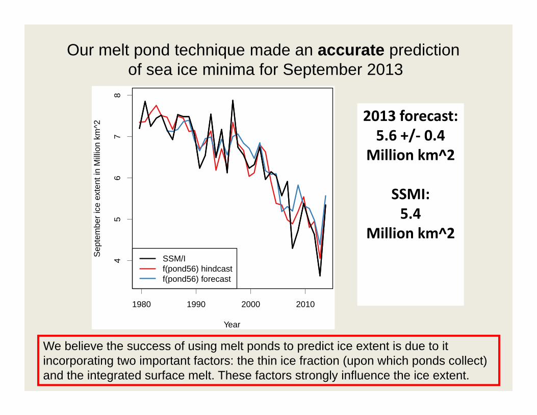
SSM/If(pond56) hindcastf(pond56) forecast
2013 forecast: 5.6 +/- 0.4
Million km^2
SSMI:5.4
Million km^2
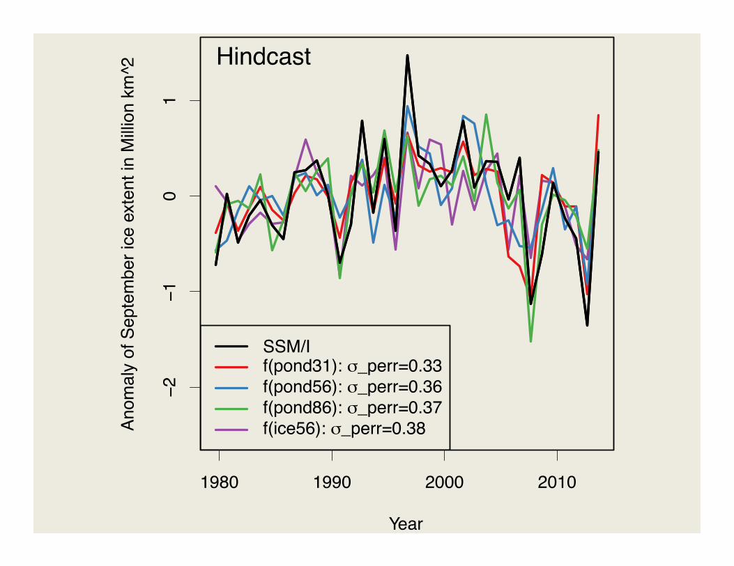
Our melt pond technique made an accurate prediction of sea ice minima for September 2013
We believe the success of using melt ponds to predict ice extent is due to it incorporating two important factors: the thin ice fraction (upon which ponds collect) and the integrated surface melt. These factors strongly influence the ice extent.
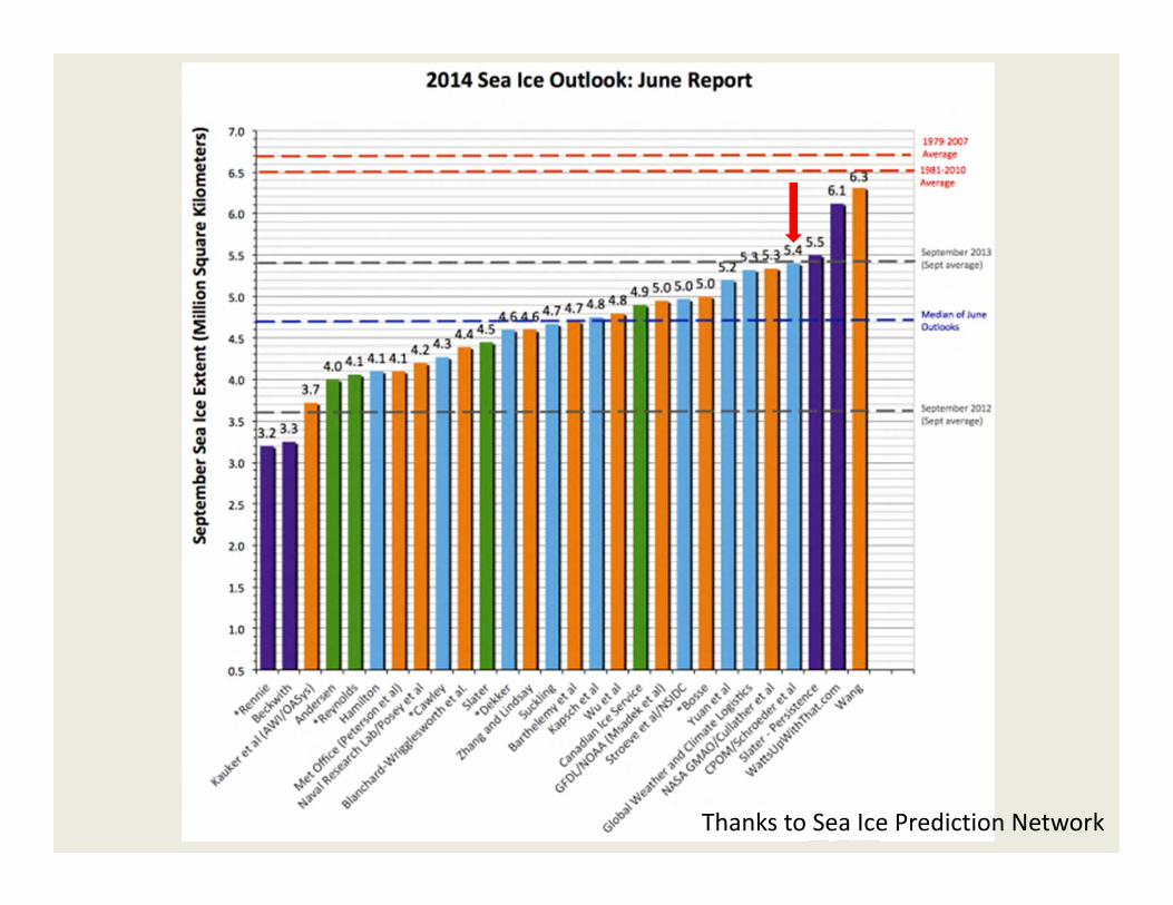
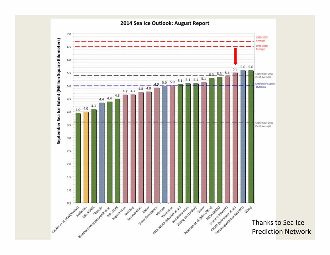
Thanks to Sea Ice Prediction Network
Thanks to Sea IcePrediction Network
Concluding remarks• On 16 June, we predicted the 2014 sea ice minimum to be
5.4 M km2 +/- 0.5 M km2. The actual value was 5.28 M km2. So... pretty good! But we were also lucky.
Concluding remarks• On 16 June, we predicted the 2014 sea ice minimum to be
5.4 M km2 +/- 0.5 M km2. The actual value was 5.28 M km2. So... pretty good! But we were also lucky.
• Strong correlation found between pond fraction in spring and September sea ice (R=-0.80 for de-trended time-series), physically explained by the albedo feedback mechanism.
• We can forecast September ice extent with an error of about 0.44 M km2 and a skill value of S = 0.41.
• A physically realistic melt pond model has been incorporated into a climate sea ice model.
• Including physically-realistic melt ponds promises to improve GCMs for seasonal sea ice forecasts and climate predictions.
Questions?

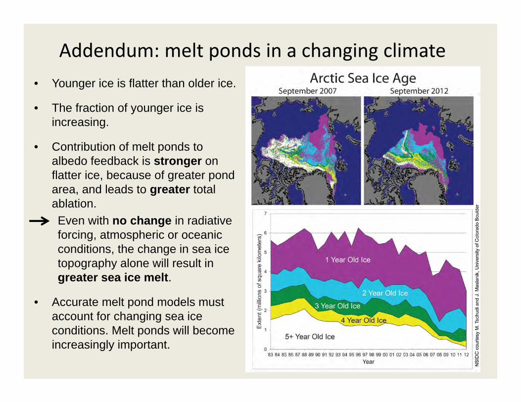
• Younger ice is flatter than older ice.
• The fraction of younger ice is increasing.
• Contribution of melt ponds to albedo feedback is stronger on flatter ice, because of greater pond area, and leads to greater total ablation.Even with no change in radiativeforcing, atmospheric or oceanic conditions, the change in sea ice topography alone will result in greater sea ice melt.
• Accurate melt pond models must account for changing sea ice conditions. Melt ponds will become increasingly important.
Addendum: melt ponds in a changing climate
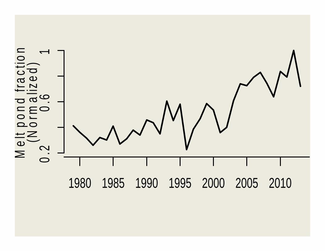
Mel
t pon
d fra
ctio
n
1980 1985 1990 1995 2000 2005 2010
0.2
0.6
1(N
orm
aliz
ed)
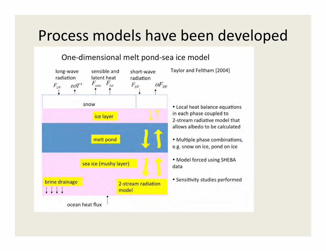
Process models have been developed
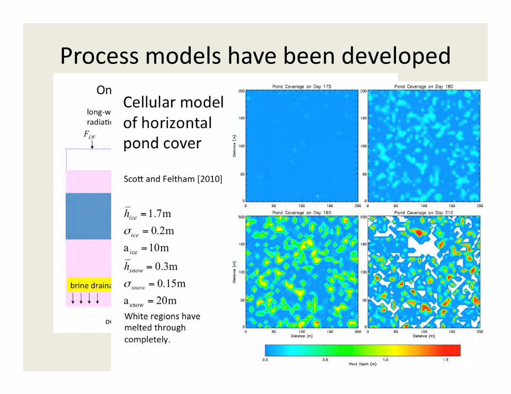
Process models have been developed
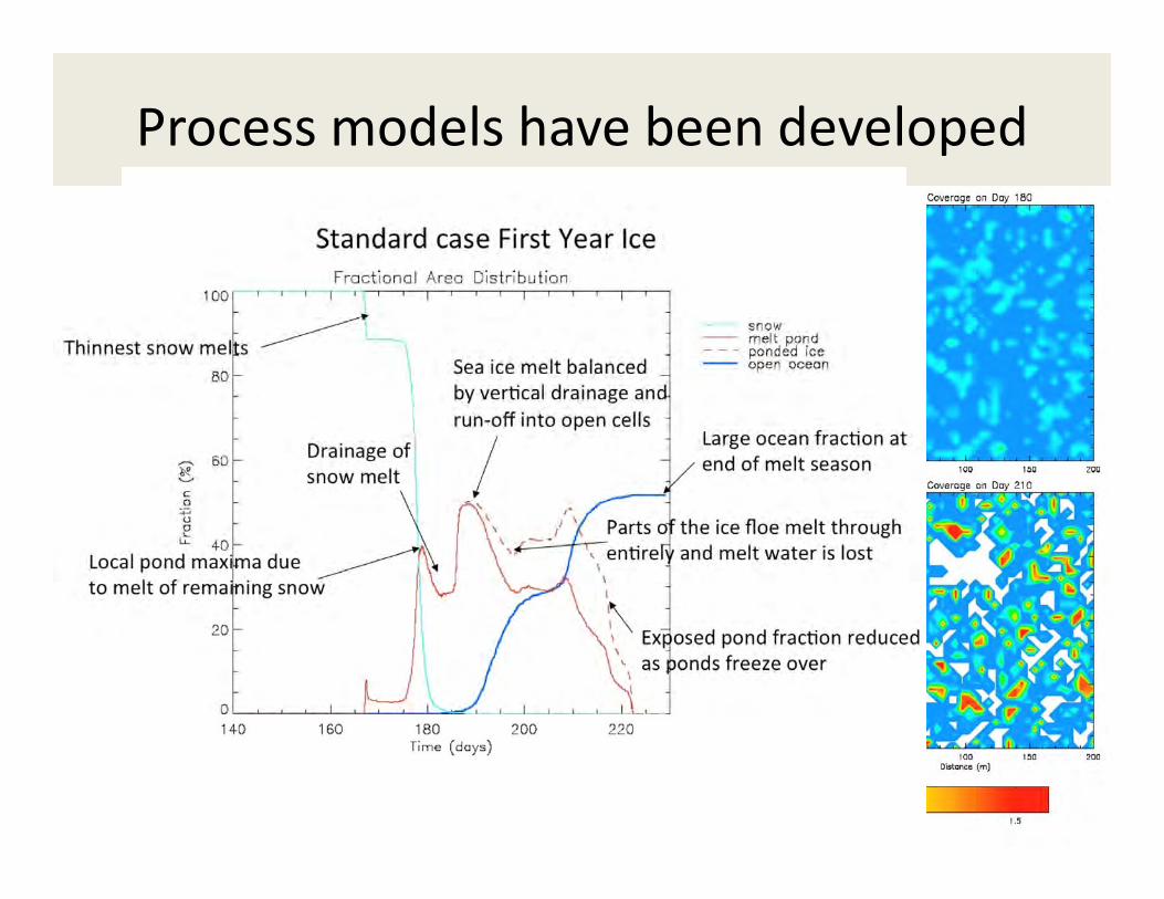
Process models have been developed
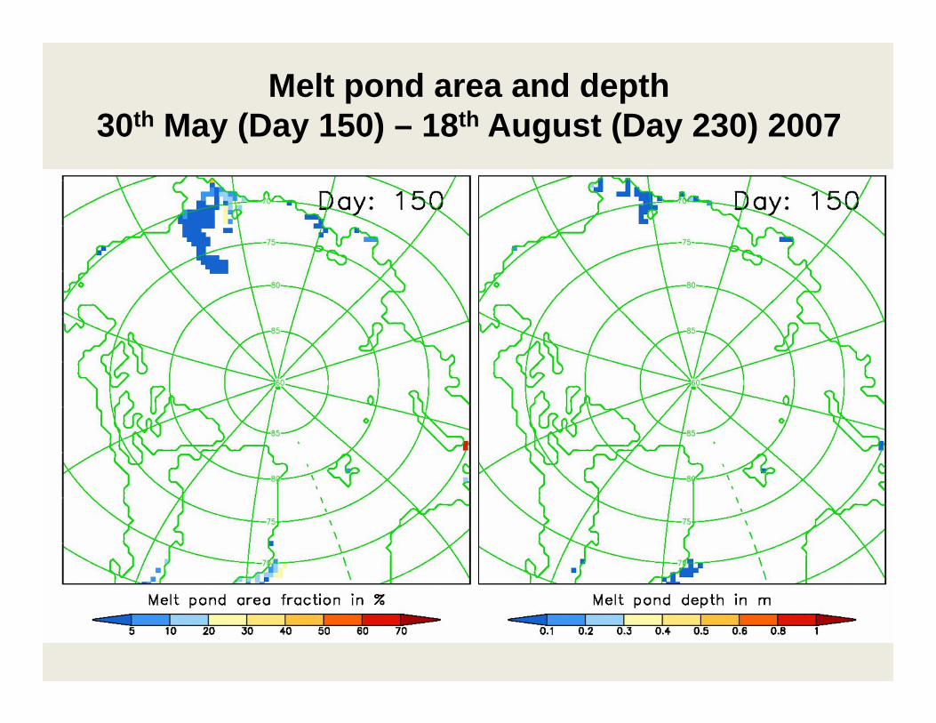
Melt pond area and depth30th May (Day 150) – 18th August (Day 230) 2007


