
1
Leesversie proefschrift
Sensorische en Instrumentele Analyse van
Voedselgeuren
Johannes Hendrikus Fransiscus Bult

2
1 General introduction
According to popular belief, one of the world’s best-kept secrets is the Coca-Cola recipe. In
spite of the secrecy surrounding this recipe, detailed ingredient lists and preparation descriptions
are available, allegedly derived from a retrieved notebook of J.S. Pemberton (the founder of the
company) and statements by a Russian co-worker that defected the company (Pendergrast,
2000). Besides a number of non-aromatic ingredients like water, sugar, citric acid, caffeine,
fluid-extracted alkaloids from cola leaves and carbon dioxide, the available recipes list a number
of aromatic ingredients: Vanilla, lime juice, caramel and essential oils from orange, lemon,
nutmeg, cinnamon, coriander, and neroli. Other sources also mention the addition of essential
oils from lavender and cassia (Pendergrast, 2000). Each of these aromatic ingredients contributes
tens up to hundreds of different volatile components to the drink, each of which is a potential
odorant. Hence, a very complex mixture of odorants produces one of the worlds most known
aromas, holistically perceived as cola.
To understand how an aroma percept is formed, it is likely to be important to know which
chemical substances contribute to the aroma mixture, and how these individual substances are
perceived (a decompositional approach). The present thesis deals with an analytical technique
that combines the instrumental pre-treatment of food-born odorants with their subsequent
chemical, analytical and sensory detection: gas chromatography olfactometry (GCO). This
method unifies two scientific traditions in which very distinct methodological languages are
spoken. The chemical analytical tradition excels in the nearly deterministic assessment of
odorant quantities, only satisfied with instruments that show test-retest reliabilities
approximating 100%. The perceptual psychological tradition, on the other hand, accepts
probabilistic models of human behaviour as their daily practice, and is hardly surprised by the

3
fact that a human observer practically never generates identical responses to identical odorant
concentrations.
In the eyes of a flavour chemist, GCO panellists are unreliable instruments. There is no better
alternative available yet, so until that day flavour chemists will continue to use man as a method
to study matter. However, psychological knowledge may help to improve the reliability of the
human instrument. This is discussed in the first section of the thesis. In contrast, GCO
experiments are interesting natural experiments in the eyes of a perceptual psychologist. Here,
the perceptual system is subjected to a number of conditions similar to those known from
scientific experiments on human perception. Much about perceptual mechanisms is known and,
hence, much of the variability of GCO panellists’ responses may be understood by the perceptual
psychologist. However, the GCO practice has led to a number of assumptions regarding human
perception that were not studied thus far. In that respect, for the perceptual psychologist, the
experimental practices used in GCO provide an interesting approach to study man. This will be
discussed in the second section of the thesis.
I - Man as a method to study matter
Gas chromatography
Chromatography is a method used to decompose complex mixtures of chemicals into their
constituents. In essence, the method entails the forced transfer of chemical components along an
adsorptive or dissolvent material, which usually is packed in a column or which constitutes the
inner lining of a column. The affinity for the adsorbent differs over chemicals and their retention
times on the column differ accordingly. Hence, chemicals that are forced through the column
simultaneously will elude separately.

4
The principle of separating chemicals due to their differing affinities to an adsorbent dates
back to the work of chemists like Schönbein and Goppelsröder (Beneke, 1999). In the 1860s they
used filter paper to separate chemicals contained in liquids that were absorbed in the paper
through the capillary effect. Later, it was the Russian botanist Mikhail Tswett who, driven by the
motive to characterize and separate the chemicals that contributed to the colour of leaves, used
various solvents to extract ‘colour’ from fresh and dried leaves (Tswett, 1906b; Tswett, 1906a).
He then separated these pigments by having them adsorbed differentially to precipitated calcium
carbonate, inulin or powdered sucrose. Subsequently, Tswett characterised these components
chemically by measuring their spectral absorption patterns. In the words of Tswett, “the
components of a pigment mixture separate on a column like the light rays of a spectrum –
allowing for both a qualitative and a quantitative analysis”. Hence, the separation process was
coined the “chromatographic method” and the resulting quantitative absorption patterns of the
mixture components a “chromatogram”. This procedure – the extraction of the chemicals, their
separation on an adsorbent material and their consecutive quantification and characterisation – is
still at the core of modern-day chromatography. Tswett presented his work for the first time at a
St. Petersburg convention in 1901 and presented it as the chromatographic method in 1906
(Tswett, 1906b; Tswett, 1906a). Tswett, who worked under unfavourable conditions with
solvents like CS2 (his favourite), petroleum ether, benzene, xylene, toluene, various alcohols,
chloroform, acetone and acetaldehyde, died from a chronic throat inflammation in 1919 at the
age of 47. Possibly due to the turbulent period that Russia went through in the early 20th century
and its political and social isolation, Tswett’s work went into oblivion until nearly three decades
after its first presentation in 1901.
Although the technique of the adsorption of chemicals to solids by Tswett enabled the
separation of chemicals dissolved in liquids in spatial terms, a revolutionary new
conceptualisation of chromatography by Martin and Synge (Martin and Synge, 1941) allowed the

5
improved separation of a greater variety of dissolved chemicals in temporal-spatial terms. Their
method of ‘partitioning chromatography’ employed a column containing counter-current liquids
between which dissolved chemicals partitioned. Due to differences in partitioning behaviour, the
chemicals separated spatially and could be captured at the end of the column, due to their
separation in time. This fundamental improvement allowed for the thorough study of complex
mixtures of chemicals. It won the authors a Nobel Prize in 1952. In the 1941 publication that
introduced liquid-liquid chromatography, Martin and Synge discussed the possibilities of gas-
liquid chromatography according to the same working principle of partitioning. Indeed, gas-
liquid chromatography was realised in the early 1950s (James and Martin, 1952). Its principle -
the separation of gaseous chemicals by forcing them through a capillary column lined with a
liquid phase that retains the gaseous components at different rates - is still used to decompose
mixtures of gaseous chemicals, including aromas. We will further refer to this technique as gas
chromatography.
Gas chromatography olfactometry (GCO)
When odorous chemicals elude from a capillary column, their presence may be detected by
instruments like flame ionisation detectors (FID) or by mass spectrometry (MS). Although this
allows for a reliable quantification of the chemicals, the found quantities are poor estimates of
the intensity of the odour sensations that these chemicals invoke. Due to large differences in
detection thresholds between odorants, the capacity of chemicals to invoke odour sensations at a
given concentration level varies strongly. Hence, relative quantities of the components in the
mixture are poor indicators of their relative contributions to the mixture’s aroma. A better
estimate of each component’s contribution to the aroma may be obtained by sensory evaluation
of the separated constituents. Thus, by replacing the FID with a sufficiently large panel of
subjects that sniff the effluents of the gas chromatograph in an effort to detect and characterize

6
the odour-active chemicals, a new method called gas chromatography olfactometry (GCO) was
introduced (Fuller et al., 1964; Dravnieks and O'Donnell, 1971).
Figure 1.1 shows a schematic overview of a GCO session. The physical detection and
identification of volatile components by FID/MS is combined with the responses of panellists to
perceived odours on one unifying time scale. Because human subjects are inconsistent
responders – they do not always detect the same odorants under the same conditions – sessions
need to be repeated between- or within-subjects to obtain acceptable reliabilities of detection
scores. Therefore, responses over a number of identical GC sessions need to be aggregated
before odour impacts may be assessed. The requirement of session repetition poses a threat to the
reliability of odour impact assessment in lengthy GCO experiments. GC column characteristics
may change due to repeated usage and variations in carrier gas pressure and in oven temperature
may occur. As a consequence, retention times of odorants may vary, due to which timed
responses to odorants by panellists may not co-occur in time. Because a number of GCO
methods quantify the impact of odorants by employing the co-occurrence of responses, a low
reliability of retention times will reduce odour impact measures. To prevent this, panellists’
Figure 1.1. Schematic representation of a GCO session. Volatile components (represented by coloured circles) are injected simultaneously at time T0 through an injector (Inj.) into a capillary which is gradually heated up in an oven. Being forced through the capillary, the volatile components separate spatially and are released separately in time (T1, T2, T3 etc.) from the capillary and simultaneously detected by FID (top graph) and a human subject at the sniffing port (SP). In this example, subjects pushed a button whenever an odour was perceived at the SP (bottom graph).
t (min)
0 5 10 15 20 25
Res
pons
e
T0
T1
T2
T3
Inj.
Capillary
SP
Oven
FID
T2

7
response times may be corrected according to the retention times of known components in the
evaluated mixture. This may be done by linear interpolation of response times in relation to
normalised elution times, which should raise the signal to noise ratio of combined panel
responses. This issue will be discussed in chapter 2 of this thesis.
Assessing odour impact in GCO experiments
To quantify the sensory impact of the effluents, several sensory methods are in use. These
methods fall into three categories:
1. Flavour Dilution (FD) methods use the number of times a sample needs to be diluted
until it is detected by less than 50% of the panellists as a measure of odour impact.
Examples of this approach are CHARM Analysis (Acree et al., 1984) and Aroma Extract
Dilution Analysis (Ullrich and Grosch, 1987).
2. Detection Frequency (DF) methods employ the number of coinciding panel detection
responses to a stimulus as an indicator of its odour impact (Van Ruth and Roozen, 1994;
Pollien et al., 1997; Pollien et al., 1997). The more panellists respond simultaneously to
an odorant, the higher the estimated odour impact. This method is also referred to as
Olfactory Global Analysis (Le Guen et al., 2000; Grosch, 2001).
3. Intensity rating methods like the Osme method (Da Silva et al., 1994; McDaniel et al.,
1990) use panellists’ intensity ratings of undiluted GC effluents to assess their odour
impact. The higher the intensity ratings the higher the odour impact.
The three methods generate highly comparable results when used to determine the main
contributors to an aroma (Van Ruth and O'Connor, 2001; Le Guen et al., 2000). However, a
number of fundamental shortcomings have been noted regarding their use and the interpretation
of their results.

8
First of all, FD and DF methods falsely assume that the perceived odour impact relates
linearly to odour threshold concentrations. In the case of FD methods, odour impact is
conceptualised as the number of dilution steps needed for a panellist to reach detection threshold
(the odour activity value or OAV). A common critique of this approach is that perceived
intensity is not a linear function of the OAV (Frijters, 1978; Abbott et al., 1993). Instead, odour
intensity tends to approximate a power function of odorant concentration (Mitchell, 1971;
Stevens, 1975) with threshold levels at a wide range of odorant concentration values. On their
turn, detection frequency methods assume implicitly that detection thresholds differ between
panellists. Panellists that respond to an odorant have thresholds below the presented
concentration so that the number of responding panellists reflects the generally perceived
intensities. Although detection probabilities may relate to odorant intensity/impact, the often
Gaussian or even multimodal (more than one modus) sensitivity distributions in populations
(Pollien et al., 1997) allow, at best, ordinal models describing this relation.
Second, FD and intensity rating methods lack reliability estimates for odour detection. GCO
sessions consist of vigilance tasks in which subjects are asked to detect and respond to
unannounced signals. Often, the only indications for the presence of odours are the panellist
reports, because very-low threshold concentrations rarely lead to FID responses. Therefore, the
flavour chemist wonders whether he or she can reliably conclude that the panel perceived an
odorant at a certain retention time or not. In this respect, it is generally assumed that FD and
intensity rating measures are more informative than mere odour detections (DF), since the former
consist of a variety of dilutions steps (FD) or responses on nearly continuous response scales
(intensity ratings), whereas that latter (DF) provides dichotomous results. As a consequence,
fewer subjects (and repetitions) are employed in dilution- and, especially, intensity studies
compared to DF studies (Table 1.1). However, in spite of this general assumption, in the current

9
practice of FD and intensity rating procedures, the reliability of the answer to whether an odour
was detected or not remains unsure.
First, odour impact assessment methodologies all share the problem that they need to define
cut-off scores: How many panellists should respond simultaneously to ascertain that an odour
was perceived? In FD methodology that number is 50% and in DF methodology it is the
percentage of panellists that responded simultaneously in a blank session. However, from
vigilance studies (Vickers et al., 1977; Swets, 1977; Warm et al., 1991) it is known that
panellists adjust their decision criterion depending on the perceived stimulus probability: the
number of responses will decrease when perceived stimulus probabilities decrease and the
number will increase when perceived stimulus probabilities increase (Williges, 1969; Colquhoun
and Baddeley, 1967). Hence, cut-off scores suffer from the occurrence of systematic errors.
In addition, cut-off scores are generally estimated on the basis of one average. This practice
does not allow for the estimation of cut-off score reliability intervals. Therefore, cut-off scores
are also subject to random errors of unknown proportions.

10
In the case of intensity ratings, higher-than-zero intensity ratings suggest odour detection.
However, because false detections will also be accompanied by non-zero intensity ratings, the
above question translates to: “At which intensity level can I reliably state that the panel perceived
an odorant?” To resolve this, group intensity ratings may be compared between different
odorants or against zero level to assess whether they differ significantly. Unfortunately, such
tests have not been performed up to now and, therefore, any intensity rating above zero may be
regarded as equally informative as a mere odour detection in answering the question of whether
an odour was present or not.
Finally, compared to FD and DF methodology, intensity rating methodology adds extra task
load to the basic detection process, viz. labelling the odour with an intensity label. In contrast
Table 1.1. Overview of recent GCO studies, showing the method used, the average number of
subjects, and the average number of subjects x replicates per product.
Studies Method a # Subjects (SD)
# Subjects x reps (SD) b
Remarks
(Komthong et al., 2006; Morales et al., 2005; Avsar et al., 2004; Selli et al., 2004; López et al., 2004; Mau et al., 2003; Kim et al., 2003; Zehentbauer and Reineccius, 2002; Fukami et al., 2002)
FD 4.7 (2.8) 3.8 (1.3) AEDA (6x)
OAV (3x)
(Varlet et al., 2006; Arena et al., 2006; Jirovetz et al., 2005; Solina et al., 2005; Wu et al., 2005; Bult et al., 2004; Venkateshwarlu et al., 2004; Machiels et al., 2004; Van Ruth, 2004; Van Ruth et al., 2003; Bücking and Steinhart, 2002; Pennarun et al., 2002)
DF 8.9 (3.3) 10.9 (5.6) Thresholds c: 3 of 10 (4x) 2 of 12 (1x) 5 of 10 (1x) unknown (6x)
(Kamadia et al., 2006; Varlet et al., 2006; Pérez-Silva et al., 2006; Gómez-Míguez et al., 2006; Gürbüz et al., 2006; Guillot et al., 2006; Campo et al., 2006; Solina et al., 2005; Warren et al., 2005; Avsar et al., 2004; Frank et al., 2004; Van Ruth, 2004; Garruti et al., 2003; Högnadóttir and Rouseff, 2003; Ferreira et al., 2003)
I 3.2 (1.3) 5.7 (3.7)
a aplied method for odour impact assessment: FD=Flavour Dilution, DF=Detection Frequency, I=Intensity rating; b number of subjects x number of replicates per product equals the total number of repetitions per product; c thresholds refer to the lowest number of coinciding panel scores that is assumed to signal a significant odour detection.

11
with FD and DF, extra task load may be detrimental for odour detection performance, which
could make detection less reliable in intensity rating tasks.
Reliability estimates in DF methodology
Some users of the DF method have used arbitrary noise levels (Varlet et al., 2006; Solina et
al., 2005; Le Guen et al., 2000) without substantiating why the specific cut-off score would
apply to their data. Others conducted stimulus-free sessions to determine the level at which
coincidences in stimulus-present sessions should be interpreted as noise (Van Ruth and Roozen,
1994; Van Ruth et al., 1996; Van Ruth et al., 1995). In this approach, the highest response
coincidence level encountered in stimulus-free sessions is considered the critical noise level for
the stimulus-present sessions. As suggested above, the practice of using blank (no odour)
sessions to estimate DF cut-off scores, may lead to decreased tendencies of panellists to respond
at all. This suggests that the use of blank sessions in DF methodology will result in
underestimated cut-off scores.
In 1997 Pollien et al. proposed an alternative to the use of blank sessions to assess the
reliability of panel’s DF scores. Their method employs detection frequency measures called nasal
impact frequency (NIF), or a composite of detection frequency and the time during which it
occurs (Surface NIF or SNIF). The method assesses reliability intervals of NIF or SNIF scores,
which allows the assessment of the lowest NIF or SNIF that is significantly higher than 0. As
such, the method estimates the minimal number of simultaneous responders that is required to
conclude that subjects are indeed responding to an odorant. Although being a methodologically
important advancement in GCO, it has some practical disadvantages. For instance, estimates of
panel repeatability have to be made for each specific combination of odorants and panellists
because each odorant gives rise to a separate reliability test and each panellist has different
sensitivities to each odorant. Estimates of panel reliability may be made using jack knife

12
techniques provided that panels are sufficiently large. To evade labour intensive reliability
estimates, the authors proposed a heuristic based on empirical data, stating the minimum
difference in NIF (30%) or SNIF (2000) that may be considered significant at a 5% confidence
level. It is by this heuristic that some recent GCO-DF studies estimated the minimum detection
frequency to be considered a significant odorant response (Table 1.1, DF remarks).
In the context of detection frequency methodology, it appears useful to have a reliability
assessment technique that models panel responses in the (temporary) absence of stimuli and that
does not rely on panel responses to each odorant. Such a model may serve as a reference to
estimate the probability of the occurrence of simultaneous responses to any odorant. It can
reduce panel work without making sacrifices to test reliability.

13
The first part of this thesis
In conclusion, in several ways the experimental validity of GCO-DF experiments may be
improved. i) Before data analysis, panellists’ responses may be corrected according to the
retention times of known components in the evaluated mixture. ii) Ideally, the method used for
estimation of the reliability of panel detections should not depend on the specific combination of
odorants in an experiment; it should be based on the false alarm behaviour in the (temporal)
absence of odorants. iii) In addition, false alarm behaviour of panellists should be modelled
according to false alarm response distribution parameters rather than maximum response
coincidences.
Studies that address these requirements are presented in chapter 2 (i) and chapters 3 and 4 (ii,
iii).
II - Matter as a method to study man
Sensory research entails the study of sensory properties of food. Although the term ‘sensory’
allows some freedom of interpretation, the traditional term ‘organoleptic analysis’ narrows it
down very clearly: analysis pertaining to the sensory properties of a particular food or chemical.
As such, the food is in the focus of attention and the sensory panellist is considered an instrument
to measure the sensory consequences of changing food recipes. Considering panellists as
instruments often leads to the implicit assumption that panellists’ reliabilities should be
comparable to that of mechanical instruments. The major part of this thesis focuses on
identifying fallacies in this implicit assumption.

14
In the psychological literature, a number of fields may be relevant in the context of sensory
science. Possible biases in panellist behaviour may be found in studies of odorant mixture
perception, studies of task context on stimulus evaluation, studies of the effects of memory and
previous exposure on stimulus evaluation, and studies of sequential effects on rating behaviour.
In this thesis, research questions were derived from knowledge obtained in these fields and these
questions were tested empirically.
The perception of odorant mixtures and their components
The human capacity to identify components in mixtures of odorants is low (Laing and
Francis, 1989). By presenting mixtures of 1-5 odorants from a collection of 7 distinctively
smelling odorants, Laing and Francis found that subjects identified all three components in
tertiary mixtures in only 14% of the cases. If no concurrent false identifications were allowed
then this proportion even dropped below 0.07. For binary mixtures these proportions were 0.35
and 0.12, respectively. Furthermore, training or being an expert perfumer did not improve
discriminative ability significantly (Livermore and Laing, 1996). In subsequent studies, Laing
and co-workers ruled out a number of other possible explanations for this limited discriminative
ability: olfactory adaptation (Laing and Glemarec, 1992), low qualitative distinctiveness of the
odorants in the mixture (Livermore and Laing, 1998), odorant-perception-onset time (Laing and
MacLeod, 1992) and focussing attention on certain components in the mixture (Laing and
Glemarec, 1992).
Wilson and Stevenson (Wilson and Stevenson, 2003) presented a perceptual interpretation of
earlier neuro-physiological findings, explaining the limited capacity of humans to identify
odorants in mixtures. They suggest that in the processing of olfactory information odorant-
specific activation patterns are not preserved beyond the level of peripheral encoding. Instead,
mixtures of odorants are thought to generate holistic, mixture-specific neural activation patterns

15
that allow odour recognition and evaluation. In support of this hypothesis, Wilson (Wilson,
2000) showed that rats habituate to complex mixtures of odorants after few presentations
although these mixtures were new to the rats on the first trial. Structural changes in the rat
piriform cortex could be linked to the onset of this habituation process, indicating that rats had
unique representations of the uniform mixture odour at the level of the first cortical projection
after the olfactory bulb. Drugs acting on the same piriform cortex inhibited this cortical plasticity
and forestalled habituation. In contrast, mitral cell activation patterns at the level of the olfactory
bulb are not sensitive to previous exposure (Giraudet et al., 2001).
Behavioural studies on humans further evaluated neural plasticity in the context of aroma
learning: The mere exposure to an odorant in a context that renders meaning to the odour creates
a conscious mental representation of the stimulating odour (Stevenson et al., 2003; Stevenson
and Boakes, 2003; Stevenson et al., 2000), including verbal descriptions, elements of the context
in which it was presented (accompanying tastes, odours, views or sounds), object category, and
so on. These representations are continuously refined by experience. In this thesis, these mental
stimulus representations will be referred to as stimulus concepts. Rather than the reductionistic,
mechanistic thinking that odour perception is consciously constructed from physical elements,
i.e. the odorants in a mixture of odorants, this thesis is adopts the view that aroma concepts are
the basic conscious reference for odour recognition and evaluation. Although many people may
know the smells of orange, lemon, coriander, caramel, nutmeg, cinnamon and vanilla, their first
and probably only evaluation of the flavour of cola will be ‘cola’, although each of the
mentioned smells contributes to it.
Effects of task context on stimulus evaluation
The psychological literature is full of studies in which tasks are completed under a variety of
well-controlled task instructions, with the intention to study the dependency of task performance

16
on instruction. In a classic study by Festinger and Carlsmith (Festinger and Carlsmith, 1959),
students had to perform very boring and meaningless tasks. After doing so for some time, they
were asked to convince others to participate in the same experiment, an activity for which they
were paid $1 or $20, depending on the experimental group they were assigned to. Although the
students did not like the task, they had to invent arguments to present the task as being attractive.
After task completion, the students rated how attractive they thought the task really was. It turned
out that the students that were paid less to convince others rated the task as more attractive. The
authors attributed this difference to humans’ tendency to align beliefs and opinions with the
justification at hand: if students are paid a lot, this justifies the boring nature of the task. If on the
other hand monetary reward is low, the dissonance between experienced task fulfilment and
reward is reduced by changing belief: “The task was actually not that bad at all, otherwise I had
never accepted 1$ to convince others to do the same”.
An impressive illustration of the effects of task instruction on food perception is provided by
Frandsen et al. (Frandsen et al., 2003). In their study, subtly differing milks had to be
discriminated. In one condition, subjects were told the emotionally negative arousing story that
some milks were produced by foreign competitors trying to take over the local market. This story
was not told in the control condition. Results showed that milks with subtle flavour variations
were discriminated better if they were accompanied with the negative emotionally arousing
story. The authors aimed at maximising the subjects’ use of implicit knowledge regarding the
evaluated stimulus, part of which is expected to consist of emotional knowledge. Doing so
optimises the use of knowledge that was learned during earlier experiences with similar stimuli.
Many stimulus evaluation tasks may profit from the pre-activation of the proper stimulus
knowledge. Likewise, this thesis will study the effects of presenting holistic stimulus information
(product description rather than ‘mixture of odorants’) on the ability of humans to identify
odorants from mixtures.

17
Effects of memory and previous exposure on stimulus evaluation
If humans perceive, describe and recognise odorants by tapping from conceptual knowledge
that was built from previous exposure, a logical consequence would be that current odour
evaluations are influenced by the frequency and nature of previous exposures. There is ample
evidence for such an influence in the literature. Previous exposure appears to increase odorants’
perceived pleasantness (Distel et al., 1999; Ayabe-Kanamura et al., 1998; Distel et al., 1997;
Rabin and Cain, 1989) and improves the ability to discriminate these odorants from other
odorants (Lesschaeve and Issanchou, 1996; Jehl et al., 1995; Rabin and Cain, 1989; Rabin,
1988).
When odorants are perceived in the complete absence of cues indicating their provenance,
humans show remarkably low recognition and naming abilities. Even for known and familiar
aromas, performance may be as low as 50% correct identifications (Cain, 1979). However, if
knowledge of odorants is available due to the proper activation of relevant stimulus concepts, the
recognition, naming and discriminability of odorants improves drastically (Herz, 2003;
Lesschaeve and Issanchou, 1996; Christie and Klein, 1995; Rabin and Cain, 1989; Rabin, 1988).
Sequential effects in odour perception
Besides the effect that exposure exerts over periods of days up to years, also short-term
exposure effects occur. One such effect is that the presentation of odorants at intervals of seconds
up to minutes may cause subsequent odours to appear less intense (Hulshoff Pol et al., 1998;
Cometto-Muñiz and Cain, 1995; Berglund and Engen, 1993; Evans and Starr, 1992; Stevens et
al., 1989; Berglund et al., 1978; Berglund et al., 1971; Cain, 1970). Such successive suppression
of odour intensity is attributed to fatigue of receptors and sensory pathways due to previous
stimulation by identical odours (self-adaptation) or different odours (cross-adaptation).

18
However, when adaptation is prevented by increasing inter-stimulus intervals or sniffing clean
air, other sequential effects may still occur. When a non-uniform distribution of concentrations of
a single stimulus quality is presented, this may induce subjects to expand their intensity rating
range for frequent concentrations and to compress their rating range for infrequent stimulus
intensities (Parducci, 1982; Riskey et al., 1979). The resulting stimulus-response relations
deviate from those that would have been obtained if equal numbers of stimuli were presented for
each concentration level. In taste research, Kroeze found that, when taste qualities differ, the
repeated presentation of one taste quality raises the observed intensity of a subsequently
presented stimulus of a different quality (Kroeze, 1983).
Besides successive stimulus contrast effects, also response assimilation effects have been
observed. This effect may be understood as the tendency to stick to the level of the previous
response if the current stimulus has a similar concentration as the previous stimulus (Baird et al.,
1996). With auditory stimuli, a negative correlation of observed stimulus intensity with previous
stimulus intensity and a positive correlation with the previous response was found (Ward, 1985;
DeCarlo, 1994; Mori and Ward, 1990) just like for olfactory and taste stimuli (Gregson and
Paddick, 1975; Ward, 1982; Jesteadt et al., 1977). So, stimulus contrast and response
assimilation processes generally occur in concert. At times, this may result in mutual
compensation of both influences on observed taste intensity (Schifferstein and Frijters, 1992),
sound intensity (DeCarlo and Cross, 1990; DeCarlo, 1992) and even for affective ratings
(Schifferstein and Kuiper, 1997).
The second part of this thesis
Given the studies discussed above, many implicit assumptions regarding panel reliability in
GCO studies do not seem to hold. Most panellists have never experienced single odorants from
mixtures that constitute food aromas. Nonetheless, it is generally assumed that the qualitative

19
description of these singular odorants have predictive value for their contribution to the mixture
aroma (Lorrain et al., 2006; Pennarun et al., 2002; Czerny et al., 1999; Wagner and Grosch,
1998; Guth, 1997b; Guth, 1997a; Hofmann and Schieberle, 1995; Guth and Grosch, 1994; Blank
et al., 1992). In chapter 5 of this thesis, a close investigation of the validity of this assumption is
performed using an apple aroma model.
The Frandsen study showed the possibility to improve discrimination performance by
changing task instruction alone. Analogously, with respect to the task to identify single odorants
in mixtures, the adopted stimulus-concept framework suggests that performance on the
identification task should improve if it were presented as a task to identify the aspects of a known
aroma, rather than to identify odorants within a mixture. In doing so, stimulus concepts of the
complex aromas are activated in such a way that singular odorants may stand out as subtle
variations in the holistic aroma percept. An empirical study that puts this hypothesis to a test is
presented in chapter 6.
Besides many supra-threshold odorants, food aromas consist of a large number of sub-
threshold, i.e. not perceivable, volatile components. One may wonder if changes to aroma
mixtures as subtle as the addition of these sub- or peri-threshold volatile components could make
a noticeable difference to the food aroma, provided that the aroma is well-known and the
appropriate stimulus concept is activated. This research question was subjected to a test in
chapter 7 of this thesis.
Finally, the detection of odorants at a sniffing port constitutes a task in which stimuli have to
be evaluated sequentially. Whereas well-controlled studies generally employ fixed intervals in
between consecutive stimuli, GCO experiments are notorious for variable stimulus intervals.
Furthermore, the unique relation between odorant composition and odorant release time implies
that the sequence of odorants that are released from a specific column is fixed. Also, food aromas
consist of chemically related and perceptually similar odorants. Therefore, cross-adaptation

20
processes and sequential context effects may influence GCO results. The specific combination of
variable intervals and chemically similar odorants poses a question that has not been studied so
far: what are the effects of chemical and perceptual similarity in combination with variable
stimulus intervals on the perceived intensities of odorants. This question resulted in a study that
aims at estimating the unbiased “true” odorant score from intensity-interval functions for
mutually dissimilar, similar and identical odorants. This allows the study of sequential effects in
terms of diminution and enhancement rather than negative or positive autocorrelations. In
addition, the focus on time dependencies may allow for the identification of different processes
involved if these processes have different decay rates. This study will be presented in chapter 8.
Finally, the relevance of the presented results for the practice of GCO and for perceptual
psychology will be discussed in chapter 9.
References
Abbott,N., Etiévant,P., Issanchou,S. and Langlois,D. (1993) Critical evaluation of two commonly used techniques for the treatment of data from extract dilution sniffing analysis. J. Agric. Food Chem., 41, 1698-1703.
Acree,T.E., Barnard,J. and Cunningham,D.G. (1984) A procedure for the sensory analysis of gas chromatographic effluents. Food Chem., 14, 273-286.
Arena,E., Guarrera,N., Campisi,S. and Nicolosi Asmundo,C. (2006) Comparison of odour active compounds detected by gas-chromatography-olfactometry between hand-squeezed juices from different orange varieties. Food Chem., 98, 59-63.
Avsar,Y.K., Karagul-Yuceer,Y., Drake,M.A., Singh,T.K., Yoon,Y. and Cadwallader,K.R. (2004) Characterization of nutty flavor in cheddar cheese. Journal of Dairy Science, 87, 1999-2010.
Ayabe-Kanamura,S., Schicker,I., Laska,M., Hudson,R., Distel,H., Kobayakawa,T. and Saito,S. (1998) Differences in perception of everyday odors: a Japanes-German cross-cultural study. Chem. Senses, 23, 31-38.

21
Baird,J.C., Berglund,B. and Olsson,M.J. (1996) Magnitude estimation of perceived odor intensity: empirical and theoretical properties. J. Exp. Psychol. Human Percept. Perform., 22, 244-255.
Beneke,K. (1999) Friedrich (Fritz) Feigl und die Geschichte der Chromatographie und der Tüpfelanalyse. Biographien und wissenschaftliche Lebensläufe von Kolloidwissenschaftlern, deren Lebensdaten mit 1996 in Verbindung stehen. Verlag Reinhard Knof, Nehmten, pp. 216-244.
Berglund,B., Berglund,U., Engen,T. and Lindvall,T. (1971) The effect of adaptation on odor detection. Percept. Psychophys., 9, 335-338.
Berglund,B., Berglund,U. and Lindvall,T. (1978) Olfactory self- and cross-adaptation: effects of time of adaptation on perceived odor intensity. Sensory Processes, 2, 191-197.
Berglund,B. and Engen,T. (1993) A comparison of self-adaptation and cross-adaptation to odorants presented singly and in mixtures. Perception, 22, 103-111.
Blank,I., Sen,A. and Grosch,W. (1992) Sensory study on the character-impact flavour compounds of dill herb (Anethum graveolens L.). Food Chem., 43, 337-343.
Bücking,M. and Steinhart,H. (2002) Headspace GC and sensory analysis characterization of the influence of different milk additives on the flavor release of coffee beverages. J. Agric. Food Chem., 50, 1529-1534.
Bult,J.H.F., Van Putten,B., Schifferstein,H.N.J., Roozen,J.P., Voragen,A.G.J. and Kroeze,J.H.A. (2004) Modeling panel detection frequencies by Queuing System Theory, an application in gas chromatography olfactometry. Percept. Psychophys., 66, 1125-1146.
Cain,W.S. (1979) To know with the nose: keys to odor identification. Science, 203, 467-470.
Cain,W.S. (1970) Odor intensity after self-adaptation and cross-adaptation. Percept. Psychophys., 7, 271-275.
Campo,E., Ferreira,V., Escudero,A., Marqués,J.C. and Cacho,J.F. (2006) Quantitative gas chromatography-olfactometry and chemical quanitative study of the aroma of four Madeira wines. Analytica Chimica Acta, 563, 180-187.
Christie,J. and Klein,R. (1995) Familiarity and attention: does what we know affect what we notice? Mem. Cognition, 23, 547-550.
Colquhoun,W.P. and Baddeley,A.D. (1967) Influence of signal probability during pretraining on vigilance decrement. J. Exp. Psychol., 73, 153-155.
Cometto-Muñiz,J.E. and Cain,W.S. (1995) Olfactory Adaptation. In Doty,R.L. (ed.), Handbook of Olfaction and Gustation. Marcel Dekker, New York, pp. 257-281.
Czerny,M., Mayer,F. and Grosch,W. (1999) Sensory study on the character impact odorants of roasted arabica coffee. J. Agric. Food Chem., 47, 695-699.

22
Da Silva,M.A.A.P., Lundahl,D.S. and McDaniel,M.R. (1994) The capability and psychophysics of Osme: a new GC-olfactometry technique. In Maarse,H. and Van der Heij,D.G. (eds.), Elsevier, Amsterdam, pp. 15-32.
DeCarlo,L.T. (1994) A dynamic theory of proportional judgment: context and judgment of length, heaviness, and roughness. J. Exp. Psychol. Human Percept. Perform., 20, 372-381.
DeCarlo,L.T. (1992) Intertrial interval and sequential effects in magnitude scaling. J. Exp. Psychol. Human Percept. Perform., 18, 1080-1088.
DeCarlo,L.T. and Cross,D.V. (1990) Sequential effects in magnitude scaling: models and theory. J. Exp. Psychol. Gen., 119, 375-396.
Distel,H., Ayabe-Kanamura,S., Martínez-Gómez,M., Schicker,I., Kobayakawa,T., Saito,S. and Hudson,R. (1999) Perception of everyday odors - correlation between intensity, familiarity and strength of hedonic judgement. Chem. Senses, 24, 191-199.
Distel,H., Schicker,I., Ayabe-Kanamura,S., Kobayakawa,T., Saito,S. and Hudson,R. (1997) Influence of experience on the perception of everyday odors. In Kruse,H.P. and Rothe,M. (eds.), Universität Potsdam, Potsdam, pp. 47-60.
Dravnieks,A. and O'Donnell,A. (1971) Principles and some techniques of high-resolution headspace analysis. J. Agric. Food Chem., 19, 1049-1056.
Evans,W.J. and Starr,A. (1992) Stimulus parameters and temporal evolution of the olfactory evoked potential in rats. Chem. Senses, 17, 61-77.
Ferreira,V., Pet'ka,J., Aznar,M. and Cacho,J.F. (2003) Quantitative gas chromatography-olfactometry. Analytical characteristics of a panel of judges using a simple quantitative scale as gas chromatography. J. Chromatog., 1002, 169-178.
Festinger,L. and Carlsmith,J.M. (1959) Cognitive consequences of forced compliance. Journal of Abnormal and Social Psychology, 58, 203-210.
Frandsen,L.W., Dijksterhuis,G., Brockhof,P.M., Nielsen,J.H. and Martens,M. (2003) Subtle differences in milk: comparison of an analytical and an affective test. Food Qual. Pref., 14, 515-526.
Frank,D.C., Owen,C.M. and Patterson,J. (2004) Solid phase microextraction (SPME) combined with gas-chromatography and olfactometry-mass spectrometry for characterization of cheese aroma compounds. Lebensm. -Wiss. Technol., 37, 139-154.
Frijters,J.E.R. (1978) A critical analysis of the odour unit number and its use. Chem. Senses Flav., 3, 227-233.
Fukami,K., Ishiyama,S., Yaguramaki,H., Masuzawa,T., Nabeta,Y., Endo,K. and Shimoda,M. (2002) Identification of distinctive volatile compounds in fish sauce. J. Agric. Food Chem., 50, 5412-5416.
Fuller,G.H., Steltenkamp,R. and Tisserand,G.A. (1964) The gas chromatograph with human sensor: perfumer model. Annals of the New York Academy of Science, 116, 711-724.

23
Garruti,D.S., Franco,M.R.B., Da Silva,M.A.A.P., Janzantti,N.S. and Alves,G.L. (2003) Evaluation of volatile flavour compounds from cashew apple (Anacardium occidentale L) juice by the Osme gas chromatography olfactometry technique. J. Sci. Food Agric., 83, 1455-1462.
Giraudet,P., Berthommier,F. and Chaput,M. (2001) Mitral cell temporal response patterns evoked by odor mixtures in the rat olfactory bulb. Journal of Neurophysiology, 88, 829-838.
Gómez-Míguez,M.J., Cacho,J.F., Ferreira,V., Vicario,I.M. and Heredia,F.J. (2006) Volatile components of Zalema white wines. Food Chem., 99.
Gregson,R.A.M. and Paddick,R.G. (1975) Linear transfer spectra for olfactory magnitude estimation sequences. Chem. Senses Flav., 1, 403-410.
Grosch,W. (2001) Evaluation of the key odorants of foods by dilution experiments, aroma models and omission. Chem. Senses, 26, 533-545.
Guillot,S., Peytavi,L., Bureau,S., Boulanger,R., Lepoutre,J.-P., Crouzet,J. and Schorr-Galindo,S. (2006) Aroma characterization of various apricot varieties using headspace-solid phase microextraction combined with gas chromatography-mass spectrometry and gas chromatography-olfactometry. Food Chem., 96, 147-155.
Gürbüz,O., Rouseff,J.M. and Rouseff,R.L. (2006) Comparison of aroma volatiles in commercial Merlot and Cabernet Sauvignon wines using gas chromatography-olfactometry and gas chromatography-mass spectrometry. J. Agric. Food Chem., 54, 3990-3996.
Guth,H. (1997a) Identification of character impact odorants of different white wine varieties. J. Agric. Food Chem., 45, 3022-3026.
Guth,H. (1997b) Quantitation and sensory studies of character impact odorants of different white wine varieties. J. Agric. Food Chem., 45, 3027-3032.
Guth,H. and Grosch,W. (1994) Identification of the character impact odorants of stewed beef juice by instrumental analyses and sensory studies. J. Agric. Food Chem., 42, 2862-2866.
Herz,R.S. (2003) The effect of verbal context on olfactory perception. J. Exp. Psychol. Gen., 132, 595-606.
Hofmann,T. and Schieberle,P. (1995) Evaluation of the key odorants in a thermally treated solution of ribose and cysteine by aroma extract dilution techniques. J. Agric. Food Chem., 43, 2187-2194.
Högnadóttir,Á. and Rouseff,R.L. (2003) Identification of aroma active compounds in orange essence oil using gas chromatography-olfactometry and gas chomatography-mass spectrometry. J. Chromatog., 998, 201-211.
Hulshoff Pol,H.E., Hijman,R., Baaré,W.F.C. and Van Ree,J.M. (1998) Effects of context on judgements of odor intensities in humans. Chem. Senses, 23, 131-135.
James,A.T. and Martin,A.J.P. (1952) Gas-liquid partition chromatography: the separation and microestimation of volatile fatty acids from formic acid to dodecanoic acid. Biochemical Journal, 50, 679-690.

24
Jehl,C., Royet,J.P. and Holley,A. (1995) Odor discrimination and recognition memory as a function of familiarization. Percept. Psychophys., 57, 1002-1011.
Jesteadt,W., Luce,R.D. and Green,D.M. (1977) Sequential effects in judgments of loudness. J. Exp. Psychol. Human Percept. Perform., 3, 92-104.
Jirovetz,L., Buchbauer,G., Stoyanova,A.S., Georgiev,E.V. and Damianova,S.T. (2005) Composition, quality control and antimicrobial activity of the essential oil of cumin (Cuminum cyminum L.) seeds from Bulgaria that had been stored for up to 36 years. Int. J. Food Sci. Nutr., 40, 305-310.
Kamadia,V.V., Yoon,Y., Schilling,M.W. and Marshall,D.L. (2006) Relationships between odorant concentration and aroma intensity. J. Food Sci., 71, S193-S197.
Kim,T.H., Lee,S.M., Kim,Y.-S., Kim,K.H., Oh,S. and Lee,H.J. (2003) Aroma dilution method using GC injector split ratio for volatile compounds extracted by headspace solid phase microextraction. Food Chem., 83, 151-158.
Komthong,P., Hayakawa,S., Katoh,T., Igura,N. and Shimoda,M. (2006) Determination of potent odorants in apple by headspace gas dilution analysis. Lebensm. -Wiss. Technol., 39, 472-478.
Kroeze,J.H.A. (1983) Successive contrast cannot explain suppression release after repetitious exposure to one of the components of a tast mixture. Chem. Senses, 8, 211-223.
Laing,D.G. and Francis,G.W. (1989) The capacity of humans to identify odors in mixtures. Physiol Behav, 46, 809-814.
Laing,D.G. and Glemarec,A. (1992) Selective attention and the perceptual analysis of odor mixtures. Physiol Behav, 52, 1047-1053.
Laing,D.G. and MacLeod,P.M. (1992) Reaction time for the recognition of odor quality. Chem. Senses, 17, 337-346.
Le Guen,S., Prost,C. and Demaimay,M. (2000) Critical comparison of three olfactometric methods for the identification of the most potent odorants in cooked mussels (Mytilus edulis). J. Agric. Food Chem., 48, 1307-1314.
Lesschaeve,I. and Issanchou,S. (1996) Effects of panel experience on olfactory memory performance: influence of stimuli familiarity and labeling ability of subjects. Chem. Senses, 21, 699-709.
Livermore,A. and Laing,D.G. (1996) Influence of training and experience on the perception of multicomponent odor mixtures. J. Exp. Psychol. Human Percept. Perform., 22, 267-277.
Livermore,A. and Laing,D.G. (1998) The influence of odor type on the discrimination and identification of odorants in multicomponent odor mixtures. Physiol Behav, 65, 311-320.
López,R., Ezpeleta,E., Sánchez,I., Cacho,J.F. and Ferreira,V. (2004) Analysis of the aroma intensities of volatile compounds released from mild acid hydrolysates of odourless precursors

25
extracted from Tempranillo and Grenache grapes using gas chromatography-olfactometry. Food Chem., 88, 95-103.
Lorrain,B., Ballester,J., Thomas-Danguin,T., Blanquet,J., Meunier,J.M. and Le Fur,Y. (2006) Selection of potential impact odorants and sensory validation of their importance in typical Chardonnay wines. J. Agric. Food Chem., 54, 3973-3981.
Machiels,D., Istasse,L. and Van Ruth,S.M. (2004) Gas chromatography-olfactometry analysis of beef meat originating from differently fed Belgian Blue, Limousin and Aberdeen Angus bulls. Food Chem., 86, 377-383.
Martin,A.J.P. and Synge,R.L.M. (1941) A new form of chromatogram employing two liquid phases. Biochemical Journal, 35, 1358-1368.
Mau,J.-L., Ko,P.-T. and Chyau,C.-C. (2003) Aroma characterization and antioxidant activity of supercritical carbon dioxide extracts from Terminalia catappa leaves. Food Research International, 36, 97-104.
McDaniel,M.R., Miranda-Lopez,R., Watson,B.T., Micheals,N.J. and Libbey,L.M. (1990) Pinot noir aroma: a sensory/gas chromatographic approach. In Charalambous,G. (ed.), Elsevier, Amsterdam, pp. 23-26.
Mitchell,M.J. (1971) Olfactory power law exponents and water solubility of odorants: a comment on Cain's (1969) study. Percept. Psychophys., 9, 477.
Morales,M.T., Luna,G. and Aparicio,R. (2005) Comparative study of virgin olive oil sensory defects. Food Chem., 91, 293-301.
Mori,S. and Ward,L.M. (1990) Unmasking the magnitude estimation response. Can. J. Psychol., 44, 58-68.
Parducci,A. (1982) Category ratings: still more contextual effects! In Wegener,B. (ed.), Social Attitudes and Psychophysical Measurement. Lawrence Erlbaum, Hillsdale, NJ, pp. 89-105.
Pendergrast,M. (2000) For God, Country, and Coca-Cola: The Definitive History of the Great American Soft Drink and the Company That Makes It. Basic Books.
Pennarun,A.-L., Prost,C. and Demaimay,M. (2002) Identification and origin of the character-impact compounds of raw oyster Crassostrea gigas. J. Sci. Food Agric., 82, 1652-1660.
Pérez-Silva,A., Odoux,E., Brat,P., Ribeyre,F., Rodriguez-Jimenez,G., Robles-Olvera,V., García-Alvarado,M.A. and Günata,Z. (2006) GC-MS and GC-olfactometry analysis of aroma compounds in a representative organic aroma extract from cured vanilla (Vanilla planifolia G Jackson) beans. Food Chem., 99, 728-735.
Pollien,P., Ott,A., Montigon,F., Baumgartner,M., Muñoz-Box,R. and Chaintreau,A. (1997) Hyphenated headspace-gas chromatography-sniffing technique: screening of impact odorants and quantitative aromagram. J. Agric. Food Chem., 45, 2630-2637.
Rabin,M.D. (1988) Experience facilitates olfactory quality discrimination. Percept. Psychophys., 44, 532-540.
26
Rabin,M.D. and Cain,W.S. (1989) Attention and learning in the perception of odor mixtures. In Laing,D.G., Cain,W.S., McBride,R.L. and Ache,B.W. (eds.), Perception of complex smells and tastes. Academic Press, Sydney, pp. 173-188.
Riskey,D.R., Parducci,A. and Beauchamp,G.K. (1979) Effects of context in judgments of sweetness and pleasantness. Percept. Psychophys., 26, 171-176.
Schifferstein,H.N.J. and Frijters,J.E.R. (1992) Contextual and sequential effects on judgements of sweetness intensity. Percept. Psychophys., 52, 243-255.
Schifferstein,H.N.J. and Kuiper,W.E. (1997) Sequence effects in hedonic judgements of taste stimuli. Percept. Psychophys., 59, 900-912.
Selli,S., Cabaroglu,T., Canbas,A., Erten,H., Nurgel,C., Lepoutre,J.P. and Gunata,Z. (2004) Volatile composition of red wine from cv. Kalecik Karasi grown in central Anatolia. Food Chem., 85, 207-213.
Solina,M., Baumgartner,P., Johnson,R.L. and Whitfield,F.B. (2005) Volatile aroma components of soy protein isolate and acid-hydrolysed vegetable protein. Food Chem., 90, 861-873.
Stevens,J.C., Cain,W.S., Schiet,F.T. and Oatley,M.W. (1989) Olfactory adaptation and recovery in old age. Perception, 18, 265-276.
Stevens,S.S. (1975) Psychophysics: introduction to its perceptual, neural, and social prospects. Wiley, New York.
Stevenson,R.J. and Boakes,R.A. (2003) A mnemonic theory of odor perception. Psychol. Rev., 110, 340-364.
Stevenson,R.J., Boakes,R.A. and Wilson,J.P. (2000) Resistance to extinction of conditioned odor perceptions: Evaluative conditioning is not unique. J. Exp. Psychol. Learn. Mem. Cogn., 26, 423-440.
Stevenson,R.J., Case,T.I. and Boakes,R.A. (2003) Smelling what was there: Acquired olfactory percepts are resistant to further modification. Learning and Motivation, 34, 185-202.
Swets,J.A. (1977) Signal detection theory applied to vigilance. In Mackie,R.R. (ed.), Vigilance: theory, operational performance and physiological correlates. Plenum, New York, pp. 705-718.
Tswett,M.S. (1906a) Adsorption analysis and chromatographic method. Application to the chemistry of chlorophyll. Berichte der Deutschen botanischen Gesellschaft, 24, 385.
Tswett,M.S. (1906b) Physikalisch-chemische Studien über das Chlorophyll. Die Adsorptionen. Berichte der Deutschen botanischen Gesellschaft, 24, 316-323.
Ullrich,F. and Grosch,W. (1987) Identification of most intense volatile flavor compounds formed during autoauxidation of linoleic acid. Z. Lebensmittel-Untersuch. u. Forsch., 184, 277-282.

27
Van Ruth,S.M. (2004) Evaluation of two gas chromatography-olfactometry methods: the detection frequency and perceived intensity method. J. Chromatog., 1054, 33-37.
Van Ruth,S.M., Boscaini,E., Mayr,D., Pugh,J. and Posthumus,M.A. (2003) Evaluation of three gas chromatography and two direct mass spectrometry techniques for aroma analysis of dried red bell peppers. International Journal of Mass Spectrometry, 223-224, 55-65.
Van Ruth,S.M. and O'Connor,C.H. (2001) Evaluation of three gas chromatography-olfactometry methods:comparison of odour intensity-concentration relationships of eight volatile compounds with sensory headspace data. Food Chem., 74, 341-347.
Van Ruth,S.M. and Roozen,J.P. (1994) Gas chromatography/sniffing port analysis and sensory evaluation of commercially dried bell peppers (Capsicum annuum) after rehydration. Food Chem., 51, 165-170.
Van Ruth,S.M., Roozen,J.P. and Cozijnsen,J.L. (1995) Volatile compounds of rehydrated French beans, bell peppers and leeks. I. Flavour release in the mouth and in three mouth model systems. Food Chem., 53, 15-22.
Van Ruth,S.M., Roozen,J.P. and Cozijnsen,J.L. (1996) Gas chromatograpy/sniffing port analysis evaluated for aroma release from rehydrated French beans (Phaseolus vulgaris). Food Chem., 56, 343-346.
Varlet,V., Knockaert,C., Prost,C. and Serot,T. (2006) Comparison of odor-active volatile compounds of fresh and smoked salmon. J. Agric. Food Chem., 54, 3391-3401.
Venkateshwarlu,G., Let,M.B., Meyer,A.S. and Jacobsen,C. (2004) Chemical and olfactometric characterization of volatile flavor compounds in a fish oil enriched milk emulsion. J. Agric. Food Chem., 52, 311-317.
Vickers,D., Leary,J. and Barnes,P. (1977) Adaptation to decreasing signal probability. In Mackie,R.R. (ed.), Vigilance: theory, operational performance and physiological correlates. Plenum, New York, pp. 679-703.
Wagner,R.K. and Grosch,W. (1998) Key odorants of french fries. J. Am. Oil Chem. Soc., 75, 1385-1392.
Ward,L.M. (1982) Mixed-modality psychophysical scaling: sequential dependencies and other properties. Percept. Psychophys., 31, 53-62.
Ward,L.M. (1985) Mixed-modality psychophysical scaling: inter- and intramodality sequential dependencies as a function of lag. Percept. Psychophys., 38, 512-522.
Warm,J.S., Dember,W.N. and Parasuraman,R. (1991) Effects of olfactory stimulation on performance and stress in a visual sustained attention task. J. Soc. Cosmet. Chem., 42, 199-210.
Warren,B., Rouseff,R.L., Schneider,K.R. and Parish,M.E. (2005) Identification of volatile sulfur compounds produced by Sigella sonnei using gas chromatography-olfactometry. Food Control, 16.

28
Williges,R.C. (1969) Within-session criterion changes compared to an ideal observer criterion in a visual monitoring task. J. Exp. Psychol., 81, 61-66.
Wilson,D.A. (2000) Odor specificity of habituation in the rat anterior piriform cortex. Journal of Neurophysiology, 83, 139-145.
Wilson,D.A. and Stevenson,R.J. (2003) Olfactory perceptual learning: the critical role of memory in odor discrimination. Neuroscience and Biobehavioral Reviews, 27, 307-328.
Wu,S., Krings,U., Zorn,H. and Berger,R.G. (2005) Volatile compounds from the fruiting b odies of beefsteak fungus Fistulina hepatica (Schaeffer: Fr.) Fr. Food Chem., 92, 221-226.
Zehentbauer,G. and Reineccius,G.A. (2002) Determination of key aroma components of Cheddar cheese using dynamic headspace dilution assay. Flavour and Fragrance Journal, 17, 300-305.

29
2 Retention time indexing of coincident panel responses
improves the sensitivity of gas chromatography olfactometry
Abstract
In gas chromatography olfactometry, panellists sniff the odorous effluents of a gas
chromatograph and respond whenever they perceive an odorant. Their responses are used to
derive measures of odour impact: the relative contribution of a volatile substance to a food
aroma. Usually, multiple sessions are conducted, and panellists’ responses need to be aggregated
over sessions. However, due to small fluctuations in column gas flow, temperature program, and
column properties, odorant retention times may vary over repeated sessions, which decreases the
coincidence of panellist responses. In this study, response events are corrected for retention time
variations by linear interpolation between odorant retention times. The effect of the method is
illustrated by an increased statistical sensitivity of detection frequency scores when using
queuing system theory testing. The interpolation method is especially advantageous in
longitudinal studies with gas chromatograph columns that age relatively rapidly.

30
Introduction
What defines a food’s aroma? This question has kept many flavour scientists and food
chemists occupied during the past few decades. It is known that aromatic foods release mixtures
of many different volatile chemicals, an unknown number of which contribute to the aroma. Gas
chromatography (GC) has enabled the physical separation of these mixtures and the subsequent
quantification of constituents. Linking the GC with mass spectrometry (MS) allowed the
identification of constituents, often providing us with baffling long lists of chemicals (Maarse et
al., 1989). So, which of the chemicals from these lists contribute to an aroma? To answer this
question, some decided to sniff the GC effluents to assess those chemicals that actually produce
odours (Fuller et al., 1964). The method of GC sniffing soon became standardised and optimised
for assessor-friendliness (Dravnieks and O'Donnell, 1971). Since then, this technique has become
the prevalent method for assessing the relevance of volatile chemicals for food aromas. It is
commonly referred to as gas chromatography olfactometry (GCO).
The perceived intensities, or odour impacts in GCO terminology, of volatile chemicals in
GCO sessions vary to a large extent, due to the large variability of chemicals’ detection
thresholds and concentration levels. A number of methods is in use for odour impact assessment
(Grosch, 2001; Le Guen et al., 2000; Van Ruth, 2001), utilising measures like intensity ratings,
the number of dilution steps above odour threshold and the number of simultaneously responding
assessors to each odorant. In spite of their very different approaches to quantify odour impact,
these methods generate comparable odour impact distributions for identical mixtures of volatiles
(Van Ruth and O'Connor, 2001; Le Guen et al., 2000).
Because in GCO responses are aggregated over different GCO sessions, identical odorants
have to be released at exactly the same retention times in different sessions. Therefore, the
instrumental conditions at which each session is held have to be identical. This accuracy may be

31
threatened by factors like differences in the column gas flow, the temperature program and the
column properties. Although such variations may be as small as 6-10 seconds, if panellists’
responses last shorter than 6-10 seconds they may fail to coincide. Figure 2.1 illustrates this for
three GCO sessions with headspace samples of caramelised sugars (indices refer to identical
components for each of the three samples). Although identical columns, temperature programs,
carrier gas pressures and amounts of injected sample were employed, retention times in session B
are shorter. After approximately 2 minutes, retention times of session B start to advance and
retention times are advanced approximately 6 seconds around 4 minutes. Therefore, component 1
has identical retention times for al three sessions whereas component 7 is released approximately
6 s earlier in session B than in sessions A and C. This resulted in identical retention times of
component 6 in sessions A and C and component 7 in session B. As a consequence, responses to
component 7 in session B may fail to coincide with responses to component 7 in session A and
C. In addition, responses to component 6 in sessions A and C may coincide with responses to
component 7 in session B.

32
To compare results from GCO sessions with different instrumental settings, e.g. different
temperature programs or different gas pressures, Acree and co-workers (Acree et al., 1984)
proposed the use of retention indexes rather than retention times to measure response events.
Acree and co-workers analysed n-paraffin standards in separate sessions using the same
instrumental conditions as used for the aroma samples. The retention times of these standards
were used to construct a stable scale for the interpolation of response event times. This method
yields retention indexes for response events that are stable across different instrumental
conditions. It can be used whenever instrumental settings are changed during a series of GCO
sessions.
Although the use of external standards (n-paraffins or any other set of components) may
correct systematic changes in response times due to systematic changes in retention times, the
method does not correct the effects of non-systematic retention time variations. Unintended
variations of gas flow- and temperature or occasional column overloading with sample solvents
Figure 2.1. Three chromatograms obtained from three consecutive GCO evaluations (A,B,C) of caramelised sugar aromas.
0
100
200
300
1 1.5 2 2.5 3 3.5 4 4.5t (min)
FID
(mV
)
Session ASession BSession C
1
2
3
4
5
7(B)
7(A,C)6(A,C)

33
may occur during some GCO sessions. Furthermore, if an experiment involves many repetitions
of aroma sample analyses under the same instrumental conditions, possible effects of column
ageing on retention times cannot be accounted for. To solve this problem, we propose to use
internal standards in all aroma samples. Since it is irrelevant which standards are used as long as
they cover the retention-time range of the odour-active components, components already present
in the sample may serve as well. This has two advantages. First, because the same components
are both odorant and standard, peak retention indices are not interpolated but measured directly.
Second, no extra standards have to be included in the sample. As a consequence, subjects cannot
be influenced by any components apart from the aroma constituents.
In the present study, we separated a mixture of components derived from an apple aroma on
the commonly used DB1 and Supelcowax 10 capillary columns. Different stationary phase
polymers are known to suffer differentially from ageing - that is degradation of the polymer
through oxidation or bleeding at high temperatures (Heyden et al., 1996). Low-bleed DB1
columns tolerate temperatures up to 350°C whereas the Carbowax 20M polymer is guaranteed
for usage up to 280°C. Because identical temperature programs with maximum GC temperatures
of 272°C were employed for both columns, it is expected that the Supelcowax 10 column will
suffer more from ageing than the DB1 column. Therefore, retention times are expected to vary
more over repeated analyses on Supelcowax 10 than on the DB1 column. This would offer an
opportunity to compare, between columns, the effects of retention time shifts on coincidence
scores and the contributions of retention indices to the improvement of coincidence scores.
Hence, response coincidences will be calculated for unadjusted and index-corrected response
times. The resulting GC-olfactograms are compared for both ‘time’ conditions and for each of
the two columns.

34
Materials and Methods
Assessors
Nineteen paid volunteers from the local community participated in the experiment, six were male
and thirteen were female. Ages ranged from 20 to 53 years (average 27.6 years). Twelve were
experienced assessors who had participated in olfactory attribute rating experiments,
discrimination tasks, and GCO experiments over the course of two years. Seven new assessors
were selected and familiarised with the GCO method during a 45-minute sniffing session with
the same stimulus material as was used in the main study. All were non-smokers and had no
history of olfactory dysfunction. Assessors were in good health and gave written informed
consent.
Sample preparation
Nine odour-active compounds that are key contributors to a natural apple aroma (see chapters 4,
7 and 8) were dissolved in n-pentane at 4°C at concentrations listed in Table 2.1. The mixture
was subsequently stored at 4°C. Immediately before the start of a sensory experiment, the
solution was taken from storage and 0.075 µL was transferred to a glass tube containing Tenax
(Tenax TA, 35/60 mesh; Alltech Nederland, Zwijndrecht, the Netherlands), a granulated
absorbent material. If evaluated individually, these compounds would produce a wide range of
odour intensities as can be inferred from the ratio of odorant masses to the corresponding odour
thresholds (Table 2.1).
Instrumental analysis
The compounds were thermally desorbed from Tenax at 260°C for 300 s and cryofocused at
-120°C by a cold trap/thermal desorption device (Carlo Erba TDAS 5000; Interscience, Breda,
the Netherlands). During a period of 7 weeks, identically prepared samples of compounds were

35
alternately separated on either a DB1 capillary column (J&W Scientific, 60 m × 250 µm i.d, 0.25
µm film thickness, Tmax = 350°C) or a Supelcowax 10 capillary column (Supelco, 60 m × 250
µm i.d, 0.25 µm film thickness, Tmax = 280°C). These two columns were exchanged every four
or five days in a Carlo Erba MEGA 5300 gas chromatograph (Interscience b.v., Breda, The
Netherlands).

36
Table 2.1. Odorant quantities, their respective sniffing port m
asses, reported threshold concentrations in air and water of these odorants and their
retention times.
Component nam
e In 10-m
l n-pentane stock solution
(mg)
Mass at
sniffing outlet f
(ng)
Reported detection threshold concentration in air
(ng/L)
Retention time
[rank]
DB
1a
(min ± SD
)
Retention tim
e [rank] Supelco-w
axa
(min ± SD
)
Descriptors used in the study
[Dutch term
s used]
diacetyl 0.25
0.74 5.0
b 7.29 ± 0.05 [1]
13.63 ± 0.35 [2]
B
utter-sweet
[boter zoet]
propyl acetate 4.44
13.32 200-7000
c 11.31 ± 0.04 [2]
13.46 ± 0.34 [1]
Fruity-acetone
[fruitig aceton]
isobutyl acetate 8.68
26.04 1.7-17
c 14.26 ± 0.06 [3]
15.28 ± 0.41 [3]
Sw
eet-lacquer [zoet lak]
hexanal 25.02
75.06 30-53
d 15.37 ± 0.11 [4]
19.13 ± 0.63 [6]
M
acaroon-hedge [bitterkoekjes heg]
butyl acetate 39.69
119.07 30-180
c 16.61 ± 0.12 [5]
18.51 ± 0.58 [5]
N
ail polish [nagellak]
trans-2-hexenal 21.15
63.45 340
c 18.59 ± 0.33 [6]
25.34 ± 0.68 [8]
B
ittersweet rum
[bitterzoet rum
]
ethyl 2-methyl
butanoate (E2MB
) 0.22
0.65 0.1-0.3
e 19.03 ± 0.18 [7]
17.27 ± 0.53 [4]
Fruity sw
eet [fruitig zoet]
2-methyl-1-butyl
acetate 35.04
105.12 90-200
c 20.76 ± 0.05 [8]
21.26 ± 0.67 [7]
Sour hard-boiled candy glue [zuurtjes lijm
]
hexyl acetate 43.50
130.50 2.3
c 26.34 ± 0.36 [9]
27.04 ± 0.67 [9]
Pear apple
[peer appel]

37

For both columns, the oven temperature was initially kept at 40°C (4 min), then
increased to 75°C (3.0°C/min) and subsequently to 80°C (1.0°C/min). After a final
increase to 272°C (15°C/min), oven temperature was kept at this temperature for
another 5 min. This program allowed for an optimal separation of retention times.
Column effluents were split at the end of the capillary column. The ducts from
splitter to sniffing outlets were kept at oven temperature to prevent condensation of
volatiles. Of the total flow, 20% was directed to a Flame Ionisation Detector (FID)
while the two sniffing outlets each received 40%. Column effluents were mixed with
humidified nitrogen at the sniffing outlet.
Sensory evaluation
Each assessor evaluated column effluents in at least three DB1 sessions and at least
three Supelcowax sessions. During an experimental session, one or two assessors
were seated with their nose positioned at the sniffing outlet connected to the GC. In
total, the nineteen assessors completed 76 sessions during 42 runs on DB1 and 91
sessions during 56 runs on Supelcowax. To ensure that the solvent peak would not be
inhaled, sniffing started 6 minutes after the initiation of the GC procedure. Sniffing
analyses finished after 36 minutes. Hence, all assessors completed sniffing sessions of
30 minutes. Assessors were instructed to inhale slowly through their nose at an even
pace and to exhale at a higher pace. In this way, the dilution of sniffed odorants with
the surrounding air was minimised while the net observation time was maximised. On
observing an odour, assessors immediately stroke one key on the keyboard of a laptop
(Acer Extensa 501T, Pentium II) placed in front of them. They had to strike that key
again when the odour could not be perceived anymore. Immediately after this
response, a set of odour descriptors was presented from which assessors had to select
the one that best described the odorant that was responded to. If none of the

39
descriptors applied, the category “other” could be selected. These descriptors were
derived from the smell of the used odorants (see chapters 5 and 8) and assessors had
been trained on using these descriptors by sniffing aqueous solutions of the pure
components. Response times were registered electronically and synchronously with
FID registrations. Room temperature was kept at 21°C. The air inside the room was
ventilated and filtered.
Data treatment: retention time indexing of response times
For each column condition, one session was selected as the reference session. For this
session, the onset times of its components showed the least summed deviation from
the averaged onset times over all sessions. Stimulus onset times of all other sessions
Figure 2.2 Example of indexing sniffing response times. Onset odorant retention times in session A are delayed with respect to the reference session for peaks 6, 7 and 9 to the extent that corresponding panel responses fail to coincide (raw coincident responses graph). After indexing response times according to the algorithm described in the data treatment section, responses coincide for all released odorants (indexed coincident responses graph).
0 5 10 15 20 25 30
0 5 10 15 20 25 30
Stimuli
Responses
Stimuli
Responses
tr,1 tr,2 tr,3 tr,4 tr,5 tr,6 tr,7 tr,8 tr,9
ta,1 ta,2 ta,3 ta,4 ta,5 ta,6 ta,7 ta,8 ta,9
Ref
eren
ce s
essi
onSe
ssio
n A
raw coincident
indexed coincidentCoi
ncid
ent r
espo
nses

40
in each column condition were then indexed by assigning them the corresponding
onset times in the reference session, i.e. ta,i = tr,i with ta,i and tr,i being the onset times
of component number i in session a and in the reference session, respectively (see
Figure 2.2). Assessor response actions that took place in between two subsequent
stimulus onsets were then indexed by linear interpolation. Formally, response onset
times (tonset) in between the onset times of stimuli i-1 and i in session a (ta,i-1 and ta,i)
are assigned the indexed onset times
, 1, 1 , , 1
, , 1
( )( ) ( )
( )onset a i
onset r i r i r ia i a i
t tnorm t t t t
t t−
− −−
−= + ⋅ −
− (1)
with tr,i-1 and tr,i being the stimulus onset times in the reference session corresponding
with ta,i-1 and ta,i in session a, respectively. For response events that took place before
the first stimulus onset, ta,i-1 and tr,i-1 do not exist and were set to zero. For events that
took place after the last stimulus onset, we assumed that norm(tonset) = tr,i + tonset - ta,i
with tr,i and ta,i being the onset times of the last stimulus in the reference session and
session a, respectively.
Data treatment: significance of sniffing peaks
In the detection frequency (DF) method (Van Ruth and Roozen, 1994; Van Ruth et
al., 1995), the number of coincident assessor responses is not only used as a measure
of odour intensity but also as an indicator for the probability that an odorous
component was present at all. Higher detection frequencies reflect a higher probability
that assessors responded to an actual odorant. In the context of the DF method, the
highest number of coinciding responses during an odorant-free, i.e. blank session was
used as the threshold value for determining whether a component was smelled or not
(Van Ruth and Roozen, 1994). However, this approach has several major drawbacks
(see chapter 3). First, assessors tend to adjust their willingness to respond according to

41
the stimulus incidence that they perceive. Therefore, responses during odorant-free
sessions do not accurately represent responses that may be given during odorant-
present sessions. Second, critical detection frequencies are based on incidental-, rather
than global observations: One extreme case of many coinciding responses may
determine the overall noise level. Third, the probability of finding a high number of
coinciding detections in blank sessions increases as session length increases.
Therefore, session length affects the critical coincidence levels for odorants, which is
undesirable. Fourth, more confident responses to odorants are expected to last longer.
A measure of coincidence level significance should, therefore, also depend on score
lengths. To eliminate these drawbacks, an alternative method, based on queuing
system theory, was proposed to test the significance of coincident sniffing responses
(see chapters 3 and 4). In short, this method uses the probability distribution of the
lengths and heights of separate sniffing peaks for the case that no odorants were
presented to assess the probabilities of these measures observed in stimulus-present
sniffing sessions. In the present study, an automated version of this method was used.
Since sniffing peak significances will not only depend on the observed coincidence
level but also on the observed duration of that level within the peak, sniffing peaks
may be significant at different coincidence levels. Whereas one peak may be
significant at a given coincidence level, other peaks may not.
Results and Discussion
Raw and indexed response event times were used to produce coincident response
graphs (aromagrams). Together with the FID chromatograms of the respective
reference sessions, aromagrams are shown for DB1 data in Figure 2.3 and for
Supelcowax data in Figure 2.4.
Most sniffing peaks have an onset time that is delayed with respect to the onset
time of the respective odorants. Short delays may be expected because assessors can

42
only perceive an odorant once its concentration has exceeded the threshold
concentration. Furthermore, an extra delay is expected due to the transfer time needed
to transport odorants from the sniffing port to the olfactory cleft in the nose and,
subsequently, through the mucosa layer to reach the olfactory receptor cells in the
olfactory epithelium. In addition, assessors may take extra time to consider whether
they will respond. Although this delay may raise doubt as to which odorant was
responded to, the attributes selected after detection responses give additional
information that may resolve this identification problem. Although descriptor analysis
is not the central interest of this article, we will use it occasionally to clarify DF
results.
DB1 results
QST parameters for the raw and the indexed sniffing data were assessed for the
stimulus-free windows in all stimulus present sessions (see chapter 3). The estimates
for λ and µ were 0.107 and 3.46, respectively, for raw response times and 0.104 and
3.54, respectively, for indexed response times. For both raw and indexed aromagrams,
QST testing revealed significant peaks for all components except propyl acetate (2).
Because this component was not released in the vicinity of other odorants on DB1, it
can safely be concluded that propyl acetate was of sub-threshold concentration.
Even in the light of the expected delay of panel responses after odorant onset,
responses following E2MB (7) and hexyl acetate (9) were considerably more delayed
than responses to other odorants. Because trans-2-hexenal partly blended with E2MB
on release, assessors may have responded to the latter only once its odour quality
could be distinguished from the odour quality of earlier released trans-2-hexenal. This
would explain the delayed responses to E2MB. Responses to hexyl acetate are not
only delayed to a large extent – the sniffing peak started approximately 1 minute after
initiation of the component’s release at 25:40 minutes in the standard FID session –

43
but sniffing response times for this component also varied to a large extent. As a
consequence, the corresponding sniffing peak has a reduced height and a long
duration from approximately 27:00 to 30:00 minutes. The large delay of these
responses could either be due to an additional condensation of the odorant in the duct
that leads from the oven to the sniffing outlet or to lingering of the odorant at the
outlet. Inspection of the qualitative descriptors learns that responses were most often
associated with the descriptor of hexyl acetate (pear apple: 11 times) and second most
often with none of the given descriptors (7 times). The other responses (30 in total)
were associated with the eight remaining descriptors. This result may partly reflect the
masking effect of odorants produced by the apparatus at high oven temperatures
(approximately 173°C at the moment of release of hexyl acetate). In an earlier study,
employing a regular panel of 16 assessors and using the same instrumental
configuration (see chapter 4) assessors failed to detect hexyl acetate under similar
analytical conditions. Hence, the exceptionally large panel size in the present study
allows us to conclude that not only masking effects, but also lingering/condensation at
the outlet may have contributed to this result. Because retention time indexing relies
on the observable variation of component retention times, response variations due to
condensation and lingering in the SP duct cannot be corrected.
Added value of retention time indexing for DB1 results
Although retention time standard deviations occasionally reached approximately
20 s on DB1 (Table 2.1), the aromagrams from DB1 sessions suggest that the
indexing of raw data did not substantially improve sniffing peak separation: Between
raw- and indexed aromagrams, individual sniffing peak heights were approximately
equal. However, the coincidence levels from which sniffing peaks were significant at
α =0.01 were lower for peaks 3, 4 and 6 in the indexed aromagram than in the raw
aromagram. Furthermore, a slight improvement may be noted with respect to the

44
separation of responses to ethyl 2-methyl-butanoate (E2MB, component 7 in the FID
chromatogram) and trans-2-hexenal (6). In the raw aromagrams, responses to E2MB
appear to have blended with responses to trans-2-hexenal. In the indexed aromagram,
however, responses to these two components are separated better, which can be
concluded from the additional peak in the tail of the major sniffing peak for trans-2-
hexenal (6) in the indexed aromagram between 20:10 and 20:29 minutes.

45
Figure 2.3. Gas chromatogram of the nine apple-model compounds in n-pentane separated on a DB1 capillary column (bottom). Indices correspond with compound indices in column 5 of Table 2.1. The corresponding coincident responses to these components are given for the raw aromagram (middle) and the indexed aromagram (bottom). Significant coincident scores are coloured light-grey (confidence level = 95%) and dark-grey (confidence level = 99%) above the lowest significant coincidence level of each sniffing peak.
0 5 10 15 20 25 30 35
t (min)
FID
resp
onse
ref
eren
ce s
essi
on
12
3
45
6
7
8 9
1 - diacetyl2 - propyl acetate3 - isobutyl acetate4 - hexanal5 - butyl acetate6 - 2-hexenal7 - eth 2-meth-butanoate8 - 2-meth-1-but acetate9 - hexyl acetate
0 5 10 15 20 25 30 35
t (min)
FID
resp
onse
refe
renc
e se
ssio
n
12
3
45
6
7
8 9
1 - diacetyl2 - propyl acetate3 - isobutyl acetate4 - hexanal5 - butyl acetate6 - 2-hexenal7 - eth 2-meth-butanoate8 - 2-meth-1-but acetate9 - hexyl acetate
t (m inutes )35302520151050
Coi
ncid
ence
leve
l k
757065605550454035302520151050
t (minutes )35302520151050
Coi
ncid
ence
leve
l k
7570656055504540353025201510
50
95% confidence 99% confidenceCoincidence level (k)
Raw aromagram
Indexed Aromagram
1
2?
3
4
5
6
7?
8
9?
1
2?
3
4
5
6
7
8
9?

46
Supelcowax 10 results
QST parameters for the raw and the indexed sniffing data were assessed for the
stimulus-free windows in all stimulus present sessions. The estimates for λ and µ were
0.154 and 3.55, respectively, for raw response times and 0.131 and 4.09, respectively,
for indexed response times. The DB1 session results suggested that propyl acetate (1
in Figure 2.4) was presented at sub-threshold concentration. From this we infer that
the first significant sniffing peak (in the raw- and the indexed aromagram) must have
been caused by the release of diacetyl (2). This is confirmed by the associated
descriptor selections: In the time interval from 13:34 to 15:01 minutes assessors made
77 selections of which 48 were the descriptor relating to diacetyl (butter sweet).
Although sniffing peaks related to trans-2-hexenal (8) and hexyl acetate (9) are
both delayed considerably on Supelcowax as well, inspection of selected descriptors
supported the suggested relation between components and peaks: from 26:07 to 27:57
minutes (the first significant peak) 11 responses were associated with trans-2-hexenal
(bittersweet rum) and another 11 with hexanal (macaroon hedge), which odour is
perceived as similar to trans-2-hexenal. For the other 25 responses one of the other
descriptors was chosen, of which only 3 were associated with hexyl acetate (pear
apple). In the consecutive time window from 27:57 to 31:02 minutes, the descriptors
associated with hexyl acetate and E2MB (fruity sweet) were selected 17 and 11 times
respectively. Both describe fruity odours. In contrast, the other 29 responses were
characterised by 7 other odour descriptors, of which only the one for propyl acetate
(fruity acetone) had a fruity character. These results support the conclusion that
assessors have been responding to trans-2-hexenal during the first window and to
hexyl acetate in the second window. The massive response delays are in line with
what was observed for the late-released components on DB1. In addition, 3 sniffing

47
peaks just fell outside the 95% reliability interval during the final 12 minutes of in the
indexed aromagram (at 30:00, 31:13 and 31:15). This also suggests that the apparatus
may have produced some odours at high oven temperatures. We conclude that the
same masking or condensation/lingering processes that were discussed for DB1 were
responsible for these results and that retention time indexing cannot improve the
resolution of the aromagram for these components.

48
Added value of retention time indexing for Supelcowax results
Figure 2.4. Gas chromatogram of the nine apple-model compounds in n-pentane separated on a Supelcowax-10 capillary column (top). Indices correspond with compound indices in column 6 of Table 2.1. Layout of the raw aromagram (middle) and the indexed aromagram (bottom) is as described for Figure 2.3.
0 5 10 15 20 25 30 35
t (min)
FID
res
pons
e re
fere
nce
sess
ion
1
2
3
4
5 67 8 91 - propyl acetate
2 - diacetyl3 - isobutyl acetate4 - eth 2-meth-butanoate5 - butyl acetate6 - hexanal7 - 2-meth-1-but acetate8 - 2-hexenal9 - hexyl acetate
t (minut es )35302520151050
Coi
ncid
ence
leve
l k
908580757065605550454035302520151050
0 5 10 15 20 25 30 35
t (min)
FID
resp
onse
refe
renc
e se
ssio
n
1
2
3
4
5 67 8 91 - propyl acetate
2 - diacetyl3 - isobutyl acetate4 - eth 2-meth-butanoate5 - butyl acetate6 - hexanal7 - 2-meth-1-but acetate8 - 2-hexenal9 - hexyl acetate
Raw aromagram
t (m inut es )35302520151050
Coi
ncid
ence
leve
l k
9085807570656055504540353025201510
50
Indexed aromagram 95% confidence interval
99% confidence interval Coincidence level (k)
1?
2
3
4 56
7
8?9
1?
2
3
4
5
6
7
8 9

49
In contrast to the results for DB1 sessions, a considerable improvement is observed
when sniffing response times from Supelcowax sessions are indexed (Figure 2.4).
This outcome was expected, given that the standard deviations of retention times were
considerably larger than for DB1 (Table 2.1). First, nearly all significant peaks in the
raw aromagram have increased in height after indexing and are separated better. This
is most striking for the four consecutive sniffing peaks relating to E2MB (4), butyl
acetate (5), hexanal (6) and 2-methyl-1-butyl acetate (7). Butyl acetate (5) and
hexanal (6), which blend in the raw aromagram, are largely separated in the indexed
aromagram. In addition, responses to trans-2-hexenal (8) and hexyl acetate (9)
merged into one significant peak in the raw aromagram whereas two distinct and
significant peaks occurred in the indexed aromagram. Furthermore, the minimum
levels at which sniffing peaks differed significantly from noise were lower for all
peaks.
General Discussion
The procedure of retention time indexing resulted in improved aromagrams for
GCO experiments employing both DB1 and Supelcowax 10 columns. Although
improvements for the DB1 experiment were modest, the results showed better
separation of sniffing peaks and significance was reached at lower coincidence levels
for some sniffing peaks. The Supelcowax 10 column produced far more retention time
variation than the DB1 column. Therefore, retention time indexing has contributed
considerably to the resolution of aromagrams in the Supelcowax 10 experiment.
Throughout the aromagram, sniffing peaks were separated better and sniffing peaks
could be matched better to respective odorants. In addition, significance was reached
at lower coincidence levels in the indexed aromagram than in the raw aromagram,
most markedly for the 99% reliability intervals.

50
We conclude that in GCO DF experiments response time indexing is a useful
technique to improve sniffing peak separation. In cases were component retention
times are rather stable over repeated experiments, indexing will not be as necessary as
in cases where retention times are unstable. The latter case is more likely to occur for
less stable polymer column linings.

51
References
Abbott,N., Etiévant,P., Issanchou,S. and Langlois,D. (1993) Critical evaluation of two commonly used techniques for the treatment of data from extract dilution sniffing analysis. J. Agric. Food Chem., 41, 1698-1703.
Acree,T.E., Barnard,J. and Cunningham,D.G. (1984) A procedure for the sensory analysis of gas chromatographic effluents. Food Chem., 14, 273-286.
Arena,E., Guarrera,N., Campisi,S. and Nicolosi Asmundo,C. (2006) Comparison of odour active compounds detected by gas-chromatography-olfactometry between hand-squeezed juices from different orange varieties. Food Chem., 98, 59-63.
Avsar,Y.K., Karagul-Yuceer,Y., Drake,M.A., Singh,T.K., Yoon,Y. and Cadwallader,K.R. (2004) Characterization of nutty flavor in cheddar cheese. Journal of Dairy Science, 87, 1999-2010.
Ayabe-Kanamura,S., Schicker,I., Laska,M., Hudson,R., Distel,H., Kobayakawa,T. and Saito,S. (1998) Differences in perception of everyday odors: a Japanes-German cross-cultural study. Chem. Senses, 23, 31-38.
Baird,J.C., Berglund,B. and Olsson,M.J. (1996) Magnitude estimation of perceived odor intensity: empirical and theoretical properties. J. Exp. Psychol. Human Percept. Perform., 22, 244-255.
Beneke,K. (1999) Friedrich (Fritz) Feigl und die Geschichte der Chromatographie und der Tüpfelanalyse. Biographien und wissenschaftliche Lebensläufe von Kolloidwissenschaftlern, deren Lebensdaten mit 1996 in Verbindung stehen. Verlag Reinhard Knof, Nehmten, pp. 216-244.
Berglund,B., Berglund,U., Engen,T. and Lindvall,T. (1971) The effect of adaptation on odor detection. Percept. Psychophys., 9, 335-338.
Berglund,B., Berglund,U. and Lindvall,T. (1978) Olfactory self- and cross-adaptation: effects of time of adaptation on perceived odor intensity. Sensory Processes, 2, 191-197.
Berglund,B. and Engen,T. (1993) A comparison of self-adaptation and cross-adaptation to odorants presented singly and in mixtures. Perception, 22, 103-111.
Blank,I., Sen,A. and Grosch,W. (1992) Sensory study on the character-impact flavour compounds of dill herb (Anethum graveolens L.). Food Chem., 43, 337-343.
Bücking,M. and Steinhart,H. (2002) Headspace GC and sensory analysis characterization of the influence of different milk additives on the flavor release of coffee beverages. J. Agric. Food Chem., 50, 1529-1534.

52
Bult,J.H.F., Van Putten,B., Schifferstein,H.N.J., Roozen,J.P., Voragen,A.G.J. and Kroeze,J.H.A. (2004) Modeling panel detection frequencies by Queuing System Theory, an application in gas chromatography olfactometry. Percept. Psychophys., 66, 1125-1146.
Cain,W.S. (1979) To know with the nose: keys to odor identification. Science, 203, 467-470.
Cain,W.S. (1970) Odor intensity after self-adaptation and cross-adaptation. Percept. Psychophys., 7, 271-275.
Campo,E., Ferreira,V., Escudero,A., Marqués,J.C. and Cacho,J.F. (2006) Quantitative gas chromatography-olfactometry and chemical quanitative study of the aroma of four Madeira wines. Analytica Chimica Acta, 563, 180-187.
Christie,J. and Klein,R. (1995) Familiarity and attention: does what we know affect what we notice? Mem. Cognition, 23, 547-550.
Colquhoun,W.P. and Baddeley,A.D. (1967) Influence of signal probability during pretraining on vigilance decrement. J. Exp. Psychol., 73, 153-155.
Cometto-Muñiz,J.E. and Cain,W.S. (1995) Olfactory Adaptation. In Doty,R.L. (ed.), Handbook of Olfaction and Gustation. Marcel Dekker, New York, pp. 257-281.
Czerny,M., Mayer,F. and Grosch,W. (1999) Sensory study on the character impact odorants of roasted arabica coffee. J. Agric. Food Chem., 47, 695-699.
Da Silva,M.A.A.P., Lundahl,D.S. and McDaniel,M.R. (1994) The capability and psychophysics of Osme: a new GC-olfactometry technique. In Maarse,H. and Van der Heij,D.G. (eds.), Elsevier, Amsterdam, pp. 15-32.
DeCarlo,L.T. (1994) A dynamic theory of proportional judgment: context and judgment of length, heaviness, and roughness. J. Exp. Psychol. Human Percept. Perform., 20, 372-381.
DeCarlo,L.T. (1992) Intertrial interval and sequential effects in magnitude scaling. J. Exp. Psychol. Human Percept. Perform., 18, 1080-1088.
DeCarlo,L.T. and Cross,D.V. (1990) Sequential effects in magnitude scaling: models and theory. J. Exp. Psychol. Gen., 119, 375-396.
Distel,H., Ayabe-Kanamura,S., Martínez-Gómez,M., Schicker,I., Kobayakawa,T., Saito,S. and Hudson,R. (1999) Perception of everyday odors - correlation between intensity, familiarity and strength of hedonic judgement. Chem. Senses, 24, 191-199.
Distel,H., Schicker,I., Ayabe-Kanamura,S., Kobayakawa,T., Saito,S. and Hudson,R. (1997) Influence of experience on the perception of everyday odors. In Kruse,H.P. and Rothe,M. (eds.), Universität Potsdam, Potsdam, pp. 47-60.
Dravnieks,A. and O'Donnell,A. (1971) Principles and some techniques of high-resolution headspace analysis. J. Agric. Food Chem., 19, 1049-1056.

53
Evans,W.J. and Starr,A. (1992) Stimulus parameters and temporal evolution of the olfactory evoked potential in rats. Chem. Senses, 17, 61-77.
Ferreira,V., Pet'ka,J., Aznar,M. and Cacho,J.F. (2003) Quantitative gas chromatography-olfactometry. Analytical characteristics of a panel of judges using a simple quantitative scale as gas chromatography. J. Chromatog., 1002, 169-178.
Festinger,L. and Carlsmith,J.M. (1959) Cognitive consequences of forced compliance. Journal of Abnormal and Social Psychology, 58, 203-210.
Frandsen,L.W., Dijksterhuis,G., Brockhof,P.M., Nielsen,J.H. and Martens,M. (2003) Subtle differences in milk: comparison of an analytical and an affective test. Food Qual. Pref., 14, 515-526.
Frank,D.C., Owen,C.M. and Patterson,J. (2004) Solid phase microextraction (SPME) combined with gas-chromatography and olfactometry-mass spectrometry for characterization of cheese aroma compounds. Lebensm. -Wiss. Technol., 37, 139-154.
Frijters,J.E.R. (1978) A critical analysis of the odour unit number and its use. Chem. Senses Flav., 3, 227-233.
Fukami,K., Ishiyama,S., Yaguramaki,H., Masuzawa,T., Nabeta,Y., Endo,K. and Shimoda,M. (2002) Identification of distinctive volatile compounds in fish sauce. J. Agric. Food Chem., 50, 5412-5416.
Fuller,G.H., Steltenkamp,R. and Tisserand,G.A. (1964) The gas chromatograph with human sensor: perfumer model. Annals of the New York Academy of Science, 116, 711-724.
Garruti,D.S., Franco,M.R.B., Da Silva,M.A.A.P., Janzantti,N.S. and Alves,G.L. (2003) Evaluation of volatile flavour compounds from cashew apple (Anacardium occidentale L) juice by the Osme gas chromatography olfactometry technique. J. Sci. Food Agric., 83, 1455-1462.
Giraudet,P., Berthommier,F. and Chaput,M. (2001) Mitral cell temporal response patterns evoked by odor mixtures in the rat olfactory bulb. J. Neurophysiol., 88, 829-838.
Gómez-Míguez,M.J., Cacho,J.F., Ferreira,V., Vicario,I.M. and Heredia,F.J. (2006) Volatile components of Zalema white wines. Food Chem., 99.
Gregson,R.A.M. and Paddick,R.G. (1975) Linear transfer spectra for olfactory magnitude estimation sequences. Chem. Senses Flav., 1, 403-410.
Grosch,W. (2001) Evaluation of the key odorants of foods by dilution experiments, aroma models and omission. Chem. Senses, 26, 533-545.
Guillot,S., Peytavi,L., Bureau,S., Boulanger,R., Lepoutre,J.-P., Crouzet,J. and Schorr-Galindo,S. (2006) Aroma characterization of various apricot varieties using headspace-solid phase microextraction combined with gas chromatography-mass spectrometry and gas chromatography-olfactometry. Food Chem., 96, 147-155.

54
Gürbüz,O., Rouseff,J.M. and Rouseff,R.L. (2006) Comparison of aroma volatiles in commercial Merlot and Cabernet Sauvignon wines using gas chromatography-olfactometry and gas chromatography-mass spectrometry. J. Agric. Food Chem., 54, 3990-3996.
Guth,H. (1997a) Identification of character impact odorants of different white wine varieties. J. Agric. Food Chem., 45, 3022-3026.
Guth,H. (1997b) Quantitation and sensory studies of character impact odorants of different white wine varieties. J. Agric. Food Chem., 45, 3027-3032.
Guth,H. and Grosch,W. (1994) Identification of the character impact odorants of stewed beef juice by instrumental analyses and sensory studies. J. Agric. Food Chem., 42, 2862-2866.
Hall,G. and Andersson,J. (1983) Volatile fat oxidation products. I. Determination of odour thresholds and odour intensity functions by dynamic olfactometry. Lebensm. -Wiss. Technol., 16, 354-361.
Herz,R.S. (2003) The effect of verbal context on olfactory perception. J. Exp. Psychol. Gen., 132, 595-606.
Heyden,Y.V., Massart,D.L., Zhu,Y., Hoogmartens,J. and De Beer,J. (1996) Ruggedness tests on the high performance liquid chromatography assay of the United States Pharmacopoeia 23 for tetracycline.HCl: comparison of different columns in an interlaboratory approach. J. Pharm. Biomed. Anal., 14, 1313-1326.
Hofmann,T. and Schieberle,P. (1995) Evaluation of the key odorants in a thermally treated solution of ribose and cysteine by aroma extract dilution techniques. J. Agric. Food Chem., 43, 2187-2194.
Högnadóttir,Á. and Rouseff,R.L. (2003) Identification of aroma active compounds in orange essence oil using gas chromatography-olfactometry and gas chomatography-mass spectrometry. J. Chromatog., 998, 201-211.
Hulshoff Pol,H.E., Hijman,R., Baaré,W.F.C. and Van Ree,J.M. (1998) Effects of context on judgements of odor intensities in humans. Chem. Senses, 23, 131-135.
James,A.T. and Martin,A.J.P. (1952) Gas-liquid partition chromatography: the separation and microestimation of volatile fatty acids from formic acid to dodecanoic acid. Biochemical Journal, 50, 679-690.
Jehl,C., Royet,J.P. and Holley,A. (1995) Odor discrimination and recognition memory as a function of familiarization. Percept. Psychophys., 57, 1002-1011.
Jesteadt,W., Luce,R.D. and Green,D.M. (1977) Sequential effects in judgments of loudness. J. Exp. Psychol. Human Percept. Perform., 3, 92-104.
Jirovetz,L., Buchbauer,G., Stoyanova,A.S., Georgiev,E.V. and Damianova,S.T. (2005) Composition, quality control and antimicrobial activity of the essential oil of cumin (Cuminum cyminum L.) seeds from Bulgaria that had been stored for up to 36 years. Int. J. Food Sci. Nutr., 40, 305-310.

55
Kamadia,V.V., Yoon,Y., Schilling,M.W. and Marshall,D.L. (2006) Relationships between odorant concentration and aroma intensity. J. Food Sci., 71, S193-S197.
Kim,T.H., Lee,S.M., Kim,Y.-S., Kim,K.H., Oh,S. and Lee,H.J. (2003) Aroma dilution method using GC injector split ratio for volatile compounds extracted by headspace solid phase microextraction. Food Chem., 83, 151-158.
Kollmannsberger,H. and Berger,R.G. (1992) Precursor atmosphere storage induced flavour changes in apples cv. red delicious. Chemie Mikrobiologie Technologie der Lebensmittel, 14, 81-86.
Komthong,P., Hayakawa,S., Katoh,T., Igura,N. and Shimoda,M. (2006) Determination of potent odorants in apple by headspace gas dilution analysis. Lebensm. -Wiss. Technol., 39, 472-478.
Kroeze,J.H.A. (1983) Successive contrast cannot explain suppression release after repetitious exposure to one of the components of a tast mixture. Chem. Senses, 8, 211-223.
Laing,D.G. and Francis,G.W. (1989) The capacity of humans to identify odors in mixtures. Physiol Behav, 46, 809-814.
Laing,D.G. and Glemarec,A. (1992) Selective attention and the perceptual analysis of odor mixtures. Physiol Behav, 52, 1047-1053.
Laing,D.G. and MacLeod,P.M. (1992) Reaction time for the recognition of odor quality. Chem. Senses, 17, 337-346.
Le Guen,S., Prost,C. and Demaimay,M. (2000) Critical comparison of three olfactometric methods for the identification of the most potent odorants in cooked mussels (Mytilus edulis). J. Agric. Food Chem., 48, 1307-1314.
Lesschaeve,I. and Issanchou,S. (1996) Effects of panel experience on olfactory memory performance: influence of stimuli familiarity and labeling ability of subjects. Chem. Senses, 21, 699-709.
Livermore,A. and Laing,D.G. (1996) Influence of training and experience on the perception of multicomponent odor mixtures. J. Exp. Psychol. Human Percept. Perform., 22, 267-277.
Livermore,A. and Laing,D.G. (1998) The influence of odor type on the discrimination and identification of odorants in multicomponent odor mixtures. Physiol Behav, 65, 311-320.
López,R., Ezpeleta,E., Sánchez,I., Cacho,J.F. and Ferreira,V. (2004) Analysis of the aroma intensities of volatile compounds released from mild acid hydrolysates of odourless precursors extracted from Tempranillo and Grenache grapes using gas chromatography-olfactometry. Food Chem., 88, 95-103.
Lorrain,B., Ballester,J., Thomas-Danguin,T., Blanquet,J., Meunier,J.M. and Le Fur,Y. (2006) Selection of potential impact odorants and sensory validation of their importance in typical Chardonnay wines. J. Agric. Food Chem., 54, 3973-3981.

56
Maarse,H., Visscher,C.A., Willemsens,L.C. and Boelens,M.H. (1989) Volatile compounds in food. TNO-CIVO, Zeist.
Machiels,D., Istasse,L. and Van Ruth,S.M. (2004) Gas chromatography-olfactometry analysis of beef meat originating from differently fed Belgian Blue, Limousin and Aberdeen Angus bulls. Food Chem., 86, 377-383.
Martin,A.J.P. and Synge,R.L.M. (1941) A new form of chromatogram employing two liquid phases. Biochemical Journal, 35, 1358-1368.
Mau,J.-L., Ko,P.-T. and Chyau,C.-C. (2003) Aroma characterization and antioxidant activity of supercritical carbon dioxide extracts from Terminalia catappa leaves. Food Research International, 36, 97-104.
McDaniel,M.R., Miranda-Lopez,R., Watson,B.T., Micheals,N.J. and Libbey,L.M. (1990) Pinot noir aroma: a sensory/gas chromatographic approach. In Charalambous,G. (ed.), Elsevier, Amsterdam, pp. 23-26.
Mitchell,M.J. (1971) Olfactory power law exponents and water solubility of odorants: a comment on Cain's (1969) study. Percept. Psychophys., 9, 477.
Morales,M.T., Luna,G. and Aparicio,R. (2005) Comparative study of virgin olive oil sensory defects. Food Chem., 91, 293-301.
Mori,S. and Ward,L.M. (1990) Unmasking the magnitude estimation response. Can. J. Psychol., 44, 58-68.
Parducci,A. (1982) Category ratings: still more contextual effects! In Wegener,B. (ed.), Social Attitudes and Psychophysical Measurement. Lawrence Erlbaum, Hillsdale, NJ, pp. 89-105.
Pendergrast,M. (2000) For God, Country, and Coca-Cola: The Definitive History of the Great American Soft Drink and the Company That Makes It. Basic Books.
Pennarun,A.-L., Prost,C. and Demaimay,M. (2002) Identification and origin of the character-impact compounds of raw oyster Crassostrea gigas. J. Sci. Food Agric., 82, 1652-1660.
Pérez-Silva,A., Odoux,E., Brat,P., Ribeyre,F., Rodriguez-Jimenez,G., Robles-Olvera,V., García-Alvarado,M.A. and Günata,Z. (2006) GC-MS and GC-olfactometry analysis of aroma compounds in a representative organic aroma extract from cured vanilla (Vanilla planifolia G Jackson) beans. Food Chem., 99, 728-735.
Pollien,P., Ott,A., Montigon,F., Baumgartner,M., Muñoz-Box,R. and Chaintreau,A. (1997) Hyphenated headspace-gas chromatography-sniffing technique: screening of impact odorants and quantitative aromagram. J. Agric. Food Chem., 45, 2630-2637.
Rabin,M.D. (1988) Experience facilitates olfactory quality discrimination. Percept. Psychophys., 44, 532-540.

57
Rabin,M.D. and Cain,W.S. (1989) Attention and learning in the perception of odor mixtures. In Laing,D.G., Cain,W.S., McBride,R.L. and Ache,B.W. (eds.), Perception of complex smells and tastes. Academic Press, Sydney, pp. 173-188.
Riskey,D.R., Parducci,A. and Beauchamp,G.K. (1979) Effects of context in judgments of sweetness and pleasantness. Percept. Psychophys., 26, 171-176.
Rychlik,M., Schieberle,P. and Grosch,W. (1998) Compilation of odor thresholds, odor qualities and retention indices of key food odorants. Deutsche Forschungsanstalt für Lebensmittelchemie and Institut für Lebensmittelchemie der Technischen Universität München, Garching.
Schifferstein,H.N.J. and Frijters,J.E.R. (1992) Contextual and sequential effects on judgements of sweetness intensity. Percept. Psychophys., 52, 243-255.
Schifferstein,H.N.J. and Kuiper,W.E. (1997) Sequence effects in hedonic judgements of taste stimuli. Percept. Psychophys., 59, 900-912.
Selli,S., Cabaroglu,T., Canbas,A., Erten,H., Nurgel,C., Lepoutre,J.P. and Gunata,Z. (2004) Volatile composition of red wine from cv. Kalecik Karasi grown in central Anatolia. Food Chem., 85, 207-213.
Solina,M., Baumgartner,P., Johnson,R.L. and Whitfield,F.B. (2005) Volatile aroma components of soy protein isolate and acid-hydrolysed vegetable protein. Food Chem., 90, 861-873.
Stevens,J.C., Cain,W.S., Schiet,F.T. and Oatley,M.W. (1989) Olfactory adaptation and recovery in old age. Perception, 18, 265-276.
Stevens,S.S. (1975) Psychophysics: introduction to its perceptual, neural, and social prospects. Wiley, New York.
Stevenson,R.J. and Boakes,R.A. (2003) A mnemonic theory of odor perception. Psychol. Rev., 110, 340-364.
Stevenson,R.J., Boakes,R.A. and Wilson,J.P. (2000) Resistance to extinction of conditioned odor perceptions: Evaluative conditioning is not unique. J. Exp. Psychol. Learn. Mem. Cogn., 26, 423-440.
Stevenson,R.J., Case,T.I. and Boakes,R.A. (2003) Smelling what was there: Acquired olfactory percepts are resistant to further modification. Learn. Motiv., 34, 185-202.
Swets,J.A. (1977) Signal detection theory applied to vigilance. In Mackie,R.R. (ed.), Vigilance: theory, operational performance and physiological correlates. Plenum, New York, pp. 705-718.
Tswett,M.S. (1906a) Adsorption analysis and chromatographic method. Application to the chemistry of chlorophyll. Berichte der Deutschen botanischen Gesellschaft, 24, 385.

58
Tswett,M.S. (1906b) Physikalisch-chemische Studien über das Chlorophyll. Die Adsorptionen. Berichte der Deutschen botanischen Gesellschaft, 24, 316-323.
Ullrich,F. and Grosch,W. (1987) Identification of most intense volatile flavor compounds formed during autoauxidation of linoleic acid. Z. Lebensmittel-Untersuch. u. Forsch., 184, 277-282.
Van Gemert,L.J. and Nettenbreijer,A.H. (1977) Compilation of odour threshold values in air and water. National Institute for Water Supply RID and Central Institute for Nutrition and Food Research TNO, Voorburg.
Van Ruth,S.M. (2004) Evaluation of two gas chromatography-olfactometry methods: the detection frequency and perceived intensity method. J. Chromatog., 1054, 33-37.
Van Ruth,S.M. (2001) Methods for gas chromatography-olfactometry: a review. Biomolecular Engineering, 17, 121-128.
Van Ruth,S.M., Boscaini,E., Mayr,D., Pugh,J. and Posthumus,M.A. (2003) Evaluation of three gas chromatography and two direct mass spectrometry techniques for aroma analysis of dried red bell peppers. International Journal of Mass Spectrometry, 223-224, 55-65.
Van Ruth,S.M. and O'Connor,C.H. (2001) Evaluation of three gas chromatography-olfactometry methods:comparison of odour intensity-concentration relationships of eight volatile compounds with sensory headspace data. Food Chem., 74, 341-347.
Van Ruth,S.M. and Roozen,J.P. (1994) Gas chromatography/sniffing port analysis and sensory evaluation of commercially dried bell peppers (Capsicum annuum) after rehydration. Food Chem., 51, 165-170.
Van Ruth,S.M., Roozen,J.P. and Cozijnsen,J.L. (1995) Volatile compounds of rehydrated French beans, bell peppers and leeks. I. Flavour release in the mouth and in three mouth model systems. Food Chem., 53, 15-22.
Van Ruth,S.M., Roozen,J.P. and Cozijnsen,J.L. (1996) Gas chromatograpy/sniffing port analysis evaluated for aroma release from rehydrated French beans (Phaseolus vulgaris). Food Chem., 56, 343-346.
Varlet,V., Knockaert,C., Prost,C. and Serot,T. (2006) Comparison of odor-active volatile compounds of fresh and smoked salmon. J. Agric. Food Chem., 54, 3391-3401.
Venkateshwarlu,G., Let,M.B., Meyer,A.S. and Jacobsen,C. (2004) Chemical and olfactometric characterization of volatile flavor compounds in a fish oil enriched milk emulsion. J. Agric. Food Chem., 52, 311-317.
Vickers,D., Leary,J. and Barnes,P. (1977) Adaptation to decreasing signal probability. In Mackie,R.R. (ed.), Vigilance: theory, operational performance and physiological correlates. Plenum, New York, pp. 679-703.

59
Wagner,R.K. and Grosch,W. (1998) Key odorants of french fries. J. Am. Oil Chem. Soc., 75, 1385-1392.
Ward,L.M. (1982) Mixed-modality psychophysical scaling: sequential dependencies and other properties. Percept. Psychophys., 31, 53-62.
Ward,L.M. (1985) Mixed-modality psychophysical scaling: inter- and intramodality sequential dependencies as a function of lag. Percept. Psychophys., 38, 512-522.
Warm,J.S., Dember,W.N. and Parasuraman,R. (1991) Effects of olfactory stimulation on performance and stress in a visual sustained attention task. J. Soc. Cosmet. Chem., 42, 199-210.
Warren,B., Rouseff,R.L., Schneider,K.R. and Parish,M.E. (2005) Identification of volatile sulfur compounds produced by Sigella sonnei using gas chromatography-olfactometry. Food Control, 16.
Williges,R.C. (1969) Within-session criterion changes compared to an ideal observer criterion in a visual monitoring task. J. Exp. Psychol., 81, 61-66.
Wilson,D.A. (2000) Odor specificity of habituation in the rat anterior piriform cortex. J. Neurophysiol., 83, 139-145.
Wilson,D.A. and Stevenson,R.J. (2003) Olfactory perceptual learning: the critical role of memory in odor discrimination. Neurosci. Biobehav. Rev., 27, 307-328.
Wu,S., Krings,U., Zorn,H. and Berger,R.G. (2005) Volatile compounds from the fruiting b odies of beefsteak fungus Fistulina hepatica (Schaeffer: Fr.) Fr. Food Chem., 92, 221-226.
Zehentbauer,G. and Reineccius,G.A. (2002) Determination of key aroma components of Cheddar cheese using dynamic headspace dilution assay. Flavour and Fragrance Journal, 17, 300-305.

60
3 Modeling coinciding panel detections by Queuing
System Theory
Abstract
In continuous vigilance tasks, the number of coincident panel responses to stimuli
provides an index of stimulus detectability. To determine whether this number is due
to chance, panel noise levels have been approximated by the maximum coincidence
level obtained in stimulus-free conditions. This study proposes an alternative method
by which to assess noise levels, derived from Queuing System Theory (QST). Instead
of critical coincidence levels, QST modeling estimates the duration of coinciding
responses in the absence of stimuli. The proposed method has the advantage over
previous approaches that it yields more reliable noise estimates and allows for
statistical testing. We propose that QST may be used as an alternative to Signal
Detection Theory for analyzing data from continuous vigilance tasks.

61
Introduction to QST
A central question in the domain of the psychology of perception is how to
distinguish stimulus-induced responses from responses to noise. In the present paper,
we use a quantitative approach to estimate noise levels for a panel of subjects
responding to a sequence of events in a vigilance task. Traditionally, the theoretical
framework that has been used in experiments in which signals have to be
distinguished from noise has been Signal Detection Theory (SDT). Since this
approach is difficult to apply in vigilance tasks in which stimulus incidences are low,
we propose a different framework based on Queuing System Theory (QST), a
framework originally developed to model the dynamics of electronic networks. First,
we will introduce the vigilance task paradigm and discuss the disadvantages of using
SDT in this context. Then, we will introduce QST and demonstrate how it can be used
to model the response behavior of a panel of observers under the assumption that no
stimuli are presented. Finally, in a simulation study we derive a heuristic that yields
the variances of panel response lengths at each level of coinciding responses. With
these variances, critical values of response lengths may be calculated to enable
statistical testing of empirically encountered response coincidences.
Vigilance tasks and SDT
The vast majority of human psychological experiments involving stimulus
presentations have been conducted using highly structured, time controlled
presentation trials. Vigilance tasks form an exception to that rule. In its elementary
form, a vigilance task consists of a sequence of randomly timed presentations of
identical stimuli. The subject is asked to give a simple response, generally by pressing

62
a button, whenever he or she believes that the critical event - a stimulus presentation -
has occurred. Two presentation modes can be distinguished: Either stimuli may be
presented during distinct observation intervals or stimuli may be presented at any
point in time without observation intervals being defined. The former, which is the
most common mode, can be described as a ‘discrete-events’ task whereas the latter is
known as a ‘continuous’ or ‘free response’ task {Egan, 1961 806 /id}{Egan, 1961 809
/id}. Although the vigilance paradigm covers a small portion of the literature on
perception, it represents a wide range of daily life situations ranging from motorists
checking their car’s instrument panel to lifeguards watching over bathers’ safety.
Vigilance tasks require sustained attention from the observer: The critical event
requiring a response might occur at any moment. The incidence of critical events,
however, is often very low. It is not by the hour that a bather’s life is in danger, nor
does a car’s oil pressure drop drastically once every day. Task difficulty is high when
critical event intensities are weak or when events have to be discriminated from
background noise. A bather’s call for help might easily go unnoticed in the cacophony
of sounds at the beach.
SDT offers a framework for the quantification of the ability to detect weak stimuli
or to discriminate stimuli from noise {Swets, 1961 616 /id}{Green, 1966 811 /id}.
Since the early 1960s, SDT has been applied in vigilance experiments, in both the
auditory {Egan, 1961 809 /id} and the visual {Mackworth, 1963 810 /id} domain. Its
usefulness is still recognized to date {Craig, 1987 829 /id}{See, 1997 817 /id}. SDT
assumes that each observation is projected on an arbitrary sensory continuum. The
location on the continuum is determined by the projected stimulus (signal) intensity
and normally distributed noise. Assuming that noise (N) and stimulus + noise (SN)
magnitudes have equal variances, the detectability index d’ of a stimulus is defined as

63
the difference between the means of the probability density distributions of N and SN,
expressed in standard deviation units. Under the assumption that N and SN
magnitudes are Gaussian distributed for a given stimulus condition, the detectability
d’ can be calculated from observed proportions of true detections (‘hits’ in SDT) and
false detections (‘false alarms’ in SDT) {Green, 1966 811 /id}. The probability that an
observer detects a stimulus correctly increases with increasing d’. In addition, this
probability depends on an arbitrary, observer-dependent critical value on the sensory
continuum (xc) which is the lower bound sensation magnitude for the observer to
decide that a stimulus has been presented. A higher xc will result in a lower
probability of “yes” responses (both hits and false alarms) and a higher probability of
“no” responses (both true rejections and misses). This observer-dependent decision
criterion is expressed by the likelihood ratio β = P(xc|SN)/P(xc|N), which equals the
probability of a hit divided by the probability of a false alarm. Since the average of
the SN distribution is at least equal but usually higher than the average of the N
distribution, high decision criteria ( β >1) generally reflect high xc (exceeding the
average of the SN- and the N distributions).
However useful SDT may be in a wide range of perception experiments, free-
response vigilance tasks are a special case in which the use of SDT has some serious
disadvantages. During a vigil, a stimulus may occur occasionally and at any point in
time. The low presentation rate in combination with the lack of temporal structure
introduces difficulties with respect to the qualification of responses in terms of SDT.
On the one hand, SDT requires sufficiently high rates of both hits and false alarms to
ensure a reliable estimation of d’. On the other hand, the lack of structured
presentation intervals produces difficulty in deciding whether a delayed affirmative
response event is still to be regarded as a hit or as a false alarm {Watson, 1976 808

64
/id}. Furthermore, in classical signal detection experiments signals generally are
presented at constant duration and last less than 1000 ms, which is not comparable to
many practical situations in which stimulus duration is highly variable, influencing
the probability of stimulus detection.
In the present study, we will present an alternative, QST-based conceptual
approach to estimate noise levels in continuous vigilance tasks. Only false alarms
serve as input for the model. Hence, no hits are needed and no structured presentation
intervals need to be defined. In QST-modeling, response length relates directly to
detection probability, which respects the variability of stimulus duration under natural
conditions and thus improves its ecological validity in comparison with SDT.
QST applied to vigilance tasks
Queuing systems are described as systems of flow - that is, systems “in which
some commodity flows, moves, or is transferred through one or more finite-capacity
channels in order to go from one point to another” {Kleinrock, 1975 776 /id}.
Examples are the flow of automobile traffic through a road network, the transmission
of telephone messages through a telecommunication network, or the flow of data
through a time-sharing computer system. In terms of vigilance tasks, the flow system
is reflected by panelists’ processing of responses to a specific sequence of stimuli.
The number of members in the panel defines the channel capacity and the commodity
is formed by the panelists’ responses to the stimuli presented. The state of the flow
system is the number of panelists responding simultaneously, which is expressed as
the number of coinciding responses: the coincidence level. Transitions between
coincidence levels follow individual response onsets and offsets. An example of how
the timed responses of four panelists to detected odorants are combined to form
coincidence levels is given in Figure 3.1.

65
Under the assumption that all responses are false alarms (i.e., no stimuli are
presented), QST can formalize response behavior by modeling the probabilities of
coincidence levels. This allows for the definition of panel noise levels of coinciding
responses. From false alarm responses, two measures are used: the length of responses
and the latency between consecutive responses (see Figure 3.1). Response length and
response latency together determine response incidence. If the average latency
increases, response incidence decreases. On the other hand, an increase of response
Panel cumulatives (aromagram)
time (min)
15 16 17 18 19resp
onse
coi
ncid
ence
(4 m
ax)
0
1
2
3
4
Individual responses
time (min)
15 16 17 18 19
resp
onse
s: 0
= 'n
o re
spon
se'
0
0
0
0
length latency
responseonset
responseoffset
subject 4
subject 3
subject 2
subject 1
Figure 3.1. Determining coincidence levels from individual responses. The upper panel shows responses generated by four subjects to identical odorant stimulus sequences. The lower panel shows the aggregate coincidence levels as cumulatives on the time axis (aromagram).

66
lengths reduces response incidence. However, since response length is generally short
compared to response latency, changes in response length will have a smaller impact
on response incidence than changes in response latency.
To model coincidence level probability in QST terms, two requirements should be
met with respect to the model. The QST model should allow for coincidence levels
that range from zero up to and including the panel size. In addition, each response
action should instantly produce a transition in coincidence level. This implies a
channel capacity that equals the number of panelists, so that waiting times are zero.
QST modeling makes two assumptions with respect to the occurrence of responses in
SF sessions. First, a transition in coincidence level is assumed to take place one step
at a time. Consequently, the model assumes that two panelists never initiate or end a
response at exactly the same moment. Second, transition probability as a function of
time is defined by the current coincidence level only. It does not depend on the past
coincidence levels nor on the length of the time interval at the actual coincidence
level. In other words, the queuing system is memory-less.
A simple response system that fits these requirements is the response onset-only
system. An imaginary person presses a button repeatedly although no stimuli are
presented. Every button press signifies a response onset. Following the memory-less
property of the system, the probability density function of the length of the time
period between two consecutive onsets can be described by the exponential decay
function {Kleinrock, 1975 776 /id}
( ) 0ta t e tλλ −= ≥ (1)
where t is the time since the start of the observation, a(t) is the probability density at
time t, and the onset rate λ is the expected number of button hits per unit of time.
The exponential decay function satisfies the assumption that the probability of a

67
response onset as a function of time t depends neither on the moment that registration
started nor on the number of previous responses. If the response onset times are
exponentially distributed, the probability of the number of responses being k at time t
is Poisson distributed:
( )( ) ( 0, 0)
!
kt
ktP t e k t
kλλ −= ≥ ≥ (2)
To account for response offsets, a measure of response length is introduced,
reflecting the interval during which a subject perceives an ongoing stimulus. In SF
conditions requiring little stimulus processing, the exponential function (Equation 1)
accurately describes response length distributions {Luce, 1986 788 /id}. The
probability density function of the length of a single response can be defined using the
offset rate µ , which equals the expected mean number of response intervals per unit
time. The expected mean length of a single response then equals the reciprocal of µ :
1( )E lengthµ
= (3)
The rate at which a panel initiates responses depends on the panel size, the
individual onset rates, and the number of panelists already responding. For instance,
the probability that any panelist initiates a response, given that all panelists are
currently responding, is zero. This rate will increase with the number of non-
responding panelists available. Given a panel of size M and assuming that individual
onset rates are identical and additive, the collective onset rate of a panel in which k
panelists are currently responding ( λ k) can be calculated from the individual rates for
any given coincidence level k:
( ) for 0k M k k Mλ λ= − ≤ ≤ (4)
Under the same assumptions, the collective offset rate µ k can be calculated by:

68
for 0k k k Mµ µ= ≤ ≤ (5)
From Equations 1, 4 and 5, Kleinrock {Kleinrock, 1975 776 /id} arrives at a model
describing the probability that k out of M subjects are responding simultaneously at an
arbitrary moment in time given that no stimuli are presented:
0
(0 and 1)(1 )
k
Mk kk
M
Mk
P k M P
λµ
λµ
=
= ≤ ≤ =+
∑ (6)
Given λ and µ , the model can be used to calculate the expected proportion of the
total session length at which k subjects will be responding simultaneously, under the
condition that no stimuli are present. The expected cumulative length of time (Tk) at
coincidence level k can then be calculated by multiplying Pk by the length of the
experimental session (lsession):
sessionk kT P l= ⋅ (7)
Following 0
1Mkk
P=
=∑ , Tk are also linearly dependent because 0
Mk sessionk
T l=
=∑ .
Parameters λ and µ can be assessed empirically. For each subject, the offset rate
µ is estimated by the reciprocal of the average length of responses and can be
calculated by:
( ) 1 responsesˆn
lengthlength
µ−
= =∑
(8)
where length is the response length (see Figure 3.1) and nresponses the number of
responses involved. Individual onset rate is estimated by the reciprocal of the average
latency and can be calculated by:
( ) 1 responses
session
ˆ nlatency
l lengthλ
−= =
−∑ (9)

69
where latency is the length of the interval between successive responses (see Figure
3.1). In the present study, we will use the results of each individual panelist to
estimate individual onset- and offset rates. In addition, we will estimate overall panel
onset- and offset rates. The latter requires concatenating responses from several
individuals as if these were generated by one person during a session of length
M·lsession.
By substituting the empirical estimates λ̂ and µ̂ (Equations 8 and 9) in Equation 6,
estimates of Pk (�kP ) can be obtained. However, it is virtually impossible to derive an
exact probability distribution of �kP analytically from the exponential probability
distributions of λ̂ and µ̂ . Instead, we simulated SF sessions under varying conditions
of session length, λ and µ . The resulting distributions of �kT were used to model
Var( �kT ) as a function of session length, λ and µ . Results of these simulations will
be discussed in the next section.
Deriving a heuristic to calculate Tk variance
Introduction
Variances of �kT are needed to estimate critical values for �kT , which, in their turn
enable the statistical testing of observed panel response coincidences. Because
Var( �kT ) cannot be derived analytically from �kT , λ̂ and µ̂ , a heuristic for the calculate
of Var( �kT ) should be derived. This section presents the simulation of vigilance task
responses, assuming response distributions that can be described by the QST model.
By systematically varying onset rates, offset rates, panel sizes and session lengths,

70
results can be used to derive the model relating �kT to Var( �kT ). In this section we
discuss the routines and derive the heuristic. Subsequently, we propose a post hoc test
for durations of coincidence levels within individual sniffing peaks.
Method
Simulation of sniffing data
Sniffing experiments were simulated using uniformly distributed random deviates
u (0 ≤ u < 1) generated by the Ran3 routine {Press, 1989 812 /id}. To obtain
exponentially distributed latencies, uniform deviates u1 were transformed by
1ln(1 ) /latency u λ= − − (10)
where λ is the onset rate. Similarly, exponentially distributed response lengths were
calculated from uniform deviates u2 by
2ln(1 ) /length u µ= − − (11)
where µ is the offset rate. In a simulated session, initial simulated latencies all start at
t = 0, which systematically lowers Pk values during the first minutes of a session.
Consequently, we simulated 120-minute sessions of which only responses given
during the final 60 minutes were used for calculation of Pk. All algorithms were
written as Pascal routines embedded in a Delphi 4 environment {Borland, 1998 866
/id}.
Results from multiple simulated sessions may be used to calculate Pk and Var(Pk).
Because the QST model and the simulations both assume exponential decay functions
for onset- and offset times, simulated Pk are best predicted by model estimates of Pk ,
using the same λ and µ in Equations 6 and 7. Therefore, we first cross-validated
simulated Pk with Pk predicted by the QST model in simulation 1. In this simulation,

71
Pk were obtained by simulating SF sessions using the values of λ and µ specified in
Table 3.1. These onset- and offset rates represent a range of realistic values (see
chapter 3). The simulated panel size was 20. One thousand sessions were simulated
for each of the twenty-five possible combinations of λ and µ . Subsequently, the
resulting averaged Pk were cross-validated with modeled Pk (Equation 6).
Estimation of Pk variances supplementing model estimates of Pk
As implied by the central limit theorem, raising response incidences in the time
window used to estimate λ and µ results in narrower probability distributions for λ̂
and µ̂ and, consequently, in narrower probability distributions for �kP . Therefore, the
expected number of responses per time unit should be considered for the calculation
of Var(�kP ). If the number of responses per time unit increases (when λ increases
and/or µ decreases) Var(�kP ) will decrease. To estimate the number of responses per
time unit, we assess the number of completed responses that fit one time unit. The
time needed to complete a response is defined as the average time before responding
(1/ λ ) plus the average response length (1/ µ ). The number of completed responses
per time unit is the reciprocal thereof:
expected 1 1
1 ( )( )
n λ µλ µ λ µ− −
⋅= =+ +
(12)
Furthermore, because Pk are proportion scores, their distributions will have a
positive skew at sufficiently small Pk, approximating a Gamma distribution (see the
Appendix). Being approximately Gamma-distributed, Pk relate linearly to Var(Pk)
{Winer, 1991 870 /id}. Later in this simulation section we will determine up to which
Pk values this linear relation is valid. As for now, we assume the model to be linear.
The coefficient λ / µ , expressed as the parameter ρ , is a measure for the relative

72
length of a response with respect to its incidence. Relatively long responses result in
larger variances. Therefore, ρ is expected to relate positively to Var(�kP ). The
coincidence level k relates inversely to Var(�kP ) because individual responses do not
coincide for the full length of the responses but rather overlap partially, causing the
length of coincidences to decrease with increasing k. Summarizing, in its simplest
linear form, a heuristic relating Var(�kP ) to �kP would read:
�
�
expected
( ) ( 0)kk
PVar P c kk n
ρ⋅= ⋅ >⋅ (13)
where Var(�kP ) is the variance of the proportional length of responses at coincidence
k, c is an arbitrary constant and ρ = λ / µ . Var( �kT ) can be obtained by multiplying
Var(�kP ) with the session length (see also Equation 7). This concise model does not
define variances at k = 0. Yet, this will not interfere with testing empirical Tk in
detection experiments, because coincidence levels of 0 are irrelevant in that context.
To test whether the assumptions underlying the heuristic are plausible and to
determine the size of the constant c, four extra series of experiments were simulated
in which the parameters nexpected, lsession and ρ were systematically varied. The designs
of these four series are shown in Table 3.1. In Simulation 2, nexpected values were
manipulated by varying onset and offset rates, maintaining a constant ρ . In
Simulation 3, ρ was manipulated by using 25 factorial combinations of 5 different λ
and 5 different µ . As a control for the influence of panel size, we ran the same series
of 25 experiments again for a different number of subjects (Simulation 4). Length of
experimental sessions was manipulated in a series of four experiments with varying
session lengths (simulation 5). Each of these simulations was conducted 100 times.

73
�kP and Var(�kP ) were calculated for each M, λ , µ ,lsession condition. Var(Pk)simulation
was then evaluated against Var(�kP ) to estimate the constant c in Equation 13.
Testing observed Tk and post hoc testing of separate coinciding panel responses
If panelists observe stimuli, their responses will increase in number and in length,
which will raise the probability of responses to coincide. Consequently, the cumulated
time at coincidence levels k > 1 will increase accordingly. Because �kT and Var( �kT )
are estimated from responses given when no stimuli were presented, these values can
be used to test whether the probability of observed Tk is above chance level. Given
some λ̂ and µ̂ , �kT close to zero have skewed distributions because zero constitutes a
Table 3.1. Simulated experiments. Specified are: simulation experiment numbers as referred to in the text; onset rates ( λ ) and offset rates ( µ ); the ratio of λ and µ ( ρ ); length of the data collection window (lsession); the number of replications of each simulation
experiment that were used to calculate averages of �kT and Var( �kT ); the number of
panelists that were simulated (M). All simulated experimental windows from which data were used were preceded by 60-minute windows from which data were discarded.
Simulation number
λ (min-1)
µ (min-1)
ρ lsession (min)
number of replications
1 0.01, 0.05, 0.10, 0.15, 0.25
1, 2, 3, 6, 10
Variable 60 1000
2 0.01a, 0.04b, 0.16c, 0.64d
0.5a, 2b, 8c, 32d
0.02 60 100
3 0.01, 0.05, 0.10, 0.15, 0.25
1, 2, 3, 6, 10
Variable 60 100
4 0.01, 0.05, 0.10, 0.15, 0.25
1, 2, 3, 6, 10
Variable 60 100
5 0.01 0.5 0.02 60, 240, 960, 3840
100
a,b,c,dThe parameters λ and µ were chosen in a way that ρ always equalled 0.02. Hence, four simulations (d) were performed by combining λ and µ that shared identical index letters.

74
lower bound to observable Tk values. Therefore, it should be noted that simply
assuming Tk to be Gaussian distributed in order to calculate critical values of Tk might
seriously threaten test reliability (see the Appendix). In stead, we assume Gamma-
distributed Tk with variance Var( �kT ) and average �kT .
Observed Tk can be tested one-sided because relevant Tk are expected to increase
when stimuli are detected. However, because 0
Mk sessionk
T l=
=∑ , an increased response
incidence can reduce Tk at low coincidence levels (i.e. k = 0,1) to the extent that these
would be significant if two-sided tests were used. Because we are interested mainly in
increases of response coincidences, and because the decrease of Tk at low k can be
regarded as a side effect of the increases we were interested in, we restrict ourselves
to the use of upper critical levels for Tk.
If Tk were independent and if an aggregate test of Tk was to be performed at some
significance level α , it would be advisable to adjust the significance levels for single
tests at each level of k to 1-(1-α )1/k. This would result in strict significance levels per
level of k in order to preserve the desired overall level of significance. However, as
discussed earlier, Tk are linearly dependent. Furthermore, Tk can only be larger than
zero if Tk-1 > 0. Hence, adjustment of the α levels is undesirable.
To identify which sniffing peaks contribute to significant Tk values, post hoc tests
should be performed at coincidence levels that produce significant Tk. Under the null
hypothesis that all responses are false alarms, it is assumed that coinciding responses
may occur at any point in time at a constant probability. Each partial Tk associated
with a single coinciding peak (Tk,i ; i being the peak index) can then be tested against
a critical value that is based on an observation window of the length lsession /Nk, with
Nk being the number of peaks that contain coinciding responses at level k. For a given
significance level α, the critical response length summarized over all peaks in a

75
session Tk’ is the Tk value at which the corresponding cumulative probability
distribution equals 1-α. Accordingly, Tk’ can be represented as a linear function of the
estimated standard deviation of Tk by �kT +a⋅SD( �kT ) [a>0]. Per single-peak
observation window, the expected �,k iT equals �kT /Nk and, given the linear dependency
of Var( �kT ) on �kT , Var( �,k iT ) equals Var( �kT )/Nk. From this, we calculate single-peak
critical values of Tk,i’ by
� � � �
,( ) ( )' k k k k
k ik k k k
T Var T T a SD TT aN N N N
⋅= + ⋅ = + (14)
with k being the coincidence level, i the peak index, and Nk the number of peaks
containing coincidences at level k. The constant a is derived from the critical value Tk’
and depends on the chosen α.
Results
Simulated �kT were obtained per session and averaged over replications. Figure 3.2
shows that the corresponding �kP obtained in simulation 1 perfectly fitted probabilities
predicted by the QST model. For the applied range of λ and µ values, these
measures proved to be identical up to the third decimal. Therefore, averages of the
simulated �kP are considered unbiased estimators of model probabilities.
Consequently, we will use variances of the simulated �kP to optimize the heuristic for
variance calculation.

76
In addition, simulated response lengths and latencies of simulation 1 were analyzed
to see whether these corresponded with the µ and λ used in the simulation
algorithm. For all used values of µ and λ , the average lengths and the average
latencies indeed corresponded with their respective µ and λ according to the model
specified in Equations 8 and 9. For example, for simulations with µ = 6 and λ =
0.15 the resulting average response length was 0.167 min and the average latency was
6.67 min, resulting in µ̂ = 5.99 and λ̂ = 0.15 respectively (Figure 3.3). Distributions
of simulated response length and response latency also fitted their respective
exponential probability distributions for all λ - µ combinations. This is illustrated in
Figure 3.2 for λ = 0.15, µ = 6 with nsimulations = 1000.
If the estimated variance Var(�kP )model equals the simulated variance
Var(Pk)simulation, their quotient will equal 1. The observed ratio of Var(�kP )model by
Var(Pk)simulation produces an approximately horizontal line for Pk values ranging from
0.001 up to 0.1 (Figure 3.4). For sniffing sessions of 60 minutes, this Pk range
represents Tk of 3.6 to 360 seconds, which largely covers empirically encountered Tk
Figure 3.2. Proportional densities of response length (left panel) and response latencies (right panel) as calculated by Equation 6 with stimulus onset rate λ = 0.15 (min-1) and stimulus offset rate µ = 6 (min-1) for 1000 simulations of one subject. Modeled probabilities are plotted in the same graph, coinciding perfectly with calculated probabilities. Average t (Mt) equal the reciprocal of the model parameters.
0 5 10 15 20 25 30 35 40 45 50
Pro
babi
lity
(0-1
)
0.00
0.05
0.10
0.15
0.20
0.25
0.30
0.0 0.2 0.4 0.6 0.8 1.0 1.2 1.4
Prob
abilit
y (0
-1)
0.00
0.05
0.10
0.15
0.20
0.25
0.30
simulationmodel
simulationmodel

77
at k levels well above zero. Therefore, we optimized the value of c in the heuristic in
Equation 13 by fitting Var(�kP )model/Var(Pk)simulation ratios to a geometrical average
variance ratio of 1 for 0.001 < Pk < 0.1 by the least sum of squares method using
logarithms of variance ratios. The use of the geometric mean gives the same weights
to identical proportional differences between ratios, either above or below the center
score. This analysis resulted in an optimal fit for c equal to 2.14. After solving for
nexpected (Equation 12) and ρ = λ / µ , Equation 13 then results in
� �2
2.14( )( ) ( 0)k kVar P P kk
λ µµ
+= ⋅ >⋅
(15)
At Pk values above 0.1, ratios of variances rapidly increase, indicating that the
heuristic tends to overestimate variances for these Pk values. In 60-min SF sessions
these Pk values would represent Tk of 6 minutes and more. Such Tk values are only
found at k=0 or k=1, due to the generally frequent occasions that 0 or 1 panelist is
responding. Because we assess detection at values of k well above zero, Pk values
above 0.1 will not be relevant for our decisions on noise levels. At Pk below 0.001 the
variances appear to be slightly overestimated by the heuristic. This causes slightly
more conservative testing at these Pk values. Variance ratios at low Pk show larger
variability than ratios at high Pk (Figure 3.4). This is due to the small number of
observations involved in the calculation of simulated variances. Similarly, simulations
involving 10 subjects (Figure 3.4, simulation 4) produce a larger variability of
variance ratios than those involving 20 subjects when the same parameter settings are
employed (Figure 3.4, simulation 3). Again, this is due to fewer observations in
simulations of 10 subjects. However, panel size per se does not lead to different
variance estimates. This can be concluded from the fact that variances for panel sizes
10 and 20 produce distributions of variance ratios that center on the same optimal

78
variance ratio of 1 (Figure 3.4). No systematic effect of session length on variance
estimates was observed (Figure 3.4: simulation 5) but increased session lengths do
lead to more reliable estimates of Tk. If variance relates linearly to Tk. then critical
values of Tk , being a linear function of SD(Tk), relate linearly to the square root of Tk,.
Hence, increasing the session length would reduce the proportional difference
between the model Tk and its upper critical value.
Because the model of Equation 15 uses the coincidence level k as a predictor of
Var(�kP ), we evaluated possible effects of k on variance estimates. For separate
categories of k, geometrical averages of Var(�kP ) were calculated from simulations 2
through 5. Variances were only calculated for Pk below 0.1. In analogy with Figure
3.4, ratios of Var(�kP )model by Var(Pk)simulation are presented in Figure 3.5. Variance
ratios are all close to one, which suggests an absence of an effect of k on model
estimates. No systematic trend of variance ratios over values of k is observed.
Discussion
The primary objective of this study was to develop a method that uses the false
alarms generated by a panel in a vigilance task to yield noise estimates at a priori
significance levels, and to include response length as a factor, because stimuli are
generally perceived during intervals of time, the length of which is partly related to
the probability that a stimulus was actually presented. The QST-based approach meets
these objectives and is applicable to conventionally registered timed responses. QST
modeling allows for the calculation of critical values (Tk,i’) for cumulated response
lengths at each coincidence level k (Tk). Upper critical values of Tk’ can be condensed
a posteriori into peak-related critical values Tk,i’, allowing the assessment of the
minimal coincidence level at which observed Tk,i are significant.

79
Figure 3.3. Response probabilities (modeled) and proportions of the total experimental session length (simulations) as functions of coincidence level k, and specified for different onset- ( λ ) and offset ( µ ) rates. Panel size is 20 subjects. Data points represent averages over 1000 simulated experiments.
0 1 2 3 4 5 6 7 8 9 10
prop
ortio
n k or p
roba
bilit
y k
0.0
0.2
0.4
0.6
0.8
1.0
µ = 1µ = 2µ = 3µ = 6µ = 10
0 1 2 3 4 5 6 7 8 9 100.0
0.2
0.4
0.6
0.8
1.0
0 1 2 3 4 5 6 7 8 9 10
prop
ortio
n k or p
roba
bilit
y k
0.0
0.2
0.4
0.6
0.8
1.0
0 1 2 3 4 5 6 7 8 9 100.0
0.2
0.4
0.6
0.8
1.0
Coincidence level k
0 1 2 3 4 5 6 7 8 9 10
prop
ortio
n k or p
roba
bilit
y k
0.0
0.2
0.4
0.6
0.8
1.0
λ = 0.01 λ = 0.05
λ = 0.10 λ = 0.15
λ = 0.25

80
Figure 3.4. Ratios of modeled Pk variance by simulated Pk variance as a function of Pk. Variance estimates are calculated by the heuristic discussed in the text (equation 15).
proportional cum ula ted tim e a t co incidence leve l (P k)10-4 10-3 10 -2 10-1
Var(P
k) mod
el / V
ar(P
k) sim
ulat
ion
0 .1
1
10
Sim ula tion 2S im ula tion 3S im ula tion 4S im ula tion 5Var(Pk)m odel = Var(Pk)s im ula tion
Coincidence level (k)1 2 3 4 5 6 7 8 9 10 11 12 13 14 15 16
Var
(Pk) m
odel/V
ar(P
k) sim
ulat
ion
0 .1
1
10
Geo
met
rical
ly a
vera
ged
Pk
0.00001
0.0001
0.001
0.01
0.1Var(Pk)m odel/Var(Pk)simVar(Pk)m odel = Var(Pk)sim
Pk
14
4144 37 27
14 10
7 4
13
1
1
Figure 3.5. Vertical bars: Ratios (±SEM) of modeled Pk variance (calculated with Equation 15) by simulated
Pk variance (using the same λ and µ ), and plotted as a function of the coincidence level (k). Circles: Corresponding geometrically averaged Pk at corresponding coincidence levels. Data for which Pk > 0.1 are excluded from the analyses. The numbers of observations contributing to the average ratios are presented above respective bars.

81
Many vigilance tasks involve the visual or acoustic detection of brief signals. In
these tasks, responses merely affirm that stimuli were perceived. These vigilance
tasks are in line with the SDT paradigm that assumes short discrete and uniform
observation intervals and a single ‘yes’ or ‘no’ response per interval. In contrast, tasks
that involve a continuous evaluation of continuous stimuli are rare in the literature.
They occur, however, in many situations in daily life: Do I hear the telephone ringing
or not? Do I see a drowning person over there or not? Do I smell leaking gas or not?
This thesis discusses the method of gas chromatography olfactometry, a technique in
which panelists respond to odorants that are also presented at poor-defined moments
in continuous observation periods. To be used in such tasks, SDT would need to
account for the information that is enclosed in the length of responses. Therefore, the
length of a single ‘hit’ trial should be variable. Although SDT has been used in
continuous vigilance tasks by making post hoc assumptions of the length of
observation intervals {Watson, 1976 808 /id}, the extra need for observation intervals
to be variable requires fundamental modifications of SDT. For instance, it needs to be
resolved how to interpret multiple consecutive ‘hits’ in response to a single lengthy
stimulus. Also, the length of true rejection trials cannot be defined in a
straightforward manner due to the non-uniform length of stimuli. In the present study,
we introduced QST as a framework to model noise response behavior. QST merely
utilizes false alarms, no hits, and it includes response length as a contributor to
stimulus detection probability. Since QST does not require structured trials and uses
only false alarms, it is easier to apply in vigilance tasks than SDT. Furthermore, the
variability of trial length and the use of response length as a factor add to the
ecological validity of QST in vigilance task applications. Therefore, in continuous
vigilance tasks with variable response length QST is a good alternative to the

82
fundamentally less appropriate SDT. For these reasons, QST is very well suited to
analyze the reliability of panel responses odorants in GCO experiments. An
application of QST in GCO is shown in the next chapter.

83
4 Testing detection frequencies in gas chromatography
olfactometry by applying Queuing System Theory
Abstract
The QST method (see chapter 3) was applied in an olfactory detection experiment
using sixteen panelists in stimulus-present (SP) and stimulus-free (SF) conditions. In
contrast with traditional detection frequency (DF) techniques, QST also employs the
length of coinciding panel responses as an index of the probability that an odorant was
present. Due to this, the QST method resulted occasionally in significant sniffing
responses at lower coincidence levels than traditional DF thresholds, whereas other
sniffing peaks were only significant at coincidence levels higher than DF thresholds.
In addition, it is shown that the use of SF sessions to assess sniffing peak reliabilities
causes more liberal testing conditions than the use of SP sessions. It is recommended
to calculate sniffing peak reliabilities on basis of QST parameters derived from SP
sessions.
Introduction
This chapter demonstrates the use of QST in an olfactory vigilance experiment in
which odorants have to be detected at a sniffing port. Panelist’s responses that are
generated in the absence of stimuli are used to estimate parameters of the QST model
in two distinct stimulus contexts: stimulus-free (SF) sessions and stimulus-free
windows of stimulus-present (SP) sessions. Subsequently, observed panel responses
from SP tasks can be tested using the against the null hypothesis that no stimuli were
present.

84
In the following empirical section, we apply QST modeling to the results from a
continuous vigilance task, in which a panel had to detect odorants at a sniffing port
connected to a GC outlet. We use the classical DF approach to assess noise levels and
compare the results with best estimates of �kT calculated by QST modeling. Response
coincidence probabilities are estimated for SF sessions and for SF windows in SP
sessions, using model parameters λ and µ that are estimated for the two conditions
separately.
First, we will present a study of noise estimates in an olfactory vigilance task - that
is gas chromatography olfactometry (GCO).
Gas chromatography olfactometry
Flavor chemists face the challenge of discriminating odorous components from the
many odorless components in mixtures of volatiles constituting food aromas.
Generally, gas chromatography is used to physically separate mixture constituents. It
entails the pressurized transfer of mixture constituents through a capillary column
under controlled temperature conditions. The time that each component needs to pass
through the column depends on its specific physical-chemical interaction with the
column lining. On release from the column, each component is quantified by a
detector and identified by mass spectrometry. The mass release function typically
shows a steep, approximately linear incline to a maximum, followed by more gradual
and tailing decay to zero. We define the stimulus onset time as the point in time where
the mass function starts to incline and the offset time as the point in time where the
mass function returns to zero. Typically, between 5 and 45 seconds elapse between
stimulus onset and offset.

85
However, the capacity of volatiles to invoke odor sensations at a given
concentration level varies strongly, due to large differences in detection thresholds
between odorants. Hence, relative quantities of the components in the mixture are
poor indicators of their relative contributions to the mixture’s aroma. A better
estimate of each component’s contribution to the aroma may be obtained by sensory
evaluation of the separated constituents. Therefore, a method combining gas
chromatography with sensory evaluation was developed, enabling the assessment of
the olfactory impact of mixture constituents. With this method called GCO, subjects
sniff the effluents of the gas chromatograph in an effort to detect and characterize the
odor-active chemicals {Dravnieks, 1971 566 /id}.
To quantify the sensory impact of the effluents, several sensory methods have been
proposed. Grosch {Grosch, 2001 805 /id} distinguishes three categories of GCO
techniques: (i) Dilution methods use the number of times a sample needs to be diluted
until it can no longer be detected as a measure of odor impact. Examples of this
approach are Charm Analysis {Acree, 1984 352 /id} and Aroma Extract Dilution
Analysis {Ullrich, 1987 639 /id}. (ii) Detection Frequency (DF) methods employ the
number of coinciding panel detection responses to a stimulus as an indicator of its
odor impact {Bult, 2001 508 /id}{Van Ruth, 1994 658 /id}{Pollien, 1997 630
/id}{Ott, 1997 797 /id}. This method is also referred to as Olfactory Global Analysis
{Le Guen, 2000 796 /id}{Grosch, 2001 805 /id}. It reflects the vigilance task
described above. Finally, (iii) intensity rating methods like the Osme method {Da
Silva, 1994 842 /id}{McDaniel, 1990 844 /id} use panelists’ intensity ratings of
undiluted GC effluents to assess their odor impact. The three methods generate highly
comparable results when used to determine the main contributors to an aroma {Le
Guen, 2000 796 /id}. However, none of these methods allows statistical testing of

86
positive stimulus detections. In the present study, we attempt to improve the DF
method by proposing a method that tests whether the observed DFs fit a distribution
of DFs that is expected to occur in the absence of stimuli.
To the present, DF methods have been employed to obtain measures of odor
impact without assessing the reliability of positive identifications. Users of the DF
method used arbitrary noise levels {Le Guen, 2000 796 /id} or they have conducted
SF sessions to determine the level at which coincidences in SP sessions should be
interpreted as noise {Van Ruth, 1994 658 /id}{Van Ruth, 1996 631 /id}{Van Ruth,
1995 660 /id}. In the latter approach, the highest response coincidence level
encountered in SF sessions was considered the critical noise level for the SP sessions.
However, this approach suffers from fundamental shortcomings. First of all, the
critical noise level estimates are affected by session length. If the probability that 12
responses coincide at least once during a one-hour session with a panel of 15 subjects
equals 10-5, then the aggregate probability of finding 12 coinciding responses at least
once during one hundred consecutive hours equals 99 · 10-5, assuming that subsequent
responses of panelists are independent. Second, the use of SF sessions to estimate
noise levels presupposes that the tendency to generate false alarms is independent of
stimulus frequency. However, this assumption is contradicted by experimental
findings from vigilance studies {Vickers, 1977 836 /id}{Swets, 1977 835 /id}{Warm,
1991 834 /id}. Subjects appear to adjust their decision criterion depending on the
perceived stimulus probability: response frequencies decrease when perceived
stimulus probabilities decrease and response frequencies increase when perceived
stimulus probabilities increase {Williges, 1969 841 /id}{Colquhoun, 1967 840 /id}.

87
Method
Subjects
Sixteen paid volunteers from the local community, four males and twelve females
served as subjects. Their ages ranged from 20 to 53 years (average 29 years). Twelve
were experienced subjects who had participated in olfactory attribute rating
experiments, discrimination tasks, and GCO experiments over the course of two
years. Four new subjects were selected and familiarized with the GCO method during
a 45-min training session. The selection criteria for all subjects comprised the ability
to generate and use refined odor attributes and inter-subject coherency in the use of
graphic rating scales. The subjects were naïve as to the objectives of the experiment.
All were non-smokers and had no history of olfactory dysfunction. The subjects were
in good health and gave written informed consent.
Stimuli
A model mixture was used, consisting of 9 chemical components that are
commonly found in natural apple aromas. The concentrations of seven components
(Table 4.1, numbers 2;3;4;5;6;8 and 9) matched the relative concentrations of these
components in the saturated headspace of a bottle containing fresh apple juice {Bult,
2001 508 /id}. The other two odorants, diacetyl and ethyl 2-methylbutanoate are also
found in apples {Maarse, 1989 219 /id}. They were added because of their distinct
smells, and because they would increase the span of stimulus onset times. Their
concentrations would produce intensities in the same range as the other components
(see Table 4.1). The components were dissolved in 10.0 ml of n-pentane (4°C) at
concentrations shown in Table 4.1, and stored at 4°C after preparation. Immediately
before the start of a sensory experiment, 0.075 µ L of this stock solution was

88
transferred to a glass tube containing Tenax (Tenax TA, 35/60 mesh; Alltech
Nederland, Zwijndrecht, the Netherlands), a granulated absorbent material.

89
Stimulus production
The injected components were thermally desorbed from Tenax at 260°C for 300 s
and cryofocused at -120°C by a cold trap/thermal desorption device (Carlo Erba
TDAS 5000; Interscience, Breda, the Netherlands). Components were separated on a
Table 4.1. Stimulus onset times, reported threshold concentrations in air and water of the odorants used, their mean sniffing port masses and respective standard deviations (SD) in the present study.
Peak
index
Component name Onset
timea
Reported detection threshold concentration
In 10-ml stock solution
Mass at sniffing outletl
Rstoin
(min)
Water (ppb vol/vol)
Air (ng/L)
(mg) (ng) (L
1 Diacetyl 7.21 1.4b 5.0b 0.25 0.74 0
2 propyl acetate 11.25
- 200-7000c
4.44 13.32 0
3 isobutyl acetate 14.17
10d 1.7-17c 8.68 26.04 1
4 Hexanal 15.20
4.5e 30-53f 25.02 75.06 1
5 butyl acetate 16.40
66g 30-180c 39.69 119.07
0
6 trans-2-hexenal 18.30
17e,g 340c 21.15 63.45 0
7 ethyl 2-methyl butanoate
19.01
0.006-0.008h,I 0.1-0.3j 0.22 0.65 2
8 2-methyl-1-butyl acetate 20.48
5g 90-200c 35.04 105.12
0
9 hexyl acetate 25.68
2g 2.3c 43.50 130.50
5
anormalized to stimulus onset times of a selected reference session (see text); b{Hall, 1983 509 /id}3); c(VNettenbreijer, 1977), thresholds were mostly calculated from water concentrations in water-headspace syemploying either empirical or literature partition coefficients ; d(Ong & Acree, 1998); e(Buttery & Ling, 1Schieberle, & Grosch, 1998); g(Flath, Black, Guadagni, McFadden, & Schultz, 1967);h(Takeoka, ButteryDao, Edwards, & Berrios, 1998); i(Takeoka, Buttery, Turnbaugh, & Teranishi, 1991); j(Kollmannsberger1992); lequals 40% of the total amount that was injected on column. mactual concentrations of inhaled comdepend on the sniff vigor and, therefore, ratios are merely relative measures of odor impact.

90
DB1 column (J&W Scientific, 60 m × 0.25 mm i.d.; film thickness = 0.25 µm). Oven
temperature was initially kept at 40°C (4 min), then increased to 75°C (3.0°C/min)
and subsequently to 80°C (1.0°C/min). After a final increase to 272°C (15°C/min),
oven temperature was kept at this temperature for another 5 min. This program
allowed for an optimal separation of stimulus onset times. Column effluents were
split. The ducts from splitter to sniffing outlets were kept at oven temperature to
prevent condensation of volatiles. Of the total flow, 20% was directed to a Flame
Ionization Detector (FID) while the two sniffing outlets each received 40%. Column
effluents were mixed with humidified nitrogen at the sniffing outlet. On presentation,
odorants are expected to have variable intensities, as may be inferred from the ratio of
odorant masses at the sniffing outlet to their corresponding odor thresholds (Table
4.1).
Procedure
The experiment was part of a larger GCO study that was originally undertaken to
investigate the effects of stimulus onset time and stimulus order on sensory
evaluations. Originally, two ordering conditions were used, each comprising a
different stimulus order and different stimulus onset times. Per subject, four sessions
were randomly assigned to one ordering category and four other sessions to the other
ordering category. In the present study, data were used from one SP session only,
containing the same stimulus order for each subject. For each subject, one SF session
was included to provide a reference for response behavior due to noise. This SF
session could occur on any experimental day with the exception of the first day, at
which only SP sessions were run. On average, the SF session occurred on day 4.0.
One SP session was chosen at random from the four sessions with the same stimulus
orders. In the group of sixteen subjects, this session occurred six times before a SF

91
session and ten times after a SF session, and occurred on average on day 4.2 in the
sequence.
During a session, one or two subjects were seated with their nose positioned at the
sniffing outlet connected to the GC. A blind prevented visual contact between
subjects, who were not allowed to interact with each other in any way. To ensure that
the solvent peak would not be inhaled, sniffing started 6 minutes after the initiation of
the GC procedure. Sniffing analyses finished after 36 minutes. Hence, all subjects
completed sniffing sessions of 30 minutes. The subjects were instructed to inhale
slowly through their nose at an even pace and to exhale at a higher pace. In this way
the dilution of sniffed odorants with the surrounding air was minimized while the net
observation time was maximized. To respond as quickly as possible to stimulus
events, the subjects chose one easy accessible key on the first day, usually the
spacebar on the keyboard placed in front of them. Throughout the experiment, the
subjects were instructed to strike this key at stimulus onset and again at stimulus
offset. This procedure was chosen for the following reasons. First, it compels subjects
to attach equal significance to the decision that a stimulus has started and to the
decision that a stimulus has terminated. Second, this procedure is physically less
fatiguing than when one key has to be pressed continuously until the stimulus stops.
Finally, this method is less prone to registration errors, because it is easier to strike a
key shortly than to keep it pressed continuously. In between the two keystrokes,
visual feedback on the computer screen indicated that a response was being recorded.
No cues as to the occurrence of a stimulus were given. After each second keystroke,
the subjects had to rate odor quality by selecting descriptors from a list. These ratings
are not analyzed in the present study. The registration of responses was electronically

92
synchronized with FID registrations. Room temperature was kept at 21°C. The air
inside the room was ventilated and filtered.
Data analysis
Model parameters λ and µ were estimated according to Equations 3.8 and 3.9 for
both SF and SP sessions. For SF sessions, these estimates could be calculated using
all response events that were generated during the session. The SP data, however,
were first trimmed by omitting all response intervals that coincided with stimulus
presentations, as indicated by FID readings. Because subjects may persist responding
after the stimulus itself has disappeared, we prolonged SP intervals by 20 seconds.
Parameters of the QST model were then estimated on the basis of the responses given
during the SF windows of the SP sessions. To illustrate the impact that stimuli have
on parameter estimates, QST parameters were also calculated for SP sessions without
trimming SP windows.
Although the sequential order of component peaks did not differ between sessions,
the stimulus onset times of identical FID peaks varied slightly. This is due to small
variations between sessions in oven temperature and column gas pressure. In the
present study, the average absolute deviation from the mean stimulus onset time was
8.5 sec. Because subjects’ response times for identical components will vary
accordingly between sessions, responses may fail to coincide in time. To correct for
effects of stimulus onset time variation on resulting response coincidences, we
normalized the stimulus onset times and response times with respect to the session
that showed the least cumulated deviation from mean stimulus onset times. This
procedure was described in chapter 2 of this thesis.
Upper critical values of Tk (Tk’) were calculated for all coincidence levels k at
significance levels 0.05 and 0.01.

93
Results and Discussion
The tendency to initiate false alarms varied considerably over subjects, as can be
concluded from the individual λ̂ and µ̂ in Table 4.2. In SF sessions, five subjects did
not respond at all, whereas the two most eager subjects responded 9 and 14 times,
respectively. These two subjects were experienced panelists. In addition, closer
inspection of the FID readings of the respective sessions showed no evidence of
irregularities that might have caused these outcomes. Therefore, all data were used for
the analyses.
Although subjects clearly varied in the number of false alarms, they showed fairly
consistent intra-individual response behavior over experimental sessions. In general,
high responders in the SF sessions were also high responders in the SF windows of
the SP sessions, and vice versa, low responders in the SF sessions generally showed
low response behavior in the SF windows of the SP sessions. Accordingly, the
subjects’ numbers of responses correlated significantly between the two experimental
conditions (Pearson r = 0.52, p = 0.040). Because responses in the SF sessions and in
the trimmed sections of SP sessions consisted of false alarms only, we attribute
individual differences in onset rates to different decision criteria.
Colquhoun and Baddeley (1964) showed that after previous sessions with high
stimulus probabilities, the initial decision criterion β in the current session was lower
than after sessions with low stimulus probabilities. Furthermore, β gradually
increased during the current session. The authors argued that this was caused by
unfulfilled expectations of stimulus probability. The increasing response conservatism
that follows from the gradual increase of β is seen as an adaptive response to the

94
decreasing anticipated stimulus probability in order to optimize response behavior. In
the present study, the stimulus density dropped from 9 per SP session to 0 per SF
session. Because SF sessions were preceded by 1 to 7 SP sessions and because the
stimulus probability had been identical for all SP sessions, it is likely that subjects had
strong a priori expectations of stimulus probability when they embarked on the SF
session. In contrast to the study by Colquhoun and Baddely (1964), where changes of
stimulus probability could readily be attributed to experimental conditions, subjects in
the present study probably attributed the unexpected and complete absence of stimuli
to their own inability to smell: Many subjects reported to be frustrated with their own
smelling inability on completion of the SF session. Instead of increasing their β in
response to externally attributed changes in stimulus frequency, subjects would have
to decrease their β if they wanted their response frequencies to remain at the level of
previous sessions in order to compensate for their alleged smelling inability. This
would result in higher onset rates λ in SF sessions than in trimmed SP sessions.

95
Whereas in stimulus-free vigilance conditions the response onset rate is primarily
associated with the decision criterion β , the offset rate, being a measure of response
length, does not have a direct counterpart in terms of SDT. A possible factor
influencing the offset rate in the case of false alarms may be response confidence.
Once an observer has initiated a response, he or she will continuously evaluate
whether the stimulus is still present or even whether it has ever been present at all.
Having lowered their decision criteria in response to an unexpected absence of stimuli
Table 4.2. Estimates of onset rate ( λ̂ ) and offset rate ( µ̂ ) for individual subjects and the panel, based on trimmed stimulus-present sessions (false alarms), stimulus-free sessions (false alarms) and non-trimmed stimulus-present sessions (all responses).
Trimmed stimulus-present (SP)
Observation window = 17.74 min
Stimulus-free (SF)
Observation window = 30.00 min
Stimulus-present SP)
Observation winmin
Subject
λ̂ (min-
1) µ̂ (min
-1) Nr. resp λ̂
(min-1)µ̂ (min
-1)Nr.
resp λ̂ (min-
1) (min
1 0.115 6.08 2 0.067 13.57 2 0.206 6.
2 0 000 0 0 306 15 15 9 0 101 123 0 000 0 0 102 4 38 3 0 275 94 0 305 3 66 5 0 252 3 22 7 0 456 35 0 000 0 0 000 0 0 219 26 0 056 45 45 1 0 000 0 0 184 17 0 229 15 00 4 0 481 15 92 14 0 420 88 0 377 1 12 5 0 331 1 37 8 0 459 19 0 000 0 0 000 0 0 210 410 0 173 7 55 3 0 000 0 0 387 711 0 057 3 44 1 0 102 5 75 3 0 257 212 0 000 0 0 033 11 03 1 0 139 313 0 114 16 67 2 0 168 26 02 5 0 236 1814 0 127 1 03 2 0 000 0 0 378 015 0 115 7 38 2 0 067 8 18 2 0 347 816 0 113 19 67 2 0 067 39 74 2 0 349 7Panela 0.106 3.03 29 0.120 4.90 56 0.283 2.
aPanel parameters were estimated by concatenating the results of the 16 panelists, as if one person performedwas 16 times as long.

96
in SF sessions, subjects’ response confidence may also drop. As a result, they would
terminate responses (being false alarms) earlier in SF sessions than in trimmed SP
sessions, resulting in higher offset rates in SF sessions than in trimmed SP sessions. In
summary, both λ and µ are expected to be smaller in trimmed SP sessions than in
SF sessions, implying that the average latency and the average response length are
expected to be larger in trimmed SP sessions than in SF sessions. Furthermore, the
presence of stimuli in the non-trimmed SP session is expected to increase the average
response length (lower µ ) and to decrease the average latency between responses
(higher λ ) in comparison with the trimmed session.
We tested individual values of λ and µ for these hypothesized effects of stimulus
condition (trimmed SP, SF, and non-trimmed SP). To obtain metrically comparable
measures suitable for analysis of variance, reciprocals of all observed individual
λ and µ were calculated, yielding measures that reflect response latency and
response length, respectively. Some subjects failed to generate false alarms in SF or
trimmed SP sessions and, hence, did not produce estimates of response length (Table
4.2). As a consequence, effects of stimulus condition were analyzed by repeated-
measures analysis of variance on complete data sets of the remaining 8 subjects.
Where necessary, test results were corrected for deviations from sphericity by
multiplying the numerator and denominator degrees of freedom with Greenhouse-
Geisser’s ε.
Significant condition effects were observed for both response latency {F(2,14) =
6.04, p = 0.015} and response length {F(2,14) = 4.40, p = 0.037}. As expected, panel
values of λ and µ were lower for trimmed SP sessions than for SF sessions ( λ =
0.106 vs. 0.120 and µ = 3.03 vs. 4.90, respectively). However, contrasts comparing
the reciprocals of λ and µ between trimmed SP sessions and SF sessions were not

97
significant for latency {F(1,7) = 0.225, p = 0.650} nor for length {F(1,7) = 4.39, p =
0.074}. Tests of separate contrasts showed that the significant overall test results
could be attributed to the difference between the effects of trimmed SP and non-
trimmed SP sessions on latency (corresponding λ are 0.106 and 0.283, respectively)
{F(1,7) = 10.12, p = 0.015} and the difference between the effects of SF and non-
trimmed SP sessions on response length (corresponding µ are 4.90 and 2.95,
respectively) {F(1,7) = 6.53, p = 0.038}. Obviously, these effects are caused by
responses to stimuli in the non-trimmed data.
It should be realized that the results of the repeated-measures analysis of variance
do not provide the optimal conditions for demonstrating a differential influence of
stimulus condition on QST noise models. Obviously, excluding 8 out of 16 subjects
from the analysis has reduced the power of the test considerably. Also, the exclusion
of non-responding panelists from the repeated-measures analysis causes a
systematical underestimation of the average panel latency. A subject that generates
zero responses during a SF period contributes as much to the estimate of panel QST
parameters as a subject that responds at least once. Therefore, statistical tests of
effects of stimulus presence on empirically obtained QST-model parameters are poor
indicators of the effects on the sensitivity of QST tests of DFs.
DFs of the 16 panelists in the SP session are shown in Figure 4.1A, along with the
stimulus onset times of the 9 stimuli. The corresponding DFs in the SF session are
shown in Figure 4.1B. Simulations of sessions based on λ̂ and µ̂ from trimmed SP
sessions and SF sessions are shown in Figures 4.1C and 4.1D, respectively. On visual
inspection, these simulation results are very similar to the empirical results from the
SF session in Figure 4.1B, regardless of the stimulus condition in which the
parameters were estimated. The SF session yields a maximum DF of 3. Hence,

98
according to the rule-of-thumb used in the DF method, DFs above 3 in the SP session
are considered stimulus detections. Thus, 6 stimuli are detected, i.e. stimuli 1, 3, 4, 5,
7, and 8.
In terms of QST, the observed Tk and the estimates �kT for trimmed SP and SF
sessions are shown in Table 4.3. Observed Tk exceed QST estimates �kT at all
coincidence levels (k > 0) and for parameter estimates from both SF and trimmed-SP
sessions. Upper critical values �kT in Table 4.3 are estimated by equations 3.14 and
the variance heuristic (equation 3.15) to test the significance of observed Tk and single
sniffing peaks.

99
Table 4.3. Modeled cumulative time at response coincidence level k (Tk), the respective
critical values of �kT at significance levels 0.05 and 0.01, and observed times Tk at specified
coincidence levels. Modeled �kT and respective upper critical values are shown for model
parameters estimated from stimulus-free and trimmed stimulus-present sessions.
Stimulus-present (trimmed);
λ̂ = 0.106 (min-1), µ̂ = 3.03
(min-1)
Stimulus-free;
λ̂ = 0.120 (min-1), µ̂ = 4.9 (min-
1)
coin
cide
nce
leve
l (k)
T k (m
in) o
bser
ved
in n
on-tr
imm
ed st
im-p
res
sess
iona
mod
el ^
T k
(min
:s)a
Upp
er c
ritic
al ^
T k
at α
=0.0
5 (m
in:s)
a
Upp
er c
ritic
al ^
T k
at α
=0.0
1 (m
in:s)
a
mod
el ^
T k
(min
:s)a
Upp
er c
ritic
al ^
T k
at α
=0.0
5 (m
in:s)
a
Upp
er c
ritic
al ^
T k
at α
=0.0
1 (m
in:s)
a
0 15:08.2 17:18.3 - - 20:22.2 - -
1 09:27.9 09:41.2 14:26.3 16:55.5 07:58.9 11:19.4 13:01.4
2 02:00.9 02:32.5 04:18.4 05:18.1 01:28.0 02:31.0 03:06.9
3 01:01.4 00:24.9 01:02.2 01:28.8 00:10.1
00:28.9*
00:43.7**
4 00:36.4 00:02.8
00:14.4*
00:23.9** 00:00.8
00:05.7*
00:10.4**
5 00:32.6 00:00.2
00:03.4*
00:06.4** 00:00.0
00:01.2*
00:02.4**
6 00:26.7 00:00.0
00:00.8*
00:01.6** 00:00.0
00:00.2*
00:00.5**
7 00:12.6 00:00.0
00:00.2*
00:00.4** 00:00.0
00:00.0*
00:00.1**
8 00:18.2 00:00.0
00:00.0*
00:00.1** 00:00.0
00:00.0*
00:00.0**
9 00:14.3 00:00.0
00:00.0*
00:00.0** 00:00.0
00:00.0*
00:00.0**
10
00:01.0 00:00.0
00:00.0*
00:00.0** 00:00.0
00:00.0*
00:00.0**
11 - 00:00.0 00:00.0 00:00.0 00:00.0 00:00.0 00:00.0
12 - 00:00.0 00:00.0 00:00.0 00:00.0 00:00.0 00:00.0
a ^Tk = �kT ; * p < 0.05 ; ** p < 0.01

100
Figure 4.1. Response coincidences of 16 subjects plotted against experiment time. A) Empirical results of the stimulus-present condition: stimulus onset times are indicated by dotted lines. Index numbers correspond with peak numbers in Table 1. Individual responses were normalized before calculation of response coincidences. Therefore, the times used on the abscissa reflect stimulus events in the reference session (see text). B) Empirical results of the
stimulus-free condition. C) Simulated results: example of a coincidence plot generated using λ̂ and µ̂ values calculated from the stimulus-free windows in stimulus present sessions. D) Simulated results, example of a
coincidence plot generated with λ̂ and µ̂ values calculated from de results in stimulus-free sessions.
5 10 15 20 25 30 35
0
2
4
6
8
10
12
14
16
C Simulation: trimmed stim-pres.
t (min)5 10 15 20 25 30 35
resp
onse
coi
ncid
ence
(16
subj
ects
)
0
2
4
6
8
10
12
14
16
B Stimulus-free
t (min)5 10 15 20 25 30 35
0
2
4
6
8
10
12
14
16
D Simulation: stimulus-free
5 10 15 20 25 30 35
resp
onse
coi
ncid
ence
(16
subj
ects
)
0
2
4
6
8
10
12
14
16
A Stimulus-present
(1) (2) (3)(4) (5)
(6)
(7) (8) (9)

101
Statistical tests of sniffing task data by QST modeling
The observed panel onset- and offset rates (Table 4.2) produce Var(�kP ) values of
0.73·�kP ·k-1 and 0.45·�kP ·k-1 for trimmed SP and SF sessions, respectively (Equation
15). The decreased variance estimates for SF sessions must be caused by the increased
offset rates because the increased onset rates could only have increased variance
estimates (see Equation 15). In general, changes in offset rates will affect the
calculation of variance by Equation 15 more than proportionally identical changes in
onset rates. As a consequence of the decreased variance estimates, critical values for
Tk based on SF sessions are smaller than critical values based on trimmed SP sessions
(Table 4.3). Smaller critical values of Tk promote the occurrence of significant effects.
Hence, parameter estimates from SF sessions lead to more liberal testing than
estimates from trimmed SP sessions. Due to this, k = 3 was the lowest coincidence
level at which the observed T was significantly above noise (α =0.05 and α =0.01) for
parameter estimates from SF sessions whereas trimmed SP sessions produced
significant T from coincidence level 4 and up (Table 4.3). Hence, QST noise models
indicate that subjects have been responding to at least one stimulus at coincidence
level 4 if trimmed SP sessions produced model parameters and at level 3 if SF
sessions produced model parameters.
Subsequent post hoc testing of partial Tk for separate sniffing peaks showed that
the significant results at k = 3 (SF sessions, α =0.05 and α =0.01) can be attributed to
stimuli 5, 7 and 8 (Table 4.4). When the noise model based on trimmed SP sessions
was used, stimuli 5, 7 and 8 were detected at k = 4 (α =0.05) or at k values 5, 5 and 4
(α =0.01), respectively (Table 4.4). Stimuli 1 and 4 were detected at k = 4 and 5
respectively, regardless session context or significance level.

102
Summarizing, 5 out of 9 stimuli, i.e. 1, 4, 5, 7, and 8, were detected unambiguously
because they coincided in time with significant sniffing peaks (Figure 4.1A). Four out
of sixteen subjects responded simultaneously when stimulus 3 (isobutyl acetate) was
presented. Nonetheless, the short Tk,i of this sniffing peak did not result in a
significant detection. This illustrates the elementary difference between the QST
method and traditional DF methods. The DF methods test whether the observed
coincidence level is high enough, whereas the QST method tests whether the duration
of coinciding responses lasts long enough at a certain coincidence level. Thereby, it
gives secondary importance to the coincidence level.
Of the other three stimuli, two remained undetected and the status of the third
remains ambiguous. The failure to detect stimulus 2 (propyl acetate) can be attributed
to its low concentration, as is suggested by the ratio of mass and detection threshold
given in Table 4.1. Stimulus 9 (hexyl acetate) was not detected by the panel, although
its mass/threshold ratio suggests a supra threshold concentration when compared to
other components. The failure of a GCO panel to detect hexyl acetate was observed
earlier (Bult et al., 2001). It was attributed to the masking effect of extraneous stimuli
that may be generated by the apparatus at high oven temperatures, i.e. at relatively
high stimulus onset times. These extraneous stimuli can be characterized as burnt
smells that may either be caused by column bleeding at high oven temperatures or by
the synthesis of volatiles and airborne particles in the casing of the GC oven. Hexyl
acetate was released at an oven temperature of approximately 173°C, a likely oven
temperature for extraneous stimuli to be observed. Stimulus 6 (trans-2-hexenal)
seems to elicit only 2 responses. Since this component is released immediately before
stimulus 7, it remains unclear whether some of the responses to stimulus 7 were in
fact delayed responses to trans-2-hexenal. An analysis of the qualitative odor

103
descriptions might elucidate this. However, this would go beyond the objectives of the
present study.
In the present study, five out of nine stimuli were significantly detected using QST
modeling. Using the DF method, stimulus 4 would have been classified as detected as
well, since this stimulus corresponds with a sniffing peak of 4 coinciding responses
(Figure 4.1B), which exceeds the maximum DF of 3 in the SF session. This does not
imply that the QST method lacks sensitivity, but rather that the traditional DF
approach underestimates the probability that short peaks occur accidentally at low
coincidences.

104
Table 4.4. Results of the post-hoc analyses of single sniffing peaks. Significant peaks are indicated by the indices of the coinciding stimuli (see Figure 4.1 and Table 4.1). Shown are (i) the lowest coincidence level k at which the total response time Tk,i within that peak was significantly above chance level, (ii) the observed Tk,i , (iii) the critical value Tk,i’ that constitutes the minimal value of significant Tk,i and the onset times and offset times of the sniffing peaks at corresponding incidence levels. Results are presented for tests based on QST parameters obtained from stimulus-present and stimulus-free sessions and for tests at α = 0.05 and α = 0.01.
Significant sniffing peaks at α = 0.05
Stimulus-present Stimulus-free
Inde
x of
coi
ncid
ing
stim
ulus
Lo
wes
t sig
nific
ant k
T k,i o
bser
ved
(s)
T k,i’
(s)
T ons
et (m
in:s)
T offs
et (m
in:s)
Low
est
signi
fican
t k
T k,i o
bser
ved
(s)
T k,i’
(s)
T ons
et (m
in:s)
T offs
et (m
in:s)
1a - - - - - 4 3.3
1.7
7:33.4
7:37.3
1b 4 9.0
4.2
7:39.4
7:50.5
4 9.0
1.7
7:39.4
7:50.5
4 5 12.2
1.2
15:36.4
16:19.0
5 12.2
0.4
15:36.4
16:19.0
5 4 16.6
4.2
16:49.4
17:14.1
3 16.6
7.0
16:49.3
17:28.6
7 4 11.8
4.2
19:10.7
19:52.4
3 11.8
7.0
18:56.3
19:54.1
8 4 13.8
4.2
21:03.0
21:24.6
3 13.8
7.0
21:01.4
21:45.0
Significant sniffing peaks at α = 0.01
Stimulus-present Stimulus-free
Inde
x of
coi
ncid
ing
stim
ulus
Lo
wes
t sig
nific
ant k
T k,i o
bser
ved
(s)
T k,i’
(s)
T ons
et (m
in:s)
T offs
et (m
in:s)
Low
est
signi
fican
t k
T k,i o
bser
ved
(s)
T k,i’
(s)
T ons
et (m
in:s)
T offs
et (m
in:s)
1a - - - - - 4 3.3
3.3
7:33.4
7:37.3
1b 4 9.0
7.3
7:39.4
7:50.5
4 9.0
3.3
7:39.4
7:50.5
4 5 12.2
2.4
15:36.4
16:19.0
5 12.2
0.9
15:36.4
16:19.0
5 5 4.4
2.4
16:49.4
17:05.7
3 16.6
11.6
16:49.3
17:28.6
7 5 11.0
2.4
19:10.7
19:47.9
3 11.8
11.6
18:56.3
19:54.1
8 4 9.6
7.3
21:03.0
21:24.6
3 13.8
11.6
21:01.4
21:45.0

105
General discussion
QST method
In the present olfactory vigilance experiment we showed that QST-modeling was
successful in modeling detection processes. We think that a noise model based on data
from SF sessions is not a good baseline for SP conditions. Critical values of �kT based
on parameters obtained in a SF session were lower than those obtained in a trimmed
SP session. Furthermore, post hoc analysis showed that the lowest significant
coincidence levels of 3 out of 5 sniffing peaks were lower when SF sessions instead
of trimmed SP sessions were used to estimate the QST noise model (Table 4.4).
However, in the present study these differences would not have led to a different set
of significantly detected stimuli. Nevertheless, we propose that noise level estimations
for GCO-DF experiments should be based on trimmed SP sessions rather than on SF
sessions.
During SF sessions, the generation of unintended (extraneous) stimuli may cause
artificially high coincidence scores. Traditional DF noise estimates based on
maximum coincidence levels may be affected easily by such artifacts. In the present
vigilance study, coincidence noise levels were calculated from empirical estimates of
µ and λ at a priori significance levels. Although estimates of µ and λ from SP
sessions may also be affected by panelist’s responses to extraneous stimuli, noise
estimates will be affected to a much lesser extent since these are based on global
parameters and not on incidental coincidence scores. As a consequence of the QST
model assumption that the occurrences of false alarms of separate observers are not

106
related temporally, actual coincidences are not processed but only latency and length
measures are used. The approximately homogenous distribution of responses over the
30-minute sessions shows no evidence of extraneous stimuli in SF or SP sessions
(Figure 4.1). Hence, however small the effect would have been, the QST noise model
was not biased by extraneous stimuli in the present study.
Factors affecting decision criteria
For various modalities, it has been observed that the length of the time period that
someone has already been performing a vigilance task correlates negatively with the
frequency of both hits and false alarms: increased watch lengths cause lower response
frequencies (Swets, 1977). This effect, which is referred to as the ‘vigilance
decrement’, is generally attributed to an upward shift in the decision criterion β , an
adaptive response of the subject to a stimulus probability that is lower than
anticipated. No such tendency was observed in our SP- or SF sessions (Figures 4.1A
and 4.1B). In stead, a rather stable response frequency was observed in both SF
windows of SP sessions and in SF sessions. This absence of vigilance decrement may
be explained by the fact that subjects were largely experienced in low-stimulus-
incidence GCO tasks and, hence, were not inclined to adjust their expectations
regarding stimulus probability.
The general observation that subjects tend to adjust their response criterion β to
the observed stimulus probability suggests that observed discrepancies between
expected- and observed stimulus probability are usually attributed externally – that is,
to changes in the actual stimulus probabilities. In the present study, the subjects might
have attributed discrepancies internally – that is, to weak sensory abilities, if strong
expectations of stimulus frequency preexisted. This hypothesis is supported by two
other vigilance studies. Williges (1969) made subjects believe that stimulus

107
frequencies were five times higher or lower than the actual stimulus frequency.
Subjects adapted their β to the believed stimulus frequency. Despite the experienced
discrepancy between expected and observed stimulus frequency, subjects maintained
stable β throughout the session. In a visual vigilance study, Sullivan and co-workers
(Sullivan, Warm, Schefft, Dember, O'Dell, & Peterson, 1998) reported a drastic
increase of false alarm percentage for brain injured patients in the final phase of the
task. In contrast, a control group showed the usual vigilance decrement throughout the
task. The authors suggested that the increased false alarm rate of the brain injured was
due to an internal attribution of the discrepancy between perceived- and expected
stimulus probability. Hence, the strategy of β adjustment may indeed depend on
whether stimulus probability discrepancy is attributed internally or externally.
Olfactory vigilance
The methodology discussed here relates to continuous vigilance tasks, implying a
continuous observation interval. In visual and auditory tasks this is readily realized by
asking a subject to watch a screen constantly or to listen to an audio-speaker.
Although odors can be presented at any time on a continuous time scale, they cannot
be observed continuously. The repetitive breathing pattern of an observer imposes
observation intervals on continuous presentations. Inevitably, olfactory presentations
are discrete and self paced by the observer. However, we made an effort to minimize
detrimental influences of breathing patterns by giving breathing instructions. The aim
of these instructions was to reduce the relative length of the exhalation phase and to
increase the relative length of the inhalation phase to achieve, at best, nearly
continuous observations.

108
A second point that needs to be considered with respect to the use of olfaction in
vigilance tasks is that its adaptive function may be fundamentally different from the
adaptive functions of vision and audition. Whereas vision and audition permanently
guide us in our interactions with our environment, olfaction will often only ask for
attention in cases in which immediate action is desirable. The latter involves mental
states that tend to be associated with increased vigilance. In animal studies, it was
shown that behavioral responses indicating increased vigilance were invoked by
unannounced unconditioned presentations of odors signaling either a threat or the
presence of food (Dielenberg, Carrive, & McGregor, 2001; Jones & Roper, 1997;
Terlouw, Boissy, & Blinet, 1998). In two visual detection studies with human
subjects, the presentation of odorants raised vigilance as was concluded from the
increased hits/false alarms ratios (Sullivan et al., 1998; Warm et al., 1991). Results
from the studies by Warm et al. and Sullivan et al. suggest that overall vigilance
during olfactory tasks may be higher than in auditory or visual tasks. This may
explain why no vigilance decrement was observed in this study. Although this failure
to find a decrement in vigilance does not affect the data analysis, it may cause
differences in typical results of vigilance tasks.

109
Reference List
Acree, T.E., Barnard, J., & Cunningham, D.G. (1984). A procedure for the sensory analysis of gas
chromatographic effluents. Food Chemistry, 14, 273-286.
Borland Software Corporation (1998). Delphi, version 4.0, Scotts Valley, CA.
Bult, J.H.F., Schifferstein, H.N.J., Roozen, J.P., Voragen, A.G.J., & Kroeze, J.H.A. (2001). The
influence of olfactory concept on the probability of detecting sub- and peri-threshold
components in a mixture of odorants. Chemical Senses, 26, 459-469.
Buttery, R.G., & Ling, L.C. (1998). Additional studies on flavor components of tortilla chips.
Journal of Agricultural & Food Chemistry, 46, 2764-2769.
Colquhoun, W.P., & Baddeley, A.D. (1964). Role of pretest expectancy in vigilance decrement.
Journal of Experimental Psychology, 68, 156-160.
Colquhoun, W.P., & Baddeley, A.D. (1967). Influence of signal probability during pretraining on
vigilance decrement. Journal of Experimental Psychology, 73, 153-155.
Craig, A. (1987). Signal detection theory and probability matching apply to vigilance. Human
Factors, 29, 645-652.
Da Silva, M.A.A.P., Lundahl, D.S., & McDaniel, M.R. (1994). The capability and psychophysics
of Osme: a new GC-olfactometry technique. In H. Maarse & D. G. Van der Heij (Eds.),
Trends in flavour research. Proceedings of the 7th Weurman Flavour Research Symposium,
Noordwijkerhout, The Netherlands: Amsterdam: Elsevier.
Dielenberg, R.A., Carrive, P., & McGregor, I.S. (2001). The cardiovascular and behavioral
response to cat odor in rats: unconditioned and conditioned effects. Brain Research, 897,
228-237.
Dravnieks, A., & O'Donnell, A. (1971). Principles and some techniques of high-resolution
headspace analysis. Journal of Agricultural & Food Chemistry, 19, 1049-1056.
Egan, J.P., Greenberg, G.Z., & Schulman, A.I. (1961a). Interval of time uncertainty in auditory
detection. The Journal of the Acoustical Society of America, 33, 771-778.

110
Egan, J.P., Greenberg, G.Z., & Schulman, A.I. (1961b). Operating characteristics, signal
detectability, and the method of free response. The Journal of the Acoustical Society of
America, 33, 993-1007.
Flath, R.A., Black, D.R., Guadagni, D.G., McFadden, W.H., & Schultz, T.H. (1967). Identification
and organoleptic evaluation of compounds in delicious apple essence. Journal of Agricultural
& Food Chemistry, 15, 29-35.
Green, D.M., & Swets, J.A. (1966). Signal detection theory and psychophysics. (1 ed.). New
York: Wiley.
Grosch, W. (2001). Evaluation of the key odorants of foods by dilution experiments, aroma models
and omission. Chemical Senses, 26, 533-545.
Hall, G., & Andersson, J. (1983). Volatile fat oxidation products. I. Determination of odour
thresholds and odour intensity functions by dynamic olfactometry. Lebensmittel Wissenschaft
und Technologie, 16, 354-361.
Jones, R.B., & Roper, T.J. (1997). Olfaction in the domestic fowl: a critical review. Physiology &
Behavior, 62, 1009-1018.
Kleinrock, L. (1975). Queueing systems. (1st ed.). New York: Wiley.
Kollmannsberger, H., & Berger, R.G. (1992). Precursor atmosphere storage induced flavour
changes in apples cv. red delicious. Chemie Mikrobiologie Technologie der Lebensmittel,
14, 81-86.
Le Guen, S., Prost, C., & Demaimay, M. (2000). Critical comparison of three olfactometric
methods for the identification of the most potent odorants in cooked mussels (Mytilus edulis).
Journal of Agricultural & Food Chemistry, 48, 1307-1314.
Luce, R.D. (1986). Response times: their role in inferring elementary mental organization. (1st ed.).
Oxford: Oxford Press.
Maarse, H., Visscher, C.A., Willemsens, L.C., & Boelens, M.H. (1989). Volatile compounds in
food. (6th ed.). Zeist, The Netherlands: TNO-CIVO.
Mackworth, J.F., & Taylor, M.M. (1963). The d' measure of signal detectability in vigilance-like
situations. Canadian Journal of Psychology, 17, 302-325.
McDaniel, M.R., Miranda-Lopez, R., Watson, B.T., Micheals, N.J., & Libbey, L.M. (1990). Pinot
noir aroma: a sensory/gas chromatographic approach. In G. Charalambous (Ed.), Flavors and
off-flavors. Proceedings of the 6th International Flavor Conference, Rhethymnon, Crete,
Greece: Amsterdam: Elsevier.

111
Ong, P.K.C., & Acree, T.E. (1998). Gas chromatography/olfactory analysis of lychee (Litchi
chinesis Sonn.). Journal of Agricultural & Food Chemistry, 46, 2282-2286.
Ott, A., Fay, L.B., & Chaintreau, A. (1997). Determination and origin of the aroma impact
compounds of yogurt flavor. Journal of Agricultural & Food Chemistry, 45, 850-858.
Pollien, P., Ott, A., Montigon, F., Baumgartner, M., Muñoz-Box, R., & Chaintreau, A. (1997).
Hyphenated headspace-gas chromatography-sniffing technique: screening of impact odorants
and quantitative aromagram. Journal of Agricultural & Food Chemistry, 45, 2630-2637.
Press, W.H., Flannery, B.P., Teukolsky, S.A., & Vetterling, W.T. (1989). Numerical recipies in
Pascal. (1st ed.). New York: Cambridge University Press.
Rychlik, M., Schieberle, P., & Grosch, W. (1998). Compilation of odor thresholds, odor qualities
and retention indices of key food odorants. (1st ed.). Garching, Germany: Deutsche
Forschungsanstalt für Lebensmittelchemie and Institut für Lebensmittelchemie der
Technischen Universität München.
See, J.E., Warm, J.S., Dember, W.N., & Howe, S.R. (1997). Vigilance and signal detection theory:
an empirical evaluation of five measures of response bias. Human Factors, 39, 14-29.
Sullivan, T.E., Warm, J.S., Schefft, B.K., Dember, W.N., O'Dell, M.W., & Peterson, S.J. (1998).
Effects of olfactory stimulation on the vigilance performance of individuals with brain injury.
Journal of Clinical & Experimental Neuropsychology, 20, 227-236.
Swets, J.A. (1961). Detection theory and psychophysics: a review. Psychometrika, 26, 49-63.
Swets, J.A. (1977). Signal detection theory applied to vigilance. In R. R. Mackie (Ed.), Vigilance:
theory, operational performance and physiological correlates. (pp. 705-718). New York:
Plenum.
Takeoka, G.R., Buttery, R.G., Ling, L.C., Wong, R.Y., Dao, L.T., Edwards, R.H., & Berrios, J.D.J.
(1998). Odor thresholds of various unsaturated branched esters. Lebensmittel Wissenschaft
und Technologie, 31, 443-448.
Takeoka, G.R., Buttery, R.G., Turnbaugh, J.G., & Teranishi, R. (1991). Cyclic esters: compounds
possessing remarkably low odor thresholds. Lebensmittel Wissenschaft und Technologie, 24,
569-570.
Terlouw, E.M.C., Boissy, A., & Blinet, P. (1998). Behavioural responses of cattle to the odours of
blood and urine from conspecifics and to the odour of faeces from carnivores. Applied
Animal Behaviour Science, 57, 9-21.

112
Ullrich, F., & Grosch, W. (1987). Identification of most intense volatile flavor compounds formed
during autoauxidation of linoleic acid. Zeitschrift fuer Lebensmittel Untersuchung und
Forschung, 184, 277-282.
Van Gemert, L.J., & Nettenbreijer, A.H. (1977). Compilation of odour threshold values in air and
water. Voorburg, The Netherlands: National Institute for Water Supply RID and Central
Institute for Nutrition and Food Research TNO.
Van Ruth, S.M., & Roozen, J.P. (1994). Gas chromatography/sniffing port analysis and sensory
evaluation of commercially dried bell peppers (Capsicum annuum) after rehydration. Food
Chemistry, 51, 165-170.
Van Ruth, S.M., Roozen, J.P., & Cozijnsen, J.L. (1995). Volatile compounds of rehydrated French
beans, bell peppers and leeks. I. Flavour release in the mouth and in three mouth model
systems. Food Chemistry, 53, 15-22.
Van Ruth, S.M., Roozen, J.P., & Cozijnsen, J.L. (1996). Gas chromatograpy/sniffing port analysis
evaluated for aroma release from rehydrated French beans (Phaseolus vulgaris). Food
Chemistry, 56, 343-346.
Vickers, D., Leary, J., & Barnes, P. (1977). Adaptation to decreasing signal probability. In R. R.
Mackie (Ed.), Vigilance: theory, operational performance and physiological correlates. (pp.
679-703). New York: Plenum.
Warm, J.S., Dember, W.N., & Parasuraman, R. (1991). Effects of olfactory stimulation on
performance and stress in a visual sustained attention task. Journal of the Society of Cosmetic
Chemists, 42, 199-210.
Watson, C.S., & Nichols, T.L. (1976). Detectability of auditory signals presented without defined
observation intervals. The Journal of the Acoustical Society of America, 59, 655-668.
Williges, R.C. (1969). Within-session criterion changes compared to an ideal observer criterion in a
visual monitoring task. Journal of Experimental Psychology, 81, 61-66.
Winer, B.J., Brown, D.R., & Michels, K.M. (1991). Statistical principles in experimental design.
(pp. 354-358). New York: McGraw-Hill.

113
5 Sensory Evaluation of Character Impact
Components in an Apple Model Mixture
Abstract
Food aromas generally are complex mixtures of volatiles. In the present study, we
investigated the joint effects of hexyl acetate, trans-2-hexenal and 1-hexanol on the
multi-attribute perception of an apple aroma. The first two substances were identified
earlier as positive contributors to the apple aroma (high character impact), whereas
the third component was identified as an irrelevant or negative contributor (low
character impact). Aroma quality was quantified using a set of eight graphic rating
scales. All three components had significant effects on the aroma profiles. These
effects consist mainly of an effect of each component on the attribute that described
its individual character and an effect of all three components on ratings on the main
character attribute 'apple'. As expected, the high impact components increased 'apple'
ratings, whereas the low character impact component decreased 'apple' ratings.
Furthermore, intensity ratings on the attribute that corresponded with the odour of the
low impact component were suppressed by the presence of high impact components.
These results indicate that the contributions of odorants to the mixture's aroma are not
linear combinations of separate odour intensities, because sensory interactions were
observed. In addition, humans detect components in complex mixtures more
accurately than studies on identification performance have suggested. We conclude
that for an adequate assessment of the effects of multiple mixture components on
changes in aroma perception, it is sufficient to employ multiple response scales
measuring intensities of attributes that are distinctive with respect to the expected

114
qualitative changes. Results of this approach should be subjected to multivariate
methods of statistical analysis.

115
Introduction
Food aromas generally comprise extensive mixtures of volatile constituents. A
large number of these constituents produce odours if presented alone at similar
concentration levels. Others, however, might not produce noticeable odours at all. An
important objective in aroma research is to minimise the number of components in a
modelled aroma by selecting those volatile components that contribute most to the
original aroma. In general, this selection is made on the basis of two sensory
properties: the relative perceived intensity of that component presented in isolation
and the extent to which its character resembles the quality of the particular food
aroma. Both higher perceived intensity and higher typicality of a component’s odour
quality result in a higher character impact of the component on the mixture’s aroma
(Buttery and Ling, 1998).
Character impact components (CICs) are usually identified by sensory analysis of
mixture constituents after decomposing the mixture by gas chromatography
(Dravnieks and O'Donnell, 1971). The constituents are evaluated with regard to their
unmixed odour qualities and intensities. In doing so, one disregards that the
contribution of an odorant to the mixture’s aroma depends not only on its sensory
characteristics when presented in isolation, but also on sensory interactions that occur
when the odorant is perceived in the presence of other components.
Perceptual mixture interactions
In olfaction, partial mutual masking of mixture components is the most commonly
observed interaction, even in mixtures consisting of as few as 2 components (Cain,
1975; Laing and Willcox, 1987; Lawless, 1987; Laing et al., 1994). If one knows a
component’s psychophysical function, which relates component concentration to its

116
perceived intensity, the intensity of a ‘mixture’ of that component with itself can be
predicted from the sum of the two respective concentrations. However, the intensities
of binary mixtures of two different supra-threshold components are often lower than
expected on basis of their respective psychophysical functions (Moskowitz and Barbe,
1977; Berglund and Olsson, 1993a; Berglund and Olsson, 1993b). On the other hand,
indications of synergetic effects were observed when mixing sub-threshold
components (Guadagni et al., 1963; Laska and Hudson, 1991).
The mutual perceptual suppression of odorant intensities in multi-component
mixtures is often observed (Moskowitz and Barbe, 1977; Moskowitz, 1979). Cain
(Cain, 1975) hypothesised that the masking power of supra-threshold odorants is
positively related to either the chemical or the perceptual complexity of the masker. In
the taste modality, the masking power of two substances in concert was indeed
observed to be larger than the masking power of each of the substances alone (Stevens
and Traverzo, 1997). In the case of olfaction, Laing and co-workers demonstrated that
humans perform increasingly worse with increasing numbers of masking components
when they are asked to identify odorous constituents in mixtures (Laing and Francis,
1989; Laing and Glemarec, 1992; Livermore and Laing, 1996; Jinks and Laing,
1999). Even the seemingly easy task of identifying the qualities of odorous
constituents in binary mixtures yields probabilities of correct detections far below
perfection (Olsson, 1994). A similar relationship between mixture complexity and
masking power was observed when the mixture components themselves were
multicomponent mixtures, each mixture representing a familiar object odour
(Livermore and Laing, 1998).
Although humans experience great difficulties in recognising the contribution of
single components to the aroma of complex mixtures, they are able to discriminate

117
between complex mixtures of odorants that are identical except for one component
(Laska and Hudson, 1992). This can be explained by assuming that some or all of the
odorants in a complex mixture blend perceptually into an intrinsically new aroma
(Livermore and Laing, 1998). The omission of components from a complex mixture
may then be detectable as a change in aroma quality, but not as an omission as such.
Food aromas as well as many other object-related aromas generally consist of
complex mixtures of odorants that, nonetheless, are perceived as homogeneous aroma
blends. It is therefore, rather speculative to assume that omitting components from a
mixture would only affect the perceived intensity of their respective characters in the
aroma of the mixture.
In recent years, scholars at the ‘Deutsche Forschungsanstalt für
Lebensmittelchemie’ have recognised the relevance of studying the contribution of
CICs in the mixture. In a number of studies they evaluated the impact of components
on mixture aroma by assessing the effect of omitting these from the mixture (Blank et
al., 1992; Guth and Grosch, 1994; Schieberle and Hofmann, 1997; Reiners and
Grosch, 1998). In a study on the aroma of french fries (Wagner and Grosch, 1998),
the authors determined the components with high ratios of mixture concentration
versus detection threshold concentration, called odour activity values (OAVs).
Omitting these supra-threshold components from a model mixture often resulted in a
significant discrimination of the aromas of the reduced versus the complete mixture.
When reduced and complete mixtures were significantly perceived as different,
panellists characterised the aroma qualities of the mixtures by rating intensities of
attributes describing the odours of mixture components. In this study, omitting the
component with the second highest OAV from the mixture was not detected in the
discrimination task. After subsequent omission of additional components, however, a

118
number of panellists gave higher ratings on the attribute describing the component
with the second highest OAV. This post-hoc evaluation suggests that this component
was perceived only after it had been released from suppression due to a number of
masking components. Indications for ‘release from suppression’ effects were also
found in similar studies on an Arabica coffee model (Czerny et al., 1999) and a white
wine model, as reviewed by Grosch (Grosch, 2000).
Evaluating aroma differences
The effect of component concentration on aroma quality can be quantified by
measures of discriminability between mixtures, by similarity ratings, or by ratings on
attributes describing the aromas. However, these methods vary with respect to their
sensitivity to differences in aroma quality and their ability to characterise aroma
quality.
If one only wishes to test hypotheses with respect to perceptual discriminability of
stimuli, discrimination tasks may suffice. Trials in discrimination tasks yield binary-
scaled results: a subject either does, or does not distinguish correctly between
differing stimuli. Proportions of correct stimulus discriminations can be calculated
from repeated stimulus comparisons and are tested against the expected chance
proportion of a correct discrimination. A psychophysical application of this method
conceives the probability of correctly detecting a difference between stimuli as a
measure of the sensory difference between stimuli (Thurstone, 1927; Frijters, 1980). It
expresses sensory difference as the perceptual distance between stimuli on an
arbitrary sensory continuum. Such measures of perceptual distance have been used to
detect mixture interactions (Lawless and Schlegel, 1984).

119
Similarity ratings are used to measure the degree of sensory similarity between
stimuli using discrete or continuous rating scales. Hence, the rated dissimilarity of
stimuli can be conceived of as a measure of the distance between stimulus
representations on an arbitrary sensory continuum. This sensory continuum may
either represent a quality continuum or an intensity continuum, depending on the
nature of the difference between stimuli.
Although discrimination tasks and similarity ratings are sensitive in detecting
differences in both intensity and quality, they do not allow for semantic
interpretations of results in terms of odour quality characterisations. Therefore, to
study the qualitative nature of sensory interactions, methods that directly address
odour quality are needed. Attribute ratings reflect perceived intensities of odour
characteristics indicated by odour quality descriptors. This makes attribute ratings an
adequate tool to study and describe mixture interactions in both qualitative and
quantitative terms. However, when the descriptor set is not distinctive with respect to
the characteristic on which the stimuli differ (Callegari et al., 1997), attribute ratings
may have less discriminative power than similarity ratings. This may explain why
Lawless and Schlegel (Lawless and Schlegel, 1984) found a taste-odour interaction in
mixtures with variable sucrose and citral concentrations when using sensory distances
calculated from discrimination task results, whereas no interaction was observed
when attribute ratings were used. Intensity ratings on the attributes ‘sweetness’ and
‘lemon odour’ were merely statistically additive for the used stimulus set. In a meta-
analysis, Callegari et al. showed that 25 to 30 distinctive descriptors are needed to
cover the perceptual space for olfaction alone. Therefore, in the cross-modal study of
Lawless and Schlegel, a set of two descriptors may have lacked the discriminative
power needed to measure interactions. Dravnieks and colleagues (Dravnieks et al.,

120
1978) showed that over different panels, similarity ratings were at least as consistent
as measures derived from attribute ratings. Summarising, discrimination tasks and
similarity ratings may be more sensitive or reliable methods to detect mixture
interactions than attribute ratings, especially if selected descriptors are not distinctive.
Nevertheless, the latter are to be preferred if the qualitative nature of these
interactions should be assessed, provided that these are distinctive with respect to the
characteristics on which stimuli differ.
Where no perceptual blending occurs in a mixture of odorants, we expect that the
effect of changing a constituent’s concentration in that mixture is best reflected by
ratings on the component’s corresponding descriptor. Panellists can generate these
descriptors on presentation of the unmixed odorants, in which case these odorants can
be used as standards to train panellists on the use of descriptors. This helps to align
panellists’ conceptual representations of attributes and, hence, may improve
consistency of panel responses (O'Mahony, 1991; Lesschaeve and Sulmont, 1996). A
descriptor set so designed may include as many descriptors as there are components in
the mixture, which will often be less than the number of 25 – 30 recommended by
Callegari et al. (Callegari et al., 1997). Although a small selection of attributes covers
merely a part of the olfactory universe, we argue that it is still a sensitive tool for
describing the interactions in the mixture under investigation if component-derived
descriptors are used.
Statistical interaction versus sensory interaction
When systematically manipulating the presence of a number of components in a
mixture according to a factorial mixing design, one faces the task of deriving sensory
mixture interactions from factorial plots of intensity measures. Note that this is not
identical to identifying statistical interactions in the factorial plot. In general,

121
statistical methods assume linear models relating dependent variables to independent
variables. Psychophysical studies, however, have shown that the relationship between
stimulus concentration and its perceived intensity rarely approaches linearity, but
generally yields negatively accelerating curves fitting power functions with exponents
ranging from 0.1 to 1.0 (Stevens, 1961; Cain, 1969; Baird et al., 1996). It can be
shown that, due to the non-linearity of psychophysical functions, factorial mixing
plots of two-component mixture intensities will generally show converging lines,
even when the ‘constituents’ are the same substance (De Graaf and Frijters, 1988).
This may lead to a statistically significant interaction, while no sensory interaction is
present. Only in those rare cases where the factorial mixing plot shows a set of
diverging lines, a statistical interaction effect supports a sensory interaction: a case of
extremely strong synergism (De Graaf and Frijters, 1988; Schifferstein and Frijters,
1990; Schifferstein, 1995). In addition, sensory interactions are evident when a
component suppresses an aspect of the mixture’s aroma to which the component does
not itself contribute. This will appear as a significant, negative statistical main effect
and/or interaction effect of the suppressing component on intensity ratings. In the
latter case, the suppressive effect does not necessarily coincide with a significant
statistic interaction although it does concern a sensory interaction. In this paper we
will first report the outcomes of statistical tests and, subsequently, discuss these
outcomes in terms of their implications with respect to sensory interactions.
The present study
In the present study, we investigated whether and how sensory interactions affect
the perception of CICs in a complex mixture of odorants that observers recognise as a
natural food aroma. To study the contribution of different CICs, we omit CICs
systematically from the mixture. If a component’s odour does not blend into an aroma

122
at all, its impact can be measured using intensity ratings on its respective quality
descriptor. Suppression of this component’s intensity by other components can be
measured accordingly. If, on the other extreme, all components contribute to one
aroma blend, the main character descriptor of the aroma can be used to measure the
impact of constituent components. The omission of a CIC should then reduce
intensity ratings on the main character descriptor. In order to be able to describe
aromas with different degrees of blending, we used a detailed aroma-profiling task
involving both single component descriptors and a main character descriptor. If
components contribute to the main aroma character and also remain individually
distinguishable, effects on both the main character descriptor and on specific quality
descriptors will be observed.
Generally, food aromas are elicited by odorous components of varying odour
intensities. Intensity is likely to be an important factor influencing the impact of an
odorant on the mixture’s aroma. In the present study, however, we wish to study
processes involving odour quality only. To eliminate the effect of odour intensity, we
matched the intensities of the three unmixed components under investigation before
evaluating their effects in a multi-component model solution. These three components
were selected according to their expected character impact: two components rated
high on the target quality and one component rated low on this target quality.

123
Pilot Study
Materials and Method
Subjects
Eighteen paid volunteers, five men and thirteen women, served as subjects. They
were recruited from the local Wageningen community and were selected on the basis
of their ability to generate and use refined odour attributes. In addition, they showed
high inter-subject coherency in the use of graphic rating scales. This implied that
subjects generated inter-subject-correlating profiles when they rated various aroma
intensities. All subjects were experienced olfactory panellists (Bult et al., 2001) but
they were naïve with respect to the objectives of the experiment. Their ages ranged
from 19 to 51 (average 29 years). All were non-smokers and none had any history of
olfactory dysfunction. Subjects were in good health during the experiments. All gave
written informed consent.
Stimuli
The aroma model that is used in this study was derived from a headspace sample of
fresh apple juice earlier at this laboratory. Although the model consists of a limited
number of components, it was recognised and described as apple by 13 out of 23
subjects upon presentation of the olfactory stimulus and without any extra information
being given (Bult et al., 2001). As identification performance for many common
odours is approximately 50% (Cain, 1979), this model was deemed appropriate for the
present study. Although we expect that more authentic apple aromas can be made, the
aroma model in the present study may validly be assumed to represent a recognisable
food aroma.

124
An apple reference stimulus was prepared from ten components. Its composition
was largely identical to that of the original apple mixture (Table 1). However, ethanol
was excluded from the original mixture because it was of sub-threshold concentration,
even after substantially increasing its concentration. Pre-testing revealed that the
ethanol component did not induce any consistent olfactory sensations. Furthermore,
the propyl propanoate concentration in the mixture was raised by a factor 5 to enable
a more accurate stimulus preparation, thus improving stimulus reliability. Since this
component still had a low intensity in the given concentration, we assume that this
alteration did not have a significant impact on the character of the mixture aroma.
In addition to the mixture, ten one-component stimuli were prepared from each of
the ten components in the apple model mixture. To obtain equi-intense stimuli, the
concentration of each singular solution as well as the concentrations in the complete
apple mixture were raised, so that all intensities matched the sensory intensity of an
80 µL/L solution of trans-2-hexenal. This was done in a preliminary study employing
4 faculty members. The resulting composition of the apple reference stimulus is given
in the sixth column of Table 1. The concentrations of the singular solutions are given
in the fourth column of Table 1. Mixtures and single component dilutions were
prepared using distilled water. All stimuli were prepared at least 2 hours and not
earlier than 26 hours before presentation. Stimulus solutions were stored in the dark at
4 °C and were presented at ambient temperature (21 ±1°C).

125
Procedure
Stimuli were presented in 200 mL glass jars, closed by a low-odour plastic screw
cap, which could be opened by one simple twist. Each jar contained 10 mL of
solution. To prevent volatile components from migrating from the screw caps to the
headspace, these two phases were separated with aluminium foil. The subjects had to
open each stimulus jar by unscrewing the cap while keeping the jar just underneath
their noses. Responses were to be given after taking a few short sniffs.
In the first session, the subjects generated odour attributes individually for all 10
unmixed stimuli. In the second part of this session, these attributes were discussed in a
Table 5.1. Substances used for the stimuli with their nominal purities and concentrations
Com
pone
nt
Nom
inal
pur
ity (%
)
Attr
ibut
es g
ener
ated
by
the
sens
ory
pane
l (tr
ansla
ted)
Con
cent
ratio
n in
w
ater
in p
ilot s
tudy
(µ
L/L)
Bas
e m
ixtu
re
com
pone
nt (b
ase)
or
addi
tiona
l co
mpo
nent
(add
)C
once
ntra
tion
in
wat
er fo
r app
le
refe
renc
e ar
oma
in
pilo
tstu
dy(µ
L/L)
Conc
entra
tion
inw
ater
1 b t nolc > sour dairy 20 base 15 00 32 methyl 1 butyl > 94 sour hardboiled 12 base 7 50 1butyl acetatec > 99 nail polish 40 base 12 50 2hexanalc > 98 macaroon2 hedge 25 base 12 50 2isobutyl acetatea > 99 sweet lacquer 20 base 0 75 1propyl acetateb > 99 fruity acetone 12 base 2 50 5propyl propanoatec > 99 spicy eggnog 20 base 2 50 51 hexanolc > 98 nuts musty 30 add 10 00 2hexyl acetatea > 99 pear apple 15 add 7 50 1trans 2 hexenalb > 99 bitter sweet rum 80 add 40 00 8
Obtained from: aAldrich, bJanssen Chimica and cMerck. 1Sour hardboiled candy is a popular sweet in the Netherlands where it is referred to as ‘zuurtjes’. 2Macaroon is a cookie that has bitter almonds as its major flavour. 31-Hexanol was present in both 20µL/L and 300µL/L concentrations (see text).

126
plenary meeting of all subjects. Consensus on the use of attributes was reached after
plenary consultation in the second session.
At the start of the third session, the model mixture with the apple aroma was
presented as the reference stimulus for ‘apple’ aroma. Subsequently, the 10 singular
component solutions were presented. Of each solution, subjects rated the intensity of
its ‘apple’ character on 150 mm scales printed on paper, labelled ‘no apple’ at the left
end and ‘very much apple’ at the right end. The two components that scored highest
and the one that scored lowest on ‘apple’ were selected as respectively 2 CICs and 1
non-character impact component (non-CIC). Note that the definition of character
impact used here is based on quality rather than perceived intensity, since all stimuli
were approximately equally intense.
Statistical analysis
Ratings for all the ten stimuli were collected within subjects. To compensate for
idiosyncratic scale usage, attribute ratings were normalised to obtain equal means and
standard deviations for each subject. For convenience, the complete data set for the
group of subjects was transformed linearly in order to obtain a group score range from
0 to 100. This resulted in an average ‘apple’ value of 39.1 (SD = 22.4) for every
subject, over ten evaluated samples. Throughout the paper we used SPSS, version
7.5.2 (1997) for data analyses and 0.05 as the level of significance.
Results
Averaged normalised ‘apple' scores (± SEM) are plotted for each component in
Figure 1. Analysis of variance revealed a significant effect of Component on ‘apple’
responses [F(9,179) = 10.9, p < 0.01]. Subsequent post hoc testing, using Duncan’s
multiple range statistic, showed that the ten ‘apple’ scores could be grouped in four

127
clusters of not significantly different means (Figure 1). From the cluster of
components rated highest on ‘apple’, hexyl acetate and trans-2-hexenal were selected
as CICs, whereas 1-hexanol was selected from the lowest ranking cluster as a non-
CIC.
Main Experiment
Materials and Method
Subjects
Eighteen paid volunteers, five men and thirteen women, served as subjects for the
main experiment. This group was identical to the group described in the pilot study,
Figure 5.1. Normalised (0-100) apple ratings for 10 equi-intense components, expressed as mean (±±±± SEM) transforms of 150mm scale ratings. Components are grouped in homogeneous groups according to the results of Duncan’s multiple range test on ‘apple’ ratings. Identical letters indicate homogeneous groups.
0
10
20
30
40
50
60
70
80
90
100tra
ns-2
-hex
enal
hexy
l ace
tate
hexa
nal
2-m
-b-a
ceta
tepr
opy l
pro
pano
ate
isob
utyl
ace
tate
buty
l ace
tate
prop
y l a
ceta
te
1-bu
tano
l
1-he
xano
l
App
lene
ss in
dice
s aa a
bb,c b,c b,c b,c,d
c,dd

128
except for one female subject who was replaced by another female subject. The new
subject met the criteria for admission to the panel as described for the pilot study.
Ages ranged from 19 to 51 years and the average age was 30 years.
Stimuli
Ten different stimulus mixtures were prepared from the ten selected components
by systematically adding combinations of the two CICs and the non-CIC to a base
solution of 7 components in distilled water. Concentrations of the base solution
components and the additives are given in the last column of Table 1. The three
additives – trans-2-hexenal, hexyl acetate and 1-hexanol – were either added in
singular, binary or ternary combinations, thus resulting in 2 (presence of hexyl acetate
= HYL) × 2 (presence of 1-hexanol = HOL) × 2 (presence of trans-2-hexenal = HAL)
= 8 mixtures (Table 2). To match the unmixed intensities of hexyl acetate and trans-2-
hexenal, the 1-hexanol component concentration had been increased to 300 µL/L
relative to its original 20 µL/L concentration in the apple mixture. In addition, two
mixtures containing the original – lower – concentrations of 1-hexanol were included
in the stimulus set. One mixture consisted of the base mixture with only the low
concentration 1-hexanol added (nr 9). The other also contained the two CICs hexyl
acetate and trans-2-hexenal (nr. 10, the original apple aroma).
Procedure
Table 5.2. Composition of stimulus mixtures derived from an apple model mixture.
Mixture composition (×= present)constituents 1 2 3 4 5 6 7 8 9base mixture × × × × × × × × ×trans 2 hexenal (80 ppm) × × × ×hexyl acetate (15 ppm) × × × ×1 hexanol (300 ppm) × × × ×1 hexanol (20 ppm) ×Mixture #1 constitutes the fully ‘stripped’ apple aroma while mixture #10 represents de original apple aroma.

129
Subjects performed a descriptive analysis of the aromas of the 10 different stimuli.
The attributes that were generated for the 10 unmixed substances were reduced to 7
by letting each subject select three attributes that they considered the least appropriate
descriptors for the full apple mixture. The attributes that were selected most
frequently were discarded. In addition, an ‘apple’ attribute was included.
Consequently, the eight attributes used in de descriptive analysis were ‘sour
hardboiled candy - glue’; ‘macaroon - hedge’; ’sweet - lacquer’; ’fruity - acetone’;
’nuts - musty’; ’pear - apple’; ’bittersweet - rum’ and ‘apple’. The attribute names are
translations of the Dutch terms used. Reference stimuli for the eight attributes (the
apple mixture plus the respective components at concentrations identical to the pilot
study) were presented prior to every experimental session in order to refresh odour-
attribute associations. The use of the attributes ‘apple’ and ‘pear-apple’ may seem
confounding because of their similarity. Subjects, however, perceived the respective
qualities differently (see also Figures 2 and 3) and they considered these attributes the
most appropriate for these aromas.
Stimulus preparation and presentation proceeded as described in the pilot study.
One session lasted 40 to 50 minutes. Laboratory conditions conformed to the ISO
8589 standard (International Organization for Standardization, 1987). During a
session, subjects were seated in separate booths. The uniform stimulus jars were
coded with randomly generated three-digit codes and they were presented in random
order, each individual receiving a separate order. Subjects were instructed to rate
attribute intensities on eight linear 150 mm graphic rating scales that were presented
on a laptop computer screen (Compaq Contura 80386 DX 25 MHz with monochrome
display), using the left button of a two-button computer mouse. Between two stimuli,
they waited for at least one minute, which was computer-paced. After completing 2

130
training series in the first session, subjects completed 9 experimental series of 10
stimuli each in three separate sessions. Consequently, 9 evaluations of every distinct
stimulus were recorded for every subject.
Statistical analysis
Data from the training sessions were discarded. Since no significant systematic
changes in responses over sessions were observed, ratings were averaged over the
nine repeated experimental sessions. Thus, data analyses were performed on averaged
intensity scores on 8 attribute variables for 10 different stimuli per subject.
Perceived aroma quality is reflected in the aroma profile. This does not imply that
specific alterations of single component concentrations are reflected exclusively in
attribute ratings of their respective accompanying attribute. Therefore, we initially
tested for differences between complete profiles due to stimulus composition by
doubly multivariate repeated measures ANOVA (Stevens, 1996). These analyses
permit simultaneous multivariate analyses of results on a set of dependent variables
according to a repeated-measures design. The approach of initially performing a
multivariate analysis also guards against spurious effects due to the increased overall
significance level that results from performing successive univariate tests. Since the
experiment had a fractional factorial design (10 categories from a 12 category full
factorial design), the analysis was split into two consecutive multivariate analyses.
First, CIC and non-CIC effects were tested in a 2×2×2, HOL (not present vs. high
concentration) × HYL × HAL, design. Subsequently, the influence of all three 1-
hexanol concentrations (not present – low concentration – high concentration) and the
presence or the absence of both trans-2-hexenal and hexyl acetate was tested in a 3
(HOL) × 2 (HYLHAL) design.

131
Any effects in the multivariate space indicate that aroma changes are perceived due
to the addition or the omission of the CICs and the non-CIC. However, they do not
give insight into the qualitative nature of the differences perceived. Because results on
single attribute ratings may elucidate this in part, we proceed with an analysis of
single attribute data by univariate repeated measures ANOVA, as a post-hoc test after
significant multivariate effects are found. Multivariate F-values were calculated
according to Pillai’s trace criterion.
Results
The multivariate effects of CICs and the non-CIC on the eight attribute ratings in
the HOL × HYL × HAL analysis were found significant for HOL [F(8,10) = 4.80,
p=0.012] and HAL [F(8,10) = 13.12, p<0.001], whereas HYL [F(8,10) = 2.48,
p=0.090] failed to reach significance. A significant multivariate HOL × HAL
interaction was also observed [F(8,10) = 4.73, p=0.013]. No three-way interaction
was found. The HOL3 × HYLHAL analysis of all three 1-hexanol levels yielded
significant multivariate effects for HOL3 [F(16,56) = 2.07, p=0.023] and HYLHAL
[F(8,10) = 3.97, p=0.023]. The HOL3 × HYLHAL interaction was also significant
[F(16,56) = 2.16, p=0.017].
Univariate repeated measures ANOVAs were performed for the main- and the two-
way interaction effects that were significant in the multivariate analyses. Effects were
found on four out of eight dependent variables. All effects of component presence on
aroma that were found in the multivariate analysis had counterparts in one- or several
of these univariate effects. These univariate effects, therefore, appear to explain the
multivariate effects. Hence, further discussion of results will be restricted to the four
dependent variables that showed significant effects. Table 3 shows the ANOVA

132
results for the HOL ´ HYL ´ HAL design grouped for each separate dependent
variable and specified for separate sources of variance. Apple ratings, that reflect
character impact of the three components in the mixture, show significant main
effects of HOL, HAL and HYL. No interactions were found with respect to ‘apple’
ratings. In Figure 2A, the effects on aroma quality are illustrated. As may be expected
on the basis of the nature of character impact components, addition of the CICs (HYL,
HAL) to the base mixture increased ‘apple’ ratings. The addition of the non-CIC
(HOL) decreased ‘apple’ ratings.

133
Most pronounced were the effects on the ‘nuts - musty’ ratings, which were
significantly affected by all three components. The ‘nuts - musty’ attribute describes
the character of the 1-hexanol component, which is reflected by significant higher
‘nuts-musty’ ratings at high HOL levels (Table 3, Figure 2B). Furthermore, a
Table 5.3. Repeated measures ANOVA of HOL ×××× HYL ×××× HAL.
Attribute Source d.f.effect , d.f.error
F p
Apple HOL 1, 17 18.67 <0.001**
Apple HYL 1, 17 7.16 0.016**
Apple HAL 1, 17 16.92 0.001**
Apple HOL × HAL 1, 17 0.03 0.865**
Nuts – musty HOL 1, 17 34.21 <0.001**
Nuts – musty HYL 1, 17 15.81 0.001**
Nuts – musty HAL 1, 17 21.26 <0.001**
Nuts – musty HOL × HAL 1, 17 28.62 <0.001**
Pear – apple HOL 1, 17 9.38 0.007**
Pear – apple HYL 1, 17 10.61 0.005**
Pear – apple HAL 1, 17 1.05 0.319**
Pear – apple HOL × HAL 1, 17 3.07 0.098**
Bittersweet – rum HOL 1, 17 0.04 0.836**
Bittersweet – rum HYL 1, 17 2.52 0.131**
Bittersweet – rum HAL 1, 17 4.59 0.047**
Bittersweet – rum HOL × HAL 1, 17 1.94 0.182**
Only the univariate results of the four attributes with significant effects are shown (* p<0.05; ** p< 0.01)

134
significant HOL × HAL interaction is found for ‘nuts-musty’ ratings. This interaction
appears to be responsible for the multivariate HOL × HAL interaction found, since it
is the only univariate interaction effect. It can be attributed to a masking influence of
HAL on the ‘nuts-musty’ character introduced by HOL. The presence of trans-2-
hexenal does not affect ‘nuts-musty’ ratings when 1-hexanol is not present. If 1-
hexanol is present, however, the addition of trans-2-hexenal to the mixture suppresses
the ‘nuts-musty’ character drastically (Figure 2B). Likewise, HYL, the other CIC,
appears to exhibit a masking effect on the ’nuts-musty’ character. Although the HOL
× HYL interaction was not statistically significant, HYL had a significant main effect
(Table 3) on ‘nuts-musty’ ratings comprising a decrease in ‘nuts-musty’ ratings due to
HYL (Figure 2B).
HYL had a significant effect on its character descriptor ‘pear - apple’. As may be
expected, this effect comprised an increase of ‘pear-apple’ ratings after adding hexyl
acetate to the mixture. Furthermore, ‘pear - apple’ ratings decreased significantly
when 1-hexanol was added to the mixture (Figure 2C).
Ratings on ‘bittersweet – rum’ also increased significantly when its characteristic
component, trans-2-hexenal was added to the mixture (Table 3, Figure 2D). No other
effects were found for this descriptor.
Table 4 shows the ANOVA results for the HOL3 × HYLHAL 3 × 2 design,
grouped for each separate dependent variable and specified for separate sources of
variance. The results are similar to those presented in Table 3. High HOL levels
suppress ‘apple’ and ‘pear-apple’ ratings and increase ‘nuts-musty’ ratings (Figure
2E, Figure 2G and Figure 2F, respectively). Ratings on ‘apple’ and ‘pear-apple’

135
increase when CICs (HYLHAL) are added (Figure 2E and Figure 2G respectively).
The contribution of HOL3 to ‘nuts-musty’ is suppressed by HYLHAL (Figure 2F).
Applying orthogonal simple contrasts on HOL3 levels (none, low, high),
comparing the levels ‘none’ to ‘low’, respectively ‘none’ to ‘high’, revealed
significant effects for ‘high’ vs. ‘none’ on ratings for ‘apple’ [F(1,17) = 14.48,
p=0.001], ‘pear - apple’ [F(1,17) = 4.84, p=0.042] and ‘nuts - musty’ [F(1,17) =
36.16, p<0.001]. No significant effects of ‘low’ vs. ‘none’ were observed. Likewise,
the HOL3 × HYLHAL interaction could be attributed to the interaction between
‘none’ vs. ‘high’ (HOL) and HYLHAL. Therefore, all main and interaction effects of
HOL3 were due to the influence of the highest 1-hexanol concentration
level.

136

137
Discussion
If only ‘apple’ ratings are taken into account, the CIC’s and non-CIC investigated
here show statistical additivity. Adding HYL or HAL to the apple base mixture
increases apple ratings. Whether HYL and HAL produce sensory hypo-additivity or
hyper-additivity cannot be concluded on the basis of the present data, since this
Table 5.4. Repeated measures ANOVA of HOL3 ×××× HYLHAL for the same attributes as in Table 3
Attribute Source d.f.effect , d.f.error
F P
Apple HOL3 2, 34 12.13 <0.001**
Apple HYLHAL 1, 17 19.22 <0.001**
Apple HOL3 × HYLHAL 1, 17 0.70 0.499**
Nuts – musty HOL3 2, 34 32.34 <0.001**
Nuts – musty HYLHAL 1, 17 23.86 <0.001**
Nuts – musty HOL3 × HYLHAL 1, 17 17.17 <0.001**
Pear – apple HOL3 2, 34 6.05 0.006**
Pear – apple HYLHAL 1, 17 8.54 0.010**
Pear – apple HOL3 × HYLHAL 1, 17 1.52 0.234**
Bittersweet – rum HOL3 1, 17 0.10 0.909**
Bittersweet – rum HYLHAL 1, 17 4.12 0.058**
Bittersweet – rum HOL3 × HYLHAL 1, 17 1.60 0.217**
** p< 0.01

138
requires more information on the form of the psychophysical functions of these two
substances (De Graaf and Frijters, 1988; Schifferstein, 1995). The presence of 1-
hexanol suppresses ‘apple’ ratings for all mixtures, reflecting a marked sensory
interaction. Correspondingly, 1-hexanol suppresses mixture ratings on the ‘pear-
apple’ attribute.
When the multivariate HOL × HAL interaction is investigated further by studying
single attribute effects, this interaction can be attributed to trans-2-hexenal
suppressing the ‘nuts-musty’ intensity at high 1-hexanol levels. In other words, the
CIC trans-2-hexenal suppresses the contribution of 1-hexanol to the ratings on its
corresponding attribute. This adds to the status of trans-2-hexenal as ‘character
impact component’ since it suppresses part of the effect of a non-character impact
component on the mixture’s aroma. Summarised, the observed interactions show that
sensory interactions among mixture components are present and that these
interactions pertain to ratings on a number of attributes.
In experimental investigations of mixture aroma quality, a single attribute
describing the main character of the aroma cannot sufficiently reflect contributions of
all components to the aroma. Had in this study, for instance, only ‘apple’ ratings been
used, then the important trans-2-hexenal × 1-hexanol interaction would have gone
unnoticed. Therefore, we argue that the use of multiple attribute ratings should be
preferred to one-dimensional measures in food aroma studies. However, a limited set
of eight attributes is rather small according to recommended sizes of 25 to 30
(Callegari et al., 1997). Therefore, some concern is justified with respect to the
validity of the operationalisation of aroma quality in the present study. When using
the common technique of odour profiling as an operationalisation of aroma quality,
one assumes a linear additive model for contributions of each attribute to the overall

139
aroma. Therefore, an observed mutual suppression of components cannot result from
the chosen operationalisation technique. Hence, we attribute the sensitivity for
mixture interactions of our characterisation method to the use of descriptors generated
on basis of the constituent odours. This enabled the training of attribute usage and
allowed for direct measurement of mutual suppression of odorants in the mixture.
Although the used operationalisation used here may not allow full representation of
perceived aromas, it proved sufficient for the assessment of mixture interactions.
To eliminate the effect of odour intensity, the intensities of the two CICs and the
non-CIC were matched before their contribution to a multi-component model solution
was investigated. This involved raising the concentration of the non-CIC component.
Although this may have altered the quality of the aroma, it was necessary to do so in
order to be able to attribute effects exclusively to the influence of odour quality.
Interestingly, the highest rating on the apple attribute was given for the original apple
model (Figure 2E) in which the non-CIC was present in low concentration.
The two CICs and the non-CIC showed main effects on their corresponding odour
attributes. From this, it can be concluded that these components did indeed influence
the perceived aromas. More specifically, when the three studied components were
added to the mixture, ratings for the three respective character descriptors increased
significantly. This suggests that panellists were able to recognise the unique
contribution of each of the three manipulated components to the mixture’s aroma.
This is surprising given that Laing showed that humans have great difficulty
recognising as few as 3 or 4 components in mixtures containing up to 5 or 6 odorants
(Laing and Francis, 1989; Laing and Glemarec, 1992; Livermore and Laing, 1996).
This discrepancy in results is unlikely to be due to differing similarities between the
used odorants in each study. Laing et al. employed dissimilar odorants, which should

140
have maximised the number of correctly identified components, whereas at least one
odorant in the present study was, both structurally and perceptually similar to a CIC
(i.e. hexanal and trans-2-hexenal). Also, differing mixture complexities cannot have
caused this outcome since the mixture in the present study is more complex, creating
a more difficult task.
An explanation for the seemingly enhanced performance of subjects in the present
experiment can be found in the methodology employed. In the present study, the
subjects were aided by being provided with specific descriptors that directed them in
rating specific feature intensities. Subjects were not requested to focus on physical
components, as was the case in the study by Laing et al. Furthermore, Laing et al.
gave their subjects dichotomous decision options: an odorant is present in the mixture
or it is not. Under this regime a subject has a complex task: he or she has to assess the
intensity of component-specific contributions to the mixture and has to decide on the
relevance of the perceived intensities to the question whether components are present
or not. In contrast, the present study employed continuous attribute scales that enabled
subjects to express the intensity of sensations. No absolute decisions on presence had
to be made.
Figure 5.1. Mean intensity ratings (± SE) for the attributes ‘apple’, ‘nuts -
musty’, ‘pear - apple’ and ‘bittersweet - rum’. Panels A-D show the ratings for
the base mixture with 1-hexanol – HOL (not present; present in high
concentration), trans-2-hexenal – HAL (not present; present) and hexyl acetate -
HYL (not present; present). Panels E-H show the ratings for the base mixture
with 1-hexanol (not present, low concentration and high concentration) and a
combination of trans-2-hexenal and hexyl acetate (not present, present).

141

142
References
SPSS. [version 7.5.2]. (1997), Chicago, IL, SPSS.
Baird, J.C., Berglund, B. and Olsson, M.J. (1996) Magnitude estimation of
perceived odor intensity: empirical and theoretical properties. J. Exp. Psychol.
Human Percept. Perform., 22, 244-255.
Berglund, B. and Olsson, M.J. (1993b) Odor-intensity interaction in binary and
ternary mixtures. Percept. Psychophys., 53, 475-482.
Berglund, B. and Olsson, M.J. (1993a) Odor-intensity interaction in binary
mixtures. J. Exp. Psychol. Human Percept. Perform., 19, 302-314.
Blank, I., Sen, A. and Grosch, W. (1992) Sensory study on the character-impact
flavour compounds of dill herb (Anethum graveolens L.). Food Chem., 43, 337-
343.
Bult, J.H.F., Schifferstein, H.N.J., Roozen, J.P., Voragen, A.G.J. and Kroeze,
J.H.A. (2001) The influence of olfactory concept on the probability of detecting
sub- and peri-threshold components in a mixture of odorants. Chem. Senses, 26,
459-469.
Buttery, R.G. and Ling, L.C. (1998) Additional studies on flavor components of
tortilla chips. J. Agric. Food Chem., 46, 2764-2769.
Cain, W.S. (1969) Odor intensity: differences in the exponent of the psychophysical
function. Percept. Psychophys., 6, 349-354.
Cain, W.S. (1975) Odor intensity: mixtures and masking. Chem. Senses Flav., 1,
339-352.
Cain, W.S. (1979) To know with the nose: keys to odor identification. Science, 203,
467-470.

143
Callegari, P., Rouault, J. and Laffort, P. (1997) Olfactory quality: from descriptor
profiles to similarities. Chem. Senses, 22, 1-8.
Czerny, M., Mayer, F. and Grosch, W. (1999) Sensory study on the character
impact odorants of roasted arabica coffee. J. Agric. Food Chem., 47, 695-699.
De Graaf, C. and Frijters, J.E.R. (1988) Assessment of the taste interaction between
between qualitatively similar-tasting substances: a comparison between
comparison rules. J. Exp. Psychol. Human Percept. Perform., 14, 526-538.
Dravnieks, A., Bock, F.C., Powers, J.J., Tibbetts, M. and Ford, M. (1978)
Comparison of odors directly and through profiling. Chem. Senses Flav., 3, 191-
225.
Dravnieks, A. and O'Donnell, A. (1971) Principles and some techniques of high-
resolution headspace analysis. J. Agric. Food Chem., 19, 1049-1056.
Frijters, J. E. R. (1980) Psychophysical and psychometrical models for the
triangular method. Doctoral Thesis Utrecht University, Utrecht, The Netherlands.
Grosch, W. (2000). Specificity of the human nose in perceiving food odorants. In
Schieberle, P. and Engel, K. H. (eds). The proceedings of the 9th Weurman
flavour research symposium, Freising, Germany, 22-25 June 1999 (pp 213-219).
Garching, Deutsche Forschungsanstalt für Lebensmittelchemie.
Guadagni, D.G., Buttery, R.G., Okano, S. and Burr, H.K. (1963) Additive effect of
sub-threshold concentrations of some organic compounds associated with food
aromas. Nature, 200, 1288-1289.
Guth, H. and Grosch, W. (1994) Identification of the character impact odorants of
stewed beef juice by instrumental analyses and sensory studies. J. Agric. Food
Chem., 42, 2862-2866.
International Organization for Standardization. (1987) Sensory analysis - General
guidance for the design of test rooms. ISO 8589, 1-9. Geneva, ISO.
Jinks, A. and Laing, D.G. (1999) A limit in the processing of components in odour
mixtures. Perception, 28, 395-404.

144
Laing, D.G., Eddy, A., Francis, G.W. and Stephens, L. (1994) Evidence for the
temporal processing of odor mixtures in humans. Brain Res., 651, 317-328.
Laing, D.G. and Francis, G.W. (1989) The capacity of humans to identify odors in
mixtures. Physiol. Behav., 46, 809-814.
Laing, D.G. and Glemarec, A. (1992) Selective attention and the perceptual analysis
of odor mixtures. Physiol. Behav., 52, 1047-1053.
Laing, D.G. and Willcox, M.E. (1987) An investigation of the mechanisms of odor
suppression using physical and dichorhinic mixtures. Behav. Brain Res., 26, 79-
87.
Laska, M. and Hudson, R. (1991) A comparison of the detection thresholds of odour
mixtures and their components. Chem. Senses, 16, 651-662.
Laska, M. and Hudson, R. (1992) Ability to discriminate between related odor
mixtures. Chem. Senses, 17, 403-415.
Lawless, H.T. (1987) An olfactory analogy to release from mixture suppression in
taste. B. Psychonomic Soc., 25, 266-268.
Lawless, H.T. and Schlegel, M.P. (1984) Direct and indirect scaling of sensory
differences in simple taste and odor mixtures. J. Food Sci., 49, 44-46,51.
Lesschaeve, I. and Sulmont, C. (1996). Defining odour descriptors with one or three
standards. 12th International Symposium on Olfaction and Taste, 25-31 August
1996 (p 78). Zürich.
Livermore, A. and Laing, D.G. (1996) Influence of training and experience on the
perception of multicomponent odor mixtures. J. Exp. Psychol. Human Percept.
Perform., 22, 267-277.
Livermore, A. and Laing, D.G. (1998) The influence of chemical complexity on the
perception of multicomponent odor mixtures. Percept. Psychophys., 60, 650-661.
Moskowitz, H.R. (1979) Utility of the vector model for higher-order mixtures: a
correction. Sensory Processes, 3, 366-369.

145
Moskowitz, H.R. and Barbe, C.D. (1977) Profiling of odor components and their
mixtures. Sensory Processes, 1, 212-226.
O'Mahony, M. (1991) Descriptive Analysis and Concept Alignment. In Lawless, H.T.
and Klein, B.P. (eds.), Sensory Science Theory and Applications in Foods.
Marcel Dekker, New York, pp. 223-268.
Olsson, M.J. (1994) An interaction model for odor quality and intensity. Percept.
Psychophys., 55, 363-372.
Reiners, J. and Grosch, W. (1998) Odorants of virgin olive oils with different flavor
profiles. J. Agric. Food Chem., 46, 2754-2763.
Schieberle, P. and Hofmann, T. (1997) Evaluation of the character impact odorants
in fresh strawberry juice by quantitative measurements and sensory studies on
model mixtures. J. Agric. Food Chem., 45, 227-232.
Schifferstein, H.N.J. (1995) Perception of taste mixtures. In Doty, R.L. (ed.),
Handbook of olfaction and gustation. Marcel Dekker, New York, pp. 689-713.
Schifferstein, H.N.J. and Frijters, J.E.R. (1990) Sensory integration in citric
acid/sucrose mixtures. Chem. Senses, 15, 87-109.
Stevens, J. (1996) Applied multivariate statistics for the social sciences. Lawrence
Erlbaum, Mahwah, NJ.
Stevens, J.C. and Traverzo, A. (1997) Detection of a target taste in a complex
masker. Chem. Senses, 22, 529-534.
Stevens, S.S. (1961) Toward a resolution of the Fechner-Thurstone legacy.
Psychometrika, 26, 35-47.
Thurstone, L.L. (1927) A law of comparative judgement. Psychol. Rev., 34, 273-286.
Wagner, R.K. and Grosch, W. (1998) Key odorants of french fries. J. Am. Oil
Chem. Soc., 75, 1385-1392.

146
6 Effects of task instruction on the capacity of
humans to identify odours in mixtures
Abstract
Studies in which people had to identify odorants in mixtures of odorants suggest
that humans have no access to the neural codes relating single odorants in complex
mixtures to respective singular receptor activations. Nevertheless, one may get
familiarised with the unitary mixture percept without being exposed to single
odorants. This may explain why the ‘analytic’ task of identifying single components
in a mixture has proven to be so difficult. However, identification tasks become
‘synthetic’ by formulating them as ‘identify aroma notes in a unitary aroma’. Thus,
performance is expected to improve. We tested this expectation with apple and orange
aromas. Subjects with the synthetic task to identify odour notes in an apple/orange
aroma performed better than subjects with the analytic task to identify odorants in a
mixture. The latter task produced less correct identifications for the apple aroma and
more false identifications for the orange aroma.

147
Introduction
Humans possess impressive discriminative abilities in their visual, tactile and
auditory senses. They can discern large numbers of objects or colours in an eye blink,
they can easily select their favourite candy from a paper bag by recognising its
texture, they can single out the constituting voices during a cocktail party and listen
selectively to the various instruments in a band. In this context, it is surprising that the
human capacity to identify smells of different sources (the components of a mixture
of odorants) is rather low. In their classic study, Laing and Francis (Laing & Francis,
1989) composed mixtures of 1-5 odorants from a collection of 7 distinctively smelling
odorants. They found that the proportion of correct identifications of all three
components in tertiary mixtures was as low as 0.14. If no false identifications were
allowed then this proportion even dropped below 0.07. For binary mixtures these
proportions were 0.35 and 0.12, respectively.
Because training allows musicians to improve their analytical hearing abilities, it
may be hypothesised that olfactory discriminative ability may also improve through
training. However, training or being a trained expert perfumer did not increase
discriminative ability significantly (Livermore & Laing, 1996). In subsequent studies,
Laing and co-workers ruled out a number of other possible explanations for this
limited discriminative ability: olfactory adaptation (Laing & Glemarec, 1992), low
qualitative distinctiveness of the odorants in the mixture (Livermore & Laing, 1998a),
odorant perception onset time (Laing & MacLeod, 1992) and the focus of attention to
certain components in the mixture (Laing et al., 1992).
Most natural aromas are perceived as unitary smells although they emanate from
complex mixtures of odorants. So, regardless of the chemical complexity of the
stimulus, its neural encoding culminates in an activation pattern that is associated with

148
a unitary smell and, depending on how and where it was experienced, labelled as such
(Stevenson & Boakes, 2003). Because humans perform equally poor in discerning
single odorants from mixtures as in discerning complex odorant mixtures with unitary
smells from their respective mixtures (Livermore & Laing, 1998b), it seems plausible
that the most elementary neural code that is consciously accessible in aroma
perception is already unitary. This notion proposed by Wilson & Stevenson (Wilson
& Stevenson, 2003; Wilson, 2000) was supported by literature that shows that
neurons in the piriform cortex of rats developed enhanced selectivity in their
responses to different aromas after repeated exposure. In contrast, mitral cells in the
olfactory bulb, which are involved in analytical, stimulus-feature recognition at
peripheral and consciously inaccessible process stages, did not show this plasticity in
developing odorant-specific responses. Hence, after repeated exposure, new aromas
become encoded as unitary, non-dissectible objects at the primary olfactory cortex.
The authors argue that the mere exposure to an odorant creates a mental
representation of the stimulating odour, representing verbal descriptions, elements of
the context in which it was presented (accompanying tastes, odours, views or sounds),
object category, and so on. These learned and continuously refined representations,
which we will further refer to as stimulus concepts, then become the reference for
future odour recognition and interpretation. This conceptualisation has been worked
out in full detail by Stevenson and Boakes in their mnemonic theory of olfaction
(Stevenson et al., 2003).
Since single odorant information is not readily available in the unitary stimulus
concepts of chemically complex aromas, one might presume the analytical
identification of separate odorants in mixtures to be hindered. Nonetheless,
differences between aromas due to small changes in constituting odorants may still be

149
perceived, because each percept can be compared in detail with the most similar
stimulus concept available. Many studies show that the availability of a stimulus
concept, as reflected in stimulus familiarity, enhances stimulus discrimination,
recognition and even increases perceived intensity (Rabin & Cain, 1984; Rabin, 1988;
Jehl, Royet, & Holley, 1995; Christie & Klein, 1995; Lesschaeve & Issanchou, 1996).
Even stimulus modifications as minor as adding peri-threshold odorants to a supra-
threshold mixture of odorants may result in a detected aroma change, provided that
subjects have activated the appropriate stimulus concept (Bult, Schifferstein, Roozen,
Voragen, & Kroeze, 2001). This qualifies olfactory perception as a top-down process,
in which it is necessary to activate the stimulus concept for the complex mixture
before stimulus details may be discriminated.
Using qualitative descriptors of single odorants instead of odorant names to rate
the quality of mixtures of these odorants, Jinks and Laing (Jinks & Laing, 2001)
found no improvement in the human ability to identify odorants in mixtures. As a
consequence, Jinks and Laing proposed the ‘configurational hypothesis of olfaction’,
stating that complex mixtures preclude that features of single odorants stand out for
recognition and that, therefore, mixtures can only be perceived synthetically.
However, because their task did not focus on the details of a unitary percept but rather
requires bottom-up processing, we think that their task did not fully exploit the
advantages of the use of stimulus concepts.
Activating an appropriate stimulus concept for the complex mixture prior to an
identification task will facilitate the detection of discrepancies from the concept, and,
therefore, it will facilitate the identification of odour notes in that aroma (synthetic /
top-down task). The present study tests this hypothesis by presenting single odorants
and mixtures thereof to two groups of subjects. Both groups sniffed the single

150
odorants first. One group is told that these odours represent odour notes that may be
perceived in apple and orange aromas (synthetic condition). The other group is told
that the odours are produced by odorants, which may be also present in mixtures
(analytic condition). The results will be presented in terms of the classical odour-
mixture identification paradigm and in terms of signal detection theory.
Materials and Method
Subjects
Subjects consisted of students from an introductory sensory science course, an
audience interested in the Food Science program at Wageningen University and
colleagues from that university’s Food Chemistry department. In the ‘synthetic’ panel
24 male and 33 female subjects participated (ages ranging from 19 to 56 years),
whereas in the ‘analytical’ panel 19 male and 26 female subjects participated (ages
ranging from 19 to 63 years). Subjects did not report any olfactory dysfunctions and
were in good health during the experiments. Apart from the given task instructions,
subjects were naïve with respect to the objectives of the experiment.
Stimuli
Two model aromas were prepared by diluting odorous components in distilled
water. The used mixture compositions were derived from literature reports on apple
(Bult et al., 2001) and orange (Ahmed, Dennison, Dougherty, & Shaw, 1978) aromas.
From the reported components, the five with the highest perceived singular intensities
were selected for each aroma, provided that the two aromas did not share these
components. The apple aroma consisted of 40ppm trans-2-hexenal; 7.5 ppm 2-methyl
butylacetate; 0.12 ppm ethyl 2-methylbutylacetate; 7.5 ppm hexyl acetate and 12.5
ppm butyl acetate (concentrations are vol/vol). The orange aroma consisted of 190

151
ppm d-limonene; 0.06 ppm octanal; 0.4 ppm ethyl butanoate; 0.78 ppm citral and 3
ppm acetaldehyde. The latter component is not always mentioned in the literature
because of difficulties in identifying it by gas chromatography olfactometry, but is
considered an important contributor to orange flavour (Shaw, Moshonas, & Buslig,
1995).
Limonene cannot be dissolved in water at the concentration used. We chose not to
use an emulsifier but to prepare a micro-emulsion using a high-speed ultra-turrax
mixer. The limonene was pipetted into the solution of the other four components
while the mixer was running at 6000 rpm. Mixing then continued for another 60 s.
The resulting emulsion is relatively stable during one hour. Presentation took place
within that period of time. Thermodynamically, flavour release from an emulsion is
intrinsically different from the diffusion of odorants from a water solution.
Nevertheless, the headspace concentration of limonene is proportional to the
concentration of limonene in the emulsion (De Roos, 2000).
For each of the two mixtures, 4 out of 5 single odorants were also diluted in water
at the same concentration as was used in the mixtures. Acetaldehyde and 2-
methylbutyl acetate were not used as single odorants from the orange aroma and the
apple aroma, respectively. Limonene was prepared analogously to the method
described above.
Ten ml of each stimulus was poured in 200 ml glass jars, closed by a low-odour
plastic screw cap. To prevent volatile components from migrating from the screw
caps to the headspace, these two phases were separated using a sheet of aluminium
foil. Before presentation to the panel, the headspace concentrations in the jars were
allowed to equilibrate during 10 minutes.

152
Procedure
Stimuli were presented in a classroom setting. Stimulus jars were placed on trays.
The eight single-component dilutions were placed randomly on the right half of the
tray and the two mixtures were placed on the left half of the tray. Single odorant jars
were numbered with random, three-digit codes. The apple and orange mixtures were
indexed with roman numbers I and II respectively. At every occasion when sessions
were held, subjects were separated in two groups and gathered in separate classrooms.
Subjects were given one of the following two instructions:
Synthetic instruction:
‘Food aromas may be described as a collection of odour notes. For instance, wine
aromas may be described by woody, floral and fruity notes. Odour notes may be used
to give refined descriptions of any food aroma. You will participate today in an
experiment in which you will describe an apple aroma and an orange aroma. These
two aromas are contained in jars I and II respectively. You may start by sniffing the
first food aroma and then continue by sniffing the 8 jars that contain odour notes that
could apply to any or both aromas. Proceed by indicating which of these notes
describe part of the food aroma. If desired, you may go back to the food aroma to
compare the notes. Repeat these steps for food aroma number II. Each odour note may
be present in one food aroma, both food aromas or in none of the food aromas.’
Analytical instruction:
‘Food odours consist of chemical components. Each has its own odour and all of
these odours contribute to the aroma of the mixture. Humans are able to distinguish
the contributing odorants from the mixture, after sniffing these odorants separately.
We ask you to do the same in this experimental session. You may start by sniffing the
first mixture aroma and then continue by sniffing the 8 jars that may contain odorants

153
from any or both aromas. Proceed by indicating which of these are present in the
mixture. If desired, you may go back to the mixture to compare the odours. Repeat
these steps for mixture number II. Each component may occur in one, in both or in
none of the mixtures.’
Subjects opened a jar by twisting off the cap while keeping the jar just underneath
their noses. Only short sniffs were allowed. Besides indicating which components
were perceived in the two mixtures, subjects rated aroma intensity, liking and
familiarity for the two mixtures on 7-point category scales, anchored with ‘not
perceivable’ and ‘extremely strong’ for the intensity scale, ‘extremely unappetising’
and ‘extremely tasty’ for the liking scale and ‘not at all familiar’ and ‘extremely
familiar’ for the familiarity scale.
Data analysis
Proportions of correctly identified components ((0-4)/4) and falsely identified
components ((0-4)/4) were calculated for each subject and each mixture. Student’s T-
Tests for instruction effects were subsequently performed on the logit transforms of
these proportions. Proportions were also used to calculate corresponding Z-scores.
From these, discriminability indices d’ of components/aroma notes in each mixture
aroma can be calculated as Z(Correct Identifications) – Z(False Identifications). For
this calculation, proportions of correct or false identifications equal to 0 or 1 are first
converted to 1/(2N) and 1-1/(2N), respectively, as suggested by Macmillan and
Creelman (MacMillan & Creelman, 1991). ANOVA is subsequently performed on
these d’ values for effects of Mixture (apple or orange) and Instruction (synthetic or
analytic). All tests were performed against significance levels α = 0.05.

154
Results
In terms of the number of correct- and false identifications, both the apple mixture
and the orange mixture showed significant effects due to the Instruction condition.
Logit-transformed proportions of correct identifications differed significantly for
apple, [t(100) = 2.30, p = 0.023] but not for orange [t(100) = -0.66, p = 0.51], whereas
logit-transformed proportions of false identifications did not differ for apple [t(100) =
-1.30, p = 0.19] but did for orange [t(100) = -1.98, p = 0.050]. For apple, more correct
identifications were given in the synthetic condition whereas for orange, less false
identifications were given (Figure 1).
Effects of Instruction and Mixture on d’ values were tested in a repeated-measures
ANOVA, with Instruction as a between-subject factor and Mixture as a within-subject
factor. A significant Instruction effect was found [F(1,100) = 5.56, p = 0.020]. No
significant Mixture or Mixture x Instruction interaction effects on d’ were found.
Inspection of d’ (Figure 1) learns that the identification of odorants in the aroma
mixtures improved under the synthetic instruction for both fruit aromas.

155
Intensity ratings [5.05, 5.13, 4.11, 4.42], hedonic ratings [4.23, 3.89, 4.53, 4.96]
and familiarity ratings [4.51, 4.49, 4.86, 4.93] for synthetic apple, analytic apple,
synthetic orange and analytical orange, respectively, were compared over Instruction
conditions (between-subject) and Mixture conditions (within-subject) in a repeated
measures ANOVA. Main effects of Mixture were found on intensity ratings [F(1,98)
= 52.3, p < 0.001], hedonic ratings [F(1,98) = 33.4, p < 0.001] and familiarity ratings
[F(1,98) = 6.12, p = 0.015]. The apple aroma was generally perceived as more
intense, less familiar and less pleasant than the orange aroma. Interestingly, for the
apple aroma the hedonic ratings were higher for the panel that received synthetic
instructions whereas for the orange aroma these were lower than those for the
analytical panel, resulting in a significant Instruction x Mixture interaction [F(1,98) =
6.63, p = 0.012].
Discussion
Figure 1. Number of correct identifications (Correct, M +SEM), false identifications (False Alarms, M
+SEM) and discriminabilities (d’, M +SEM) of components from the apple and the orange mixtures,
shown for panels receiving synthetic and analytical instructions.
Apple
Correct FA d'
Nco
rrect
, NFA
(0 -
4 , +
SEM
)
0
1
2
3
4Orange
Correct FA d'
d' (+
SEM
)
0
1
2
3
4
SyntheticAnalytic
SyntheticAnalytic

156
The primary objective of the present study was to test whether performance on
component identification tasks would improve by providing subjects with a task
instruction that would facilitate top-down stimulus processing. A short task
instruction was given with the objective to either activate stimulus concepts for the
complex mixtures or not. No extra training for the two used instruction conditions was
given. Therefore, subjects may be assumed to differ only in the activation level of
stimulus concepts, not in the elaborateness of stimulus concepts per se. Indeed,
subjects’ performance improved when attention was directed to the holistic qualitative
nature of the mixture aroma, by asking to identify odour notes in the aromas (the
synthetic instruction) rather than asking to identify components from a mixture.
Usually, the use of verbal odour descriptors promotes intentional odour learning and
recognition (Møller, Wulff, & Köster, 2004). However, this could not explain the
better performance of subjects in the synthetic condition of the present study, because
the components to be recognised were not labelled.
The experimental conditions appear comparable to some of the conditions in
previous studies regarding the used number of odorants contained in the mixtures (5)
and the number of odorants (8) from which constituents could be chosen (Laing et al.,
1989; Laing et al., 1992; Livermore et al., 1996; Livermore et al., 1998b; Livermore
et al., 1998a; Jinks & Laing, 1999; Jinks et al., 2001). Nonetheless, proportions of
correctly identified components were considerably higher in the present study.
Whereas mixtures consisting of 4 or 5 odorants generally produce correct
identification proportions below 0.5, the mixtures in the present study produced
proportions of correct identifications above 0.6, regardless of the instruction
condition. This difference may be explained by the fact that the mixtures used
reflected existing aromas, in contrast to many previous studies. Even though subjects

157
in the analytic panel were not provided with further information on the aromas, the
rather high familiarity scores for both panels suggest that task performance in the
analytic panel may also have benefited from familiarity with the aromas and their
components.
Although d’ scores suggest that apple and orange mixture percepts were
decomposed better by the synthetic panel than by the analytic panel, it should be
noted that most of the improved discriminability for orange components depended on
lower proportions of false identifications. The finding that identification of odorants
that are not part of the mixture profits more from the availability of a stimulus concept
than the identification of odorants that are part of the mixture, is in line with the
suggestion by Köster that odour memory is intrinsically tuned to the detection of
change (Köster, 2005). In other words, odour perception allows for better perception
of what is not there, instead of what is there, provided that a representation of the
prototypical aroma, viz. the stimulus concept, exists.
In the present study, we compared analytical performance with stimulus-concept
driven synthetic performance. By presenting the natural provenance of an aroma, we
aimed at activating subjects’ complex of stimulus-related knowledge in the synthetic
condition. In a similar vein, Frandsen and co-workers (Frandsen, Dijksterhuis,
Brockhof, Nielsen, & Martens, 2003) provided an emotionally arousing label for the
stimuli by suggesting that some milks might be from foreign competitors on the
Danish market. This resulted in an improved discriminative performance in
comparison with the analytical condition, although the milks were not labelled
individually. The authors suggested that by providing the emotional setting, subjects
were stimulated to tap from their implicit affective knowledge regarding milks in
general. In comparison to the present study where we activated implicit knowledge by

158
presenting an overall, synthetic construct, Frandsen et al. may have been able to
activate even more specific, affective implicit knowledge. In line with the thinking in
the present study, this suggests that any instigation to tap stimulus knowledge in
stimulus evaluation may increase performance.

159
Reference ListReference ListReference ListReference List
Ahmed, E. M., Dennison, R. A., Dougherty, R. H., & Shaw, P. E. (1978).
Flavor and odor thresholds in water of selected orange juice components.
Journal of Agricultural and Food Chemistry, 26, 187-191.
Bult, J. H. F., Schifferstein, H. N. J., Roozen, J. P., Voragen, A. G. J., &
Kroeze, J. H. A. (2001). The influence of olfactory concept on the probability of
detecting sub- and peri-threshold components in a mixture of odorants.
Chemical Senses, 26, 459-469.
Christie, J. & Klein, R. (1995). Familiarity and attention: does what we
know affect what we notice? Memory & Cognition, 23, 547-550.
De Roos, K. B. (2000). Physiochemical models of flavor release from
foods. In D.D.Roberts & A. J. Taylor (Eds.), Flavor Release (1 ed., pp. 126-141).
Oxford University Press.
Frandsen, L. W., Dijksterhuis, G., Brockhof, P. M., Nielsen, J. H., &
Martens, M. (2003). Subtle differences in milk: comparison of an analytical and
an affective test. Food Quality and Preference, 14, 515-526.
Jehl, C., Royet, J. P., & Holley, A. (1995). Odor discrimination and
recognition memory as a function of familiarization. Perception &
Psychophysics, 57, 1002-1011.
Jinks, A. L. & Laing, D. G. (2001). The analysis of odor mixtures by
humans: evidence for a configurational process. Physiology & Behavior, 72,
51-63.

160
Jinks, A. L. & Laing, D. G. (1999). A limit in the processing of
components in odour mixtures. Perception, 28, 395-404.
Köster, E. P. (2005). Does olfactory memory depend on remembering
odors? Chemical Senses, 30, 236-237.
Laing, D. G. & Francis, G. W. (1989). The capacity of humans to identify
odors in mixtures. Physiology & Behavior, 46, 809-814.
Laing, D. G. & Glemarec, A. (1992). Selective attention and the
perceptual analysis of odor mixtures. Physiology & Behavior, 52, 1047-1053.
Laing, D. G. & MacLeod, P. M. (1992). Reaction time for the recognition
of odor quality. Chemical Senses, 17, 337-346.
Lesschaeve, I. & Issanchou, S. (1996). Effects of panel experience on
olfactory memory performance: influence of stimuli familiarity and labeling
ability of subjects. Chemical Senses, 21, 699-709.
Livermore, A. & Laing, D. G. (1998a). The influence of odor type on the
discrimination and identification of odorants in multicomponent odor mixtures.
Physiology & Behavior, 65, 311-320.
Livermore, A. & Laing, D. G. (1998b). The influence of chemical
complexity on the perception of multicomponent odor mixtures. Perception &
Psychophysics, 60, 650-661.
Livermore, A. & Laing, D. G. (1996). Influence of training and experience
on the perception of multicomponent odor mixtures. Journal of Experimental
Psychology: Human Perception and Performance, 22, 267-277.

161
MacMillan, N. A. & Creelman, C. D. (1991). The yes-no experiment:
sensitivity. In Detection Theory: A User's Guide (pp. 7-29). Cambridge:
Cambridge University Press.
Møller, P., Wulff, C., & Köster, E. P. (2004). Do age differences in odour
memory depend on differences in verbal memory? Neuroreport, 15.
Rabin, M. D. (1988). Experience facilitates olfactory quality
discrimination. Perception & Psychophysics, 44, 532-540.
Rabin, M. D. & Cain, W. S. (1984). Odor recognition: familiarity,
identifiablility, and encoding consistency. Journal of Experimental Psychology:
Learning, Memory and Cognition, 10, 316-325.
Shaw, P. E., Moshonas, M. G., & Buslig, B. S. (1995). Multivariate
analysis for classification of commercial orange juice products by volatile
constituents using headspace gas chromatography. In R.L.Rouseff & M. M.
Leahy (Eds.), Fruit flavors: biogenesis,characterization, and authentication (1
ed., pp. 33-47). Washington, DC: American Chemical Society.
Stevenson, R. J. & Boakes, R. A. (2003). A mnemonic theory of odor
perception. Psychological Review, 110, 340-364.
Wilson, D. A. (2000). Odor specificity of habituation in the rat anterior
piriform cortex. Journal of Neurophysiology, 83, 139-145.
Wilson, D. A. & Stevenson, R. J. (2003). The fundamental role of memory
in olfactory perception. Trends in Neurosciences, 26, 243-247.

162
7 The influence of olfactory concept on the probability of
detecting sub- and peri-threshold components in a mixture
of odorants
Abstract
The headspace of apple juice was analysed to obtain an ecologically relevant
stimulus-model mixture of apple volatiles. Two sets of volatiles were composed; a set
of eight supra-threshold volatiles (MIX) and a set of three sub-threshold volatiles.
These sets were used to test the hypothesis that sub-threshold components can change
the quality of a familiar smelling mixture of odorants, when added to this mixture. In
order to test this hypothesis, three successive dilutions of the sub-threshold volatiles
were prepared in such a way that the strongest was at threshold concentration and the
two lower concentrations were below threshold. The detection probabilities of the
sub-threshold components in a blank stimulus were compared to the detectabilities in
MIX. The sub- and peri-threshold volatiles were not detected better in MIX than in a
blank. On the contrary, sub- and peri-threshold volatiles were better detected alone
than when added to MIX. However, when the group of subjects was split into two
subgroups, employing either a rough or a detailed concept definition of the target
stimulus respectively, the subjects with highly refined concepts were better able to
detect the presence of sub-threshold volatiles in MIX than those with poorly refined
stimulus concepts. The effect of stimulus concept definition occurred independently
of the proportions of correct detections of sub-threshold volatiles in a blank.

163

164
Introduction
In food science it is a common practice to formulate complex food aromas from
their odorous constituents as identified in isolation. A widely used method in this field
is gas chromatography olfactometry (GCO). This method, developed during the
1960s, is still being applied according to the design that first was described by
Dravnieks and O'Donnell (1971). In typical GCO experiments human subjects detect
odorous mixture constituents by sniffing components that elute sequentially from the
gas chromatograph at a sniffing port (SP). These detected constituents are assumed to
be the relevant contributors to the aroma of the mixture. A general finding, however,
is that the thus recomposed aroma, albeit similar, usually is not identical to the
original aroma. So far, a satisfactory reconstruction of a complex food aroma by
means of GCO/SP identification of constituents has not yet been accomplished. The
finding that the perceived smell of GCO-reconstructed mixtures differs from the
original smell, while the concentrations of the odorous constituents are identical in
both mixtures is referred to here as the ‘reconstruction discrepancy’.
One explanation for reconstruction discrepancy could be that components not
detected by GCO/SP do play a role in the perception of the original mixture.
However, since these components have sub-threshold intensities at the SP they are not
selected for construction of the mixture. The contribution of sub-threshold
components to the overall percept can be understood using concept formation theory
(Miller and Johnson-Laird, 1976; O'Mahony, 1991). According to this theory, the
extent to which a subject can discriminate between stimuli depends on the refinement
of the subject’s conceptual representation of that particular stimulus. This is supported

165
by the fact that the ability to discriminate between instances of a set of qualitatively
different odours is positively related to the subject’s familiarity with these stimuli
(Rabin and Cain, 1984; Rabin, 1988; Jehl et al., 1995). Therefore, we hypothesise that
manipulating a familiar smelling mixture of odorants (MIX) by adding sub-threshold
components will result in a mixture (MIX+) that is easier discriminable from MIX
than that the sub-threshold components (BLANK+) will be discriminable from a
blank stimulus (BLANK). One should note that if this hypothesis holds, the most
familiar smelling mixture would be MIX+, since this is the mixture that optimally
approximates the composition of the original food aroma.
Most of the available studies on olfactory mixture perception can be characterised
by two features: a limited number of mixture constituents eliciting unfamiliar odour
qualities (e.g. Olsson, 1994; Schiet and Frijters, 1988; Berglund and Olsson, 1993;
Laing and Glemarec, 1992). In recent years however, the importance of studying
complex, familiar smelling and ecologically relevant mixtures was recognised.
Livermore and Laing (1998) studied subjects’ capacity to identify mixture
constituents when these constituents themselves were familiar smelling, complex
mixtures of odorants. Others studied the effect of changing the concentrations of
odorants in complex mixtures, modelled after food aromas (Blank et al., 1992; Guth
and Grosch, 1994; Schieberle and Hofmann, 1997; Guth, 1997; Czerny et al., 1999).
Likewise, in the present study we compose a mixture that reflects the complexity
of a natural food aroma. In contrast to previous studies, however, this mixture is used
to investigate the influence of adding sub-threshold components. Few cases of sub-
threshold components affecting olfactory mixture perception have been reported
(Guadagni et al., 1963; Laska et al., 1990; Laska and Hudson, 1991; Patterson et al.,
1993). These studies reported additive or even synergetic effects in conditions where

166
all mixture constituents were at peri- or sub-threshold concentration. In the present
study, however, the sub-threshold components are added to a supra-threshold mixture.
A sample taken from the headspace of an apple juice dilution is used to select the
constituting components for a model mixture. The components in the headspace
sample are identified sensorically by GCO/SP. In parallel, the components are
instrumentally identified by Mass Spectrometry (MS) analysis. Components,
identified in both analyses, will be used to reconstruct the original food aroma as a
mixture of odorants (MIX). In addition, several components with concentration levels
similar to those of the selected odorants but not detected sensorically at the SP will be
selected (Experiment 1). The latter components (BLANK+) will constitute the sub-
threshold mixture. Using the components selected in Experiment 1, we investigate the
effect of adding sub-threshold components on the perceived odour quality of MIX. To
test the hypothesis that the degree of odour-concept refinement influences component
detectability, we also investigate whether identifying the target stimulus as an apple
aroma affects the probability with which MIX is discriminated from MIX+
(Experiment 2).

167
Experiment 1
A number of quantification methods relating the amount of an odorous component
to its intensity in the mixture have been proposed in literature. Several methods are
based on subjects’ direct intensity judgements. Dilution methods derive a measure of
intensity from the number of dilution steps a component is above its threshold level.
The detection frequency method relates the number of panellists’ coincident responses
to the amount of an eluting component at the SP. Aroma extract dilution analysis
(AEDA), introduced by Ullrich and Grosch (1987), is an example of the dilution
method while Pollien et al. (1997) and Van Ruth and Roozen (1994) used the
detection frequency method. A hybrid method is CHARM analysis proposed by Acree
et al. (1984). Essentially a dilution method, CHARM analysis also encompasses the
use of the number of coincident responses to infer a component’s odour intensity.
Although these methods are not psychophysically quantifying odour intensities,
reliable relationships between the stimulus concentrations and the number of
coincident respondents have been reported (Van Ruth et al., 1996; Van Ruth et al.,
1996; Pollien et al., 1999). In this experiment we employ the detection frequency
method presented by Van Ruth and Roozen (1994).
Materials and Method
Subjects
Sixteen paid volunteers, 10 female and 6 male, ranging in age from 18 to 43 years,
participated in the experiment. They were recruited from the local Wageningen
community. All were non-smokers and none had any history of olfactory dysfunction.

168
Participants were selected according to their performance on an odour-recognition and
attribute-generation test, designed especially for this purpose. Subjects were naive
with respect to both the nature of the stimuli and the objectives of the experiment.
During the experimental sessions none of the subjects suffered from colds, allergic
reactions or other adverse conditions of the respiratory tract.
Preparation of stimulus material (GCO)
Commercial quality ‘Jonagold’ apples, taken from a batch picked in France in
October 1997 and subsequently stored for six months under controlled atmosphere
conditions, were processed sequentially during a three-week period. Fresh from
storage, the apples were peeled and their cores were removed. Subsequently, they
were homogenised using a food processor (AEG) that yielded filtered apple juice.
Three parts of this juice were diluted with 2 parts of distilled water. The complete
process took no more than 3 minutes. Immediately after preparation, 15 mL of the
diluted sample was poured into the container of a ‘purge and trap’ device (Van Ruth
et al., 1995) and heated to 30 °C. The solution was then purged for 10 minutes with
purified nitrogen gas (30 ml min-1) while being stirred constantly at a rate of 250 rpm.
Volatile components thus extracted from the dilution were trapped on granulated
organic adsorbent material (Tenax TA, 35/60 mesh, Alltech Nederland b.v.,
Zwijndrecht, The Netherlands).
Instrumental analysis
Volatiles were thermally desorbed from Tenax at 260 °C for 300 s and trapped at –
120 °C by a cold trap/thermal desorption device (Carlo Erba TDAS 5000, Interscience
b.v., Breda, The Netherlands). Subsequently, the volatiles were analysed on GC
(Carlo Erba MEGA 5300, Interscience b.v., Breda, The Netherlands) equipped with a

169
Supelcowax 10 capillary column with a 0.25 mm inner diameter and a length of 60 m.
The oven temperature was initially 40 °C for 4 minutes, after which it was increased
to 92 °C at a rate of 2 °C min-1, followed by an increase to 272 °C at a rate of 6 °C
min-1. The total running time was 65 min. Column effluents were split: the total flow
was divided over the Flame Ionisation Detector (FID) and two sniffing ports (SP) in a
1:2:2 ratio, respectively. Desorbed volatile components were identified using
combined GC/FID and SP. The chemical identities of the components were
determined additionally by mass spectrometry (MS) analysis with VG MM 7070 F
(Fisons Instruments Weesp, The Netherlands) on duplicate samples.
Calibration curves for a number of identified components were determined on this
GC-system by transferring series of 10 linearly incrementing amounts of every pure
component dissolved in hexane to Tenax. Desorption and subsequent analysis of the
components was executed using the same GC-system settings as used for the apple
aroma samples. The pure components used are listed in Table 7.1.

170
Sensory Analysis
Subjects participated in two identical GCO sessions. The first session was regarded
as a training session and, therefore, the results were discarded. During a session, two
subjects were simultaneously involved in analysing the effluents at a SP. A screen
prevented the subjects from seeing each other. Subjects were not allowed to interact in
Table 7.1. Components used for the model mixture, their derived partition coefficients,
aqueous dilutions based on the presumption that SP-detected masses were present in 1 ml
of air and the final aqueous dilutions which were chosin such a way that headspace
detectabilities maximally mirrored the SP-detectabilities.
Component Nomin
al purity
(%)
Mean
mass (ng)
at GC/SP
Partition
coefficientd (30°C,
mixture)
Deri
ved
aqueous
dilutions
(mg/L)
Model
mixture
(µL/L)
propyl acetateb > 99% 048.0 1.3 x 10⁻²
03.90 0.50 propyl propanoatec > 99% 004.7 2.1 x 10⁻²
00.23 0.10 butyl acetatec > 99% 341.0 1.8 x 10⁻² 19.00 2.50 hexanalc > 98% 286.0 1.3 x 10⁻² 22.00 2.50 2-methyl-1-butyl acetatea > 94% 335.0 2.9 x 10⁻² 12.00 1.50 trans-2-hexenalb > 99% 231.0 3.3 x 10⁻³ 70.00 8.00 hexyl acetatea > 99% 426.0 3.5 x 10⁻² 12.00 1.50 isobutyl acetatea > 99% 023.0 2.3 x 10⁻²
00.99 0.15
ethanolc > 99% 005.9 3.0 x 10⁻⁴ 22.00 2.00 1-butanolc > 99% 016.0 5.4 x 10⁻⁴ 30.00 3.00 1-hexanolc > 98% 021.0 9.5 x 10⁻⁴ 22.00 2.00
Calibration curves for all components on headspace-GC/FID had precision indices ranging from R2 = 0.995 to R2
= 1.000.
Obtained from: aAlldrich, bJanssen Chimica and cMerck.
dDetermined for components when in mixture, partition coefficients are averages over three determinations at
aqueous concentrations of respectively 25 ppm, 5 ppm and 1 ppm.

171
any way. Room temperature was kept at 21 °C by air conditioning. Effluents from the
SP were humidified prior to presentation.
The subjects were positioned behind the SP. Keystroke responses were recorded on
a laptop computer that was placed in front of them. These recordings were
synchronised in time to the FID registrations. The subjects were instructed to strike a
key (any key) whenever they noticed an odour at the SP. The moment they stopped
perceiving the odour they had to strike a key again. The computer provided visual
feedback on whether a key-strike was being registered. After they indicated that no
odour was being perceived anymore, subjects gave a precise description of the odour
smelled. Total session time was 60 minutes.
Data Analysis
Subjects’ responses during SP-sessions were recorded in 1 ms intervals. Before
aggregation they were corrected for GC-retention time differences. Since the SP-
sessions were repeated with identically prepared samples, the FID-profiles should be
similar. Retention times, however, are subject to variation due to fluctuations in GC-
performance. Therefore, all chromatograms, along with the accompanying sensory
time events, were matched according to the retention times of nine selected reference
components in one of the FID-chromatograms. Time scores of events that occurred
between two reference peaks were interpolated linearly.
The number of subjects responding simultaneously at a specific time interval (1
ms) was calculated and plotted as a coincident response chromatogram (Van Ruth and
Roozen, 1994). If this number was below 4 it was considered to be noise. The noise
level was determined according to the method of Bult et al. (in preparation). With this
method, noise levels are estimated using the response time distributions derived from

172
‘stimulus present’ data. Thus, in order to be selected in the model mixture, the
volatiles had to be identified by at least 4 of the 16 subjects. In addition, the
descriptions of the lower scores had to be similar (for instance, “sweet fruity” and
“strawberry” would be considered similar descriptors). Components not detected by
the subjects, but still detected by FID were selected for the set of sub-threshold
components. Concentration levels of these non-perceived components were in the
same range as the levels of the sensorically detected components.
Results
A typical FID chromatogram of the Jonagold aroma mixture is shown in Figure
7.1, along with the time-corrected, cumulated subject responses in the corresponding
response chromatogram. Ten sniffing peaks scored above noise level. However, not
all of these sniffing peaks coincided unambiguously with FID peaks. The first sniffing
peak, located at 12 minutes, could not be related to any specific component. The
accompanying descriptions (see Table 7.2) did not give any further indication for
identification either.

173
FID response
0
20
40
60
80
100
120
140
160
180
200
0 5 10 15 20 25 30 35 40 45 50 55 60 65
uVol
t
? ? ? ?
1
34
2
5 6 7
8
9 10
11
mV
olt
Retention time [min]0 5 10 15 20 25 30 35 40 45 50 55 60 65
Num
ber o
f ass
esso
rs
0
2
4
6
8
10
12
14
?? ?
?
Figure 7.1. Combined FID-chromatogram (top) and olfactogram (bottom) of volatile components
obtained from purge-and-trap apple-juice samples. The olfactogram is composed of the results from 10

174
Clear matches with respect to both response timing and consistency of odour
descriptions were found for propyl acetate (2); butyl acetate (5); hexanal (6); 2-
methyl-1-butyl acetate (7); and trans-2-hexenal (9). The numbers between
parentheses refer to the indexes in Table 7.2 and Figure 7.1. The fifth SP peak, with
an onset time closely to 20 minutes, was immediately preceded by FID readings of
propyl propanoate (3) and isobutyl acetate (4). Therefore, and because of the typical
descriptors that accompanied these two components, they were both selected,
assuming that the ensemble had been responsible for the predominantly sweet and
fruity descriptions (see Table 7.2). Hexanol (10) was clearly present in the FID-
chromatogram but was not detected in the sniffing sessions. Therefore, hexanol was
selected for the list of sub-threshold components. Ethanol (1) and 1-butanol (8) seem
to coincide with sniffing peaks. However, the detection threshold of ethanol, being
±100 ppm (Flath et al., 1967), is considerably higher than the concentration found in
this experiment while the accompanying odour descriptions for 1-butanol are far from
consistent with typical descriptions reported for this component, e.g. ‘alcohol like’,
‘chemical’ and ‘paint like’ (Dravnieks, 1985). Possibly, ethanol and 1-butanol eluted
close to low-threshold components, not detected by FID and MS. Therefore, ethanol
and 1-butanol were included in the list non-detected components. Also hexyl acetate
(11) was included in this list since it was not detected at SP although it was clearly
present in de FID chromatogram. The two sniffing peaks that nearly coincided with
the elution of ethanol and the sniffing peak that coincided with the elution of butanol
were ascribed to the presence of components not identified by FID/MS. This selection
procedure resulted in an initial set of 7 components being the supra-threshold mixture
and a set of 4 components constituting the sub-threshold mixture.

175
With the exception of ethanol, calibration curves for the identified components
allowed for reliable estimates of their masses at SP (Table 7.2). Due to its hydrophilic
nature, however, ethanol has a lower affinity for Tenax (Novák et al., 1981). Even the
use of a syringe to transfer an ethanol solution to the central region of the Tenax tube
did not result in a precision index higher than R2 = 0.837.

176
Table 7.2. Mean component masses at SP, R2-quality indices of the calibration
curves for the GC/SP system, number of analyses on which these were based and
the corresponding odour descriptions.
g pe
ak in
Fig
ure
71
the
GC
-SP/
FID
calib
ratio
ncu
rve
Mea
n m
ass
(ng)
at G
C/S
Pd N
umbe
r of
anal
yses
Des
crip
tors
gene
rate
d du
ring
SP-s
essi
ons
SP-DETECTED COMPONENTS
Unknown 0?
‘sweet’ ‘pungent sweet’ ‘sweet warm muswood’ ‘sulphide’ ‘apple sour’
Unknown 0?
‘flowery spicy’ ‘sweet plums’ ‘strawberry‘light sweet blossom’
Unknown 0?
‘sweet dough warm vanilla’ ‘butter’ ‘butt‘unpleasant’
propyl acetate 02
0.997
48.0 15 ‘fresh lemon like’ ‘sour candy’ (2×) ‘swe‘chemical alcohol sweet’ ‘petrol’ ‘sweet strawcandy’
propyl propanoatea 03
0.996
4.7 13 ‘sweets’ (4×) ‘sweet’ (2×) ‘sweet sour’ ‘rstrawberry’ ‘strawberry lollipop’ ‘chewing gu‘sweet fruity’ ‘flowery’
isobutyl acetatea 04
0.994
23.0 15 see propyl propanoate
butyl acetate 05
0.995
341.0 14 ‘glue’ (5×) ‘paint’ ‘glue paint’ (3×) ‘painacetone’ ‘lacquer’ (2×) ‘sour’
hexanal 06
0.999
286.0 14 ‘grass plant’ ’grass’ (5×) ‘plant hedge’ ‘ggrass hedge’ (2×) ‘apple’ ‘green plant’
2-methyl-1-butyl acetate
07
0.994
335.0 15 ‘sweet green’ ‘glue’ (5×) ‘sweet apple-lik‘sweet sour’ ‘sour candy’ ‘lacquer paint’
Unknown 0?
‘plant’ (2×) ‘sour apple’ (2×) ‘grass’ ‘gre‘apple’ ‘banana’
trans-2-hexenal 09
0.995
231.0 15 ‘heavy sweet’ ‘spicy plant’ ‘spicy musty’ like pricking marzipan’ ‘pine needles’ ‘rum’
NON-SP-DETECTED COMPONENTS
ethanolb 0
1
0.
837
5.9 14 -
1-butanolb 0
8
0.
997
16.0 14 -
hexyl acetate 1
0
0.
997
426.0 14 -
1-hexanol 1
1
0.
997
21.0 14 -
a propyl propanoate and isobutyl acetate eluted simultaneously
b descriptors that coincided with ethanol and butanol are attributed to co-eluting non-detected low-threshold comp
c coefficients of variation ranged between 0.19 and 0.65
d FID masses are 50% of the masses that are given here for each single sniffing port (see text)

177

178
Experiment 2
Materials and Method
Subjects
The panel of 16 subjects that participated in Experiment 1 was extended with 7
subjects to form a panel of twenty-three paid volunteers, 17 female and 6 male (age
range 18-51 years). Selection and specific requirements with respect to health and
habits equalled those of Experiment 1. Subjects were naive with respect to both the
nature of the stimuli and the objectives of the experiment.
Determination of partition coefficients
Partition coefficients of the eleven components dissolved in distilled water were
determined for equilibrated static headspaces at 30 °C. Because unexpected matrix
interactions might alter partition coefficients, components were dissolved as one
mixture. The headspaces were sampled from vials of 12.25 ml, containing 3.0 ml of
solution. They were loaded by an automated sampling unit (Fisons HS800) and
subsequently injected on a HRGC 5300 Mega Series gas chromatograph (Carlo Erba
Interscience b.v., Breda, The Netherlands) equipped with a DB-wax column (30 m ×
0.542 mm). The oven temperature initially was 40 °C for 10 minutes and was then
raised to 220 °C at 15 °C min-1 where it remained for another 3 min. Component
detection was done by FID. The concentrations that were used to determine the
partition coefficients were 1, 5 and 25 ppm (Vol/Vol) with duplicate samples for
every concentration.

179
Calibration curves on this GC-system were determined by manually injecting a
series of 10 linearly incrementing amounts of every pure component in hexane on the
DB-wax column. The temperature program and system settings were similar to those
used for the partition coefficient determinations.
Formulating the mixtures from the identified constituents.
Volatile concentration levels at the SP cannot be derived directly from the amount
of eluting volatiles. Concentration levels depend on the dilution of volatiles in the air
immediately after their release at SP. This dilution depends heavily on the respiratory
capacity of the subject and the exact positioning of the nose. Therefore, an attempt
was made to adjust the concentrations of the volatiles in a way that all components
previously perceived at SP were also perceivable in the static headspace of the model
mixture. This implied diluting the model mixture using distilled water. In doing so,
we kept the concentration-ratios in the mixture identical to the mass-ratios in the
extraction.
Initially, all derived aqueous dilutions were calculated as if the SP-masses from
Experiment 1 were present in 1 mL of air, whereas the final diluted aqueous model
was obtained after a subsequent 10-fold dilution in water. At this dilution rate,
presumed sub-threshold components were not discriminable whereas supra-threshold
components were, with the exception of hexyl acetate (10). This component, not
perceived by any of the subjects at SP, was clearly perceivable when presented in
static headspace. For this reason hexyl acetate was transferred to the set of supra-
threshold components (MIX). The concentrations of the aqueous solutions of the
components in the mixture are listed in Table 7.1.

180
Stimuli
For the construction of the model mixture eleven components were used (Table
7.1). Solutions were made in distilled water. Four stimuli were prepared: BLANK,
consisting of distilled water only; BLANK+, that is, the sub-threshold components
dissolved in water; MIX, the supra-threshold components dissolved in water and
MIX+, all eleven sub- and supra-threshold components dissolved in water. These four
stimuli were prepared at three concentration levels: High (the initial solution, as in the
last column of Figure 7.1); Medium (1:4 dilution of initial solution) and Low (1:16
dilution of initial solution). In these dilutions the relative concentrations of the various
components remained constant.
Pre-testing assured that the combination of the components in the BLANK+
mixture was at detection threshold level for the highest concentration whereas the two
lower concentrations were at sub-threshold levels. The MIX mixture was of supra-
threshold concentration at all three concentration levels.
Design
A 2 (Complexity) x 3 (Concentration) x 2 (Concept) full factorial design was used.
The three variables were defined in the following way.
The detectability of three sub-threshold components was studied under two
different Complexity conditions that varied within subjects: a simple condition in
which the three sub-threshold components had to be discriminated from distilled
water (BLANK+ versus BLANK) and a complex condition in which the sub-
threshold components were contained in a complex mixture of 8 supra-threshold
components. This complex mixture had to be discriminated from the supra-threshold
mixture alone (MIX+ versus MIX). The Concentration factor also varied within

181
subjects: the comparison tasks were carried out at three concentration levels. The
Concept factor was a between subjects variable. Subjects were assigned to one of two
groups, depending on whether they used a poorly refined or highly refined definition
of the target stimulus (an apple aroma).
Sensory Analysis (Discrimination test)
Since it was not possible to predetermine any sensory attributes on which MIX and
MIX+ could be distinguished, the duo-trio method was applied to measure perceived
qualitative differences (Ennis, 1990; Ennis, 1993). A typical duo-trio discrimination
trial comprises the presentation of three stimuli: one designated as a standard and,
subsequently, two stimuli designated as comparison stimuli. One of the comparison
stimuli is identical to the standard. The subject has to decide which of the two
comparison stimuli differs from the standard.
The discrimination threshold concentration for BLANK+ was defined as the
concentration at which the group proportion of correct responses in discriminating
BLANK+ from BLANK equalled 0.75. Using the duo-trio method, a 0.75 probability
of correct scores corresponds to a 0.5 probability of correct detections. The highest
concentration of the BLANK+ mixture was chosen according to this criterion from
pre-test results.
Stimuli were presented in 200 mL glass jars, closed by a low-odour plastic screw
lid that could be opened by one simple twist. Every jar contained 10 mL of solution.
To minimise the possible migration of odorous components from the lids to the
headspace, the lids were separated from the jar by a sheet of aluminium foil. The
stimuli in the discrimination test were prepared at least 2 hours before presentation.
Presentation was at ambient temperature. Every sample was used only once.

182
In each session, a subject was presented with all stimuli from the full factorial
design: Concentration (3) X Complexity (2). Four possible duo-trio presentation
sequences were used in a randomised order within each of the 6 design cells. For each
concentration level all eight duo-trio trials were carried out in succession. The subject
could either receive the four MIX to MIX+ comparisons first or the four BLANK+ to
BLANK comparisons. The ordering of oncentration levels and the order of
complexity within concentration levels was randomised over subjects and sessions.
For each concentration level a sequence of 8 sets (24 jars) was presented on a tray.
Subjects had to twist off the caps from the jars and remove the aluminium foil while
holding the jar close to their nose. They were instructed to sniff the headspace in
small sniffs after opening the jar. Subjects could proceed in a free-paced manner
within each trial. Between trials, however, the subjects had to rest for 60 seconds. A
complete session for all three ‘Concentration’ levels (24 trials) lasted no more than
one hour.
The subjects were trained for two hours on the experimental procedure. Results
from these sessions were discarded. Subsequently, four experimental sessions were
completed. This resulted in 16 responses per cell per subject (4 sessions, 4 duo-trio
replications each). So every subject completed 96 trials (6 cells in the design, 16
replications each). The time interval between two sessions was approximately 2
weeks for every subject.
Before the first training session subjects were instructed to verbalise individually
the odour qualities of the samples. Although the subjects were not informed on the
nature of the stimuli, they were encouraged to form some kind of mental
representation of the odour quality throughout the experiment. Following the last
session, subjects were, again, presented with a high-concentration apple odour

183
stimulus (MIX). They were then asked to verbally describe the odour impression they
had. According to their responses subjects were assigned to one of two categories:
The ‘highly refined’ category was used for respondents referring to a clear conceptual
representation of the apple aroma, the ‘poorly refined’ category was used for non-
specific or blurred qualifications. Instances of the ‘highly refined’ category are ‘apple’
or more refined instantiations of this category like ‘ripened apple’. ‘Poorly refined’
are qualifications like ‘sweet’, ‘fruity’, ‘pungent’ and the like.
Data-analysis
The subjects in this experiment had to discriminate between nearly identical
aromas. Therefore, these aromas used can be considered a complex background
against which one is asked to detect a weak stimulus (i.e. the sub-threshold
components). Signal detection theory (SDT) provides a psychophysical framework to
interpret results from such an experiment (Swets, 1961). SDT is built upon the
Thurstonian point of view that stimulus magnitudes are projected on a psychological
continuum by means of representation processes that introduce variability into that
projection. The probability distribution of the resulting psychological representation is
hypothesised to be Gaussian (Thurstone, 1927). The probability that a subject will
discriminate between two or more stimuli relates to the probability density functions
of the stimulus representations. As a result, SDT provides an index for sensory
difference. This index, known as δ, is expressed in the number of standard deviations
of the Gaussian distribution. It can be calculated for a specific discrimination task,
depending on the sensory comparisons that the subject is assumed to make. In a duo-
trio discrimination task, the probability of a correct response depends on δ according
to the model (David and Trivedi, 1962; Ennis, 1993):

184
)6/()2/(2)6/()2/(1)()( δδδδδ Φ⋅Φ⋅+Φ−Φ−== FcorrectP (1)
where Φ denotes the cumulated standard normal distribution.
We calculated d’ scores, empirical estimates of the perceived sensory difference,
from proportions of correct responses per cell and per subject. Unfortunately, this
conversion compresses all proportions below 0.5 to the exact score of 0.5 since lower
proportions are not allowed in this deterministic model. However, if one wishes to
analyse empirical responses in a repeated-measures design, a proportion of correct
responses below 0.5 can very well occur due to random variation. Therefore, the
proportions of correct responses were also transformed using the logit transformation
(McCullagh and Nelder, 1983), which does not compress individual scores below 0.5.
Like d’ conversion, this conversion yields metrically comparable data, suitable for
analyses of variance. The logit conversion, however, lacks the psychophysical
relevance of the d’ conversion. We considered both sets of transformed data in
parallel.
Transformed scores were subjected to repeated-measures analysis of variance
ANOVA using SPSS 7.5 software (SPSS, 1997) with Concentration and Complexity
as within-subjects variables. To study the modulating influence of Concept
refinement, the transformed proportions of correct MIX vs. MIX+ discriminations,
irrespective of mixture concentration, were plotted as a function of the corresponding
BLANK vs. BLANK+ discriminations for ‘highly refined’ and ‘poorly refined’
concept groups separately. Because all BLANK+ vs. BLANK correct discrimination
proportions higher than 0.75 are above threshold by definition, we discarded these
observations from the analysis together with the corresponding MIX vs. MIX+
responses. The remaining BLANK+ vs. BLANK correct discrimination proportions
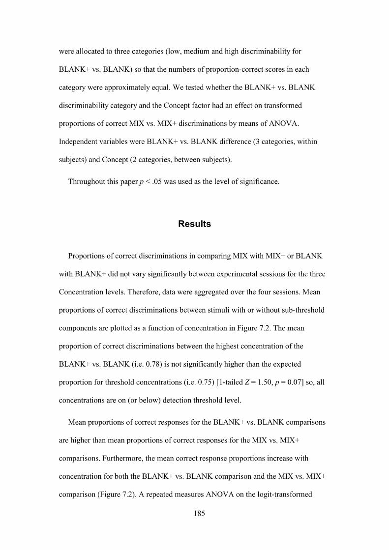
185
were allocated to three categories (low, medium and high discriminability for
BLANK+ vs. BLANK) so that the numbers of proportion-correct scores in each
category were approximately equal. We tested whether the BLANK+ vs. BLANK
discriminability category and the Concept factor had an effect on transformed
proportions of correct MIX vs. MIX+ discriminations by means of ANOVA.
Independent variables were BLANK+ vs. BLANK difference (3 categories, within
subjects) and Concept (2 categories, between subjects).
Throughout this paper p < .05 was used as the level of significance.
Results
Proportions of correct discriminations in comparing MIX with MIX+ or BLANK
with BLANK+ did not vary significantly between experimental sessions for the three
Concentration levels. Therefore, data were aggregated over the four sessions. Mean
proportions of correct discriminations between stimuli with or without sub-threshold
components are plotted as a function of concentration in Figure 7.2. The mean
proportion of correct discriminations between the highest concentration of the
BLANK+ vs. BLANK (i.e. 0.78) is not significantly higher than the expected
proportion for threshold concentrations (i.e. 0.75) [1-tailed Z = 1.50, p = 0.07] so, all
concentrations are on (or below) detection threshold level.
Mean proportions of correct responses for the BLANK+ vs. BLANK comparisons
are higher than mean proportions of correct responses for the MIX vs. MIX+
comparisons. Furthermore, the mean correct response proportions increase with
concentration for both the BLANK+ vs. BLANK comparison and the MIX vs. MIX+
comparison (Figure 7.2). A repeated measures ANOVA on the logit-transformed

186
proportions confirmed these outcomes by significant effects for Concentration,
[F(2,44) = 11.6, p < 0.001]; Complexity, [F(1,22) = 116.2, p < 0.001]; and their
interaction, [F(2,44) = 4.2, p < 0.05] which can be ascribed to the weaker effect that
Concentration has on discriminability in the MIX+ vs. MIX comparisons compared to
the BLANK+ vs. BLANK comparisons. An identical test for d’-converted data
revealed similar results: effect of Concentration, [F(2,44) = 12.7, p < 0.001];
Complexity, [F(1,22) = 106.6, p < 0.001]; and their interaction, [F(2,44) = 3.3, p <
0.05].
Figure 7.3 shows the proportions of correct MIX vs. MIX+ detections plotted as a
function of correct response proportions on ‘BLANK+ vs. BLANK comparisons for
the two ‘Concept’ groups. ANOVA on logit-transformed proportions did not reveal an
effect of ‘BLANK+ vs. BLANK proportion correct’ on ‘MIX vs. MIX+ proportion
correct’, [F(2,44) = 0.8. p > 0.1]. In other words: The responses on ‘BLANK+ vs.
BLANK’ comparisons do not predict the responses on the paired ‘MIX vs. MIX+’
comparisons. However, the level of concept refinement does. Subjects having highly
refined stimulus concepts (13 out of 23) scored higher proportions correct on the
‘MIX vs. MIX+’ comparisons than the subjects having poorly refined stimulus
concepts (10 out of 23) [F(1,44) = 4.6, p < 0.05]. Concept refinement was not found
to interact with BLANK+ vs. BLANK discriminabilities, [F(2,44) = 1.5, p > 0.1].
Discussion
The first objective of the present study was to compose a mixture of odorants that
reflects a natural food aroma with respect to its complexity and its perceived
familiarity. Although four SP-detected peaks could not be identified by FID, we

187
obtained a mixture generating descriptions related to apple aroma in more than half of
the subjects. Since neither visual-, nor verbal clues were given, identification
depended exclusively on the mixture’s aroma. This suggests that the mixture’s aroma
reflected the natural apple aroma rather well. Because we failed to identify several
SP-detected components, the model mixture may be expected to differ in aroma
quality from the original apple aroma. Nonetheless, we consider it acceptable to use
the present mixture aroma in studying possible causes for reconstruction discrepancy,
since merely the total absence of a distinct apple quality would interfere with the
objective to relate stimulus concept refinement to the discriminability of minor aroma
changes.

188
Proportion of correct Blank/Blank+ discriminations
0.0 0.1 0.2 0.3 0.4 0.5 0.6 0.7 0.8 0.9 1.0
Prop
ortio
n of
cor
rect
Mix
/Mix
+ di
scrim
inat
ions
0.0
0.1
0.2
0.3
0.4
0.5
0.6
0.7
0.8
0.9
1.0
Low refined stimulus conceptRefined stimulus concept
Figure 7.3. Proportions of correct MIX/MIX+ discriminations as a function of the proportion of
correct BLANK/BLANK+ discriminations and marked for the two levels of refinement of the
stimulus concept. The clustered dots represent identical proportions. The chance level for both axes
is 0.5.
Complexity
BLANK/BLANK+ MIX/MIX+
Prop
ortio
n of
cor
rect
resp
onse
s
0.0
0.2
0.4
0.6
0.8
1.0
Low Mid High
Figure 7.2. Proportions of correct discriminations (means ±±±± SEM) between mixtures with
either a sub- or peri-threshold set of components present or not. These proportions are shown
for three different concentrations (i.e. Low, Mid and High) and grouped for the two paired
Complexity manipulations.

189
The probability of detecting peri- or sub-threshold components did not increase in
the presence of a mixture of odorants representing an apple aroma. On the contrary,
the apple aroma (MIX) decreased detectability of peri- and sub-threshold components.
Although this contradicts our hypothesis that sub-threshold components could cause
the reconstruction discrepancy, this outcome is not surprising if we relate it to studies
that focus on sensory suppressive effects in mixtures. In both the olfactory and the
gustatory domain the effect of suppression of certain odour- and taste qualities by
other agents is well documented (Berglund and Olsson, 1993; Olsson, 1994;
Schifferstein and Kleykers, 1996; Schiet and Frijters, 1988; Cain et al., 1995).
Moreover, Stevens and Traverzo (1997) observed that a multi-component mixture of
tastants was more effective in masking a dissimilar tasting component than each of
the mixtures’ components was alone. In fact, their data suggest complete masking
additivity of the two masking agents that were used. When applied to the present
study, we would expect the complex apple base mixture to act as a powerful masker
for the, already nearly discriminable, sub- or peri-threshold components. The
observed suppression perfectly fits this line of expectation.
Regardless of the masking effect of MIX, the availability of a well-defined
stimulus concept was found to improve the ability to discriminate between similar
stimuli. This effect, however, was too small to counteract the suppressive influence of
the apple aroma mixture. Note that the ‘concept facilitation effect’ and the ‘mixture
suppression effect’ are unlikely to be located at the same level of stimulus processing.
Mixture suppression has been attributed to various levels of interaction, ranging from
peri-receptor levels (Ennis, 1996) to central processing levels (Rouby and Holley,
1995; Algom and Cain, 1991). Most likely, mixture suppression is due to concurrent
peripheral and central interactions (Laing and Willcox, 1987; Cain, 1975). This

190
suppression takes place during bottom-up information processing, i.e. the integration
of information from physical stimuli resulting in a cognitive representation that allows
an adequate response or further cognitive processing. In contrast, the concept
facilitation effect depends on the influence of memorised sensory representations on
the processing of the incoming stimulus information. This is an example of top-down
processing. Top-down processing is known to facilitate stimulus recognition in a
number of sensory domains. For example, the positive relation between odorants’
familiarity and discriminating ability (Rabin and Cain, 1984; Rabin, 1988; Jehl et al.,
1995) may be attributed to top-down processing. Therefore, the top-down processing
involved in concept facilitation is more central to and intrinsically different from the
bottom-up processing involved in mixture suppression.
In this study concept formation theory was proposed as the theoretical framework
from which reconstruction discrepancy can be explained. We hypothesised that sub-
and peri-threshold components can change aroma quality under the condition that the
subject has a well-refined stimulus concept. In part, this hypothesis was supported by
the results: subjects who employed a refined stimulus concept showed improved
discrimination ability. Since food aromas are familiar to many subjects, we did not
choose to manipulate the formation of stimulus concepts in a randomised
experimental design. Instead, a quasi-experiment was designed: subjects were
assigned post-hoc to either of both ‘Concept’ groups according to their existing
concept refinement. Since the sequence of effects was not controlled for, the design
permits an alternative conclusion on the direction of the causal relation: good
discriminators develop well-refined stimulus concepts. Nevertheless, we argue that
the hypothesised causal direction – well-refined concepts make good discriminators –
is the most plausible one. To compare a set of stimuli on a sensory property, a subject

191
has to employ (meta-) knowledge of stimulus properties and, therefore, discriminating
processes can not occur without the involvement of cognition. Since sensory
discriminating ability starts out from cognitive processing, sheer discriminators do not
exist.
In the present case, a general conclusion should be that peri- and sub-threshold
components were not detected better in an apple-like mixture than in isolation.
However, stimulus concept refinement did affect discriminability between aromas.
For the case of the presented apple model, peri- and sub-threshold components could
account for reconstruction discrepancy, albeit with stimulus concept as a confounding
factor. The results of this study indicate that semantics are an important factor in
odour mixture research because the ecological relevance of the aroma affected its
sensory evaluation.

192
Reference List
Acree, T.E., Barnard, J. and Cunningham, D.G. (1984) A procedure for the
sensory analysis of gas chromatographic effluents. Food Chem., 14, 273-286.
Algom, D. and Cain, W.S. (1991) Remembered odors and mental mixtures:
Tapping reservoirs of olfactory knowledge. J.Exp.Psychol.Human
Percept.Perform., 17, 1104-1119.
Berglund, B. and Olsson, M.J. (1993) Odor-intensity interaction in binary
mixtures. J.Exp.Psychol.Human Percept.Perform., 19, 302-314.
Blank, I., Sen, A. and Grosch, W. (1992) Potent odorants of the roasted powder
and brew of arabica coffee. Z.Lebensmittel-Untersuch.u.Forsch., 195, 239-
245.
Bult, J.H.F., Van Putten, B., Schifferstein, H.N.J., Roozen, J.P., Voragen,
A.G.J. and Kroeze, J.H.A. A stochastic model for gas chromatography
olfactometric detection frequencies. (in preparation)
Cain, W.S. (1975) Odor intensity: Mixtures and masking. Chem.Senses Flav., 1,
339-352.
Cain, W.S., Schiet, F.T., Olsson, M.J. and De Wijk, R.A. (1995) Comparison of
models of odor interaction. Chem.Senses, 20, 625-637.

193
Czerny, M., Mayer, F. and Grosch, W. (1999) Sensory study on the character
impact odorants of roasted arabica coffee. J.Agric.Food Chem., 47, 695-699.
David, H.A. and Trivedi, M.C. (1962) Technical Report 55. Department of
Statistics, Virginia Polytechnic Institute, Blacksburg, VA.
Dravnieks, A. (1985) Atlas of odor character profiles. American Society for
Testing and Materials, Baltimore, M.D.
Dravnieks, A. and O'Donnell, A. (1971) Principles and some techniques of high-
resolution headspace analysis. J.Agric.Food Chem., 19, 1049-1056.
Ennis, D.M. (1990) Relative power of difference testing methods in sensory
evaluation. Food Technol., 44, 114-117.
Ennis, D.M. (1993) The power of sensory discrimination methods. J.Sensory Stud.,
8, 353-370.
Ennis, D.M. (1996) A general molecular model for the effect of multicomponent
mixtures on biological systems. Food Chem., 56, 329-335.
Flath, R.A., Black, D.R., Guadagni, D.G., McFadden, W.H. and Schultz, T.H.
(1967) Identification and organoleptic evaluation of compounds in delicious
apple essence. J.Agric.Food Chem., 15, 29-35.
Guadagni, D.G., Buttery, R.G., Okano, S. and Burr, H.K. (1963) Additive
effect of sub-threshold concentrations of some organic compounds associated
with food aromas. Nature, 200, 1288-1289.
194
Guth, H. (1997) Quantitation and sensory studies of character impact odorants of
different white wine varieties. J.Agric.Food Chem., 45, 3027-3032.
Guth, H. and Grosch, W. (1994) Identification of the character impact odorants of
stewed beef juice by instrumental analyses and sensory studies. J.Agric.Food
Chem., 42, 2862-2866.
Jehl, C., Royet, J.P. and Holley, A. (1995) Odor discrimination and recognition
memory as a function of familiarization. Percept.Psychophys., 57, 1002-1011.
Laing, D.G. and Glemarec, A. (1992) Selective attention and the perceptual
analysis of odor mixtures. Physiol.Behav., 52, 1047-1053.
Laing, D.G. and Willcox, M.E. (1987) An investigation of the mechanisms of
odor suppression using physical and dichorhinic mixtures. Behavioural Brain
Research, 26, 79-87.
Laska, M. and Hudson, R. (1991) A comparison of the detection thresholds of
odour mixtures and their components. Chem.Senses, 16, 651-662.
Laska, M., Hudson, R. and Distel, H. (1990) Sensitivity to biologically relevant
odours may exceed the sum of component thresholds. Chemoecology, 1, 139-
141.
Livermore, A. and Laing, D.G. (1998) The influence of chemical complexity on
the perception of multicomponent odor mixtures. Percept.Psychophys., 60,
650-661.
McCullagh, P. and Nelder, J.A. (1983) Generalized Linear Models. (1 ed.).
Chapman and Hall, London.

195
Miller, G.A. and Johnson-Laird, P.N. (1976) Language and Perception.
Cambridge University Press, London.
Novák, J., Goliás, J. and Drozd, J. (1981) Determination of hydrophilic volatiles
in gas-aqueous liquid systems by Grob's closed-loop strip/trap method and
standard-addition calibration. J.Chromatography, 204, 421-428.
O'Mahony, M. (1991) Descriptive Analysis and Concept Alignment. In H. T.
Lawless & B. P. Klein (Eds.), Sensory Science Theory and Applications in
Foods. Marcel Dekker, New York, pp. 223-268.
Olsson, M.J. (1994) An interaction model for odor quality and intensity.
Percept.Psychophys., 55, 363-372.
Patterson, M.Q., Stevens, J.C., Cain, W.S. and Cometto-Muñiz, J.E. (1993)
Detection thresholds for an olfactory mixture and its three constituent
compounds. Chem.Senses, 18, 723-734.
Pollien, P., Fay, L.B., Baumgartner, M. and Chaintreau, A. (1999) First attempt
of odorant quantitation using gas chromatography-olfactometry. Analyt.Chem.,
71, 5391-5397.
Pollien, P., Ott, A., Montigon, F., Baumgartner, M., Muñoz-Box, R. and
Chaintreau, A. (1997) Hyphenated headspace-gas chromatography-sniffing
technique: screening of impact odorants and quantitative aromagram.
J.Agric.Food Chem., 45, 2630-2637.
Rabin, M.D. (1988) Experience facilitates olfactory quality discrimination.
Percept.Psychophys., 44, 532-540.

196
Rabin, M.D. and Cain, W.S. (1984) Odor recognition: Familiarity, identifiablility,
and encoding consistency. J.Exp.Psychol.Learn.Mem.Cogn., 10, 316-325.
Rouby, C. and Holley, A. (1995) Temporal competition between odorants: Effect
of different time intervals on the perception of monorhinic and dichorhinic
binary mixtures. Perception, 24, 1083-1097.
Schieberle, P. and Hofmann, T. (1997) Evaluation of the character impact
odorants in fresh strawberry juice by quantitative measurements and sensory
studies on model mixtures. J.Agric.Food Chem., 45, 227-232.
Schiet, F.T. and Frijters, J.E.R. (1988) An investigation of the equiratio-mixture
model in olfactory psychophysics: A case study. Percept.Psychophys., 44 ,
304-308.
Schifferstein, H.N.J. and Kleykers, R.W.G. (1996) An empirical test of Olsson 's
Interaction model using mixtures of tastants. Chem.Senses, 21, 283-291.
SPSS V 7.5.2 [Computer Software] (1997) SPSS Inc., Chicago, Illinois.
Stevens, J.C. and Traverzo, A. (1997) Detection of a target taste in a complex
masker. Chem.Senses, 22, 529-534.
Swets, J.A. (1961) Detection theory and psychophysics: a review. Psychometrika,
26, 49-63.
Thurstone, L.L. (1927) Psychophysical analysis. Am.J.Psychol., 38, 368-389.

197
Ullrich, F. and Grosch, W. (1987) Identification of most intense volatile flavor
compounds formed during autoauxidation of linoleic acid. Z.Lebensmittel-
Untersuch.u.Forsch., 184, 277-282.
Van Ruth, S.M. and Roozen, J.P. (1994) Gas chromatography/sniffing port
analysis and sensory evaluation of commercially dried bell peppers (Capsicum
annuum) after rehydration. Food Chem., 51, 165-170.
Van Ruth, S.M., Roozen, J.P. and Cozijnsen, J.L. (1995) Volatile compounds of
rehydrated French beans, bell peppers and leeks. I. Flavour release in the
mouth and in three mouth model systems. Food Chem., 53, 15-22.
Van Ruth, S.M., Roozen, J.P. and Cozijnsen, J.L. (1996) Gas
chromatograpy/sniffing port analysis evaluated for aroma release from
rehydrated French beans (Phaseolus vulgaris). Food Chem., 56, 343-346.

198
8 Sequential effects in olfaction: an integrated
approach
Abstract
Different conceptualizations of sequential effects are discussed and integrated into
a unifying research approach. In an experiment, 4 odorants producing pairs with
identical, similar or dissimilar odor qualities were presented sequentially at ‘high’ or
‘low’ concentrations using inter-stimulus intervals (ISI) of 20, 60, or 180s. Identical
preceding stimuli decreased subsequent graphic intensity ratings and induced stimulus
contrast. Dissimilar preceding stimuli raised successive judgments without causing
stimulus contrast. Enhancing- and diminutive effects decayed for increasing ISI, with
the highest decay rate for enhancing effects. The results support a model comprising
two complementary mechanisms causing stimulus effects: chemosensory adaptation
and the adaptive property of the receptive system to emphasize qualitative contrast.
Time-series analysis of response residuals evidenced effects by previous responses
and by non-stimulus-related cognitive processes.

199
Introduction
When stimuli are presented sequentially, previous stimuli and previous responses
may influence the magnitude of the current intensity judgment. Traditionally, two
distinct conceptualizations of stimulus context, which we will refer to as global
context and local context, are used in studies of stimulus context effects. Global
stimulus context effects are observed as sustained modifications of stimulus-response
functions that remain relatively stable over successive trials within one session.
Relevant sources of global stimulus context are the proportional distribution of
preceding stimulus intensities, the stimulus spacing and the span of the range of
stimulus intensities. These factors were found to influence intensity judgments within
or across various modalities: vision (Mellers & Birnbaum, 1982), audition (Marks,
1992), taste (Schifferstein, 1995), olfaction (Hulshoff Pol et al., 1998) and taste vs.
olfaction (Rankin, 1993; Rankin & Marks, 2000; Nordin, 1994). In contrast, local
stimulus context effects, generally referred to as sequential effects, are induced by
immediately preceding stimuli or responses. As a consequence, sequential effects
have a transient character. Sequential effects are usually observed as correlations of
judgments with directly preceding judgment- or stimulus magnitudes. They have been
observed for audition (McKenna, 1984; DeCarlo & Cross, 1990), vision (Festinger et
al., 1970; Wagenaar, 1968), taste (Schifferstein, 1996), olfaction (Baird et al., 1996),
numerical stimuli (Wagner & Baird, 1981), haptic stimuli (DeCarlo, 1994), and
mixed-modality stimuli (Ward, 1985; Baird et al., 1980). The main focus of the
present study is on these sequential effects. First, a taxonomy integrating different
sequential effects observed when using different methods is proposed. A class of

200
influential data analysis methods, called dynamic regression methods is reviewed
followed by a review of sequential effect studies in olfaction. A unifying approach to
study the anticipated sequential effects in an olfactory setting is proposed. This
approach uses aspects from dynamic regression methods and allows the identification
of mechanisms of causality. Finally, this approach is worked out in an olfactory
experiment.
A taxonomy of sequential effects
Sequential effects on intensity judgments manifest themselves in various ways.
Which class of sequential effects is observed depends usually on the chosen method
of investigation. Consequently, there is no coherent taxonomy of sequential effects. In
addition, effect descriptors are sometimes loosely defined and used inappropriately.
Therefore, we will first discuss and categorize four elementary sequential effects
together with their associated experimental method. Assimilation is the systematic
tendency of the current judgment to shift towards the relative magnitude of the
previous event (stimulus or judgment). Hence, assimilation is observed as a positive
correlation of judgments with previous event magnitudes. Instead of calculating
correlations, conditional means may also be used. In that case, assimilation follows
from high-average judgments after previous high-magnitude events and low-average
judgments after previous low-magnitude events. Contrast is the opposite of
assimilation, as judgments deviate away from the relative magnitudes of the previous
event. Therefore, contrast is observed as a negative correlation of judgment
magnitudes with previous event magnitudes. In terms of conditional means this
implies low-average judgments after previous high-magnitude events and high-
average judgments after previous low-magnitude events. We define successive
enhancement as a systematic increase of judgments due to previous events, regardless

201
of the magnitudes of these events. Furthermore, we define successive diminution as a
systematic decrease of judgments due to previous events, again regardless of the
magnitudes of the previous events. If, for instance, 0.1 ppm, 1 ppm and 10 ppm
dilutions of an orange aroma all cause an increase of the intensity judgments of a
successively presented apple aroma, then the orange aroma enhances intensity
judgments of the apple aroma. Because enhancement and diminution effects are
unconditional with respect to the magnitude of previous events, they may occur whilst
correlations of judgments with previous events remain zero.
Schifferstein and Oudejans (Schifferstein & Oudejans, 1996) performed an
illustrative study that may give a good understanding of the nature of these
elementary effects and of the pitfalls involved when studying them. They studied
effects of preceding taste solutions on the saltiness rating of a sodium chloride
solution as a function of the judged qualitative dissimilarity and the judged saltiness
intensity similarity. Preceding stimuli included water, aqueous solutions of quinine,
citric acid, sucrose, sodium chloride, and aqueous solutions of sucrose mixed with
sodium chloride. Successive enhancement of saltiness ratings was observed for all
preceding stimuli that contained no sodium chloride, with the exception of citric acid.
Although the enhancement is observed independent of the intensity of the preceding
stimulus, this effect is generally being referred to as successive contrast (Kroeze,
1983; Schifferstein & Oudejans, 1996; Schifferstein & Frijters, 1992) or sequential
contrast (Lawless, 1991; Lawless et al., 1991). Here, the term contrast relates
primarily to the source of the effect, which is the qualitative contrast between stimuli,
rather than the effect itself, which is enhancement. Nonetheless, contrast effects as
defined in the present study were also observed by Schifferstein and Oudejans. They
reported a decrease of the observed successive enhancement effect that culminated

202
into successive diminution when they increased the sodium chloride content in
preceding stimuli. Hence, increasing the sodium chloride content of stimuli caused
decreasing saltiness ratings of subsequent sodium chloride solutions, which implies a
negative correlation between previous sodium chloride concentration and the saltiness
rating of the current stimulus.
Regression models
Notwithstanding the contributions of sequential effects, a substantial part of the
variation on current intensity judgments (Rt) is introduced by the physical intensity of
the stimulus that is responded to (St). Correspondingly, previous responses at trial t-k
(Rt-k) correlate highly with previous stimulus concentrations (St-k). As a result, the
correlation between subsequent responses (Rt and Rt-k) is substantially confounded by
the correlation between Rt-k and St-k. To distinguish between the exclusive
contributions of St-k and Rt-k on Rt, Jesteadt and co-workers (Jesteadt et al., 1977)
assumed a linear multiple regression model specifying each contribution separately:
1 1
log log log log ( , )N M
t t j t j k t k tj k
R S S R j kγ α β δ ε− −= =
= + + + + ∈∑ ∑ � (16)
Here, the intercept δ is a constant related to the values on the response scale and ε
is an error term that is assumed to be Gaussian-distributed. The regression coefficients
γ, αj and βk are the weights of the variables that may contribute to the current
response: St, St-j and Rt-k respectively. If no sequential effects occur, the coefficients
αj and βk will equal zero, thus reducing the model to the log-log transform of the
psychophysical power function with exponent γ. Employing auditory stimuli, Jesteadt
and co-workers found a negative coefficient α1 and a positive coefficient β1,
suggesting that intensity judgments assimilate toward previous responses and contrast
with previous stimuli. Responses and stimuli at lags larger than 1 did not contribute

203
significantly to the multiple regression. Others reported stimulus contrast and
response assimilation effects for 1 up to 6 lags (Ward, 1979; Ward, 1982; Ward,
1985; Mori & Ward, 1990; Schifferstein & Frijters, 1992).
Response assimilation is generally found when using models of judgmental
sequential effects that include previous responses. In the various theoretical
frameworks that were proposed to explain this effect, response assimilation is
generally attributed to ‘educated guessing’ (Ward, 1979; Mori & Ward, 1990; Wagner
& Baird, 1981; Green et al., 1977; Petzold, 1981). Responses are guessed within
limits set by assumptions of randomness or stimulus probability based on recent
stimuli. Generally, these theories predict that, if intensities of previous and present
stimuli converge, the observer will increasingly rely on his previous response in the
production of the present response. This is reflected in the commonly observed
increase of correlation between consecutive responses if the observed intensity
difference of the consecutive stimuli decreases e.g. (Jesteadt et al., 1977). This
dependency is generally referred to as the second-order dependency. When plotting
the response autocorrelation as a function of intensity difference (from negative,
through zero, to positive), the second-order dependency effect typically produces an
inverted V-shaped figure.
DeCarlo and Cross (DeCarlo & Cross, 1990) noted that the stimulus contrast effect
at lag 1, often observed when using Equation 1, contradicts the typical stimulus
assimilation effect that is found when regression models are used that do not include
Rt-k as a regressor (βk = 0 for k > 0). They resolved this discrepancy by establishing
that the error term in the model comprising only the St-k regressor is autocorrelated:
1 1 1log log logt t t t tR S S e uγ α δ ρ− −= + + + + (17)

204
In this equation, logRt = δ+ γlogSt is the log-log converted psychophysical function
and St-1 is the physical intensity of the previous stimulus. The error term is
decomposed into a first-order autocorrelive part ρet-1 and a random variable ut with
zero mean and not correlated with any ut-k (k∈�+) or et-k. The parameters γ, α and ρ
are weights of the model factors. DeCarlo and Cross showed that if a positively
autocorrelated error term was not included in Equation 2, a negative St-1 coefficient
would have been obtained, suggesting a stimulus contrast effect. This was supported
by a review of a number of auditory and visual studies that presented coefficients for
Equation 1. The authors evaluated the effect of omitting the Rt-k term from the model
by recalculating the St-1 coefficients that would have resulted if Equation 2 had been
used. This resulted in a shift from negative to slightly but consistently positive St-1
coefficients, which implies a small but consistent assimilation of Rt to St-1 rather than
a stimulus contrast. The authors concluded that Equation 2 is a parsimonious model,
providing a better account of the data than Equation 1 or Equation 2 without the
autocorrelated error term. DeCarlo and Cross further suggested that the first-order
autocorrelated error term may reflect non-monitored processes such as attention,
memory, motivation or strategy that affect response behavior over more than 1 time
period. If so, the contribution of the cognitive variable to residual autocorrelation
would depend on task instruction. To test this hypothesis, subjects were instructed
either to refer to one fixed stimulus-response pair (free magnitude estimation) or to
use the immediately preceding stimulus-response pair (ratio magnitude estimation) as
a reference for current auditory intensity judgments. As predicted, ratio magnitude
estimation led to the highest contribution of the autocorrelated error term to Rt
variance.

205
Studies of sequential effects in olfaction
Studies on sequential effects in olfaction are scarce. Two studies have investigated
sequential effects for odor intensity. Baird et al. (Baird et al., 1996) reported response
assimilation of magnitude estimation judgments as indicated by positive correlations
between Rt-1 and Rt. In line with the commonly reported second-order dependencies,
response assimilation was highest if subsequent stimuli were equal. Gregson and
Paddick (Gregson & Paddick, 1975) studied sequential effects using a linear
regression model relating Rt to St-k (k∈�+) not accounting for an autocorrelated error
term. They observed contrasting effects of St-1 on Rt for separate series of eugenol or
acetophenone at various concentrations. According to the authors, these contrast
effects were probably caused by olfactory adaptation.
In addition to these studies on odor intensity, studies have been performed in
which the odor qualities varied in the sequence. Lawless (Lawless, 1991) studied the
effect of the odor quality of preceding stimuli on the intensity judgments on two
character descriptors of dihydromyrcenol (DHM). This odorant elicits an ambiguous
odor comprising both a citrus-like and a woody sensation. After initial presentation of
odorants with a predominantly citrus-like character, the woody aspect of DHM was
rated higher than after initial presentation of woody odorants. In contrast, citrus
intensity judgments of DHM were higher after initial presentation of woody odorants
than after initial presentation of citrus-like odorants. These results may either be
caused by successive enhancement after presenting a stimulus with a different
character or successive diminution after a stimulus with a similar character. Because
stimulus concentrations did not vary in this study, no conclusions can be drawn with
respect to contrast and assimilation effects.

206
Gregson (Gregson, 1983) presented binary odorant mixtures and recorded
magnitude estimates of the character descriptors of each odorant in the mixture
(indexed i and j). Judgments of each odorant’s intensity at time t in the sequence (Ri,t
and Rj,t) were modeled as functions of previous judgments and previous and present
stimulus components (Si,t-k and Sj,t-k , k∈�+). Besides a mutual mixture suppression of
the intensity of the character descriptor of one odorant by the other odorant (effects of
Si,t on Rj,t, and Sj,t on Ri,t respectively), successive diminution was observed as an
effect of each substance on ratings of it’s character descriptor for the following
stimulus (Si,t-k on Ri,t and Sj,t-k on Rj,t , respectively). In summary, these studies show
that sequential dependencies also occur for the sense of smell, and that the size and
the nature of these effects depend on both the quality and the intensity of the used
stimuli. In short, successive diminution is observed when previous stimuli are of the
same odor quality (Gregson, 1983) and contrast is found under similar circumstances
if a correlative method is used (Gregson & Paddick, 1975). Like for taste
(Schifferstein & Oudejans, 1996), either dissimilar odor qualities induce enhancement
or identical qualities induce diminution (Lawless, 1991; Lawless et al., 1991).
Assimilation appears to be a response-induced cognitive effect, whose occurrence
depends on the similarity of successive stimulus qualities (Baird et al., 1996).
From the picture that emerges from the discussed studies we distilled the following
working hypotheses with respect to olfactory sequential effects. The correlative
effects of contrast and assimilation are directly or indirectly related to stimulus
intensity variation. Contrast depends on the intensity of the previous stimulus and has
been associated with olfactory adaptation. Assimilation depends on the previous
response magnitude if intensities of two consecutive stimuli are similar and, hence, is
likely to be related to response generation processes. The level effects of successive

207
diminution and enhancement are related to variation in stimulus quality. Enhancement
is caused by dissimilar preceding stimuli and diminution is caused by identical
preceding stimuli. In line with DeCarlo and Cross (DeCarlo & Cross, 1990), we
suggest that autocorrelation of residuals is caused by cognitive factors like attention,
memory, motivation or strategy. In contrast with the suggested sources of correlative
and level sequential effects, these factors are not directly related to specific stimulus
evaluations. An overview of the hypothesized effects and their associated methods is
presented in Table 8.1.

208
The present study
In the present study, we intend to gain a better understanding of the sources of
sequential effects in olfaction by testing the above hypotheses. To accomplish this, we
present odorants sequentially, using a factorial design in which the stimulus intensity
and the similarity between subsequent stimuli are varied systematically. This design
allows the calculation of correlation effects (contrast and assimilation). However, to
calculate level effects (enhancement and diminution), it is essential to compare
observed averages against the intensity that judged stimuli would have had in the
absence of preceding stimuli. To obtain such unbiased estimates of judged intensities,
Table 8.1. Taxonomy of sequential effects that may be observed. Specified are the
experimental methods that are sensitive to the corresponding sequential effect, the task variables
that are possible sources of the effects and the hypothesized processes involved.
Sequential effect
Experimental method Hypothesized source Possible procesinvolved
Successive enhancement
conditional Rt averages for previous qualitative similarity categories
qualitative stimulus contrast
cognitive (stimuconcept compar
Successive diminution
conditional Rt averages for previous qualitative similarity categories
qualitative stimulus similarity
periphery (neuradaptation) cognitive (habit
assimilation conditional Rt averages for categories of previous event magnitudes correlating Rt with previous event magnitudes
previous judgment magnitude (identical stimulus quality)
cognitive (judgmprocesses)
contrast conditional Rt averages for categories of previous event magnitudes correlating Rt with previous event magnitudes
previous stimulus magnitude (identical stimulus quality)
periphery (neuradaptation)
residual autocorrelation
auto-correlating residuals from the best fitting model of Rt averages
mental state Cognitive (globfactors like attenmemory, motivastrategy)

209
we follow the approach used by DeCarlo (DeCarlo, 1992) to study the decay of
sequential effects in time. In an auditory task, he varied inter-stimulus intervals and
observed that St-1 assimilation decreased in time, becoming nearly absent at the
longest inter-stimulus intervals. Accordingly, we vary inter-stimulus intervals to
obtain decay functions of level effects for all degrees of similarity between a specific
stimulus and preceding stimuli of various qualities. By estimating the level of
convergence of these decay functions, the unbiased intensities of each specific
stimulus may be estimated. This design will give insight into the processes underlying
sequential effects because different decay times may indicate the involvement of
different processes. Table 8.1 shows some processes possibly involved in the
discussed sequential effects. Two distinct levels of information processing are the
peripheral and the central level. At the central level, conscious processing may be
required to some extent. Because conscious information processing is more readily
impaired by a limited processing capacity of the system than peripheral processing,
sequential effects caused by central processes may be less robust against the effects of
new stimulus presentations than sequential effects caused by peripheral processes.
The design of this experiment allows for the examination of the robustness of
sequential effects for interceding stimuli. In spite of its great explanatory potential, a
multi-factor experiment has, to our knowledge not yet been used in studies of
sequential effects.

210
Preliminary experiment: selection of odorants of three
similarity levels
In the present study we wish to manipulate the qualitative similarity of
subsequent stimuli. This section describes the selection of two pairs of stimuli that
are perceived as similar within-pairs but dissimilar between pairs. The selection
took place on the basis of chemical and perceptual dissimilarity.
Materials and Method
Subjects
Table 8.2. Substances used to make odorous stimuli, their nominal purity, their corresponding
quality descriptors and their aqueous concentrations in the preliminary and main experiment.
Com
pone
nt
Nom
inal
pur
ity
Attr
ibut
es in
the
mai
n ex
perim
ent (
trans
late
d fro
m D
utch
)
Conc
entra
tion
in p
relim
. ex
perim
ent (
µL/L
)
Conc
entra
tions
in tr
aini
ng
sess
ion
(µL/
L)
Conc
entra
tions
(Low
-H
igh)
in m
ain
expe
rimen
t (µ
L/L)
1 hexanolc > 99 5% nutsg 130 0 50 00 25 1002 methyl 1 butyl > 94% sour 7 5 7 50 7 5m
Hexanala > 98% hedgeg 2 5 3 00 1 5 6Isobutyl acetatea > 99% lacquerg 10 0 10 00 10m
Octanalc > 98% fattyh 1 0 1 00 1 0m
R (+) limoneneb > 99% orangei 40 0 45 00 22 5 902 octanonec > 99% blue 2 0 4 00 4 0m
citrald,f > 98% lemonk 1 0 1 25 0 625 2 5
Substance are obtained from: aAlldrich, bSigma, cMerck and dAcros. eSour candy is a popular hardboiled sweet in the Netherlands where it is referred to as ‘zuurtjes’. fRacemic mixture of neral and geranial. g(Bult et al., 2001), h(Rychlik et al., 1998), i(Livermore & Laing, 1996), jOdor is very similar to the odors osimilar methyl-ketones 2-heptanone and 2-nonanone which are key aroma components in blue cheese (Lubbet al., 1997), k(Kuenzel & Bahri, 1990), mConcentrations of the four components that are used as distracters

211
Employees and students from the Food Chemistry department participated
voluntarily in a panel of 10 subjects, 5 men and 5 women. Their average age was 24.1
(SD = 3.0). At the day of the experiment, subjects were not allowed to eat spicy food
or to use any fragrance.
Stimuli
Eight substances were selected so that the odors varied from very similar to very
dissimilar. Approximately equally intense stimulus concentrations were obtained after
preliminary consultation of 10 co-workers at the faculty using an intensity-ranking
task. Initial concentrations were adjusted in an iterative way according to the average
ranks of the eight substances after each of two sessions. The resulting stimuli had
moderate intensities that were well above threshold. All but one substance were
dissolved in distilled water according to the concentrations mentioned in Table 8.2. At
room temperature, the given solution concentration of R-(+)-limonene could not be
achieved in water. Therefore, this substance was prepared as an oil-in-water emulsion
using a high-speed blender (Ultra Turrax T25, Janke & Kunkel IKA labortechnik) at
20,500 min-1 during 60 s. Assuming that headspace concentrations of dissolved
components depend on molecular diffusion at the interface between the water phase
and the headspace, emulsions will produce headspace concentrations proportional to
the concentration dissolved in water, and not to the amount present in oily volume
elements in the emulsion. Nevertheless, stimulus intensity is still related to the total
amount of oil fraction in the emulsion due to eddy diffusion (De Roos, 2000). Hence,
the chosen stimulus preparation of R-(+)-limonene allowed manipulation of stimulus
intensities above the maximum solubility in water. To prevent aggregation of oily
volume elements in the emulsion, R-(+)-limonene stimuli were prepared within one
hour prior to presentation. The emulsion could not be discriminated visually from

212
other stimuli, as was confirmed by interviewing subjects after the experiment. Except
for R-(+)-limonene, solutions were prepared and stored in the dark at 4 ºC for 16
hours and poured into presentation jars 2 hours before each session.
Procedure
Subjects were seated in individually ventilated booths. Stimuli were presented
in 200-mL glass jars that were closed by low-odor plastic screw caps. Each jar
contained approximately 10 ml of solution. To prevent exchange of volatile
components between the screw caps and the headspace, the jars were sealed with
aluminium foil before being capped. Stimuli of eight different qualities were
presented in pairs, each pair comprising two different qualities. All subjects
received all 28 possible stimulus pairs. The order of stimuli in a pair and the order
of pairs in the experiment were randomized per subject.
The subjects opened stimulus jars by unscrewing the caps while keeping the jars
just underneath their noses. Immediately after opening the jar, they took one or a few
shallow sniffs and closed the jar. They were not allowed to evaluate a stimulus twice.
Subjects could proceed in a free-paced manner to the second stimulus of each pair.
After sniffing the second stimulus, subjects judged the qualitative difference of the
pair using a 150-mm graphic rating scale presented on a laptop computer screen. The
left end of the scale was labeled ‘very similar’ and the right end was labeled ‘very
dissimilar’. Any intensity differences, if perceived, were to be disregarded. Forty-five
seconds after filling in their response, the computer screen signaled that subjects
could proceed with the next pair.
Stimulus intensities had been matched before the start of the experiment. Because
new panelists participated in this study, we double-checked the equi-intensity

213
assumption. Therefore, after finishing the dissimilarity-rating task, the subjects ranked
the 8 stimuli according to their perceived intensities.
Statistical analyses
Perceived dissimilarities were assumed to be independent of the order of stimulus
presentation. Hence, each combination of two stimuli was presented in one arbitrary,
randomly selected order, after which the inverse order of this pair was assigned the
same dissimilarity score. Dissimilarities between identical stimuli were assumed zero.
For each subject, dissimilarity scores were tabulated in an 8×8 square-symmetrical
distance matrix. The dissimilarity matrices were used to estimate disparities between
the eight odors in a group multidimensional Euclidean space using the Alscal
multidimensional scaling algorithm in SPSS. Distance scores were treated as ordinal
measures. The fit of the multidimensional model is expressed by Young’s S-stress
criterion, which is 0 for perfect fit and 1 for the worst possible fit. Results of the
stimulus intensity-ranking test were subjected to the Kruskal-Wallis test of rank
equality. Throughout this study a significance level of 0.05 is used.
Results
Multidimensional distance models were estimated from individual dissimilarity
scores of the stimulus pairs. Subsequent S-stress scores for 1-, 2-, 3-, 4- and 5-
dimensional models were 0.49, 0.29, 0.20, 0.13 and 0.09 respectively. Although
stress-improvement is still considerable when the dimensionality of the model is
raised from 3 to 4, we used the three-dimensional model (Figure 8.1) because the
number of subjects used (10) does not allow for a reliable estimation of associations at
higher dimensions (Kruskal & Wish, 1978). The disparities for the odorants in three-
dimensional space were used to calculate Euclidean distances between stimulus

214
projections on three dimensions (Table 8.3). Large distances represent dissimilar
odorants whereas small distances represent similar odorants. Pairs of odorants that
showed the smallest distances were selected as similar odorant pairs (distance ranks 1
and 2). This resulted in the selection of the similar pairs citral – R-(+)-limonene and
1-hexanol – hexanal. Odorants from different pairs showed inter-odorant distance
ranks 12, 18, 16 and 22 (out of 28 ranked distances).
Individual scores on the stimulus intensity-ranking task did not yield averaged
ranks that differed significantly [Kruskal-Wallis statistic H(7) = 9.016, p = 0.251].
Therefore, we considered the used concentrations (Table 8.2, column five)
approximately equally intense.

215
Table 8.3. Euclidean distances between odorants as derived from the best fit 3-dimensional MDS solution in the preliminary experiment. Small distances represent similar odorants, whereas large distances represent dissimilar odorants. Indices are rankings of the respective distances from smallest (1) to largest (28).
hexanol
methyl but
octanone
Citral
hexanal
Iso-but acet
limonene
octan
Hexanol 0 2.16 1.72 2.61(12)
0.96(2) 2.99 2.80(16) 2.38
Methyl but
0 1.98 2.99 2.86 1.19 2.87 2.17
Octanone 0 2.95 2.67 2.68 3.24 3.50
Citral 0 2.83(1
8) 2.72 0.62(1) 3.13
Hexanal 0 3.60 2.97(22) 2.26
Iso-but acet
0 2.46 2.56
Limonene
0 2.81
Octanal 0
Figure 8.1. Three-dimensional MDS solution for the eight stimuli used in the preliminary experiment. Small disparities represent similar odorants, large disparities represent dissimilar odorants. Euclidean distances within and between the two clusters of similar components are given in Table 8.3.
-2,0-1,5-1,0-0,50,00,51,01,52,0
-2,0-1,5-1,0-0,50,00,51,01,5
-2,0
-1,5
-1,0
-0,5
0,0
0,5
1,0
1,5
Dim
ensi
on 3
Dimension 1
Dim
ensi
on 2
o enonatc
lartic
lonaxeh
lanaxeh
enenomil
tub-htem
ca-tubosi
lanatco
216
Main Experiment
Materials and Method
Subjects
Fifteen paid subjects, six men and nine women, average age 27.4 years (SD = 9.5),
participated in the experiment. All subjects, recruited from the local Wageningen
community, were selected on basis of their ability to generate refined odor attributes
and their ability to use intensity scales consistently. All were non-smokers and none
suffered from olfactory disorders. Subjects gave informed consent. They were naïve
with respect to the objectives of the experiment. All subjects except one had
experience in olfactory experiments.
Stimuli
The four equally intense substances that were selected in the preliminary
experiment were used to form two sets of two substances that are qualitatively similar
within, but dissimilar between sets. Four other substances of the same intensity were
added as distracting stimuli. The concentrations of the experimental stimuli were
multiplied and divided by two, to obtain high and low concentrations. Resulting
stimulus concentrations of the eight experimental stimuli and the four distracters are
given in Table 8.2. Stimuli were prepared as described in the method section of the
preliminary experiment.
Stimulus sequencing
Stimulus sequences varied on three factors: stimulus quality (Quality, 4 levels:
citral, R-(+)-limonene, 1-hexanol and hexanal), stimulus intensity (Intensity, 2 levels:

217
High and Low) and ISI (3 levels: 20 s, 60 s and 180 s). A stimulus sequence can be
conceived of as a series of consecutive stimulus pairs:
1 2 3 1 1 1
1 2 2 3 1 1 1
Sequence: ... ...
Pairs:
k k n n
k k n n n
S S S S S S S S
S S S S S S S S S S
+ −
+ −
⇓ ⇓ ⇓ ⇓ ⇓
where Si is the ith stimulus in the sequence. Within each full sequence, the stimulus
pairs comprised all possible combinations of Quality, Intensity and ISI. Four different
odor qualities at two intensities per quality resulted in 8 different stimuli. Allowing
for identical stimulus pairs, these combined to 82 = 64 different sequences of two
stimuli. Combining all unique pairs with the three ISIs resulted in 192 unique Sk-ISIk-
Sk+1 combinations. For each subject, a computer algorithm generated a unique random
stimulus sequence by randomly generating ISI-stimulus combinations and selecting
only those that met the requirements of a full factorial design of pairs at lag 1. This
sequence was split up into six consecutive sections that were presented at separate
sessions during a three-week period. If consecutive sections are presented on different
occasions, sequential effects are not transferred over the intersections. To prevent
these discontinuities, sections were preceded by repetitions of the last four ISI-
stimulus combinations of the preceding section. At the first session, the last four ISI-
stimulus combinations of the last section preceded the section presented. As a result,
each person’s stimulus sequence could be conceived as a circular sequence with each
of the 192 different ISI-stimulus combinations being preceded by at least four stimuli.
We did not use responses to the four ‘warm-up’ stimuli in our analyses. This
procedure also excludes responses generated while adopting a response strategy
(Schifferstein & Kuiper, 1997), inclusion of which could harm stationarity of
response data.

218
Although only responses to four different stimulus qualities were used for data
analysis, the subjects were to anticipate any of 8 different stimulus qualities at any
time. This was done to increase task difficulty. Four extra qualities of distracter
stimuli were added to the sequences at each session. To ensure that these distracter
stimuli did not influence performance on the main task, they were appended before (3
distracters) and after (1 distracter) the main sequence. Each session lasted
approximately one hour. An example of a full stimulus sequence using two odor
qualities, 2 intensities and 2 ISIs is shown in Table 8.4.
Procedure
Laboratory conditions and stimulus preparations were similar to those in the
preliminary experiment. In an approximately one-hour training session, subjects were
familiarized with the odorants and the experimental procedure. They were instructed
to sniff the eight equi-intense odorants (Table 8.2, column 5) and to memorize the
accompanying odor descriptors (Table 8.2, column 2). After memorizing odor-
descriptor associations, they had to match descriptors to the eight odors until
performance was perfect. Finally, a 30-minute version of the sequence experiment
was presented to familiarize subjects with the routine.

219
The six experimental sessions had identical procedures. First, subjects did the
Table 8.4. Example of a randomized stimulus sequence. Distracting stimuli (X1 – X4) consist of equi-intense 2-methyl-1-butyl acetate, isobutyl acetate, octanal and 2-octanone. Warm-up stimuli are repetitions of the last four stimuli in the previous session, or the last four stimuli in the final session if the current session is the first session (see the outlined sections). The experimental sequence (bold typed letters) comprises a full factorial combination of all possible binary stimulus combinations with all possible ISIs (32 stimuli in this example and 192 stimuli in the experiment). The stimuli ‘a’ and ‘A’ are low and high concentrations respectively of one substance whereas ‘b’ an 'B’ are low and high concentrations respectively of another substance. Numbers below the stimulus indices are the ISIs (s) between consecutive stimuli.
Session # Distracting
stimuli
Warm-up
stimuli
Experimental sequence Distractng
stimuli
1 X1
X2
X3
b b a a B B b A a a B X4
60
20
20
60
20
60
20
20
60
60
60
20
60
60
20
2 X1
X2
X3
A a a B a b b a A B A A b B X4
20
60
20
60
20
60
60
60
20
60
20
20
20
20
60
20
60
60
3 X1
X2
X3
A A b B b B a A b A A B B A X4
20
60
60
20
60
20
60
20
20
20
60
60
20
20
60
20
60
60
4 X1
X2
X3
A B B A a b b a a X4
20
20
60
20
60
20
60
60
60
20
60
20
20
1The intervals preceding distracting stimuli were randomly chosen from the set of intervals used inthe target sequence

220
matching test that was also used in the training session. After perfect performance was
reached, they proceeded with the main experiment. Subjects were guided by a time-
controlled computer routine that presented instructions on a 12-inch laptop color
screen at 800×600-pixel definition (Acer Extensa 501T, Pentium II). Stimulus jars in
the sequence were indexed with increasing numbers that corresponded with the
numbers of the consecutive response fields on the computer screen. Each stimulus
evaluation trial started with a grey screen showing the number of the upcoming
stimulus. The subject had to keep the jar with that number underneath his/her nose.
The jar was opened as soon as the background color of the computer screen turned to
green. When the subject started to sniff a jar, (s)he struck a key registering the time
the actual sniffing commenced. As soon as the subject was ready to indicate the
stimulus quality and intensity, (s)he struck a key again after which a screen appeared
with eight horizontal 150-mm graphic scales, each labeled on the left hand side with
one of the eight odor descriptors (Table 8.2). The left end was labeled ‘no perceivable
odor’ whereas the right end was labeled ‘extremely strong odor’. From top to bottom,
the descriptors were arranged in alphabetic order. By a single mouse click on the
appropriate scale, subjects selected an odor descriptor and rated the odor intensity.
Finally, subjects confirmed their choice by clicking a button in the response screen.
Then the next trial’s initial gray screen was shown. The signal that called for stimulus
evaluation was time-locked with the call for the former stimulus evaluation,
regardless of the in-between actions of the subject. This procedure was repeated until
the last stimulus was evaluated. As an additional check on whether the proper ISIs
were respected in the experiment, all response actions on the computer were timed
and recorded automatically.

221
Data treatment and statistical analyses
Normalization of response data. To compensate for idiosyncratic scale usage, each
subject’s responses were normalized according to:
,,
' '( ' ) '
( ' )t subj subj
t subj all allsubj
R RR SD R R
SD R −
= ⋅ +
(18)
Here, the normalized intensity score for an individual subject at time t [ ,t subjR ] is
calculated as a function of the subject’s response at time t [ ,'t subjR ], the average
response value of that subject [ 'subjR ], the standard deviation of the intensity scores of
that subject [ ( ' )subjSD R ], the standard deviation of all subjects responses [ ( ' )allSD R ]
and the average response intensity of all subjects [ 'allR ].
Calculation of residuals. In compliance with the sequential regression model of
Equation 2, we related judgments Rt to St and St-1 and not to Rt-1. To prevent confusion
with the physical stimulus concentrations St and St-1, we will specify the physical
intensity levels by It and It-1 (‘low’ or ‘high’). In this study we studied effects on
intensity judgments by the level of qualitative similarity with the previous stimulus
(QSim: identical, similar and dissimilar), It-1, It, and ISI (20 s, 60 s and 180 s). The
average panel response to a stimulus in a specific experimental condition is obtained
by calculating the average of normalized responses of panelists for that condition.
Hence, such panel averages can be interpreted as estimates of normalized responses
for individual subjects. When averaged panel responses are used as estimators of
individual responses, observed normalized responses by individual subjects may
deviate from the mean panel response due to a limited number of factors. First,
individual subjects may show different sensitivities to an odorant. This would cause
differences in the shape of subjects’ psychophysical functions and raise the inter-

222
subject variability of responses. Second, repeated evaluations by one observer of
identical stimuli in identical contexts generally result in variable judgments due to
irregularities in the transfer of the stimulus to the receptor and the transfer of
information through the perceptional system. Due to their ad hoc nature, these two
factors, i.e. inter-individual sensitivity variation and intra-individual variation of the
responsiveness of the perceptual system, will only cause uncorrelated residuals. A
third factor is the influence of cognitive variables that induce response bias,
independent of the stimulus being evaluated (DeCarlo & Cross, 1990). For instance, a
subject may be inclined to overestimate intensities during some consecutive trials as a
result of an increased task motivation. This would result in systematic changes of
response residuals over multiple stimulus evaluations (DeCarlo & Cross, 1990),
inducing a positive autocorrelation of residuals. Finally, if the proposed regression
model does not account for effects of Rt-1 on Rt , and second-order dependencies of Rt
on Rt-1 occur, then these dependencies will contribute to the residual variance.
Correlations of Rt with Rt-1 then would cause autocorrelating residuals, but only for
specific combinations of subsequent stimuli. In the present study, residual
autocorrelation effects due to cognitive factors and response autocorrelation were
studied using residuals of the full factorial QSim (3), It-1 (2), It, (2), ISI (3) and
Odorant (4) model of averages.
Conditional autocorrelation effects. Pairs of successive stimuli were categorized
according to the similarity of their intensities. Intensity similarities (ISim) of It and It-1
were either ‘identical’ (i.e. hight-1 vs. hight or lowt-1 vs. lowt) or ‘different’ (i.e. hight-1
vs. lowt or lowt-1 vs. hight). In two consecutive analyses, the dependencies of the
Pearson product moment correlations (r) between successive residuals [residual(t) and
residual(t-1)] on the joint effects of ISim and QSim and the joint effects of QSim and

223
ISI were calculated. Differences between residual correlations were then tested in a
(2×3) ISim × QSim and a (3×3) QSim × ISI repeated-measures analysis of variance.
Prior to the repeated-measures analysis, correlations were corrected for deviations
from normality by r’- transformation of individual r (Fischer, 1921) by:
1' 0.5 ln1
rrr
+ = ⋅ − (19)
Since 15 subjects produced data and because the number of within-subject
categories was - depending on the test design – either six or nine, we used univariate
tests for within-subjects effects (Stevens, 1996). Univariate test results were corrected
for non-sphericity using Greenhouse-Geisser’s epsilon. Analyses were performed
with the SPSS v10 statistical software package. For all tests, a significance level of
0.05 was used.
Results
Threats to reliability of time series analyses and external validity
Learning effects may have occurred over the six consecutive sessions. If so,
proportions of correct attribute selections, intensity judgments and, possibly, residuals
may show trends. A prerequisite for the calculation of autocorrelations, referred to as
weak stationarity, is that averages and standard deviations are constant for any
subsection of a data series (Chatfield, 1996). Thus, the occurrence of trends in
residuals over time would imply a violation of the stationarity of this data series and
harm the reliability of autocorrelation calculations. An inspection of the proportions
of correct attribute selections indicated no learning effects: over sessions, the
proportions of correct attribute selections remained constant at approximately 0.7. A
repeated measures ANOVA of logit-transformed proportions of correct scores did not

224
show significant differences between sessions [F(5,70) = 0.694, p = 0.577]. Average
judgments were 42.1, 44.5, 46.2, 41.2, 41.0, 44.3 (for sessions 1 – 6 respectively) for
low concentrated stimuli and 70.8, 72.6, 73.2, 68.3, 71.3, 72.3 (for sessions 1 – 6
respectively) for high concentrated stimuli. These scores did not show any trends over
sessions.
In the preliminary study, we made up sets of substances constituting odorant pairs
with different similarity qualifications. Since the panel in the preliminary study
differed from the panel in the main study, we examined whether the panel in the main
study agreed with the similarity categories. To test this, we assumed that similar
stimuli would be confused with each other more frequently than dissimilar stimuli.
This implied that the correct descriptor would be selected most frequently, and that
similar stimulus descriptors would be selected more frequently than dissimilar
descriptors. In Figure 8.2, proportions of responses on the QSim categories ‘correct’,
‘similar’ and ‘dissimilar’ are shown for the four substances. Proportions for each
distracter category are also included. For all stimulus qualities, correct responses were
most common, false identifications by using a ‘similar’ category were less common.
Despite the fact that responses were cumulated over two ‘dissimilar’ categories, these
categories received the lowest proportion of false responses. A (3 × 4) repeated-
measures analysis of variance on logit-transformed proportions of correct responses to
the three QSim categories for the four different odorants citral, R-(+)-limonene, 1-
hexanol and hexanal (Odorant) resulted in a significant main effect of QSim [F(2,28)
= 64.31, p < 0.001]. Significant effects were found for the contrasts comparing
‘correct’ with ‘similar’ proportions and ‘similar’ with ‘dissimilar’ proportions
[F(1,14) = 23.93, p < 0.001; F(1,14) = 47,29, p < 0.001 respectively]. This implies
that the probability of descriptor selection decreased with increasing dissimilarity

225
between descriptor and stimulus. A significant effect of Odorant [F(3,42)=5.44, p =
0.007] was also found. This was mainly due to the different frequencies with which
distracters were selected per odorant (Figure 8.2). The relatively high proportions of
distracter selections after presentation of 1-hexanol (Figure 8.2) also added to the
external validity of the results. These high proportions corresponded with the small
disparities between the two distracting substances octanone (‘blue cheese’) and
octanal (‘fatty’) and the target substance 1-hexanol (Table 8.3 and Figure 8.1), as they
were found in the preliminary study. No significant Odorant × QSim interaction was
found [F(6,84) = 1.36, p = 0.271].
------------------------------------------
insert Figure 2 approximately here
------------------------------------------
Effects of current stimulus intensity, former stimulus intensity, ISI and inter-
stimulus similarity on intensity judgments
Normalized intensity judgments were averaged over substances. The influences of
ISI levels (20 s, 60 s and 180 s), QSim levels (‘identical’, ‘similar’ and ‘dissimilar’), It
levels (‘high’ and ‘low’) and It-1 levels (‘high’ and ‘low’) on normalized intensity
judgments were tested within-subjects by repeated measures ANOVA. Significant
main effects were found for It-1 [F(1,14) = 12.50, p = 0.003], It [F(1,14) = 415.71, p <
0.001] and QSim [F(2,28) = 40.55, p < 0.001]. A significant interaction was found for
ISI × It [F(2,28) = 4.32, p = 0.025].
To illustrate these effects, we presented averaged responses as functions of sub-
sets of the independent variables in Figures 8.3, 8.4 and 8.5. Inspection of the mean
intensity judgments in Figure 8.3 learned that the main effect of QSim was due to
consistently lower judgments of stimuli preceded by identical stimuli. Furthermore, at

226
20 s ISI, stimuli preceded by dissimilar stimuli were judged more intense than stimuli
preceded by similar stimuli. To determine whether QSim effects on intensity
judgments reflected successive diminution or successive enhancement effects, we
assumed that sequential effects reduce to zero at sufficiently large ISI. In other words:
At infinitely large ISI, responses to a specific stimulus would all level out at a unique
judgment value, which is free from enhancement- or diminution effects due to QSim.
Hence, this asymptotic level reflects a judgment that is free from sequential effects.
To estimate the asymptotic level from the data, normalized responses were modeled
by exponential growth and decay functions of ISI:
0 , , 0 1, 0ISIISI QSim QSim ISIR R a b e a b b ISI= + ⋅ + ∈ ≤ ≤ ≥� (20)
where RISI is the response intensity at time ISI, R0 is the asymptote of the model,
representing the judgment in the absence of sequential effects at infinitely large ISI,
and eISI is an error term. The index QSim indicates the qualitative similarity between
the currently judged stimulus and the previous stimulus. In Figure 8.3, the least-sum-
of-squares model fit is superimposed on the averaged intensities across ISI × QSim
categories. It shows that intensity judgments decrease when preceded by qualitatively
identical stimuli and increase when preceded by qualitatively dissimilar stimuli. The
successive diminution effect of identical preceding stimuli can be observed from 20-s
up to 180-s ISI while the successive enhancement effect of dissimilar preceding
stimuli is only visible at 20-s ISI. When stimuli are preceded by similar stimuli, the
respective intensity judgments do not differ from the asymptotic level at any ISI. Note
that the estimated asymptotic judgment (R0 = 58.60) is higher than the average
judgment ( R = 56.16). This is caused by the massive successive diminution effect
due to identical preceding stimuli.

227
The main effects of It-1 and It are illustrated in Figure 8.4. The effect of It reflects
the obvious stimulus-response relation: Intensity judgments are lower for low
stimulus intensities than for high stimulus intensities. The effect of It-1 is caused by
higher judgments after low concentrated previous stimuli and lower judgments after
high previous stimulus intensities (Figures 8.4 and 8.5). This indicates that the
magnitude of the current judgment is negatively related to the intensity of the
previous stimulus. The interpretation of the ISI × It interaction follows from Figure
8.4. The differences between intensity judgments for low and for high concentrated
stimuli were relatively large at 20 s ISI whereas these differences were relatively
small at 180 s ISI.
------------------------------------------
insert Figures 3, 4 and 5 approximately here
------------------------------------------
The It-1 stimulus-contrast effect (Figure 8.5) appears to decrease for increasing
stimulus dissimilarity. However, the It-1 × QSim interaction was not significant
[F(2,28) = 1.76, p = 0.198]. Furthermore, the expected decay of enhancement- and
diminution effects over ISI (Figure 8.3) expressed by the ISI × QSim test was not
significant [F(4,56) = 2.10, p = 0.107]. Also the related interactions ISI × QSim × It-1
[F(4,56) = 1.98, p = 0.130] and ISI × QSim × It [F(4,56) = 2.57, p = 0.064] failed to
reach significance. Although the overall ANOVA did not show significant effects, the
ANOVA of the hypothesized linear (It-1 × QSim) contrast testing the decrease of
stimulus contrast at increasing stimulus dissimilarity and the linear (ISI × QSim)
contrast that tests convergence of intensity judgments of the three QSim categories at
increasing ISI were significant, [F(1,14) = 5.15, p = 0.040] and [F(1,14) = 12.71, p =

228
0.003], respectively. No additional second- and higher order interactions on intensity
judgments were found.
At lag 1, identical previous stimuli induced profound successive diminution effects
that sustained over ISIs up to 180 s. Even after this large ISI, the average intensity
judgment did not reach the asymptotic level (Figure 8.3). Therefore, we examined the
effects of identical preceding stimuli spanning more than one sequential step. We
averaged intensity judgments for stimuli that were preceded by identical stimuli
(regardless their intensity) at lag 1, 2 and 3, under the restriction that intermediate
stimuli had different qualities. Averages were calculated for each time interval
between two identical stimuli. Due to the increasing number of possible ISI
combinations at increasing lags, the number of time interval categories increases,
leading to fewer judgments per average. The number of judgments per average was
further limited by the restraint not to accept identical intermediate stimuli, since these
would reinforce any existing effects of the preceding stimulus of interest. At lag 4, the
average number of judgments that was used to calculate intensity averages had
dropped from 240 judgments at lag 1 to 22.4 judgments per time interval. Therefore,
data were not analyzed for lags higher than 3 (39.6 judgments per average). The three
averages with the largest standard errors at lag 3 were calculated from respectively 10,
23 and 9 judgments. Results were plotted in Figure 8.6. A reference line for zero-
enhancement is added, defined by the predicted asymptotic judgment level that was
assessed by Equation 5. Independent of the number of intermediate stimuli, intensity
judgments were well below the asymptotic level up to time intervals of approximately
180 s. Trends of intensity judgments over time intervals do not appear to be affected
by the number of interceding stimuli.
------------------------------------------

229
insert Figure 6 approximately here
------------------------------------------
Auto-correlation of residuals
Sequential dependencies of residuals were studied by calculating
autocorrelation functions of lag (ACF) and partial autocorrelation functions of lag
(PACF). The latter calculates the net autocorrelation at lags higher than one by
separately accounting for compound autocorrelations at lower lags. ACF and
PACF were calculated per subject and the significance of deviations of correlations
from zero were tested by one-sample T-tests, on r’ transforms using subjects as
source of variance. Resulting ACF and PACF are plotted in Figure 8.7. Although
autocorrelations are rather small, i.e. in between –0.1 and 0.1, they are significant
at 6 out of 16 lags. Furthermore, autocorrelations are positive at all lags, with the
exception of lag 1.
As was expected on basis of the external cognitive variable hypothesis,
autocorrelations of residuals were positive at lags higher than 1. This is also observed
for partial autocorrelations, implying that positive autocorrelations are not caused by
progressing autocorrelations at lower lags. However, at lag 1 autocorrelations were
significantly negative, a result that is not in line with the external cognitive variable
hypothesis. To test whether this negative autocorrelation of residuals at lag 1 was
induced by task related variables, we calculated autocorrelations of residuals at lag 1
for all possible combinations of present with previous stimuli separately. Thus,
secondary dependencies of residual autocorrelations were tested in a QSim × ISim ×
ISI (3×2×3) repeated-measures analysis of variance on r’-transforms of individual
autocorrelations. This analysis showed significant main effects of QSim [F(2,28) =
3.87, p = 0.035] and ISim [F(1,14) = 79.90, p < 0.001] and a significant QSim × ISim

230
interaction [F(2,28) = 5.17, p = 0.017]. Inspection of Figure 8.8 reveals that the ISim
effect is caused by a pronounced positive autocorrelation of residuals when two
subsequent stimuli are of the same intensity category vs. a negative autocorrelation of
residuals when two subsequent stimuli are of dissimilar intensity categories. On
average, autocorrelation magnitudes decreased at increasing dissimilarities of
subsequent stimulus qualities (Figures 8.8 and 8.9). Figure 8.8 suggests that the effect
of QSim is mainly due to decreasing positive autocorrelations for equal intensity
stimulus pairs when the stimuli decrease in qualitative similarity. When the intensities
in the consecutive stimuli are different, the qualitative similarity does not seem to
have an effect on autocorrelation. This explains the significant QSim × ISim
interaction. No significant effect of ISI [F(2,28) = 1.07, p = 0.345] is observed. Figure
8.9 shows no trace of the usual trend that sequential effects decrease over increasing
ISI. No further significant interactions were observed.
------------------------------------------
insert Figures 8 and 9 approximately here
------------------------------------------
Discussion
In the introduction we proposed a taxonomy of sequential effects that distinguishes
between level effects on judgment magnitudes (i.e. enhancement and diminution) and
correlative effects (i.e. assimilation and contrast). For reasons of clarity, results will
be discussed accordingly, followed by a discussion of the possible sources of the
observed effects. We conclude with discussing residual autocorrelation effects.

231
Internal validity
Data analyses were performed under the assumption that the panels employed in
the preliminary and the main experiments agreed in their perceptions of odor
similarity and that no learning effects took place between experimental sessions.
On the basis of the proportions of responses in the ‘correct’, ‘similar’ and
‘dissimilar’ categories we conclude that the panels indeed agreed in their
perceptions of odorant similarities. Since trends over sessions were observed
neither for the proportions of correct responses nor for the average intensity
judgments, we concluded that it is not likely that learning effects have affected
response behavior.
The equi-intense concentrations of the used substances, made up in the preliminary
experiment (Table 8.2), were multiplied or divided by two, to obtain a high and a low
concentration of each substance, respectively. Although low concentrations resulted
in low intensity judgments and high concentrations resulted in high intensity
judgments, the intensity differences between low and high concentrations varied
between substances: 1-hexanol = 14.2; hexanal = 24.7; citral = 36.7 and limonene =
37.1. This is probably due to differences between psychophysical functions of
different odorants. Unfortunately, the similar pair consisting of limonene and citral
showed large intensity differences between the low and the high concentrations
whereas the other similar pair (hexanal and 1-hexanol) showed small intensity
differences. Subjects may have exploited this as an aid in the descriptor selection. For
instance, observed intensities of limonene and citral differ more from single-intensity
distracters than observed intensities of hexanal and 1-hexanol. Therefore, exploitation
of intensity differences would make distracter selection less likely if limonene or
citral is presented. However, Figure 8.2 showed no clear evidence of such facilitation

232
of stimulus identification. Hence, distracter selection appeared to depend primarily on
qualitative similarities.
Sequential level effects on judged intensity
A massive successive diminution effect was observed due to preceding stimuli
with an identical chemical composition as the current stimulus. This successive
diminution decreased for increasing ISI but failed to reach asymptotic level before
180s. A sequential enhancement effect was also observed, caused by preceding
stimuli of a dissimilar quality. Full recovery from this enhancement was reached after
approximately 60s, which is considerably faster than the observed recovery from
diminution. Therefore, we expect that principally different mechanisms caused these
two sequential effects. Averaged intensity judgments appeared not to be affected by
preceding stimuli with a similar odor quality. This result may be explained in two
ways. Either enhancement and diminution both took place in a compensatory fashion
or neither took place. Because recovery times differed for enhancement and
diminution effects, regardless the initial magnitude of the effect, mutual compensation
of the two level effects was not possible at all ISI levels simultaneously. We therefore
assumed that preceding stimuli of a similar odor quality induced neither enhancement
nor diminution effects.
In the literature, successive enhancement effects are not uniformly defined. In a
taste experiment, Schifferstein and Oudejans (Schifferstein & Oudejans, 1996) used
the mean intensity judgment of a stimulus preceded by repetitions of itself as a
reference for the calculation of the successive enhancement effect that occurred when
this stimulus was preceded by repetitions of a different stimulus. Others have used the
grand mean response to a specific stimulus as the reference level. Both methods may
cause an underestimation of the reference judgment if diminution effects occur that

233
are as pronounced as in the present study. Such underestimation of the reference
judgment would cause spurious successive enhancement effects. With this in mind,
we predicted responses to stimuli at infinite ISI to calculate level effects. Nonetheless,
the presently found successive enhancement effect that was induced by only one
preceding dissimilar stimulus at an 20s ISI, was robust for this conservative
calculation method. At lag 1, intensity judgments for identical, similar and dissimilar
preceding stimuli converge at increasing ISI. This indicates that the predicted intensity
judgment at infinite ISI is a reliable reference. It is therefore improbable that the
successive diminution and enhancement effects are artifacts due to the data treatment
that was used.
Besides the temporal decay of the magnitude of both successive enhancement and
successive diminution, a temporal decay of response dynamics for It was also
observed. Responses to high, respectively low concentrated stimuli converged for
increasing ISI (Figure 8.4), resulting in a significant ISI × It interaction. Since this
effect is observed independently of other sources of two-way interactions with ISI,
e.g. QSim or It-1, we presume that this effect should be attributed to a changing
response strategy over ISI. Schifferstein and Kuiper (Schifferstein & Kuiper, 1997)
observed that when presenting sequences of taste stimuli at an ISI of 50 or 60
seconds, subjects would show incoherent response behavior over the initial 3 up to 12
trials. During these initial trials, the adoption stage, subjects are thought to adopt a
stimulus-response strategy based on the experienced sensations and the available
response scale. We suggest that in experiments that comprise variable ISIs, the
adoption of a response strategy is a continuous process characterized by a shift
towards more liberal scale usage after short ISI and increasing response conservatism
after longer ISI.

234
Correlative sequential effects
Besides the discussed successive diminution and enhancement effects, also
contrastive correlations between intensity judgments and preceding stimuli were
observed. In general, intensity judgments were significantly lower after high-intensity
preceding stimuli than after low-intensity preceding stimuli. This effect was observed
for identical preceding stimuli and to a lesser extent also for similar preceding stimuli
(Figure 8.5). In the case of dissimilar preceding stimuli, stimulus contrast is absent.
This suggests that stimulus intensity alone does not induce contrast. We conclude that,
at least to some extent, sequential contrast is a byproduct of successive diminution
effects. As we saw earlier, diminution occurs after preceding stimuli with identical
qualities. Contrast is observed when the magnitude of successive diminution depends
on the intensity of the previous stimulus.
In the present study, level effects clearly decayed over increasing ISI. In literature,
a decay of correlative sequential effects over increasing ISI has also been observed.
DeCarlo studied sequential effects on intensity judgments of 1000 kHz tones at
various sound levels (DeCarlo, 1992). Effects on coefficients and residuals of
Equation 2 were compared within-subjects for two experimental sessions employing
short (2 s-6 s) and long (15 s-20 s) inter-trial intervals (ITI). DeCarlo found St-1
assimilation effects on Rt that were larger at short ITI than at long ITI, the St-1
assimilation being nearly absent in the case of long ITI. The study by DeCarlo differs
in two important aspects from the present study. Instead of chemosensory stimuli,
DeCarlo presented auditory stimuli. Furthermore, stimuli only differed in intensity
whereas in the present study stimulus quality was also manipulated. Nonetheless,
DeCarlo’s central contention that the influence of the previous stimulus intensity
should decrease with an increase in ITI also finds support in the present study,

235
provided that DeCarlo reported assimilation whereas we found contrast. Although the
statistical test of this effect (the ISI × It-1 interaction) failed to reach significance, the
predicted trend is apparent in Figure 8.4: Independent of the current stimulus
intensity, It-1 contrast is highest for 20 s ISI (steepest downward slopes) and almost
absent for 180 s (nearly horizontal slopes).
An adaptation hypothesis of sequential effects in chemosensation
Schifferstein and Frijters (Schifferstein & Frijters, 1992) reviewed visual and
auditory experiments that used Equation 1 to calculate effects of St-1 on intensity
judgments. They calculated sequential effects for these experiments according to
Equation 2 by using the correction suggested by DeCarlo and Cross (DeCarlo &
Cross, 1990) and observed that the signs of nearly all St-1 coefficients changed from
negative into positive. Nevertheless, after correction their own taste data still
produced negative St-1 coefficients. Schifferstein and Frijters suggested that this robust
stimulus contrast is typical for the sense of taste, implying that sequential effects in
the sense of taste are at least partly mediated by processes unique for that modality.
In the olfactory domain, some authors suggested that sensory adaptation might be
such a modality-specific process causing contrast effects (Gregson & Paddick, 1975;
Lawless et al., 1991). We think that this study presents compelling evidence for the
hypothesis that chemosensory adaptation causes successive diminution and contrast.
To understand why adaptation may be an important factor causing sequential effects
in the chemical senses, it should be noted that chemosensory information transfer is
based on a physicochemical receptor interaction, whereas in other senses information
transfer is based on a physical receptor interaction. Due to the longevity of the
stimulus-receptor interaction and due to lingering of stimulus molecules in the mucus
embedding the receptor area, tastants and odorants produce sustained receptor

236
responses. In contrast, physical stimuli in the other senses are readily coded into
transient, neural responses. This may explain why in the chemical senses, as opposed
to the other senses, the exhaustion, i.e. adaptation, of receptors and/or their afferent
pathways is easily induced.
Olfactory adaptation is observed whenever the perception of a stimulus is impaired
due to sensory fatigue invoked by previous presentations. It causes decreased
perceived intensities of supra-threshold stimuli. Hence, larger decreases are observed
for more intense or lengthy adapting stimuli (Ekman et al., 1967; Berglund et al.,
1978; Cain, 1970; Cain & Polak, 1992; Todrank et al., 1991). Adaptation to an
odorant that is identical to the evaluated odorant is referred to as self-adaptation,
whereas adaptation to a chemically different odorant is referred to as cross-adaptation.
Self-adaptation generally impairs stimulus perception more than cross-adaptation
(Berglund et al., 1978; Berglund & Engen, 1993; Cain, 1970; Todrank et al., 1991).
Furthermore, cross-adaptation effects appear to be related to the perceived similarity
of the two odorants involved: increasing similarity between the adapting and the
evaluated odorant induces more adaptation (Todrank et al., 1991; Cain & Polak,
1992). Both behavioral and psycho-physiological investigations showed that, even
after a few sniffs, the olfactory system approaches full recovery from adaptation not
earlier than 60 s and up to 360 s after stimulus presentation (Stevens et al., 1989;
Morgan et al., 1997; Ekman et al., 1967; Cain, 1970; Cometto-Muñiz & Cain, 1995).
With adaptation sustaining over periods from 1 to 6 minutes and judged
stimulus intensities decreasing with increasing concentrations of the adapting
stimulus, adaptation may induce sequential effects in judgments of sequentially
presented olfactory stimuli. These sequential effects are expected to be diminutive,

237
because adaptation lowers intensity judgments, and contrastive, because adaptation
effects are larger after higher concentrated adapting stimuli.
In our study, regardless of the number of stimuli in between two identical
stimuli, the successive diminution induced by the identical preceding stimulus
disappears after approximately 3 minutes (Figure 8.6). This is a realistic recovery
period for adaptation effects. Furthermore, as may be expected for adaptation
effects, the observed successive diminution coincided with a stimulus contrast
effect. This contrast effect decreased with increasing stimulus dissimilarity.
Finally, the observed successive diminution effects were robust for interceding
stimulus presentations (Figure 8.6). Because peripheral neural fatigue is not likely
to be overruled by new stimulus presentations, in contrast with effects with a
cognitive origin, this result provides extra support for a peripheral hypothesis of
diminution effects.
A complementary mechanism for successive enhancement
Earlier, we suggested that two complementary mechanisms were responsible for
the successive diminution and enhancement effects, respectively. Diminution effects
could be attributed to a peripheral adaptation process. We suggest that the observed
successive enhancement effects can be explained by an ecologically adaptive
mechanism emphasizing new and contrasting information. For mammals, a primary
function of olfaction is to warn the organism for potential danger (Jones & Roper,
1997), for instance by (Sullivan et al., 1998; Terlouw et al., 1998)increasing vigilance
on perception of new odors (Warm et al., 1991; Warm et al., 1989). Perceptual
mechanisms that emphasize contrasting or new information play an important role in
this. For instance, to facilitate the perception of objects, visual contrast enhancement
is achieved by the lateral inhibition of ganglion- and cortical cells. We suggest that

238
the presently observed successive enhancement is an adaptive response to the
qualitative contrast (dissimilarity) between an odorant and its precursor.
Because no enhancement or diminution was observed at any ISI after stimuli with
a ‘similar’ odor quality, we concluded that after preceding stimuli of ‘similar’ odor
quality none of the two discussed complementary mechanisms was involved in the
response production. However, the It-1 contrast effect observed for ‘similar’ preceding
stimuli (Figure 8.5) still indicates a possible involvement of adaptation processes. The
mechanism causing successive enhancement only produces successive enhancement,
which may have compensated diminution effects by adaptation but not its contrast
effects (see the average intensities for high and low It-1 of dissimilar preceding stimuli
in Figure 8.5). Unfortunately, the present results do not allow a more critical testing of
these rivaling explanations.
Alternative sources of the observed sequential effects
An alternative mechanism that could cause successive diminution is stimulus
habituation. Repetitious presentations of a stimulus with inter-stimulus intervals that
are sufficiently long to prevent adaptation may still habituate the observer to that
stimulus (Kroeze, 1983). As a consequence, responses to a habituated stimulus may
be lower than responses to the same, but not habituated stimulus. Although adaptation
and habituation may both reduce judged intensities, the former acts at peripheral
levels of processing whereas the latter acts at central levels of information processing.
Therefore, adaptation effects can be introduced by merely one preceding stimulus,
whereas habituation requires repetitious exposure to the same stimulus. In an
experiment where stimulus solutions were applied directly to the observer’s tongue,
Kroeze observed pronounced habituation to sweet taste (Kroeze, 1983). However, in a
similar study employing identical ISIs and identical stimuli but an active sip-and-spit
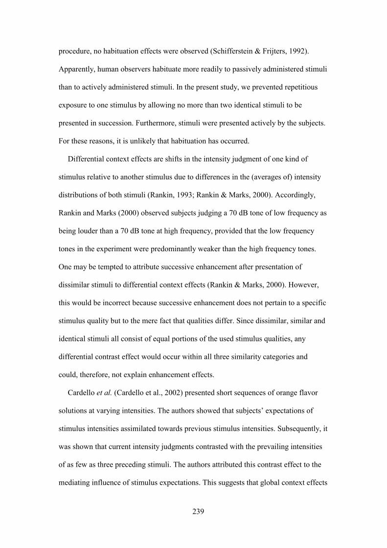
239
procedure, no habituation effects were observed (Schifferstein & Frijters, 1992).
Apparently, human observers habituate more readily to passively administered stimuli
than to actively administered stimuli. In the present study, we prevented repetitious
exposure to one stimulus by allowing no more than two identical stimuli to be
presented in succession. Furthermore, stimuli were presented actively by the subjects.
For these reasons, it is unlikely that habituation has occurred.
Differential context effects are shifts in the intensity judgment of one kind of
stimulus relative to another stimulus due to differences in the (averages of) intensity
distributions of both stimuli (Rankin, 1993; Rankin & Marks, 2000). Accordingly,
Rankin and Marks (2000) observed subjects judging a 70 dB tone of low frequency as
being louder than a 70 dB tone at high frequency, provided that the low frequency
tones in the experiment were predominantly weaker than the high frequency tones.
One may be tempted to attribute successive enhancement after presentation of
dissimilar stimuli to differential context effects (Rankin & Marks, 2000). However,
this would be incorrect because successive enhancement does not pertain to a specific
stimulus quality but to the mere fact that qualities differ. Since dissimilar, similar and
identical stimuli all consist of equal portions of the used stimulus qualities, any
differential contrast effect would occur within all three similarity categories and
could, therefore, not explain enhancement effects.
Cardello et al. (Cardello et al., 2002) presented short sequences of orange flavor
solutions at varying intensities. The authors showed that subjects’ expectations of
stimulus intensities assimilated towards previous stimulus intensities. Subsequently, it
was shown that current intensity judgments contrasted with the prevailing intensities
of as few as three preceding stimuli. The authors attributed this contrast effect to the
mediating influence of stimulus expectations. This suggests that global context effects

240
mediated by stimulus expectations can be introduced by small subsets of stimuli. With
cognitive factors like expectations being transient along trial sequences rather than
sustained, correlative effects may very well be induced. One may wonder if, for
instance, expectations could have contributed to the contrast effects that were
observed in this study.
Autocorrelation of residuals of intensity judgments at lag 1
In line with DeCarlo and Cross (DeCarlo & Cross, 1990), we assumed that
response assimilation effects are artifacts that can be attributed to autocorrelation of
residuals. DeCarlo and Cross suggested that autocorrelated residuals reflect non-
monitored processes such as attention, memory, motivation or strategy. Support for
this was found in the present study by the exclusively positive autocorrelations at lag
2 and higher. However, the observed dependency of residual autocorrelations at lag 1
on the intensity difference between the present and the preceding stimuli implies that
autocorrelation of residuals was in fact influenced by stimulus characteristics. These
stimulus-specific second-order dependencies of residuals on previous stimulus
characteristics may be explained by response assimilation or contrast effects. To
illustrate this, we discuss an olfactory study by Baird et al. (Baird et al., 1996). These
authors reported response assimilation and second-order dependencies evidenced by
an inverted V plot of correlations between Rt-1 and Rt with maximum correlations for
identical stimulus pairs. If Equation 2 had been used to model their data, then the
response variance that was originally explained by a positive autocorrelation of
responses in Equation 1 would contribute to the variance of residuals, which would
consequently be positively autocorrelated. Therefore, the observed second-order
dependency of residual autocorrelation on stimulus intensity similarity may reflect

241
sequential response effects. These occur independently of residual autocorrelations
due to stimulus-independent cognitive variables.
Besides the secondary dependency of residual autocorrelations on stimulus
intensity category, a dependency on qualitative stimulus similarity is also observed.
Residuals showed highest autocorrelations if respective stimuli had the qualitatively
highest similarity (= identical) and residuals were lowest if respective stimuli had the
qualitatively lowest similarity (= dissimilar). As with the effects of intensity
similarity, this result fitted the hypothesis that subjects relied increasingly on previous
responses when consecutive stimulus qualities were perceived as more similar.
Implications for aroma research
The present study was inspired by a research paradigm commonly used in the
realm of food aroma research and practiced at our laboratory. Food aromas generally
emanate from complex mixtures of volatile chemicals, not all of which contribute to
the aroma (Grosch, 2001). Gas chromatography olfactometry (GCO) is used to
identify the volatiles that elicit odor sensations (Abbott et al., 1993; Blank et al., 1992;
Flath et al., 1967; Gasser & Grosch, 1988; McDaniel et al., 1990; Ong & Acree, 1998;
Schieberle & Grosch, 1985; Van Ruth & Roozen, 1994; Bult et al., 2001). With gas
chromatography, a mixture of volatiles is forced through a capillary column using an
inert gas as vehicle. The retention time of each chemical component on the column
depends on its unique physicochemical interaction with the column lining, thus
causing components to elute separately in time. Retention time and chemical identity
can be monitored with detectors placed at the outlet of the column. Since human
olfactory sensitivity varies greatly over odorants (Van Gemert & Nettenbreijer, 1977),
analytical measures of concentrations of volatiles are poor indicators of their odor
impact. Therefore, human observers are used to evaluate the odors of column

242
effluents, which is the essence of GCO (Dravnieks & O'Donnell, 1971). In GCO,
human observers are generally conceived of as detectors that, ideally, generate
unbiased responses to the presented volatiles. However, as the present study indicates,
GCO results may be affected by sequential effects. An extra complicating factor is
that these effects are very complex to be understood due to the involvement of
different stimulus qualities, stimulus intensities and ISI. GCO encompasses the
presentation of relatively few, generally no more than 10 to 20 odorants. In studies
that involve a sequential presentation of stimuli, the number of initial presentations
during which subjects develop a response strategy amounts up to 12 (Schifferstein,
1996; Schifferstein & Kuiper, 1997). A straightforward estimation of the nature of
sequential effects in GCO can therefore not be given. However, intensity reduction
due to preceding stimuli is likely to occur whenever retention times of gas
chromatograph effluents differ only seconds in time whilst components are
structurally and perceptually very similar. As a matter of fact, structurally related, and
therefore often also perceptually related components tend to have similar retention
times. This makes sequential effects a probable thread to the validity of GCO
evaluations.
General conclusion
In the present study we attempted to gain a better understanding of the sources of
sequential effects in olfaction. To accomplish this, odorants were presented
sequentially whilst three factors were varied systematically: (i) the qualitative
similarity of subsequent stimulus qualities, (ii) the stimulus concentration and (iii) the
length of the ISI between subsequent stimuli. To our knowledge, sequential effects on
judgments of stimuli from different categories of odor similarity have not been
studied so far. The used multi-factor approach including ISI has proven to be a

243
powerful technique to disentangle various kinds of sequential effects and allowed the
attribution of these effects to physiological and psychological mechanisms to some
extent.

244

245

246

247
Figure legends
Figure 8.2. Average proportions of descriptors (±SEM) that were selected on presentation of
the four odorants in the main experiment. The four substances are indicated on the abscissa. Plain
bars represent ‘correct’, ‘similar’ and ‘dissimilar’ descriptor categories. Striped bars represent
distracter categories.
Figure 8.3. Average intensities (±SEM) of stimuli that were preceded by identical, similar or
dissimilar stimuli as a function of ISI. Intensities, indicated by symbols, are averaged over both It-
1 categories. Lines are best-fit exponential models as given in Equation 4.
Figure 8.4. Average intensity judgments (±SEM) as a function of the intensity category of the
preceding stimulus (It-1), the inter-stimulus interval (ISI) and the intensity category of the judged
stimulus (It).
Figure 8.5 Average intensity judgments (±SEM) of stimuli that are preceded by identical,
similar and dissimilar stimuli at both low- and high stimulus intensities.
Figure 8.6. Average intensity judgments (±SEM) of stimuli that are preceded by identical
stimuli, without any interceding stimuli (lag=1), with one non-identical interceding stimulus
(lag=2) or with two non-identical interceding stimuli (lag=3). Average judgments are plotted as a
function of the total time that elapsed after presentation of the previous stimulus with an identical
odor quality.
Figure 8.7. Autocorrelation function (ACF) and partial autocorrelation function (PACF) of
residuals (* = significant at α = 0.05).
Figure 8.8. Secondary dependencies of residual autocorrelations at lag 1 on qualitative
similarity (QSim) and similarity of intensity categories (ISim) of successive stimuli.
Figure 8.9. Secondary dependencies of residual autocorrelations at lag 1 on qualitative
similarity and inter-stimulus interval between successive stimuli.

248

249
Reference List
Abbott, N., Etiévant, P., Langlois, D., Lesschaeve, I., & Issanchou, S. (1993). Evaluation of the representativeness of the odor of beer extracts prior to analysis by GC eluate sniffing. Journal of Agricultural and Food Chemistry, 41, 777-780.
Baird, J.C., Berglund, B., & Olsson, M.J. (1996). Magnitude estimation of perceived odor intensity: empirical and theoretical properties. Journal of Experimental Psychology: Human Perception and Performance, 22(1), 244-255.
Baird, J.C., Green, B.G., & Luce, R.D. (1980). Variability and sequential effects in cross-modality matching of area and loudness. Journal of Experimental Psychology: Human Perception and Performance, 6(2), 277-289.
Berglund, B., Berglund, U., & Lindvall, T. (1978). Olfactory self- and cross-adaptation: effects of time of adaptation on perceived odor intensity. Sensory Processes, 2(3), 191-197.
Berglund, B., & Engen, T. (1993). A comparison of self-adaptation and cross-adaptation to odorants presented singly and in mixtures. Perception, 22, 103-111.
Blank, I., Sen, A., & Grosch, W. (1992). Potent odorants of the roasted powder and brew of arabica coffee. Zeitschrift fuer Lebensmittel Untersuchung und Forschung, 195(3), 239-245.
Bult, J.H.F., Schifferstein, H.N.J., Roozen, J.P., Voragen, A.G.J., & Kroeze, J.H.A. (2001). The influence of olfactory concept on the probability of detecting sub- and peri-threshold components in a mixture of odorants. Chemical Senses, 26, 459-469.
Cain, W.S. (1970). Odor intensity after self-adaptation and cross-adaptation. Perception & Psychophysics, 7(5), 271-275.
Cain, W.S., & Polak, E.H. (1992). Olfactory adaptation as an aspect of odor similarity. Chemical Senses, 17(5), 481-491.
Cardello, A.V., Melnick, S.M., & Rowan, P.A. (2002). Expectations as a mediating variable in context effects. In I. Taub & R. Bell (Eds.), Proceedings of the food preservation 2000 conference: Hampton,VA: Science & Technology Corporation.
Chatfield, C. (1996). The analysis of time series: an introduction. (5 ed.). London: Chapman & Hall.
Cometto-Muñiz, J.E., & Cain, W.S. (1995). Olfactory Adaptation. In R. L. Doty (Ed.), Handbook of Olfaction and Gustation. (pp. 257-281). New York: Marcel Dekker.
De Roos, K.B. (2000). Physiochemical models of flavor release from foods. In D. D. Roberts & A. J. Taylor (Eds.), Flavor Release. (pp. 126-141). Oxford University Press.
DeCarlo, L.T. (1992). Intertrial interval and sequential effects in magnitude scaling. Journal of Experimental Psychology: Human Perception and Performance, 18(4), 1080-1088.
DeCarlo, L.T. (1994). A dynamic theory of proportional judgment: context and judgment of length, heaviness, and roughness. Journal of Experimental Psychology: Human Perception and Performance, 20 (2), 372-381.

250
DeCarlo, L.T., & Cross, D.V. (1990). Sequential effects in magnitude scaling: models and theory. Journal of Experimental Psychology: General, 119(4), 375-396.
Dravnieks, A., & O'Donnell, A. (1971). Principles and some techniques of high-resolution headspace analysis. Journal of Agricultural and Food Chemistry, 19(6), 1049-1056.
Ekman, G., Berglund, B., Berglund, U., & Lindvall, T. (1967). Perceived intensity of odor as a function of time of adaptation. Scandinavian Journal of Psychology, 8, 177-186.
Festinger, L., Coren, S., & Rivers, G. (1970). The effect of attention on brightness contrast and assimilation. American Journal of Psychology, 3, 189-207.
Flath, R.A., Black, D.R., Guadagni, D.G., McFadden, W.H., & Schultz, T.H. (1967). Identification and organoleptic evaluation of compounds in delicious apple essence. Journal of Agricultural and Food Chemistry, 15(1), 29-35.
Gasser, U., & Grosch, W. (1988). Identification of volatile flavour compounds with high aroma values from cooked beef. Zeitschrift fuer Lebensmittel Untersuchung und Forschung, 186, 489-494.
Green, D.M., Luce, R.D., & Duncan, J.E. (1977). Variability and sequential effects in magnitude production and estimation of auditory intensity. Perception & Psychophysics, 22(5), 450-456.
Gregson, R.A.M. (1983). The sequential structure of odour mixture component intensity judgements. British Journal of Mathematical and Statistical Psychology, 36, 132-144.
Gregson, R.A.M., & Paddick, R.G. (1975). Linear transfer spectra for olfactory magnitude estimation sequences. Chemical Senses and Flavor, 1, 403-410.
Grosch, W. (2001). Evaluation of the key odorants of foods by dilution experiments, aroma models and omission. Chemical Senses, 26, 533-545.
Hulshoff Pol, H.E., Hijman, R., Baaré, W.F.C., & Van Ree, J.M. (1998). Effects of context on judgements of odor intensities in humans. Chemical Senses, 23, 131-135.
Jesteadt, W., Luce, R.D., & Green, D.M. (1977). Sequential effects in judgments of loudness. Journal of Experimental Psychology: Human Perception and Performance, 3(1), 92-104.
Jones, R.B., & Roper, T.J. (1997). Olfaction in the domestic fowl: a critical review. Physiology and Behavior, 62(5), 1009-1018.
Kroeze, J.H.A. (1983). Successive contrast cannot explain suppression release after repetitious exposure to one of the components of a tast mixture. Chemical Senses, 8(2), 211-223.
Kruskal, J.B., & Wish, M. (1978). Multidimensional scaling. (1 ed.). Beverly Hills, CA: Sage.
Kuenzel, K., & Bahri, D. (1990). Synthetic ingredients and food flavorings. In P. R. Ashurst (Ed.), Food Flavorings. (p. 115). New York, NY: AVI-Van Nostrand Reinhold.
Lawless, H.T. (1991). A sequential contrast effect in odor perception. Bulletin of the Psychonomic Society, 29(4), 317-319.
Lawless, H.T., Glatter, S., & Hohn, C. (1991). Context-dependent changes in the perception of odor quality. Chemical Senses, 16(4), 361-371.
Livermore, A., & Laing, D.G. (1996). Influence of training and experience on the perception of multicomponent odor mixtures. Journal of Experimental Psychology: Human Perception and Performance, 22(2), 267-277.

251
Lubbers, S., Cayot, N., & Taisant, C. (1997). Blue cheese taste intensification in process cheese products. Sciences des Aliments, 17(4), 393-402.
Marks, L.E. (1992). The slippery context effect in psychophysics: intensive, extensive, and qualitative continua. Perception & Psychophysics, 51(2), 187-198.
McDaniel, M.R., Miranda-Lopez, R., Watson, B.T., Micheals, N.J., & Libbey, L.M. (1990). Pinot noir aroma: a sensory/gas chromatographic approach. In G. Charalambous (Ed.), Flavors and off-flavors. Proceedings of the 6th International Flavor Conference, Rhethymnon, Crete, Greece: Amsterdam: Elsevier.
McKenna, F.P. (1984). Assimilation and contrast in perceptual judgments. The Quarterly Journal of Experimental Psychology, 36A, 531-548.
Mellers, B.A., & Birnbaum, M.H. (1982). Loci of contextual effects in judgment. Journal of Experimental Psychology: Human Perception and Performance, 8, 582-601.
Morgan, C.D., Covington, J.W., Geisler, M.W., Polich, J., & Murphy, C. (1997). Olfactory event-related potentials: older males demonstrate the greatest deficits. Electroencephalography and Clinical Neurophysiology, 104, 351-358.
Mori, S., & Ward, L.M. (1990). Unmasking the magnitude estimation response. Canadian Journal of Psychology, 44(1), 58-68.
Nordin, S. (1994). Context effects, reliability, and internal consistency of intermodal joint scaling. Perception & Psychophysics, 55(2), 180-189.
Ong, P.K.C., & Acree, T.E. (1998). Gas chromatography/olfactory analysis of lychee (Litchi chinesis Sonn.). Journal of Agricultural and Food Chemistry, 46(6), 2282-2286.
Petzold, P. (1981). Distance effects on sequential dependencies in categorical judgements. Journal of Experimental Psychology: Human Perception and Performance, 7(6), 1371-1385.
Rankin, K.M. (1993). Orthonasal vs. retronasal perception of odour: role in differential effects of context on taste and smell. Reports from the Department of Psychology, Stockholm University, 766, 1-15.
Rankin, K.M., & Marks, L.E. (2000). Chemosensory context effects: role of perceived similarity and neural commonality. Chemical Senses, 25, 747-759.
Rychlik, M., Schieberle, P., & Grosch, W. (1998). Compilation of odor thresholds, odor qualities and retention indices of key food odorants. (1 ed.). Garching: Deutsche Forschungsanstalt für Lebensmittelchemie and Institut für Lebensmittelchemie der Technischen Universität München.
Schieberle, P., & Grosch, W. (1985). Identification of the volatile flavour compounds of wheat bread crust - comparison with rye bread crust. Zeitschrift fuer Lebensmittel Untersuchung und Forschung, 180, 474-478.
Schifferstein, H.N.J. (1995). Contextual effects in difference judgements. Perception & Psychophysics, 57(1), 56-70.
Schifferstein, H.N.J. (1996). Cognitive factors affecting taste intensity judgements. Food Quality and Preference, 7(3/4), 167-175.
Schifferstein, H.N.J., & Frijters, J.E.R. (1992). Contextual and sequential effects on judgements of sweetness intensity. Perception & Psychophysics, 52(3), 243-255.

252
Schifferstein, H.N.J., & Frijters, J.E.R. (1992). Sweetness does not habituate during a sip-and-spit experiment. Physiology & Behavior, 51, 331-336.
Schifferstein, H.N.J., & Kuiper, W.E. (1997). Sequence effects in hedonic judgements of taste stimuli. Perception & Psychophysics, 59(6), 900-912.
Schifferstein, H.N.J., & Oudejans, I.M. (1996). Determinants of cumulative successive contrast in saltiness intensity judgments. Perception & Psychophysics, 58(5), 713-724.
Stevens, J. (1996). Applied multivariate statistics for the social sciences. (3 ed.). Mahwah, NJ: Lawrence Erlbaum.
Stevens, J.C., Cain, W.S., Schiet, F.T., & Oatley, M.W. (1989). Olfactory adaptation and recovery in old age. Perception, 18, 265-276.
Sullivan, T.E., Warm, J.S., Schefft, B.K., Dember, W.N., O'Dell, M.W., & Peterson, S.J. (1998). Effects of olfactory stimulation on the vigilance performance of individuals with brain injury. Journal of Clinical and Experimental Neuropsychology, 20(2), 227-236.
Terlouw, E.M.C., Boissy, A., & Blinet, P. (1998). Behavioural responses of cattle to the odours of blood and urine from conspecifics and to the odour of faeces from carnivores. Applied Animal Behaviour Science, 57(1-2), 9-21.
Todrank, J., Wysock, C.J., & Beauchamp, G.K. (1991). The effects of adaptation on the perception of similar and dissimilar odors. Chemical Senses, 16(5), 467-482.
Van Gemert, L.J., & Nettenbreijer, A.H. (1977). Compilation of odour threshold values in air and water. Voorburg: National Institute for Water Supply RID and Central Institute for Nutrition and Food Research TNO.
Van Ruth, S.M., & Roozen, J.P. (1994). Gas chromatography/sniffing port analysis and sensory evaluation of commercially dried bell peppers (Capsicum annuum) after rehydration. Food Chemistry, 51, 165-170.
Wagenaar, W.A. (1968). Sequential response bias in psychophysical experiments. Perception & Psychophysics, 3(5B), 364-366.
Wagner, M., & Baird, J.C. (1981). A quantitative analysis of sequential effects with numeric stimuli. Perception & Psychophysics, 29(4), 359-364.
Ward, L.M. (1979). Stimulus information and sequential dependencies in magnitude estimation and cross-modality matching. Journal of Experimental Psychology: Human Perception and Performance, 5(3), 444-459.
Ward, L.M. (1982). Mixed-modality psychophysical scaling: sequential dependencies and other properties. Perception & Psychophysics, 31(1), 53-62.
Ward, L.M. (1985). Mixed-modality psychophysical scaling: inter- and intramodality sequential dependencies as a function of lag. Perception & Psychophysics, 38(6), 512-522.
Warm, J.S., Dember, W.N., & Parasuraman, R. (1991). Effects of olfactory stimulation on performance and stress in a visual sustained attention task. Journal of the Society of Cosmetic Chemists, 42(3), 199-210.
Warm, J.S., Dember, W.N., Parasuraman, R., Gluckman, J.P., Thiemann, J.A., Munteanu, M., & Warren, C. (1989). The enhancement of sustained attention by olfactory stimulation. Bulletin of the Psychonomic Society, 27(6), 490-490.

253
Figure 1

254
Figure 2
0.0
0.1
0.2
0.3
0.4
0.5
0.6
0.7
0.8
0.9
1.0
citral (lemon) limonene (orange) hexanol (nuts) hexanal (hedge)
stimulus (descriptor)
Mea
n pr
opor
tion
of d
escr
ipto
r sel
ectio
ns (S
EM)
correct similar dissimilar blue cheese lacquer fatty sour candy

255
Figure 3
ISI (s)0 30 60 90 120 150 180
Mea
n in
tens
ity ju
dgem
ent (
0-15
0 m
m)
0
10
20
30
40
50
60
70
80
150
St-1 quality (QSim) = identicalSt-1 quality (QSim) = similarSt-1 quality (QSim) = dissimilar
predicted asymptote

256
Figure 4
It = high
It = low
It-1
low high
Mea
n in
tens
ity ju
dgem
ent (
mm
)
0
10
20
30
40
50
60
70
80
150
ISI = 20 sISI = 60 sISI = 180 s
It = high
It = low

257
Figure 5
QSimidentical similar dissimilar
Mea
n in
tens
ity ju
dgem
ent (
0-15
0 m
m)
0
10
20
30
40
50
60
70
80
150
It-1 = lowIt-1 = high
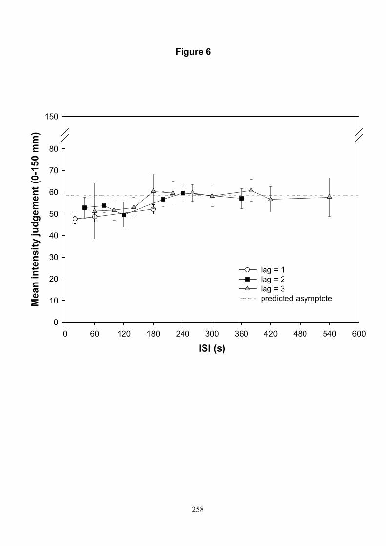
258
Figure 6
ISI (s)0 60 120 180 240 300 360 420 480 540 600
Mea
n in
tens
ity ju
dgem
ent (
0-15
0 m
m)
0
10
20
30
40
50
60
70
80
150
lag = 1lag = 2lag = 3predicted asymptote

259
Figure 7
-0.2
0.0
0.2
0.4
0.6
0.8
1.0
1 2 3 4 5 6 7 8 9 10 11 12 13 14 15 16lag
Aut
ocor
rela
tion
ACF PACF
* * ** ** * *
**

260
Figure 8
-0.5
0.0
0.5
1.0
identical similar dissimilarQualitative similarity
Aut
ocor
rela
tion
(lag
= 1)
equal intensity category different intensity category

261
Figure 9
-0.5
0.0
0.5
1.0
ISI = 20s ISI = 60s ISI = 180s
Aut
ocor
rela
tion
(lag
= 1)
identical similar dissimilar

262
9 General discussion
GCO is a method that employs panels of human detectors as an instrument to
identify the odorants in mixtures of odorous and non-odorous volatile chemical
components. As such, this method is based on paradigms from natural sciences for at
least two reasons. First, it follows the well-accepted view that complex matter may be
understood better by understanding its elements. This view suggests that decomposing
complex mixtures of odorants emanating from foods and subsequently characterising
these odorants by human detectors may provide a better understanding of the food
aroma. Second, the instrument used to quantify properties of matter should yield valid
results. Using human detectors to describe the olfactory properties of an aroma is
likely to be a valid approach. What other instrument could better describe how
humans perceive an aroma?
To detect and identify odorants, the human instrument proved both a blessing and a
curse. So far, no instruments have been constructed that can mimic the versatility and
the, at times, extreme sensitivity of humans in the detection of odorants. On the other
hand, both the psychological literature and this thesis have illustrated that the human
response depends on a multitude of factors besides the presence of the odorant alone.
Therefore, the factors that affect the validity of the human responses shoud be taken
into account when human observers are used as measuring instruments.
By approaching GCO from a combined psychological-technological perspective
this thesis work had two main objectives: (i) to use knowledge of human perception to
improve GCO methodology (the first part of this thesis) and (ii) to identify
experimental GCO conditions in which humans perform like biased instruments and

263
to study the psychological mechanisms that govern such bias (the second part of this
thesis).
The first part of this thesis
Two methodological improvements were suggested for the practice of GCO. The
first suggestion entailed the correction of panel responses for variation in
components’ retention times, due to variation in the GC instrument. This correction
improved the odorant detection power of the panel (chapter 2). Although this method
was not born from any psychological considerations, it increased the sensitivity of the
panel as an instrument. This was required before embarking on the second enterprise:
the development of a psychologically valid method to assess the reliability of panel
detections of odorants (chapters 3 and 4).
A GCO experiment is an exceptional task setting in psychological research.
Subjects have to respond to unannounced stimuli that occur after irregular time
intervals. Although this task may reflect many real life situations, e.g. noticing the
faint ringing of your cell phone inside your pocket or hearing somebody calling for
help, it is not a common situation in psychological laboratories. Here, detection
experiments generally require subjects to respond to events that occur in well-defined
time frames. Subjects are typically asked whether an event took place or not, rather
than when it took place. Chapter 3 of this thesis presented a model of detection
behaviour under unstructured tasks conditions. It models panel behaviour from
responses that were generated during time windows in which stimuli were absent.
With this model, it can be tested whether panel responses differ significantly from
those expected under stimulus-free conditions. The method proved very useful for
GCO applications and offers an ecologically valid alternative for signal detection

264
theory, the prevalent framework in the psychology of detection. Hence, the method
used to model GCO sessions may be applied in other contexts relevant to psychology
as well.
The second part of this thesis
When panellists rate stimulus intensity, characterise stimulus quality or even
indicate the mere presence of stimuli, their responses depend on a multitude of factors
besides the stimuli alone. Several relevant factors were identified earlier: stimulus
frequency (Schifferstein and Frijters, 1992; Riskey et al., 1979; Colquhoun and Baddeley, 1964);
the stimulus context as provided by task instruction (Frandsen et al., 2003; Herz and
Von Clef, 2001; Herz, 2003) and the intensity and quality of the previous stimulus in
combination with the time that has elapsed since its presentation (Ekman et al., 1967;
Cain, 1970; Bujas et al., 1991). In this thesis, the impact of such factors on odorant
perception was demonstrated in chapter 4 (stimulus frequency), chapter 6 (stimulus
context as provided by task instruction), chapter 7 (stimulus meta-knowledge), and
chapter 8 (the intensity and quality of the previous stimulus and the time that has
elapsed since its presentation). All these factors pose potential threats to the reliability
of GCO results.
Holistic stimulus perception in olfaction
For the modality of olfaction, there is compelling evidence that the neural encoding
of stimulus information is holistic as from only few synapses beyond the olfactory
bulb (Wilson and Stevenson, 2003; Wilson, 2000). Most of the detailed, odorant-
related information seems to be lost before stimulus information reaches cortical
stages of processing. Hence, complex, object-related aromas are thought to be
processed in terms of the (food) source rather than in terms of constituting odorant

265
components (Stevenson et al., 2003; Stevenson and Boakes, 2003; Stevenson, 2001).
Two studies in the present thesis dealt directly with predictions that can be derived
from this conceptualisation. In chapter 7, sub- and peri-threshold odorants were added
to a mixture of components that produced an apple aroma. Panellists found it easier to
discriminate these components in the aroma when they had recognised the aroma
(apple) than when they did not. In chapter 6, subjects proved to be better identifiers of
components in aroma mixtures when they were instructed to recognise aroma notes in
aromas of orange and apple than when they were instructed to recognise components
in mixtures of components.
The notion of holistic stimulus processing is anything but new and has been subject
of debates ever since the first experimental psychologists populated university
laboratories. In fact, it was a central point of dispute between Wilhelm Wundt, the
founder of the first psychological laboratory in 1879, and Oswald Külpe, one of his
most successful students (Leahey, 1987). Wundt was convinced that all abstract and
complex thought was constructed from simple elements that related directly to
sensory impressions. Although some complex thought could be more dominant than
its constituting parts, it still depended on sensory elements for its existence, Wundt
maintained. Hence, psychological research should deal with the study of those
elements of mental processes, whereas the direct study of higher mental processes
should be avoided for being unreliable. Külpe, on the other hand, embarked on
studying higher mental processes and concluded from these that ‘imageless’ thinking
exists. In other words, he concluded that complex mental states were possible without
a need for accessible or even existing representations of elementary stimulus input. In
the following century, this discussion reappeared in debates between extreme
atomists, who adhered to the idea that all mental processing could be reduced to

266
sensory elements, and new mentalists who believed that meaning, which was
extracted from sensory input, formed the elements of memory, to Gestalt
psychologists who claimed that every reduction of a holistic percept was artificial
(Leahey, 1987). Recent studies in olfaction, including those in the present thesis, are
supportive for the new mentalist view and even the Gestalt view with respect to
olfactory information processing.
Suggestions to improve the validity of GCO experiments
Knowing that response bias occurs does not prevent it from occurring. However, a
number of suggestions for improvement of GCO may be formulated on basis of the
findings in this thesis. Odorants that are processed sequentially influence consecutive
odorant evaluations (chapter 8). These effects were shown to be persistent over
periods of 30 seconds up to 180 seconds, depending on the mechanism involved.
Olfactory self-adaptation can only occur during the sniffing of one peak in GCO,
because each odorant is released at one retention time. Self adaptation may affect
intensity ratings but it cannot be prevented by changing GC settings. However, cross-
adaptation effects for chemically related odorants at short retention time intervals may
occur. To reduce the probability of not detecting odorants due to cross-adaptation,
intervals between odorants should preferably not be shorter than 3 minutes (see
chapter 8). In additon, to prevent sequential effects like successive contrast, any
odorant sequence with intervals below 1 minute should be prevented. If modifications
of gas chromatograph temperature programs do not enable such long intervals, it
should be considered whether GCO sessions could be split into sections that are
presented at different occasions.
Furthermore, sessions with very few noticeable odorants should be avoided. As
was shown in chapter 4, the tendency to initiate a response in olfactory detection tasks

267
increases when the apparent odorant frequency decreases to low levels. In such cases,
raising the concentration of presented volatiles might help.
In addition, it is premature to assume that ‘odour impact’ components may be
recognized on basis of their qualitative similarity to the mixture aroma or on basis of
their relatively high impact score. This thesis showed that the impact of components
on the mixture aroma could neither be based on intensity (chapter 7) nor on quality
(chapter 5). Regardless of how well trained a subject may be in recognising one
odorant, it would not necessarily mean that the subject would predict better the impact
of that odorant’s absence in the complex mixture. A better alternative for the practice
of impact component assessment is the technique introduced by (Blank et al., 1992;
Guth and Grosch, 1994; Schieberle and Hofmann, 1997). They assessed odorant
impacts by measuring the sensory implications of omitting these from the complex
mixtures.
Future research
In recent years, the issue of response reliability and method validity has been
addressed increasingly in GCO studies. Different methods of odorant impact
assessment have been compared critically (Le Guen et al., 2000; Van Ruth, 2004; Van
Ruth and O'Connor, 2001; Van Ruth, 2001) and efforts were made to assess the
reliability of odour impact scores (Pollien et al., 1997). In the absence of instrumental
methods that may replace human subjects in their sniffing task, continued efforts to
improve panel response reliability are expected. The psychological model that was
developed (chapter 3) may contribute to that development.
This thesis provided further support for the involvement of central processes in
odorant perception (chapters 6, 7 and 8). Much of this involvement could be attributed

268
to the integrative and holistic nature of aroma perception. If the contributions of
separate ingredients are lost in the process of aroma perception and replaced by one
holistic percept, one may wonder to what extent impressions from different sensory
modalities merge into holistic percepts.
Since the late 1980s, multi-modal integration processes have been studied for
odour-taste combinations. It was shown that smells may increase taste intensities or
prolong taste perceptions and vice versa (Dalton et al., 2000; Davidson et al., 1999;
Stevenson and Boakes, 1998; Frank et al., 1989; Frank and Byram, 1988). This effect
seemed to be found mainly for odour-taste combinations that co-occur in real life
(Frank and Byram, 1988), for instance strawberry odour with sweet taste. In addition,
the retronasal pathway for delivery of odorants to the olfactory epithelium, i.e. the
natural pathway during eating, favours the occurrence of multi-modal integration in
comparison with orthonasal delivery. For instance, if strawberry odour and sucrose
taste are delivered orally in an aqueous solution, swallowing leads to more sweet-taste
enhancement than the use of a sip-and-spit technique (Frank et al., 1989). This effect
is attributed to retronasally perceived strawberry odours due to the act of swallowing.
In addition, when comparing sipping an odour/taste solution with sniffing the odour
while tasting the taste solution, the relatively more retronasally presented odorants
(sipping) contribute more to perceived taste than the orthonasally sniffed odorants
(Rankin and Marks, 2000). These results support a holistic view of stimulus
perception that goes beyond the boundaries of sensory modalities.
Multi-modal interaction effects are also found for combinations of touch (texture)
and taste. A consistent finding is that by increasing the viscosity of solutions the
perceived sweetness decreases (Mackay and Valassi, 1956; Mackay, 1958;
Moskowitz and Arabie, 1970; Arabie and Moskowitz, 1971; Pangborn and

269
Szczesniak, 1974; Christensen, 1977; Christensen, 1980). One specific thickener, i.e.
acid-modified starch, introduced synergistic texture effects on sweetness perception,
which could be attributed to receptor interactions (Kanemaru et al., 2002). However,
for the general case of taste suppression by texture, it has not been proven whether
texture-taste interactions occur due to receptor interactions, e.g. the lower availability
of the sweetener due to the thickener, or whether it depends on central processes.
For the similar suppression of smell intensity by increased viscosity (Pangborn and
Szczesniak, 1974) there is convincing evidence that cross-modal effects of texture on
odour perception originate centrally: Perceived odour intensity also depends on
texture when the odorant concentration in the nose remains unchanged. (Hollowood et
al., 2002; Cook et al., 2005; Weel et al., 2002; Bult et al., 2006).
Extra support for the role of holistic perception in multi-modal integration
processes comes from neuro-physiological studies. The cross-modal integration of
taste and retronasally presented odours rely on shared cortical projections of olfactory
activations in areas that are normally activated by oral stimulation (Small et al.,
2005). Other studies, employing electro-physiological measurements (Rolls and
Baylis, 1994) demonstrated that besides the neurons responding to inputs from only
one specific stimulus modality, neurons responding to specific combinations of
stimulus modalities, e.g. odor-taste or odor-texture combinations, also exist in the
orbito-frontal cortex and other areas (De Araujo et al., 2003; Rolls and Baylis, 1994).
Small et al. (Small et al., 2004) demonstrated super-additive activations in specific
brain areas for familiar taste-odour combinations (e.g., sweet-vanilla) but not for
unfamiliar ones (e.g., salty-vanilla). It may be concluded that these studies provide
new neuro-physiological support for the central theorem of Gestalt psychology:
perceived events melt into holistic percepts that are inseparable after integration.

270
In a recent study, Bult et al. further illustrated the relevance of studying
ecologically valid combinations of stimuli from various modalities (Bult et al., 2006).
The authors showed that the separate presentation of cream odours led to perceived
increases of thickness, creaminess and flavour intensity of orally presented milks, but
only when odorants were presented retronasally. Furthermore, these intensities did not
increase when odours were presented during the filling of the mouth with the milk,
they did increase when odours were presented during oral processing of the milk and
they increased most when odours were presented during the swallowing of the milk.
This ‘presentation path’ x ‘odorant timing’ interaction suggests that texture, flavour
and even complex properties like creaminess were all influenced by a stimulus from
one modality, under the condition that the stimulus is presented under natural
presentation (path and timing) conditions. These research developments suggest that
perception studies will continue to explore the mechanisms that govern multi-modal
integration processes under ecologically valid conditions.

271
References
Arabie,P. and Moskowitz,H.R. (1971) The effects of viscosity upon perceived
sweetness. Percept. Psychophys., 9, 410-412.
Bujas,Z., Szabo,S., Ajdukovic,D. and Mayer,D. (1991) Time course of recovery
from gustatory adaptation to NaCl. Percept. Psychophys., 49, 517-521.
Bult,J.H.F., De Wijk,R.A. and Hummel,T. (2006) Investigations on multimodal
sensory integration: texture, taste, and ortho- and retronasal olfactory stimuli in
concert.
Cain,W.S. (1970) Odor intensity after self-adaptation and cross-adaptation.
Percept. Psychophys., 7, 271-275.
Christensen,C.M. (1977) Texture-taste interactions. Cereal Food World, 22, 243-
256.
Christensen,C.M. (1980) Effects of solution viscosity on perceived saltiness and
sweetness. Percept. Psychophys., 28, 347-353.
Colquhoun,W.P. and Baddeley,A.D. (1964) Role of pretest expectancy in
vigilance decrement. J. Exp. Psychol., 68, 156-160.
Cook,D.J., Hollowood,T.A., Linforth,R.S.T. and Taylor,A.J. (2005)
Correlating instrumental measurements of texture and flavour release with human
perception. Int. J. Food Sci. Nutr., 40, 631-641.

272
Dalton,P., Doolittle,N., Nagata,H. and Breslin,P.A. (2000) The merging of the
senses: integration of subthreshold taste and smell. Nature Rev. Neurosci., 3, 431-
432.
Davidson,J.M., Linforth,R.S.T., Hollowood,T.A. and Taylor,A.J. (1999) Effect
of sucrose on the perceived flavor intensity of chewing gum. J. Agric. Food Chem.,
47, 4336-4340.
De Araujo,I.E.T., Rolls,E.T., Kringelbach,M.L., McGlone,F. and Phillips,N.
(2003) Taste-olfactory convergence, and the representation of the pleasantness of
flavour, in the human brain. Eur. J. Neurosci., 18, 2059-2068.
Ekman,G., Berglund,B., Berglund,U. and Lindvall,T. (1967) Perceived
intensity of odor as a function of time of adaptation. Scand. J. Psychol., 8, 177-186.
Frandsen,L.W., Dijksterhuis,G., Brockhof,P.M., Nielsen,J.H. and Martens,M.
(2003) Subtle differences in milk: comparison of an analytical and an affective test.
Food Qual. Pref., 14, 515-526.
Frank,R.A. and Byram,J. (1988) Taste-smell interactions are tastant and
odorant dependent. Chem. Senses, 13, 445-455.
Frank,R.A., Ducheny,K. and Mize,S.J.S. (1989) Strawberry odor, but not red
color, enhances the sweetness of sucrose solutions. Chem. Senses, 14, 371-377.
Herz,R.S. (2003) The effect of verbal context on olfactory perception. J. Exp.
Psychol. Gen., 132, 595-606.
Herz,R.S. and Von Clef,J. (2001) The influence of verbal labeling on the
perception of odors: evidence for olfactory illusions? Perception, 30, 381-391.

273
Hollowood,T.A., Linforth,R.S.T. and Taylor,A.J. (2002) The effect of viscosity
on the perception of flavour. Chem. Senses, 27, 583-591.
Kanemaru,N., Harada,S. and Kasahara,Y. (2002) Enhancement of sucrose
sweetness with soluble starch in humans. Chem. Senses, 27, 67-72.
Le Guen,S., Prost,C. and Demaimay,M. (2000) Critical comparison of three
olfactometric methods for the identification of the most potent odorants in cooked
mussels (Mytilus edulis). J. Agric. Food Chem., 48, 1307-1314.
Leahey,T.H. (1987) A history of psychology: main currents in psychological
thought. Prentice-Hall, London.
Mackay,A. (1958) Discernment of taste substances as affected by solvent medium.
Food Research, 23, 580-583.
Mackay,A. and Valassi,K. (1956) The discernment of primary tastes in the
presence of different food textures. Food Technol., 10, 238-240.
Moskowitz,H.R. and Arabie,P. (1970) Taste intensity as a function of stimulus
concentration and solvent viscosity. J. Texture Stud., 1, 502-510.
Pangborn,R.M. and Szczesniak,A.S. (1974) Effect of hydrocolloids and viscosity
on flavor and odor intensities of aromatic flavor compounds. J. Texture Stud., 4, 467-
482.
Pollien,P., Ott,A., Montigon,F., Baumgartner,M., Muñoz-Box,R. and
Chaintreau,A. (1997) Hyphenated headspace-gas chromatography-sniffing
technique: screening of impact odorants and quantitative aromagram. J. Agric. Food
Chem., 45, 2630-2637.

274
Rankin,K.M. and Marks,L.E. (2000) Chemosensory context effects: role of
perceived similarity and neural commonality. Chem. Senses, 25, 747-759.
Riskey,D.R., Parducci,A. and Beauchamp,G.K. (1979) Effects of context in
judgments of sweetness and pleasantness. Percept. Psychophys., 26, 171-176.
Rolls,E.T. and Baylis,L.L. (1994) Gustatory, olfactory, and visual convergence
within the primate orbitofrontal cortex. J. Neurosci., 14, 5437-5452.
Schifferstein,H.N.J. and Frijters,J.E.R. (1992) Contextual and sequential effects
on judgements of sweetness intensity. Percept. Psychophys., 52, 243-255.
Small,D.M., Gerber,J.C., Mak,Y.E. and Hummel,T. (2005) Differential neural
responses evoked by orthonasal versus retronasal odorant perception in humans.
Neuron, 47, 593-605.
Small,D.M., Voss,J., Mak,Y.E., Simmons,K.B., Parrish,T. and Gitelman,D.
(2004) Experience-dependent neural integration of taste and smell in the human
brain. J. Neurophysiol., 92, 1892-1903.
Stevenson,R.J. (2001) Perceptual learning with odors: implications for
psychological accounts of odor quality perception. Psychon. B. Rev., 8, 708-712.
Stevenson,R.J. and Boakes,R.A. (2003) A mnemonic theory of odor perception.
Psychol. Rev., 110, 340-364.
Stevenson,R.J. and Boakes,R.A. (1998) Changes in odor sweetness resulting
from implicit learning of a simultaneous odor-sweetness association: an example of
learned synesthesia. Learn. Motiv., 29, 113-132.

275
Stevenson,R.J., Case,T.I. and Boakes,R.A. (2003) Smelling what was there:
Acquired olfactory percepts are resistant to further modification. Learn. Motiv., 34,
185-202.
Van Ruth,S.M. (2001) Methods for gas chromatography-olfactometry: a review.
Biomolecular Engineering, 17, 121-128.
Van Ruth,S.M. (2004) Evaluation of two gas chromatography-olfactometry
methods: the detection frequency and perceived intensity method. J. Chromatog.,
1054, 33-37.
Van Ruth,S.M. and O'Connor,C.H. (2001) Evaluation of three gas
chromatography-olfactometry methods:comparison of odour intensity-concentration
relationships of eight volatile compounds with sensory headspace data. Food Chem.,
74, 341-347.
Weel,K.G.C., Boelrijk,A.E.M., Alting,A.C., Van Mil,P.J., Burger,J.J.,
Gruppen,H., Voragen,A.G.J. and Smit,G. (2002) Flavor release and perception of
flavored whey protein gels: perception is determined by texture rather than by
release. J. Agric. Food Chem., 50, 5149-5155.
Wilson,D.A. (2000) Odor specificity of habituation in the rat anterior piriform
cortex. J. Neurophysiol., 83, 139-145.
Wilson,D.A. and Stevenson,R.J. (2003) The fundamental role of memory in
olfactory perception. Trends Neurosci., 26, 243-247.

276
Samenvatting behorende tot het proefschrift getiteld “Sensorische en instrumentele
analyse van voedselgeuren”
Johannes Hendrikus Fransiscus Bult
Geboren 25 november 1967 te Enschede
Levensmiddelenaromas worden in de regel als eenduidige percepten
waargenomen. Zo ruiken gebakken aardappelen naar gebakken aardappelen en ruikt
gebrande koffie naar gebrande koffie. Desalniettemin worden vrijwel alle
levensmiddelenaromas veroorzaakt door meerdere vluchtige verbindingen die in
wisselende samenstellingen aan zeer uiteenlopende aromas bijdragen. Van de
honderden vluchtige verbindingen die vrijkomen uit gebakken aardappelen en
gebrande koffie produceert een groot deel geen geur, vele tientallen produceren een
geur en dragen bij aan een van de genoemde aroma’s, vele andere aan beide aroma’s.
Desalniettemin worden voedselaromas niet als een verzameling afzonderlijke
geurende verbindingen waargenomen.
Centraal in dit proefschrift staat een methode die aangewend wordt om de
geurende verbindingen van een mengselaroma te scheiden, te identificeren en
sensorisch te karakteriseren: gas chromatografie olfactometrie (GCO). In GCO
worden vluchtige verbindingen die geïsoleerd zijn uit de gasfase die een levensmiddel
omgeeft onder druk door een capillair gevoerd. Doordat de verblijftijd in de capillair
van de verbindingen onderling verschilt kunnen proefpersonen deze bij het vrijkomen
afzonderlijk waarnemen zodat per verbinding afzonderlijke sensorische informatie
ingewonnen kan worden.

277
Panels van proefpersonen (sniffing panels) worden in
levensmiddelentechnologisch onderzoek ingezet als instrument om de geurbijdrage
van samenstellende vluchtige verbindingen vast te stellen. In de regel tracht men in
technologische studies de instrumentele foutenmarges vast te stellen en te
minimaliseren. De paradoxale situatie doet zich nu voor dat die praktijk zelden geldt
voor sniffing panels. Er is geen valide en bruikbare methodiek voor het vaststellen
van de betrouwbaarheid van panelresultaten en onderzoek naar systematische
afwijkingen van panelresponsen is er niet. Bovendien zijn een aantal aannamen die
gelden binnen GCO onderzoek psychologisch niet valide. Zo wordt algemeen
aangenomen dat sterk en prototypisch geurende verbindingen een belangrijk aandeel
in het mengselaroma zullen hebben. Waarneemstudies hebben echter aangetoond dat
gemengde geuren elkaar wederzijds kunnen onderdrukken of anderszins beïnvloeden.
Aannames voor de rol van aparte verbindingen in het mengselaroma op basis van
GCO evaluaties zijn derhalve voorbarig.
In dit proefschrift worden methodes voor het vaststellen en het verbeteren van de
betrouwbaarheid van GCO resultaten geïntroduceerd en in de praktijk getoetst
(hoofdstukken 2,3 en 4). Bovendien zijn een aantal psychologisch twijfelachtige
aannames van GCO geïdentificeerd en gebruikt als uitgangspunt voor empirische
studies. Dit heeft achtereenvolgens zijn beslag gekregen in de studie van de invloed
van stimulus context op de geschatte betrouwbaarheid van GCO resultaten (hoofdstuk
4), de invloed op mengselaroma’s van GCO-geïdentificeerde ‘character-impact’
verbindingen (hoofdstuk 5), de studie van de invloed van drempelige
geurverbindingen op bovendrempelige mengselaroma’s (hoofdstuk 6), de studie van

278
de wederzijdse beïnvloeding van sequentieel aangeboden geurstimuli op de
waargenomen geurintensiteit (hoofdstuk 7) en de studie van de invloed van
taakinstructie op de herkenbaarheid van geurverbindingen in een levensmiddelengeur
(hoofdstuk 8). Algemene conclusies zijn dat willekeurige panel responsen gebruikt
moet worden om de betrouwbaarheid van GCO geur detectie vast te stellen en dat
systematische responsvariaties gekend moeten zijn om voorbarige conclusies in GCO
te voorkomen.

279
Abstract pertaining to the thesis, entitled “Sensory and Instrumental Analysis of
Food Aromas”
Johannes Hendrikus Fransiscus Bult
Born November 25th 1967 at Enschede, The Netherlands
Food aromas are generally perceived as unitary aromas, i.e. fried potatoes smell
like fried potatoes and roasted coffee smells like roasted coffee. Nonetheless, nearly
all food aromas are produced by a multitude of volatile components that contribute to
an extensive collection of aromas in various compositions. Of the hundreds of
volatiles released from fried potatoes and roasted coffee a major selection does not
produce an odour, many others do produce an odour that contributes to one of both
aromas, many others contribute to both. In spite of this, food aromas are not being
perceived as collections of discernable odours.
Central theme of this thesis is a method used to decompose, identify and
characterise the odorous components in mixtures of odorants: gas chromatography
olfactometry (GCO). GCO entails the pressurised transfer of volatiles through a
capillary, after capturing these from the headspace surrounding a food. Since the
capillary delays volatiles differentially, panellists may sniff these volatiles
sequentially on their release from the capillary. This allows the separate sensory
evaluation of components in the aroma mixture.
A well-established practice in technological studies is that measurement reliability
of instruments is estimated and minimised. Although sniffing panels are generally

280
employed as instruments that assess the odour impact of chemical components in food
aromas, reliability assessment is generally not applied to their application.
Paradoxically, there are no practically available valid methods that may assess the
reliability of panel responses. In addition, studies of systematic bias of panel
responses in GCO studies are not available, although some common assumptions in
GCO studies are not valid psychologically. For instance, intense odorants that are
qualitatively similar to the aroma quality are generally identified as character impact
components. However, perception studies showed that odorants may affect (viz.
suppress) each others odour contribution when mixed. Therefore, assumptions
regarding the contribution of singular odorants to mixture aromas on basis of GCO is
premature.
This thesis introduces methodology to estimate GCO response reliability and
reports the empirical testing of this methodology (chapters 2,3 and 4). In addition,
several GCO assumptions considered psychologically disputable are evaluated in
empirical studies. These studies entail the effect of stimulus context on the estimated
reliability of GCO results (chapter 4), the evaluation of the contribution of GCO-
identified ‘character impact components’ to an apple model aroma (chapter 5), the
effects of peri-threshold components on a supra-threshold food aroma (chapter 6), the
effects of sequentially presented odorants on their mutual odour intensities as a
function of qualitative odour similarity (chapter 7) and the effects of task instruction
on the identification of odorants in food aromas (chapter 8). The general conclusions
of this thesis are that panel responses in the temporary absence of odorants must be
used to estimate the reliability of panel odour detections and that mechanisms that
systematically affect response variation should be known and considered in GCO.


