
Self-Correcting Projectile Launcher
by Ryan Kindle
Diana Mirabello Yena Park
Josh Schuster
ECSE-4460 Control Systems Design Final Project Report
May 3, 2005
Rensselaer Polytechnic Institute

ii
ABSTRACT
The design of a Self-Correcting Projectile Launcher is motivated by the desire to improve the
accuracy of existing launchers without the use of extensive sensor networks, and to demonstrate the
viability of an iterative learning algorithm for disturbance rejection. The goal is to fire a disc from a
commercially available toy gun at a target, and have its accuracy improve with each subsequent shot
until the target is struck precisely. The gun is manually oriented so that the disc will strike a touchscreen
sensor at a point other than the predetermined target. As the disc strikes the touchscreen, the error in the
trajectory is calculated based on the difference between the target and impact site, and the orientation of
the launcher adjusted to compensate using a pan and tilt mechanism. Subsequent disc impacts further
refine the orientation of the launcher, until it successfully strikes the target. The system successfully
strikes the target in three tries or less in all demonstrations.

iii
TABLE OF CONTENTS
1. Introduction..........................................................................................................................................1
2. Professional and Societal Consideration............................................................................................3
3. Design Procedure .................................................................................................................................4
4. Design Details .......................................................................................................................................6
4.1. Model Development...................................................................................................................6
4.2. Control Development...............................................................................................................15
4.3. Physical Design........................................................................................................................17
4.4. Sensor Development ................................................................................................................20
4.5. Algorithm Development ..........................................................................................................21
5. Design Verification.............................................................................................................................24
5.1. Model Verification...................................................................................................................24
5.2. Control Verification .................................................................................................................26
5.3. Physical Verification................................................................................................................29
5.4. Sensor Verification ..................................................................................................................37
5.5. Algorithm Verification.............................................................................................................38
6. Costs ....................................................................................................................................................41
7. Conclusions .........................................................................................................................................43
8. References ...........................................................................................................................................45
Appendix A: Contribution of Team Members ...............................................................................46
Appendix B: Datasheets ...................................................................................................................47
Appendix C: MATLAB Scripts .......................................................................................................50
Appendix D: Simulink Models.........................................................................................................65
Appendix E: Team Member Resumes ............................................................................................67

iv
LIST OF FIGURES
Figure 4.1.1: Friction Identification Simulink Model.................................................................................6
Figure 4.1.2: Velocity Diagram without Filter ...........................................................................................7
Figure 4.1.3: Velocity Diagram after Implementation of Second Filter.....................................................8
Figure 4.1.4: Velocity Diagram After Implementation of Third Filter for Tilt Axis..................................8
Figure 4.1.5: Velocity Diagram After Implementation of Third Filter for Pan Axis .................................9
Figure 4.1.6: Plot of Torque vs. Steady State Velocity of Tilt Axis.........................................................10
Figure 4.1.7: Plot of Torque vs. Steady State Velocity for Pan Axis .......................................................10
Figure 4.1.8: Parameter Equation Verifying Simulink Model..................................................................11
Figure 4.1.9: Experimental Data on Tilt Axis with Chirp Input...............................................................12
Figure 4.1.10: Experimental Data on Pan Axis with Chirp Input.............................................................13
Figure 4.1.11: Experimental Data on Tilt Axis with Sine Input...............................................................14
Figure 4.1.12: Experimental Data on Pan Axis with Sine Input...............................................................14
Figure 4.2.1: Closed Loop Feedback Model.............................................................................................15
Figure 4.2.2: Experimental Data on Tilt Axis with Step Input.................................................................16
Figure 4.2.3: Experimental Data on Pan Axis with Step Input.................................................................16
Figure 4.3.1: Aluminum Mounting Base ..................................................................................................17
Figure 4.3.2: Disc Launcher......................................................................................................................18
Figure 4.3.3: Automated Firing ................................................................................................................18
Figure 4.3.4: Mounting of System ............................................................................................................19
Figure 5.1.1: Simulation vs. Experimental Response to Chirp Input on Tilt Axis ...................................24
Figure 5.1.2: Simulation vs. Experimental Response to Chirp Input on Pan Axis...................................25
Figure 5.1.3: Simulation vs. Experimental Response to Sine Input on Tilt Axis .....................................25
Figure 5.1.4: Simulation vs. Experimental Response to Sine Input on Pan Axis.....................................26
Figure 5.2.1: Transient Response Due to Step Input on Tilt Axis............................................................27

v
Figure 5.2.2: Transient Response Due to Step Input on Pan Axis............................................................27
Figure 5.2.3: Tilt Axis Closed Loop Bode Diagram.................................................................................28
Figure 5.2.4: Pan Axis Closed Loop Bode Diagram ................................................................................29
Figure 5.3.1: Launcher Testing Procedure................................................................................................29
Figure 5.3.2: 2nd Launcher Testing Procedure.........................................................................................30
Figure 5.3.3: Plot of Short Range Trajectory Results...............................................................................32
Figure 5.3.4: Average Vertical Displacement vs. Distance from Launcher to Target..............................33
Figure 5.3.5: Graph of Y Position vs. X Distance from Target at Each Set Angle ..................................35
Figure 5.3.6: Target Cones Resulting from Different Position Errors......................................................36
Figure 5.4.1: Dot Pitch of Touchscreen Sensor ........................................................................................37
Figure 5.5.1: Simulated Newton-Raphson Pan Angle Algorithm Results................................................39
Figure 5.5.2: Newton-Raphson Tilt Angle Algorithm Results .................................................................40

vi
LIST OF TABLES
Table 1.1: System Specifications................................................................................................................2
Table 4.1.1: Tilt & Pan Friction Constants ...............................................................................................10
Table 4.1.2: Parameters for Pan and Tilt Axes .........................................................................................12
Table 4.2.1: PID Gains on Both Axes.......................................................................................................15
Table 4.4.1: Touchscreen & Controller Pinouts .......................................................................................21
Table 4.5.1: Vertical Displacement Equations .........................................................................................22
Table 5.2.1: Response Characteristics of Closed Loop System................................................................27
Table 5.2.2: Gain and Phase Margins of Closed Loop System ................................................................29
Table 5.3.1: Disc Shooter Accuracy .........................................................................................................30
Table 5.3.2: Preliminary Trajectory Results .............................................................................................31
Table 5.3.3: Short Range Trajectory Results ............................................................................................31
Table 5.3.4: Average Short Range Trajectory ..........................................................................................32
Table 5.3.5: Average Vertical Displacement at Set Angle and Distance .................................................34
Table 5.3.6: Variables a & b in Y = aX + b Best Fit Line Equations .......................................................35
Table 6.1: Pan and Tilt Mechanism Cost..................................................................................................41
Table 6.2: Cost of Additional Parts Needed for System...........................................................................41
Table 6.3: Labor Costs..............................................................................................................................42
Table 6.4: Lab Usage Costs ......................................................................................................................42
Table 6.5: Total System Costs ..................................................................................................................42
Table 6.6: Actual Cost of System .............................................................................................................42

1
1. INTRODUCTION
The world is an unpredictable place, and when it comes to projectile motion the unknowns one
must take into account are numerous and complex. The purpose of the project proposed in this paper is
to create a prototype Self-Correcting Projectile Launcher. Instead of rejecting disturbances in advance
to improve the chance of striking a target in a single shot, the system fires repeatedly at a target and
learns from its errors to strike more accurately with subsequent shots. The motivation for the project
was to create a launcher that was capable of high accuracy but without the extensive sensor setup
required to predict disturbances. The creation of such a system would be an economical solution for
many applications, as well as a significantly more portable system.
A trajectory may be altered by the varying currents, density, and stresses found in any given
medium. While some of these may be measured and accounted for in advance, the variable nature of the
environment dictates that no disturbance will be completely rejected. The measurements and
computations to achieve such an incomplete error reduction would also require a significant investment
in equipment. If an iterative learning approach is utilized instead, all that is required to reject an error is
the ability to sense to actual impact’s location relative to the target and projectiles for multiple shots.
The design of projectile launchers is hardly a new endeavor; everything from batting cages to
artillery has attempted to hit a target accurately. While small consumer systems such as a ping-pong
machine or batting cage lack sensory capabilities and rely instead on calibration, military applications
are usually far more sophisticated. However, while guided artillery batteries are capable of rejecting
disturbances through sensors and computers, smaller launchers such as mortars are not. The same desire
for compactness and economy is what drives commercial applications to rely simply on calibration to
ensure accuracy. Both commercial enterprises that market projectile launchers requiring accuracy as
well as the military would benefit from a small cost-effective trajectory correction system.
Since the purpose of the prototype is simply to demonstrate the viability of such a system, the
most significant functional requirement is accuracy. The firing system must be above all be capable of

2
consistently striking the same location when locked into a position; otherwise, the iterative learning
algorithm will be unable to calculate corrections. Also, the pan and tilt mechanism used to aim the
launcher must be able to accurately adjust and detect its orientation, and the controller must ensure that
steady-state position error is near zero and that noise tolerance is high. In order to reject disturbances
that affect the launcher directly, the rise time and settling time of the control system must be low so that
it returns to the desired orientation quickly; the percent overshoot should be small but is not a critical
factor. The range of motion for the launcher has to be sufficient to strike any target within range. The
payload for the pan and tilt mechanism, specifically the launcher and its mounting apparatus, will be
made of plastic and aluminum and hence lightweight. The cost of the system will be low enough to
allow for its widespread adaptation to the various low-cost applications discussed previously.
Quantitative specifications are described in Table 1.1 below.
TABLE 1.1: SYSTEM SPECIFICATIONS
Range of Motion (Pan) -180° to +180° Range of Motion (Tilt) -15° to +15° Rotational Accuracy ±0.1° Steady State Error < 1% Noise Tolerance 98%
Rise Time < 0.1 s Settling Time < 0.5 s
Percent Overshoot < 15% Payload < 2 lbs
The scope of effort required to realize the project proposed here is significant and diverse. As
such, it has been broken down into several subsystems. A model of the pan and tilt mechanism is
developed, with friction identification and parameter estimation being the major factors. The
mechanical design of the launcher and its attachment to the pan and tilt mechanism is another project
that requires refinement of the model. Once that model accurately reflects the completed launching
system, the design of the PID controller becomes possible. The other two major components were the
development of the touchscreen sensor and learning algorithm. The final step is to integrate all the
separate projects so that they interface through a personal computer.

3
2. PROFESSIONAL AND SOCIETAL CONSIDERATION
The prototype model will not suffer from any constraints due to economics, environment,
sustainability, manufacturing, ethics, health and safety, or sociopolitical impact. Although some of the
potential applications of the concept, specifically those involving weaponry, may generate concerns
based on ethical, environmental, and sociopolitical impacts, it is believed that those concerns are due to
existing technology and will not be significantly amplified by the project. Improved accuracy of small
artillery may in fact improve a number of factors such as safety and economics due to the more
contained nature of the destruction. A possible manufacturing concern will be that each application will
likely need to modify the project to utilize a different sensor depending on how it is to be used: a glass
touchscreen is not quite up to the task of determining the error in an 80 mph fastball’s trajectory.
Beyond that however, the project is an exercise in theory that by itself, carries no inherent moral
quandaries.

4
3. DESIGN PROCEDURE
The first step in the system’s development is to determine the Coulomb friction and viscous
friction. Data sets are collected in MATLAB for various voltages containing angular velocities, and by
using the equation relating the torque and voltage, the torque is calculated. Analysis of the torque versus
angular velocity graph allows both the positive and negative Coulomb friction and positive and negative
viscous friction to be determined.
The physical mounting of the system consists mainly of an aluminum base plate with a
cylindrical mounting bracket, secured by screws. The disc launcher itself is then mounted to that plate
using adjustable screws, to allow for the later installation of an automated firing system. The
touchscreen sensor is mounted to a rack with several available mounting positions using a back plate and
C-clamps. The rack is unsecured so that several ranges can be used in the verification of the system.
Alternative means of mounting either system are virtually limitless, and these were chosen for their
simplicity and adjustability.
Since the inertia of the completed mechanical system cannot be precisely calculated, the
identification of the final model has to be done differently than the identification of friction. First,
verifying the validation of the method is done. Second, with the method validated, parameters are
identified. Lastly, the accuracy of the parameters is observed by comparison to the actual system.
That model is integral in the development of the PID controller. The stability limits of the
system are observed in the step response, and then calibrated to values that achieve stability while
maintaining an adequate transient response. The controller is then tuned to eliminate steady-state error
while maintaining a rise time and settling time that met specifications. Once the response of the model
meets that of our desired system, it is applied to the completed pan and tilt launcher and compared to the
response the model expected. Other controller options include phase-lead, phase-lag, and full-state
feedback pole placement; PID was chosen for its familiarity, ease of tuning, and its ability to alter the
transient response for further refinement later on.

5
The touchscreen interacts with a commercially available SC800 controller, which then interfaces
with a personal computer as a Human Interface Device (HID). That allows for processing of the sensor
input similar to that of calculating the position of a mouse. Some calibration is required in order to
adjust the coordinates the computer records into those usable by the learning algorithm. In addition,
some modification of the SC800 controller to interact with the touchscreen and computer is required,
which could be avoided with an SC4 controller. Other options for sensing the location of impact include
image processing, an LED sensor array, knock sensors on a plate, and several other alternatives. The
touchscreen is used due to its affordability, sensitivity, and the ease with which it can be integrated with
the other components of the system.
In order to allow the system eventually to converge on the target, an iterative learning algorithm
has to be developed; it is implemented in MATLAB and Simulink. By taking the touchpad data
regarding the impact position and calculating new pan and tilt angles to reduce the error, it will
guarantee convergence on the intended target given enough iterations. There were various different
possibilities for learning algorithms that could be used, however it was decided that the Newton
Raphson root finding method approach would be the best. The Newton-Raphson algorithm is robust in
that it will still converge on the target even if the trajectory equation is not perfect, or if the firing
mechanism is not completely repeatable. Though the Newton-Raphson algorithm is robust enough to
handle some degree of non-repeatability, there will be problems if launches that go too far off of their
planned trajectory are considered valid. Thus, impacts more than 6 cm from their expected location are
disregarded.

4. DESIGN DETAILS
4.1 Model Development
The purpose of the Simulink model in Figure 4.1.1 is to obtain necessary data for estimating the
Coulomb frictions and viscous frictions for the tilt axis. For the pan axis, the two inputs to the PCIM-
DAS1602 16 block have to be swapped. PCI-QUAD04 has one output port that needs to be multiplied
by 2π/(2048*4) to acquire theta, which is the angular position of the motor. Theta1 and thetadot1
correspond to the angular position and speed of the motor. Since the amount of torque that is required to
start the system moving is greater than the torque required to keep the system in motion, an impulse was
input 0.3 seconds after the simulation started with a pulse width of 0.01 seconds to break the static
friction. Input voltage was incremented automatically with the ‘for loop’ from the scripts C1 and C2
found in Appendix C.
Figure 4.1.1: Friction Identification Simulink Model
Some filtering was necessary because the velocity collected from a single simulation fluctuates.
Figure 4.1.2 shows the raw data before the filter is applied. Filtering is implemented in three steps. The
first step is taking average from five runs for each voltage step. During second step, the average of the 6

twenty-five adjacent data points is taken from the data set calculated in the first step. Finally, the
impulse spikes are eliminated. The data plot in Figure 4.1.3 is the result after the second filtering step.
For both pan and tilt axes, all velocities with input voltage greater than -0.5 volts and less than 0.5 volts
saturated to zero. Velocities with an input voltage greater than 1 Volts or less than -1 volts all saturated
to 9.3143 rad/s and -9.0014 rad/s for the tilt axis, and 9.4629 rad/s and -9.1584 rad/s for the pan axis.
The final velocity plots for the tilt and pan axes can be found in Figures 4.1.4 and 4.1.5 respectively.
Figure 4.1.2: Velocity Diagram without Filter
7

Figure 4.1.3: Velocity Diagram after Implementation of Second Filter
Figure 4.1.4: Velocity Diagram After Implementation of Third Filter for Tilt Axis
8
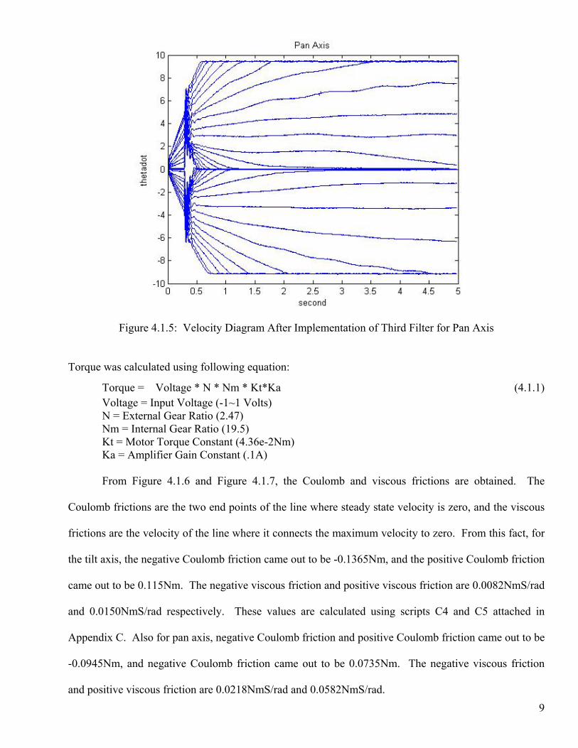
Figure 4.1.5: Velocity Diagram After Implementation of Third Filter for Pan Axis
Torque was calculated using following equation:
Torque = Voltage * N * Nm * Kt*Ka (4.1.1) Voltage = Input Voltage (-1~1 Volts) N = External Gear Ratio (2.47) Nm = Internal Gear Ratio (19.5) Kt = Motor Torque Constant (4.36e-2Nm) Ka = Amplifier Gain Constant (.1A)
From Figure 4.1.6 and Figure 4.1.7, the Coulomb and viscous frictions are obtained. The
Coulomb frictions are the two end points of the line where steady state velocity is zero, and the viscous
frictions are the velocity of the line where it connects the maximum velocity to zero. From this fact, for
the tilt axis, the negative Coulomb friction came out to be -0.1365Nm, and the positive Coulomb friction
came out to be 0.115Nm. The negative viscous friction and positive viscous friction are 0.0082NmS/rad
and 0.0150NmS/rad respectively. These values are calculated using scripts C4 and C5 attached in
Appendix C. Also for pan axis, negative Coulomb friction and positive Coulomb friction came out to be
-0.0945Nm, and negative Coulomb friction came out to be 0.0735Nm. The negative viscous friction
and positive viscous friction are 0.0218NmS/rad and 0.0582NmS/rad. 9
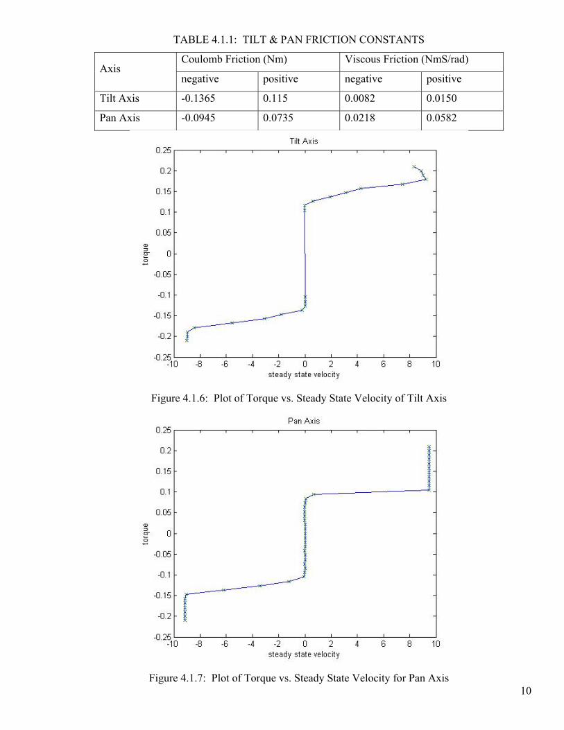
TABLE 4.1.1: TILT & PAN FRICTION CONSTANTS
Coulomb Friction (Nm) Viscous Friction (NmS/rad) Axis
negative positive negative positive
Tilt Axis -0.1365 0.115 0.0082 0.0150
Pan Axis -0.0945 0.0735 0.0218 0.0582
Figure 4.1.6: Plot of Torque vs. Steady State Velocity of Tilt Axis
10Figure 4.1.7: Plot of Torque vs. Steady State Velocity for Pan Axis

Equation (4.1.2) is provided in class lecture notes and the Simulink model in Figure 4.1.8 is
derived from it. Through integration and simplification, matrices are developed in terms of ,θ θ , V,
sample time, and parameter a1, a2, a3, and a4.
(4.1.2) LLL aVaaa θθθθ sin)sgn( 4321 +=++
Figure 4.1.8: Parameter Equation Verifying Simulink Model
A =
⎢⎢⎢⎢⎢
⎣
⎡
∆+−
∆+−
∆+−
− t
t
t
NN )(
)(
)(
221
22
21
21
20
θθ
θθ
θθ
t
t
t
NN ∆+−
∆+−
∆+−
− )(
)(
)(
1
21
10
θθ
θθ
θθ
)(2
)(2)(2
11
121
010
−− −
−−
NNNV
VV
θθ
θθθθ
⎥⎥⎥⎥
⎦
⎤
−−
−−−−
− )cos(cos2
)cos(cos2)cos(cos2
1
12
01
NN θθ
θθθθ
b = a = a = pinv(A)*b
⎥⎥⎥⎥⎥
⎦
⎤
⎢⎢⎢⎢⎢
⎣
⎡
−
−
−
−2
12
21
22
20
21
NN θθ
θθ
θθ
⎥⎥⎥⎥
⎦
⎤
⎢⎢⎢⎢
⎣
⎡
4
3
2
1
aaaa
In order to verify the validity of this method, the parameters, a1, a2, a3, and a4 were set to be
random numbers, 1, 2, 3, and 4 respectively. Data was collected with the chirp input, and the data was
11

again used to calculate parameters using above matrices. a1 was calculated to be 1.0053, a2 came out to
be 1.7730, a3 came out to be 2.8580, and a4 came out to be 4.0053. All four parameters are close to their
original values, proving that the method is valid.
A chirp with frequencies varying from 1 to .1Hz and amplitude of 3 was used as the input
voltage to collect angular displacements and angular velocities of the pan and tilt mechanism. The
resulting output is shown in Figures 4.1.9 and 4.1.10 for the tilt and pan axes respectively. With this
data, the parameters, a1 through a4 were calculated for both pan and tilt axes as shown in Table 4.1.2.
TABLE 4.1.2: PARAMETERS FOR PAN AND TILT AXES
a1 a2 a3 a4
tilt 70.0680 376.8135 783.4932 325 pan 1.7758 4.5490 9.3423 0
Figure 4.1.9: Experimental Data on Tilt Axis with Chirp Input
12

Figure 4.1.10: Experimental Data on Pan Axis with Chirp Input
Now that the parameters are calculated, they have to be checked if they are reasonable on
different types of input voltages. Hence, a sine wave was chosen as the input voltage, and the data
collected from the pan and tilt mechanism. The resulting output for the tilt and pan axes can be seen in
Figures 4.1.11 and 4.1.12.
13

Figure 4.1.11: Experimental Data on Tilt Axis with Sine Input
Figure 4.1.12: Experimental Data on Pan Axis with Sine Input
14

4.2 Control Development
Three gains, derivative, integral, and proportional, are tuned to meet the required transient
response. The proportional gain is tuned for a fast rise time but increases the overshoot. The overshoot
is controlled by derivative gain but also decreases the response time. Finally, the integral gain is tuned
to reduce the steady state error. The objective of the control design was to make the steady state error as
small as possible while maintaining a rapid rise time, with overshoot the least important characteristic.
The gains shown in Table 4.2.1 were found to produce the best response for the model of the system.
These gains are simulated using closed loop feedback as shown in Figure 4.2.1, and the step response for
the tilt and pan axes for the model is that shown in Figures 4.2.2 and 4.2.3 respectively.
TABLE 4.2.1: PID GAINS ON BOTH AXES
kp ki kd
Tilt Axis 50 0.005 0.01 Pan Axis 50 4 10
4pan_theta1
3tilt_theta1
2pan_theta
1ti lt_theta
v oltage_in
v oltage_in1
tilt_theta
pan_theta
Subsystem
Scope1
Scope
In1 Out1
PID 2
In1 Out1
PID 1
1
Gain2
1
Gain1
1
Gain
pan_des
Constant1
tilt_des
Constant
tilt_theta
pan_theta
Figure 4.2.1: Closed Loop Feedback Model
15

Figure 4.2.2: Experimental Data on Tilt Axis with Step Input
Figure 4.2.3: Experimental Data on Pan Axis with Step Input
16
The plots above show that there is some overshoot in the tilt axis, and the response was not too
fast in the pan axis. This response closely matched that of the desired system, with virtually no steady-
state error, relatively small rise times, and a minimal ripple effect.

4.3 Physical Design
To mount the launcher to the pan and tilt mechanism and allow for automated firing requires
substantial modification to the system. First, a way to mount the launcher to a flat surface that could pan
and tilt is necessary. The design in Figure 4.3.1 illustrates the solution to this problem.
Figure 4.3.1: Aluminum Mounting Base
A proper sized piece of aluminum stock can be cut and drilled to specifications. The hole in the
bottom is where the shaft of the tilt axis will slide through and be set-screwed securely on. Once this is
in place, a flat surface perpendicular to the tilt shaft is now available to mount the launcher.
Next, the launcher is reduced to only the components necessary for firing discs. An illustration
of this mechanism can be seen in Figure 4.3.2. By simply connecting the disc spinning motor to a power
source, the launcher can now fire discs as before with less weight, drag, and a now flat and easily
mountable surface.
17

Figure 4.3.2: Disc Launcher
This reduction of the launcher results in removal of the trigger, but this actually aided in the
mounting process. Now, by simply connecting a DC motor to the gear on the bottom of our launcher,
the motor will turn a set distance, turning the gear that pushes the disc into the launching chamber. The
sideways motion at the end of the movement causes the disc to press against the spinning wheel,
propelling it form the launcher. The process is illustrated in Figure 4.3.3. By simply reversing the
voltage on the DC motor for the same set time, the gun can reload as well.
Figure 4.3.3: Automated Firing
18

In order to fit the motor between the base and launcher simple screws, nuts, and washers are all
that is needed. The motor screws into position on the base with the launcher placed above it; the gear on
the motor aligns with the gear on the launcher arm. The launcher is screwed into the base, using the
screws to suspend the launcher in the air while holding it firmly in place; the long screw lengths act as
spacers for the motor. Figure 4.3.4 illustrates the mounting of the launching system.
Figure 4.3.4: Mounting of System
Unfortunately, the automated firing of the disc launcher was not completed as planned. A series
of events occurring within the last few days of the project prevented this idea from becoming a reality.
First, there was a delay in receiving the cable to control the motor via MATLAB and Simulink. Next, it
was found that the motor chosen for the task did not have enough torque to move the launching arm. A
new servomotor was quickly located for replacement, but this motor was found to be too large for the
19

20
already designed and implemented mounting system. With less than a week before the final deadline,
there was not enough time to rebuild the mounting system to accommodate the new motor and then re-
perform all the necessary tests. It was decided to abandon the automatic firing and reloading idea and
simply to launch the discs by manually turning the gear to move the launching arm back and forth. The
original mounting did prove useful for this, allowing room between the base and the launcher to operate
the gear and propel the launching arm. In addition, the mounting was sturdy enough to prevent any
accidental movement in the position or orientation of the launcher when there was human interaction.
4.4 Sensor Development
The impact location sensor being used in the system is a Dynapro 95645 8-wire 13.8” resistive
touchscreen (Appendix B). The screen consists of two sheets of circuit layers separated by a spacer,
with a pliable glass surface on one side and stiff backing on the other. When the glass surface is
touched, there is a voltage change due to the contact of the two circuit layers, which is then sent to a
controller to be decoded into Cartesian coordinates.
The sensor used in the system is a 3M SC801U USB Resistive Controller (Figure 4.4.2). The
controller interfaces directly with the touchscreen and acts as an interpreter between it and a personal
computer. When attached to a personal computer, it behaves as a Human Interface Device, similar to a
mouse [8]. After an impact is registered on the touchscreen, the controller automatically moves the
mouse to the relative position on the computer’s desktop, and sends the command equivalent of a mouse
button click.
Unfortunately, the SC801U is not designed to work with the touchscreen being used, so certain
modifications are required to make it function. The main difficulty lies in the connectors between the
two, specifically that the touchscreen has an XXYY style, non-latched connector pinout, while the
controller expects an XYXY latched connector pinout. X and Y refer to the two sheets in the
touchscreen itself. If the connectors are not mated properly, then the touchscreen acts erratically and the

21
computer receives erroneous data. The pinouts of the controller and touchscreen can be seen in Table
4.4.1.
TABLE 4.4.1: TOUCHSCREEN & CONTROLLER PINOUTS YE- YS- XS+ XE+ YE+ YS+ XS- XE-
Controller 1 2 3 4 5 6 7 8 Touchscreen 1 2 7 8 4 3 6 5
Once a crossover interface is created to correct for the discrepancies between the two connectors,
the controller receives the correct data and is able to interpret it onto the screen. The unavailability of a
USB cable with a Molex 51004-0500 connector to attach to the controller makes the creation of a
custom cable a requirement.
After all of components are successfully integrated, the touchscreen successfully acts as an HID
allowing the input from it to be determined using MATLAB. By superimposing a figure that occupies
the entire screen, it is possible to find the position of the pointer after an impact is detected without
having to worry about the input affecting the computer. After that, it is a simple matter of translating the
pixel location on screen into its appropriate metric translation on the touchscreen, with (0, 0)
representing the center. To accomplish that task, equations (4.4.1) and (4.4.2) are used, where a and b
are the horizontal and vertical screen resolution respectively. The resulting location is the Cartesian
coordinates relative to the touchscreen’s center in millimeters and is passed to the learning algorithm.
x' = (y – b/2) * 206 / b (4.4.1)
y' = (x – a/2) * 279.6 / a (4.4.2)
4.5 Algorithm Development
The Newton-Raphson root finding method is an iterative process that takes, as input, the current
pan and tilt joint angles, as well as the desired x and y positions and the current x and y positions, and
outputs a new set of desired pan and tilt joint angles. The goal is to drive x to xdesired and y to ydesired.
The method can be used if the pan and tilt angles are coupled, however the amount of coupling present

22
due the edges of the touchscreen being farther away from the launcher than the center is minimal and
can be ignored.
The Newton-Raphson equations for the pan angle are simple since the trajectory equation for pan
is the same regardless of the angle of launch and therefore does not have to be scaled to the angle of
firing. The following equations are the calculations for the pan angle and the x directions. Simulation
shows that there is no need to change the alpha constant for the x direction.
X = distance * tan(Qpan) Qpan-new = Qpan – a*(X – Xdesired)/(dX/dQpan) Qpan-new = Qpan – a*(dist*tan(Qpan) – Xdesired)*(cos2(Qpan)) / dist (4.5.1)
For the tilt angle, the equations are a bit more complicated because the trajectory equations have
to be scaled to the angle since the trajectory is differs based on the launcher’s orientation. The
difference shows up in the distance from the y = 0 point on the touchpad that the disc hits. When the
disc is fired downward, it drops more than when it is fired upward due to the aerodynamics. It does not
take as large of a downward angle to yield a given amount of difference in the y direction as it would
take pointing upward to yield the same distance. The equations to get the distance are part of the
advanced trajectory model found in Chapter 5.3. For the learning algorithm, they are incorporated into
the trajectory equations. Table 4.5.1 shows the trajectory equations obtained at various tilt angles. For
the tilt angle, the simulations work well with the alpha constant equal to one so there is no need to
change it.
TABLE 4.5.1: VERTICAL DISPLACEMENT EQUATIONS
Tilt Angle (degrees) Trajectory Equation Used 15 Y=(dist2 + (21.17*dist + 19.2)2)1/2 * (tan(Qtilt)) 10 Y=(dist2 + (13.91*dist + 13.02)2)1/2 * (tan(Qtilt)) 5 Y=(dist2 + (2.8*dist + 2.4)2)1/2 * (tan(Qtilt)) 0 Y=(dist2 + (-.53*dist + .9)2)1/2 * (tan(Qtilt)) -5 Y=(dist2 + (-14.24*dist – 8.94)2)1/2 * (tan(Qtilt)) -10 Y=(dist2 + (-21.88*dist – 13.5)2)1/2 * (tan(Qtilt)) -15 Y=(dist2 + (-37.37*dist – 25.02)2)1/2 * (tan(Qtilt))

23
Since the Newton-Raphson root finding method is robust enough to converge even if the
trajectory equation is not perfect, each equation in the table above is used to satisfy more than one angle.
For example, the 0 degree tilt angle equation is used for any angle between -2.5 degrees and 2.5 degrees;
the 5 degree tilt angle equation is used for any angle from 2.5 degrees to 7.5 degrees, and so forth. In
simulation using MATLAB, this method works well and the proper y position is still found in three tries
so there is no need to obtain more advanced and accurate equations.
The following equations are the Newton-Raphson equations using the trajectory equation for
when the tilt angle is zero.
Qtilt-new = Qtilt – a*(Y – Ydesired)/(dY/dQtilt) Qtilt-new = Qtilt – a*(dist*tan(Qtilt) – Ydesired)*(cos2(Qtilt)) / (dist2 + (-.53*dist + .9)2)1/2 (4.5.2)
With the trajectory equations, it can be predicted where the disk theoretically should hit the
touchpad assuming it follows the equations exactly. In order to filter out unusual launches so that they
are not taken into account by the learning algorithm, the projected point of impact is calculated when the
disk is launched from a given pan and tilt joint angle configuration. The actual point of impact is
compared to the projected point of impact and if there is a difference of more than six centimeters, the
launch is considered inaccurate and is thrown out and another disk is launched. Six centimeters is
thought to be a reasonable value because of the fact that, in the initial testing, most of the disks hit the
touchpad within 4 cm of each other when fired at the same spot. With the launcher being, in general,
accurate to 4 cm, a 6 cm deviation from the projected point of impact is enough to call that specific
launch an unusual case and throw it out.

5. DESIGN VERIFICATION
5.1 Model Verification
Figures 5.1.1 and 5.1.2 show the experimental and simulated angular velocities generated
from a chirp signal input. The experimental angular velocities are filtered to aid in comparison. For
both axes, the system shows both frequencies and amplitudes closely mirroring that of the simulation.
Even though the comparison shows that the parameters are reasonable, another test had to be done. The
parameters are calculated from the experimental data, so it is in a way obvious that the simulated data
should look similar. Therefore, comparing these responses is not enough to determine that the
parameters are accurate. To test the accuracy of the model further, a sine wave is used as an input
instead of a chirp signal, and the resulting responses for the tilt and pan axes can be seen in Figures 5.1.3
and 5.1.4 respectively. Though the results are differ in the first oscillations, which can be attributed to
differences in the starting orientation, the steady state signal are virtually identical.
Figure 5.1.1: Simulation vs. Experimental Response to Chirp Input on Tilt Axis
24

Figure 5.1.2: Simulation vs. Experimental Response to Chirp Input on Pan Axis
Figure 5.1.3: Simulation vs. Experimental Response to Sine Input on Tilt Axis
25

Figure 5.1.4: Simulation vs. Experimental Response to Sine Input on Pan Axis
5.2 Control Verification
In order to verify the transient response meets the specifications, the experimental data is
compared to the angular displacement input to the system. The resulting responses for the tilt and pan
axes are shown in Figure 5.2.1 and 5.2.2, with angular displacements in radians. In the demonstration
and the video clip, it might seem as if there is more overshoot than it is shown in the graph. It is due to
the mounting of the disc launcher, which uses only two supports on the back instead of the four
originally designed. Table 5.2.1 shows the notable aspects of the responses charted. It is to be noticed
that these do not meet the specifications for the pan axis’s rise time or settling time, and the tilt axis’s
settling time or overshoot. Due to the inertia of the system, the tilt axis requires too much proportional
control to expect as low of an overshoot. The pan axis had difficulty meeting the settling time for a
displacement of that magnitude. The specifications were likely overzealous though, as in experimental
work the system responds adequately for the project’s needs. The most important requirement, the
steady-state error, was exceeded by both axes.
26

Figure 5.2.1: Transient Response Due to Step Input on Tilt Axis
Figure 5.2.2: Transient Response Due to Step Input on Pan Axis
TABLE 5.2.1: RESPONSE CHARACTERISTICS OF CLOSED LOOP SYSTEM
Rise Time Steady State Error Settling Time Percent OvershootTilt Axis 0.0230 s 0.8435% 1.21 s 75.1% Pan Axis 0.450 s 0.215% 1.91 s 0.00%
27

In order to check the robustness of the system, the Bode plots of both axes are taken to examine
the gain and phase margins. Figure 5.2.3 shows the tilt axis Bode diagram, while Figure 5.2.4 shows the
pan axis Bode diagram. Table 5.2.2 shows that both axes have an infinite gain margin, as is expected in
the second order system. As such, it does not provide much insight into the stability of the system. The
phase margin of the tilt axis is very large at 170 degrees, so it will not easily be made unstable by a
phase change disturbance. The pan axis is not as stable, with only a 25.7 degree phase margin; however,
that could be remedied in further design refinement by implementing an extra phase-lag compensator on
the pan axis. Doing such should effectively shift the bump in the magnitude high enough so that it only
crosses the 0dB axis once, resulting in a greater phase margin. Regardless, for the design of a prototype
system, a 25.7 degree phase margin is deemed sufficient.
Figure 5.2.3: Tilt Axis Closed Loop Bode Diagram
28

Figure 5.2.4: Pan Axis Closed Loop Bode Diagram
TABLE 5.2.2: GAIN AND PHASE MARGINS OF CLOSED LOOP SYSTEM Gain Margin (dB) Phase Margin (deg)
Tilt Axis Infinity 170 Pan Axis Infinity 25.7
5.3 Physical Verification
To verify that the toy disc shooter obtained is consistent and accurate enough to be viable for use
in the system a several tests are run. The first test is a simple test to determine consistency. Holding the
gun on a level surface and aiming it at a pint glass on the same level surface, the gun was fired 5 times at
a set distance. A diagram of this testing procedure can be seen in Figure 5.3.1.
Figure 5.3.1: Launcher Testing Procedure
29

This sequence is repeated for three trials for each distance. The number of times the disc hit the
glass is recorded and the percent of that number out of 5 is shown in Table 5.3.1. The Total Accuracy of
the disc shooter at that set distance is averaged from the three trials as well.
TABLE 5.3.1: DISC SHOOTER ACCURACY Distance Try 1 Try 2 Try 3 Total Accuracy
3ft 0.9m 100% 100% 100% 100%
5ft 1.5m 80% 100% 100% 93.33%
7ft 2.1m 80% 80% 80% 80%
9ft 2.75m 80% 60% 80% 73.33%
11ft 3.35m 80% 100% 80% 86.67%
13ft 4m 60% 60% 40% 53%
Finding the results of this first experiment satisfactory, it is decided that the disc shooter can be
used. To obtain a more accurate understanding of how the disc is fired and how it travels a second test
was designed to determine the trajectory of the disc after being launched from the toy gun. This
experiment is set up similarly to the previous one. The gun is held on a level surface and now aimed at a
piece of paper with a graph drawn on it. This graph has marks for each centimeter vertically and
horizontally away from the origin and is taped to the wall so that the origin is on the same level surface
as that of the barrel of the toy gun. This experiment is illustrated in figure 5.3.2.
Figure 5.3.2: 2nd Launcher Testing Procedure
30

31
The gun is fired 10 times at a set distance and the x and y coordinates where the disc hit are
recorded for each shot. The gun is then moved to another set distance and the experiment repeated. The
results of this experiment are listed in Table 5.3.2.
TABLE 5.3.2: PRELIMINARY TRAJECTORY RESULTS 0.5 m 1.0 m 1.5 m 2.0m
Shot #
x position in cm from origin
y position in cm from origin
x position in cm from origin
y position in cm from origin
x position in cm from origin
y position in cm from origin
x position in cm from origin
y position in cm from origin
1 -2 -1 0 -6 0 -10 X X 2 -2 -1 0 -3 -1 -11 X X 3 0 -1 1 -5 5 -9 X X 4 -2 -2 -3 -5 2 -11 X X 5 -1 -2 1 -5 1 -9 X X 6 1 -1 -2 -5 -1 -10 X X 7 -1 0 -3 -5 -1 -10 -1 -13 8 -2 0 2 -4 2 -9 X X 9 -2 0 0 -6 -2 -11 X X 10 0 0 -2 -5 -2 -11 X X
• X means the disc hit lower than -14cm and could not be recorded
The conclusion drawn from this experiment is that the trajectory should be determined from data
collected between 0.5 and 1.5 meters. Anything before 0.5 meters will be fired at a negative angle and
anything after 1.5 meters will be fired at a positive angle relative to the horizon. This led to the next
experiment that is performed in the exact same matter as above. The result of the trajectory experiment
with data from 0.5 to 1.5 meters is shown in Table 5.3.3. The experiment is graphed in Figure 5.3.3.
TABLE 5.3.3: SHORT RANGE TRAJECTORY RESULTS
Shot #
0.5 m (x
position in cm from
origin)
0.5 m (y
position in cm from
origin)
0.7 m (x
position in cm from
origin)
0.7 m (y
position in cm from
origin)
0.9 m (x
position in cm from
origin)
0.9 m (y
position in cm from
origin) 1 -2 -1 1 -2 0 -4 2 -2 -1 0 -2 2 -3 3 0 -1 2 -2 -1 -5 4 -2 -2 -2 -2 -2 -4 5 -1 -2 4 -1 0 -3 6 1 -1 3 -2 -1 -4 7 -1 0 -2 -1 -1 -5 8 -2 0 -2 -1 1 -3 9 -2 0 -1 -2 3 -2
10 0 0 3 0 0 -2

1.0 m (x position in cm from
origin)
1.0 m (y position in cm from
origin)
1.1 m (x position in cm from
origin)
1.1 m (y position in cm from
origin)
1.3 m (x position in cm from
origin)
1.3 m (y position in cm from
origin)
1.5 m (x position in cm from
origin)
1.5 m (y position in cm from
origin) 0 -6 0 -5 0 -6 0 -10 0 -3 -2 -6 -1 -7 -1 -11 1 -5 -1 -6 -5 -6 5 -9 -3 -5 -2 -8 -3 -10 2 -11 1 -5 0 -5 -5 -10 1 -9 -2 -5 0 -6 1 -5 -1 -10 -3 -5 0 -6 2 -6 -1 -10 2 -4 -1 -8 0 -8 2 -9 0 -6 2 -7 2 -5 -2 -11 -2 -5 -2 -7 -2 -9 -2 -11
Position of each individual trial disc at target from given distance
-12
-10
-8
-6
-4
-2
0
2
4
-6 -4 -2 0 2 4 6
x-position (cm)
y-po
sitio
n (c
m)
From 0.5 metersFrom 0.7 metersFrom 0.9 metersFrom 1.0 metersFrom 1.1 metersFrom 1.3 metersFrom 1.5 meters
Figure 5.3.3: Plot of Short Range Trajectory Results
A summary of this experiment can be seen in the Table 5.3.4, which shows the average x and y
displacement at each distance in centimeters.
TABLE 5.3.4: AVERAGE SHORT RANGE TRAJECTORY 0.5 m (x position)
0.5 m (y position)
0.7 m (x position)
0.7 m (y position)
0.9 m (x position)
0.9 m (y position)
-1.1 -0.8 0.6 -1.5 0.1 -3.5
1.0 m (x position)
1.0 m (y position)
1.1 m (x position)
1.1 m (y position)
1.3 m (x position)
1.3 m (y position)
1.5 m (x position)
1.5 m (y position)
-0.6 -4.9 -0.6 -6.4 -1.1 -7.2 0.3 -10.1 32

From this data, it can be concluded that the horizontal displacement of the disc stays relatively
close to zero with a maximum of 1 cm average deviation from the origin. It can also be seen that as the
distance from the target increases, the vertical position that the disc strikes the target also decreases. A
plot of distance from target (in meters) vs. vertical position relative to the horizontal (in centimeters) is
shown in Figure 5.3.4.
Average Vertical Displacement vs. Distance from launcher to target
-12
-10
-8
-6
-4
-2
0
2
4
0.5 0.7 0.9 1 1.1 1.3 1.5
Distance from launcher to target (meters)
Aver
age
Verti
cal D
ispl
acem
ent (
cm)
AverageStandard Deviation
Figure 5.3.4: Average Vertical Displacement vs. Distance from Launcher to Target
Fitting a best-fit line to this data, the equation is found to be Y = -9.5X + 4.59, where X is the
distance from the gun barrel to the target and Y would be the vertical displacement where the disc would
hit the target. This equation is a good estimation of the trajectory of the disc knowing the distance to the
target between 0.5 and 1.5 meters. This equation can be used to estimate the vertical position at which
the disc will strike the target if the distance from the launcher barrel to the target is known. This
equation can also be used to estimate the distance the launcher is from the target given the vertical
displacement of the striking area of the disc. A final use for this equation comes into the learning
algorithm where knowing both the distance from the launcher to the target and the vertical displacement
33

34
of the disc at the target, the algorithm can check the accuracy of the shot by comparing it with this
model.
In an effort to create the most accurate trajectory model for the disc launched from the toy gun a
third and final test is established. This experiment is again set up similarly to the previous two trajectory
tests, with the launcher being held securely to the mount attached to the pan and tilt mechanism for more
stability. The gun was once again aimed at a graph with one centimeter scaling for the horizontal and
vertical deviations from the origin that was lined up with the mouth of the launcher. Again, see Figure
5.3.2.
This test continued in similar fashion as before with ten shots being fired at each set distance
from the launcher to the graph, and at each of seven angles at that set distance. The set distances were
0.5, 0.75, 1.0, 1.25, and 1.5 meters and the set angles were -15°, -10°, -5°, 0°, 5°, 10°, and 15° from the
horizon. These are chosen based on previously defined requirements and experimentation.
Since it was determined from the previous experiment (and continually shown throughout this
one) that the x direction had little deviation, only the y coordinate where the disc struck the graph was
recorded. Once again, it was attempted to get best fit lines from this data to determine the trajectory of
the disc given the distance from the launcher to the target. The average vertical displacement of the 10
shots at each set angle at each set distance is shown in Table 5.3.5. The X’s in the table mean that the
disc hit the ground before the target.
TABLE 5.3.5: AVERAGE VERTICAL DISPLACEMENT AT SET ANGLE AND DISTANCE Distance 0.5 0.75 1 1.25 1.5 15 18.8 20.2 25.2 25.5 26 10 10.3 15.7 17.5 15.8 14.7 5 2.6 2.5 3.3 3.5 4.1 Angle 0 0 -0.3 -1 -2.4 -6.1 -5 -9.1 -13.4 -20.5 -24.8 -29.9 -10 -15 -19.3 -30.8 -39.3 -46.9 -15 -25.1 -37.2 -49.8 X X
From this data, a line was graphed for each angle so that a best fit line could be determined in the
form of Y=aX+b where X is a known distance from the launcher to the target and Y is the vertical

displacement, or the position the disc should hit the target based on the angle that the launcher is
currently firing at. A graph of these lines can be seen in Figure 5.3.5.
Y position vs X distance from target at each set angle
-60
-50
-40
-30
-20
-10
0
10
20
30
0.5 0.75 1 1.25 1.5
Distance from launcher to target
verti
cal d
ispl
acem
ent 15 degrees
10 degrees5 degrees0 degress-5 degrees-10 degrees-15 degrees
Figure 5.3.5: Graph of Y Position vs. X Distance from Target at Each Set Angle
This leads to the advanced trajectory model used in the learning algorithm. The equations for the
best fit lines at each angle are displayed in Table 5.3.6.
TABLE 5.3.6: VARIABLES A & B IN Y = AX + B BEST FIT LINE EQUATIONS Angle a b
15° 19.2 21.1710° 13.02 13.91
5° 2.4 2.80° 0.9 -0.53
-5° -8.94 -14.24-10° -13.5 -21.88-15° -25.0167 -37.3667
These equations are fed into the learning algorithm, which uses them to compute the new
position and orientation of the launcher based on the distance from the launcher to the target, and the
current angle of the firing mechanism.
The size of the target will dictate the required accuracy for the system. The initial expectation is
that the firing system be able to hit consistently within a 7.5 cm diameter circle at a maximum range of
1.5m, when at a zero degree tilt. Through simple trigonometry, it can be deduced that ensuring an 35

impact within 3.25 cm of center at 1.5 m requires that the rotational position be within ±1.24 degrees.
Taking into account the standard deviation of the horizontal displacements shown in Table 5.3.3 and
Figure 5.3.4, the largest standard deviation was 2.60 cm, with the deviation at 1.5m being 2.21 cm. By
subtracting the standard deviation from the allowable error, a circle of approximately 1 cm radius is left,
resulting in a maximum position error of ±0.382 degrees. The specified error of ±0.1 degrees falls well
within the tolerable error, and should allow the desired target to be hit at an even greater range with
consistency. The mechanism itself should have no difficulty achieving this low error, as the encoder
allows for accuracy within 0.0439 degrees since it has a 2048-bit quadrature reading on the output shaft.
Figure 5.3.6 shows the offset resulting from the possible position errors discussed above. Since the
current trajectory of vertical motion is a best-fit line, it can be assumed that the same values will hold
true for the tilt axis. These are likely to differ once a more precise trajectory can be calculated
experimentally; however, it appears that a ±0.1 degree error will supply the necessary accuracy and
feasibility for the project.
0 0.5 1 1.5-0.04
-0.03
-0.02
-0.01
0
0.01
0.02
0.03
0.04
X: 1.5Y: 0.01
X: 1.5Y: -0.002618
X: 1.5Y: -0.03246
Target ConeTarget ConeAllowable ErrorAllowable ErrorDesired ErrorDesired Error
Figure 5.3.6: Target Cones Resulting from Different Position Errors
365.4 Sensor Verification

Since the most important part of the system is accuracy, it is critical that the sensor used to detect
impacts be as precise as possible. As shown in Figure 5.4.1, the touchscreen itself has a dot pitch of 160
mil, which is more than accurate enough to give the location of the size disc being used. The limiting
factor then becomes the controller itself, as it has only the ability to transmit 10-bit coordinate data [8].
That allows for a vertical resolution of 0.27 mm and horizontal resolution of 0.20 mm. Even with the
lower resolution, it is more than capable of accurately sensing the location of impact.
Figure 5.4.1: Dot Pitch of Touchscreen Sensor
Once the accuracy of the touchscreen itself is established, the consistency between the
touchscreen input and output on the computer must be verified. In testing each corner of the screen, it
can be seen that the pointer reaches the bottom corners of the screen perfectly, while falling a few pixels
short of the top corners. That discrepancy is likely due to the high resolution of the monitor used
relative to the controllers, combined with the small dead zones at the corners of the touchscreen.
Fortunately, the dead zone was found to be only six pixels wide, or approximately 0.57% of the screen.
Considering the likelihood of the disc striking precisely the corner of the touchscreen without activating
one of the nearby sensors, it can be safely assumed that the dead zone will not significantly alter the
results of the system. Random test points throughout the monitor confirmed that the calibration of the
touchscreen is accurate enough to ensure proper reading of the results.
37

38
The problem with the touchscreen comes when discs are fired at it. Although able to respond to
the slightly prick of a fingertip, the disc is unable to activate the sensor. Several factors thought to play
a part in the sensor’s failure can be tested. The mass of the disc is minute, and even though it is fired at
high velocities, it is possible that the momentum is insufficient to bend the screen enough to connect the
two circuit sheets. The problem is not as simplistic as using a heavier mass, as attempts to activate the
sensor using a mouse ball thrown at high speeds fail as well. The possibility that organic contact is
required to activate the sensor can be dismissed as pressing any object against the screen succeeding in
activating it. The conclusion that contact with the screen must be prolonged for a longer period of time
than an elastic collision permits in order to register an impact is the only remaining conclusion. Having
no means to accomplish this task or time to pursue other sensory options when this difficulty was
encountered, the location of the impact is now manually entered on the touchscreen.
In experimentation, the touchscreen did provide accurate feedback to the learning algorithm
when the impact location was manually input. The launcher converged on the target in three shots, and
thus from that aspect the sensor can be considered a success. It is likely in further refinement that it will
be replaced by one more capable of detecting rapid and faint impacts however.
5.5 Algorithm Verification
In order to verify that the Newton-Raphson root finding method is a suitable learning algorithm,
it has to be simulated on MATLAB. A script is written for this purpose. The following figure displays
the simulation for the pan angle. The desired x position is at x = 20 and the starting x position is at zero,
with an angle of zero degrees. It is assumed that the first launch hits the touchpad at zero. It can be seen
from the figure that it converges at x = 20 within three tries.

0 1 2 3 4 5 6 7 8 9 100
5
10
15
20
25Newton-Raphson Simulation for Pan Angle: Xdesired = 20 cm
X p
ositi
on
iteration
Figure 5.5.1: Simulated Newton-Raphson Pan Angle Algorithm Results
In reality, it also only took three tries to hit the target on most runs. However, they do not
converge quite as neatly in the actual running of the system. Although it hits the target in three tries, it
does not hit the center of the target or get as close to the target on the second try as when simulated. The
cause for the discrepancy is the launcher’s lack of perfect repeatability. Fortunately, the learning
algorithm is robust enough that it can still converge on the target even if the trajectory is a little off.
For the tilt trajectory, the results are similar. The ideal simulation converges on the target within
three tries. The numbers in the idea simulation are slightly different in that the second try is farther
away from y = 20 than it was for the x simulation but that is because the trajectory equations are
different for the tilt angle. The fact that the tilt angle also converges in three tries proves that the
algorithm will still converge on the desired location even if the trajectory is not perfect. The tilt axis
trajectories were done such that each trajectory was used for a small range of angles so it is not as
precise as the pan axis. The algorithm still converges, so the fact that the trajectory in the y direction is
imperfect does not significantly affect the results. Figure 5.5.2 shows the simulation results when the
learning algorithm is tested in MATLAB for the tilt angle.
39

0 1 2 3 4 5 6 7 8 9 100
5
10
15
20
25Newton-Raphson Simulation for Tilt Angle: Ydesired = 20 cm
Iteration
Y P
ositi
on
Figure 5.5.2: Newton-Raphson Tilt Angle Algorithm Results
In reality, when the algorithm is tested with the actual pan and tilt device, the tilt angle is not
quite as accurate as the pan angle. This is probably because the launcher is more unpredictable in the y
direction than it is in the x direction as was seen in the initial launcher test results. It was found that in
the y direction sometimes the launcher did not move as much as it should have.
Another factor in the performance of the algorithm is the filtration of outlying impacts from
being used in calculation. The performance of the learning algorithm in the tilt direction can probably
be improved if the tolerance is lowered to four or five centimeters because then more shots would be
thrown out as unusual cases. A deviation from the projected point of more then four centimeters is more
common in the y direction then in the x direction.
40

41
6. COSTS
The cost of the assembled pan and tilt system used as the basis of this project has been itemized
and calculated as follows in Table 6.1.
TABLE 6.1: PAN AND TILT MECHANISM COST Item
Part Number Price ($) Quantity Total ($)
Motor
GM8724S017 192.86 [1] 2 385.72
Timing Belt
A6Z16-C01806 1.86 [1] 2 2.70
Encoder
S1 & S2 Optical Shaft Encoders
49.00 [3] 2 98.00
Gear
A6A6-75NF01812 A6A6-25DF01806
15.15 [1] 7.76 [1]
2 2
30.30 15.52
Total 532.24
The costs of additional parts and programs needed for the complete system beyond those of the
assembled pan and tilt mechanism are listed in Table 6.2.
TABLE 6.2: COST OF ADDITIONAL PARTS NEEDED FOR SYSTEM
Item
Price ($) Quantity Total
Toy Disc Shooter and Discs
4.97 2 9.94
Touchpad Touchpad Controller
24.95 [4] 50.00
1 24.95 50.00
Wires (spool)
4.00 1 4.00
Programs: SolidWorks MATLAB 7 Simulink 6
64.98 [7] 1900.00[2]2800.00[7]
1 4 4
64.98 7,600.00 11,200.00
Motor [6] Gears [6]
3.00 2.25
1 1
3.00 2.25
Clamps (for Mounting)
8.95 1 8.95
TOTAL
18,968.07

42
The labor cost of designing, building, testing and operating the system among the four members
of the group are listed in Table 6.3.
TABLE 6.3: LABOR COSTS Laborer Salary ($/hr) Hours/Week Weeks Total ($) Ryan Kindle
25 10 10 2,500
Diana Mirabello
25 10 10 2,500
Yena Park
25 10 10 2,500
Josh Schuster
25 10 10 2,500
Total for 4 Employees ($)
10,000
The use of different labs to build and test the system has been assumed to cost as follows in
Table 6.4 and the total system costs are listed in Table 6.5.
TABLE 6.4: LAB USAGE COSTS Lab Rate ($/day) Use (days) Total ($) Control Systems Lab
50 30 3,000
Engineering Lab
50 4 200
Total 3,200
TABLE 6.5: TOTAL SYSTEM COSTS Pan and Tilt Mechanism
Additional Parts Needed for System
Labor Costs
Lab Use
Total
$532.24
$18,968.07 $10,000 $3,200 $32,700.31
Seeing as many of the components, programs, labs and equipment are provided free of charge,
along with the fact that there is no labor cost, the actual cost to the group can be calculated and is
displayed in Table 6.6.
TABLE 6.6: ACTUAL COST OF SYSTEM Pan and Tilt Mechanism
Additional Parts Needed for System
Labor Costs
Lab Use
Total
$0
$97.04 $0 $0 $99.09

43
7. CONCLUSIONS
Despite some setbacks, the system was an overall success and many of the goals put forth in the
project proposal were achieved. In the end, the working system was able to fire discs at a target on a
touchscreen and then correct for error using an iterative learning algorithm, usually converging on the
target in three tries. The only major problems that prevented some of the original goals from being met
were problems with equipment that prevented the system from having automated firing and feedback.
The controllers designed for both the pan and the tilt angles worked very well. They moved
quickly to the proper pan and tilt joint angles with negligible steady-state error. There was a slight
amount of overshoot, however that was not a concern for this project since the final position of the
launcher was more important that its trajectory.
The learning algorithm worked very well in the pan direction and performed similarly to the
initial MATLAB simulation. In the pan direction, it could converge on the target within three tries
almost every time. In the tilt direction, the learning algorithm worked well after some tuning of the
alpha constant since at first it converged significantly slower then it had in the initial simulation. In the
end, the system was able to converge on the target in three tries almost every time, with both the pan and
the tilt directions working correctly.
Unfortunately, automated firing of the launcher was not completed. This was due to the
difficulty in getting the servomotor to work, and the DC motor’s insufficient torque. Given more time to
either find a motor with more torque, or adjust the mounting to allow for the integration of the
servomotor, automated firing could be accomplished. The servomotor provided did seem to have a slow
reset time however, upwards of twenty seconds, so it would not be ideal for this application and further
investigation into other methods might prove useful.
The system was supposed to get automatic feedback from the touchscreen when the disc hit it,
and its failure was another major setback. Though the touchscreen was very accurate in detecting
position, it could not detect the discs being fired at it because they did not make contact with the

44
touchscreen for a long enough amount of time to register. Instead, the impact location had to be
manually entered on the touchscreen to provide the feedback required. Once that was done however, it
was able to send the data to the computer with no problems whatsoever.
Though a completely automated system would have been ideal, the results of the prototype are
quite promising overall since the control portions of the system all worked well. Given time for further
refinement and development, automated firing could have been accomplished and alternate sensor
options explored. Extensions to the system developed include the installation of a directional sensor so
that the launcher can detect the approximate location of the target without manual aiming, and the
application of the system to other kinds of projectile launchers.

45
8. REFERENCES
[1] Bowen, Luke, Cieloszyk, Matt and Gillette, Rob. “Team 5 Proposal.” Team 5 Proposal. 2/22/2004. http://www.cat.rpi.edu/~wen/ECSE4962S04/proposal/team5proposal.pdf [2] Strassberg, Dan. “Math, simulation updates offer new programming tools, faster development.” EDN.com. 6/10/2004. http://www.edn.com/article/CA421495.html [3] Wen, John. “S1 & S2 Optical Shaft Encoders.” Encoder Datasheet. 9/26/02. http://www.cat.rpi.edu/~wen/ECSE4962S03/encoder_datasheet.pdf [4] “Action Solutions.” Action Solutions. 2004. http://www.actionsolutions.com/subcat.asp?departmentid=74 [5] “High Power Infrared LEDs.” Reynolds Electronics. 2000. http://www.rentron.com/Products/Electronic-Components.htm [6] “Motors, Servos, Wheels and H-Bridges Section.” Hobby Engineering. 2/28/2005. http://www.hobbyengineering.com/SectionM.html [7] “SolidWorks Student Edition 2004-2005.” JourneyEd.com. 2004. http://www.journeyed.com/itemDetail.asp?GEN0=01&GEN1=01&GEN2=SOLI DWORKS&GEN3=JEM&T1=36785643FS6 [8] “SC800 USB Resistive Controller Reference Guide.” 3m.com. 2004. http://www.3m.com/3MTouchSystems/downloads/PDFs/19-273.pdf

46
Appendix A: Contribution of Team Members
Ryan Kindle ________________________ • Introduction / Professional & Societal Considerations • Sensor Development • Sensor Verification • Control Verification • Editing & Compilation
Diana Mirabello ________________________
• Friction Identification • Algorithm Development • Algorithm Verification • Conclusion
Yena Park ________________________
• Friction Identification • Model Development • Model Verification • Control Development • Control Verification
Josh Schuster ________________________
• Physical Development • Physical Verification • Control Verification • Costs

Appendix B: Datasheets
47

48

49 49

50
Appendix C: MATLAB Scripts
Script C1: %%%%%%%%%%%%%%%%%%%%%%%%%%%%%%%%%%%%%%%%%%% %friction_param_save_tilt.m %02/26/05 %run friction_param.mdl in a for loop %collect the data and plot it %%%%%%%%%%%%%%%%%%%%%%%%%%%%%%%%%%%%%%%%%%% voltage_range = [-1:.05:1]; times = [0:0.001:5]; for k = 1:length(voltage_range) voltage_range(k) for i = 1 : 5 setparam(tg, 28, voltage_range(k)); i if voltage_range(k)==0 else if voltage_range(k)>0 setparam(tg, 27, 10); setparam(tg, 24, 10); else setparam(tg, 27, -10); setparam(tg, 24, -10); end start(tg); pause(5); stop(tg); outputlog = tg.OutputLog; theta_1(i, :) = outputlog(:, 1); theta_dot_1(i, :) = outputlog(:, 2); voltage_out(i, :) = outputlog(:, 5); pause(.5); end end %first filtering thetadot_ave_temp(k, :) = (theta_dot_1(1, :)+theta_dot_1(2, :)+theta_dot_1(3, :)+theta_dot_1(4, :)
+theta_dot_1(5, :))/5; %second filtering for j = 1 : length(thetadot_ave_temp(k, :)) - 25 sum = 0; for ii = 0 : 24 sum = sum + thetadot_ave_temp(k, j+ii); end thetadot_ave(k,j) = sum/25;

51
end end %third filtering for i = 1 : 41 for j = 1 : 4975 if abs(thetadot_ave(i, j) - thetadot_ave(i, j+1))>1 thetadot_ave(i, j +1) = (thetadot_ave(i, j) + thetadot_ave(i, j + 2))/2; end end end for i = 1 : 25 plot(times(1:4976), thetadot_ave(i, :)); hold on; end ylabel('thetadot'); xlabel('second'); title('Tilt Axis'); save tilt_axis.mat thetadot_ave_temp thetadot_ave

52
Script C2: %%%%%%%%%%%%%%%%%%%%%%%%%%%%%%%%%%%%%%%%%%% %friction_param_save_pan.m %02/26/05 %run friction_param.mdl in a for loop %collect the data and plot it %%%%%%%%%%%%%%%%%%%%%%%%%%%%%%%%%%%%%%%%%%% % voltage_range = [-1, -.95, -.9, -.85, -.8, -.75, -.7, -.65, -.6, -.55, -.5 .5, .55, .6, .65, .7, .75, .8, .85, .9, .95, 1]; voltage_range = [-.45:.05:.45]; %[.1:.1:.1]; for k = 1:length(voltage_range) voltage_range(k) for i = 1 : 5 times = [0:0.001:5]; setparam(tg, 29, voltage_range(k)); i if voltage_range(k)==0 else if voltage_range(k)>0 setparam(tg, 28, 10); setparam(tg, 25, 10); else setparam(tg, 28, -10); setparam(tg, 25, -10); end start(tg); pause(5); stop(tg); outputlog = tg.OutputLog; theta_1(i, :) = outputlog(:, 3); theta_dot_1(i, :) = outputlog(:, 4); voltage_out(i, :) = outputlog(:, 5); pause(.5); end end % [num, den] = butter(10, 0.005); % butter_filter = tf(num,den, 0.001); % thetadot1(i,:) = lsim(butter_filter, theta_dot_1(i, :), times); % thetadot1_butter(i, :) = theta_dot_1(i, :).* butter_filter; thetadot1_ave1(k, :) = (theta_dot_1(1, :)+theta_dot_1(2, :)+theta_dot_1(3, :)+theta_dot_1(4, :)
+theta_dot_1(5, :))/5; for j = 1 : length(thetadot1_ave1(k, :)) - 25 sum = 0; for ii = 0 : 24

53
sum = sum + thetadot1_ave1(k, j+ii); end thetadot1_ave2(k,j) = sum/25; end end for i = 1 : length(thetadot1_ave2) plot(times(1:4976), thetadot1_ave2(i, :)); hold on; end

54
Script C3: %%%%%%%%%%%%%%%%%%%%%%%%%%%%%%%%%%%%%%%%%%%%%%% %02/26/05 %set the initial values for friction_param.mdl %put the logs on the signals %subsystem under friction_param.mdl needs to be selected before running %this file %%%%%%%%%%%%%%%%%%%%%%%%%%%%%%%%%%%%%%%%%%%%%%% ts = 0.001; %sample time const_voltage = 666; peak_voltage =777; handles = get_param(gcb, 'porthandles'); outputports = handles.Outport; for i = 1 :length(outputports) set_param(outputports(i), 'DataLogging', 'on'); set_param(outputports(i), 'TestPoint', 'on'); end set_param(outputports(1), 'Name', 'theta1_log'); set_param(outputports(2), 'Name', 'thetadot1_log'); set_param(outputports(3), 'Name', 'theta2_log'); set_param(outputports(4), 'Name', 'thetadot2_log'); set_param(outputports(5), 'Name', 'voltage_log');

55
Script C4: %%%%%%%%%%%%%%%%%%%%%%%%%%%%%%%%%%%%%%%%%%%%%%%%%% %steady_state_tilt.m %2/26/05 %By Yena Park %%%%%%%%%%%%%%%%%%%%%%%%%%%%%%%%%%%%%%%%%%%%%%%%%% clear save_torque close all clear all % voltage = [-1:.05:1]; load datalog.mat voltage = [-1, -.95, -.9, -.85, -.8, -.75, -.7, -.65, -.6, -.55, -.5, .5, .55, .6, .65, .7, .75, .8, .85, .9, .95, 1]; %calculate Torque N1 = 2.47; %External Gear Ratio Nm1 = 19.5; %Internal Gear Ratio Kt = 4.36e-2; %motor torque constant Ka = .1; %amplifier gain constant torque = voltage .* N1 * Nm1 * Kt * Ka; k = 1; positive = 0; viscous_friction_negative_sum = 0; viscous_friction_positive_sum = 0; negative_count = 0; positive_count = 0; for i = 1 : 22 thetadot1_ss(i) = 0; for j = 4976-1000:4976 thetadot1_ss(i) = thetadot1_ss(i) + thetadot1_ave2(i, j)/1000; end if abs(thetadot1_ss(i)) < 0.0001 save_torque(k) = torque(i); k = k + 1; positive = 1; elseif i ~= 1 && abs(thetadot1_ss(i) - thetadot1_ss(i-1))>0.05 if positive ==0 viscous_friction_negative_sum = viscous_friction_negative_sum + (torque(i)-torque(i-1))
/(thetadot1_ss(i)-thetadot1_ss(i-1)); negative_count = negative_count + 1; else viscous_friction_positive_sum = viscous_friction_positive_sum + (torque(i)-torque(i-1))
/(thetadot1_ss(i)-thetadot1_ss(i-1)); positive_count = positive_count + 1; end end end coulomb_friction_negative_tilt = save_torque(1) coulomb_friction_positive_tilt = save_torque(k-1)

56
viscous_friction_negative_tilt = viscous_friction_negative_sum/negative_count viscous_friction_positive_tilt = viscous_friction_positive_sum/positive_count plot(thetadot1_ss, torque, thetadot1_ss, torque, 'x') xlabel('steady state velocity') ylabel('torque'); title('Tilt Axis');

57
Script C5: %%%%%%%%%%%%%%%%%%%%%%%%%%%%%%%%%%%%%%%%%%%%%%%%%% %steady_state_pan.m %2/26/05 %By Yena Park %%%%%%%%%%%%%%%%%%%%%%%%%%%%%%%%%%%%%%%%%%%%%%%%%% voltage = [-1:.05:1]; %calculate Torque N1 = 2.47; %External Gear Ratio Nm1 = 19.5; %Internal Gear Ratio Kt = 4.36e-2; %motor torque constant Ka = .1; %amplifier gain constant torque = voltage .* N1 * Nm1 * Kt * Ka; k = 1; positive = 0; viscous_friction_negative_sum = 0; viscous_friction_positive_sum = 0; negative_count = 0; positive_count = 0; for i = 1 : 41 thetadot2_ss(i) = 0; for j = 4976-1000:4976 thetadot2_ss(i) = thetadot2_ss(i) + thetadot2(i, j)/1000; end if abs(thetadot2_ss(i)) < 0.0001 save_torque(k) = torque(i); k = k + 1; positive = 1; elseif i ~= 1 && abs(thetadot2_ss(i) - thetadot2_ss(i-1))>0.05 if positive ==0 viscous_friction_negative_sum = viscous_friction_negative_sum + (torque(i)-torque(i-1))
/(thetadot2_ss(i)-thetadot2_ss(i-1)); negative_count = negative_count + 1; else viscous_friction_positive_sum = viscous_friction_positive_sum + (torque(i)-torque(i-1))
/(thetadot2_ss(i)-thetadot2_ss(i-1)); positive_count = positive_count + 1; end end end coulomb_friction_negative_pan = save_torque(1) coulomb_friction_positive_pan = save_torque(k-1) viscous_friction_negative_pan = viscous_friction_negative_sum/negative_count viscous_friction_positive_pan = viscous_friction_positive_sum/positive_count plot(thetadot2_ss, torque, thetadot2_ss, torque, 'x') xlabel('steady state velocity') ylabel('torque'); title('Pan Axis');

58
Script C6: %%%%%%%%%%%%%%%%%%%%%%%%%%%%%%%%%%%%%%%%%%%%%%%%%%%%%%%%%%%%%%%%%%%%%%%%%%% %param_calc_tilt.m %3/26/05 %By Yena Park %%%%%%%%%%%%%%%%%%%%%%%%%%%%%%%%%%%%%%%%%%%%%%%%%%%%%%%%%%%%%%%%%%%%%%%%%%% clear A b col1 col2 col3 col4 ts = 0.001; for i = 1 : length(theta1_ave)-1 col1 = -(thetadot1_ave(i)^2 + thetadot1_ave(i+1)^2)*ts; col2 = -(abs(thetadot1_ave(i)) + abs(thetadot1_ave(i+1)))*ts; col3 = 2 * voltage_in(i) *(theta1_ave(i+1) - theta1_ave(i)); col4 = -2*(cos(theta1_ave(i+1)) - cos(theta1_ave(i))); A(i, :) = [col1 col2 col3 col4]; b(i) = thetadot1_ave(i+1)^2 - thetadot1_ave(i)^2; end a_tilt = pinv(A)*b' Script C7: %%%%%%%%%%%%%%%%%%%%%%%%%%%%%%%%%%%%%%%%%%%%%%%%%%%%%%%%%%%%%%%%%%%%%%%%%%% %param_save_pan.m %3/26/05 %By Yena Park %%%%%%%%%%%%%%%%%%%%%%%%%%%%%%%%%%%%%%%%%%%%%%%%%%%%%%%%%%%%%%%%%%%%%%%%%%% ts = 0.001; clear A b col1 col2 col3 col4 for i = 1 : length(thetadot_ave)-1 col1 = -(thetadot_ave(i)^2 + thetadot_ave(i+1)^2)*ts; col2 = -(abs(thetadot_ave(i)) + abs(thetadot_ave(i+1)))*ts; col3 = 2 * voltage_in(i) *(theta2_ave(i+1) - theta2_ave(i)); col4 = -2*(cos(theta2_ave(i+1)) - cos(theta2_ave(i))); A(i, :) = [col1 col2 col3 col4]; b(i) = thetadot_ave(i+1)^2 - thetadot_ave(i)^2; end a_pan = pinv(A)*b'

59
Script C8: %%%%%%%%%%%%%%%%%%%%%%%%%%%%%%%%%%%%%%%%%%%%%%%%%% %param_save_pan.m %3/25/05 %By Yena Park %%%%%%%%%%%%%%%%%%%%%%%%%%%%%%%%%%%%%%%%%%%%%%%%%% clear theta2 thetadot2 voltage_in voltage_in_sum theta2_sum thetadot2_sum voltage_in_ave theta2_ave thetadot2_ave times = [0:0.001:14]; for k = 1:1 start(tg); pause(14); stop(tg); outputlog = tg.OutputLog; theta2(k,:) = outputlog(:, 3); thetadot2(k, :) = outputlog(:, 4); voltage_in(k, :) = outputlog(:, 5); pause(0.5); end % voltage_in_sum(1:14285) = 0; % theta2_sum(1:14285) = 0; % thetadot2_sum(1:14285) = 0; % % for i = 1 : 10 % voltage_in_sum = voltage_in_sum + voltage_in(i, :); % theta2_sum = theta2_sum + theta2(i, :); % thetadot2_sum = thetadot2_sum + thetadot2(i,:); % end voltage_in_ave = voltage_in; theta2_ave = theta2; thetadot2_ave = thetadot2; j = 1; for i = 1 : 14001 if abs(thetadot2_ave(i)) > 10 else thetadot_ave(j) = thetadot2_ave(i); j = j + 1; end end % param_calc_pan

60
Script C9: %%%%%%%%%%%%%%%%%%%%%%%%%%%%%%%%%%%%%%%%%%%%%%%%%% %param_save_tilt.m %3/25/05 %By Yena Park %%%%%%%%%%%%%%%%%%%%%%%%%%%%%%%%%%%%%%%%%%%%%%%%%% clear theta1 thetadot1 voltage_in voltage_in_sum theta1_sum thetadot1_sum voltage_in_ave theta1_ave thetadot1_ave times = [0:0.001:14]; for k = 1:1 start(tg); pause(14); stop(tg); outputlog = tg.OutputLog; theta1(k,:) = outputlog(:, 1); thetadot1(k, :) = outputlog(:, 2); voltage_in(k, :) = outputlog(:, 5); pause(0.5); end % voltage_in_sum(1:14285) = 0; % theta1_sum(1:14285) = 0; % thetadot1_sum(1:14285) = 0; % for i = 1 : 1 % voltage_in_sum = voltage_in_sum + voltage_in(i, :); % theta1_sum = theta1_sum + theta1(i, :); % thetadot1_sum = thetadot1_sum + thetadot1(i, :); % end voltage_in_ave = voltage_in(1, :); theta1_ave = theta1(1, :); thetadot1_ave = thetadot1(1, :);

61
Script C10: %Model of learning algorithm using Newton_Raphson %root finding method %Diana Mirabello clear all k=0; alpha=1; xdes = 20; x = 0; dist = 100; disp('x'); disp(x); plot(k,x,'r+'); hold on pan(1)=0; for k=1:10; pan(k+1) = pan(k) - alpha*((x - xdes)*(cos(pan(k)))2)/dist; x = dist*tan(pan(k+1)); disp(x); plot(k,x,'r+'); end title('Newton-Raphson Simulation for Pan Angle: Xdesired = 20 cm'); ylabel('X position'); xlabel('iteration'); hold off %tilt k=0; alpha=1; ydes = 20; y = 0; dist = 100; disp('x'); disp(y); figure(2), hold on; plot(k,y,'r+'); hold on tilt(1)=0; for k=1:10; if tilt(k) >= -43.63 & tilt(k) <= 43.63 z = (dist2 + (-.53*dist + .9)2)^(1/2); end if tilt(k) > 43.63 & tilt(k) <= 130.9 z = (dist2 + (2.8*dist + 2.4)*2)^(1/2); end if tilt(k) > 130.9 & tilt(k) <= 218.2 z = (dist2 + (13.91*dist + 13.02)2)^(1/2); end

62
if tilt(k) > 218.2 & tilt(k) <= 305.4 z = (dist2 + (21.17*dist + 19.2)2)^(1/2); end if tilt(k) < -43.63 & tilt(k) >= -130.9 z = (dist2 + (-14.24*dist - 8.94)2)^(1/2); end if tilt(k) < -130.9 & tilt(k) >= -218.2 z = (dist2 + (-21.88*dist - 13.5)2)^(1/2); end if tilt(k) < -218.2 & tilt(k) >= -305.4 z = (dist2 + (-37.3667*dist - 25.0167)2)^(1/2); end tilt(k+1) = tilt(k) - alpha*((y - ydes)*(cos(tilt(k)))2)/z; y = z*tan(tilt(k+1)); disp(y); plot(k,y,'r+'); end title('Newton-Raphson Simulation for Tilt Angle: Ydesired = 20 cm') xlabel('Iteration') ylabel('Y Position') hold off

63
Script C11: Demonstration Script %Viable Targets: [-103:103, -139.8:139.8] %Initialize dist = 500; x_des = 62.3385; y_des = -100.4303; alpha = 1; tilt_des = 0; pan_des = 0; x = 1000; y = 1000; kp1=50; ki1=.0019; kd1=6.5; kp2=50; ki2=.09; kd2=.1; p=20; %MAIN LOOP BEGIN %pan_actual&tilt_actual Simulink figure('Position', [0 -4 1401 1040], 'MenuBar', 'none', 'Pointer', 'fullcross') while(abs(x-x_des) > 37.5 || abs(y- y_des)>37.5) tilt_des = tilt_des pan_des = pan_des setparam(tg, 25, tilt_des); setparam(tg, 32, pan_des); start(tg); pause(1); stop(tg); % theta = tg.OutputLog; % tilt_actual = theta(length(theta), 1); % pan_actual = theta(length(theta), 2); tilt_actual = 0; pan_actual = 0; %Fire Shot k = waitforbuttonpress; if k == 0 loc = get(0, 'PointerLocation'); x = 103 - (loc(2) - 1) * 206 / 1034; y = -139.8 + (loc(1) - 1) * 279.6 / 1399; [x y]

64
else %manual correction end %hide figure if abs(x - x_des) <= 37.5 & abs(y - y_des) <= 37.5 disp('the target has been hit') break end %Learning Algorithm if tilt_actual >= -43.63 & tilt_actual <= 43.63 dtilt = (dist^2 + (-5.3*dist + 9)^2)^(1/2); end if tilt_actual > 43.63 & tilt_actual <= 130.9 dtilt = (dist^2 + (28*dist + 24)*2)^(1/2); end if tilt_actual > 130.9 & tilt_actual <= 218.2 dtilt = (dist^2 + (139.1*dist + 130.2)^2)^(1/2); end if tilt_actual > 218.2 & tilt_actual <= 305.4 dtilt = (dist^2 + (211.7*dist + 192)^2)^(1/2); end if tilt_actual < -43.63 & tilt_actual >= -130.9 dtilt = (dist^2 + (-142.4*dist - 89.4)^2)^(1/2); end if tilt_actual < -130.9 & tilt_actual >= -218.2 dtilt = (dist^2 + (-218.8*dist - 135)^2)^(1/2); end if tilt_actual < -218.2 & tilt_actual >= -305.4 dtilt = (dist^2 + (-373.667*dist - 250.167)^2)^(1/2); end pan_des = pan_actual - alpha*((x - x_des)*(cos(pan_actual))^2)/dist; pan_des = -pan_des + pan_actual; tilt_des = tilt_actual - alpha*((y - y_des)*(cos(tilt_actual))^2)/dtilt; tilt_des = 3.0*(tilt_des - tilt_actual); end %move pantilt device to new angles %MAIN LOOP END

Appendix D: Simulink Models
5Voltage_Out
4thetadot2
3theta2
2thetadot1
1theta1
ts
sample_time
z
1
Unit Delay1
z
1
Unit Delay
Terminator1 TerminatorSine Wave
PCIM-DAS1602/16ComputerBoardsAnalog Output
1
2
PCIM-DAS1602 16
PCI-QUAD04Comp. BoardsInc. Encoder
Count
PCI-QUAD04 1
PCI-QUAD04Comp. BoardsInc. Encoder
Count
PCI-QUAD04
0
Gain5
1
Gain4
0
Gain3
3
Gain2
2*pi/(2048*4)
Gain1
2*pi/(2048*4)
Gain
Divide1
Divide
3
Constant
Chirp SignalAdd3
Add2
Add1
Figure D1: Friction Identification Model
3voltage
2thetadot
1theta
sin
TrigonometricFunction
Sign
1s
Integrator1
1s
Integrator
a4
Gain4
-a2
Gain3
-a1
Gain1
a3
Gain
1voltage_in
Figure D2: Parameter Verification Model
65

1Out1
kd2.s
1/ps+1washout
1s
Integrator
ki2
Gain1
kp2
Gain
1In1
Figure D3: PID Controller Model
2pan_theta
1tilt_theta
Zero-OrderHold2
Zero-OrderHold1
v oltage_in theta
Subsystem1
v oltage_in theta
Subsystem
Scope1
Scope
In1 Out1
PID 2
In1 Out1
PID 1
pan_theta_des
ti lt_theta_destilt_theta
pan_theta
Figure D4: Final Control Model
66

67
Appendix E: Team Member Resumes


