
Sector Concentration in Loan Portfolios andEconomic Capital
Klaus Düllmann1 and Nancy Masschelein2
This version: August 2006
Abstract
The purpose of this paper is to measure the potential impact of business-sector concentration on economic capital for loan portfolios and to explore atractable model for its measurement. The empirical part evaluates theincrease in economic capital in a multi-factor asset value model forportfolios with increasing sector concentration. The sector composition isbased on credit information from the German central credit register.Finding that business sector concentration can substantially increaseeconomic capital, the theoretical part of the paper explores whether this riskcan be measured by a tractable model that avoids Monte Carlo simulations.We analyze a simplified version of the analytic value-at-risk approximationdeveloped by Pykhtin (2004), which only requires risk parameters on asector level. Sensitivity analyses with various input parameters show thatthe model performs well in approximating economic capital for portfolioswhich are homogeneous on a sector level in terms of PD and exposure size.Furthermore, we explore the robustness of our results for portfolios whichare heterogeneous in terms of these two characteristics. We find that lowgranularity c.p. causes our model to underestimate economic capital,whereas heterogeneity in individual PDs causes overestimation. Indicativeresults imply that in typical credit portfolios, PD heterogeneity will at leastcompensate for the granularity effect. This suggests that the analyticapproximations estimate economic capital reasonably well and/or err on theconservative side.
Keywords: sector concentration risk, economic capital
JEL classification: G18, G21, C1
1 Address: Deutsche Bundesbank, Wilhelm-Epstein-Str. 14, 60431 Frankfurt am Main, Germany, Tel.:+49 69 9566 8404, e-mail: [email protected]
2 Address: National Bank of Belgium, Boulevard de Berlaimont 14, 1000 Brussels, Belgium, Tel.: +32 22215414, e-mail: [email protected]
For their comments we thank, Marc De Ceuster, Michael Gordy, Thilo Liebig, Janet Mitchell, JoëlPetey, Peter Raupach, Andrea Resti, participants in the Research Task Force of the BaselCommittee on Banking Supervision as well as participants at the 2006 AFSE conference on 'RecentDevelopments in Financial Economics' and at the 2006 European Banking Symposium. We thankEva Lütkebohmert, Christian Schmieder and Björn Wehlert for their invaluable support in compilingthe German credit register data and Julien Demunyck and Jesus Saurina for providing us with datafrom the French and the Spanish credit registers.
The views expressed here are our own and do not necessarily reflect those of the DeutscheBundesbank or the National Bank of Belgium.
.

2
1. Introduction
Although the failure to recognize diversification within banks' credit portfolios
was a key criticism of the 1988 Basel Accord, the minimum regulatory capital
requirements (Pillar 1) of the Basel Framework of June 2004 are based on a
single-factor model3 which still does not account for differences in
diversification. However, recognizing that banks portfolios can exhibit credit
risk concentrations, Basel II stipulates that this risk be addressed in the
supervisory review process (Pillar 2), thus creating a need for an appropriate
methodology to measure this risk.
Concentration risk in banks credit portfolios arises either from an excessive
exposure to certain names (often referred to as name concentration or
granularity) or from an excessive exposure to a single sector or to several
highly correlated sectors (i.e. sector concentration). In the past, financial
regulation and previous research have focused mainly on the first aspect of
concentration risk.4 Therefore, in this paper our focus is on sector
concentration risk, although granularity is also analyzed. Sectors are defined in
the following as business sectors. Although sectors can also be defined by
geographical regions, this case is not considered in this paper.
The critical role credit risk concentration has played in past bank failures has
been documented in the literature.5 Therefore, the importance of prudently
managing sectoral concentration risk in banks credit portfolios is generally
well recognized. However, existing literature does not provide much guidance
on how to measure sectoral concentration risk. Consequently, whether
particular levels of concentration need to be translated into an additional
capital buffer remains an open question.
This paper contributes to the literature in the following ways. First, we
measure economic capital in a CreditMetrics-type multi-factor model and
evaluate how important the increase in economic capital is in a sequence of
portfolios with increasing sector concentration. The analysis is based on
3 See Gordy (2003).4 See EU Directive 93/6/EEC, Joint Forum (1993) and Gordy (2003).5 See, for example, BCBS (2004a).

3
portfolios which were constructed from German central credit register data.
They reflect the average business-sector distribution of the banking system as
well as higher sector concentrations observed in individual banks. Information
on business-sector concentration of banks is not publicly available, thus central
credit registers represent unique sources of data on sector concentrations in
existing banks. Our emphasis on empirically observable sector concentrations
is therefore an important contribution.
Second, we evaluate the accuracy of a multi-factor adjustment proposed in
Pykhtin (2004), which offers a tractable, closed-form solution for value-at-risk
(VaR) and economic capital (EC) and, thereby, for the measurement of
concentration risk. EC is defined as the difference between the VaR and the
expected loss of a credit portfolio. We have applied a simplified version of the
model in order to reduce the computational burden. Such a methodology could
be useful for risk managers and supervisors in search of robust, fit-for-purpose
tools to measure sector concentration in a bank s loan portfolio.
In the empirical part of this paper we show that economic capital can
substantially increase with sector concentration across portfolios. Its increase
from a credit portfolio representing the average sector distribution of the
German banking system to a portfolio that is concentrated in a single sector
can be as high as 50%.
In the theoretical part we explore whether sector concentration can be
approximated by a simplified version of the model in Pykhtin (2004), which
offers a tractable method to avoid Monte Carlo simulations. The
methodological framework of the Pykhtin model builds on earlier work by
Gordy (2003) and Wilde (2001) on granularity adjustments in the asymptotic
single risk factor (ASRF) model. Whereas the granularity adjustment deals
with an unbalanced exposure distribution across names, the Pykhtin model
offers a treatment for an unbalanced distribution across (correlated) sectors.
The EC is given in closed form as the sum of the EC in a single risk factor
model (in which the correlation with the single systematic risk factor depends
on the sector) and a multi-factor adjustment term. The model allows banks
and supervisors to approximate economic capital for loan portfolios without
running computationally intensive Monte Carlo simulations. Furthermore, it

4
poses only moderate data requirements since it requires the input parameters
exposure size and probability of default (PD) only on a sector level.
We found that for portfolios with highly granular and homogeneous sectors,
the analytic approximation formulae perform extremely well. Moreover, the
multi-factor adjustment term is relatively small, so that EC in the single risk
factor model is already close to the true EC values obtained by simulations.
Our results hold for portfolios with different levels of sector concentration, a
different number of sectors as well as under various sector weight and
correlation assumptions. Furthermore, we explore the accuracy of our model
when the two assumptions that the portfolio is infinitely granular within each
sector and that all exposures in the same sector have the same PD are
violated. We found that the model underestimates EC in cases of low
granularity, whereas it overestimates EC in the presence of heterogeneity in
individual PDs, in particular if creditworthiness increases with exposure size.
Which of the two effects prevails depends on the specific input parameters.
The results seem to suggest, however, that for typical credit portfolios, the
effect of PD heterogeneity is likely to be stronger than the effect of
granularity. This implies that the analytic approximations err on the
conservative side.
To our knowledge there is only one recent empirical paper that considers the
impact of sector concentration risk on economic capital. Burton et al (2005)
simulated the distribution of portfolio credit losses for a number of real US
syndicated loan portfolios. They found that, although name concentration can
meaningfully increase EC for smaller portfolios (which are defined as portfolios
with exposures of less than US$10 billion), sector concentration risk is the
main contributor to EC for portfolios of all sizes.
Two other models that measure concentration risk in a tractable model are
presented by Cespedes et al (2005) and Düllmann (2006). Cespedes et al
(2005) developed an adjustment to the single risk factor model in the form of a
scaling factor to the economic capital required by the ASRF model. This
diversification factor is an approximately linear function of a Hirschmann-
Herfindahl index, calculated from the aggregated sector exposures. This model,
however, does not allow for different asset correlations across sectors. Contrary
to the approach in our paper, it cannot distinguish between a portfolio which

5
is highly concentrated towards a sector with a high correlation with other
sectors, and another portfolio which is equally highly concentrated, but
towards a sector which is only weakly correlated with other sectors. Düllmann
(2006) extends Moody s Binomial Expansion Technique by introducing default
infection into the hypothetical portfolio on which the real portfolio is mapped
in order to retain a simple solution for VaR. Unlike the Pykhtin model, both
models developed by Cespedes et al and Düllmann require the calibration of a
parameter using Monte Carlo simulations.
The paper is organized as follows. In Section 2 we present the default-mode
version of the well-established multi-factor CreditMetrics model which serves
as a benchmark. Furthermore, we discuss the simplified version of the Pykhtin
model.
The empirical part of our paper comprises Sections 3 and 4. The loan
portfolios on which the empirical analyses are based are described in Section 3.
In Section 4 we analyze the impact of sector concentration on EC. For this
purpose we gradually increase sector concentration, starting from the
benchmark portfolio, and analyze its impact on EC.
In the theoretical part, which comprises Sections 5 to 7, we evaluate the
performance of the Pykhtin s (2004) analytic approximation for economic
capital using EC estimates from Monte Carlo simulations as a benchmark.
Section 5 focuses on highly granular portfolios which are homogeneous on a
sector level and, in particular, on the sensitivity of the results to the number of
selected factors. Section 6 deals with portfolios characterized by lower
granularity and Section 7 introduces PD heterogeneity on an exposure level.
Section 8 summarizes and concludes.

6
2. Measuring Concentration Risk in a Multi-Factor Model
2.1. General framework
We assume that every loan in a portfolio can be assigned to a different
borrower, so that the number of exposures or loans equals the number of
borrowers. Each borrower i can uniquely be assigned to a single specific sector.
In practice, (large) firms often comprise business lines from different industry
sectors. However, we pose this assumption here for practical and presentational
purposes. Let M denote the total number of borrowers or loans in the portfolio,
Ms the number of borrowers or loans in sector s, and S the total number of
sectors. Each exposure has the same relative portfolio weight of ws,i = 1/M .
Therefore, the weight of the aggregated sector exposure, ws, always equals
Ms/M.
The general framework is a multi-factor default-mode Merton-type model.6
The dependence structure between borrower defaults is driven by sector-
dependent systematic risk factors which are usually correlated. Each risk factor
can be uniquely assigned to a different sector, so that the number of sectors
and factors are the same. Credit risk occurs only as a default event which is
consistent with traditional book-value accounting and forms the basis of
traditional loan portfolio management. The unobservable, normalized asset
return Xs,i of borrower i in sector s triggers the default event if it crosses the
default barrier s,i. The unconditional default probability ps,i of borrower i in
sector s is defined as
, , , .s i s i s ip P X
The latent variable Xs,i follows a factor model and can be written as a linear
function of an industry sector risk factor sY and an idiosyncratic risk factor ,s i :
(1a) 2, ,1s i s s s s iX rY r .
6 See also Gupton et al (1997), Gordy (2000), and Bluhm et al (2003) for more detailed information onthis type of models. The origin of these models can be found in the seminal work by Merton (1974).

7
The higher the value of the factor weight rs, the more sensitive the asset
returns of firm i in sector s are to the sector factor. The disturbance term s,i
follows a standard normal distribution. The sector weight also determines the
factor weight of the idiosyncratic risk factor in order to retain a standard
normal distribution for Xs,i.
The correlations between the systematic sector risk factors Ys are denoted by
,s t and often referred to as factor correlations. The sector factors can be
expressed as a linear combination of independent, standard normally
distributed factors Z1,...,ZS.
(1b) ,1
S
s s j jj
Y Z with 2,
1
1S
s jj
for 1 s S.
The matrix , 1 ,s t s t S is obtained from a Cholesky decomposition of the factor
correlation matrix. The asset correlation for each pair of borrowers i and j in
sectors s and t can be shown to be given by
(2) , , , , ,1
( , ) =S
s i t j s t s t s t s n t nn
cor X X r r r r .
Dependencies between borrowers arise only from their affiliation with the
industry sector and from the correlations between the systematic sectors
factors. The intra-sector asset correlation for each pair of borrowers is simply
the sector weight 2sr squared.
If a firm defaults, the amount of loss is determined by the stochastic loss
severity ,s i . We assume that the loss severity is known at default and that
before this event it is subject only to fully diversified idiosyncratic risk.7 Credit
losses of the whole portfolio are then given by
(3) 1, ,
, , ( )1 1
1s
s i s i
MS
s i s i X N ps i
L w .
In summary, the model needs the following input parameters:
7 The models analyzed in this paper can also be extended to incorporate idiosyncratic risk in lossseverities, if required.

8
the relative exposure size ws,i of borrower i in sector s
the default probability ps,i of borrower i in sector s
the expected loss severity , ,s i s iE of borrower i in sector s
the factor correlation matrix and
the sector weight rs .
In the following we assume that the factor correlation matrix can be proxied
by a correlation matrix of equity index returns. In theory, asset correlations
could be directly estimated from the time series of asset values. However, asset
values are usually not observable. Since equity can be viewed as a call option
on a firm s assets, it is frequently argued that correlation estimates from equity
returns provide a viable approximation of factor correlations.8
2.2. The CreditMetrics default-mode model
To obtain the loss distribution, CreditMetrics applies Monte Carlo simulations
by generating asset returns and counting the default events. In each simulation
run the portfolio loss is determined from equation (3). For each exposure, the
asset returns are determined from equations (1a/b) and compared with the
default threshold. If the value of the asset returns falls below the threshold
1, ,( )s i s iN p , the borrower is in default. The portfolio loss of a simulation
run is calculated by adding up the incurred losses from defaulted borrowers.
The number of simulation runs in our analyses is typically 500,000. Portfolio
losses obtained in each simulation run are sorted to form the distribution of
portfolio losses from which EC can be calculated as the difference between the
q-quantile of this loss distribution and the expected loss. Since it is obtained
by simulation, we refer to it in the following as simEC .
8 Previous analyses (See, for example, Zeng and Zhang (2001)) have shown that equity correlationsmay not be the best proxies for asset correlations, given that equity correlations may be subject tonoise which may not necessarily be related to firms fundamentals. However, the main advantage ofusing equity data is that there is an abundance of data. Therefore, it is no surprise to see that it hasbecome market practice to use equity correlation as a proxy for asset correlation.

9
2.3. Analytic EC approximation
In this section, we describe an analytical approximation to the VaR in the
framework of a multi-factor model, which is a simplified version of the model
developed by Pykhtin (2004). The main advantage of this model is its
tractability, since it does not require Monte Carlo simulations. Furthermore,
we have simplified the model in such a way that it only requires exposure size,
PD, and expected loss severities aggregated on a sector level instead of on an
exposure level. The factor correlation matrix and the factor loadings are still
needed as in the CreditMetrics model.
On the basis of the work by Gouriéroux et al (2000) and Martin and Wilde
(2002), we can approximate the true loss L of a portfolio by a perturbed loss
variable L L U , where U can be interpreted as L L and describes
the scaling parameter in the perturbation. L denotes the loss in the
asymptotic single risk factor (ASRF) model with infinitely granular sectors. It
depends on the default probability ˆ ( )p Y conditional on the systematic risk
factor Y
(4)1
S
s s ss
L w p Y with1
2
( )( )
1s s
s
s
N p c Yp Y N
c.
The parameter cs can be interpreted as the correlation between the systematic
risk factor Y and the asset returns ,s iX . The q-quantile of the true loss
distribution, tq(L) can be approximated by qt L as the sum of the VaR in
the ASRF model, ( )qt L and a multi-factor adjustment. This multi-factor
adjustment can be determined from a second-order Taylor series expansion of
tq(L). The first-order effect vanishes because we require |L E L Y . By
keeping terms up to quadratic and neglecting higher-order terms, we can
approximate ( )qt L as follows:9
(5)2
2
0
( )1( ) ( )
2q
q q
d t Lt L t L
d
9 See Pykhtin (2004) for proofs.

10
The first summand in (5) denotes the VaR in the single risk factor model and
can be calculated by replacing Y in (4) by qt Y . If Y follows a standard
normal distribution, qt Y is the q-quantile of this distribution. Note that
this single risk factor model differs from the well-known ASRF model in that
s qp t Y depends on a sector-dependent asset correlation. To avoid
confusion, we will call this model the ASRF* model , reserving the term
ASRF model for the model with uniform asset correlations.
The second summand in (5) denotes the multi-factor adjustment, qt , which
can be calculated according to Pykhtin (2004) by
(6)1(1 )
1 ( )( ) ( )
2 ( ) ( )q
y N q
l yt v y v y y
l y l y
where ( )l y and ( )l y denote, respectively, the first and second derivative of
equation (4). ( )v y gives the conditional variance of L L (conditional on
y Y ) which equals the conditional variance of L . Its first derivative is
( )v y . The details and the inputs of these equations are presented in Appendix
B.
The remaining open issue is how to establish the link between L and L . This
is achieved by restricting Y to the space of linear mappings of the risk factors
Z1,…ZS:
1
S
s ss
Y b Z .
The correlations between the industry risk factors sY and the systematic risk
factor Y are denoted by . These are used to calculate the (also sector-
dependent) correlations in the ASRF* model using the following mapping
function, for 1,...,s S :
s sc r where ,1
S
s j jj
b

11
There is no unique solution for determining the coefficients 1,..., Sb b . In the
following, we will use the approach in Pykhtin (2004), which is briefly
summarized in Appendix C.
3. Portfolio Composition
3.1. Data set and definition of sectors
Our analyses are based on loan portfolios which reflect characteristics of real
bank portfolios obtained from European credit register data. Our benchmark
portfolio represents the overall sector concentration of the German banking
system which was constructed by aggregating the exposure values of loan
portfolios of 2224 German banks in September 2004. The portfolio includes
branches of foreign banks located in Germany. Credit exposures to foreign
borrowers, however, are excluded. We deem this to be a reasonable
approximation of a well-diversified portfolio on the intuitive assumption that a
portfolio cannot be more diversified than in the case in which it represents the
average relative sector exposures of the national banking system. In principle,
we could also have created a more diversified portfolio in the sense of having a
lower VaR. However, such a portfolio would be specific to the credit risk
model used and would not be obtainable for all banks.
All credit institutions in Germany are required by the German Banking Act
(Kreditwesengesetz) to report quarterly exposure amounts of those borrowers
whose indebtedness to them amounts to €1.5 million or more at any time
during the three calendar months preceding the reporting date. In addition,
banks report national codes that are compatible with the NACE classification
scheme and indicate the economic activity of the borrower and his country of
residence. Individual borrowers are summarized in borrower units which are
linked, for example, by investments and constitute an entity sharing roughly
the same risk. The aggregation of exposures on a business sector level was
carried out on the basis of borrower units. If borrowers in that unit belong to
different sectors, the dominating exposure amount determines the final sector
allocation. Therefore, the credit register includes not only exposures above €1.5
million, but also smaller exposures to individual borrowers belonging to a

12
borrower unit that exceeds this exposure limit. This characteristic
substantially increases its coverage of the credit market.
The industry classification chosen by CreditMetrics is the Global Industry
Classification Standard (GICS), which was jointly launched by Standard &
Poor's and Morgan Stanley Capital International (MSCI) in 1999. The
classification scheme was developed to establish a global standard for
categorizing firms into sectors and industries according to their principal
business activities. It comprises 10 broad sectors which are divided into 24
industry groups.10 GICS further divides these groups into industries and sub-
industries. However, the latter detailed schemes are not used by vendor
models. In the following, we use the broad sector classification scheme.
Because some of the industry groups that form the broad Industrial sector
are very heterogeneous, we decided to split this sector into three industry
groups: Capital Goods (including Construction), Commercial Services and
Supplies, and Transportation.11
Credit register datasets, however, use the NACE industry classification system,
which is quite different from the GICS system. In order to use the information
from the credit register, we mapped12 the NACE codes onto the GICS codes.
Similar mapping is used by other vendor models, such as S&P s Portfolio Risk
Tracker developed by S&P. We have excluded exposures to the financial sector
(sector G) which comprises exposures to Banks (G1), Diversified Financials
(G2), Insurance Companies (G3) and Real Estate (G4). We have excluded
exposures to the financial sector because of the specificities of this sector.
Exposures to the real estate sector are heavily biased as it comprises a large
number of exposures to borrowers that are related to the public sector. Since
we could not differentiate between private and public enterprises in the real
estate sector, we have excluded this sector from the following analyses. We
have also disregarded exposures to households since there is no representative
stock index for them. This is a typical limitation of models relying on equity
data for the estimation of asset correlations. In sum, we distinguish between 11
10 See Table 12 in Appendix A, which shows the broad sectors and the more detailed industry groups.11 Unreported simulations have shown that results are not affected by using the more detailed classification
scheme.12 See Table 13 in Appendix A for the mapping.

13
sectors, which can be considered as broadly representing the Basel II asset
classes Corporate and SMEs.
3.2. Comparison with French, Belgian and Spanish banking
systems
A rough comparison of the relative share of the sector decomposition between
the aggregated German, French, Belgian and Spanish banking systems shows
that the numbers are similar.13 The only noticeable difference is the greater
share of the Capital Goods sector (33%) in Spain compared to Germany and
Belgium and the smaller share of the Commercial Services and Supplies sector
in Spain compared to Germany and Belgium. In general, however, the average
sector concentrations are very similar across the four countries, which suggests
that our results are to a large extent transferable.
Figure 1: Comparison of average sector concentration for Germany, Spain,Belgium, and France (*)
0,00%
5,00%
10,00%
15,00%
20,00%
25,00%
30,00%
35,00%
40,00%
Ene
rgy
Mat
eria
ls
Cap
ital
goo
ds
Com
mer
cial
serv
ices
and
supp
lies
Tra
nspo
rtat
ion
Con
sum
erdi
scre
tion
ary
Con
sum
er s
tapl
es
Hea
lth c
are
Info
rmat
ion
tech
nolo
gy
Tel
ecom
mun
icat
ion
serv
ices U
tilit
ies
Germany
Spain
Belgium
France
(*) A breakdown of Industrial sector C into the three categories Capital Goods, Commercial Services and
Supplies, and Transportation is not available for France. The sector shares of the aggregated sector C,
however, are quite similar for all four countries.
13 The exact figures are provided by Table 14 in Appendix A.

14
3.3. Description of the benchmark portfolio
The sectoral distribution of exposures in the benchmark portfolio, which is
shown in Table 1, assumes that the total portfolio has a volume of €6 million.
As mentioned above, this portfolio represents the sectoral distribution of
aggregate exposures in the German banking system. The degree of
concentration in our reference portfolio is purely national and driven by the
firms' sector composition because we do not consider the impact of regional or
country factors in our analysis. It is not uncommon for banks to use a more
detailed sector classification scheme. We consider it more conservative to use a
relatively broad sector classification scheme rather than a very detailed one. In
a broad sector classification scheme, a larger proportion of exposures is
attached to one sector. Therefore, correlations between exposures of the same
sector, which are typically greater than the correlations between exposures of a
different sector, will play a larger role.
In order to focus on the impact of sector concentration we assume an otherwise
homogeneous portfolio by requiring that all other characteristics of the
portfolio are uniform across sectors. We assume a total portfolio volume of €6
million that consists of 6,000 exposures of equal size and a uniform probability
of default (PD) of 2%. Every exposure is to a different borrower, thus
circumventing the need to consider multiple exposure defaults. We set a
uniform LGD of 45%, which is the corresponding supervisory value for a senior
unsecured loan in the Foundation IRB approach of the Basel II framework.14
In the CreditMetrics approach, industry weights can be assigned to each
borrower according to its participation. Here, we assume that every firm is
exposed to only one single sector as its main activity. Furthermore, we assume
banks do not reduce exposure to certain sectors by purchasing credit
protection.
14 See BCBS (2004b).

15
Table 1: Composition of the benchmark portfolio (using the GICS sectorclassification scheme)
Total exposureNumber ofexposures % exposure
A: Energy 11,000 11 0.18%B: Materials 361,000 361 6.01%C1: Capital Goods 692,000 692 11.53%C2: Commercial Services and Supplies 2,020,000 2,020 33.69%C3: Transportation 429,000 429 7.14%D: Consumer Discretionary 898,000 898 14.97%E: Consumer Staples 389,000 389 6.48%F: Health Care 545,000 545 9.09%H: Information Technology 192,000 192 3.20%I: Telecommunication Services 63,000 63 1.04%J: Utilities 400,000 400 6.67%Total 6,000,000 6,000
3.4. Sequence of portfolios with increasing sector concentration
In order to measure the impact on EC of more concentrated portfolios than
the benchmark portfolio, we construct a sequence of six portfolios, each with
increased sector concentration relative to the previous one. To this end, we
gradually increase sector concentration in our benchmark portfolio by using
the following algorithm. In each step we remove x exposures from all sectors
and add them to a previously selected sector. This procedure is repeated until
a single-sector portfolio which is the portfolio with the highest possible
concentration is obtained. The sector which receives x exposures at every step
and also the amount x that is transferred to this sector are determined in such
a way that some of the generated portfolios reflect a degree of sector
concentration that is actually observable in real banks.15
Table 2 shows a sequence of seven portfolios in the order of increasing sector
concentration. The increase in sector concentration is also reflected in the
Herfindahl-Hirschmann Index (HHI),16 given in the last row which is calculated
at sector level. Portfolio 1 has been constructed from the benchmark portfolio
by re-allocating one third of each sector exposure to the sector Capital Goods.
The even more concentrated portfolios 2, 3, 4 and 5 have been created by
repeated application of this rule. Portfolios 2 and 5 are similar to portfolios of
15 Due to confidentiality requirements, we are unable to reveal more detailed information.16 See Hirschmann (1964).

16
existing banks17 insofar as the sector with the largest exposure size has a
similar share of the total portfolio. Furthermore, the HHI is similar to what is
observed in real-world portfolios. Finally, we created portfolio 6 with the
highest degree of concentration as a one-sector portfolio by shifting all
exposures to the Capital Goods sector.
Table 2: Sequence of portfolios with increasing sector concentration
Benchmarkportfolio Portfolio 1 Portfolio 2 Portfolio 3 Portfolio 4 Portfolio 5 Portfolio 6
A: Energy 0% 0% 0% 0% 0% 0% 0%B: Materials 6% 4% 3% 2% 2% 1% 0%C1: Capital Goods 12% 41% 56% 71% 78% 82% 100%C2: CommercialServices & Supplies 34% 22% 17% 11% 8% 7% 0%C3: Transportation 7% 5% 4% 2% 2% 1% 0%D: ConsumerDiscretionary 15% 10% 7% 5% 4% 3% 0%E: Consumer Staples 6% 4% 3% 2% 2% 1% 0%F: Health Care 9% 6% 5% 3% 2% 2% 0%H: InformationTechnology 3% 2% 2% 1% 1% 1% 0%I: TelecommunicationServices 1% 1% 1% 0% 0% 0% 0%J: Utilities 7% 4% 3% 2% 2% 1% 0%HHI 17.6 24.1 35.2 51.5 61.7 68.4 1
3.5. Intra and inter-sectoral correlations
The sector factor correlations are estimated from historical equity index
correlations. Table 2 shows the equity correlation matrix of the relevant MSCI
EMU industry indices.18 The sector factor correlations are based on weekly
return data covering the period from November 2003 to November 2004.
Sectors that are highly correlated with other sectors (i.e. sectors that have an
average inter-sector equity correlation of greater than 65%) are Materials (B),
Capital Goods (C1), Transportation (C3) and Consumer Discretionary (D).
Sectors that are moderately correlated with other sectors, i.e. sectors that have
an average inter-sector equity correlation of between 45% and 65%, are
Commercial Services and Supplies (C2), Consumer Staples (E) and
Telecommunication (I). Sectors that are the least correlated with other sectors,
i.e. sectors that have an average inter-sector equity correlation of less than
17 Confidentiality requires those banks with a high sector concentration remain anonymous.18 The correlation matrix based on MSCI US data is similar.

17
45%, are Energy (A) and Health Care (F). The relative order of these sectors
is broadly in line with results reported in other empirical papers.19 The
heterogeneity between Capital Goods, Commercial Services and Supplies, and
Transportation are confirmed by noticeable differences in correlations. The
intra-sector correlations and/or inter-sector correlations between exposures are
obtained by multiplying these sector correlations of Table 3 with the sector
weights.
Table 3: Correlation matrix based on MSCI EMU industry indices (based onweekly log return data covering the Nov 2003 - Nov 2004 period; inpercent)
A B C1 C2 C3 D E F H I JA: Energy 100 50 42 34 45 46 57 34 10 31 69B: Materials 100 87 61 75 84 62 30 56 73 66C1: Capital Goods 100 67 83 92 65 32 69 82 66C2: CommercialServices & Supplies 100 58 68 40 8 50 60 37C3: Transportation 100 83 68 27 58 77 67D: Consumerdiscretionary 100 76 21 69 81 66E: Consumer staples 100 33 46 56 66F: Health Care 100 15 24 46H: InformationTechnology 100 75 42I: Telecommu-nication Services 100 62J: Utilities 100
More difficult than the estimation of sector correlations is the determination of
the sector weights, which depend also on the intra-sector asset correlations.
We do not use the formula provided in CreditMetrics to determine the sector
weights as recent research has suggested that this formula does not fit the
German data very well.20 Instead, we assume a unique sector weight for all
exposures and calibrate the value of the factor loading to match the
corresponding IRB regulatory capital charge. More precisely, we determine a
factor loading rs=0.50 for all sectors 1,...,s S such that the economic
capital ECsim equals the IRB capital charge for corporate exposures, assuming
19 See, for example, De Servigny and Renault (2001), FitchRatings (2004) and Moody's (2004). It isdifficult to compare the absolute inter-sector correlation values as different papers report differenttypes of correlations. De Servigny and Renault (2001) report inter-sector default correlation values,FitchRatings (2004) reports inter-sector equity correlations while Moody's (2004) provides correlationestimates inferred from co-movements in ratings and asset correlation estimates. Furthermore, thedifferent papers distinguish between a different number of sectors.
20 See Hahnenstein (2004) for a detailed analysis.

18
a default probability of 2%, a loss given default (LGD) of 45% and a maturity
of one year.
Setting the sector factor weight to 0.5 is slightly more conservative than
empirical results for German companies suggest. The average of all the
correlation entries in the factor correlation matrix is 0.59, which implies by
evoking equation (2) an average asset correlation of 0.14 between exposures.
Empirical evidence21 has shown that German SMEs typically have an average
asset correlation of 0.09, which implies that 0.5sr . Large firms, however, are
typically more exposed to systematic risk than SMEs and therefore usually
have higher asset correlation values.22
Equation (2) implies that intra-sector asset correlations are thus fixed at 25%.
Inter-sector asset correlations can be calculated by multiplying the factor
weights of both sectors by the inter-sector equity correlation. The lowest
equity correlation between the Energy sector index and the Information
Technology sector index of 10% translates into inter-sector asset correlations of
2.5%. The highest equity index correlation occurs between the Commercial
Services and Supplies and the Consumer Discretionary sector index. At 92%, it
translates into an inter-sector asset correlation of 23%.
4. Impact of sector concentration on economic capital
In this section we analyze the impact of increasing sector concentration on
economic capital, which is defined as the difference between the 99.9%
percentile of the loss distribution and the expected loss. The results are given
in Table 4. We observe for the corporate portfolios that economic capital
increases from the benchmark portfolio to portfolio 2 by 20%. Economic
capital for the concentrated portfolio 5 increases by a substantial 37% relative
to the benchmark portfolio. These results demonstrate the importance of
taking sector concentration into account when calculating EC.
Typically, the corporate portfolio comprises only a fraction of the total loan
portfolio (which also contains loans to sovereigns, other banks and private
21 See Hahnenstein (2004).22 See, for example, Lopez (2004) for empirical evidence of this relation for the US.

19
retail clients). Although the increase in sector concentration may have a
significant impact on the economic capital for the corporate credit portfolio, it
may have a much smaller impact in terms of a bank s total credit portfolio.
For a meaningful comparison, we assume that the corporate credit portfolio
comprises 30% of the total credit portfolio and that the banks need to hold
capital amounting to 8% of their total portfolio. By assuming that there are no
diversification benefits between corporate exposures and the bank's other
assets, the EC of the total portfolio can be determined as the sum of the EC
for the corporate exposures and the EC for the remaining exposures.
Table 4: Impact of sector concentration on economic capital ( simEC ) for thesequence of corporate portfolios and for the sequence of totalportfolios of a bank (in percent of total exposure)
Benchmarkportfolio
Portfolio 1 Portfolio 2 Portfolio 3 Portfolio 4 Portfolio 5 Portfolio 6
Corporateportfolio
7.8 8.8 9.5 10.1 10.3 10.7 11.7
Total portfolio 8.0 8.2 8.5 8.7 8.8 8.9 9.2
The results for the total portfolios of the bank are also shown in Table 4. As
expected, the impact of an increase in sector concentration is much less severe
when looking at the EC for the total portfolio. Economic capital for portfolio
5, for example, increases by about 16% relative to the benchmark portfolio
instead of 37% if only the corporate portfolio is taken into account.
In order to verify how robust our results are to the input parameters, we
carried out the following four robustness checks (RC1 - RC4):
a lower uniform PD of 0.5% instead of 2% for all sectors (RC1),
heterogeneous PDs estimated from historical default rates of the
individual sectors (RC2) and given in Table 5,
a different factor correlation matrix (See Table 15, Appendix A)
representing the correlation matrix with the highest average annual
correlation over the period between 1997 and 2005 (RC3) and

20
a uniform intra-sector asset correlation of 15% and a uniform inter-
sector asset correlation of 6% (RC4), which are values used by Moody s
for the risk analysis of synthetic CDOs.23
Table 5: Average historical default rates (1990-2004; before and after scaling toan exposure-weighted expected average default rate of 2% for thebenchmark portfolio; in percent)
SectorUnscaled default
rateScaled default
rate
A: Energy 1.5 1.0
B: Materials 2.8 1.9
C1: Capital Goods 2.9 2.0C2: Commercial Services andSupplies
3.7 2.5
C3: Transportation 2.9 2.0
D: Consumer Discretionary 3.2 2.2
E: Consumer Staples 3.5 2.4
F: Health Care 1.6 1.1
H: Information Technology 2.4 1.6
I: Telecommunication Services 3.6 2.4
J: Utilities 0.6 0.4
Source: own calculation, based on S&P (2004)
The historical default rates in Table 5 are, on average, higher than the value of
2% which is used for the PDs in the case of homogeneous PDs for all sectors.
In order to isolate the effect of PD heterogeneity between sectors, we scale the
historical default rate, histsp , for every sector s as follows,
(7)
1
0.02scaled hists s S
hists s
s
p pw p
.
In this way we ensure that the weighted average PD of the benchmark
portfolio stays at 2% even in the case of PD heterogeneity across sectors.
The results of the four robustness checks are summarized in Table 6. Although
the absolute level of EC varies between these robustness checks, the relative
increase in EC compared with the benchmark portfolio is similar to previous
results in this section. For Moody s correlation assumptions in RC4, the
increase in EC is stronger than for the other robustness checks. This can be
explained by the larger difference between intra-sector and inter-sector
correlations, which is justified by the higher number of sectors they use, and
23 See Fu et al (2004).

21
which leads to a stronger EC increase when the portfolio becomes more and
more concentrated in a single sector. We conclude that the observed
substantial relative increase in EC due to the introduction of sector
concentration is robust against realistic variation of the input parameters.
Furthermore, this increase in EC may be even greater, depending on the
underlying dependence structure.
Table 6: EC for the benchmark portfolio and its relative increase for the moreconcentrated portfolios 1 - 6 (in percent of total exposure)
PortfolioUsing "Real-
rule"RC1:
PD=0.5%
RC2:Heterogeneous (scaled) PD
RC3: Highercorrelation
RC4:Moody's
EC
Benchmarkportfolio
7.8 3.3 8.0 8.7 4.0
Proportional change of EC in %
Portfolio 1 +13 +12 +11 +6 +6
Portfolio 2 +20 +21 +18 +13 +18
Portfolio 3 +30 +29 +26 +22 +39
Portfolio 4 +35 +37 +31 +24 +46
Portfolio 5 +36 +42 +34 +24 +51
Portfolio 6 +49 +52 +45 +33 +77
5. Evaluation of the EC Approximations for Sector-dependent
PDs and High Granularity
The purpose of this section is to analyze the performance of the EC
approximations, given homogeneity within each sector and assuming a highly
granular exposure distribution in each sector. Since these are two model
assumptions, the results can be understood as an upper bound in terms of
approximation quality. The analysis is performed by varying one-by-one the
sector distributions, the factor correlations, the factor weights, the number of
factors and the sector PD. Cases of less granular portfolios and heterogeneous
PDs on an exposure level are studied in Sections 6 and 7.
We again assume a confidence level q of 99.9% and employ the following three
risk measures (where , , ,1 1
sMS
s i s i s is i
EL w p ):

22
economic capital in the ASRF* model, which is defined as
*99.9%EC t L EL
economic capital based on the multi-factor adjustment,
99.9% 99.9%MFAEC t L t EL
economic capital based on Monte Carlo (MC) simulations, simEC
Firstly, we present results for the benchmark portfolio and for the more
concentrated portfolios 1 - 6 in Table 7. The model parameters are the same
as in Section 4.
Table 7: Comparison of EC , MFAEC and simEC for different exposuredistributions across sectors with increasing sector concentration givena default probability of 2% (in percent of total exposure)
Portfolio EC MFAEC simECRelative error
of MFAEC
Benchmarkportfolio
7.8 7.9 7.8 1.3%
Portfolio 1 8.7 8.8 8.8 0.0%
Portfolio 2 9.4 9.4 9.5 -1.1%
Portfolio 3 10.1 10.1 10.1 0.0%
Portfolio 4 10.5 10.5 10.3 1.9%
Portfolio 5 10.7 10.7 10.7 0.0%
Portfolio 6 11.6 11.6 11.7 -0.9%
The EC figures for the benchmark portfolio in Table 7 show that EC and
MFAEC provide extremely accurate proxies for simEC . This result suggests that
in the given examples the calculation of EC may, in practice, be sufficiently
accurate for certain risk-management purposes. The four EC estimates for the
more highly concentrated portfolios 1 - 6 indicate that economic capital
increases as expected, but that our results for the approximation performance
of EC and MFAEC still hold. According to Table 7, relative errors of MFAEC
are in a relatively small range between 0.0% and 1.3%.
Secondly, we check whether our results differ when we vary the underlying
correlation structure. To this end we calculate in Table 8 the three risk
measures for different factor correlation matrices. More specifically, we assume
homogeneous factor correlation matrices in which the entries (outside the main

23
diagonal) vary between 0 and 1 in increments of 0.2. The last case, in which
all factor correlations are equal to one, corresponds to the case of a single-
factor model.
Table 8: Comparison of EC , MFAEC and simEC for different factorcorrelations , given a default probability of 2% (in percent of totalexposure)
Factorcorrelation EC MFAEC simEC
Relative error
of MFAEC
0.0 3.3 3.9 4.0 -2.5%
0.2 4.5 4.9 5.0 -2.0%
0.4 6.1 6.3 6.3 0.0%
0.6 7.9 7.8 8.0 -2.5%
0.8 9.7 9.7 9.9 -2.0%
1.0 11.6 11.6 11.9 -2.5%
Table 8 shows simEC and its proxies EC and MFAEC for increasing factor
correlations. As expected, economic capital increases with increasing factor
correlations, since a higher factor correlation reduces the diversification
potential by shifting probability mass to the tail of the loss distribution. The
highest relative error of MFAEC of all factor correlations considered is 2.5%
which still reveals a good approximation performance. With increasing factor
correlations the multi-factor model approaches the structure of a one-factor
model for which EC and MFAEC coincide. In all cases EC is relatively close
to MFAEC . Therefore, our earlier results concerning the good approximation
performance of EC and MFAEC also hold under different factor correlation
assumptions.
Thirdly, we relax the assumption that the factor weight r is fixed by increasing
the factor weight r from 0.2 to 0.8. There is a strong increase in EC with the
factor weight but this does not affect the approximation quality, neither of
EC nor of MFAEC .
Fourthly, we explore how the results depend on the number of factors. For this
purpose we vary the number of factors from 2 to 16. Figure 2 shows how EC ,
MFAEC and simEC depend on the number of sectors and the factor correlation.

24
MFAEC is only plotted for 2 sectors because its values are indistinguishable
from simEC for 6 and for 16 sectors.
Figure 2: Economic capital (EC , MFAEC and simEC ) for different factorcorrelation values for 2, 6 and 16 sectors (in percent of total exposure)
0%
2%
4%
6%
8%
10%
12%
0 0,2 0,4 0,6 0,8 1
Factor correlation
Eco
nom
ic c
apit
al (
%)
EC*_2 Sec
EC_sim_2 Sec
EC*_6 Sec
EC_sim_6 Sec
EC*_16 Sec
EC_sim_16 Sec
EC MFA_2 Sec
For a given number of sectors, EC increases in Figure 2 with factor correlation
as expected. If the factor correlation approaches one, then the EC values
coincide, irrespective of the number of sectors. The reason is that in the
limiting case of a factor correlation equal to one, the model collapses to a
single-factor model.
For a factor correlation of 0.6, which is also the average of the entries in the
correlation matrix in Table 3, and also for higher factor correlations, the
relative approximation error is below 1% for MFAEC and below 2% for EC .
Therefore, the previous results showing a good approximation performance of
EC and an even better one for MFAEC are found to be robust with respect to
the number of sectors, at least for realistic factor correlations.
Figure 2 also shows that EC and simEC generally decrease when the number
of sectors increases for given asset correlation values. This result can be
explained by risk reduction through diversification across sectors.
Fifthly, we tested whether our results for the approximation performance of
EC and MFAEC are sensitive to PD heterogeneity on a sector level. For this

25
purpose we employ the scaled default rates for sectors from Table 5. The
results are given in Table 9.
Table 9: Comparison of EC , MFAEC and simEC , based on sector-dependentdefault probabilities, estimated from historical default rates (in percentof total exposure)
Portfolio EC MFAEC simECRelative error of
MFAEC
Benchmarkportfolio
8.0 8.0 8.0 0.0%
Portfolio 1 8.8 8.9 8.8 1.1%
Portfolio 2 9.4 9.4 9.5 -1.1%
Portfolio 3 10.1 10.1 10.1 0.0%
Portfolio 4 10.5 10.5 10.4 1.0%
Portfolio 5 10.7 10.7 10.7 0.0%
Portfolio 6 11.6 11.6 11.7 -0.9%
For all risk measures the results in Table 9 are relatively close to those in
Table 7. The more concentrated the exposures are in one sector, however, the
smaller the difference to Table 7 is. This is explained by the fact that the
sector PDs are calibrated to an average value of 2% which is also the PD used
for Table 7. The approximation quality of EC and MFAEC is similar to Table
7. We conclude that, in qualitative terms, the results obtained for a uniform
PD also hold for heterogeneous sector-dependent PDs.
6. Evaluation of the EC Approximations for Sector-dependent
PDs and Low Granularity
Simulation results in the previous section, which reveal a reasonably good
approximation quality for EC and MFAEC , were obtained conditional to a
uniform PD in every sector and highly granular portfolios because each
individual exposure has a relatively small share of 0.017% (=1/6000) of the
total portfolio volume. However, portfolios of small banks, in particular, are
less granular. In the following we explore the impact of lower granularity.
From the set of seven portfolios, only the benchmark portfolio and portfolio 6
are considered since they have the lowest and the highest sector concentration.
The impact of granularity is considered in two cases.

26
In the first case, characterized by a portfolio of representative granularity, the
distribution of exposure size was selected from a sample of typical small,
regional German banks to reflect an average granularity in terms of the HHI.
The purpose is to measure the impact of granularity for an exposure
distribution that is representative for real banks. However, since the exposure
distribution is based on central credit register data, only larger exposures are
captured24 in the underlying data set with the consequence that this exposure
distribution is less granular than what we can expect for real bank portfolios.
The HHI of the portfolio is 0.0067 and the descriptive statistics on exposure
size are shown in Table 16 in Appendix D. The assignment of exposures to
sectors was achieved by randomly drawing exposures from the data set such
that exposure size follows the same distribution in every sector.
In the second case, characterized by low granularity, we consider the highest
individual exposure shares that are admissible under the EU large exposure
rules.25 In this way we obtain an upper limit for the potential impact of
granularity. According to the EU rules, an exposure is considered large if its
amount requires 10% or more of regulatory capital. Banks are generally not
allowed to have an exposure that requires at least 25% of regulatory capital.
Furthermore, the sum of all large exposures must not require more than 8
times the regulatory capital.26
We assume that a bank s regulatory capital is 8% of its total loan volume.
For a total portfolio value of 6,000 currency units, banks are required to hold
480 currency units in capital. Each large exposure requires a minimum amount
of capital of 48 currency units and a maximum amount of 120 currency units.
The total sum of all large exposures must not exceed 3,840 currency units.
With these restrictions, the least granular admissible exposure distribution of
our portfolio consists of
3840/120=32 loans of 120 currency units
24 See section 3.1 for more information on the characteristics of exposures included in the German central creditregister.
25 See Directive 93/6/EEC of 15 March 1993 on the capital adequacy of investment firms and credit institutions.26 The last two restrictions may be breached with permission of the German Federal Financial Supervisory
Authority (BaFin), in which case the excess must be fully backed by capital.

27
2160/47= 45 loan exposures of 47 currency units (just below the large
exposure limit of 48) and
a remaining single exposure of 45 currency units
While keeping the average sector concentration of the portfolio constant, we
increase the granularity of the portfolio to reflect the exposure size distribution
of this least granular portfolio. More details of this portfolio can be found in
Table 17, Appendix D. Simulated economic capital, simEC , and the analytic
proxies *EC and MFAEC are given in Table 10.
Table 10: Comparison of EC , MFAEC and simEC for portfolios withrepresentative and low granularity (in percent of total exposure )
Portfolio Granularity EC MFAEC simECRelative error
of MFAEC
Benchmarkportfolio
representative 8.1 8.2 8.8 -7%
low 8.0 8.0 9.3 -14%
Single sectorportfolio
low 11.6 11.6 12.7 -8%
In Table 10 EC and MFAEC for the representative granular portfolio are
slightly higher than for the low granular portfolio. This difference is caused by
minor differences in the exposure distribution across sectors which arise when
the representative discrete exposure distribution is mapped to the sector
allocation of the benchmark portfolio.
The simEC value of 9.3% for the low granular benchmark portfolio is 1.3
percentage points (or 14% in relative terms) higher than for the highly
granular benchmark portfolio in Table 9. This difference appears to be
substantial, but we have to consider that the granularity of the portfolio in
Table 10 is very low since it reflects the lowest granularity permissible under
European bank regulation. The simEC measure for the single sector portfolio 6
in Table 10 is higher than for the benchmark portfolio, which is consistent
with earlier reported results.
The simEC value of 8.8% for the benchmark portfolio with typical granularity
is relatively close to the value of 9.3% for the portfolio with low granularity, at

28
least if compared with simEC of 8.0% for the infinitely granular benchmark
portfolio in Table 9. One reason is that some exposures in the portfolio with
typical granularity technically violate the large exposure rules.27 Therefore, as
mentioned before, the portfolio of representative granularity should still be
regarded as conservative in terms of granularity.
For the purpose of this analysis, the approximation errors of the EC proxies,
*EC and MFAEC , are more important than the level of EC. Both EC proxies
are based on the assumption of infinite granularity in each sector, while the
simEC calculations take into account PD heterogeneity across sectors and
granularity. We find that *EC and MFAEC can substantially underestimate
EC by up to 14%, in particular for portfolios with low granularity .
7. Evaluation of EC Approximations for Heterogeneous Sectors
So far we have only considered sector-dependent PDs, which means PD
variation on a sector level, but not on the exposure level. In the following we
explore the impact of heterogeneous PDs inside a sector together with the
impact of granularity. For the benchmark portfolio of representative
granularity analyzed in the previous section, exposure-dependent PDs were
computed from a logit model based on firms accounting data. In order to
apply the logit model, borrower information from the central credit register on
exposure size had to be matched with a balance sheet database, also
maintained by the Deutsche Bundesbank.28 Using empirical data on exposure
size and PD automatically captures a potential dependence between these two
characteristics. In order to ensure comparability with previous results, we
apply the same scaling procedure as in Section 6 to achieve the same average
sector PD. Information on this PD distribution is given in Table 18, Appendix
D.
27 This can be explained either by special BaFin approval or, most likely, by data limitations given that our creditregister data do not contain loans below €1.5 million. The latter implies that their sum is lower than the totalportfolio exposure of the data, providing real bank and, therefore, our relative exposure weights are biasedupwards. In other words, it is well possible that the large exposure limit is breached because the total exposureas reference is downward biased, although the limit is still met by the data-providing bank.
28 More details on the database and the logit model that was used to determine the PDs can be found in Krüger etal. (2005).
29
The portfolio with the lowest granularity admissible under the EU large
exposure rules is an artificially generated portfolio, so that we have no PD
information for single exposures. Therefore, we randomly assign PDs from an
empirical aggregate PD distribution based on the same balance sheet database,
but this time aggregated over a sample of banks. The empirical PD
distribution is given in Table 20 and information on the PD distribution of the
low granular portfolio is provided in Table 19, Appendix D.29
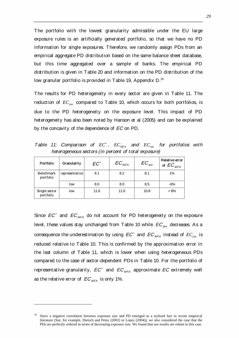
The results for PD heterogeneity in every sector are given in Table 11. The
reduction of simEC compared to Table 10, which occurs for both portfolios, is
due to the PD heterogeneity on the exposure level. This impact of PD
heterogeneity has also been noted by Hanson et al (2005) and can be explained
by the concavity of the dependence of EC on PD.
Table 11: Comparison of EC , MFAEC and simEC for portfolios withheterogeneous sectors (in percent of total exposure)
Portfolio Granularity EC MFAEC simECRelative error
of MFAEC
Benchmarkportfolio
representative 8.1 8.2 8.1 1%
low 8.0 8.0 8.5 -6%
Single sectorportfolio
low 11.6 11.6 10.8 +8%
Since EC and MFAEC do not account for PD heterogeneity on the exposure
level, these values stay unchanged from Table 10 while simEC decreases. As a
consequence the underestimation by using EC and MFAEC instead of simEC is
reduced relative to Table 10. This is confirmed by the approximation error in
the last column of Table 11, which is lower when using heterogeneous PDs
compared to the case of sector-dependent PDs in Table 10. For the portfolio of
representative granularity, EC and MFAEC approximate EC extremely well
as the relative error of MFAEC is only 1%.
29 Since a negative correlation between exposure size and PD emerged as a stylized fact in recent empiricalliterature (See, for example, Dietsch and Petey (2002) or Lopez (2004)), we also considered the case that thePDs are perfectly ordered in terms of decreasing exposure size. We found that our results are robust in this case.
30
In the single-sector portfolio, the approximation errors of the EC proxies are
positive, implying that the effect of PD heterogeneity is stronger than the
granularity effect, measured relative to the highly granular portfolio with
homogeneous sector PDs. As a consequence, the ASRF* model actually
overestimates EC.
In summary, the approximation errors for all portfolios considered vary
between -6% and +8%. For the benchmark portfolio they are always lower
than the corresponding values in Table 10 and for the single-sector portfolio
the estimates are more conservative. The results of Table 10 and Table 11
taken together demonstrate that the effect of PD heterogeneity
counterbalances the effect of granularity. In general it is not possible to
determine which of the two opposing effects dominates. For the portfolio with
a representative granularity in Table 11, both effects nearly cancel each other
out, which is a rather encouraging result. Granularity in this portfolio is still
conservatively measured since the underlying sample includes only the larger
exposures of a bank. Therefore, the effect of granularity for this portfolio is
arguably weaker than for portfolios of average granularity in real banks.
This suggests that for such portfolios, PD heterogeneity would tend to
overcompensate the granularity effect and EC and MFAEC would provide
conservative estimates. Further empirical work is warranted to confirm this
indicative result.
Our analysis has shown that PD heterogeneity on the exposure level improves
the performance of the analytic EC approximations relative to the situation of
a granular portfolio with (only) sector-dependent PDs. The reason is that PD
heterogeneity reduces the underestimation of EC that is caused by the
granularity of the portfolio. This effect is even stronger if larger exposures or
firms have lower PDs than smaller ones. Furthermore, PD heterogeneity
appears not to affect the relative difference between MFAEC and *EC .
8. Summary and Conclusions
The minimum capital requirements for credit risk in the IRB approach of
Basel II implicitly assume that banks portfolios are well diversified across
business sectors. Potential concentration risk in certain business sectors is

31
covered by Pillar 2 of the Basel II Framework which comprises the supervisory
review process.30 To what extent the regulatory minimum capital requirements
can understate economic capital is an empirical question. In this paper we
provide a tentative answer by using data from the German central credit
register. Credit risk is measured by economic capital in a multi-factor asset
value model by Monte Carlo simulations.
In order to measure the impact of concentration risk on economic capital, we
start in the empirical part with a benchmark portfolio that reflects average
sector exposures of the German banking system. Since the exposure
distributions across business sectors are similar in Belgium, France and Spain,
we expect that our main results also hold for other European countries.
Starting with the benchmark portfolio, we have successively increased sector
concentration, considering degrees of sector concentration which are observable
in real banks. The most concentrated portfolio contained exposures only to a
single sector. Compared with the benchmark portfolio, economic capital for the
concentrated portfolios can increase by almost 37% and be even higher in the
case of a one-sector portfolio. This result clearly underlines the necessity to
take inter-sector dependency into account for the measurement of credit risk.
We subjected our results to various robustness checks. We found that the
increase in economic capital may even be greater, contingent to the
dependence structure.
Since concentration in business sectors can substantially increase economic
capital, a tractable and robust calculation method for economic capital which
avoids the use of computationally burdensome Monte Carlo simulations is
desirable. For this purpose the theoretical part evaluates the accuracy of a
model developed by Pykhtin (2004) which provides an analytical
approximation of economic capital in a multi-factor framework. We have
applied a simplified, more tractable version of the model which requires only
sector-aggregates of exposure size, PD and expected loss severity. The
dependence structure is captured by the correlation matrix of the original
multi-factor model. Furthermore, we have evaluated the extent to which
EC , as the first of two components in the analytic approximation of
30 See BCBS (2004b), paragraphs 770-777.

32
economic capital, already provides a reasonable proxy of EC. EC refers to
the economic capital for a single-factor model in which the sector-dependent
asset correlations are defined by mapping the richer correlation structure of
the multi-factor model. The benchmark for the approximation quality is
always the EC of the original multi-factor model which is obtained from MC
simulations.
We have shown that the analytic approximation formulae perform very well
for portfolios with relatively granular and homogeneous sectors. This result
holds for portfolios with different sector concentrations and for various factor
weights and correlation assumptions. Furthermore, we have found that EC is
relatively close to the simulation-based economic capital for most of the
realistic input parameter tupels considered.
Finally, we explore the robustness of our results against the violation of two
critical model assumptions, namely infinite granularity in every sector and
sector-dependent PDs. We find that lower granularity and PD heterogeneity
on the single exposure level have two counterbalancing effects on the
performance of the analytic approximations for economic capital. The
reduction of granularity induces the analytic approximation formulae to have a
slight downward bias. In extreme cases of portfolios with the lowest
granularity permissible by EU large exposure rules, the downward bias
increases to 14%, depending on the sector structure of the portfolio.
Introducing heterogeneous PDs on the individual exposure level reduces
economic capital, but does not affect the analytic approximations. As a
consequence, the downward bias decreases. The relative error of the analytic
approximation, measured relative to the simulation-based EC figure, lies in a
range between 6% and +8%. In summary, we find that heterogeneity in
individual PDs and low granularity partly balance each other in their impact
on the performance of the analytic approximations. Which effect prevails
depends on the specific input parameters. Indicative results suggest that in
representative credit portfolios, PD heterogeneity will at least compensate for
the granularity effect which suggests that the analytic formulae approximate
EC reasonably well or err on the conservative side.

33
In the cases studied, it is possible to use the simplified version of the model
which provides analytic approximations of EC without sacrificing much
accuracy. This is an important result as it suggests that supervisors and banks
can reasonably well approximate their economic capital for their credit
portfolio by a relatively simple formula and without running computationally
burdensome Monte Carlo simulations.
Further research seems to be warranted, particularly in further advancing
Pykhtin s methodology in a direction which improves its approximation
accuracy without extending data requirements. This could be achieved, for
example, by exploring alternative ways to map the correlation matrix of the
multi-factor model into sector-dependent asset correlations.

34
References
BCBS (2004a), Basel Committee on Banking Supervision, Bank Failures inMature Economies , http://www.bis.org/publ/bcbs_wp13.pdf
BCBS (2004b), Basel Committee on Banking Supervision, InternationalConvergence of Capital Measurement and Capital Standards: A revisedFramework , http://www.bis.org/publ/bcbs107b.pdf.
BLUHM, C., L. OVERBECK, AND C. WAGNER (2003), An Introduction to CreditRisk Modeling, Chapman&Hall/CRC, p 297.
BURTON, S., S. CHOMSISENGPHET AND E. HEITFIELD (2005), The Effects ofName and Sector Concentrations on the Distribution of Losses forPortfolios of Large Wholesale Credit Exposures , paper presented atBCBS/Deutsche Bundesbank/ Journal of Credit Risk Conference inElville 18-19 November 2005.
CESPEDES, J.C.G., J.A DE JUAN HERRERO, A. KREININ, AND D. ROSEN (2005),A Simple Multi-Factor Adjustment , for the Treatment of
Diversification in Credit Capital Rules, submitted to the Journal ofCredit Risk.
COURIEROUX, C., J.-P. LAURENT, AND O. SCAILLET (2000), SensitivityAnalysis of Values at Risk , Journal of Empirical Finance, 7, pp 225-245.
DE SERVIGNY A. AND O. RENAULT (2002), Default correlation: Empiricalevidence , Standard and Poors Working Paper.
DIETSCH, M. AND J. PETEY (2002), The Credit Risk in SME Loan Portfolios:Modeling Issues, Pricing and Capital Requirements , Journal of Bankingand Finance, 26, pp 303-322.
DÜLLMANN, K. (2006), Measuring Business Sector Concentration by anInfection Model , Deutsche Bundesbank Discussion Paper (Series 2), No3.
FITCHRATINGS (2004), Default Correlation and its Effect on Portfolios ofCredit Risk", Credit Products Special Report.
GORDY, M. (2000), A Comparative Anatomy of Credit Risk Models , Journalof Banking and Finance, 24 (1-2), pp 119-149.
GORDY, M. (2003), A Risk-Factor Model Foundation for Ratings-Based BankCapital Rules , Journal of Financial Intermediation, 12, 199-232.
GUPTON, G., C. FINGER AND M. BHATIA (1997), CreditMetrics - TechnicalDocument .
HAHNENSTEIN, L. (2004), Calibrating the CreditMetrics Correlation Concept -Empirical Evidence from Germany , Financial Markets and PortfolioManagement, 18(4), 358-381.
HANSON, S., M.H. PESARAN, AND T. SCHUERMANN (2005), Firm Heterogeneityand Credit Risk Diversification , Working Paper(http://www.cesifo.de/DocCIDL/cesifo1_wp1531.pdf)
HESTON, L. and G. ROUWENHORST (1995), Industry and Country Effects inInternational Stock Returns , Journal of Portfolio Management, 53-59.
HIRSCHMANN, A. O. (1964), The Paternity of an Index , InternationalEconomic Review, 761-762.

35
JOINT Forum (1999), Risk Concentration Principles , Basel.
KRÜGER, U., M. STÖTZEL AND S. TRÜCK (2005), Time Series Properties of aRating System Based on Financial Ratios , Deutsche BundesbankDiscussion paper (series 2).
LOPEZ, J., (2004), The Empirical Relationship between Average AssetCorrelation, Firm Probability of Default and Asset Size , Journal ofFinancial Intermediation, 13, 265-283.
MARTIN, R. and T. WILDE (2002), Unsystematic Credit Risk , Risk,November, pp 123-128.
MERTON, R. (1974), On the Pricing of Corporate Debt: The Risk Structureof Interest Rates , Journal of Finance, 34, 449-470.
MOODY'S (2004), Moody's Revisits its Assumptions regarding CorporateDefault (and Asset) Correlations for CDOs , November.
PESARAN, M.H., T. SCHUERMANN AND B. TREUTLER (2005), The Role ofIndustry, Geography and Firm Heterogeneity in Credit RiskDiversification , NBER Working Paper.
PYKHTIN, M. (2004), Multi-Factor Adjustment , Risk, March, pp 85-90.
S&P (2004), Ratings Performance 2003 , S&P Special Report, p 40.
ZENG, B. and J. ZHANG (2001), Modeling Credit Correlation: EquityCorrelation is not Enough , Moody' s KMV Working Paper.

36
Appendix A
Table 12: GICS Classification Scheme: Broad Sector and Industry Groups
A: Energy A1: EnergyB: Materials B1: MaterialsC: Industrial C1: Capital goods
C2: Commercial Services and SuppliesC3: Transportation
D: Consumer Discretionary D1: Automobiles and ComponentsD2: Consumer Durables and ApparelD3: Hotels, Restaurants and LeisureD4: MediaD5: Retailing
E: Consumer Staples E1: Food and Drug RetailingE2: Food, Beverage and TobaccoE3: Household and Personal Products
F: Health Care F1: Health Care Equipment and ServicesF2: Pharmaceuticals and Biotechnology
G: Financials G1: BanksG2: Diversified FinancialsG3: InsuranceG4: Real estate
H: Information Technology H1: Software and ServicesH2: Technology Hardware & EquipmentH3: Semiconductors & SemiconductorEquipment
I: Telecommunication Services I1: Telecommunication ServicesJ: Utilities J1: Utilities
Table 13: Mapping NACE codes to GICS codes
2 (or more) -digitcode
Description Mapped to GICS
1 Agriculture and hunting E
2 Forestry B
5 Fishing E
10 Coal mining B
11 Crude petroleum and natural gas extraction A
12 Mining of uranium and thorium B
13 Mining of metal ores B
14 Other mining and quarrying B
15 Food and beverages manufacturing E
16 Tobacco manufacturing E
17 Textile manufacturing D
18 Textile products manufacturing D
19 Leather and leather products manufacturing D
20 Wood products D
21 Pulp, paper and paper products B
22 Publishing and printing C2

37
23 Manufacture of coke, refined petroleum products and nuclearfuel
A
24 (excl 244) Chemicals and chemical products manufacturing B
244 Pharmaceuticals F
25 Rubber and plastic manufacturing D
26 Other non-metallic mineral products B
27 Basic metals manufacturing B
28 Fabricated metal manufacturing B
29 Machinery and equipment manufacturing C1
30 Office machinery and computers manufacturing H
31 Electrical machinery manufacturing H
32 TV and communication equipment manufacturing H
33 Medical and optical instruments manufacturing F
34 Car manufacturing D
35 Other transport equipment manufacturing D
36 Furniture manufacturing D
37 Recycling J
40 Gas and electricity supply J
41 Water supply J
45 Construction C1
50 Car sales, maintenance and repairs D
51 Wholesale trade C2
52 (excl 5211,522,523)
Retail trade D
522, 523 Consumer staples E
55 Hotels and restaurants D
60 Land transport C3
61 Water transport C3
62 Air transport C3
63 Transport supporting activities and travel agencies C3
64 Post and telecommunication I
65 Financial institutions G1
66 Insurance G3
67 Support to financial institutions G1
70 Real estate G4
71 Machinery and equipment leasing manufacturing C1
72 Computer and related activities H
85 Health care and social work F
90 Sewage and refuse disposal J
96 Residential property management G4

38
Table 14: Comparison of sector concentrations, aggregated exposure valuesover banks in Germany, France, Belgium and Spain
Sector Germany France Belgium Spain
A1: Energy 0.18% 0.88% 0.05% 1,05%B1: Materials 6.01% 3.97% 7.45% 9,34%C: Industrial31 52.36% 63.82% 54.77% 48,53%C1: Capital Goods 11.53% 9.89% 32,90%C2: Commercial Services andSupplies 33.69% 37.74% 10,20%C3: Transportation 7.14% 7.14% 5,43%D: Consumer Discretionary 14.97% 11.91% 15.77% 18,60%E: Consumer Staples 6.48% 7.21% 7.05% 10,20%F: Health Care 9.09% 5.00% 5.64% 1,85%H1: Software and Services 3.20% 1.47% 1.86% 1,99%I1: Telecommunication Services 1.04% 1.91% 0.54% 2,67%J1: Utilities 6.67% 3.82% 6.87% 5,77%
Table 15: Correlation matrix based on MSCI EMU industry indices (based onweekly log return data covering the Nov 2002 - Nov 2003 period; inpercentages).
A B C1 C2 C3 D E F H I JA: Energy 100 62 66 43 62 67 78 70 50 47 72B: Materials 100 91 78 77 85 73 69 74 68 69C1: Capital Goods 100 76 80 92 74 68 81 72 75C2: Comm. svs &supplies 100 66 81 58 53 71 58 52C3: Transportation 100 78 68 59 70 65 64D: Consumerdiscretionary 100 71 66 86 72 70E: Consumerstaples 100 75 62 60 70F: Health Care 100 55 44 70H: Informationtechnology 100 69 58I: Telecommu-nication services 100 67J: Utilities 100
31 Aggregate of C1, C2 and C3 only used for comparison with French data. Not used in the analysis.

39
Appendix B
The multi-factor adjustment qt can be calculated according to Pykhtin
(2004) as follows:
(A1)1(1 )
1 ( )( ) ( )
2 ( ) ( )q
y N q
l yt v y v y y
l y l y
where y denotes the single systematic risk factor.
The first and second derivatives of the loss distribution function in a one-
factor model are
(A2) 1
1
( ) ( )
( ) ( )
N
s s ss
N
s s ss
l y w p y
l y w p y
where )(ˆ ' yps
and )(ˆ '' yps
are, respectively, the first and the second derivatives
of the conditional probability of default.
(A3)
1
2 2
1 1
2 2 2
( )( )
1 1
( )( )
1 1 1
s s ss
s s
s ss s ss
s s s
c N p c yp y N
c c
N p c yc N p c yp y N
c c c
.
The factor loading in the ASRF* model is denoted by cs which can be written
as s s sc r where s denotes the correlation between the composite sector
factor sY and the systematic factor Y in the ASRF* model.
The conditional variance ( ) var( | )v y L Y y

40
1 12
1 1
2 2 1 12
1
1
21 1
( ) ( ) , ( ) , ( ) ( )
( ) ( ) , ( ) ,
( ) ( )( ) ( ) ( )
1
S SY
s t s t s t st s ts t
SY
s s s s s sss
YS St st s
s t s t s tYs tst
v y w w N N p y N p y p y p y
w p y N N p y N p y
N p y p yv y w w p y N p y
22 2 1
21
1( ) 1 2 ( )
1
Ss
s s s ss s
rw p y N N p y
r
where 2N denotes the cumulative distribution function of the bivariate-
normal distribution andstY has the meaning of a conditional asset correlation
for two exposures in sectors t and s, conditional on Y . This conditional asset
correlation can be written as
2 2
-
1 - 1 -
s t st s tY
st
s t
r r r c cr
c c.

41
Appendix C
In Pykhtin (2004) the coefficients 1,..., Sb b are obtained by maximizing the
correlation between Y and the risk factors Y1,.....,YS which leads to the
following optimization problem:
1 ,..., ,1 1
maxS
S S
b b s s j js j
b .
subject to 2
1
1S
ss
b . The solution of this optimization problem is given by
,1
Ss
j s js
b .
is the Lagrange multiplier chosen to satisfy the constraint. Again there is no
unique solution for s. We follow Pykhtin who reported good results when
defining
1 1
21s s
s s s
s
N p r N qw N
r.
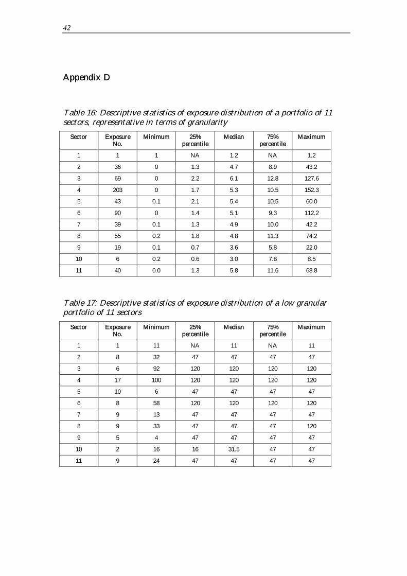
42
Appendix D
Table 16: Descriptive statistics of exposure distribution of a portfolio of 11sectors, representative in terms of granularity
Sector ExposureNo.
Minimum 25%percentile
Median 75%percentile
Maximum
1 1 1 NA 1.2 NA 1.2
2 36 0 1.3 4.7 8.9 43.2
3 69 0 2.2 6.1 12.8 127.6
4 203 0 1.7 5.3 10.5 152.3
5 43 0.1 2.1 5.4 10.5 60.0
6 90 0 1.4 5.1 9.3 112.2
7 39 0.1 1.3 4.9 10.0 42.2
8 55 0.2 1.8 4.8 11.3 74.2
9 19 0.1 0.7 3.6 5.8 22.0
10 6 0.2 0.6 3.0 7.8 8.5
11 40 0.0 1.3 5.8 11.6 68.8
Table 17: Descriptive statistics of exposure distribution of a low granularportfolio of 11 sectors
Sector ExposureNo.
Minimum 25%percentile
Median 75%percentile
Maximum
1 1 11 NA 11 NA 11
2 8 32 47 47 47 47
3 6 92 120 120 120 120
4 17 100 120 120 120 120
5 10 6 47 47 47 47
6 8 58 120 120 120 120
7 9 13 47 47 47 47
8 9 33 47 47 47 120
9 5 4 47 47 47 47
10 2 16 16 31.5 47 47
11 9 24 47 47 47 47

43
Table 18: Scaled PD distribution of a portfolio of 11 sectors, representative interms of granularity
Sector ExposureNo.
Minimum 25%percentile
Median 75%percentile
Maximum
1 1 1.0% NA 1.0% NA 1.0%
2 36 0.0% 0.5% 1.0% 2.0% 8.8%
3 69 0.1% 0.7% 1.4% 2.3% 8.9%
4 203 0.0% 0.9% 1.6% 3.0% 14.4%
5 43 0.1% 0.6% 1.4% 2.6% 5.7%
6 90 0.0% 0.7% 1.2% 2.5% 12.7%
7 39 0.0% 0.8% 1.9% 3.4% 5.1%
8 55 0.0% 0.3% 0.6% 1.3% 8.4%
9 19 0.0% 0.5% 1.6% 2.5% 5.5%
10 6 0.3% 2.4% 4.4% 5.7% 7.8%
11 40 0.0% 0.2% 3.4% 0.6% 2.4%
Table 19: Scaled PD distribution of a low granular portfolio of 11 sector
Sector ExposureNo.
Minimum 25%percentile
Median 75%percentile
Maximum
1 1 1.0% NA 1.0% NA 1.0%
2 8 0.3% 1.3% 1.3% 1.3% 4.2%
3 6 0.4% 1.5% 1.5% 1.5% 5.1%
4 17 0.1% 1.8% 1.8% 1.8% 5.9%
5 10 0.1% 1.5% 1.5% 1.5% 4.9%
6 8 0.4% 1.4% 1.4% 1.4% 4.7%
7 9 0.1% 1.7% 1.7% 1.7% 5.8%
8 9 0.1% 0.7% 0.7% 0.7% 2.4%
9 5 0.3% 1.2% 1.2% 1.2% 3.9%
10 2 2.4% 2.4% 2.4% 2.4% 2.4%
11 9 0% 0.3% 0.3% 0.3% 1%
Table 20: Quality distribution of German firms in the Bundesbank database
Rating grade AAA AA A BBB BB B
Share in percent 2 6 11 55 24 2
(unscaled) PDin percent
0.01 0.02 0.07 0.26 0.87 3.27


