
DEPARTMENT OF CIVIL ENGINEERING
UET LAHORE
LECTURE # 1 INTRODUCTION
SE-501 STRUCTURAL ANALYSIS

Teachers/Instructors:
1.Prof. Dr. Asif Hameed
2.Dr. Ali Ahmed
Class Rules:
1. Attendance: You are expected in each class, Attendance less than 75% will attribute to the WF grade.
2. Participation: Class participation and discussion will be encouraged and have 5% marks.
3. Cell phone: Preferably don’t bring in the class.
However, the use of mobile phone during lecture are strictly not allowed.
4. You are expected to produce your own work
5. Assignments should be submitted in proper folder.
SE-501 STRUCTURAL ANALYSIS Class Rules

INTRODUCTION
COURSE OUTLINE
Standard Stiffness Method:
Steps involved in the standard stiffness method for linear analysis of the
following elements:
Plane truss, space truss, Beam, plane frame, grillage and space
frame elements.
Computer software development for Pin-connected and Rigidly-
connected 3-D elements
Treatment of non-conforming joints, Condensation and sub-structuring
techniques. Three-dimensional modeling of multistory building
systems. Concept of symmetry. Super Members
Introduction to numerical methods and solution techniques
appropriate to discrete structural systems.

INTRODUCTION
COURSE OUTLINE
Finite Element Method
Introduction to the method, Stationary Principles, the Rayleigh Ritz
Method, and Interpolation. Displacement-Based Elements for Structural
Mechanics. The Isoperimetric Formulation.
Weighted Residual Methods and the Finite Element Method. Numerical
Error and Convergence in Finite Element Analysis
Assembly procedure for multiple ended members, Discretization of
Elements, Development of Element Stiffness matrices for the following
elements: Triangular and rectangular plane stress elements Triangular
and rectangular plate bending elements.
Assembly of plane stress and plate bending elements as a thin shell
element.
3. Introduction to approximate methods of analysis for skeletal,
continuum and composite space structures e.g. slab & shell analogies,
Equivalent Energy Method and Girder Analogy etc.

INTRODUCTION
REFERENCE BOOKS
1. A First Course in the Finite Element Method Daryl L. Logan
2. Concepts and Applications of Finite Element Analysis Cook, Malkus, and
Plesha
3. Fundamentals of Finite Element Analysis David V. Hutton
4. Finite Element Procedures By Bathe, 2nd Edition
5. Structural Analysis By Coates, Coutie and Kong.
6. The Finite Element Method: Volume-1 The Basis By Zienkiewicz and
Taylor, 5th Edition
7. The Finite Element Method using MATLAB By Kwon and Bang

INTRODUCTION
COMMON ANALYSIS METHODS

INTRODUCTION
THE PROCESS OF FINITE ELEMENT ANALYSIS

INTRODUCTION
The finite element method is a computational scheme to solve field problems in
engineering and science.
The fundamental concept involves dividing the body under study into a finite
number of pieces (subdomains) called elements (see Figure). Particular
assumptions are then made on the variation of the unknown dependent
variable(s) across each element using so-called interpolation or approximation
functions. This approximated variation is quantified in terms of solution values
at special element locations called nodes. Through this discretization process, the
method sets up an algebraic system of equations for unknown nodal values which
approximate the continuous solution. Because element size, shape and
approximating scheme can be varied to suit the problem, the method can
accurately simulate solutions to problems of complex geometry and loading and
thus this technique has become a very useful and practical tool.
FINITE ELEMENT ANALYSIS

INTRODUCTION
Many problems in engineering and applied science are governed by
differential or integral equations.
The solutions to these equations would provide an exact, closed-form
solution to the particular problem being studied.
However, complexities in the geometry, properties and in the boundary
conditions that are seen in most real-world problems usually means that an
exact solution cannot be obtained or obtained in a reasonable amount of
time.
Current product design cycle times imply that engineers must obtain design
solutions in a ‘short’ amount of time.
They are content to obtain approximate solutions that can be readily
obtained in a reasonable time frame, and with reasonable effort. The FEM
is one such approximate solution technique.
FINITE ELEMENT METHOD
INTRODUCTION
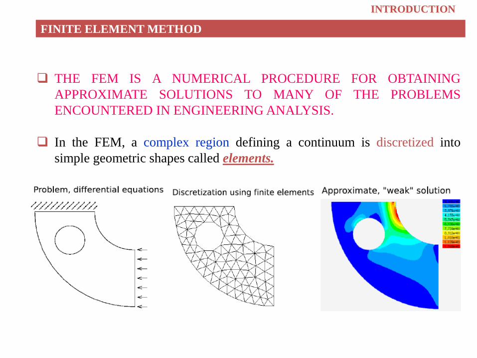
THE FEM IS A NUMERICAL PROCEDURE FOR OBTAINING
APPROXIMATE SOLUTIONS TO MANY OF THE PROBLEMS
ENCOUNTERED IN ENGINEERING ANALYSIS.
In the FEM, a complex region defining a continuum is discretized into
simple geometric shapes called elements.
FINITE ELEMENT METHOD

INTRODUCTION
The properties and the governing relationships are assumed over these
elements and expressed mathematically in terms of unknown values at
specific points in the elements called nodes.
An assembly process is used to link the individual elements to the given
system. When the effects of loads and boundary conditions are considered, a
set of linear or nonlinear algebraic equations is usually obtained.
Solution of these equations gives the approximate behavior of the
continuum or system.
The continuum has an infinite number of degrees-of-freedom (DOF), while
the discretized model has a finite number of DOF. This is the origin of the
name, finite element method.
FINITE ELEMENT METHOD

INTRODUCTION
The number of equations is usually rather large for most real-world
applications of the FEM, and requires the computational power of the
digital computer. THE FEM HAS LITTLE PRACTICAL VALUE IF
THE DIGITAL COMPUTER WERE NOT AVAILABLE.
Advances in and ready availability of computers and software has brought
the FEM within reach of engineers working in small industries, and even
students.
FINITE ELEMENT METHOD

INTRODUCTION
It is difficult to document the exact origin of the FEM, because the basic
concepts have evolved over a period of 150 or more years.
The term finite element was first coined by Clough in 1960. In the early
1960s, engineers used the method for approximate solution of problems in
stress analysis, fluid flow, heat transfer, and other areas.
The first book on the FEM by Zienkiewicz and Chung was published in
1967.
In the late 1960s and early 1970s, the FEM was applied to a wide variety of
engineering problems.
ORIGINS OF THE FINITE ELEMENT METHOD

INTRODUCTION
The 1970s marked advances in mathematical treatments, including the
development of new elements, and convergence studies.
Most commercial FEM software packages originated in the 1970s
(ABAQUS, ADINA, ANSYS, MARK) and 1980s (FENRIS, LARSTRAN
‘80)
The FEM is one of the most important developments in computational
methods to occur in the 20th century.
In just a few decades, the method has evolved from one with applications in
structural engineering to a widely utilized and richly varied computational
approach for many scientific and technological areas.
ORIGINS OF THE FINITE ELEMENT METHOD

INTRODUCTION
The range of applications of finite elements is too large to list, but to provide
an idea of its versatility we list the following:
Stress and thermal analyses of industrial parts such as electronic chips,
electric devices, valves, pipes, pressure vessels, automotive engines and
aircraft;
Analysis of dams, power plants and high-rise buildings;
Crash analysis of cars, trains and aircraft;
Fluid flow analysis of coolant ponds, contaminants, and air in ventilation
systems;
Electromagnetic analysis of antennas and transistors.
Analysis of surgical procedures such as plastic surgery, jaw reconstruction,
and many others.
This is a very short list that is just intended to give you an idea of the
breadth of application areas for the method. New areas of application are
constantly emerging.
APPLICATIONS OF FINITE ELEMENTS

INTRODUCTION
APPLICATIONS OF FINITE ELEMENT METHOD

INTRODUCTION
APPLICATIONS OF FINITE ELEMENT METHOD

INTRODUCTION
WHAT DOES A FINITE ELEMENT LOOK LIKE?

INTRODUCTION
GENERAL STEPS OF THE FEM
Step-1 Obtain a basic understanding of the problem you are attempting to
solve. Are any classical solutions (closed-form) available? Experimental
solutions are possible? Which modes of deformation do you expect to
significantly contribute to the structure’s behavior?
Step-2 Create model, select element types and discretize the problem
domain. This entails dividing the continuous structure into a finite number of
elements or regions over which the unknowns (displacements, in this class)
will be interpolated.
Some Basic Element Shapes

INTRODUCTION
GENERAL STEPS OF THE FEM
Step-3 Select an approximate displacement function within each element.
Linear, quadratic, or cubic polynomials are frequently used to interpolate
displacement values, within each element, from the element nodes. The
number of nodes increases with order.

INTRODUCTION
GENERAL STEPS OF THE FEM
Step-4 Describe the behavior of the physical quantities on each element.
Step-5 Connect (assemble) the elements at the nodes to form an
approximate system of equations for the whole structure.
Step-6 Solve the system of equations involving unknown quantities at the
nodes (e.g., displacements).
Step-7 Calculate desired quantities (e.g., strains and stresses) at selected
elements
FEM model for a gear tooth

INTRODUCTION
ADVANTAGES OF THE FINITE ELEMENT METHOD
Can readily handle complex geometry: The heart and power of the FEM.
Can handle complex analysis types:
Vibration
Transients
Nonlinear
Heat transfer
Fluids
Can handle complex loading:
Node-based loading (point loads).
Element-based loading (pressure, thermal, inertial forces).
Time or frequency dependent loading.
Can handle complex restraints:
Indeterminate structures can be analyzed.
Can handle bodies comprised of non-homogeneous materials:
Every element in the model could be assigned a different set of material
properties.

INTRODUCTION
ADVANTAGES OF THE FINITE ELEMENT METHOD
Can handle bodies comprised of non-isotropic materials:
Orthotropic
Anisotropic
Special material effects are handled:
Temperature dependent properties.
Plasticity
Creep
Swelling
Special geometric effects can be modeled:
Large displacements.
Large rotations.
Contact (gap) condition
Versatility– the method can be applied to various problems with
arbitrary problem domain shape, loading conditions, and boundary conditions.
Accuracy Control – Solution can be as accurate as desired provided that the
element formulation is proper. By increasing the number of elements (and thus
nodes) in the problem discretization (mesh), the solution should converge to the
exact or analytical solution.

INTRODUCTION
DISADVANTAGES OF THE FINITE ELEMENT METHOD
A specific numerical result is obtained for a specific problem. A general closed-form
solution, which would permit one to examine system response to changes in various
parameters, is not produced.
The FEM is applied to an approximation of the mathematical model of a system (the
source of so-called inherited errors.)
Experience and judgment are needed in order to construct a good finite element
model.
Input and output data may be large and tedious to prepare and interpret.
Numerical problems:
Round off and error accumulation.
Can help the situation by not attaching stiff (small) elements to flexible
(large) elements.
Susceptible to user-introduced modeling errors:
Poor choice of element types.
Distorted elements.
Geometry not adequately modeled.

INTRODUCTION
HOW CAN THE FEM HELP THE DESIGN ENGINEER?
The FEM offers many important advantages to the design engineer Easily applied to
complex, irregular-shaped objects composed of several different materials and having
complex boundary conditions.
Applicable to steady-state, time dependent and eigenvalue problems.
Applicable to linear and nonlinear problems.
One method can solve a wide variety of problems, including problems in solid
mechanics, fluid mechanics, chemical reactions, electromagnetics, biomechanics, heat
transfer and acoustics, to name a few.
General-purpose FEM software packages are available at reasonable cost, and can be
readily executed on microcomputers, including workstations and PCs.
The FEM can be coupled to CAD programs to facilitate solid modeling and mesh
generation.
Many FEM software packages feature GUI interfaces, auto-meshers, and sophisticated
postprocessors and graphics to speed the analysis and make pre and post-processing
more user-friendly.

INTRODUCTION
HOW CAN THE FEM HELP THE DESIGN ORGANIZATION?
Simulation using the FEM also offers important business advantages to the design
organization:
Reduced testing and redesign costs thereby shortening the product
development time.
Identify issues in designs before tooling is committed.
Refine components before dependencies to other components prohibit changes.
Optimize performance before prototyping.
Discover design problems before litigation.
Allow more time for designers to use engineering judgment, and less time
“turning the crank.”


