
Accepted Manuscript
Scale dependent solute dispersion with linear isotherm in heterogeneous medi-um
Mritunjay Kumar Singh, Pintu Das
PII: S0022-1694(14)00983-4DOI: http://dx.doi.org/10.1016/j.jhydrol.2014.11.061Reference: HYDROL 20076
To appear in: Journal of Hydrology
Received Date: 30 September 2014Revised Date: 20 November 2014Accepted Date: 22 November 2014
Please cite this article as: Singh, M.K., Das, P., Scale dependent solute dispersion with linear isotherm inheterogeneous medium, Journal of Hydrology (2014), doi: http://dx.doi.org/10.1016/j.jhydrol.2014.11.061
This is a PDF file of an unedited manuscript that has been accepted for publication. As a service to our customerswe are providing this early version of the manuscript. The manuscript will undergo copyediting, typesetting, andreview of the resulting proof before it is published in its final form. Please note that during the production processerrors may be discovered which could affect the content, and all legal disclaimers that apply to the journal pertain.

Scale dependent solute dispersion with linear isotherm
in heterogeneous medium
Mritunjay Kumar Singh1 and Pintu Das
2
Abstract
This study presents an analytical solution for one-dimensional scale dependent solute
dispersion with linear isotherm in semi-infinite heterogeneous medium. The
governing advection-dispersion equation includes the terms such as advection,
dispersion, zero order production and linear adsorption with respect to the liquid and
solid phases. Initially, the medium is assumed to be polluted as the linear combination
of source concentration and zero order production term with distance. Time dependent
exponentially decreasing input source is assumed at one end of the domain in which
initial source concentration is also included i.e., at the origin. The concentration
gradient at the other end of the aquifer is assumed zero as there is no mass flux exists
at that end. The analytical solution is derived by using the Laplace integral transform
technique. Special cases are presented with respect to the different forms of velocity
expression which are very much relevant in solute transport analysis. Result shows an
excellent agreement between the analytical solutions with the different geological
formations and velocity patterns. The impacts of non-dimensional parameters such as
Peclet and Courant numbers have also been discussed. The results of analytical
solution are compared with numerical solution obtained by explicit finite difference
method. The stability condition has also been discussed. The accuracy of the result
has been verified with root mean square error analysis. The CPU time has also been
calculated for execution of Matlab program.
Keyword: Analytical/Numerical solution, solute, dispersion, heterogeneous, aquifer,
aquitard

1, 2 Department of Applied Mathematics, Indian School of Mines, Dhanbad
Email: 1 [email protected] and 2 [email protected]
1. Introduction
Pollutants can originate from either point sources or nonpoint sources. Once
the pollutants enter into the subsurface region, they may have every possibility to
reach shallow aquifers in due course of time. Meanwhile, some pollutants adsorbed by
soil and some dissolved in water, and some are transported downstream which moves
along flow pathways. These pollutants are very often found in groundwater as a result
of waste disposal or leakage of urban sewage and industrial wastes, surficial
applications of pesticides and fertilizers used in agriculture, atmospheric deposition or
accidental releases of chemicals on the earth surface. Pollutants dissolved in
groundwater typically experience complex physical and chemical processes such as
advection, diffusion, chemical reactions, adsorption, and biodegradation & decay etc.
To predict the fate and transport of solutes in groundwater through understanding and
simulating these processes is very complex. The transformation of these
phenomenons in mathematical equation commonly represents Advection Dispersion
(AD) equation which depends upon fundamental equation of conservation of mass.
We may rely on AD equation for describing the migration and fate of pollutants in
groundwater bodies supported by existing literature.
There are considerable body of literature available on solute transport which
may be enlisted and it has been dealt with AD equation since last four five decades.
Ebach and white (1958) studied the longitudinal dispersion problem for an input
concentration that varies periodically with time. Ogata and Bank (1961) discussed for
the constant input concentration. Hoopes and Harleman (1965) studied the problem of
dispersion in radial flow from fully penetrating well; homogeneous, isotropic non

adsorbing confined aquifers. Bruce and Street (1967) established both longitudinal
and lateral dispersion effect with semi-infinite non adsorbing porous media in a steady
unidirectional flow fluid for a constant input concentration. Bear (1972) studied the
transport of solutes in saturated porous media is commonly described by the advection
-dispersion equation. Marino (1974) obtained the input concentration varying
exponentially with time. Hunt (1978) proposed the perturbation method to
longitudinal and lateral dispersion in non-uniform, steady and unsteady seepage flow
through heterogeneous aquifers. Wang et al. (1978) studied the concentration
distribution of a pollutant arising from instantaneous point source in a two
dimensional water channel with non-uniform velocity distribution. Kumar (1983)
discussed the dispersion of pollutants in semi-infinite porous media with unsteady
velocity distribution. Kumar (1983) studied the significant application of advection
diffusion equation. Lee (1999), Batu (1989), and Batu (1993) presented two
dimensional analytical solutions considering solute transport for a bounded aquifer by
adopting Fourier analysis and Laplace transform technique. Aral and Liao (1996)
obtained a general analytical solution of the two dimensional solute transport equation
with time dependent dispersion coefficient for an infinite domain aquifer. Serrano
(1995) established the scale-dependent models to predict mean contaminant
concentration from point sources i.e., well injection, and non-point sources i.e.,
ground surface spills in heterogeneous aquifers. Schafer et al. (1996) presented
transport of reactive species in heterogeneous porous media. Zoppou and Knight
(1997) explored the analytical solutions for advection and advection-diffusion
equations with spatially variable coefficients in which the diffusion coefficient
proportional to the square of the velocity concept employed. Delay et al.(1997)
predicted solute transport in heterogeneous media from results obtained in

homogeneous ones: an experimental approach. Liu et al. (1998) evaluated an
analytical solution to the one-dimensional solute advection-dispersion equation in
multi-layer porous media by using a generalized integral transform technique. Verma
et al. (2000) discussed an overlapping control volume method for the numerical
solution of transient solute transport problems in groundwater. Diaw et al. (2001)
presented one dimensional simulation of solute transfer in saturated-unsaturated
porous media using the discontinuous finite elements method. Saied and Khalifa
(2002) presented some analytical solutions for groundwater flow and transport
equation. McKenna et al. (2003) discussed the longitudinal and transverse
dispersivities in three dimensional heterogeneous fractured media. Ptak et al.(2004)
reviewed over the tracer investigation of heterogeneous porous media and stochastic
modelling of flow and transport of contaminant in the groundwater flow. Huang et al.
(2006) employed a parabolic distance-dependent dispersivity for solving one
dimensional fractional ADE. Kim and Kavvas (2006), Huang et al. (2008), and Du et
al. (2010) presented transport processes in heterogeneous geological media by
Fractional Advection-Diffusion Equation (FADE).
Liu et al. (2007) explored the numerical experiments to investigate potential
mechanisms behind possible scale-dependent behavior of the matrix diffusion for
solute transport in fractured rock. Chen et al. (2008) developed an analytical solution
to solute transport with the hyperbolic distance-dependent dispersivity in a finite
column. Guerrero et al. (2009) studied the formal exact solution of the linear
advection-diffusion transport equation with constant coefficients for both transient
and steady-state regimes by using the integral transform technique. Guerrero and
Skaggs (2010) obtained a general analytical solution for the linear, one-dimensional
advection-dispersion equation with distance-dependent coefficients in heterogeneous

porous media. Chen and Liu (2011) presented the generalized analytical solution for
one-dimensional solute transport in finite spatial domain subject to arbitrary time-
dependent inlet boundary condition. Hayek (2011) presented a non-linear convection-
diffusion reaction equation, considered as generalised Fisher equation with convective
terms. Exact and traveling-wave solutions for convection-diffusion-reaction equation
with power-law nonlinearity in which density independent and density dependent
diffusion were studied. Roubinet et al. (2012) developed the semi analytical solution
for the Fracture-matrix interactions of solute transport in fractured porous media and
rocks. Ranganathan et al. (2012) analysed the modeling and numerical simulation
study of density-driven natural convection during geological CO2 storage in
heterogeneous formations by using Sequential Gaussian Simulation method. Davit et
al. (2012) developed the transient behavior of homogenized models for solute
transport in two-region heterogeneous porous media. Chen et al. (2012) solved multi-
species advective–dispersive transport equations sequentially coupled with first-order
decay reactions. Singh et al. (2012) discussed the analytical solution for the one
dimensional heterogeneous porous media. Gao et al. (2012) developed the mobile-
immobile model (MIM) with an asymptotic dispersivity function of travel distance to
embrace the concept of scale-dependent dispersion during solute transport in finite
heterogeneous porous media.
Recently, You and Zhan (2013) studied the semi-analytical solution for solute
transport in a finite column is developed with linear-asymptotic or exponential
distance-dependent dispersivities and time-dependent sources. Guerrero et al. (2013)
presented analytical solutions of the advection–dispersion solute transport equation
solved by the Duhamel theorem with the time dependent boundary condition. van
Genuchten et al. (2013) presented a series of one- and multi-dimensional solutions of
the standard equilibrium advection-dispersion equation with and without terms
accounting for zero-order production and first-order decay. Vasquez et al. (2013)
introduced the modeling flow and reactive transport to explain mineral zoning in the
Atacama salt flat aquifer. Maraqa and Khashan (2014) established the effected of the
single-rate nonequilibrium heterogeneous sorption kinetics in the modeling of the
solute transport. Singh and Kumari (2014) presented one-dimensional contaminant
prediction along unsteady groundwater flow in aquifer with unit Heaviside type input
concentration. Fahs et al. (2014) explored extensively about a new benchmark semi-
analytical solution for verification of density-driven flow codes in porous media with
synthetic square porous cavity subjected to different salt concentration at its vertical
wall.
The traditional advection-dispersion equation is a standard model for solute
transport. Analyses of many solute transport problems required the use of
mathematical models corresponding with the application. Analytical models are useful
for providing physical insight to the system. Initial or approximate studies of
alternative pollution scenarios may be conducted to investigate the effects of various
parameters included in transport processes through the modelling approach.
The objective of the present work is to apply the Laplace integral transform technique
for solving one dimensional AD equation with zero order production term in which
linear isotherm concept is employed. The AD equation is solved under the initial and
boundary conditions taken into consideration. The heterogeneous medium is taken
into consideration in which the velocity is the function of the space as well as time
dependent. The dispersion is directly proportional to the square of the seepage
velocity employed. The various transformations are used for reducing the problem
into the simplest form. The exponentially decreasing and increasing form of the flow

pattern with respect to the time are considered. The non-dimensional Peclet and
courant numbers are also studied. The equilibrium relationship between the Peclet and
courant number are also depicted. The numerical solution is obtained by explicit finite
difference method in which the stability condition has also been discussed. The
accuracy of the result has been verified with root mean square error analysis.
2. Mathematical Formulation
The solute transport in heterogeneous porous media is generally modelled by
assuming a time as well as space dependent spatially average transport velocity and
solute dispersion, linear equilibrium adsorption, and first-order decay.
Mathematically, the partial differential equation for a semi-infinite heterogeneous
medium can be written as
1c n F cD uc
t n t x xγ
∂ − ∂ ∂ ∂ + = − +
∂ ∂ ∂ ∂ (1)
The simplest expression for the linear isotherm can be written as
dF k c= (2)
where, 2 1D L T
− is the longitudinal dispersion coefficient(i.e. representing
longitudinal dispersion), 3c ML
− is the volume averaged dispersing solute
concentration in the liquid phase, 3F ML
− is the volume averaged dispersing solute
concentration in the solid phase, 1u LT
− is the unsteady uniform downward pore
seepage velocity, [ ]x L is a longitudinal direction of flow , [ ]t T is time, 3 1ML Tγ − −
is the zero order production rate coefficients for solute production in the liquid phase,
n is the porosity of the different geological formation such as aquifer and aquitard etc.
and dk is arbitrary constant.
Equation (1) is solved analytically with the following initial and boundary conditions:
( ), 0 i
xc x c
u
γ= + 0, 0x t> = (3)
( ) ( )00, expic t c c tλ= + − ; 0, 0t x> = 4(a)
0c
x
∂=
∂; x → ∞ 4(b)
where, 1Tλ − is the decay constant.
Using equation (2), Equation (1) can be written as
c cR D uc
t x xγ
∂ ∂ ∂ = − +
∂ ∂ ∂ (5a)
where, 1
1 d
nR k
n
−= + (5b)
is the retardation factor.
However, for the longitudinal direction of the unsteady pollutant inflow into the
groundwater, the advection dispersion equations have spatially variable coefficients.
The variable coefficients for the conservative pollutants where the mass of the
injected pollutant is conserved and for the non-conservative pollutants where the
pollutant gets decayed or grows, resulting in increasing or decreasing the mass. If the
velocity field varies linearly with distance, and the dispersion coefficient is
proportional to the square of the velocity, and therefore proportional to the square of
the distance, then the concept (Zoppou and Knight, 1997) is employed as
( )( )0 1u u f mt x= + (6a)
and the dispersion parameter is proportional to a power of the seepage velocity which
ranges between 1 and 2 by Freeze and Cherry (1979). In the present analysis, due to
heterogeneity, power or indices is considered 2 and written as
( )( )22
01D D f mt x= + (6b)
Now, Using equations (6a) and (6b), equation (5a) can be written as
( )R c
f mt t
∂=
∂( )( ) ( )
2
0 0 01 1c
D f mt x u x cx x
γ∂ ∂
+ − + + ∂ ∂
(7a)
where, ( )0
f mt
γγ = (7b)
By introducing a new time variable as
( )0
t
T f mt dt= ∫ , (8)
Equation (7a) becomes
cR
T
∂=
∂( )( ) ( )
2
0 0 01 1c
D f mt x u x cx x
γ∂ ∂
+ − + + ∂ ∂
(9)
Again, by using the transformation as
( )2log 2 1Y x x= + + , (10)
Equation (9) becomes
cR
T
∂=
∂( ) ( )
2
0 0 1 0 024 2
c cD f mt u f mt u c
Y Yγ
∂ ∂− − +
∂ ∂ (11a)
where, ( ) ( )01
0
1D
f mt f mtu
= − (11b)
Now, by using another transformation as
( )( )
11
2
f mtZ dY
f mt= ∫ , (12)
Equation (11a) becomes
( )( )2
1
f mt cR
f mt T
∂=
∂
( )( )
( )( )
2
0 0 0 02
1 1
f mt f mtc cD u u c
Z Z f mt f mtγ
∂ ∂− − +
∂ ∂ (13)
By using the another time variable as
( )( )
2
1*
0
t f mtT dT
f mt= ∫ , (14)

Equation (13) becomes
*
cR
T
∂=
∂
( )( )
( )( )
2
0 0 0 02
1 1
f mt f mtc cD u u c
Z Z f mt f mtγ
∂ ∂− − +
∂ ∂ (15)
By using the transformations given in equations (8), (10), (12) and (14), initial and
boundary conditions (3), (4a) and (4b) can be written as follows:
( ),0c Z =( )( )
0
0 1
1 exp ;i
f mtc Z
u f mt
γ + − −
*0, 0Z T> = (16a)
i.e., ( ), 0c Z =
1
0 0
0 0
1 exp 1 ;i
Dc Z
u u
γ− + − − −
*0, 0Z T> = (16b)
i.e., ( ), 0c Z = 0 0
0 0
1 ;i
Dc Z
u u
γ + +
*0, 0Z T> = (17)
( ) ( )* *
00, 1ic T c c Tλ= + − ; * 0, 0T Z> = (18a)
0c
Z
∂=
∂; Z → ∞ (18b)
By introducing a new transformation as
( )*,c Z T = ( ) ( )( )
2* *0 0
02
0 0 1
1, exp
2 4
f mtu uK Z T Z u T
D R D f mt
− +
0
0u
γ+ (19)
Equation (15) becomes
2
0* 2
K KR D
T Z
∂ ∂=
∂ ∂ (20)
and the corresponding initial and boundary conditions given in (17),(18a) and (18b)
respectively can be written as follows:
( ), 0K Z =0
020 0 0
0 0 0
1 ;
uZ
D
i
Dc Z e
u u u
γ γ − + + −
*0, 0Z T> = (21)
( )*0,K T = ( )*00
0
1ic c Tu
γλ
− + −
( )
( )
2*0
020 1
1
4
f mtuu T
R D f mte
+ * 0, 0T Z> = (22a)

0
02
KuK
Z D
∂= −
∂; Z → ∞ (22b)
Laplace integral transform technique is now employed and the solution can be
obtained as follows:
( )*,c Z T = * * *0 00 0
0 0
( , ) ( , ) exp2
i
uc c F Z T c G Z T Z T
u D
γλ φ
+ − − −
* * *0 0 0 0
0 0 0
1 ( , ) ( , ) exp2
i
D uH Z T c I Z T Z T
R u u D
γ γφ
+ + − − −
2 2* *0 0 0 0
0 0 0 02 4 2 4 *0 0 0 0
0 0 0 0
1 exp2
u u u uZ T Z T
D RD D RD
i
D uc e Ze Z T
u u u D
γ γφ
− − − −
+ − + + −
2*0 0
0 02 4* *0 0 0
0 0
1 exp2
u uZ T
D RDD uT e Z T
R u D
γφ
− −
− + −
0
0u
γ+ (24)
where,
( )*,F Z T = * *
*0 0
1 1 1exp
2 2
R RT Z erfc Z T
D D T
φφ φ
− −
* *
*0 0
1 1 1exp
2 2
R RT Z erfc Z T
D D T
φφ φ
+ + +
(25a)
( )*,G Z T = *
0
12
4
RT Z
Dφ
φ
−
* *
*0 0
1 1exp
2
R RT Z erfc Z T
D D T
φφ φ
− −
*
0
12
4
RT Z
Dφ
φ
+ +
* *
*0 0
1 1exp
2
R RT Z erfc Z T
D D T
φφ φ
+ +
(25b)
( )
20* * * *0 0 0 0
*0 0 0 0 00 0
1 1, exp
2 4 2 2 2
RD u u u uR RH Z T T Z T Z erfc Z T
u D RD D DRD D RT
= − − −
20 * * *0 0 0 0
*0 0 0 0 00 0
1 1exp
2 4 2 2 2
RD u u u uR RT Z T Z erfc Z T
u D RD D DRD D RT
+ + + +
(25c)
( )*,I Z T =2
* *0 0 0
*0 0 0 0
1 1 1exp
2 4 2 2 2
u u uRT Z erfc Z T
RD D D D RT
− −
2
* *0 0 0
*0 0 0 0
1 1 1exp
2 4 2 2 2
u u uRT Z erfc Z T
RD D D D RT
+ + +
(25d)

( )( )
2
002
0 1
1
4
f mtuu
R D f mtφ
= +
(25e)
Due to the increasing human activities on the earth surface which causes the
pollution, get into the subsurface bodies, an appropriate boundary condition is
represented by the mixed type boundary condition. The mixed type boundary
condition is also termed as third type or Cauchy type boundary condition. Hence, the
analytical model can further be discussed with Cauchy type boundary condition
instead of Dirichlet type boundary condition and therefore, by considering Cauchy
type boundary condition at the origin i.e., at 0x = as
( )0 expi
cD uc u c c t
xλ
∂− + = + − ∂
at 0, 0t x> = (26)
Model is solved analytically with same procedure and the solution can be obtained as
follows:
( )*,c Z T = ( )* *0 0
0 0
, exp2
uK Z T Z T
D u
γφ
− +
(27)
where,
( )*,K Z T = * *0 00 0
0 0
2( , ) ( , )i
Dc c F Z T c G Z T
qu u
γλ
−+ − −
*0 0 0 0
0 0 0
21 ( , )i
D q Dc H Z T
qu R u u
γ γ − + − +
*0 0 0
0 0
21 ( , )
D DI Z T
qu R u
γ + +
0 0 * *00 1 0 12
00
4( , ) ( , )i
D RDc c F Z T c G Z T
uqu
γλ
− + − −
0 0 *0 0 012
0 00
41 ( , )i
D RD q Dc H Z T
R u uqu
γ γ − + − +
0 0 0 *012
00
41 ( , )
D RD DI Z T
uRqu
γ − +
2
* *0 0 0 0
0 0 0
1 exp2 4
D u uT Z T
R u D RD
γ − + − +
2
*0 0 0 0 0
0 0 0 0 0
1 exp2 4
i
D u uc Z Z T
u u u D RD
γ γ + − + + − +
(28a)

( )*
1 ,F Z T =2
**
1exp
4
Z
TTπ
−
* *
*0 0
1 1exp
2 2
R RT Z erfc Z T
D D T
φ φφ φ
+ − −
* *
*0 0
1 1exp
2 2
R RT Z erfc Z T
D D T
φ φφ φ
+ + +
(28b)
( )*
1,G Z T =
* 2
*exp
4
T Z
Tπ
−
( )* * * *
*0 0
1 1 11 2 exp
24
R RT T T Z erfc Z T
D D T
φφ φ φ φ
φ
+ − + − −
( )* * * *
*0 0
1 1 11 2 exp
24
R RT T T Z erfc Z T
D D T
φφ φ φ φ
φ
+ + + + +
(28c)
( )*
1 ,H Z T =2
**
1exp
4
Z
TTπ
−
2
* *0 0 0 0
*0 0 00 0
1 1exp
4 2 24 2
u u u uRT Z erfc Z T
RD D DD R D RT
+ − −
2* *0 0 0 0
*0 0 00 0
1 1exp
4 2 24 2
u u u uRT Z erfc Z T
RD D DD R D RT
+ + + (28d)
and,
( )* 2
*
1 *, exp
4
T ZI Z T
Tπ
= −
2
0 *0 0
0 0 0
12 2 2
RD u uZ T
u D D R
+ − +
2* *0 0 0
*0 0 0 0
1 1exp
4 2 2 2
u u uRT Z erfc Z T
RD D D D RT
− −
2 2
0 * *0 0 0 0
0 0 0 0 0
1 exp2 2 2 4 2
RD u u u uZ T T Z
u D D R RD D
− − + +
*0
*0 0
1 1
2 2
uRerfc Z T
D D RT
+
(28e)
3. Numerical Solution
Towler and Yang (1979) explored about the two possible global errors for the
numerical solution of the transport equation as 1) Root mean square average error
(RMSE) of all grid points for the particular time domain and 2) the maximum
absolute error across the time level. Roberts and Selim (1984) used the root mean

square method to calculate the average error at each nodal point of the grid. Ataie-
Ashtiani et al. (1999) studied the expansion of the Taylors series of the solute
concentration along the advection dispersion equation used for determining the
truncation error in one dimension. Zheng and Bennett (2002) presented dispersion
coefficients and components in global and local coordinate system change with
respect to their respective angles. Ataie-Ashtiani and Hosseini (2005) presented the
explicit finite difference methods for two dimension advection dispersion equation
associated with the numerical errors.
Hayek (2011) studied non-linear convection-diffusion-reaction equation with power
law nonlinearity in which the time-dependent velocity in the convection term is also
discussed. Fahs (2014) investigated the semi-analytical solution for the advection
dispersion equation using the Fourier-Galerkin method and validated the result of the
analytical solution with the numerical ones. Deng et al., (2014) compared the
analytical solution and eigenvalue system of the numerical solution for the solute
transport model with multi-layered porous media with generalized boundary
conditions. Bakker (1999) developed the analytical and numerical model for the
groundwater flow in multi aquifer system.
The advection dispersion equation defined in equation (15) expressed for the semi-
infinite medium. In order to solve by the finite difference technique medium change
into a finite medium by using suitable transformation
( )1 expz Z= − − (29)
Substituting equation (29) in equation (15) gives
( ) ( )2
2
0 1 1 1* 21 1
c c cR D z D z u c
T z zγ
∂ ∂ ∂= − − − − +
∂ ∂ ∂ (30a)
where, 1 0 0
D D u= + , ( )( )1 0
1
f mtu u
f mt= and
( )( )1 0
1
f mt
f mtγ γ= (30b)

Initial and boundary conditions as follows
( ) 0 0
0 0
1,0 1 log
1i
Dc z c
u u z
γ = + +
− ; *0, 0z T> = (31)
( ) ( )* *
00, 1ic T c c Tλ= + − ; *0, 0z T= > (32a)
0c
z
∂=
∂; *1, 0z T= > (32b)
The transport equation such as advection-dispersion equation and dispersion equation,
numerical dispersion is a well known consequence of truncation errors which is
introduced by the discretization of the model equation. Taylor’s expansion is used for
getting the finite difference equation (Mickley et al., 1957; Lantz 1971). The general
form of the explicit finite difference approximation with forward time and central
space forward difference scheme is used in the equation (30) together with initial and
boundary conditions given in equation (31), 32 (a) and 32 (b) which is approximated
as follows:
( ) ( )
( )( )
*2* 01
, 1 , 1, , 1, 2
**1 1
1, 1,
1 1 2
12
i j i j i j i j i j
i j i j
Du Tc T c z c c c
R R z
D Tz c c T
R z R
γ
+ + −
+ −
∆ = − ∆ + − − +
∆
∆− − − + ∆
∆
(33)
0 0,0
0 0
11 log
1i i
i
Dc c
u u z
γ = + −
− ; 0i > (34)
( )*
0, 0 1j i jc c c Tλ= + − ; 0j > (35a)
, 1,M j M jc c −= ; 0j > (35b)
The boundary conditions (26) can be written as
( )*
0, 1, 0
11
1 1
ij j i j
i i
zc c c c T
z zq
q q
λ∆
= + + − ∆ ∆+ +
(36a)
where,

( )2
*0 0
2
0 0
1D D
q mTu u
= + − (36b)
where the subscripts i and j refers to space and time respectively and [ ]*T T∆ is the
time increment, [ ]z L∆ is the space increment in equation (33).
The space domain z and time domain *T are discretized by a rectangular grid points
( )*,i jz T with mesh-size * and z T∆ ∆ respectively. Hence, one can write as follows:
1 0, 1, 2,..., , 0, 0.2i i
z z z i M z z−= + ∆ = = ∆ =
* * * * *
1 0, 1, 2,..., I, 0, 0.001j jT T T j T T−= + ∆ = = ∆ =
The contaminant concentration at a point for the space i
z with thj time step *T
defined by ,i jc .
3.1 Stability Analysis
Errors occur due to neglecting the higher order terms in finite difference
approximations. These errors show about the solution instability or numerical
inaccuracy. The solution of advection dispersion equation using explicit Finite
difference method, resulting as some truncation errors and the effect of these errors
has been demonstrated by comparing the analytical solution with the numerical one. If
the stability conditions are satisfied then our numerical solutions are convergent. The
finite difference method is said to be convergent if the discritization error approaches
zero as the grid spacing *T∆ and z∆ tend to zero. Here we used the forward
difference in time for the first order derivative of the with respect to time which
contains the first order accuracy. Stability test of finite difference scheme proposed by
a matrix method (Smith, 1978) and this technique was used by Notodamorjo et. al
(1991). The finite difference scheme of the governing partial differential equation of
parabolic type can be rearranged as

( ) ( ) ( ) *1, 1 1, , 1,
2i j i j i j i j
c c c c TR
γβ ξ α β β ξ+ − += + + − + − + ∆ (37a)
where, *11u
TR
α = − ∆ ,*
0
2
D T
R zβ
∆=
∆ and
*
1
2
D T
R zξ
∆=
∆ (37b)
In matrix form of equation (37a) can be written as
[ ] [ ]1j j
c A c+
= *1 TR
γ+ ∆ (38)
where, matrix A contains all the constant.
The difference equation is stable if the modulus of eigenvalues of A must have less
than or equal to unity i.e., 1µ ≤ , where µ is the eigenvalue of the matrix A .
On applying the Gerschgorin circle method, the stability criteria for the time step is
obtained as
*
01
2
1
2
2
TDu
R R z
∆ ≤
+ ∆
(39)
The numerical solution has been obtained for 0.2z∆ = and * 0.001T∆ = . It has been
observed that the stability criterion has been satisfied for the value of *T∆ .
4. Accuracy
Even if the finite difference equation is consistent and stable, the collective truncation
error may cause inaccuracies in the numerical solution. The accuracy of a finite
difference scheme is largely dependent on the magnitude of the truncation error. The
accuracy of the schemes examined in this work will also be described by comparing
the analytical (i.e., exact) and numerical solution at each nodal point. The root mean
square (RMS) method is used to calculate the average error at each point. The RMS
error is given by

2
1
1RMS
N
i
i
cN =
= ∆∑ (40)
where, analytical numerical
c c c∆ = −
The difference between the analytical and numerical results for the solute
concentration at the different point is denoted by c∆ and N is represented by the
number of data. Root mean square error was used to measure the performance of
numerical method against the exact solution of the advection dispersion equation in
the given problem.
5. Numerical Results, Discussion and Application
The various input values available in the hydrological literature reported by
Singh and Kumari (2014), the analytical solution given in equation (24) has been
computed for the following set of input data:
2
0 0 0 00.01, 1.0, 0.7 (km/year), 0.1(km /year), 0.0005(/km), 0.002ic c u D γ λ= = = = = =
2.5, 0.32(Gravel),0.37(Sand),0.55(Clay), 0.01(/year)d
k n m= = = . These input values
satisfy the boundary conditions which have been taken into consideration. The
pollutants concentration distribution patterns have been predicted for exponentially
decreasing and increasing forms of velocity pattern and their corresponding new time
variable. Mathematically, these are enlisted as follows:
(i) ( ) exp( )f mt mt= − (41)
and
( ) ( )2
* 20 0
2
00
21 1
2
mt mtD DT t e e
mumu
− −= + − − − (42)
(ii) ( ) exp( )f mt mt= , (43)
and

( ) ( )2
* 20 0
2
00
21 1
2
mt mtD DT t e e
mumu= + − + − . (44)
The pollutant concentration distribution pattern has been predicted for the time period
of 4th, 6th, and 8th year respectively. The same has also been predicted in a finite
domain 0 2.0x≤ ≤ (km) for the different geological formations such as sand, clay and
gravel. The pollutant distribution has also been discussed with reference to the non-
dimensional Peclet and Courant numbers. Figure 1, shows that the solute behaviour
for the aquifer (gravel) and aquitard (clay) formations increases with the time and
decreases with respect to the distance. The properties of geological formations are
different and therefore, aquifer generally contains more significant amount of water
and transmit more water as compare to aquitard. The pollutant concentration is higher
in the aquitard in compare to the aquifer at each of the positions. A pollutant
concentration goes on decreasing with the distance in both the geological formations
and reaches to the minimum concentration level tending to zero concentration. The
rate of decreasing pollutants concentration is more rapidly in aquifer as compare to
the aquitard. Hence, the pollutant distribution patterns are more sensitive in the
aquitard as compare to aquifer.
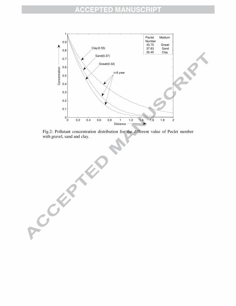
For many practical problems related to solute transport in groundwater, the
advection term usually dominates. To measure the degree of advection domination, a
dimensionless Peclet number is commonly used. Physically, the Peclet number
measures the relative magnitude of advection versus dispersion. Low Peclet numbers
imply that the solute transport is dominated by the dispersion process. High Peclet
numbers imply that advection is the dominant process controlling solute transport.
Generally, the non dimensional Peclet number is defined as the ratio of the advective

and dispersive component of solute transport with the small spatial variation in space
i.e., 0
0
u xPe
nD= .
The Peclet number varies with the porosity of the different geological
formations can also be discussed. For a large Peclet number, this does not
significantly affect the overall mass transport rate, which is the combination of
convection and dispersion. The first-type boundary condition or Dirichlet type
boundary condition, however, does have an effect on the solute transport rate for a
smaller Peclet number. From Figure 2, we have been observed that the Peclet number
is higher with lower the porosity and therefore, pollutant concentration level increases
by reducing the Peclet number at each of the positions. The pollutant concentration is
decreasing with distance and reaches to the minimum values tending to zero.
From Figure 3, we have been observed that the pollutant concentration for
different Peclet numbers in clay medium increases with increasing time periods at
each of the positions and starts decreasing with distance and reducing approximately
up to zero concentration. Due to highly advective systems (high Peclet numbers), the
pollutant concentration increases with increasing time period. However, in case of
highly dispersive systems (small Peclet numbers), it appears that the source of
pollutants having less impact and it reduces to minimum concentration in compare of
large peclet number. So, the solute concentration increases with increasing the value
of Peclet number.
Similarly, in case of courant number the pollutant concentration distribution is
also predicted for the different geological formations. It has been predict for uniform
time dependent input source concentration. Therefore, the corresponding effect of the
non-dimensional parameters like courant number defined as the ratio of the advective
terms to the distance with time variation in the medium. Mathematically, it defined in

terms of the porosity as 0r
u tC
nX= . Figure 4, shows that the pollutant concentration in
the different medium with the different courant numbers in a particular time. The
courant number increases with decreasing the value of the averaging porosity. The
nature of the pollutant concentration is depicted and observed that concentration
values increases by reducing the courant number at each of the position. These
concentration values are decreasing with distance and reached approximately up to
zero concentration.
The pollutant concentration pattern has also been predicted for the different
medium such as aquifer and aquitard and shown in Figure 5. The solute concentration
increases with increasing the porosity but in both the medium solute concentration
starts decreasing with respect to the distance and reaches up to minimum values of
concentration. The concentration values increases with respect to time at each of the
positions. This reveals for the exponentially increasing type unsteady velocity pattern.
Analytical solution for Cauchy type boundary condition given in equation (28)
has been computed with the same set of data taken into consideration as discussed in
the analytical solution for Dirichlet type boundary problem given in equation (24)
except 0 7.0(km/year), 0.02u λ= = in the domain 0 1.0x≤ ≤ (km). Due to the regular
human activity on the earth surface, the seepage velocity of the solute increases with
respect to the time and therefore the concentration pattern has been depicted for
exponentially decreasing seepage velocity in case of the Cauchy type boundary
condition. The distribution pattern for the exponential decreasing type of the velocity
expression is depicted in the Figure 6, for the different geological formations with
their average porosity in 6th, 7th and 8th year respectively. It is observed that the
pollutant concentration increases in the aquitard (clay) in compare to the aquifer
(gravel) at each of the positions. The pollutant source increases with respect to time

but the concentration decreases with distance in the both the formations. The pollutant
concentration pattern for the different value of the peclet number for the different
medium with same time period has been depicted and shown in the Figure 7. It is
observed that the solute concentration increases with decreasing the value of the
peclet number with their averaging porosity at each of the positions. The decreasing
trend has also been observed with distance and attains its minimum concentration.
The solute concentration pattern decreases with increasing the value of the courant
number for the different medium with their averaging porosity at each of the positions
and shown in the Figure 8.
Figure 9 (a), 9(b) and 9(c) provides the decreasing trend of correlation between Peclet
and courant number for three different geological formations with their averaging
porosity. It can also be observed that the correlation becomes nonlinear as the
averaging porosity increases.
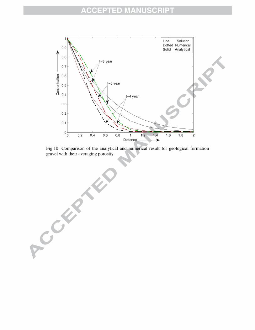
Figures 10 depicts that the comparison between numerical solution (dotted line) and
analytical solution (solid line) for exponentially decreasing form of velocity pattern in
the gravel medium. We observe that the concentration distribution pattern is almost
similar in both the solutions and having a very good agreement which validate the
result. However, Figure (11) depicts that the same for gravel, sand and clay for fixed
time i.e., 6 years. In both the results, pollutant concentration for the clay (i.e.,
aquitard) is high as compared to the gravel and sand (i.e., aquifer). Since the
transmission rate is low in aquitard as compare to the aquifer so the level of pollutant
is high for the sort time period in aquitard, after that is remains the uniform nature
with respect to the distance. As the averaging porosity level increases the pollutant
concentration also increases and ultimately both the pattern goes to its minimum
concentration which observed from the Figure (11). From these figures we observed

that the pollutant concentration initially increases for numerical approximation and
after covering some distance it takes the decreasing nature as compare to the
analytical solution. Figures 12 to 14, depicts the pollutant concentration profile for
increasing pulse type boundary condition into the gravel, sand and clay medium
respectively. The level of pollutant concentration is increases for numerical result as
compare to the analytical one and it takes reverse pattern after covering some distance
for gravel medium shown in the Figure12. In case of the sand and clay medium the
level of pollutant increases in analytical result as compare to the numerical one. The
level of pollutant is slightly increased for short distances in the case of the numerical
result of the sand medium with their averaging porosity shown in the Figure 13. The
level of the pollutant concentration is very low in the case of the clay medium for the
numerical result shown in the Figure 14. These changes may happen due to structure
of geological formations taken into consideration in this study.
In the numerical solution, different numbers of grid points have been used. Selecting
the different number of grid points reveals that mesh size can affect the accuracy of
the results. To confirm the validity of the results, they are compared with the
analytical solution results. In this paper, the R.M.S. error has also been calculated
from the pollutant concentration values obtained from the analytical and the
numerical solution for the advection dispersion equation. R.M.S. error has been used
to measured the performance of numerical result against the analytical one. The two
parameters in numerical methods i.e., z∆ and *T∆ which are necessary to investigate
the effect of their respective changes under the stability condition given in equation
(39). So, numerical investigation has been made for execution of R.M.S. error and
their corresponding CPU time shown in Table 1 for Dirichlet type boundary condition
with z∆ =0.2, 0.3, 0.4, * 0.001T∆ = and time duration is 4 year. However, the same

has been executed shown in Table 2 for the mixed type boundary condition with
z∆ =0.2, 0.5, 0.7, * 0.001T∆ = and time duration is 6 year. The R.M.S. error increases
with increasing the value of z∆ and therefore, the result is more accurate for the small
value of z∆ which can be observed from Table1. From Table 2 we observed that the
result is more accurate for the large values of z∆ may be due to mixed type of
boundary condition in which concentration gradient is taken into account. So, it may
now be concluded that the numerical results obtained from explicit finite difference
method are very close to the analytical results. R.M.S. error indicates the accuracy of
the result obtained. However, in most of the cases it is necessary to maintain a desired
accuracy while keeping the CPU time as minimum as possible. It has been observed
from Table 1 and Table 2 that the CPU time in the problem of mixed type boundary
condition is more than the Dirichlet type boundary condition.
6. Summary and Conclusions
In our present work, an analytical study of scale dependent solute dispersion
with linear isotherm in heterogeneous medium has been discussed and compared with
numerical solution. The non reactive solute transport in an aquifer-aquitard system
has been studied with Dirichlet and Cauchy type boundary conditions. Advection,
dispersion, zero-order production term, and linear adsorption have been included. The
governing equations of solute transport in the solid liquid phases simultaneously are
solved analytically by Laplace integral transform technique, and analytical solutions
are then subsequently inverted numerically/ graphically in the real time domain. The
solution derived may be applicable for regions near the persisting pollutant sources
(or far from the moving fronts of the pollutant source). Some of the findings from this
study can be summarized as follows:
� The effects of non-dimensional parameters i.e., Peclet number and Courant
number over pollutant concentration have been explored in the various geological
formations with their averaging porosity.
� The kinetic nature of the solute transport into the groundwater flow predicted for
the different geological formation. The pollutant concentration Pattern is high in
the aquitard (clay) in compare to the aquifer (gravel).
� The correlation relation between Peclet and Courant number becomes non linear
as the value of the averaging porosity increases.
� Exponentially decreasing and increasing forms of time dependent unsteady
velocity patterns have been used.
� Very good agreement has been found between analytical and numerical solution.
� Accuracy of the solution has also been obtained using root mean square error
analysis.
Acknowledgments
The authors are thankful to Indian School of Mines, Dhanbad for providing financial
support to Ph.D. candidate under the ISMJRF scheme. The authors are also thankful
to the Editor and Reviewers comments which helped to improve the quality of paper.
References
Aral, M. M., Liao, B., 1996. Analytical solutions for two-dimensional transport
equation with time-dependent dispersion coefficients. J. Hydrol. Eng. 1(1), 20-
32.
Ataie-Ashtiani, B.,Hosseini, S.A., 2005. Numerical errors of explicit finite difference
approximation for two-dimensional solute transport equation with linear sorption.
Environm. Modelli. & Soft. 20, 817-826.

Ataie-Ashtiani, B., Lockington, D.A., Volker, R.E., 1999. Truncation errors in finite
difference models for solute transport equation with first-order reaction. J.
Contam. Hydrol. 35 (4), 409-428.
Bakker, M., 1999. Simulating groundwater flow in multi-aquifer systems with
analytical and numerical Dupuit-models. J. Hydrol., 222, 55-64.
Batu, V., 1989. A generalized two-dimensional analytical solution for hydrodynamic
dispersion in bounded media with the first-type boundary condition at the source.
Water Resour. Res., 25(6), 1125-1132.
Batu, V., 1993. A generalized two-dimensional analytical solute transport models in
bounded media for flux-type multiple sources. Water Resour. Res., 29(8), 2881-
2892.
Bear, J., 1972. Dynamics of fluids in porous media, American Elsevier,New York.
Bruce, J. C., Street, R. L.,1967. Studies of free surface flow and two dimensional
dispersion in porous media. Report no.63, Civil Eng. Dept. Stanford Univ.
Stanford, California.
Chen, J.S., Ni, C.F., Liang, C.P., Chiang, C.C., 2008. Analytical power series solution
for contaminant transport with hyperbolic asymptotic distance-dependent
dispersivity. J. Hydrol. 362, 142-149.
Chen, J.S., Liu, C.W., 2011. Generalized analytical solution for advection-dispersion
equation in finite spatial domain with arbitrary time-dependent inlet boundary
condition. Hydrol. Earth Syst. Sci., 15, 2471–2479.
Chen, J.S., Lai K. H., Liu, C.W., Ni, C.F., 2012. A novel method for analytically
solving multi-species advective-dispersive transport equations sequentially
coupled with first-order decay reactions. J. Hydrol. 420-421,191-204.
Davit, Y., Wood, B. D., Debenest, G., Quintard, M., 2012. Correspondence Between
One- and Two- Equation Models for Solute Transport in Two-Region
Heterogeneous Porous Media. Transp. Porous Med. 95. 213-238.
Delay, F., Porel, G., De Marsily, G., 1997. Predicting solute transport in
heterogeneous media from results obtained in homogeneous ones: an
experimental approach. J. Contami. Hydrol., 25, 63-84.
Deng B., Li, J., Zhang , B., Li ,N., 2014. Integral transform solution for solute
transport in multi-layered porous media with the implicit treatment of the
interface conditions and arbitrary boundary conditions. J. Hydrol. 517, 566-573.
Diaw, E.B., Lehmann, F., Ackerer, Ph., 2001. One-dimensional simulation of solute
transfer in saturated-unsaturated porous media using the discontinuous finite
elements method. J. Contam. Hydrol. 51(3-4), 197-213.
Du, R., Cao, W.R., Sun, Z.Z., 2010. A compact difference scheme for the fractional
Diffusion-wave equation. Appli. Mathema. Modell. 34(10), 2998-3007.
Ebach, E.H., White, R., 1958. Mixing of fluids flowing through beds of packed solids.
Trans. America. Insti. Chem. Eng. 4(2), 161-169.
Fahs, M., Younes, A., Mara, T.A., 2014. A new benchmark semi-analytical solution
for density-driven flow in porous media. Advances in Water Resources 70, 24–
35.
Freeze, R.A., Cherry, J.A., 1979. Groundwater. Prentice-Hall, Englewood Cliffs, New
Jersey.
Gao, G., Zhan, H., Feng, S., Fu, B., Huang, G., 2012. A mobile-immobile model with
an asymptotic scale-dependent dispersion function. J. Hydrol. 424-425,172-183.
Guerrero, J.S. P., Pimentel, L.C.G., Skaggs, T.H., van Genuchten M.Th.,2009.
Analytical solution of the advection–diffusion transport equation using a change-

of-variable and integral transform technique. Inter. J. Heat and Mass Trans. 52,
3297-3304.
Guerrero, J.S.P., Skaggs, T.H., 2010. Analytical solution for one-dimensional
advection–dispersion transport equation with distance-dependent coefficients. J.
Hydrol. 390, 57-65.
Guerrero, J.S.P., Pontedeiro, E.M., van Genuchten, M.Th, Skaggs, T.H., 2013.
Analytical solutions of the one dimensional advection-dispersion solute transport
equation subject to time-dependent boundary condition. Chemic. Eng. J.
221,487-491.
Hayek, M., 2011. Exact and traveling-wave solutions for convection–diffusion–
reaction equation with power-law nonlinearity. Applied Mathematics and
Computation. 218, 2407–2420.
Huang, G., Huang, Q., Zhan, H., 2006. Evidence of one-dimensional scale-dependent
fractional advection-dispersion. J. contami. hydrol. 85, 53-71.
Huang, Q., Huang, G., Zhan, H., 2008. A finite element solution for the fractional
advection-dispersion equation. Adv. in Water Resour. 31, 1578-1589.
Hoopes, J.A., Harleman, D.R.F., 1965. Waste water recharge and dispersion in porous
media, MIT Hydrodynamics Lab Report No. 75. Cambridge, Massachusetts.
Hunt, B. 1978. Dispersion sources in uniform groundwater flow. J. Hydraul.
Div.,104(HY1), pp.75–85.
Kim, S., Kavvas, M.L., 2006. Generalized fick’s law and fractional ADE for pollution
transport in river: detailed derivation. J. Hydrol. Eng. 11(1), 80-83.
Kumar, N., 1983. Dispersion of pollutant in semi-infinite porous media with unsteady
velocity distribution. Nordic Hydrol. 14(3),167-178.

Kumar, N., 1983. Unsteady flow against dispersion in finite porous media. J. Hydrol.
63, 345-358.
Lantz, R.B., 1971. Quantitative evaluation of numerical diffusion truncation error.
Society Petroleum Engineering Journal 11,315-320.
Lee, T.C., 1999. Applied Mathematics in Hydrogeology. Lewis Publishers, Boca
Raton.
Liu C., Ball W. P., HughEllis J., 1998. An Analytical Solution to the One-
Dimensional Solute Advection-Dispersion Equation in Multi-Layer Porous
Media. Transp.in Porous Med. 30, 25-43.
Liu, H.H., Zhang, Y.Q., Zhou Q., Molz, F.J., 2007. An interpretation of potential
scale dependence of the effective matrix diffusion coefficient. J. Contami.
Hydrol. 90, 41–57.
Maraqa M. A., Khashan, S. A., 2014. Modeling solute transport affected by
heterogeneous sorption kinetics using single-rate non equilibrium approaches. J.
Contami. Hydrol.157,73–86.
Marino, M. A., 1974. Longitudinal dispersion in saturated porous media. J. Hydraul.
Div., ASCE. 101(HY1), 151-157.
McKenna, S. A., Walker, D. D., Arnold B., 2003. Modeling dispersion in three-
dimensional heterogeneous fractured media at Yucca Mountain. J. Contam.
Hydrol.,62-63, 577-594.
Mickley H. S., Sherwood T. K., Reed C.E., 1957. Applied Mathematics in Chemical
Engineering. McGraw-Hill, New York.

Notodarmojo, S., Ho, G.E., Scott, W.D., Davis, G.B., 1991. Modelling phosphorus
transport in soils and groundwater with two-consecutive reactions. Water Res. 25
(10), 1205-1216.
Ogata, A. and Banks, R. B. 1961. A solution of the differential equation of
longitudinal dispersion in porous media. Fluid movement in earth materials.
Geological survey professional paper 411-A, United States.
Ptak, T., Piepenbrink, M., Martac E., 2004. Tracer tests for the investigation of
heterogeneous porous media and stochastic modelling of flow and transport-a
review of some recent developments. J. Hydrol. 294, 122–163.
Roberts, D. L., Selim, M. S., 1984. Comparative study of six explicit and two
implicit finite difference schemes for solving one-dimensional parabolic partial
differential equations. Int. J. Numer. Methods Eng.,20,817-844.
Roubinet, D., De Dreuzy, J. R., Tartakovsky, D.M., 2012. Semi-analytical solutions
for solute transport and exchange in fractured porous media. Water Resour. Res.
48, w01542, doi:10.1029/2011wr011168.
Ranganathan, P., Farajzadeh R., Bruining H., Zitha, P.L.J., 2012. Numerical
simulation of natural convection in heterogeneous porous media for CO2
geological storage. Transp. Porous Med. 95, 25–54.
Saied, E., Khalifa, M.E., 2002. Some analytical solutions for groundwater flow and
transport equation. Transp. porous Media. 47, 295-308.
Schafer, W., Kinzelbach, W.K.H., 1996. Transport of reactive species in
heterogeneous porous media. J. Hydrol., 183, 151-168 .
Singh, M. K., Kumari, P., 2014, Contaminant concentration prediction along unsteady
groundwater flow. Modelling and Simulation of Diffusive Processes, XII, 257-
276. DOI: 10.1007/978-3-319-05657-9.

Singh, P., Yadav S. K., Kumar, N., 2012. One-dimensional pollutant’s advective-
diffusive transport from a varying pulse-type point source through a medium of
linear heterogeneity. J. Hydrol. Eng. 17(9), 1047-1052.
Serrano, S.E., 1995. Forecasting scale-dependent dispersion from spills in
heterogeneous aquifers. J. of Hydrol.169,151-169.
Smith, G.D., 1978. Numerical Solution of Partial Differential Equations: Finite
Difference Methods, second ed. Oxford University Press, Oxford.
Verma, A.K., Bhallamudi, S.M., Eswaran, V.,2000. Overlapping Control Volume
Method for Solute Transport. J. Hydrol. Eng. 5(3), 308-316.
Vasquez C., Ortiz C., Suarez F., Munoz J. F., 2013.Modeling flow and reactive
transport to explain mineral zoning in the Atacama salt flat aquifer, Chile. .J.
Hydrol. 490,114-125.
van Genuchten, M.Th., Leij, F. J., Skaggs, T. H., Toride,N., Bradford, S. A.,
Pontedeiro, E. M., 2013. Exact analytical solutions for contaminant transport in
rivers 1. The equilibrium advection-dispersion equation. J. Hydrol. Hydromech.,
61(2),146–160.
Wang, S. T., McMillan, A.F., Chen, B. H.,1978. Dispersion of pollutants in channels
with non-uniform velocity distribution. Water Res. 12(6),389-394.
You, K., Zhan, H., 2013. New solutions for solute transport in a finite column with
distance-dependent dispersivities and time-dependent solute sources. J. Hydrol.
487, 87-97.
Zheng, C., Bennett, G.D., 2002. Applied Contaminant Transport Modeling, second
ed. Wiley, New York.

Zoppou, C., Knight, J.H., 1997. Analytical Solution for Advection and Advection-
Diffusion Equations with Spatially Variable Coefficients. J. Hydraul. Eng.,
ASCE, 123(2), 144-148.

0 0.2 0.4 0.6 0.8 1 1.2 1.4 1.6 1.8 20
0.1
0.2
0.3
0.4
0.5
0.6
0.7
0.8
0.9
1
Distance
Concentr
ation
Medium(n) Line
Gravel(0.32) Dotted
Clay(0.55) Solid
t=8 year
t=6 year
t=4 year
Fig.1: Pollutant concentration distribution for the different geological formations
gravel and clay with their averaging porosity.
0 0.2 0.4 0.6 0.8 1 1.2 1.4 1.6 1.8 20
0.1
0.2
0.3
0.4
0.5
0.6
0.7
0.8
0.9
1
Distance
Co
nce
ntr
ati
on
t=8 year
Peclet Medium
Number
43.75 Gravel
37.83 Sand
25.45 Clay
Sand(0.37)
Gravel(0.32)
Clay(0.55)
Fig.2: Pollutant concentration distribution for the different value of Peclet number with gravel, sand and clay.

0 0.2 0.4 0.6 0.8 1 1.2 1.4 1.6 1.8 20
0.1
0.2
0.3
0.4
0.5
0.6
0.7
0.8
0.9
1
Distance
Conce
ntr
ation
Peclet Line
Number
25.45 Solid
18.18 Dotted
t=8 year
t=6 year
t=4 year
Fig.3: Pollutant concentration distribution for the different value of the Peclet number
for the clay medium.

0 0.2 0.4 0.6 0.8 1 1.2 1.4 1.6 1.8 20
0.1
0.2
0.3
0.4
0.5
0.6
0.7
0.8
0.9
1
Distance
Conc
entr
ati
on
Courant Medium
Number
4.37 Gravel
3.78 Sand
2.54 ClayClay(0.55)
Sand(0.37)
Gravel(0.32)
t=4 year
Fig.4: Pollutant concentration distribution for the different value of the Courant number with gravel, sand and clay

0 0.2 0.4 0.6 0.8 1 1.2 1.4 1.6 1.8 20
0.1
0.2
0.3
0.4
0.5
0.6
0.7
0.8
0.9
1
Distance
Conc
entr
ati
on
t=6 year
Medium(n) Line
Gravel(0.32) Solid
Clay(0.55) Dotted
t=8 year
t=4 year
Fig.5: Pollutant concentration distribution for exponentially increasing velocity pattern

0 0.1 0.2 0.3 0.4 0.5 0.6 0.7 0.8 0.9 10
0.5
1
1.5
2
2.5
3
3.5
4
4.5
5
Distance
Co
ncen
tratio
n
t=8 year
t=7 year
t=6 year
Medium Line
Gravel(0.32) Dotted
Clay(0.55) Solid
Fig.6: Pollutant concentration distribution of the increasing pulse type input source

0 0.1 0.2 0.3 0.4 0.5 0.6 0.7 0.8 0.9 10
0.5
1
1.5
2
2.5
3
3.5
Distance
Co
ncen
tra
tion
Peclet Medium
Number
218.75 Gravel
189.18 Sand
127.25 Clay
Gravel(0.32)
Sand(0.37)
Clay(0.55)
t=6 year
Fig.7: Pollutant concentration distribution for the increasing pulse type source for the
different value of Peclet number.

0 0.1 0.2 0.3 0.4 0.5 0.6 0.7 0.8 0.9 10
0.5
1
1.5
2
2.5
3
3.5
4
4.5
Distance
Concentr
ation
Courant Medium
Number
153.12 Gravel
132.43 Sand
89.09 ClayClay(0.55)
Sand(0.37)
Gravel(0.32) t=7 year
Fig.8: Pollutant concentration distribution for the increasing pulse type source for
different value of Courant number.

4 6 8 1015
20
25
30
35
40
Cr
Pe
Sand medium
Fig. 9(a) Fig. 9(b)
3 4 5 6 710
15
20
25
30
Cr
Pe
Clay medium
Fig. 9(c)
Fig.9 Correlation between the Peclet number and Courant number for (a) gravel (b)
sand and (c) clay
4 6 8 10 1220
25
30
35
40
45
Cr
Pe
Gravel medium
0 0.2 0.4 0.6 0.8 1 1.2 1.4 1.6 1.8 20
0.1
0.2
0.3
0.4
0.5
0.6
0.7
0.8
0.9
1
Distance
Concentr
ation
t=6 year
t=8 year
t=4 year
Line Solution
Dotted Numerical
Solid Analytical
Fig.10: Comparison of the analytical and numerical result for geological formation
gravel with their averaging porosity.

0 0.2 0.4 0.6 0.8 1 1.2 1.4 1.6 1.8 20
0.1
0.2
0.3
0.4
0.5
0.6
0.7
0.8
0.9
1
Distance
Concentr
ation Gravel (0.32)
Sand (0.37)
Clay (0.55)
Line Solution
Dotted Numerical
Solid Analytical
Fig.11: Comparison of the analytical and numerical result for the different geological formations with their averaging porosity for fixed time 6 years.

0 0.2 0.4 0.6 0.8 1 1.2 1.4 1.6 1.8 20
0.1
0.2
0.3
0.4
0.5
0.6
0.7
0.8
0.9
Distance
Concentr
ation
t=6 year
Line Solution
Dotted Numerical
Solid Analytical
Fig.12: Comparison of the analytical and numerical result for the gravel geological formation with their averaging porosity for increasing plus type source.

0 0.2 0.4 0.6 0.8 1 1.2 1.4 1.6 1.8 20
0.1
0.2
0.3
0.4
0.5
0.6
0.7
0.8
0.9
1
Distance
Concentr
ation
Line Solution
Dotted Numerical
Solid Analytical
t=6 year
Fig.13: Comparison for the analytical and numerical result for the sand geological
formation with their averaging porosity for increasing plus type source.

0 0.2 0.4 0.6 0.8 1 1.2 1.4 1.6 1.8 20
0.5
1
1.5
2
2.5
3
3.5
Distance
Concentr
ation
t=6 year
Line Solution
Dotted Numerical
Solid Analytical
Fig.14: Comparison for the analytical and numerical result for the clay geological
formation with their averaging porosity for increasing plus type source.

Figure Captions:
Fig.1: Pollutant concentration distribution for the different geological formations
gravel and clay with their averaging porosity.
Fig.2: Pollutant concentration distribution for the different value of Peclet number
with gravel, sand and clay.
Fig.3: Pollutant concentration distribution for the different value of the Peclet number
for the clay medium.
Fig.4: Pollutant concentration distribution for the different value of the courant
number with gravel, sand and clay.
Fig.5: Pollutant concentration distribution for exponentially increasing velocity
pattern.
Fig.6: Pollutant concentration distribution of the increasing pulse type input source.
Fig.7: Pollutant concentration distribution for the increasing pulse type source for the
different value of Peclet number.
Fig.8: Pollutant concentration distribution for the increasing pulse type source for
different value of Courant number.
Fig.9: Correlation between the Peclet number and Courant number for (a) gravel (b)
sand and (c) clay
Fig.10: Comparison of the analytical and numerical result for geological formation
gravel with their averaging porosity.
Fig.11: Comparison of the analytical and numerical result for the different geological
formations with their averaging porosity for fixed time 6 years.
Fig.12: Comparison of the analytical and numerical result for the gravel geological
formation with their averaging porosity for increasing plus type source.

Fig.13: Comparison for the analytical and numerical result for the sand geological
formation with their averaging porosity for increasing plus type source.
Fig.14: Comparison for the analytical and numerical result for the clay geological
formation with their averaging porosity for increasing plus type source.

Table-1: R.M.S. Error for the dirichlet type boundary condition with time 4years
Distance Analytical
Result
Numerical Result
0.2z∆ = 0.3z∆ = 0.4z∆ =
0.2 0.6322 0.7158 0.5053 0.3491
0.6 0.1897 0.1031 0.0214 0.0109
1.0 0.0399 0.0100 0.0087 0.0090
1.4 0.0111 0.0086 0.0090 0.0095
1.8 0.0072 0.0088 0.0094 0.1000
R.M.S. 0.0554 0.0953 0.1503
CPU Time (sec) 12.37 17.64 17.50 16.86

Table-2: R.M.S. Error for the mixed type boundary condition with 6 years
Distance Analytical
Result
Numerical Result
0.2z∆ = 0.5z∆ = 0.7z∆ =
0.2 0.3596 0.7222 0.4779 0.3265
0.6 0.1898 0.4205 0.0430 0.0060
1.0 0.1151 0.1884 0.0006 0.0001
1.4 0.0763 0.0581 0.0001 0.0001
1.8 0.0537 0.0084 0.0001 0.0001
R.M.S. 0.1961 0.1070 0.1065
CPUTime (sec) 12.58 21.16 21.71 20.96

Highlights of the paper
1. Scale dependent solute dispersion with linear isotherm
2. One-dimensional analytical solution in heterogeneous medium with Dirichlet
and Cauchy type boundary conditions
3. Solute Concentration with Peclet and Courant numbers in different geological
formations i.e., Clay, gravel and sand
4. Comparison of analytical solution with numerical one
5. Accuracy of the solution with mean square error analysis


