© 2012 Kavita Bala •(with previous instructors James/Marschner)
Cornell CS4620/5620 Fall 2012 • Lecture 26 1
CS4620/5620: Lecture 26
Sampling and Anti-Aliasing
© 2012 Kavita Bala •(with previous instructors James/Marschner)
Cornell CS4620/5620 Fall 2012 • Lecture 26
Announcements
• 4621 – Next two Fridays
• Friday, Nov 2 (splines), Nov 9 (animation)
2
© 2012 Kavita Bala •(with previous instructors James/Marschner)
Cornell CS4620/5620 Fall 2012 • Lecture 26
Antialiasing
• Point sampling makes an all-or-nothing choice in each pixel– therefore steps are inevitable when the choice changes– discontinuities are bad
• On bitmap devices this is necessary– hence high resolutions required– 600+ dpi in laser printers to make aliasing invisible
• On continuous-tone devices we can do better
3
© 2012 Kavita Bala •(with previous instructors James/Marschner)
Cornell CS4620/5620 Fall 2012 • Lecture 26
Antialiasing and resampling
• Antialiasing by regular supersampling is the same as rendering a larger image and then resampling it to a smaller size
• So we can re-think this– one way: we’re computing area of pixel covered by primitive– another way: we’re computing average color of pixel
• this way generalizes easily to arbitrary filters, arbitrary images
4
© 2012 Kavita Bala •(with previous instructors James/Marschner)
Cornell CS4620/5620 Fall 2012 • Lecture 26
Weighted filtering
• Box filtering problem– Treats area near edge same as area near center
• results in pixel turning on “too abruptly”
• Alternative: weight area by a smoother filter– unweighted averaging corresponds to using a box function
5
© 2012 Kavita Bala •(with previous instructors James/Marschner)
Cornell CS4620/5620 Fall 2012 • Lecture 26
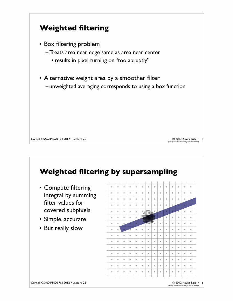
Weighted filtering by supersampling
• Compute filtering integral by summing filter values for covered subpixels
• Simple, accurate• But really slow
6

© 2012 Kavita Bala •(with previous instructors James/Marschner)
Cornell CS4620/5620 Fall 2012 • Lecture 26
Gaussian filteringin action
7
© 2012 Kavita Bala •(with previous instructors James/Marschner)
Cornell CS4620/5620 Fall 2012 • Lecture 26
Filter comparison
Point sampling Box filtering Gaussian filtering
8
© 2012 Kavita Bala •(with previous instructors James/Marschner)
Cornell CS4620/5620 Fall 2012 • Lecture 26
Sampling Theory
9
© 2012 Kavita Bala •(with previous instructors James/Marschner)
Cornell CS4620/5620 Fall 2012 • Lecture 26
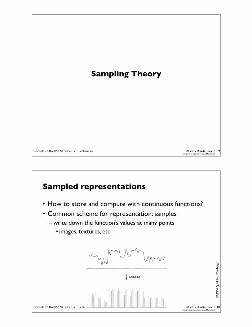
Sampled representations
• How to store and compute with continuous functions?• Common scheme for representation: samples
– write down the function’s values at many points• images, textures, etc.
[FvD
FH fi
g.14
.14b
/ W
olbe
rg]
10

© 2012 Kavita Bala •(with previous instructors James/Marschner)
Cornell CS4620/5620 Fall 2012 • Lecture 26
Reconstruction
• Making samples back into a continuous function– for output (need realizable method)– for analysis or processing (need mathematical method)– amounts to “guessing” what the function did in between
[FvD
FH fi
g.14
.14b
/ W
olbe
rg]
11
© 2012 Kavita Bala •(with previous instructors James/Marschner)
Cornell CS4620/5620 Fall 2012 • Lecture 26
Roots of sampling
• Nyquist 1928; Shannon 1949– famous results in information theory
• 1940s: first practical uses in telecommunications• 1960s: first digital audio systems• 1970s: commercialization of digital audio• 1982: introduction of the Compact Disc
– the first high-profile consumer application
• This is why all the terminology has a communications or audio “flavor”– early applications are 1D; for us 2D (images) is important
12

© 2012 Kavita Bala •(with previous instructors James/Marschner)
Cornell CS4620/5620 Fall 2012 • Lecture 26
Sampling in digital audio
• Recording: sound to analog to samples to disc• Playback: disc to samples to analog to sound again
– how can we be sure we are filling in the gaps correctly?
13
© 2012 Kavita Bala •(with previous instructors James/Marschner)
Cornell CS4620/5620 Fall 2012 • Lecture 26
What is aliasing?
• What if we “missed” things between the samples?• Simple example: undersampling a sine wave
– unsurprising result: information is lost– surprising result: indistinguishable from lower frequency– also was always indistinguishable from higher frequencies– aliasing: signals “traveling in disguise” as other frequencies
14

© 2012 Kavita Bala •(with previous instructors James/Marschner)
Cornell CS4620/5620 Fall 2012 • Lecture 26
Preventing aliasing
• Introduce lowpass filters:– remove high frequencies leaving only safe, low frequencies– choose lowest frequency in reconstruction (disambiguate)
15
© 2012 Kavita Bala •(with previous instructors James/Marschner)
Cornell CS4620/5620 Fall 2012 • Lecture 26
Filtering
• Processing done on a function– can be executed in continuous form (e.g. analog circuit)– but can also be executed using sampled representation
• Simple example: smoothing by averaging
16

© 2012 Kavita Bala •(with previous instructors James/Marschner)
Cornell CS4620/5620 Fall 2012 • Lecture 26
Linear filtering: a key idea
• Transformations on signals; e.g.:– blurring/sharpening operations in image editing– smoothing/noise reduction in tracking
• Can be modeled mathematically by convolution
17
© 2012 Kavita Bala •(with previous instructors James/Marschner)
Cornell CS4620/5620 Fall 2012 • Lecture 26
Convolution warm-up
• basic idea: define a new function by averaging over a sliding window
• a simple example to start off: smoothing
18

© 2012 Kavita Bala •(with previous instructors James/Marschner)
Cornell CS4620/5620 Fall 2012 • Lecture 26
Convolution warm-up
• Same moving average operation, expressed mathematically:
19
© 2012 Kavita Bala •(with previous instructors James/Marschner)
Cornell CS4620/5620 Fall 2012 • Lecture 26
Discrete convolution
• Simple averaging:
– every sample gets the same weight
• Convolution: same idea but with weighted average
– each sample gets its own weight (normally zero far away)
• This is all convolution is: it is a moving weighted average
20

© 2012 Kavita Bala •(with previous instructors James/Marschner)
Cornell CS4620/5620 Fall 2012 • Lecture 26
Filters
• Sequence of weights a[j] is called a filter• Filter is nonzero over its region of support
– usually centered on zero: support radius r
• Filter is normalized so that it sums to 1.0– this makes for a weighted average, not just any
old weighted sum
• Most filters are symmetric about 0– since for images we usually want to treat
left and right the same
a box !lter
21
© 2012 Kavita Bala •(with previous instructors James/Marschner)
Cornell CS4620/5620 Fall 2012 • Lecture 26
Convolution and filtering
• Can express sliding average as convolution with a box filter
• abox = […, 0, 1, 1, 1, 1, 1, 0, …]
22

© 2012 Kavita Bala •(with previous instructors James/Marschner)
Cornell CS4620/5620 Fall 2012 • Lecture 26
Example: box and step
23
© 2012 Kavita Bala •(with previous instructors James/Marschner)
Cornell CS4620/5620 Fall 2012 • Lecture 26
Convolution and filtering
• Convolution applies with any sequence of weights• Example: Bell curve (Gaussian-like) […, 1, 4, 6, 4, 1, …]/16
24

© 2012 Kavita Bala •(with previous instructors James/Marschner)
Cornell CS4620/5620 Fall 2012 • Lecture 26
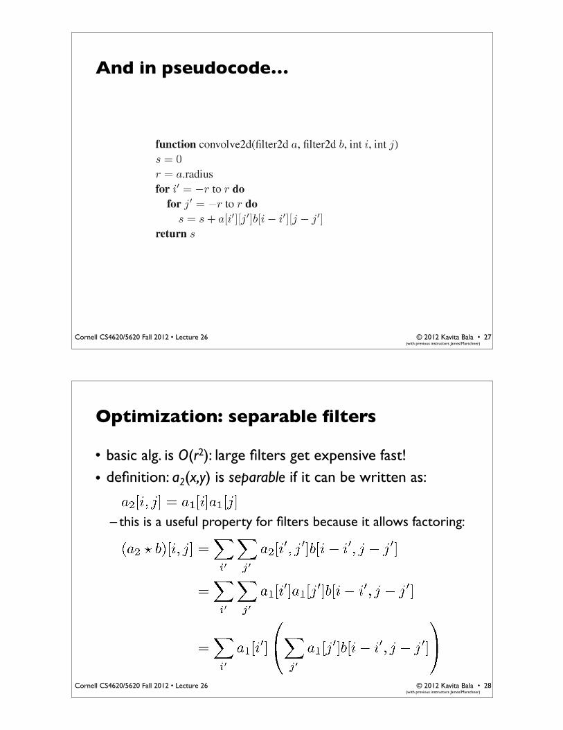
And in pseudocode…
25
© 2012 Kavita Bala •(with previous instructors James/Marschner)
Cornell CS4620/5620 Fall 2012 • Lecture 26
Discrete filtering in 2D
• Same equation, one more index
– now the filter is a rectangle you slide around over a grid of numbers
• Commonly applied to images– blurring (using box, gaussian, …)– sharpening
• Usefulness of associativity– often apply several filters one after another: (((a * b1) * b2) * b3)
– this is equivalent to applying one filter: a * (b1 * b2 * b3)
26
© 2012 Kavita Bala •(with previous instructors James/Marschner)
Cornell CS4620/5620 Fall 2012 • Lecture 26
And in pseudocode…
27
© 2012 Kavita Bala •(with previous instructors James/Marschner)
Cornell CS4620/5620 Fall 2012 • Lecture 26
Optimization: separable filters
• basic alg. is O(r2): large filters get expensive fast!
• definition: a2(x,y) is separable if it can be written as:
– this is a useful property for filters because it allows factoring:
28

© 2012 Kavita Bala •(with previous instructors James/Marschner)
Cornell CS4620/5620 Fall 2012 • Lecture 26
two-stage resampling using aseparable !lter
[Phi
lip G
reen
spun
]
29
© 2012 Kavita Bala •(with previous instructors James/Marschner)
Cornell CS4620/5620 Fall 2012 • Lecture 26
Continuous convolution
• Can apply sliding-window average to a continuous function just as well– output is continuous– integration replaces summation
30
© 2012 Kavita Bala •(with previous instructors James/Marschner)
Cornell CS4620/5620 Fall 2012 • Lecture 26
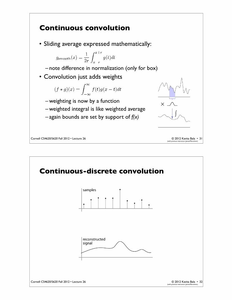
Continuous convolution
• Sliding average expressed mathematically:
– note difference in normalization (only for box)
• Convolution just adds weights
– weighting is now by a function– weighted integral is like weighted average– again bounds are set by support of f(x)
31
© 2012 Kavita Bala •(with previous instructors James/Marschner)
Cornell CS4620/5620 Fall 2012 • Lecture 26
Continuous-discrete convolution
32
© 2012 Kavita Bala •(with previous instructors James/Marschner)
Cornell CS4620/5620 Fall 2012 • Lecture 26
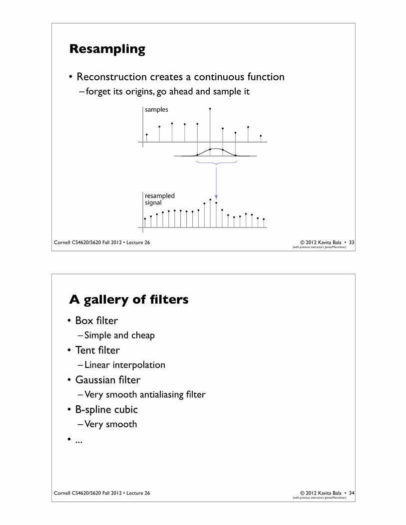
Resampling
• Reconstruction creates a continuous function– forget its origins, go ahead and sample it
33
© 2012 Kavita Bala •(with previous instructors James/Marschner)
Cornell CS4620/5620 Fall 2012 • Lecture 26
A gallery of filters
• Box filter– Simple and cheap
• Tent filter– Linear interpolation
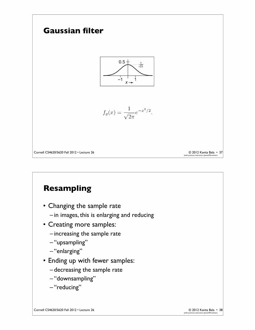
• Gaussian filter– Very smooth antialiasing filter
• B-spline cubic– Very smooth
• ...
34

© 2012 Kavita Bala •(with previous instructors James/Marschner)
Cornell CS4620/5620 Fall 2012 • Lecture 26
Box filter
35
© 2012 Kavita Bala •(with previous instructors James/Marschner)
Cornell CS4620/5620 Fall 2012 • Lecture 26
Tent filter
36
© 2012 Kavita Bala •(with previous instructors James/Marschner)
Cornell CS4620/5620 Fall 2012 • Lecture 26
Gaussian filter
37
© 2012 Kavita Bala •(with previous instructors James/Marschner)
Cornell CS4620/5620 Fall 2012 • Lecture 26
Resampling
• Changing the sample rate– in images, this is enlarging and reducing
• Creating more samples:– increasing the sample rate– “upsampling”– “enlarging”
• Ending up with fewer samples:– decreasing the sample rate– “downsampling”– “reducing”
38

© 2012 Kavita Bala •(with previous instructors James/Marschner)
Cornell CS4620/5620 Fall 2012 • Lecture 26
Reducing and enlarging
• Very common operation– devices have differing resolutions– applications have different memory/quality tradeoffs
• Also very commonly done poorly• Simple approach: drop/replicate pixels• Correct approach: use resampling
39
© 2012 Kavita Bala •(with previous instructors James/Marschner)
Cornell CS4620/5620 Fall 2012 • Lecture 26
1000 pixel width [Philip Greenspun]
40

© 2012 Kavita Bala •(with previous instructors James/Marschner)
Cornell CS4620/5620 Fall 2012 • Lecture 26
250 pixel width
by dropping pixels gaussian !lter
[Philip Greenspun]
41
© 2012 Kavita Bala •(with previous instructors James/Marschner)
Cornell CS4620/5620 Fall 2012 • Lecture 26
4000 pixel width
box reconstruction !lter bicubic reconstruction !lter
[Phi
lip G
reen
spun
]
42
© 2012 Kavita Bala •(with previous instructors James/Marschner)
Cornell CS4620/5620 Fall 2012 • Lecture 26
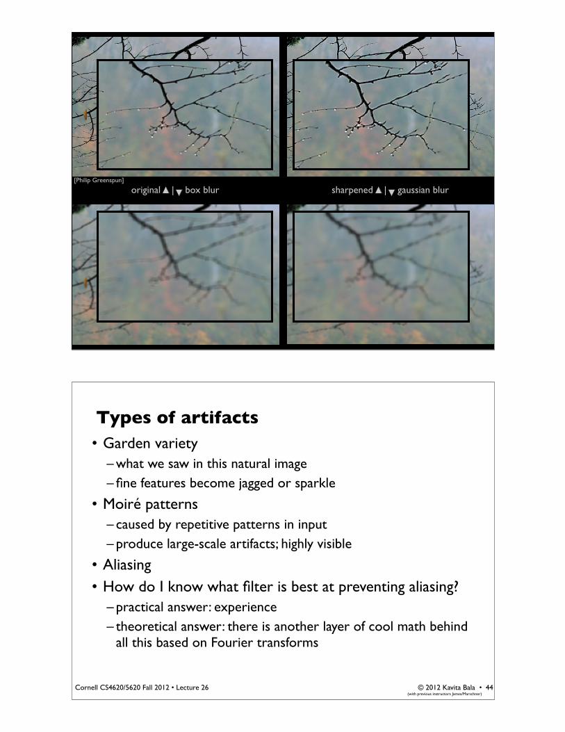
original | box blur sharpened | gaussian blur[Philip Greenspun]
© 2012 Kavita Bala •(with previous instructors James/Marschner)
Cornell CS4620/5620 Fall 2012 • Lecture 26
Types of artifacts• Garden variety
– what we saw in this natural image– fine features become jagged or sparkle
• Moiré patterns– caused by repetitive patterns in input– produce large-scale artifacts; highly visible
• Aliasing• How do I know what filter is best at preventing aliasing?
– practical answer: experience– theoretical answer: there is another layer of cool math behind
all this based on Fourier transforms
44

© 2012 Kavita Bala •(with previous instructors James/Marschner)
Cornell CS4620/5620 Fall 2012 • Lecture 26
Again: Weighted filtering for line drawing
• Box filtering problem: treats area near edge same as area near center– results in pixel turning on “too abruptly”
• Alternative: weight area by a smoother filter– unweighted averaging corresponds to using a box function– sharp edges mean high frequencies
• so want a filter with good extinction for higher freqs.– a Gaussian is a popular choice of smooth filter– important property: normalization (unit integral)
45
© 2012 Kavita Bala •(with previous instructors James/Marschner)
Cornell CS4620/5620 Fall 2012 • Lecture 26
Weighted filtering by supersampling
• Compute filtering integral by summing filter values for covered subpixels
• Simple, accurate• But really slow
46
© 2012 Kavita Bala •(with previous instructors James/Marschner)
Cornell CS4620/5620 Fall 2012 • Lecture 26
Gaussian filteringin action
47
© 2012 Kavita Bala •(with previous instructors James/Marschner)
Cornell CS4620/5620 Fall 2012 • Lecture 26
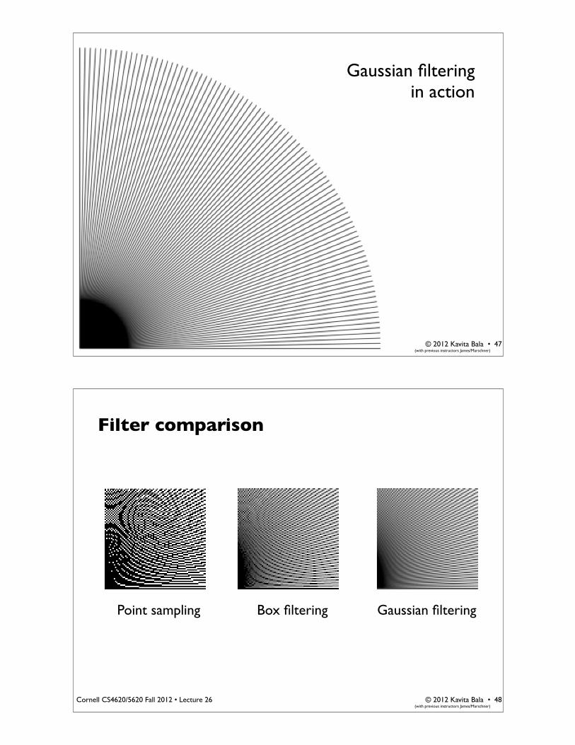
Filter comparison
Point sampling Box filtering Gaussian filtering
48


