
Research Collection
Report
Performance characterization and modeling of the molecularsimulation code opal
Author(s): Arbenz, Peter; Stricker, Thomas M.; Taufer, Michela; Matt, Urs von
Publication Date: 1998
Permanent Link: https://doi.org/10.3929/ethz-a-006653085
Rights / License: In Copyright - Non-Commercial Use Permitted
This page was generated automatically upon download from the ETH Zurich Research Collection. For moreinformation please consult the Terms of use.
ETH Library

Performance Characterization and Modeling of the Molecular
Simulation Code Opal
Peter Arbenz1 and Thomas Stricker1 and Michela Taufer1 and Urs von Matt2
1Departement of Computer Science 2 Integrated Systems Engineering AG (ISE)
ETH Zuerich, Zentrum 111 North Market Street
CH-8092 Zuerich, Switzerland San Jose, CA 95113, USAemail: arbenz,stricker,[email protected] email: [email protected]
December 1, 1998
Abstract
In modern parallel computing there exists a large number of highly different platforms and it is im-
portant to choose the right parallel platform for a computationally intensive code. To decide about the
most cost effective parallel platform, a computer scientist needs a precise characterization of the appli-
cation properties, such as memory usage, computation and communication requirements. The computer
architects need this information to provide the community with new, more cost effective platforms. The
precise resource usage is of little interest to the users or computational scientists in the applied field, so
most traditional parallel codes are ill equipped to collect data about their resource usage and behavior at
run time. Once an application runs, is numerically stable and there is some speedup, most computational
scientists declare victory and move on to the next application. Contrary to that philosophy, our group
of computer architects invested a considerable amount of effort and time to instrument Opal, a paral-
lel molecular biology simulation code, for an accurate performance characterization on a given parallel
platform. As a result we can present a simple analytical model for the execution time of that particular
application code along with an in depth verification of that model through measured execution times.
The model and measurements can not only be used for performance tuning but also for a good prediction
of the code’s performance on alternative platforms, like newer and cheaper parallel architectures or the
next generation of supercomputers to be installed at our site.
1 Introduction
Molecular dynamics simulation is a powerful and widespread computational tool used in many fields of
chemistry and biology. In molecular dynamics, the simulation task is to solve the classical equations of
motion for the change of a molecular system over the time. While conceptually simple, the molecular
dynamics simulation is computationally demanding. In theory, molecular dynamics simulation application
could run on a large number of highly different computing platforms in parallel and vectorized computing.
The use of massively parallel platforms adds new aspects to the layout of computation and to its performance
analysis: the speed of memory and processors are no longer the sole factors to consider, but also the speed
of interprocessor communication needs to be taken into account.
1
Many other investigations have recently been devoted to the development of fast and efficient algorithms for
molecular dynamics simulation, but not enough attention has been paid to the choice of the best suited and
most cost effective parallel computer as a target platform for the simulation code. Today, most scientists
just use the computer they have available locally or the supercomputer at the computation center they have
easy access to. In a world of global networking and rapidly falling prices for tremendous power in personal
computing this is no longer adequate. However, to find better machines is difficult, since parallel codes are ill
equipped to collect data about their resource usage and behavior at run time and the corresponding data are
rarely published and even more rarely related to other published performance data. In many publications,
the scientists just give long lists of measured times without any critical analysis or any reference to the
application features.
In our previous work [21] we followed the past, traditional approach to develop a fast and efficient parallel
algorithm for Opal, a molecular biology application developed locally at the Institute of Molecular Biology
and Biophysics at the ETH Zurich. The parallel version of Opal has become similar to Amber [7]: not
only both the codes do energy minimization and molecular dynamics, but, both codes use lists of molecular
components, which need to be updated periodically, and which allow to evaluate the interactions of each
component with a limited part of the molecular complex by means of a cut-off distance. In that part of
our work we have paid a lot of attention to the algorithm of parallelization, while we kept the performance
analysis at the minimum and restricted ourself to simple measurements of the execution time.
As an improvement over the current state of the art in the field of scientific computation, we propose and
demonstrate in this report an integrated approach to design, parallelization and performance analysis of Opal
using a combination of modeling and measurements. This approach is the result of a thorough investigation
which has shown how the most codes do not offer any performance publication, but just lists of bench-
marking measured, e.g. Amber [9, 8], without any reference to critical aspects of the codes or possible
improvements.
Besides a detailed assessment of performance achieved on the reference platform, a Cray J90, the primary
goal of our study is to find the most suitable and most cost effective hardware platform for the application,
in particular to check its suitability for fast CoPs, SMP CoPs and slow CoPs, three flavors of Clusters of
Pentium PCs, built by our computer architecture group. As a result we present a simple analytical model
for the execution time of Opal with an in depth model verification through measured execution times. The
model and measurements are not only used for performance tuning, but also for a good prediction of the
code’s performance on these alternative platforms. The full overlap of computation and communication
in the initial parallel version of Opal hid many latency mechanisms. We introduce synchronization tools,
PVM barriers, which eliminate overlap of the communication and computation but at the same time allow to
gather accurate and detailed performance measurements of every execution time components separately. The
new measurements show the importance of the communication overhead, which have not been considered
sufficiently during the earlier parallelization attempts.
In Chapter 2, we give a brief overview on the application program Opal and its parallelization. Moreover,
we describe the parallel computers which run Opal and the main features of the communication middle-ware
packages used (Sciddle and PVM). In Chapter 3, we discuss the experimental design as well as how we solve
the measurement problems encountered in the determination of the execution time of Opal. In Chapter 4,
we develop a simple analytical model to help with the prediction of the performance of Opal and to give
immediate answers about the performance on different platforms. In Chapter 5, we show the measured
2

performance of Opal on a Cray J90 and hereby verify the analytical model against an actual implementation.
Finally, in Chapter 6, we investigate the performance prediction of Opal for alternative platforms using the
analytical model, while, in Chapter 7, we draw conclusions and discuss some implications of our results.
2 Background
We start this section with an overview of the application program Opal and the main aspects of its paral-
lelization [21, 1]. We will explain the main features of the Sciddle middle-ware package for communication
and PVM, as well as the architectural characteristics of the experimental unit on which the application will
run, the Cray J90, an installation of four vector SMPs at the ETH Zurich.
2.1 Opal Package
Opal is a software package to perform energy minimizations and molecular dynamics simulations of proteins
and nucleic acids in vacuum or in water [18]. Opal uses classical mechanics, i.e., the Newtonian equations
of motion, to compute the trajectories�ri�t� of n atoms as a function of time t. Newton’s second law expresses
the acceleration as:
mid2
dt2�ri�t� � �Fi�t�� (1)
where mi denotes the mass of atom i. The force �Fi�t� can be written as the negative gradient of the atomic
interaction function V :�Fi�t� � �
∂∂�ri�t�
V ��r1�t�� � � ���rn�t���
A typical function V has the form:
V ��r1� � � ���rn� � ∑allbonds
12
Kb�b�b0�2� ∑
allbondangles
12
KΘ�θ�θ0�2�
∑improperdihedrals
12
Kξ�ξ�ξ0�2� ∑
dihedrals
Kϕ�1�cos�nϕ�δ���
∑allpairs�i� j�
�C12�i� j�
r12i j
�C6�i� j�
r6i j
�qiq j
4πε0εrri j
��
The first term models the covalent bond-stretching interaction along bond b. The value of b0 denotes the
minimum-energy bond length, and the force constant Kb depends on the particular type of bond. The second
term represents the bond-angle bending (three-body) interaction. The (four-body) dihedral-angle interac-
tions consist of two terms: a harmonic term for dihedral angles ξ that are not allowed to make transitions,
e.g., dihedral angles within aromatic rings or dihedral angles to maintain chirality, and a sinusoidal term for
the other dihedral angles ϕ, which may make 360� turns. The last term captures the non-bonded interactions
over all pairs of atoms. It is composed of the van der Waals and the Coulomb interactions between atoms i
and j with charges qi and q j at a distance ri j.
2.1.1 Opal-2.6
A first version of Opal, Opal-2.6, was developed at the Institute of Molecular Biology and Biophysics
at ETH Zurich [17]. It was written in standard FORTRAN-77 and optimized for vector supercomputers
3
through a few vectorizable loops. The code of Opal-2.6 is sequential in the sense that a single processor
runs the whole computation. Opal-2.6 spends most of its computing time during a simulation evaluating
the non-bonded interactions over all pairs of atoms of the molecular system (the last term of the atomic
interaction function V ). Fortunately, these calculations also offer a high degree of parallelism in addition to
the vectorizable inner loops.
2.1.2 Parallel Opal
The parallel version of Opal [21, 1] distributes the evaluation of the non-bonded interactions among multiple
processors in a client-server setting.
A single client coordinates the work and performs the following tasks:
� runs the main program,
� manages the user interactions,
� executes the sequential fraction of the program (the numerical integration the differential equations),
� computes of the bonded interactions.
Multiple servers deal with the computation that contribute most of the work to the total computation. They
perform the following task in parallel:
� compute the Van der Waals and Coulomb forces making up for non-bonded interactions.
With a slight change of the molecular simulation model, i.e.,the use of water molecules as single units
centered in the oxygen atoms in the solvent instead of three individual atoms, we accomplished:
� a reduced workload for the servers,
� a reduction in size of the memory usage,
� an increase in accuracy for the molecular energy calculations when reduced parts of the molecular
complex are considered.
In reference to this model change, we will often use the term mass center to label either a single atom of the
protein or the nucleic acid or a single water molecules of the solvent.
For a molecular complex 1 of n atoms, the number of non-bonded interactions between atoms, which must be
evaluated, is of the order of n2. In the new version of Opal, the complexity of the molecular energy evaluation
can be reduced by omitting many of the non-bonded interactions from the molecular energy computation. At
first, the data describing the non-bonding interaction parameters between the solute-solute, solute-solvent,
solvent-solvent atoms are replicated on all the servers. This global information, whose volume depends
on the problem size and does not scale with the number of processors, allows each server to compute
independently. With its copy of global data, each server runs its simulation tasks requesting no further
parameters from the client except for the atom coordinates.
The simulation consists of a repetitive computation task that terminates with the display of information about
the total energy, the volume, the pressure and the temperature of the molecular complex. In the first stage of
1A molecular complex is the combination of a solute such as proteins or nucleic acids and a solvent, e.g. water.
4

each simulation step, called update phase, each server selects a distinct subset of mass center pairs, checks
their distance and adds the pair to its own list of all active pairs when the mass centers are not beyond the
given distance cut-off. In the second stage of the simulation step, the servers compute partial non-bonded
energy components (Van der Waals energy and Coulomb energy) using the list of all active pairs. When a
mass center is an oxygen atom, representing a water molecule, the server expands it into three atoms (one
oxygen and two hydrogens), and computes the non-bonded interaction force for each of them. At the end of
this step each server sends its partial results to the client which gathers them and sums the total molecular
energy of the molecular complex as well as its volume, pressure and temperature.
The data in each list is updated periodically. The interval between successive updates can be selected by the
user through the setting of an Opal parameter called update. The value of the update parameter expresses
the number of interaction steps after which the lists of all active pairs are updated. Every 1�update iteration
steps the distance of the mass center i from the mass center j is calculated, for all pairs �i� j�, 1� i� j � nc,
where nc is the number of mass centers. If the mass center i is further than cut-off away from mass center j
then their interaction is neglected. It is not known in advance which pairs �i� j� have to be taken into account
and, in a parallel computation, it is therefore not known how the load is distributed among the processors.
It must be assumed that the mass center data are input in a somewhat regular way with respect to geometry.
Therefore, there is the danger that the work among processors is unevenly distributed if the pairs �i� j� are
distributed in a regular fashion, e.g., in blocks of consecutive i-values. Hence, we proceeded in the following
way. The mass center indices i � 1� � � � �nc are randomly permuted by a permutation π [19, p. 63]. The
random number generator used was proposed by Knuth [16, p. 170]. The index pair �i� j� is then dealt with
by processor π�i� mod p where p is the number of processors. The permutation π is stored in an array of
length nc of which each processor generates its own list of mass centers independently. We could not handle
the random permutation of all the nc�nc�1��2 index pairs simultaneously as this would have consumed too
much memory. As π just permutes the set f1� � � ��ncg the distribution of indices on the processors is as even
as possible. It thus seems reasonable to expect also the work load to be well balanced among the processors.
We tailored the parallelization of the code to the hardware platform on which Opal runs. The use of list
structures could introduce indirect addressing and potential data dependences. These two factors do not
allow a complete vectorization of all the inner loops (the loops which are candidates for vectorization) and
reduce the performance of Opal on vector supercomputers, like the Cray J90. To get rid of non-vectorizable
code fragments we rewrote the code and the list data structures in a way to avoid non-vectorizable data
dependences. A high degree of vectorization was achieved through compiler directives after this rewrite.
2.2 PVM and Sciddle Systems
The client server structure of Opal is ideally suited for a remote procedure call (RPC) system. We used
Sciddle [3, 2], an RPC system extension to the PVM [13] communication library. Sciddle2 consists of
a stub generator (Sciddle compiler) and a run-time library. The stub generator reads the remote interface
specification, i.e., the description of the subroutines exported by the servers, and generates the corresponding
communication stubs. The stubs take care of translating an RPC into the necessary PVM message passing
primitives. The application does not need to use PVM directly during an RPC: the client simply calls a
2Sciddle is public domain software. It may be downloaded from the Sciddle home page at
http://www.scsc.ethz.ch/www/pub/Sciddle/Sciddle.html.
5

subroutine (provided by the client stub), and the Sciddle run-time system invokes the corresponding server
subroutine (via the server stub). It was, however, a deliberate decision in Sciddle to use PVM directly for
process management (starting and terminating of servers). Thus a Sciddle application still needs to use a
few PVM calls at the beginning and the end of a run.
Sciddle was designed to support parallel applications through asynchronous RPCs. An asynchronous RPC
is split into an invoke part and a claim part. This avoids the need for threads in the client, as it is required in
other RPC systems (e.g., OSF DCE [10]). Thus Sciddle is a highly portable communication library. It has
been ported to Linux PCs, UNIX workstations, the Intel Paragon, and supercomputers like the Cray J90 and
the NEC SX-4. In particular, Sciddle supports both PVM systems on the Cray J90, the network PVM and
the shared memory PVM.
The benchmark tests in [2] show that the overhead of Sciddle for a typical application is very small. As we
will see later this is also the case for Opal. Furthermore the safety and ease of use of an RPC system turned
out to be a major benefit in the development of the parallel version of Opal.
2.3 The Architecture of the Cray J90 SuperCluster
Our tests are conducted on a set of four Cray J90s that form a SMP Cluster at ETH Zurich. Figure 1 shows
the layout of the machines in question. Experimentation with all four symmetric multiprocessor (SMP) as a
cluster was initially planned but abandoned because of the poorly understood overhead in the communication
software and therefore the Hippi communication infrastructure remained unused. Our primary platform is a
single J90 SMP. It is a symmetric multiprocessor system built from eight processors with efficient sequential
and vector processing capacities (10 ns cycle), large memory (2048 MB), high memory bandwidth and
efficient I/O capabilities (2 x HIPPI).
M M M M M M
M M MMMM
P P P
P PP P P P
I/O I/O
I/OI/O
P P P
ETH back-bone
512 Memory banks
512 Memory banks 512 Memory banks
8 Processors
8 Processors 8 Processors
16 Processors
HIPPI-Switch ES-1
FDDI Netzwerk
1024 Memory banks
Figure 1: Layout of the Cray J90 at ETH.
6

3 Problem Design
In this chapter we describe the set of experiments used to characterize the performance of Opal simulation
and we outline solutions to some measurement problems for the determination of the execution time of Opal.
3.1 Experimental Design
At first, we specify the variables that affect the responses of the experiments (factors), the value that they
can assume (levels), the outcome of the experiments (response variable) and the number of replications of
each experiment.
3.1.1 Choice of the Factors
Table 1 shows the factors that we consider in our experiments and their levels, the values that they can
assume.
Factor Levels
1 Number of servers p 1,2,3,4,5,6,7
2 Size of the problem n medium problem size, large problem size
3 Cut-off parameter c with cut-off, no cut-off
4 Update parameter u full update, partial update
Table 1: The test cases.
We consider four factors and we determine their relative importance:
Factor 1: Number of servers
The number of servers, which run the energy contribution of the non-bonded interactions, ranges from
one to seven.
Factor 2: Size of the Problem
Two different molecular complexes are investigated. A first test suite consists of a simulation of a
medium size molecular complex (medium problem): the complex between the Antennapedia home-
odomain from Drosophila and DNA [5, 11], composed by 1575 atoms and immersed in 2714 water
molecules (4289 mass centers). The total number of atoms n, i.e., the molecular atoms and the atoms
of solvent, is 9715. In a second test, we consider the simulation of a large size molecular complex
(large problem): the NMR structure of the LFB homeodomain, composed by 1655 atoms and im-
mersed in 4634 water molecules (6289 mass centers). The total number of atoms n is 15557.
7
Factor 3: Cut-off Parameter
Two different orders of computation complexities are examined for every molecular complex. In a
first simulation, all the non-bonded interactions among the n atoms of the molecular complex are
taken into account. A non-effective cut-off parameter of 60 A is considered (no cut-off ). The compu-
tation complexity grows quadratic with the problem size. In a second simulation, an effective cut-off
parameter of 10 A (with cut-off ) has been chosen. Only a small part of the non-bonded interactions
among the n atoms of the molecular complex are considered and the overall computation complexity
grows linearly with the problem size.
Factor 4: Update Parameter
We investigate the role of the update parameter on the performance. Two different cases are consid-
ered: a full update case, in which each step of the simulation provides the update of the lists, and a
partial update case, in which the lists are updated each ten iteraction steps.
3.1.2 Full Factorial Design
We choose a full factorial experimental design according to the framework presenteded in [15] to character-
ize the computational efficiency of Opal. A full factorial design utilizes every possible combination of the
factors in Table 1. The number of the experiments is:
�7 servers� � �2 problem sizes� � �2 cut-off values� � �2 update values� � 56 experiments
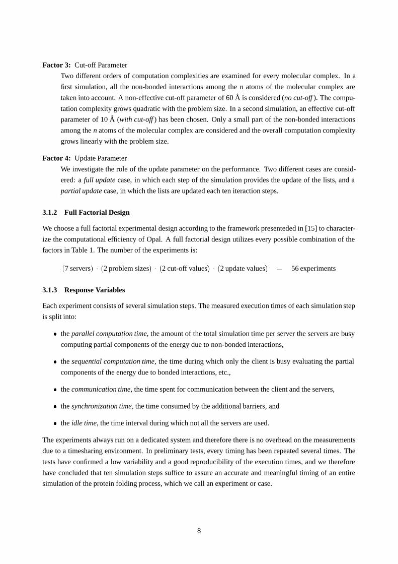
3.1.3 Response Variables
Each experiment consists of several simulation steps. The measured execution times of each simulation step
is split into:
� the parallel computation time, the amount of the total simulation time per server the servers are busy
computing partial components of the energy due to non-bonded interactions,
� the sequential computation time, the time during which only the client is busy evaluating the partial
components of the energy due to bonded interactions, etc.,
� the communication time, the time spent for communication between the client and the servers,
� the synchronization time, the time consumed by the additional barriers, and
� the idle time, the time interval during which not all the servers are used.
The experiments always run on a dedicated system and therefore there is no overhead on the measurements
due to a timesharing environment. In preliminary tests, every timing has been repeated several times. The
tests have confirmed a low variability and a good reproducibility of the execution times, and we therefore
have concluded that ten simulation steps suffice to assure an accurate and meaningful timing of an entire
simulation of the protein folding process, which we call an experiment or case.
8

3.2 Synchronization Tools
In a parallel system many tasks run at the same time. A high overlap of computation and communication
appears desirable to improve efficiency. Most parallelization tools, like Sciddle [22], support and encourage
this overlap of computation and communication. The major problem with middleware tools like Sciddle is
that they provide no support for a detailed quantification and correct accounting of the elapsed time for local
computation, communication and idle waits that occur due to load imbalance. For a precise and complete
analysis of the performance of Opal, a more precise timing model must be adopted. Such a model defines
the most important timing intervals, which are in our case the computation time of the servers (parallel
computation time), their idle time, the communication time between client and servers, as well as the time
in which only the client runs (sequential computation time). To allow the measurements of these metrics,
we need to give up some overlap and introduce new synchronization tools in Sciddle. These tools separate
the communication times properly from the computation times.
3.2.1 Instrumentation for our performance characterization
In a pure Sciddle environment, it might be easy to measure and accumulate high level metrics like server
computation rate, client computation rate, but low level indicators like communication efficiency, idle times,
and load imbalance are much harder to get. The latter metrics are most relevant to the performance analysis.
At first we show the difficulties to measure and quantify overhead in Sciddle and propose a modification to
the timing synchronization behavior to address this problem. Figure 2 shows an execution time line of an
original Sciddle run when two servers are called by the client and all three processes run in parallel. By
comparing client and server computation times, this execution model admits to estimate the fraction of the
time in which each single server is busy servicing requests (parallel computation time) and the correspond-
ing time the client is busy servicing the server calls (sequential computation time). The two numbers can
only indicate that performance is bad and not why performance is bad.
Interesting metrics like the idle time, defined as the period during which a server is not used, and the com-
munication time, defined as the interval between a client request and a server response and vice versa, are
harder to measure, but highly useful for performance studies.
With only a few changes to the Sciddle communication environment and in particular with the introduction
of additional barriers, it is possible to measure or compute all these metrics directly. The barrier function
lets the servers synchronize themselves explicitly with each other. Figure 3 shows a time line of a modified
Sciddle run with two servers and two barriers.
A call of the function call barrier A locks the servers- and the client- run until all the processes have
called the function: when this occurs, the servers and the client are released and the servers process the
remote procedure call. The interval between the client’s requests and the release of all the processes is
defined as the call time. At the end of an RPC, each server provides its computation time and calls the
function barrier B. This starts a new block during which the idle time of the server is measured. When
all the processes have called the barrier function, barrier B, they start the communication phase with the
client waiting until the servers have processed their RPC’s and the results are returned. This new mode of
synchronization changes the overall execution time slightly.
The use of a shared communication channel between servers and client introduces contention due to limited
network resources at the end of a client computation phase. This contention is application specific and it is
9

SERVER 1
SERVER 2
call invoke_S1
call invoke_S2
call claim_S1
call claim_S2
CLIENT
clie
nt c
ompu
tatio
n tim
e (s
erve
r 1)
clie
nt c
ompu
tatio
n tim
e (s
erve
r 2)
server com
putation time (server 1)
server com
putation time (server 2)
Figure 2: Pure client-server model.
likely with the unmodified version of Sciddle when all the servers perform exactly the same amount of work
(without large servers idle time values). The barriers in the modified Sciddle run just expose the contention
in all cases.
3.2.2 Integration of barriers into Sciddle
The Sciddle environment does not provide explicit synchronization tools, but it allows a direct communica-
tion with the underlying PVM environment and therefore permits explicit synchronization.
Figure 4 shows the hierarchy of Opal, Sciddle, and PVM. In order to allow the synchronization of the
processes we use the barrier tools from PVM, i.e., PVMBARRIER ([13]), which lets the Opal tasks explicitly
synchronize with each other.
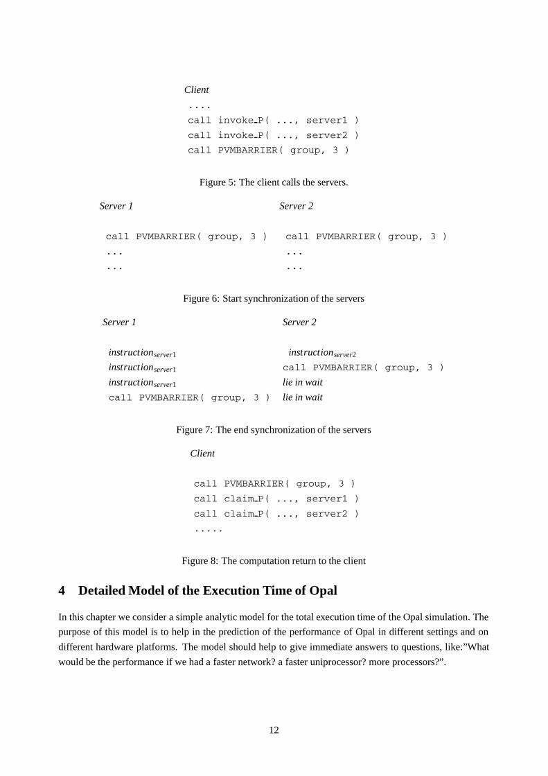
For a better understanding of PVM, we give a brief example for the situation already considered in our time
line graph in in Figure 3. Two servers are called by a single client. The client calls sequentially both servers
using the normal Sciddle tools and finishes the call phase by invoking the PVM function PVMBARRIER
(see Figure 5). As soon as an RPC is invoked, a relative server calls the PVM function PVMBARRIER, (see
Figure 6). The barrier causes a wait state for all the tasks until exactly all processors in the group reach the
barrier and are released. At this point of the simulation all servers start simultaneously with their part of the
computation while the client enters its new wait phase by calling the PVM functionPVMBARRIER a second
time (see Figure 8). It remains in a blocked state until all the servers have finished their computation and
10

server com
p. time
(server 1)
server com
p. time
(server 2)
idle tim
e
SERVER 1
SERVER 2
call invoke_S1
call barrier_A
call invoke_S2
call barrier_B
call
time
S1
call
time
S2
call claim_S1
call claim_S2 re
turn
time
S2
retu
rn
time
S1
CLIENT
Figure 3: The client-server model with barriers.
Opal
Sciddle
PVM
Hardware
Drivers
Middleware
Application
Figure 4: Software hierarchy of the Opal implementation, based on Sciddle and PVM.
have called the PVM function PVMBARRIER again (see Figure 7). As soon as the client is released from
the barrier it starts the claim phase. The client gathers the partial results of the computation from the servers
using the Sciddle toolbox routine claim P (see Figure 8).
11
Client
....
call invoke P( ..., server1 )
call invoke P( ..., server2 )
call PVMBARRIER( group, 3 )
Figure 5: The client calls the servers.
Server 1 Server 2
call PVMBARRIER( group, 3 ) call PVMBARRIER( group, 3 )
... ...
... ...
Figure 6: Start synchronization of the servers
Server 1 Server 2
instructionserver1 instructionserver2
instructionserver1 call PVMBARRIER( group, 3 )
instructionserver1 lie in wait
call PVMBARRIER( group, 3 ) lie in wait
Figure 7: The end synchronization of the servers
Client
call PVMBARRIER( group, 3 )
call claim P( ..., server1 )
call claim P( ..., server2 )
.....
Figure 8: The computation return to the client
4 Detailed Model of the Execution Time of Opal
In this chapter we consider a simple analytic model for the total execution time of the Opal simulation. The
purpose of this model is to help in the prediction of the performance of Opal in different settings and on
different hardware platforms. The model should help to give immediate answers to questions, like:”What
would be the performance if we had a faster network? a faster uniprocessor? more processors?”.
12

4.1 Factors of the Model
In this section we present the analytic model of Opal. We have paid particular attention to develop a simple
model capable of capturing the essential parameters of the real application. A set of factors, that affect the
outcome of the timing experiment, is used to predict the response (i.e., execution times):
s : number of simulation steps,
p : number of servers,
n : size of the problem, i.e., the number of atoms of the whole molecular complex,
u : update parameter, 0 � u � 1, indicating the frequency of the lists update,
c : cut-off parameter, expressed in A,
d : molecular density, the average number of atoms per unit volume. We assume it to be uniform and
constant during the simulation.
In order to simplify the analytical model of Opal, we combine the cut-off parameter and the density of
the molecular complex scalability into a single factor, n. This factor represents the average number of
neighboring atoms that contribute to the non-bonded interactions with a given atom:
n �43
π c3d (2)
4.2 Model for the total execution time
The execution time of Opal, tOpal , can be split in four terms:
tOpal � ttot par comp � ttot seq comp � ttot comm � ttot sync (3)
where:
� ttot comm, the total communication time, is the time spent in the communication.
� ttot par comp, the total parallel computation time, is the computation time spent by the servers servicing
requests.
� ttot seq comp, the total sequential computation time, is the total time spent by the client to compute the
values of energy, pressure, volume, and temperature within the molecular complex from the partial
energy and force components computed in the parallel phase.
� ttot sync, total synchronization time, is the time to synchronize the processes with each other.
4.2.1 Parallel Computation Time: ttot par comp
The total parallel computation time, ttot par comp, is the amount of the total simulation time the servers are
busy servicing requests. It is the sum of the maximum time spent by the servers to run the update routine
13

tupdate3, and the maximum time spent by the servers to run the energy evaluation routine tnbint
4.
ttot par comp � tupdate� tnbint (4)
As the number of servers increases, the work in the update routine and in the energy evaluation routine is
distributed among more processors: tupdate as well as tnbint decrease as p increases. Further, tupdate depends
linearly on the update parameter u.
The time spent during the whole simulation to run the update routine t update always grows quadratic with
the number of mass centers because whenever the servers update their own list, all the pairs of mass centers
must be checked. At the same time, the update time decreases linearly with the increase of the time interval
between two list updates. tupdate can be approximated as:
tupdate�na�nm�� a2s up
�na�nm� �na�nm�1�2
(5)
where na is the number of atoms of the protein or nuclei acid, nm is the number of water molecules, and a2
represents the time for:
� generating a pair of atoms,
� checking their distance.
The term:�na�nm� �na�nm�1�
2represents the total number of mass center pairs that are generated and whose distance is checked during the
update routine.5 Let us define the new parameter γ as the ratio of the number of water molecules, nm, and
the total number of atoms, n. Then:
nm � γ n (6)
na � �1�3 γ� n (7)
and tupdate becomes:
tupdate�n�� a2s up
�1�2 γ�2 n2� �1�2 γ� n2
(8)
When the simulation takes place in vacuum, the number of water molecules, nm, is null and tupdate changes
into:
tupdate�n�0�� a2sup
n2�n2
(9)
At the same time, the time tnbint spent in the energy evaluation routine is subject to the effects of the cut-
off parameter: the dimension of the lists, on which pairs the partial energy values are evaluated, increases
drastically with the increase of the cut-off distance. The energy-evaluation routine grows quadratic up to the
number atoms within the cut-off radius and linear beyond that. tnbint can be approximated by:
tnbint�n� n��
�a3
sp
n�n�1�2 when n� n
a3sp n n when n� n
(10)
3The update routine updates the lists of mass center pairs4The energy evaluation routine evaluates the partial energy values of the non-bonded interactions (Van der Waals energy and
Coulomb energy)5Each water molecule is considered as one unit centered in the oxygen atom instead of three individual atoms.
14

a3 is the time needed to compute the Van der Waals energy and Coulomb energy, of a single pair of atoms.
For n � n, the energy contribution of the non-bonded interactions are evaluated for all the atoms of the
molecular complex. When a component of a pair in a mass center list is a oxygen atom representing a
water molecule, the server expands it into three atoms (one oxygen and two hydrogens), and computes the
interaction force for each of them. The energy evaluation entirely dominates the parallel computation time:
tnbint �� tupdate
The term:n�n�1�
2represents the total number of pairs of atoms considered. The computational effort of the computation
becomes a quadratic polynomial in n.
Otherwise, with the introduction of the cut-off parameter, the amount of the computation for n � n in the
energy evaluation routine is reduced drastically: many of the non-bonded interactions are omitted from the
energy evaluation. For each atom of the molecular complex, only a constant number of neighboring atoms
(n) contributes to the energy values of the non-bonded interactions. The amount of pairs of atom considered
in this case becomes:
n n
with n a constant determined by a cut-off; so the energy computation time becomes a linear polynomial in n.
Despite its lower asymptotic complexity due to the introduction of a cut-off parameter, the energy evaluation
routine still dominates the update process in this second case for all practical problem sizes. The crossover
point for which the update time equals the energy evaluation time depends on the molecular complex volume
as well as the cut-off parameter. For our simulations (see Chapter 5) crossover happens for unrealistically
high numbers of water molecules or protein atoms. Furthermore, there is the option of a decrease of the
update frequency, and with it the fraction of update computation can be reduced arbitrarily to restore the
relation of:
tnbint � tupdate
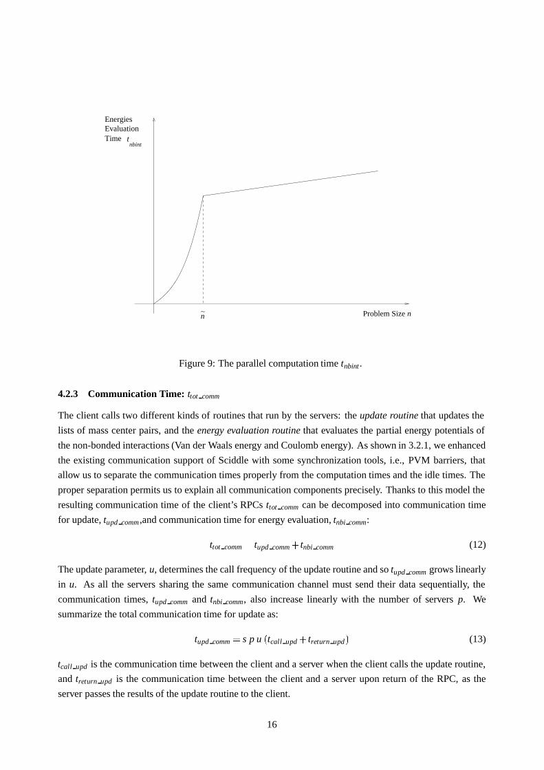
Figure 9 explains the behavior of tnbint�n� n�, as n varies from 0 to ∞ with n arbitrarily fixed.
Finally, the total parallel computation time is summarized in equation (4) by:
ttot par comp �
�����
s2 p �a2 u �1�2 γ�2�a3� n2� s
2 p �a2 u �1�2 �a3� n when n� n
s2 p �a2 u �1�2 γ�2� n2� s
p�a3n�a2u2 �1�2 � n when n� n
4.2.2 Sequential Computation Time: ttot seq comp
The sequential computation time adds up the time periods during which the single client is busy evaluating
the energy-, pressure-, volume-, and temperature values of the molecular complex from the partial energy
components and forces computed in the parallel step and the servers are standing by. This factor depends on
the number of steps of the simulation and on the number of atoms of the molecular complex. The total time
of the sequential computation is a linear function in n:
ttot seq comp � a4 s n (11)
a4 is the time needed to evaluate the bonded interactions for each atom of the molecular complex.
15
Problem Size n
tTimeEvaluationEnergies
nbint
n∼
Figure 9: The parallel computation time tnbint .
4.2.3 Communication Time: ttot comm
The client calls two different kinds of routines that run by the servers: the update routine that updates the
lists of mass center pairs, and the energy evaluation routine that evaluates the partial energy potentials of
the non-bonded interactions (Van der Waals energy and Coulomb energy). As shown in 3.2.1, we enhanced
the existing communication support of Sciddle with some synchronization tools, i.e., PVM barriers, that
allow us to separate the communication times properly from the computation times and the idle times. The
proper separation permits us to explain all communication components precisely. Thanks to this model the
resulting communication time of the client’s RPCs ttot comm can be decomposed into communication time
for update, tupd comm,and communication time for energy evaluation, tnbi comm:
ttot comm � tupd comm� tnbi comm (12)
The update parameter, u, determines the call frequency of the update routine and so tupd comm grows linearly
in u. As all the servers sharing the same communication channel must send their data sequentially, the
communication times, tupd comm and tnbi comm, also increase linearly with the number of servers p. We
summarize the total communication time for update as:
tupd comm � s p u �tcall upd � treturn upd� (13)
tcall upd is the communication time between the client and a server when the client calls the update routine,
and treturn upd is the communication time between the client and a server upon return of the RPC, as the
server passes the results of the update routine to the client.
16

In a similar way, we accumulate the total communication time spent during the energy evaluation process
into:
tnbi comm � s p �tcall nbi� treturn nbi� (14)
where tcall nbi is the communication time between the client and a server when the client calls the energy
evaluation routine, and treturn nbi is the communication time between the client and a server when the servers
return the results of the energy evaluation routine to the client.
The data, sent by the client to each server when it calls the update routine or the energy evaluation routine,
comprises the coordinates of all the atoms within the molecular complex. In addition to a constant overhead,
the communication time spent in these phases is linear in the problem size n:
tcall upd � tcall nbi �αa1
n�b1 (15)
where α, a1, and b1 are constants. α is the number of bits used to represent the coordinates of a single atom.
The three coordinates of a atom, �x�y�z�, are real values. On a CRAY J90 each real value is represented by
64 bits, so α is:
α � 3 � 64� 192
a1 represents the communication rate including the overhead in the communication environment (Sciddle
and PVM). The constant b1 is a fixed per message communication overhead, in seconds, spent to transfer
an empty block from the sender to the receiver. The client does not retrieve any data from the servers when
they arrive at the end of the update routine: the client just waits for a result message which assures the end
of the server tasks.
treturn upd � b1 (16)
On the other hand, the amount of data, sent by each server to the client upon termination of the energy
evaluation routine, comprises the Van der Waals energy and Coulomb energy, and the gradients of the
atomic interaction potential. treturn nbi communication time is given by:
treturn nbi � 2αa1�
αa1
n�b1 �αa1
n�b1 (17)
All together, the total communication time of equation (12), can be rewritten as:
ttot comm � s pαa1
�u�2� n�2 s p b1 �u�1� (18)
4.2.4 Synchronization Time: ttot sync
The total synchronization time, ttot sync, is the total time spent in our barrier tools to synchronize the client
with the servers. ttot sync is the sum of four terms: the total time to synchronize the client and the servers
when the update routines are called, tstr upd , the total time to synchronize the client and the servers when
the update routines finish, tend upd , the total time to synchronize the client and the servers when the energy
evaluation routines are called, tstr nbi. and the total time to synchronize the client and the servers when the
energy evaluation routines finishes, tend nbi.
ttot sync � tstr upd � tend upd � tstr nbi� tend nbi (19)
We assume that the synchronization time components do neither depend on the number of servers or on the
problem size while we state that each term of the total synchronization time increases linearly in the number
17

of simulation steps. Moreover, tstr upd and tend upd , the time for update related synchronizations, decrease
as the update parameter u decreases. We assume that each synchronization process takes a constant time b5.
Then equation (19) becomes:
ttot sync � s u b5� s u b5� s b5� s b5 � 2 s �u�1� b5 (20)
4.2.5 Total time: tOPAL
At this point we are able to express the total runtime of Opal as a function of our well chosen parameters:
tOPAL �
�����������������������������
s�
12p �a2u�1�2 γ�2�a3�n2�
� αa1
p�u�2�� 12p�a2u�1�2 �a3��a4�n� when n � n
2�u�1��pb1�b5��
s�
12p a2u�1�2 γ�2n2�
� αa1
p�u�2�� 1pa3n� 1
2p a2u�1�2 �a4�n� when n � n
2�u�1��pb1�b5��
Asymptotically tOPAL grows quadratic in the number of atoms, n:
tOPAL � α1 n2�β1 n�δ1 (21)
where α1, β1, and δ1 are independent of n. For practical problems these constants are important. Their
values are:
α�
���
s�
12p �a2 u �1�2 γ�2�a3�
�when n � n
s�
12p a2 u �1�2 γ�2
�when n � n
Furthermore, the relation between tOPAL and the update parameter u always remains linear:
α2 u�β2 (22)
where:
α2 � s�192
a1p n�
a2
2p��1�2 γ�2 n2� �1�2 γ� n��2�p b1�b5�
�
β2 �
���
s�
2 192a1
p n� a32p �n
2�n��a4 n�2�p b1�b5��
when n � n
s�
2 192a1
p n� a3p n n�a4 n�2�p b1�b5�
�when n � n
The relationship between tOPAL and the number of servers p can be summarized as:
tOPAL�p� �α3
p�β3 p�δ3 (23)
where:
α3 �
���
s�
12�a2 u �1�2 γ�2�a3� n2� 1
2 �a2 u �1�2 �a3� n�
when n � n
s�
12 a2 u �1�2 γ�2 n2� 1
2 a2 u �1�2 γ� n�a3 n n�
when n � n
β3 � s�192
a1�u�2� n�2 �u�1� b1
�δ3 � s
�2 �u�1� b5�a4 n
�18
4.2.6 Model parameters
To conclude our explanation of the model we restate all the parameters used and categorize them into appli-
cation parameters and platform parameters.
The application parameters are:
� s, the number of simulation steps,
� p, the number of servers on which the Opal application runs,
� u, the frequency of the list updates,
� n, the number of atoms of the whole molecular complex,
� n, the average number of neighboring atoms considered for their total energy calculation which is a
function of c, the cut-off radius, the volume density of the molecule and last but not least
� γ, the the ratio of number of water molecules to the total number of mass centers.
The parameters relevant to the platforms (platform parameters) are:
� a1, the communication rate measured in Mbits/sec,
� b1, the communication overhead measured in seconds,
� the average computation rate in MFlop/sec which is indirectly obtained by a weighted sum of:
– a2, the computation time spent to generate a pair of mass centers and calculate the distance
between them in seconds,
– a3, the time spent to compute the non-bonded energy contribution of a single pair of atoms in
seconds,
– a4, the time needed to each atom of the molecular complex to evaluate its bonded interactions in
seconds,
over the number of floating point operations counted by our hardware monitors,
� b5, the time to synchronize processes in seconds.
5 Experimental Results
In this chapter we investigate the performance of the Opal code by measurements of execution times for all
the 56 experiments introduced in section 3.1.
5.1 Introduction to Measurement
For our measurement we execute the simulation of two molecular complexes with different sizes and we
measure their execution times for all 10 simulation steps: the parallel computation time, the sequential
computation time, the communication time, the synchronization time, and the idle time.
19

The first molecular complex is a medium size problem for a simulation that Opal can handle: it is the
complex between the Antennapedia homeodomain from Drosophila and DNA, composed by 4289 mass
centers (medium problem size). The second molecular complex has a large size: it is the NMR structure of
the LFB homeodomain, composed by 6289 mass centers (large problem size) (see section 3.1).
Table 2 shows the different cases that we analyze. In each case, we run the code for different levels of
parallelism: the number of servers ranges from one to seven while the other three factors, the size of the
problem, the cut-off parameter, and the update parameter, keep their values constant (see section 3.1). In
Cases 1-2, 5-6 we measure the execution times with a quadratic computation complexity (no cut-off ) while
in Cases 3-4, 7-8 the computation complexity becomes linear (with cut-off ). Moreover, in Cases 1, 3, 5, 7,
we run the simulation with a update of the mass center lists upon every iteration (full update) while for the
remaining cases we run the simulation with a partial update every 10 iterations (partial update).
Case Problem Size Cut-off Update
1 medium no cut-off full update
2 medium no cut-off partial update
3 medium with cut-off full update
4 medium with cut-off partial update
5 large no cut-off full update
6 large no cut-off partial update
7 large with cut-off full update
8 large with cut-off partial update
Table 2: The different analyzed cases.
We compare the different cases to study the scalability with increasing number of servers, i.e., execution
time, and the impact of the problem size, the frequency of the update, the cut-off parameter on the overall
performance. We examine the reasons of suboptimal speed-up and even the loss of computational efficiency
(slow-down).
For each case measured, the peak rate of parallel computation within the parallelizable section is measured
and given in millions of floating-point operations per second (MFlOp/sec).
We also measure the communication speed in the form of usable data throughput of calls and returns within
the communication phase in Mbits per second. The return latency and the return overhead in seconds are
stated separately. Figure 10 explains the setup to measure the return latency and the return overhead in detail
when the number of servers p is three: the return latency is defined as the time used by the client to receive
the first empty message while the overhead is defined as the time used by the client to receive the remaining
p�1 empty messages (in Figure 10 the remaining two messages).
For each experimental case we calculate the performance gain of the parallel implementation of Opal over
the sequential reference implementation of Opal and the speed-up of the parallel Opal over the parallel Opal
with just one client and one server.
At the end of the detailed analysis of all the experimental cases, we comment on some interesting anomalies:
20

EMPTY MESSAGE
FROM SERVER 1
EMPTY MESSAGE
FROM SERVER 2
EMPTY MESSAGE
FROM SERVER 3
CLIENT
TIM
E 1
RE
TU
RN
TIM
E 2
RE
TU
RN
RE
TU
RN
TIM
E 3
RETURN
LATENCY
RETURN
OVERHEAD
BARRIER
Figure 10: Receive latency and receive overhead measurements.
the reasons of the “idle” time in the parallel computation and the loss of efficiency in the communication.
We also look at how well the analytical model matches the experimental results and allows some insights
into the reason of possible mismatches.
Finally, we determinate the optimal parameter set for which we maintain an acceptable cost/performance
ratio for Opal simulation on the Cray J90 and other machines.
5.2 Measurement of the Execution Times
In this section, we list and analyze the measured execution times of the Opal code on the Cray J90. The
section is structured in eight sub-sections: each section comment one experimental case according to our
design platform in Table 2.
5.2.1 Case 1: medium problem, no cut-off, full update
In Case 1, we investigate the performance of Opal simulating a medium size molecular complex, the com-
plex between the Antennapedia homeodomain from Drosophila and DNA composed by 4289 mass centers.
All the non-bonded interactions among the molecular complex atoms are considered and the update of the
lists is done at each step of the simulation (see paragraph 3.1).
Figure 11 shows the execution time (wall clock) of the simulation for different numbers of servers. The
parallel computation time decreases as the number of servers increases. The communication time increases
linearly, but at the same time, it remains smaller than the parallel computation time across the entire range
of one to seven servers. The synchronization time and the sequential computation time remain insignificant
to the overall execution time.
A singularity of high idle time occurs when the number of servers is even. In this situation, there is a bad
distribution of the work load among the servers which causes some compute servers to idle excessively.
21

1 2 3 4 5 6 70
50
100
150
200
250
300
350
400
Tim
e (s
ec)
Number of servers
parallel comp. time
idle time
communication time
synchronization time
sequential comp. time
Execution time of Opal on Cray J90(medium problem, no cut-off, full update)
Figure 11: Wall clock time of the simulation for different numbers of servers.
In Figure 12 the relative amount of execution time in the different phases is given. The chart confirms the
relationships between the absolute wall clock times as shown in Figure 11 and the occurrence of a significant
idle time when the number of servers is even.
1 2 3 4 5 6 70
0.1
0.2
0.3
0.4
0.5
0.6
0.7
0.8
0.9
1
Tim
e (%
)
Number of servers
parallel comp. time
idle time
communication time
synchronization time
sequential comp. time
Breakdown of the execution time of Opal on Cray J90(medium problem, no cut-off, full update)
Figure 12: Breakdown of the execution time into scalable computation for different numbers of servers.
Figure 13 shows the performance of the parallel computation within each processor for the different numbers
of servers. The Opal simulation with this parameter set achieves a high level of parallelism: the peak
of compute performance per processor, expressed in MFlOp/sec, remains approximately constant for each
server as the number of servers increases from one to seven.
Figures 14 and 15 illustrate the call and return communication throughput per processor for different num-
bers of servers. The size of the call block to each server and the size of the return block from each server
remain constant (220 KBytes) even when the number of the servers increases. Although the length of the
call and return blocks is the same, the return block appears to have a higher throughput than the call block.
Moreover, the throughput for call communication of the last server as well as the throughput for return
communication of the first server within each communication phase appears to be lower. Table 3 indicates
22

1 2 3 4 5 6 70
10
20
30
40
50
60
70
80
90
MF
lOp/
sec
Number of servers
server 1
server 2
server 3
server 4
server 5
server 6
server 7
Local computation performance of Opal on Cray J90(medium problem, no cut-off, full update)
Figure 13: Local computation performance per processor for different numbers of servers.
1 2 3 4 5 6 70
5
10
15
20
25
Mbi
ts/s
ec
Number of servers
server 1
server 2
server 3
server 4
server 5
server 6
server 7
Call communication throughput of Opal on Cray J90(medium problem, no cut-off, full update)
Figure 14: Call communication throughput per processor for different numbers of servers.
23
1 2 3 4 5 6 70
5
10
15
20
25
30
35M
bits
/sec
Number of servers
server 1
server 2
server 3
server 4
server 5
server 6
server 7
Return communication throughput of Opal on Cray J9 0(medium problem, no cut-off, full update)
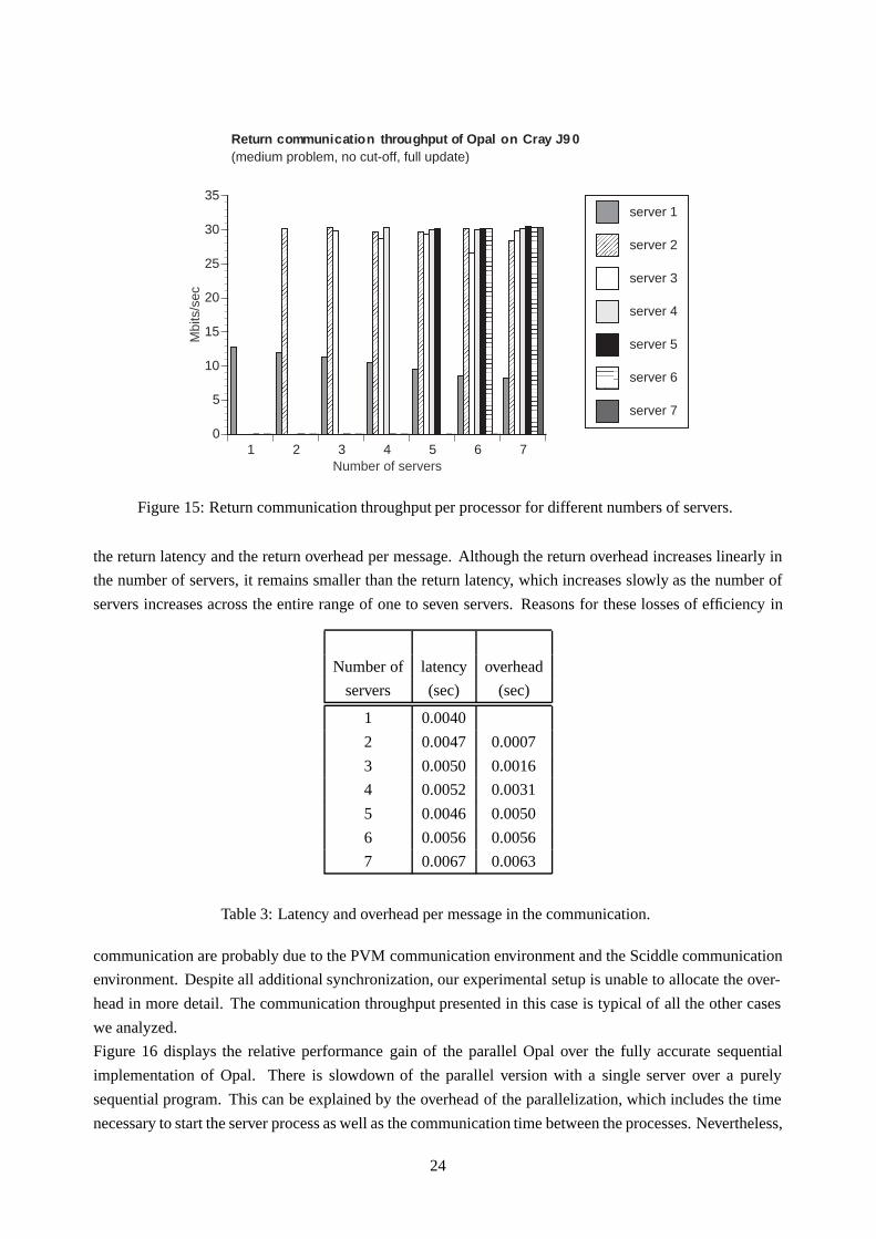
Figure 15: Return communication throughput per processor for different numbers of servers.
the return latency and the return overhead per message. Although the return overhead increases linearly in
the number of servers, it remains smaller than the return latency, which increases slowly as the number of
servers increases across the entire range of one to seven servers. Reasons for these losses of efficiency in
Number of latency overhead
servers (sec) (sec)
1 0.0040
2 0.0047 0.0007
3 0.0050 0.0016
4 0.0052 0.0031
5 0.0046 0.0050
6 0.0056 0.0056
7 0.0067 0.0063
Table 3: Latency and overhead per message in the communication.
communication are probably due to the PVM communication environment and the Sciddle communication
environment. Despite all additional synchronization, our experimental setup is unable to allocate the over-
head in more detail. The communication throughput presented in this case is typical of all the other cases
we analyzed.
Figure 16 displays the relative performance gain of the parallel Opal over the fully accurate sequential
implementation of Opal. There is slowdown of the parallel version with a single server over a purely
sequential program. This can be explained by the overhead of the parallelization, which includes the time
necessary to start the server process as well as the communication time between the processes. Nevertheless,
24

◆◆
◆◆
◆ ◆ ◆
1 2 3 4 5 6 70
1
2
3
4
5
6
7
Rel
ativ
e pe
rfor
man
ce g
ain
Number of servers
Performance gain(medium problem, no cut-off, full update)
Figure 16: The gain of parallel Opal over sequen-
tial Opal.
◆
◆
◆◆
◆◆
◆
1 2 3 4 5 6 70
1
2
3
4
5
6
7
Rel
ativ
e sp
eed-
up
Number of servers
Speed-up(medium problem, no cut-off, full update)
Figure 17: The speed-up of parallel Opal over
parallel Opal with one server.
this overhead is compensated by a parallel system of just two processors. Figure 17 shows the speed-up of
the parallel Opal over the parallel implementation with just one client and one server. The speedup becomes
significant with the increase of the number of servers: a high level of parallelism is achieved. We noted that
in both Figure 16 and Figure 17 the performance values have sudden drops when the number of servers is
even. This reduction is due to large idle time, which indicates a load balancing problem.
In the re-engineering process of Opal, for the parallelization we introduced new data structures, i.e., the lists
of mass center pairs on which the energy contributions of the non-bonded interactions are computed, and
new tasks, i.e. the update of these lists. The creation of these lists is only done once at the startup and their
maintenance, the update, is a repeated overhead encountered only in the parallel version of Opal code.
In the next experimental case we investigate what happens when we reduce the update frequency: with a
parameter value of 0�1 the update skips in 9 out of 10 simulation steps. The factor problem size and with it
the computation complexity keep their values.
5.2.2 Case 2: medium problem, no cut-off, partial update
In Case 2, we examine the performance of Opal simulating the same size molecular complex as in Case
1. Again, all the non-bonded interactions among the molecular complex atoms are considered. The update
parameter is set at 0.1 instead of 1: the update phase runs only one of every ten steps of the simulation (see
paragraph 3.1).
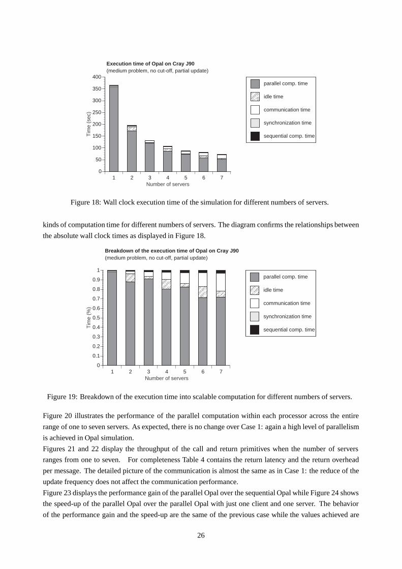
The wall clock execution time of the simulation, for different numbers of servers, is illustrated in Figure 18.
The chart shows that the parallel computation time is still the largest fraction of execution time: it decreases
almost linearly as the number of servers increases. Simultaneously, the communication time increases lin-
early, but its values remain much smaller than the parallel computation time. The synchronization time and
the sequential computation time remain insignificant compared to the overall execution time.
Similar to Case 1, a bad distribution of the work load, possible due to a load balancing problem, results
when the number of servers is even.
Figure 19 shows the breakdown of the communication time, the synchronization time, and the different
25
1 2 3 4 5 6 70
50
100
150
200
250
300
350
400
Tim
e (s
ec)
Number of servers
parallel comp. time
idle time
communication time
synchronization time
sequential comp. time
Execution time of Opal on Cray J90(medium problem, no cut-off, partial update)
Figure 18: Wall clock execution time of the simulation for different numbers of servers.
kinds of computation time for different numbers of servers. The diagram confirms the relationships between
the absolute wall clock times as displayed in Figure 18.
1 2 3 4 5 6 70
0.1
0.2
0.3
0.4
0.5
0.6
0.7
0.8
0.9
1
Tim
e (%
)
Number of servers
parallel comp. time
idle time
communication time
synchronization time
sequential comp. time
Breakdown of the execution time of Opal on Cray J90(medium problem, no cut-off, partial update)
Figure 19: Breakdown of the execution time into scalable computation for different numbers of servers.
Figure 20 illustrates the performance of the parallel computation within each processor across the entire
range of one to seven servers. As expected, there is no change over Case 1: again a high level of parallelism
is achieved in Opal simulation.
Figures 21 and 22 display the throughput of the call and return primitives when the number of servers
ranges from one to seven. For completeness Table 4 contains the return latency and the return overhead
per message. The detailed picture of the communication is almost the same as in Case 1: the reduce of the
update frequency does not affect the communication performance.
Figure 23 displays the performance gain of the parallel Opal over the sequential Opal while Figure 24 shows
the speed-up of the parallel Opal over the parallel Opal with just one client and one server. The behavior
of the performance gain and the speed-up are the same of the previous case while the values achieved are
26

1 2 3 4 5 6 70
10
20
30
40
50
60
70
80
90
MF
lOp/
sec
Number of servers
server 1
server 2
server 3
server 4
server 5
server 6
server 7
Local computation performance of Opal on Cray J90(medium problem, no cut-off, partial update)
Figure 20: Local computation performance per processor for different numbers of servers.
1 2 3 4 5 6 70
5
10
15
20
25
Mbi
ts/s
ec
Number of servers
server 1
server 2
server 3
server 4
server 5
server 6
server 7
Call communication throughput of Opal on Cray J90(medium problem, no cut-off, partial update)
Figure 21: Call communication throughput per processor for different numbers of servers.
27

1 2 3 4 5 6 70
5
10
15
20
25
30
35
Mbi
ts/s
ec
Number of servers
server 1
server 2
server 3
server 4
server 5
server 6
server 7
Return communication throughput of Opal on Cray J9 0(medium problem, no cut-off, partial update)
Figure 22: Return communication throughput per processor for different numbers of servers.
Number of latency overhead
servers (sec) (sec)
1 0.0038
2 0.0045 0.0007
3 0.0050 0.0016
4 0.0057 0.0025
5 0.0047 0.0045
6 0.0056 0.0055
7 0.0067 0.0063
Table 4: Latency and overhead per message in the communication.
28

◆◆
◆◆
◆ ◆◆
1 2 3 4 5 6 70
1
2
3
4
5
6
7
Rel
ativ
e pe
rfor
man
ce g
ain
Number of servers
Performance gain(medium problem, no cut-off, partial update)
Figure 23: The performance gain of parallel Opal
over sequential Opal.
◆
◆
◆◆
◆◆
◆
1 2 3 4 5 6 70
1
2
3
4
5
6
7
Rel
ativ
e sp
eed-
up
Number of servers
Speed-up(medium problem, no cut-off, partial update)
Figure 24: The speed-up of parallel Opal over
parallel Opal with one server.
larger.
In the next measurement case, the problem size is still the same and we investigate what happens when
we introduce an effective cut-off parameter (the cut-off parameter decreases from the non-effective value
of 60 A to the effective value of 10 A). The size of the lists becomes smaller than the Cases 1 and 2: a
large amount of the mass center pairs on which Opal computes the energy components of the non-bonded
interactions are cut. Also the update factor remains as in Case 1: the lists update is done at each step of the
simulation.
5.2.3 Case 3: medium problem, with cut-off, full update
In Case 3, we investigate the medium size problem but not all the non-bonded interactions among the
molecular complex atoms are considered: only the pairs of mass centers, whose distance is less than 10 A,
are examined. The computational complexity becomes linear in the number of atoms.
Figure 25 shows the wall clock execution time of the simulation for different numbers of servers. As the
number of servers increases, the communication time decreases linearly and becomes comparable with the
other time components. At the same time, the parallel computation time decreases, the synchronization time
increases slowly and the sequential computation time assumes constant values. All these different measured
execution times have now a varying impact on the overall execution time. Again, the chart shows a bad
distribution of the work load among the servers when the number of servers is even, but since the fraction
of computation time is lower, the idle times are less than in Case 1. The bad distribution causes some idle
time in some compute servers, that remains insignificant to the overall execution time.
Figure 26 displays the breakdown of the execution time, for different numbers of servers. The chart estab-
lishes the relationships between the absolute wall clock times as shown in Figure 25 and the occurrence of
an insignificant idle time when the number of servers is even.
Figure 27 presents the local computation performance per processor. Although the compute performance
per processor remains approximately constant like in the reference Case 1, the values achieved are smaller
in this case.
29

1 2 3 4 5 6 70
5
10
15
20
25
30
35
Tim
e (s
ec)
Number of servers
parallel comp. time
idle time
communication time
synchronization time
sequential comp. time
Execution time of Opal on Cray J90(medium problem, with cut-off, full update)
Figure 25: Wall clock execution time of the simulation for different numbers of servers.
1 2 3 4 5 6 70
0.1
0.2
0.3
0.4
0.5
0.6
0.7
0.8
0.9
1
Tim
e (%
)
Number of servers
parallel comp. time
idle time
communication time
synchronization time
sequential comp. time
Breakdown of the execution time of Opal on Cray J90(medium problem, with cut-off, full update)
Figure 26: Breakdown of the execution time into scalable computation for different numbers of servers.
30

1 2 3 4 5 6 70
10
20
30
40
50
60
70
80
90M
FlO
p/se
c
Number of servers
server 1
server 2
server 3
server 4
server 5
server 6
server 7
Local computation performance of Opal on Cray J90(medium problem, with cut-off, full update)
Figure 27: Local computation performance per processor for different numbers of servers.
The size of the call block to each server and the size of the return block from each server remain constant at
220 KBytes even though the computational complexity decreases from Case 1. The communication features
are almost the same as in the previous cases.
Figure 28 shows the gain of the parallel implementation over the sequential Opal. The different algorithm
with cut-off causes big performance gains over the original, sequential program without cut-off. The reduc-
tion of the computational effort causes a less accurate estimate of the energy. The gain decreases sharply
when the communication time becomes larger than the parallel computation time. Figure 29 illustrates the
speed-up of the parallel Opal versus the parallel implementation with just one client and one server. The
reduction of the amount of the parallel computation with the cut-off parameter limits the opportunity for
speed-up.
In the next measurement case, we investigate what happens when the order of the computation complexity
remains linear and we reduce the update frequency: the update is only done once every 10 simulation steps.
5.2.4 Case 4: medium problem, with cut-off, partial update
In Case 4,we investigate a last case with a medium size molecular complex this time including both effective
cut-off and partial update.
Figure 30 displays the wall clock execution time of the simulation for different numbers of servers. The chart
shows the amounts of communication time, parallel computation time as well as synchronization time. All
of them are 15� 30% smaller than in Case 3. As the number of servers increases, the parallel computation
time decreases linearly while the communication time increases. At the same time the synchronization time
increases slowly, while the sequential computation time remains constant. As in the previous case, all these
different execution times affect, each one in a different way, the overall execution time. A bad distribution of
the workload among the servers causes some idle time in some compute servers when the number of servers
is even but the amount of this idle time remains insignificant to the overall execution time like in Case 3.
31

◆
◆◆ ◆
◆◆
◆
1 2 3 4 5 6 70
2
4
6
8
10
12
Rel
ativ
e pe
rfor
man
ce g
ain
Number of servers
Performance gain(medium problem, with cutoff, full update)
Figure 28: The performance gain of parallel Opal
over sequential Opal.
◆◆ ◆ ◆ ◆ ◆ ◆
1 2 3 4 5 6 70
1
2
3
4
5
6
7
Rel
ativ
e sp
eed-
upNumber of servers
Speed-up(medium problem, with cut-off, full update)
Figure 29: The speed-up of parallel Opal over
parallel Opal with one server.
1 2 3 4 5 6 70
5
10
15
20
25
30
35
Tim
e (s
ec)
Number of servers
parallel comp. time
idle time
communication time
synchronization time
sequential comp. time
Execution time of Opal on Cray J90(medium problem, with cut-off, partial update)
Figure 30: Wall clock execution time of the simulation for different numbers of servers.
32

The breakdown of percentages for execution times is shown in Figure 31. The chart reiterates the relation-
ships between the absolute wall clock times as shown in Figure 30 and confirms the insignificance of the
idle time in this measurement.
1 2 3 4 5 6 70
0.1
0.2
0.3
0.4
0.5
0.6
0.7
0.8
0.9
1
Tim
e (%
)
Number of servers
parallel comp. time
idle time
communication time
synchronization time
sequential comp. time
Breakdown of the execution time of Opal on Cray J90(medium problem, with cut-off, partial update)
Figure 31: Breakdown of the execution time into scalable computation for different numbers of servers.
Figure 32 illustrates the performance of the parallel computation per processor for different numbers of
servers. The reduced update leads to a slight further decrease of the local computation performance com-
pared with the previous case. While in the previous case the performance values were the average of both
the update routine and the energy computation routine, in this case the performance values are evaluated on
the single energy computation routine.
1 2 3 4 5 6 70
10
20
30
40
50
60
70
80
90
MF
lOp/
sec
number of servers
server 1
server 2
server 3
server 4
server 5
server 6
server 7
Local computation performance of Opal on Cray J90(medium problem, with cut-off, partial update)
Figure 32: Local computation performance per processor for different numbers of servers.
The picture of the communication efficiency remains unchanged.
33

Figure 33 shows the performance gain of the parallel Opal over the sequential Opal while Figure 34 shows
the speed-up of the parallel Opal over the parallel Opal with one client and one server. The reduced update
frequency leads to smaller parallel computation time and higher values of gain than in the previous case. As
in Case 3, the gain decreases as the communication time becomes larger than the parallel computation time.
The speed-up is almost the same of the previous case.
◆
◆◆ ◆
◆◆
◆
1 2 3 4 5 6 70
2
4
6
8
10
12
14
16
Rel
ativ
e pe
rfor
man
ce g
ain
Number of servers
Performance gain(medium problem, with cut-off, patial update)
Figure 33: The gain of parallel Opal over sequen-
tial Opal.
◆◆ ◆ ◆ ◆ ◆ ◆
a 1 2 3 4 5 6 70
1
2
3
4
5
6
7
Rel
ativ
e sp
eed-
up
Number of servers
Speed-up(medium problem, with cut-off, patial update)
Figure 34: The speed-up of parallel Opal over
parallel Opal with one server.
In the next measurement Cases, 5, 6, 7, and 8, we investigate the impact of a different problem size on the
different measured execution times: the size of the problem becomes larger.
5.2.5 Case 5: large problem, no cut-off, full update
In Case 5, we investigate the performance of Opal simulating a large size molecular complex, the NMR
structure of the LFB homeodomain immersed in 4634 water molecules. All the non-bonded interactions
among the atoms are considered and the update of the lists is done at each step of the simulation.
Figure 35 illustrates the execution time (wall clock) of the simulation for different numbers of servers. The
chart shows that the largest fraction of execution time, the time in parallel computation, decreases linearly as
the number of servers increases. At the same time the communication time increases linearly but its overall
size remains smaller than the parallel computation time across the entire range of one to seven servers. The
synchronization time and the sequential computation time remain insignificant to the overall execution time.
When the number of servers is even, there is idle time in some compute servers (load balancing problem).
Figure 36 shows the breakdown of the execution time, communication time, synchronization time, and
different kinds of computation time, for different numbers of servers. The chart illustrates the occurrence
of a significant idle time when the number of servers is even and confirms the relationships between the
absolute wall clock times as shown in Figure 35.
A larger problem size causes larger execution times than in Cases 1-4. At the same time we note that the
behavior of the time components is very similar to Case 1.
Figure 37 shows the performance of the parallel computation within each processor for the different numbers
of servers. The Opal simulation with this parameter set achieves high levels of parallelism as in Case 1.
34
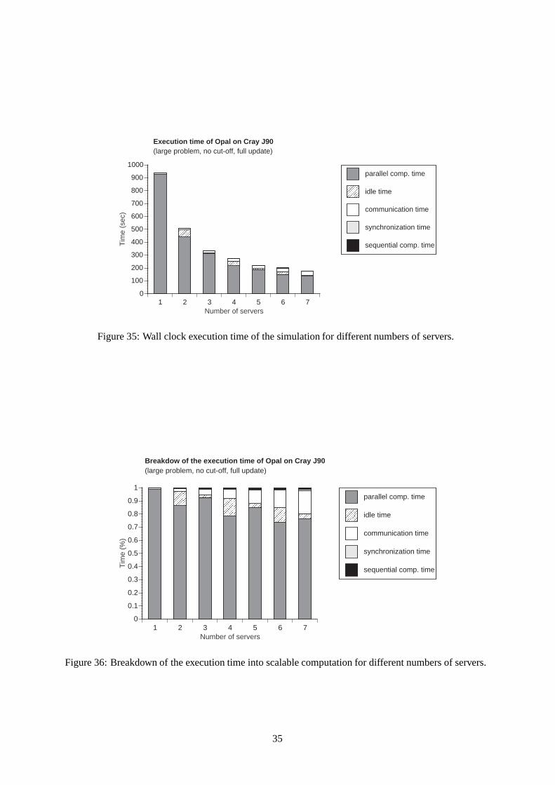
1 2 3 4 5 6 70
100
200
300
400
500
600
700
800
900
1000
Tim
e (s
ec)
Number of servers
parallel comp. time
idle time
communication time
synchronization time
sequential comp. time
Execution time of Opal on Cray J90(large problem, no cut-off, full update)
Figure 35: Wall clock execution time of the simulation for different numbers of servers.
1 2 3 4 5 6 70
0.1
0.2
0.3
0.4
0.5
0.6
0.7
0.8
0.9
1
Tim
e (%
)
Number of servers
parallel comp. time
idle time
communication time
synchronization time
sequential comp. time
Breakdow of the execution time of Opal on Cray J90(large problem, no cut-off, full update)
Figure 36: Breakdown of the execution time into scalable computation for different numbers of servers.
35

1 2 3 4 5 6 70
10
20
30
40
50
60
70
80
90M
FlO
p/se
c
Number of servers
server 1
server 2
server 3
server 4
server 5
server 6
server 7
Local computation performance of Opal on Cray J90(large problem, no cut-off, full update)
Figure 37: Local computation performance per processor for different numbers of servers.
Figure 38 and Figure 39 show communication throughput for call and return phases for different numbers
of servers and Table 5 shows the return latency and the return overhead per message. Although the size of
1 2 3 4 5 6 70
5
10
15
20
25
Mbi
ts/s
ec
Number of servers
server 1
server 2
server 3
server 4
server 5
server 6
server 7
Call communication throughput of Opal on Cray J90(large problem, no cut-off, full update)
Figure 38: Call communication throughput per processor for different numbers of servers.
the problem increases, the communication features are almost the same as in the previous cases.
Figure 40 shows the performance gain of parallel Opal over sequential Opal while Figure 41 displays the
speed-up of the parallel Opal over the parallel Opal with just one client and one server. In this case, the
higher values of parallel gain and speed-up are achieved due to the large amount of parallel computation in
the large size problem.
In the next measurement case, we investigate the impact of the reduction of the updates on the different
36
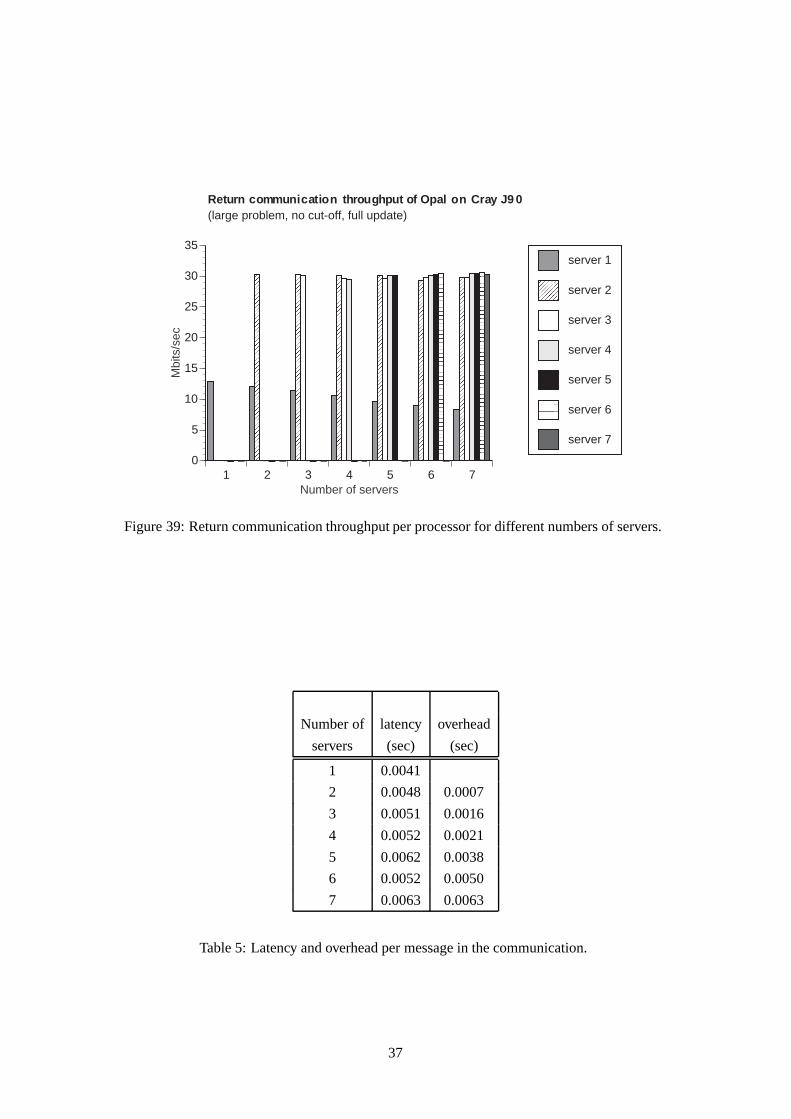
1 2 3 4 5 6 70
5
10
15
20
25
30
35
Mbi
ts/s
ec
Number of servers
server 1
server 2
server 3
server 4
server 5
server 6
server 7
Return communication throughput of Opal on Cray J9 0(large problem, no cut-off, full update)
Figure 39: Return communication throughput per processor for different numbers of servers.
Number of latency overhead
servers (sec) (sec)
1 0.0041
2 0.0048 0.0007
3 0.0051 0.0016
4 0.0052 0.0021
5 0.0062 0.0038
6 0.0052 0.0050
7 0.0063 0.0063
Table 5: Latency and overhead per message in the communication.
37

◆◆
◆◆
◆ ◆◆
1 2 3 4 5 6 70
1
2
3
4
5
6
7
Rel
ativ
e pe
rfor
man
ce g
ain
Number of servers
Performance gain(large problem, no cut-off, full update)
Figure 40: The performance gain of parallel Opal
over sequential Opal.
◆
◆
◆◆
◆◆
◆
1 2 3 4 5 6 70
1
2
3
4
5
6
7
Rel
ativ
e sp
eed-
up
Number of servers
Speed-up(large problem, no cut-off, full update)
Figure 41: The speed-up of parallel Opal over
parallel Opal with one server.
measured execution times while the problem size and the algorithm (no cut-off) remain the same.
5.2.6 Case 6: large problem, no cut-off, partial update
In Case 6, we investigate the performance of Opal simulating a large size molecular complex as in the
previous case. Like in Case 5, all the non-bonded interactions are considered; only the update parameter
decreases from 1 to 0.1 and the update phase runs each ten steps of the simulation.
Figure 42 shows the wall clock execution time of the simulation for different numbers of servers. The
features of the time components remain the same as in the previous case.
Again, when the number of servers is even, there is a bad distribution of the work load among the servers
which causes some idle time in some compute servers.
1 2 3 4 5 6 70
100
200
300
400
500
600
700
800
900
1000
Tim
e (s
ec)
Number of servers
parallel comp. time
idle time
communication time
synchronization time
sequential comp. time
Execution time of Opal on Cray J90(large problem, no cut-off, full update)
Figure 42: Wall clock execution time of the simulation for different numbers of servers.
Figure 43 shows the breakdown of the execution time into scalable computation for different number of
servers.
38

1 2 3 4 5 6 70
0.1
0.2
0.3
0.4
0.5
0.6
0.7
0.8
0.9
1T
ime
(%)
Number of servers
parallel comp. time
idle time
communication time
synchronization time
sequential comp. time
Breakdown of the execution time of Opal on Cray J90(large problem, no cut-off, partial update)
Figure 43: Breakdown of the execution time into scalable computation for different numbers of servers.
Figure 44 shows the performance of the parallel computation within each processor for the different numbers
of servers. The simulation achieves the same level of parallelism already achieved in Cases 1-2, and 5.
1 2 3 4 5 6 70
10
20
30
40
50
60
70
80
90
MF
lOp/
sec
Number of servers
server 1
server 2
server 3
server 4
server 5
server 6
server 7
Local computation performance of Opal on Cray J90(large problem, no cut-off, partial update)
Figure 44: Local computation performance per processor for different numbers of servers.
The communication remains unchanged as in the previous case.
Figure 46 displays the performance gain of the parallel Opal, with respect to the sequential Opal while
Figure 46 shows the speed-up of the parallel Opal over the parallel Opal with just one client and one server.
The gain as well as the speed-ups have the same behavior of Case 5 but their values are larger.
In the next measurement case we investigate what happens when we reduce the cut-off parameter from an
non-effective value of 60 A to an effective value of 10 A.
A large amount of the pairs of mass centers are cut from the lists which size becomes smaller than in Cases
5 and 6. The problem size factor keeps its value while the update of the lists is done at each step of the
39
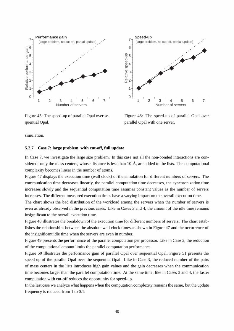
◆◆
◆◆
◆ ◆◆
1 2 3 4 5 6 70
1
2
3
4
5
6
7
Rel
ativ
e pe
rfor
man
ce g
ain
Number of servers
Performance gain(large problem, no cut-off, partial update)
Figure 45: The speed-up of parallel Opal over se-
quential Opal.
◆
◆
◆◆
◆◆
◆
1 2 3 4 5 6 70
1
2
3
4
5
6
7
Rel
ativ
e sp
eed-
up
Number of servers
Speed-up(large problem, no cut-off, partial update)
Figure 46: The speed-up of parallel Opal over
parallel Opal with one server.
simulation.
5.2.7 Case 7: large problem, with cut-off, full update
In Case 7, we investigate the large size problem. In this case not all the non-bonded interactions are con-
sidered: only the mass centers, whose distance is less than 10 A, are added to the lists. The computational
complexity becomes linear in the number of atoms.
Figure 47 displays the execution time (wall clock) of the simulation for different numbers of servers. The
communication time decreases linearly, the parallel computation time decreases, the synchronization time
increases slowly and the sequential computation time assumes constant values as the number of servers
increases. The different measured execution times have a varying impact on the overall execution time.
The chart shows the bad distribution of the workload among the servers when the number of servers is
even as already observed in the previous cases. Like in Cases 3 and 4, the amount of the idle time remains
insignificant to the overall execution time.
Figure 48 illustrates the breakdown of the execution time for different numbers of servers. The chart estab-
lishes the relationships between the absolute wall clock times as shown in Figure 47 and the occurrence of
the insignificant idle time when the servers are even in number.
Figure 49 presents the performance of the parallel computation per processor. Like in Case 3, the reduction
of the computational amount limits the parallel computation performance.
Figure 50 illustrates the performance gain of parallel Opal over sequential Opal, Figure 51 presents the
speed-up of the parallel Opal over the sequential Opal. Like in Case 3, the reduced number of the pairs
of mass centers in the lists introduces high gain values and the gain decreases when the communication
time becomes larger than the parallel computation time. At the same time, like in Cases 3 and 4, the faster
computation with cut-off reduces the opportunity for speed-up.
In the last case we analyze what happens when the computation complexity remains the same, but the update
frequency is reduced from 1 to 0.1.
40

1 2 3 4 5 6 70
10
20
30
40
50
60
Tim
e (s
ec)
Number of servers
parallel comp. time
idle time
communication time
synchronization time
sequential comp. time
Execution time of Opal on Cray J90(large problem, with cut-off, full update)
Figure 47: Wall clock execution time of the simulation for different numbers of servers.
1 2 3 4 5 6 70
0.1
0.2
0.3
0.4
0.5
0.6
0.7
0.8
0.9
1
Tim
e (%
)
Number of servers
parallel comp. time
idle time
communication time
synchronization time
sequential comp. time
Breakdown of the execution time of Opal on Cray J90(large problem, with cut-off, full update)
Figure 48: Breakdown of the execution time into scalable computation for different numbers of servers.
41

1 2 3 4 5 6 70
10
20
30
40
50
60
70
80
90
MF
lOp/
sec
Number of servers
server 1
server 2
server 3
server 4
server 5
server 6
server 7
Local computation performance of Opal on Cray J90(large problem, with cut-off, full update)
Figure 49: Local computation performance per processor for different numbers of servers.
◆
◆◆ ◆
◆◆
◆
1 2 3 4 5 6 70
2
4
6
8
10
12
14
16
Rel
ativ
e pe
rfor
man
ce g
ain
Number of servers
Performance gain(large problem, with cut-off, full update)
Figure 50: The performance gain of parallel Opal
over sequential Opal.
◆◆ ◆ ◆ ◆ ◆ ◆
1 2 3 4 5 6 70
1
2
3
4
5
6
7
Rel
ativ
e sp
eed-
up
Number of servers
Speed-up(large problem, with cut-off, full update)
Figure 51: The speed-up of parallel Opal over
parallel Opal with one server.
42
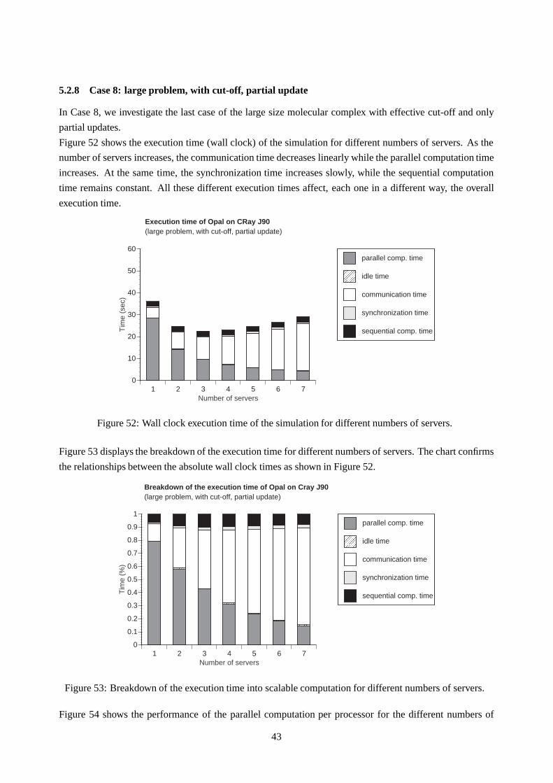
5.2.8 Case 8: large problem, with cut-off, partial update
In Case 8, we investigate the last case of the large size molecular complex with effective cut-off and only
partial updates.
Figure 52 shows the execution time (wall clock) of the simulation for different numbers of servers. As the
number of servers increases, the communication time decreases linearly while the parallel computation time
increases. At the same time, the synchronization time increases slowly, while the sequential computation
time remains constant. All these different execution times affect, each one in a different way, the overall
execution time.
1 2 3 4 5 6 70
10
20
30
40
50
60
Tim
e (s
ec)
Number of servers
parallel comp. time
idle time
communication time
synchronization time
sequential comp. time
Execution time of Opal on CRay J90(large problem, with cut-off, partial update)
Figure 52: Wall clock execution time of the simulation for different numbers of servers.
Figure 53 displays the breakdown of the execution time for different numbers of servers. The chart confirms
the relationships between the absolute wall clock times as shown in Figure 52.
1 2 3 4 5 6 70
0.1
0.2
0.3
0.4
0.5
0.6
0.7
0.8
0.9
1
Tim
e (%
)
Number of servers
parallel comp. time
idle time
communication time
synchronization time
sequential comp. time
Breakdown of the execution time of Opal on Cray J90(large problem, with cut-off, partial update)
Figure 53: Breakdown of the execution time into scalable computation for different numbers of servers.
Figure 54 shows the performance of the parallel computation per processor for the different numbers of
43
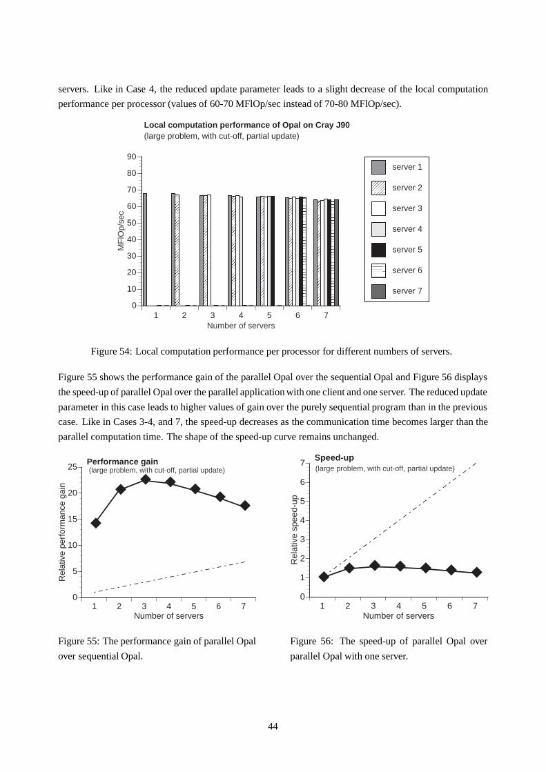
servers. Like in Case 4, the reduced update parameter leads to a slight decrease of the local computation
performance per processor (values of 60-70 MFlOp/sec instead of 70-80 MFlOp/sec).
1 2 3 4 5 6 70
10
20
30
40
50
60
70
80
90
MF
lOp/
sec
Number of servers
server 1
server 2
server 3
server 4
server 5
server 6
server 7
Local computation performance of Opal on Cray J90(large problem, with cut-off, partial update)
Figure 54: Local computation performance per processor for different numbers of servers.
Figure 55 shows the performance gain of the parallel Opal over the sequential Opal and Figure 56 displays
the speed-up of parallel Opal over the parallel application with one client and one server. The reduced update
parameter in this case leads to higher values of gain over the purely sequential program than in the previous
case. Like in Cases 3-4, and 7, the speed-up decreases as the communication time becomes larger than the
parallel computation time. The shape of the speed-up curve remains unchanged.
◆
◆◆ ◆
◆◆
◆
1 2 3 4 5 6 70
5
10
15
20
25
Rel
ativ
e pe
rfor
man
ce g
ain
Number of servers
Performance gain(large problem, with cut-off, partial update)
Figure 55: The performance gain of parallel Opal
over sequential Opal.
◆◆ ◆ ◆ ◆ ◆ ◆
1 2 3 4 5 6 70
1
2
3
4
5
6
7
Rel
ativ
e sp
eed-
up
Number of servers
Speed-up(large problem, with cut-off, partial update)
Figure 56: The speed-up of parallel Opal over
parallel Opal with one server.
44
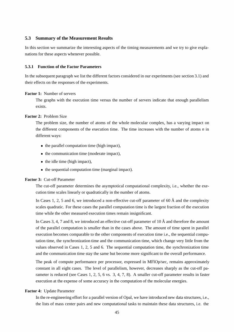
5.3 Summary of the Measurement Results
In this section we summarize the interesting aspects of the timing measurements and we try to give expla-
nations for these aspects whenever possible.
5.3.1 Function of the Factor Parameters
In the subsequent paragraph we list the different factors considered in our experiments (see section 3.1) and
their effects on the responses of the experiments.
Factor 1: Number of servers
The graphs with the execution time versus the number of servers indicate that enough parallelism
exists.
Factor 2: Problem Size
The problem size, the number of atoms of the whole molecular complex, has a varying impact on
the different components of the execution time. The time increases with the number of atoms n in
different ways:
� the parallel computation time (high impact),
� the communication time (moderate impact),
� the idle time (high impact),
� the sequential computation time (marginal impact).
Factor 3: Cut-off Parameter
The cut-off parameter determines the asymptotical computational complexity, i.e., whether the exe-
cution time scales linearly or quadratically in the number of atoms.
In Cases 1, 2, 5 and 6, we introduced a non-effective cut-off parameter of 60 A and the complexity
scales quadratic. For these cases the parallel computation time is the largest fraction of the execution
time while the other measured execution times remain insignificant.
In Cases 3, 4, 7 and 8, we introduced an effective cut-off parameter of 10 A and therefore the amount
of the parallel computation is smaller than in the cases above. The amount of time spent in parallel
execution becomes comparable to the other components of execution time i.e., the sequential compu-
tation time, the synchronization time and the communication time, which change very little from the
values observed in Cases 1, 2, 5 and 6. The sequential computation time, the synchronization time
and the communication time stay the same but become more significant to the overall performance.
The peak of compute performance per processor, expressed in MFlOp/sec, remains approximately
constant in all eight cases. The level of parallelism, however, decreases sharply as the cut-off pa-
rameter is reduced (see Cases 1, 2, 5, 6 vs. 3, 4, 7, 8). A smaller cut-off parameter results in faster
execution at the expense of some accuracy in the computation of the molecular energies.
Factor 4: Update Parameter
In the re-engineering effort for a parallel version of Opal, we have introduced new data structures, i.e.,
the lists of mass center pairs and new computational tasks to maintain these data structures, i.e. the
45
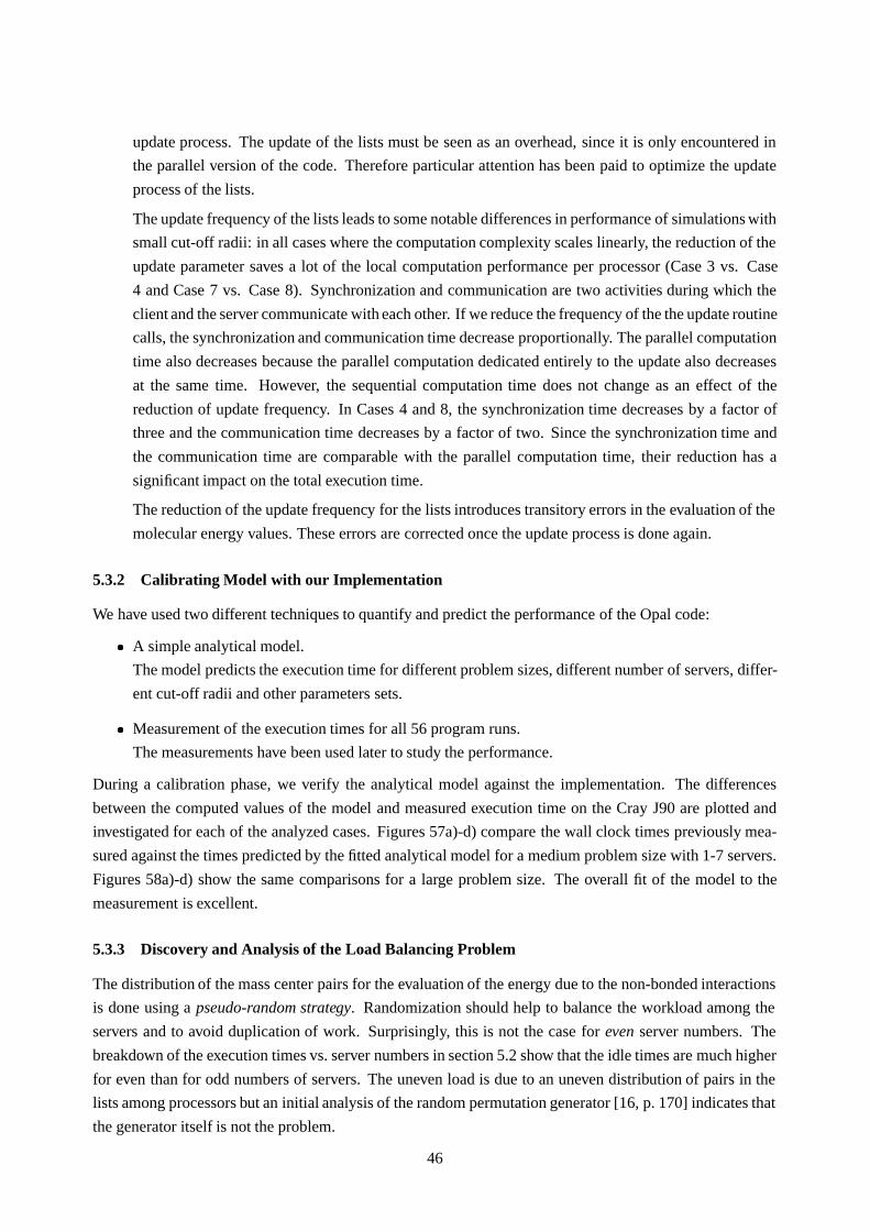
update process. The update of the lists must be seen as an overhead, since it is only encountered in
the parallel version of the code. Therefore particular attention has been paid to optimize the update
process of the lists.
The update frequency of the lists leads to some notable differences in performance of simulations with
small cut-off radii: in all cases where the computation complexity scales linearly, the reduction of the
update parameter saves a lot of the local computation performance per processor (Case 3 vs. Case
4 and Case 7 vs. Case 8). Synchronization and communication are two activities during which the
client and the server communicate with each other. If we reduce the frequency of the the update routine
calls, the synchronization and communication time decrease proportionally. The parallel computation
time also decreases because the parallel computation dedicated entirely to the update also decreases
at the same time. However, the sequential computation time does not change as an effect of the
reduction of update frequency. In Cases 4 and 8, the synchronization time decreases by a factor of
three and the communication time decreases by a factor of two. Since the synchronization time and
the communication time are comparable with the parallel computation time, their reduction has a
significant impact on the total execution time.
The reduction of the update frequency for the lists introduces transitory errors in the evaluation of the
molecular energy values. These errors are corrected once the update process is done again.
5.3.2 Calibrating Model with our Implementation
We have used two different techniques to quantify and predict the performance of the Opal code:
� A simple analytical model.
The model predicts the execution time for different problem sizes, different number of servers, differ-
ent cut-off radii and other parameters sets.
� Measurement of the execution times for all 56 program runs.
The measurements have been used later to study the performance.
During a calibration phase, we verify the analytical model against the implementation. The differences
between the computed values of the model and measured execution time on the Cray J90 are plotted and
investigated for each of the analyzed cases. Figures 57a)-d) compare the wall clock times previously mea-
sured against the times predicted by the fitted analytical model for a medium problem size with 1-7 servers.
Figures 58a)-d) show the same comparisons for a large problem size. The overall fit of the model to the
measurement is excellent.
5.3.3 Discovery and Analysis of the Load Balancing Problem
The distribution of the mass center pairs for the evaluation of the energy due to the non-bonded interactions
is done using a pseudo-random strategy. Randomization should help to balance the workload among the
servers and to avoid duplication of work. Surprisingly, this is not the case for even server numbers. The
breakdown of the execution times vs. server numbers in section 5.2 show that the idle times are much higher
for even than for odd numbers of servers. The uneven load is due to an uneven distribution of pairs in the
lists among processors but an initial analysis of the random permutation generator [16, p. 170] indicates that
the generator itself is not the problem.
46
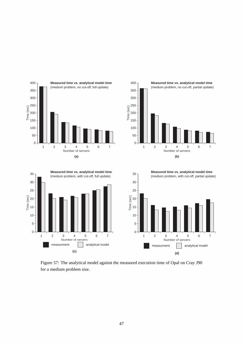
1 2 3 4 5 6 70
50
100
150
200
250
300
350
400
Tim
e (s
ec)
Number of servers1 2 3 4 5 6 7
0
50
100
150
200
250
300
350
400
Tim
e (s
ec)
Number of servers
1 2 3 4 5 6 70
5
10
15
20
25
30
35
Tim
e (s
ec)
Number of servers
measurment analytical model
1 2 3 4 5 6 70
5
10
15
20
25
30
35
Tim
e (s
ec)
Number of servers
measurment analytical model
Measured time vs. analytical model time(medium problem, no cut-off, full update)
Measured time vs. analytical model time(medium problem, no cut-off, partial update)
Measured time vs. analytical model time(medium problem, with cut-off, full update)
Measured time vs. analytical model time(medium problem, with cut-off, partial update)
(a) (b)
(c)(d)
Figure 57: The analytical model against the measured execution time of Opal on Cray J90
for a medium problem size.
47

1 2 3 4 5 6 70
100
200
300
400
500
600
700
800
900
1000
Tim
e (s
ec)
Number of servers
Measured time vs. analytical model time(large problem, no cut-off, full update)
1 2 3 4 5 6 70
100
200
300
400
500
600
700
800
900
1000
Tim
e (s
ec)
Number of servers
Measured time vs. analytical model time:(large problem, no cut-off, partial update)
1 2 3 4 5 6 70
10
20
30
40
50
60
Tim
e (s
ec)
Number of servers
measurement analytical model
Measured time vs. analytical model time:(large problem, with cut-off, full update)
1 2 3 4 5 6 70
10
20
30
40
50
60
Tim
e (s
ec)
Number of servers
measurement analytical model
Measured time vs. analytical model time:(large problem, with cut-off, partial update)
(a) (b)
(d)(c)
Figure 58: The analytical model against the measured execution time of Opal on Cray J90
for a large problem size.
48
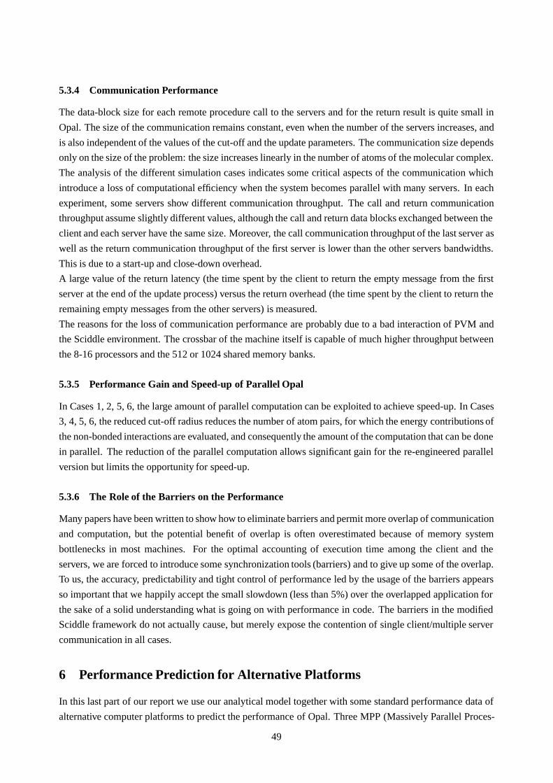
5.3.4 Communication Performance
The data-block size for each remote procedure call to the servers and for the return result is quite small in
Opal. The size of the communication remains constant, even when the number of the servers increases, and
is also independent of the values of the cut-off and the update parameters. The communication size depends
only on the size of the problem: the size increases linearly in the number of atoms of the molecular complex.
The analysis of the different simulation cases indicates some critical aspects of the communication which
introduce a loss of computational efficiency when the system becomes parallel with many servers. In each
experiment, some servers show different communication throughput. The call and return communication
throughput assume slightly different values, although the call and return data blocks exchanged between the
client and each server have the same size. Moreover, the call communication throughput of the last server as
well as the return communication throughput of the first server is lower than the other servers bandwidths.
This is due to a start-up and close-down overhead.
A large value of the return latency (the time spent by the client to return the empty message from the first
server at the end of the update process) versus the return overhead (the time spent by the client to return the
remaining empty messages from the other servers) is measured.
The reasons for the loss of communication performance are probably due to a bad interaction of PVM and
the Sciddle environment. The crossbar of the machine itself is capable of much higher throughput between
the 8-16 processors and the 512 or 1024 shared memory banks.
5.3.5 Performance Gain and Speed-up of Parallel Opal
In Cases 1, 2, 5, 6, the large amount of parallel computation can be exploited to achieve speed-up. In Cases
3, 4, 5, 6, the reduced cut-off radius reduces the number of atom pairs, for which the energy contributions of
the non-bonded interactions are evaluated, and consequently the amount of the computation that can be done
in parallel. The reduction of the parallel computation allows significant gain for the re-engineered parallel
version but limits the opportunity for speed-up.
5.3.6 The Role of the Barriers on the Performance
Many papers have been written to show how to eliminate barriers and permit more overlap of communication
and computation, but the potential benefit of overlap is often overestimated because of memory system
bottlenecks in most machines. For the optimal accounting of execution time among the client and the
servers, we are forced to introduce some synchronization tools (barriers) and to give up some of the overlap.
To us, the accuracy, predictability and tight control of performance led by the usage of the barriers appears
so important that we happily accept the small slowdown (less than 5%) over the overlapped application for
the sake of a solid understanding what is going on with performance in code. The barriers in the modified
Sciddle framework do not actually cause, but merely expose the contention of single client/multiple server
communication in all cases.
6 Performance Prediction for Alternative Platforms
In this last part of our report we use our analytical model together with some standard performance data of
alternative computer platforms to predict the performance of Opal. Three MPP (Massively Parallel Proces-
49

sor) platforms are considered for our “what would be the performance, if Opal ran there...” study in addition
to the Cray J90: a Cray T3E “big iron” and three flavors of PC Clusters: slow CoPs (Cluster of PCs), SMP
CoPs and fast CoPs. We call the first PCs Cluster slow since it is optimized for lowest cost; connected with
shared 100BaseT Ethernet its processors are just single 200MHz Intel Pentium Pro. The SMP CoPs plat-
form is based on some twin 200MHz Intel Pentium Pro processors and SCI shared memory interconnects,
while the fast PCs Cluster has single 400MHz Intel Pentium Pro processor per node and features fast com-
munication with fully switched Gigabit/s Myrinet Interconnects. Comparable Clusters of PCs installations
are described in [4, 6, 20].
6.1 Extraction of Model Parameters for Alternatives
The parameters of our analytical model were intentionally chosen to include all major technical data usually
published for parallel machines. This includes among others: message overhead, message throughput,
computation rate for SAXPY inner loops and time to synchronize all participating processors. For each new
platform we determine the key parameters by the execution of a few micro-benchmarks, verified against
published performance figures [12]. An overview of the data used is found in Tables 6 and 7.
MPP Execution Floating Point Computation Relative Adjusted
Node Time op. counted Rate Time Computation Rate
Type on single node on single node on single node on single no de
(clock speed) [s] [MFlOp] [MFlOp/s] [%] [MFlOp/s]
Cray T3E-900 9.56 811.71 85 138 52
(450 MHz)
Cray J90 Classic 6.18 497.55 80 a 100 80
(100 MHz)
Slow CoPs 10.00 327.40 32 65 50
(200 MHz)
SMP CoPs 5.00 327.40 65 65 100
(2*200 MHz)
Fast CoPs 4.85 325.80 67 65 102
(400 MHz)
Table 6: Computation speed parameters used for performance prediction of Opal on all four
different platforms. The numbers reflect the performance of the isolated Opal application
kernel used as a microbenchmark.aFor fall 98 our J90 Classics are scheduled for an upgrade to the new v vector processors that significantly
enhance the computational throughput
We use these figures together with the formulas of the analytical model to predict the execution time of Opal
with a large size molecular complex in varying configurations. Some model parameters are intrinsic to Opal
itself and invariant across the different machines. Those parameters are simply kept at their level measured
with the J90. On the other hand, we have had to select the most important platform parameters,which depend
on the new machines features. The observed MBytes/s in Table 7 are relevant to the model parameters a1
50

MPP MByte/s MByte/s Latency
Node on single node on single node on single node
Type (hw peak) (observed) (observed)
Cray T3E-900 (MPI) 350 100 12 µsec
Cray J90 (PVM/Sciddle) 2000/8 3 10 msec
Slow CoPs (Ethernet) 10 3 10 msec
SMP CoPs 50 15 25 µsec
Fast CoPs (Myrinet) 125 30 15 µsec
Table 7: Communication speed parameters used for performance prediction of Opal for all
four different platforms. The numbers are obtained from microbenchmarks and verified
against published values
and b1. The model parameters a2 and a3 are indirectly achieved using the data in Table 6 and computing the
average time used to generate a pair of atoms and calculate the distance between them as well as to compute
the non-bonded energy contribution of a single pair of atoms.
Since the model captures the parallelization and adjusts to different processor performance, we can calculate
the estimated execution time and the relative speed-up achieved on each new platform and compare it with
the measured speed-up achieved on a Cray J90.
As for many scientific codes, one routine of Opal dominates the compute performance. This routine was
benchmarked on each platform using the most accurate cycle counters and floating point performance mon-
itoring hardware that is actually present on all four machine types. The most important surprise was a sig-
nificant difference in floating point operations for the different platform although the arithmetic was 64bit
in all cases and the results were precisely identical (or within the floating point epsilon for comparisons be-
tween Cray and IEEE arithmetic). The differences are due to the different compilers or intrinsics functions.
We eliminate this difference by assuming that the best compiler (i.e. the PGI compiler for the PCs [14]) is
setting a lower bound for the computation and adjust the local compute rate (MFlop/s) of other platforms
accordingly.
The communication performance is even more difficult to compare in real applications. Some bad inter-
actions between middleware and PVM library reduces the measured communication rate on the Cray J90
processor to about 3 MByte/s, despite its more than one GByte/s strong crossbar interconnect between the 8
processor boards and the memory banks. The authors of the Sciddle middleware claim that they measured
up to 7 MByte/s for a synthetic Sciddle RPC example and that this matches the performance of PVM 3.0
on the machine [2]. It certainly remains below to what this machine is capable of in shared memory mode.
At the same time we assume that with the right configuration of PVM flags or at least with a rewrite of the
middleware to use PVM in true zero copy mode, we could significantly improve the performance of Opal
on the J90, but such work is outside the scope of our performance study.
For the other platforms we assumed an MPI or PVM based implementation without Sciddle and deduced
our performance numbers mainly from MPI micro-benchmarks gathered by our students and from similar
numbers published by independent researchers on the internet (e.g. [12]).
51
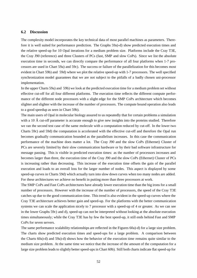
6.2 Discussion
The complexity model incorporates the key technical data of most parallel machines as parameters. There-
fore it is well suited for performance prediction. The Graphs 59a)-d) show predicted execution times and
the relative speed-up for 10 Opal iterations for a medium problem size. Platforms include the Cray T3E,
the Cray J90 (reference) and three Clusters of PCs (fast, SMP and slow CoPs). Since we list the absolute
execution time in seconds, we can directly compare the performance of all four platforms when 1-7 pro-
cessors are used in Chart 59a) and 59c). The success or failure of the parallelization for this becomes most
evident in Chart 59b) and 59d) where we plot the relative speed-up with 1-7 processors. The well specified
synchronization model guarantees that we are not subject to the pitfalls of a badly chosen uni-processor
implementation.
In the upper Charts 59a) and 59b) we look at the predicted execution time for a medium problem set without
effective cut-off for all four different platforms. The execution time reflects the different compute perfor-
mance of the different node processors with a slight edge for the SMP CoPs architecture which becomes
slighter and slighter with the increase of the number of processors. The compute bound operation also leads
to a good speedup as seen in Chart 59b).
The main users of Opal in molecular biology assured to us repeatedly that for certain problems a simulation
with a 10 A cut-off parameter is accurate enough to give new insights into the proteins studied. Therefore
we ran the second test case of the same molecule with a computation reduced by cut-off. In the lower two
Charts 59c) and 59d) the computation is accelerated with the effective cut-off and therefore the Opal run
becomes gradually communication bounded as the parallelism increases. In this case the communication
performance of the machine does matter a lot. The Cray J90 and the slow CoPs (Ethernet) Cluster of
PCs are severely limited by their slow communication hardware or by their bad software infrastructure for
message passing. This is visible in predicted execution times: as the number of processors increases and
becomes larger than three, the execution time of the Cray J90 and the slow CoPs (Ethernet) Cluster of PCs
is increasing rather than decreasing. This increase of the execution time offsets the gain of the parallel
execution and loads to an overall loss for the larger number of nodes. This aspect is displayed by some
speed-up curves in Charts 59d) which actually turn into slow down curves when too many nodes are added.
For these architectures we achieve no benefit in putting more than three processors at work.
The SMP CoPs and Fast CoPs architectures have already lower execution time than the big irons for a small
number of processors. However with the increase of the number of processors, the speed of the Cray T3E
catches up due to the good communication time. This trend is also evident in the speed-up curves where the
Cray T3E architecture achieves better gain and speed-up. For the platforms with the better communication
systems we can scale the application nicely to 7 processor with a speed-up of 4 or greater. As we can see
in the lower Graphs 59c) and d), speed-up can not be interpreted without looking at the absolute execution
times simultaneously; while the Cray T3E has by few the best speed-up, it still ends behind Fast and SMP
CoPs for seven servers.
The same performance scalability relationships are reflected in the Figures 60a)-d) for a large size problem.
The charts show predicted execution times and speed-ups for a large problem. A comparison between
the Charts 60a)-d) and 59a)-d) shows how the behavior of the execution time remains quite similar to the
medium size problem. At the same time we notice that the increase of the amount of the computation for a
large size problem leads to slightly better speed-ups in Chart 60b). Still both charts indicate flat speed-up for
52
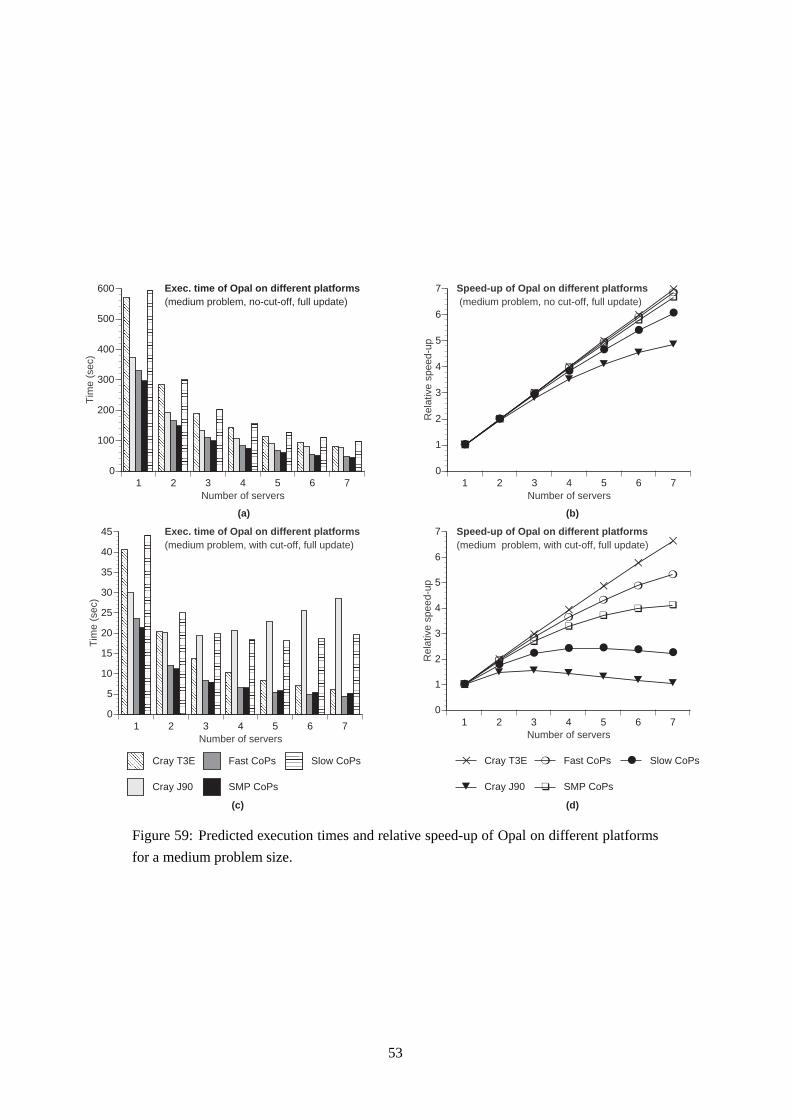
1 2 3 4 5 6 70
100
200
300
400
500
600
Tim
e (s
ec)
Number of servers
Cray T3E
Cray J90
Fast CoPs
SMP CoPs
Slow CoPs
1 2 3 4 5 6 70
5
10
15
20
25
30
35
40
45
Tim
e (s
ec)
Number of servers
✕
✕
✕
✕
✕
✕
✕
▼
▼
▼
▼
▼▼
▼
❍
❍
❍
❍
❍
❍
❍
❑
❑
❑
❑
❑
❑
❑
●
●
●
●
●
●
●
1 2 3 4 5 6 70
1
2
3
4
5
6
7
Rel
ativ
e sp
eed-
up
Number of servers
✕ Cray T3E
▼ Cray J90
❍ Fast CoPs
❑ SMP CoPs
● Slow CoPs
✕
✕
✕
✕
✕
✕
✕
▼▼ ▼ ▼ ▼ ▼ ▼❍
❍
❍
❍
❍
❍❍
❑
❑
❑
❑❑
❑ ❑
●
●● ● ● ● ●
1 2 3 4 5 6 70
1
2
3
4
5
6
7
Rel
ativ
e sp
eed-
up
Number of servers
Exec. time of Opal on different platforms(medium problem, no-cut-off, full update)
Speed-up of Opal on different platforms (medium problem, no cut-off, full update)
Exec. time of Opal on different platforms(medium problem, with cut-off, full update)
Speed-up of Opal on different platforms(medium problem, with cut-off, full update)
(a) (b)
(d)(c)
Figure 59: Predicted execution times and relative speed-up of Opal on different platforms
for a medium problem size.
53

more processors due to overhead in the communication systems. In Chart 60d) we do not have the extreme
slow down seen in in Chart 59d), but we can conclude that the increase of the amount of the computation
has just pushed the point of breakdown further outwards on the curve. With a larger number of processors
we would probably encounter the same saturation point at which adding processors would stop to increase
performance.
✕
✕
✕
✕
✕
✕
✕
▼
▼
▼
▼
▼
▼
▼
❍
❍
❍
❍
❍
❍
❍
❑
❑
❑
❑
❑
❑
❑
●
●
●
●
●
●
●
1 2 3 4 5 6 70
1
2
3
4
5
6
7
Rel
ativ
e sp
eed-
up
Number of servers1 2 3 4 5 6 7
0
200
400
600
800
1000
1200
1400
1600
Tim
e (s
ec)
Number of servers
Exec. time of Opal on different platforms:(large molecule, no-cut-off, full update)
Speed-up of Opal on different platforms(large molecule, no cut-off, full update)
✕
✕
✕
✕
✕
✕
✕
▼
▼▼ ▼ ▼ ▼ ▼
❍
❍
❍
❍
❍
❍❍
❑
❑
❑
❑❑
❑ ❑
●
●
●● ● ● ●
1 2 3 4 5 6 70
1
2
3
4
5
6
7
Rel
ativ
e sp
eed-
up
Number of servers
✕ Cray T3E
▼ Cray J90
❍ Fast CoPs
❑ SMP CoPs
● Slow CoPs
1 2 3 4 5 6 70
10
20
30
40
50
60
70
80
Tim
e (s
ec)
Number of servers
Cray T3E
Cray J90
Fast CoPs
SMP CoPs
Slow CoPs
Exec. time of Opal on different platforms:(large molecule, with cut-off, full update)
Speed-up of Opal on different platforms(large molecule, with cut-off, full update)
(a)
(c)(d)
(b)
Figure 60: Predicted execution times and relative speed-up of Opal on different platforms
for a large problem size.
7 Conclusion
This case study of Opal showed common problems with the performance instrumentation in an application
setting with RPC middleware for parallelization and PVM communication libraries. Some middleware had
to be instrumented with hooks for performance monitoring and the overlap of communication and compu-
tation had to be restricted slightly for a reliable accounting of execution times. We can state three potential
54
benefits of the integrated approach for application design, parallelization and performance assessment. First,
the analytical complexity model and a careful instrumentation for performance monitoring leads to a much
better understanding of the resource demands of a parallel application. We immediately realize that the
basic application without cut-off is entirely compute bound and therefore parallelizes well regardless of
the system. The optimization with an effective cut-off radius changes the characteristics of the code into
a communication critical application that requires a strong communication system for good parallelization.
Second, we discovered interesting anomalies in the implementation like, e.g., the load imbalance for even
number of servers and the differing number of floating point operations for different processors. Third, we
can predict with good confidence that the application would run well on fast CoPs, a low cost cluster of PCs
connected by Myrinet, freeing our Cray J90 SMP vector machines for more complex computations with less
regularity.
Acknowledgments
We would like to express our thanks to all the people who helped us during this work. We sincerely thank
Martin Billeter, Peter Guntert, Peter Luginbuhl and Kurt Wuthrich who created Opal and particularly Peter
Guntert for his help and his chemistry advice. We thank Carol Beaty of the SGI/CRI and Bruno Lopfe of the
ETH Rechenzentrum who helped with our many questions about the Cray J90 and Cray PVM. We are very
grateful to Nick Nystrom and Sergiu Sanielevici of the Pittsburgh Supercomputer Center who sponsored
our parameter extraction runs for the performance prediction of the Cray T3E-900. We are also grateful to
Andre Kerstens for reading carefully through several drafts of our work.
References
[1] P. Arbenz, M. Billeter, P. Guntert, P. Luginbuhl, M. Taufer, and U. von Matt. Molecular dynamics
simulations on cray clusters using the Sciddle-pvm environment. In Proceedings of EuroPVM 96,
pages 142–149, Berlin, 1996. Springer.
[2] P. Arbenz, W. Gander, H. P. Luthi, and U. von Matt. Sciddle 4.0: Remote procedure calls in PVM. In
Proceedings of HPCN 96, High Performance Computing and Networiing Conference, pages 820–825,
Berlin, 1996. Springer.
[3] P. Arbenz, C. Sprenger, H. P. Luthi, and S. Vogel. Sciddle: A tool for large scale distributed computing.
Concurrency: Practice and Experience, 7:121–146, 1995.
[4] D. J. Becker, D. Sterling, T.and Savarese, J. E. Dorband, U. A. Ranawake, and C. V. Packer. Beowulf: a
parallel workstation for scientific computation. In Proceedings of 1995 ICPP Workshop on Challenges
for Parallel Processing, Oconomowc, Wisconsin, U.S.A., August 1995. CRC Press.
[5] M. Billeter, P. Gntert, P. Luginbhl, and K. Wthrich. Hydration and dna recognition by homeodomains.
Cell, pages 1057–1065, 1996.
[6] M. Blumrich, R. D. Alpert, Y. Chen, D. Clark, S. Damianakis, C. Dubnicki, E. W. Felten, L. Iftode,
M. Martonosi, and R. A. . Shillener. Design choices in the SHRIMP system: An empirical study. In
Proc. 25th Intl. Symp. on Computer Architecture, pages 330–341. ACM, June 1998.
55

[7] J. Chase, F. Amador, E. Lazowska, H. Levy, and R. Littlefield. The amber system: Parallel program-
ming in a network of workstations. In Proc. 12th Symp. Oper. Systems Principles, pages 147–158.
ACM, December 1989.
[8] Department of Pharmaceutical Chemistry, University of California., San Francisco California. AMBER
4.1 BENCHMARKS. http://www.amber.ucsf.edu/amber/bench41.html.
[9] Department of Pharmaceutical Chemistry, University of California., San Francisco California. AMBER
5.0 BENCHMARKS. http://www.amber.ucsf.edu/amber/bench50.html.
[10] OPEN SOFTWARE FOUNDATION. Introduction to OSF DCE, volume Revision 1.1. Prentice Hall,
New Jersey, 1995.
[11] W. J. Gehrin, Y. Q. Quian, M. Billeter, K. Furukubo-Tokunaga, A. F. Schier, D. Resendez-Perez,
M. Affolter, G. Otting, and K. Wthrich. Hydration and dna recognition. Cell, pages 211–223, 1994.
[12] A. Geist. Pvm on pentium clusters communication spanning nt and unix. http:www.scl.ameslab.gov/-
workshops/Talks/Geist/sld001.htm.
[13] A. Geist, A. Beguelin, J. Dongarra, W. Jiang, R. Manchek, and V. Sunderam. PVM: Parallel Vitrual
Machine. A Users’ Guide and Tutorial for Networked Parallel Computing, mit press edition, 1994.
[14] Portland Group. PGI Workstation User’s Guide. http://www.pgroup.com/ppro docs,
/pgiws ug/pgiwsu.htm.
[15] R. Jain. The art of computer systems performance analysis: techniques for experimental design, mea-
surment, simualtion, and modeling. John Wiley and Sons, Inc., New York, U.S.A, 1991.
[16] D. E. Knuth. The art of computer programming: seminumerical algorithms, volume 2nd ed. Academic
Press, 1981.
[17] P. Luginbuhl, P. Guntert, and M. Billeter. OPAL: User’s Manual Version 2.2. ETH Zurich,Institut fur
Molekularbiologie and Biophysik, Zrich, Switzerland, 1995.
[18] P. Luginbuhl, P. Guntert, M. Billeter, and K. Wuthrich. The new program opal for molecular dynamics
simulations and energy refinements of biological macromolecules. J.Biomol. NMR, 1996. ETH-BIB P
820 203.
[19] A. Nijenhuis and H. S. Wilf. Combinatorial algorithms: for computers and calculators. Academic
Press, 1978.
[20] Sobalvarro, Pakin, Chien, and Weihl. Dynamic coscheduling on workstation clusters. Proceedings of
the International Parallel Processing Symposium (IPPS ’98), March 30-April 3 1998.
[21] M. Taufer. Parallelization of the software package opal for the simulation of molecula dynamics.
Technical report, Swiss Federal Institute of Technology, Zurich, 1996.
[22] U. von Matt. Sciddle 4.0: User’s guide. Technical report, Swiss Center for Scientific Computing,
Zurich, 1996.
56


