
To replace this image:
Right click the image and select “Change Picture » From File…”
Navigate to your preferred image and click ok.
You may need to resize the image to cover the while circle “hole”.
Don’t forget to select the graphic mask, right click and select “Bring to front” to mask the photo in the circle.
This reminder box will also be hidden.
DRAFT REPORT
Review of water and sewerage services demand forecasting methods
Report 16 of 2021, September 2021

i
ICRC | Draft Report: Review of water and sewerage services demand forecasting methods
The Independent Competition and Regulatory Commission is a Territory Authority established under the Independent Competition and Regulatory Commission Act 1997 (the ICRC Act). We are constituted under the ICRC Act by one or more standing commissioners and any associated commissioners appointed for particular purposes. Commissioners are statutory appointments. Joe Dimasi is the current Senior Commissioner who constitutes the Commission and takes direct responsibility for delivery of the outcomes of the Commission.
We have responsibility for a broad range of regulatory and utility administrative matters. We are responsible under the ICRC Act for regulating and advising government about pricing and other matters for monopoly, near-monopoly and ministerially declared regulated industries, and providing advice on competitive neutrality complaints and government-regulated activities. We also have responsibility for arbitrating infrastructure access disputes under the ICRC Act
We are responsible for managing the utility licence framework in the ACT, established under the Utilities Act 2000 (Utilities Act). We are responsible for the licensing determination process, monitoring licensees’ compliance with their legislative and licence obligations and determination of utility industry codes.
Our objectives are set out in section 7 and 19L of the ICRC Act and section 3 of the Utilities Act. In discharging our objectives and functions, we provide independent robust analysis and advice.
© Australian Capital Territory, Canberra
Correspondence or other inquiries may be directed to the Commission at the following address:
Independent Competition and Regulatory Commission PO Box 161 Civic Square ACT 2608
We may be contacted at the above address, or by telephone on (02) 6205 0799. Our website is at www.icrc.act.gov.au and our email address is [email protected].

ii
ICRC | Draft Report: Review of water and sewerage services demand forecasting methods
How to make a submission This draft report provides an opportunity for stakeholders to provide feedback and evidence to inform the development of the final report. It will also ensure that relevant information and views are made public and we can consider them in making our final decision.
Submissions on the draft report close on Monday 18 October 2021.
Submissions may be mailed to us at:
Independent Competition and Regulatory Commission PO Box 161 Civic Square ACT 2608
Alternatively, submissions may be emailed to us at [email protected]. We encourage stakeholders to make submissions in either Microsoft Word format or PDF (OCR readable text format – that is, they should be direct conversions from the word-processing program, rather than scanned copies in which the text cannot be searched).
For submissions received from individuals, all personal details (for example, home and email addresses, and telephone and fax numbers) will be removed for privacy reasons before the submissions are published on the website.
We are guided by the principles of openness, transparency, consistency and accountability. Public consultation is a crucial element of our processes. Our preference is that all submissions are treated as public and are published on our website unless the author of the submission indicates clearly that all or part of the submission is confidential and not to be made available publicly. Where confidential material is claimed, we prefer that it is provided as a separate document and clearly marked ‘In Confidence’. We will assess the author’s claim and discuss appropriate steps to ensure that confidential material is protected while maintaining the principles of openness, transparency, consistency, and accountability. For more information on how to make a submission that contains confidential information and how we treat confidential submissions, please refer our submissions guide at www.icrc.act.gov.au/submissions.
We can be contacted at the above address, by telephone on (02) 6205 0799 or through our website at www.icrc.act.gov.au.
iii
Table of Contents
ICRC | Draft Report: Review of water and sewerage services demand forecasting methods
Table of Contents
How to make a submission ii
Executive summary 1
1. Introduction 3
1.1 Background to the review 3
1.2 Importance of demand forecasts 4
1.3 Scope of the review 6
1.3.1 Water services demand components 7
1.3.2 Sewerage services demand components 7
1.4 Purpose of the draft report 7
1.5 Our role and objectives 7
1.6 Technical advice on forecasting methods 9
1.7 Our approach to this review 9
1.7.1 Assessment criteria for the review 9
1.7.2 Icon Water’s view on the assessment criteria 10
1.8 Timeline 11
1.9 Structure of the draft report 11
2. Overview of our current forecasting methods and data 13
2.1 Forecasting water services demand 13
2.2 Forecasting sewerage services demand 14
2.3 Matters raised in the issues paper 14
2.4 Overview of submissions to the issues paper 15
3. Overview of our draft decisions 16
3.1 Forecasting water services demand 16
3.2 Forecasting sewerage services demand 17
4. Forecasting dam abstractions 18
4.1 Dam abstractions forecasting approach 18
Summary of the draft decision 18
Details of this draft decision 18
Background on the ARIMA approach 21
iv
Table of Contents
ICRC | Draft Report: Review of water and sewerage services demand forecasting methods
4.2 Functional form of ARIMA model and data used to forecast dam abstractions 22
Summary of the draft decision 22
Climate variables 22
Sustainable diversion limit 25
Changes in consumer behaviour 28
Demographic changes 31
Stability of model outputs 32
Variability of model outputs and data frequency 32
Our draft decision on the form of the ARIMA Model 35
5. Forecasting other demand components 37
5.1 Summary of the draft decisions 37
5.2 Total ACT water sales 37
5.3 Billed water sales at Tier 1 and Tier 2 39
5.4 Water and sewerage services connection numbers and billable fixtures 41
5.5 Sewage volume 45
Appendix 1 Our pricing principles 47
Appendix 2 Technical details of the draft decision form of forecasting model for dam abstractions 48
Form of the ARIMA model 48
Climate scenarios and data used in the model 49
Reference climate scenario 49
Proposed approach to future climate scenarios using NARCLiM 50
Forecast of water installation numbers 50
Data used in the model 51
Appendix 3 Technical details of the draft decision forecasting model for other demand components 52
Total ACT water sales 52
Billed water sales at Tier 1 and Tier 2 52
Tier 1 proportion 52
Water connections, sewerage connections and billable fixtures 56
Appendix 4 Consultant’s stage 2 report 60
Stage 1 64
Stage 2 64

v
Table of Contents
ICRC | Draft Report: Review of water and sewerage services demand forecasting methods
This report 64
Recommended changes to model specification 65
Steps to ensure model and parameters are statistically sound 68
Implementation of model changes 68
1.1 Objectives 69
Stage 1 69
Stage 2 70
Stage 3. 70
1.2 Approach and report structure 70
2.1 Updating model specification 72
2.2 Steps to ensure model and parameters are statistically sound 74
Model selection 74
2.3 Implementation of model changes 75
3.1 Time frequency (Short-term versus long-term forecasts using daily data) 76
3.1.1 Key issues 76
3.1.2 Our recommendation 78
3.2 Ability to model extreme weather scenarios 79
3.2.1 Key issues 79
3.2.2 Our recommendation 79
3.3 Future climatic scenarios 80
3.3.1 Key issues 80
3.3.2 Our recommendation 80
3.4 Population projections 81
3.4.1 Key issues 81
3.4.2 Our recommendation 81
3.5 Forecasting accuracy 82
3.5.1 Key issues 82
3.5.2 Our recommendation 82
3.6 Model uncertainty vs uncertainty in predicting weather conditions. 82
3.6.1 Key issues 82
3.6.2 Our recommendation 83
3.7 Estimation and lag order selection 83
3.7.1 Key issues 83
3.7.2 Our recommendation 83
3.8 Policy adjustments 83

vi
Table of Contents
ICRC | Draft Report: Review of water and sewerage services demand forecasting methods
3.9 Terminology 83
4.1 Approach 84
4.2 Explanatory variables for weather conditions 85
4.3 ARIMAX model with lower frequency data 86
4.4 Results 86
Appendix 5 Other Australian jurisdictions’ approaches to forecasting water demand 99
SA Water 99
Melbourne Water 100
Sydney Water 101
Hunter Water 101
ACT – Icon Water 102
Abbreviations and acronyms 103
References 105
List of Figures Figure 1. Simplified building block methodology 4
Figure 2. Simplified representation of the current approach for forecasting water services demand 14
Figure 3. Simplified representation of the draft decision approach for forecasting water services demand 17
Figure 4. Water abstractions from Icon Water’s dams: actual and forecast comparison 19
Figure 5. ACT annual permitted take and actual take (GL) 26
Figure 6. Annual water consumption per customer (kL/customer) 30
Figure 7. Ratio of annual ACT water sales to annual dam abstractions 38
Figure 8. Total ACT water sales: actual and forecast comparison 38
Figure 9. Billed consumption (Tier 1 and Tier 2 sales): actual and forecast comparison 40
Figure 10. Water connection numbers: actual and forecast comparison 43
Figure 11. Sewerage connection numbers: actuals and forecast comparison 44
Figure 12. Billable fixtures: actuals and forecast comparison 45
Figure 13. Sewage volume: actuals and forecast comparison 46
Figure 14 Annual dam abstractions and billed consumption, 1999-2000 to 2020-21 52
Figure 15 Observed Tier 1 proportion and ML per connection, 2008-09 to 2020-21 54
Figure 16 Observed and modelled Tier 1 proportion 56
Figure 17 Relationship between ACT population and water connection numbers (2008-09 to 2017-18) 57
Figure 18 Relationship between ACT population and sewerage connection numbers (2012-13 to 2017-18) 58
vii
Table of Contents
ICRC | Draft Report: Review of water and sewerage services demand forecasting methods
Figure 19 Relationship between ACT population and billable fixtures (2012-13 to 2017-18) 58
List of Tables Table 1.1 Key dates for the review 11
Table 4.1 Demand forecasting approaches: traffic light assessment 21
Table 4.2 Comparison of climate change projections data sources 24
Table 4.3 Water restrictions and water conservation measures in the ACT 29
Table 4.4 Forecasting accuracy using daily, weekly and monthly data 33
Table 4.5 Summary of variables to be used under our draft decision on the form of the model 35
Table 5.1 Connection numbers and billable fixtures: current method and new method 43
Table A1.1 Regulatory objectives and pricing principles for water and sewerage services tariffs 47
Table A2.1 Regulatory objectives and pricing principles for water and sewerage services tariffs 48
Table A3.1 Observed sales by Tier and connection numbers 53
Table A3.2 Observed and modelled Tier 1 proportions and residuals 55
Table A3.3 Equation 4 parameter significance 55
Table A3.4 Connection numbers and billable fixtures: forecast and actuals 59
List of Boxes Box 1.1 The ‘deadband’ mechanism to share water demand risk 6
Box 1.2 Sections 7 and 19L: Commission objectives 8
Box 1.3 Section 20(2): Commission’s considerations 8
Box 4.1 Current approach to develop future climate scenarios 23
Box 4.2 Post-model adjustment principles 27
Box 4.3 Changes in water consumption behaviour during the Millennium Drought 29
Box 5.1 Steps used to forecast ACT water sales from dam abstractions 39
Box 5.2 Steps used to forecast Tier 1 and 2 water sales 41
Box 5.3 Steps of the new method to forecast connection numbers and billable fixtures 42
Box 5.4 Method to forecast sewage volumes 46
Box A3.1 Equations tested to identify the best equation to forecast Tier 1 water sales 54

1
0 Executive summary
ICRC | Draft Report: Review of water and sewerage services demand forecasting methods
Executive summary
We are reviewing the methods used to forecast demand for water and sewerage services in the Australian Capital Territory (ACT). We decided to do this review in our 2018 water and sewerage services price investigation.
This review is part of our broader strategy to ensure our demand forecasting methods and data inputs remain fit for purpose. This will ensure we use appropriate demand forecasts to set Icon Water’s prices for water and sewerage services and assess the prudency and efficiency of Icon Water’s proposed expenditure during our price investigations.
We released an issues paper on 28 May 2021 as the first step in the consultation process for this review. We held a stakeholder workshop on 28 June 2021. We received submissions from Icon Water and Professor Ian White. We have considered feedback and information provided in the submissions in making this draft decision.
This report is the second step in our consultation process for this review. It presents our draft decisions on the methods and data we will use to forecast demand for water and sewerage services in the next water and sewerage services price investigation.
We welcome stakeholder feedback on our draft report, which will inform our final report.
Water services demand components
Icon Water earns revenue from water services through a two-tier usage charge that depends on the amount of water used, and a supply charge (per day). We need forecasts of water sales and water connection numbers to determine the prices that will allow Icon Water to earn enough revenue to recover its costs.
Draft decisions
Our draft decision is to maintain the top-down approach to forecast water sales in the ACT. The starting point is to forecast the volume of water abstractions from Icon Water’s dams, which will be used to estimate water sales in the ACT.
Forecasting dam abstractions
We will retain the current method, which is a multivariate Autoregressive Integrated Moving Average (ARIMA) model, to forecast dam abstractions.
We will continue using climate variables (temperature, rainfall and evaporation) as drivers of water demand, noting that these climate variables also affect water supply. We will retain the current approach of using future climate scenarios to forecast dam abstractions. We have made a draft decision to use a different data source for future climate scenarios. For the next regulatory period, we will use the NSW and ACT Regional Climate Modelling (NARCLiM) climate change projections.
We will continue to use water customer numbers in forecasting dam abstractions. Our draft decision is to forecast water customer numbers based on ACT population projections rather than past growth trends in connection numbers. We will review our position to ensure that the ACT population projections we use to forecast Icon Water’s customer numbers account for the impact of the Covid-19 pandemic.

2
0 Executive summary
ICRC | Draft Report: Review of water and sewerage services demand forecasting methods
We will continue to use data from July 2006 to account for the change in consumer behaviour that occurred during the millennium drought.
We have developed principles for when we would adjust the output of the model. We may apply these principles in the next price investigation, for example, to incorporate any changes to the sustainable diversion limit, which limits the amount of water that can be taken from the rivers for towns, industries and farmers in the Murray-Darling basin.
Our draft decision is to use weekly data, rather than daily data, to forecast dam abstractions. This position is subject to further refinement of the model and stakeholder feedback on this draft report.
Other water demand components
We will retain the current methods we use to forecast ACT water sales and billed water sales at Tier 1 and Tier 2. Our draft decision is to add more recent years’ data to the existing dataset to forecast billed water sales and the Tier 1 and Tier 2 split.
Sewerage services demand components
Icon Water earns revenue from sewerage services through a fixed supply charge for residential customers and non-residential customers. There is an additional fixed charge that applies to non-residential customers with more than two flushable fixtures. We need forecasts of sewerage installations and flushable fixtures to determine prices that will allow Icon Water to recover its costs. We also need an estimate of sewage volumes to understand the sewage treatment costs faced by Icon Water.
Draft decisions
Our draft decision is to forecast sewerage installations and billable fixtures based on ACT population projections rather than past growth trends in installation numbers and billable fixtures.
We will retain the current method to forecast sewage volumes.
Next Steps
We will hold a second stakeholder workshop in early October. This will provide an opportunity for stakeholders to ask questions and give feedback on our draft decisions.
We plan to release the final report in November 2021, which will set out the methods and data we will use in the next price investigation to set prices from 1 July 2023.
3
1 Introduction
ICRC | Draft Report: Review of water and sewerage services demand forecasting methods
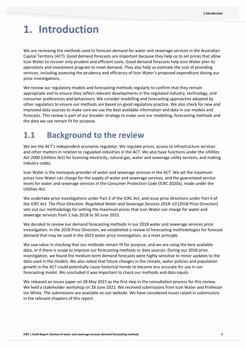
1. Introduction
We are reviewing the methods used to forecast demand for water and sewerage services in the Australian Capital Territory (ACT). Good demand forecasts are important because they help us to set prices that allow Icon Water to recover only prudent and efficient costs. Good demand forecasts help Icon Water plan its operations and investment program to meet demand. They also help us estimate the cost of providing services, including assessing the prudency and efficiency of Icon Water’s proposed expenditure during our price investigations.
We review our regulatory models and forecasting methods regularly to confirm that they remain appropriate and to ensure they reflect relevant developments in the regulated industry, technology, and consumer preferences and behaviours. We consider modelling and forecasting approaches adopted by other regulators to ensure our methods are based on good regulatory practice. We also check for new and improved data sources to make sure we use the best available information and data in our models and forecasts. This review is part of our broader strategy to make sure our modelling, forecasting methods and the data we use remain fit for purpose.
1.1 Background to the review We are the ACT’s independent economic regulator. We regulate prices, access to infrastructure services and other matters in relation to regulated industries in the ACT. We also have functions under the Utilities Act 2000 (Utilities Act) for licensing electricity, natural gas, water and sewerage utility services, and making industry codes.
Icon Water is the monopoly provider of water and sewerage services in the ACT. We set the maximum prices Icon Water can charge for the supply of water and sewerage services, and the guaranteed service levels for water and sewerage services in the Consumer Protection Code (ICRC 2020a), made under the Utilities Act.
We undertake price investigations under Part 3 of the ICRC Act, and issue price directions under Part 4 of the ICRC Act. The Price Direction: Regulated Water and Sewerage Services 2018–23 (2018 Price Direction) sets out our methodology for setting the maximum prices that Icon Water can charge for water and sewerage services from 1 July 2018 to 30 June 2023.
We decided to review our demand forecasting methods in our 2018 water and sewerage services price investigation. In the 2018 Price Direction, we established a review of forecasting methodologies for forecast demand that may be used in the 2023 water price investigation, as a reset principle.
We saw value in checking that our methods remain fit for purpose, and we are using the best available data, or if there is scope to improve our forecasting methods or data sources. During our 2018 price investigation, we found the medium-term demand forecasts were highly sensitive to minor updates to the data used in the models. We also noted that future changes in the climate, water policies and population growth in the ACT could potentially cause historical trends to become less accurate for use in our forecasting model. We concluded it was important to check our methods and data inputs.
We released an issues paper on 28 May 2021 as the first step in the consultation process for this review. We held a stakeholder workshop on 28 June 2021. We received submissions from Icon Water and Professor Ian White. The submissions are available on our website. We have considered issues raised in submissions in the relevant chapters of this report.

4
1 Introduction
ICRC | Draft Report: Review of water and sewerage services demand forecasting methods
The publication of this draft report is the second step in our consultation process for this review. Stakeholder submissions on the draft report will inform our development of the final report scheduled for release in November 2021.
We have made a draft decision to improve aspects of our forecasting methods and the data we use. If we make a final decision to change aspects of our forecasting methods and data sources, we will apply those improvements in our next price investigation to set regulated water and sewerage services prices for the regulatory period beginning on 1 July 2023.
1.2 Importance of demand forecasts Demand forecasts are an important input for setting prices
We use demand forecasts to set maximum prices for water and sewerage services so Icon Water can recover its costs of providing those services.
We use a ‘building block’ methodology to determine the prudent and efficient costs that Icon Water can recover from its customers in a regulatory period. Under the building block model, the revenue that Icon Water can earn for a regulatory period is the sum of the operating expenditure, a contribution to the cost of capital investments made over time, and allowances for forecast tax paid by the business.
This total allowed revenue is then divided by the forecast demand for each service, which includes estimates of future water usage and expected number of water and sewerage service connections, to derive a price for each service (illustrated in Figure 1). That is, Icon Water’s costs are spread over the demand to set the prices.
Figure 1. Simplified building block methodology
We need forecasts for water and sewerage services demand to set prices for individual services
We need forecasts of demand for water and sewerage services to help estimate the unit cost of providing these services (for example, the cost per kL of water). We also use demand forecasts to calculate prices that will allow Icon Water to earn enough revenue given its costs:
• Icon Water earns revenue from water services through a supply charge (per day) and a two-tier usage charge that depends on the amount of water used by a customer. Therefore, we need forecasts of water connection numbers and water usage to determine prices that will allow Icon Water to earn enough revenue to recover its costs.

5
1 Introduction
ICRC | Draft Report: Review of water and sewerage services demand forecasting methods
• Icon Water earns revenue from sewerage services through fixed supply charges. There is a fixed supply charge for residential customers and non-residential customers. There is also an additional fixed charge that applies to non-residential customers with more than two flushable fixtures. We need forecasts of sewerage installations and flushable fixtures to determine prices that will allow Icon Water to recover its costs.
• The cost of sewerage services depends on the volume of sewage that will need to be treated. Therefore, we need an estimate of sewage volumes to understand the sewage treatment costs faced by Icon Water.
Good demand forecasts ensure only prudent and efficient costs are included in setting prices
Demand forecasts help us to assess the prudency and efficiency of Icon Water’s proposed expenditure during our price investigations. Icon Water’s cost of providing the services is influenced by demand. For example, Icon Water’s infrastructure needs to be large enough to meet projected demand but not too large so that unnecessary costs are incurred. Good demand forecasts can help us assess whether Icon Water’s capital investment program and forecast operating costs are prudent and efficient. This helps us ensure that consumers pay for only those costs that are necessary to meet their demand for services.
Good demand forecasts also help Icon Water plan its operations to meet demand. For example, they improve Icon Water’s information base for its investment decisions. This helps Icon Water ensure that it incurs only those costs needed to meet demand for water and sewerage services, that is, prudent and efficient costs.
Good demand forecasts ensure consumers pay reasonable prices and Icon Water recovers its costs
Most of Icon Water’s costs are fixed. We use demand forecasts to allocate these fixed costs across the water and sewerage services that are supplied to consumers. We then add the costs that are directly related to providing services (known as variable costs). Together these costs are recovered through prices.
If demand forecasts in a regulatory period are significantly different from actual demand, prices will not reflect Icon Water’s assessed costs. If the demand forecasts are too low, the prices that we set will be too high. This means the consumers’ bills will be higher than what they should be for Icon Water to recover its costs. If the demand forecasts are too high, the prices that we set will be too low and Icon Water will not recover its prudent and efficient costs. This could affect Icon Water’s financial sustainability and its ability to keep providing water and sewerage services.
Our objective is to choose the methods that give forecasts that are likely to be closer to actual demand, so the effects of inaccurate demand forecasts on consumers and Icon Water are minimised.
We have a mechanism in place to share water demand forecasting risk between Icon Water and customers
Although our objective is to improve forecasting accuracy, predicting future water demand by its nature gives rise to the risk that actual demand may differ from forecast demand. That means the actual revenue earned by Icon Water from water sales will be higher or lower than the allowable revenue. We call this water demand risk. We have a mechanism in place to manage this demand risk (box 1.1).

6
1 Introduction
ICRC | Draft Report: Review of water and sewerage services demand forecasting methods
Box 1.1 The ‘deadband’ mechanism to share water demand risk
Our mechanism to manage water demand risk allows an adjustment at the end of the regulatory period if we find that Icon Water’s actual revenue from ACT water sales over the regulatory period is materially different from the allowable revenue. We use a materiality threshold (known as the ‘deadband’) of 6%. That means if in a regulatory period Icon Water over-recovers or under-recovers its allowed revenue from water usage charges by more than 6%, we will make an adjustment to Icon Water’s allowable revenue in the following regulatory period.
Our end of period adjustment means Icon Water can recover material under recoveries from customers and must return material over recoveries to customers during the following regulatory period. Under this approach, Icon Water bears the water demand risk up to the level of the 6% and consumers bear the risk beyond 6%. The deadband essentially shares the risk of water usage being lower or higher than forecast between Icon Water and its customers.
The ‘deadband’ was introduced during the 2008-13 regulatory period to address the risks posed by setting prices in advance of knowing actual demand. It gives Icon Water an incentive to better understand the factors driving water usage to manage the risk of lower water consumption, while limiting Icon Water’s exposure to demand risk to 6%.
We reviewed the deadband mechanism during our review of incentive mechanisms in relation to water and sewerage services and found that it results in an appropriate allocation of water demand risk between Icon Water and its customers (ICRC 2020b).
Therefore, in this review we are not considering the deadband mechanism. Rather, our focus in this review is to identify ways to improve the forecast accuracy of our model to reduce the demand risk.
1.3 Scope of the review In this review, we will determine the water and sewerage services forecasting methods and data to be used in the next water price investigation, which is likely to start in late 2021.
We intend to review the current forecasting methods and data sources based on a set of assessment criteria (described in section 1.7). We will consider the pros and cons of alternative forecasting approaches compared to the current approach. We will identify appropriate forecasting methods and data sources based on the assessment criteria.
7
1 Introduction
ICRC | Draft Report: Review of water and sewerage services demand forecasting methods
We intend to review the methods for six components of water and sewerage services demand that we need to determine the maximum water and sewerage prices in the ACT. The components are:
1.3.1 Water services demand components
1. Total water abstractions from dams
Forecast volume of dam abstractions in each year is used to estimate the billed water sales in the ACT (discussed below) and to estimate the annual Water Abstraction Charge paid by Icon Water to the ACT Government.
2. Billed water sales at Tier 1 and Tier 2
Icon Water sells water at two price tiers. Tier 1 rate applies to water usage up to 50kL per quarter and Tier 2 rate applies to water usage above that amount. Water sales are forecast for these two tiers separately.
3. Total number of water service connections
Total number of water service connections in each year are forecast to estimate Icon Water’s revenue from water supply charges in each year.
1.3.2 Sewerage services demand components
4. Total number of sewerage services connections
Total number of sewerage service connections in each year are forecast to estimate Icon Water’s revenue from sewerage supply charges in each year.
5. The number of additional billable fixtures
A flushable fixture is either a toilet, urinal or other fixture with a flushing cistern or flush valve. Non-residential customers with more than two flushable fixtures pay a separate fee for each additional fixture. Total number of additional billable fixtures is forecast to estimate Icon Water’s revenue from supply charges for these fixtures.
6. Sewage volumes
Forecasts of sewage volumes are required to estimate sewage treatment costs, which are then used to set Icon Water’s sewerage prices.
1.4 Purpose of the draft report There are two reasons for this draft report. The first is to inform stakeholders of our draft decisions on the methods and data we will use to forecast demand for water and sewerage services. The second is to allow stakeholders an opportunity to provide feedback on our draft decisions, which will inform our final report.
1.5 Our role and objectives Under the ICRC Act, we have the following objectives as set out in sections 7 and 19L of the ICRC Act (box 1.2).
8
1 Introduction
ICRC | Draft Report: Review of water and sewerage services demand forecasting methods
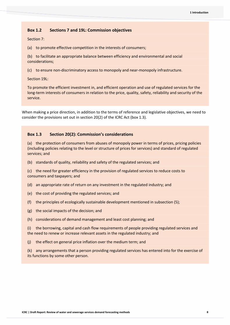
Box 1.2 Sections 7 and 19L: Commission objectives
Section 7:
(a) to promote effective competition in the interests of consumers;
(b) to facilitate an appropriate balance between efficiency and environmental and social considerations;
(c) to ensure non-discriminatory access to monopoly and near-monopoly infrastructure.
Section 19L:
To promote the efficient investment in, and efficient operation and use of regulated services for the long-term interests of consumers in relation to the price, quality, safety, reliability and security of the service.
When making a price direction, in addition to the terms of reference and legislative objectives, we need to consider the provisions set out in section 20(2) of the ICRC Act (box 1.3).
Box 1.3 Section 20(2): Commission’s considerations
(a) the protection of consumers from abuses of monopoly power in terms of prices, pricing policies (including policies relating to the level or structure of prices for services) and standard of regulated services; and
(b) standards of quality, reliability and safety of the regulated services; and
(c) the need for greater efficiency in the provision of regulated services to reduce costs to consumers and taxpayers; and
(d) an appropriate rate of return on any investment in the regulated industry; and
(e) the cost of providing the regulated services; and
(f) the principles of ecologically sustainable development mentioned in subsection (5);
(g) the social impacts of the decision; and
(h) considerations of demand management and least cost planning; and
(i) the borrowing, capital and cash flow requirements of people providing regulated services and the need to renew or increase relevant assets in the regulated industry; and
(j) the effect on general price inflation over the medium term; and
(k) any arrangements that a person providing regulated services has entered into for the exercise of its functions by some other person.
9
1 Introduction
ICRC | Draft Report: Review of water and sewerage services demand forecasting methods
1.6 Technical advice on forecasting methods We have engaged the consultancy firm Marsden and Jacob Associates to provide expert technical advice for this review.
In stage 1, the consultant compared alternative forecasting approaches to the current approach and advised that we maintain the current forecasting approach. The consultant’s stage 1 report was published with our issues paper.
In stage 2, the consultant has developed advice on how the current forecasting approach could be improved. We have considered its advice in developing this draft report. The consultant’s stage 2 report is in appendix 4.
1.7 Our approach to this review
1.7.1 Assessment criteria for the review
We are proposing to use a set of criteria to assess our demand forecasting methods.
Having assessment criteria will promote consistency in decision making when assessing different models. In developing the assessment criteria, we considered the pricing principles in our final report on regulated water and sewerage services prices for 2018-23 (ICRC 2018). These pricing principles are reproduced in appendix 1 for ease of reference. We developed these pricing principles during our tariff structure review 2016-17 (ICRC 2017a).
The assessment criteria that we are proposing to use in this review are:
• Economic logic, transparency and replicability. This means that the model should be based on well-established theory, assumptions used in the model should be clearly documented and can be tested, modelling should be based on well-established statistical methods, and stakeholders should reasonably understand the processes involved and be able to replicate the results.
• Predictive ability. This is to review how accurate the model is in predicting actual outcomes.
• Flexibility. The model’s ability to accommodate changing circumstances such as change in climate and water policies.
• Regulatory stability. The forecasting methodology needs to be relatively stable over time to give stakeholders certainty. The methods should only be updated where there is sufficient evidence that the change would increase the accuracy of the predictions.
• Simplicity. The methods should be simple for consumers to understand and straightforward for the utility service provider to implement.
We consider that these criteria will address our legislative objectives and the matters that we are required to consider under section 20(2) of the ICRC Act. The allowable revenue we determine based on the forecast demand, must promote efficient investment in, and the efficient operation and use of, regulated services for the long-term interests of consumers.
These criteria promote confidence in our forecasting methods among the regulated business, consumers, investors, and other stakeholders.
The criteria ensure that the methods are simple, and stakeholders can replicate the models. Improved predictive ability will provide Icon Water confidence that it can earn sufficient revenue to recover its costs, and it will encourage Icon Water to make prudent and efficient investment decisions. Regulatory stability
10
1 Introduction
ICRC | Draft Report: Review of water and sewerage services demand forecasting methods
will promote efficient investment in, and use of, the relevant services because it gives investors the confidence to make investments in long-lived water assets.
1.7.2 Icon Water’s view on the assessment criteria
In the issues paper, we sought stakeholder comments on our assessment criteria for this review. Icon Water submitted that it supports the assessment criteria (Icon Water 2021).
On the criterion of transparency and replicability, Icon Water’s view is that the model should use reliable and publicly available data to forecast water demand. For example, Icon Water said that wherever possible proprietary data, subscription data, or other third-party data should not be used because there is a risk that those data could be discontinued or modified. We agree that the data used in the model should be publicly available, widely accepted and sourced from a reputable organisation. We also consider that the model should use updated data that accounts for more recent observations.
Icon Water’s view is that predictive ability should be assessed based on how accurate the forecast is, on average, over the regulatory period rather than in every year of the regulatory period. Icon Water reasoned that was because demand forecasts are used to set prices for it to recover its efficient revenue over a five-year regulatory period. Icon Water says it is not feasible for a model to accurately predict changing weather conditions from year to year.
We accept that the predictive ability of a model should be evaluated, on average, over the five-year regulatory period. However, we also consider that if there is significant annual variability between forecast and actual water demand, we should investigate if aspects of the forecasting model could be improved to reduce the variability. For example, a comparison of forecast and actual dam abstractions data for the first three years of the regulatory period shows that the difference in:
• 2018-19 was +6% (actual abstractions were greater than forecast)
• 2019-20 was +10% (actual abstractions were greater than forecast)
• 2020-21 was -2% (actual abstractions were less than forecast)
Although, on average, over the three years the actual abstractions were 5% greater than forecast, the significant annual variability in the first two years due to drier than average weather conditions cannot be overlooked. We have identified aspects of the forecasting model that can be improved to better account for weather-related variability (see section 4.2 of this draft report).
On flexibility, Icon Water notes that there are different ways in which a model can accommodate changing circumstances. Some changes can be accommodated within the model itself. However, some events may require alternative treatments, for example, a post-model adjustment that involves modifying the output of the model to account for an expected future shock to demand. We accept there are different ways for a model to be flexible and the most appropriate way will depend on the specific circumstances.
Icon Water agrees that regulatory stability is an important element of the demand forecasting methodology. Icon Water’s view is that methodological changes should only be made where there is strong evidence that the benefits will outweigh the costs and risks. Since this review is about demand forecasting methods, we consider that the methods should only be updated where there is sufficient evidence that the change would increase the accuracy of the predictions. We used this test in the 2018 water and sewerage services price investigation, and accepted Icon Water’s proposed forecasting model, rather than retaining the Industry Panel model. We did that because the evidence indicated that Icon Water’s proposed model increased forecast accuracy.
On the criterion of simplicity, Icon Water’s view is that the high-level approach to the forecasting method should be intuitive for the community to understand the main drivers of water demand. For example, the
11
1 Introduction
ICRC | Draft Report: Review of water and sewerage services demand forecasting methods
model used to forecast dam abstractions is capable of being understood by the general community because the relationship between weather and water demand can be intuitively understood.
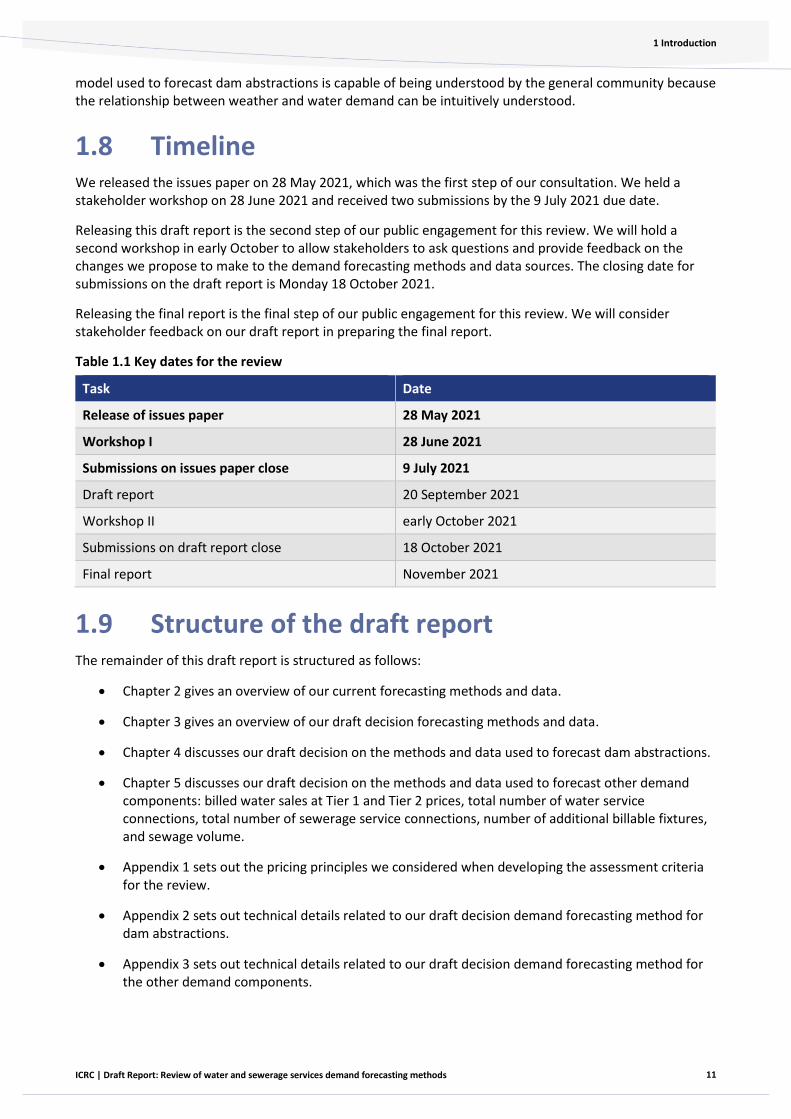
1.8 Timeline We released the issues paper on 28 May 2021, which was the first step of our consultation. We held a stakeholder workshop on 28 June 2021 and received two submissions by the 9 July 2021 due date.
Releasing this draft report is the second step of our public engagement for this review. We will hold a second workshop in early October to allow stakeholders to ask questions and provide feedback on the changes we propose to make to the demand forecasting methods and data sources. The closing date for submissions on the draft report is Monday 18 October 2021.
Releasing the final report is the final step of our public engagement for this review. We will consider stakeholder feedback on our draft report in preparing the final report.
Table 1.1 Key dates for the review
Task Date
Release of issues paper 28 May 2021
Workshop I 28 June 2021
Submissions on issues paper close 9 July 2021
Draft report 20 September 2021
Workshop II early October 2021
Submissions on draft report close 18 October 2021
Final report November 2021
1.9 Structure of the draft report The remainder of this draft report is structured as follows:
• Chapter 2 gives an overview of our current forecasting methods and data.
• Chapter 3 gives an overview of our draft decision forecasting methods and data.
• Chapter 4 discusses our draft decision on the methods and data used to forecast dam abstractions.
• Chapter 5 discusses our draft decision on the methods and data used to forecast other demand components: billed water sales at Tier 1 and Tier 2 prices, total number of water service connections, total number of sewerage service connections, number of additional billable fixtures, and sewage volume.
• Appendix 1 sets out the pricing principles we considered when developing the assessment criteria for the review.
• Appendix 2 sets out technical details related to our draft decision demand forecasting method for dam abstractions.
• Appendix 3 sets out technical details related to our draft decision demand forecasting method for the other demand components.

12
1 Introduction
ICRC | Draft Report: Review of water and sewerage services demand forecasting methods
• Appendix 4 is the consultant’s stage 2 report.
• Appendix 5 gives an overview of the forecasting approaches used in other Australian jurisdictions.

13
2 Overview of our current forecasting methods and data
ICRC | Draft Report: Review of water and sewerage services demand forecasting methods
2. Overview of our current forecasting methods and data
2.1 Forecasting water services demand We apply a top-down approach to forecast water sales in the ACT. There are three steps, which are described below and presented in Figure 2.
Step 1
The first step is to forecast the volume of water abstractions from Icon Water’s dams. We start with dam abstractions because they are a good indicator of billed water sales and data are available on a daily frequency. Dam abstractions are also used to assess Icon Water’s operating and capital costs, and to estimate the water abstraction charge.
The dam abstractions model uses climate related data on rainfall, temperature and evaporation, which are available on a daily frequency. We use climate variables because we consider that there is a direct relationship between water consumption and climate variables. For example, there will be low demand for water on rainy days, and high demand for water on hot days and when evaporation rate is high. The changing water demand due to weather conditions will have an impact on water abstractions from Icon Water’s dams.
We need information on what future climate conditions will look like. In our 2018 water and sewerage services price investigation, we used four separate climate scenarios (driest, dry, medium and wet) developed by the South Eastern Australian Climate Initiative (SEACI). We used these scenarios to develop future climate scenarios for rainfall and evaporation. However, the future scenario for temperature was developed based on the historical trend. We used the average of dam abstractions forecasts from the different climate scenarios because it is not possible to accurately predict the actual climate conditions.
A stable relationship between water demand and climate variables will ensure reliable forecasts. For example, we know that water demand is high during summer months. But changes in consumer behaviour can affect the relationship between water sales and climate variables. Such behavioural changes can include the use of more water efficient appliances, installation of more water efficient garden watering systems, and water recycling systems.
During the millennium drought, many consumers changed their behaviour in response to water restrictions that were in place in the ACT from 2002 to 2010. We found that water demand in the period during, and after, water restrictions increased less in response to warmer and drier weather compared to in the period before restrictions. A new relationship between water sales and climate variables developed in 2006 which has remained stable since then. Therefore, we use data from 2006 to forecast dam abstractions.
The forecast model also uses data on water connection numbers, because water demand increases when there are more consumers. Future water connection numbers are estimated based on the past growth trend in the connection numbers.
The model we currently use to forecast dam abstractions is a multivariate Autoregressive Integrated Moving Average (ARIMA) model. ARIMA models are used for forecasting variables that are measured over time, like dam abstractions.

14
2 Overview of our current forecasting methods and data
ICRC | Draft Report: Review of water and sewerage services demand forecasting methods
Step 2
In step 2, we forecast the share of dam abstractions that will be sold to ACT consumers. Icon Water sells some of its dam abstractions to Queanbeyan city council and part of dam abstractions includes water leakages, water lost due to theft, and unaccounted water due to metering errors. We look at the historical shares of dam abstractions sold to ACT consumers to forecast the future share.
Step 3
Icon Water sells water at two price tiers. So, in step 3, total ACT water sales is split into Tier 1 and Tier 2. The split is based on the historical relationship between the average amount of water consumed by each customer and the proportion of Tier 1 sales.
Figure 2. Simplified representation of the current approach for forecasting water services demand
Source: Our analysis based on Icon Water (2021)
2.2 Forecasting sewerage services demand Like the forecast for water connection numbers, the forecasts for sewerage installations and billable fixtures are made based on the past growth trend.
Sewage volumes are forecast based on a range of factors including average sewage volume per resident, population growth, groundwater flow into the sewerage system, and climate conditions.
2.3 Matters raised in the issues paper Our issues paper sought feedback from stakeholders on whether improvements could be made to the forecasting methods and data used to forecast the components of water and sewerage services demand.
We identified specific issues for stakeholder comments relating to issues like how to incorporate future changes in the climate, water policies, population growth and consumer behaviour. For example, we sought stakeholders’ feedback on:
Climate variables
• Temperature• Rainfall• Evaporation
Combined with future climate scenarios
Temperature Rainfall & Evaporation
Past trend SEACI climate scenarios
Dam abstractions
Daily
Water connection numbers
ARIMA Model
Billed water sales
Forecasting water services demand: current approach
Medium Dry DriestWet
Since 2006
ACT water sales
Tier 1Tier 2
Step 1
Step 2
Step 3
Forecast based on past growth trend (based on historical relationships)
15
2 Overview of our current forecasting methods and data
ICRC | Draft Report: Review of water and sewerage services demand forecasting methods
• other more suitable data sources to account for climate change
• if, and how, the sustainable diversion limit should be incorporated into the model. It limits the amount of water that can be taken from the rivers for towns, industries, and farmers in the Murray-Darling basin
• whether to use ACT population projections to forecast connection numbers
• how to incorporate changes in consumer behaviour and what sort of data to use
• any changes in the forecasting methods needed to improve the stability of the forecasts
• whether we should change the frequency of data used in the model (from daily data to monthly data) to improve the model’s ability to account for climate change
• whether the model used to forecast dam abstractions remains appropriate
• whether the methods and data used to forecast other demand components—billed water sales at Tier 1 and Tier 2 prices, total number of water service connections, total number of sewerage service connections, number of additional billable fixtures, and sewage volume—remain appropriate.
2.4 Overview of submissions to the issues paper We received submissions from Icon Water and Professor Ian White. Icon Water commented on a range of issues and Professor White commented on the specific issue of climate change data.
We also heard stakeholder views at the workshop held on 28 June 2021.
We have considered stakeholders’ comments in developing our draft decisions, which are discussed in chapters 3 to 5 of this report.

16
3 Overview of our draft decisions
ICRC | Draft Report: Review of water and sewerage services demand forecasting methods
3. Overview of our draft decisions
This chapter gives an overview of our draft decisions on forecasting methods and data sources. Further details are given in chapters 4 and 5 and in the appendices.
3.1 Forecasting water services demand We will maintain the top-down approach to forecast water sales in the ACT. The starting point will be to forecast the volume of water abstractions from Icon Water’s dams, which will be used to estimate water sales in the ACT.
We will retain the current dam abstractions forecasting method (ARIMA model). We consider that the model meets our assessment criteria. It uses information on climate and customer numbers to provide reliable forecasts. The model is replicable and transparent and provides regulatory stability.
We will continue using climate variables (temperature, rainfall and evaporation) as drivers of water demand. We will retain the current approach of using future climate scenarios to forecast dam abstractions. We have made a draft decision to use a different data source for future climate scenarios. For the next regulatory period, we will use the NSW and ACT Regional Climate Modelling (NARCLiM) climate change projections, which are now widely accepted and provide a single, up-to-date source for localised climate change projections.
We will continue to use water connection numbers to forecast dam abstractions. Our draft decision is to forecast water connection numbers based on ACT population projections rather than past growth trends in connection numbers. This approach allows the model to account for demographic changes that could not be captured by looking at a past trend.
We will continue to use data from July 2006 to account for the change in consumer behaviour that occurred during the millennium drought. The evidence shows that water consumption behaviour in the ACT has remained stable since then.
The current model does not account for the sustainable diversion limit (SDL) which limits the amount of water that can be taken from the rivers for towns, industries and farmers in the Murray-Darling basin. We have developed principles to adjust the output of the model for certain types of changes that affect water and sewerage services demand and may apply them in the next price investigation to consider any changes to the SDL.
The current model uses daily observations to forecast dam abstractions. Our draft decision is to use weekly data to forecast dam abstractions. We found that the form of model based on weekly data improves the predictive performance of the model. This position is subject to further refinement of the model specification and stakeholder feedback.
We will retain the current methods to forecast ACT water sales and billed water sales at Tier 1 and Tier 2. Our draft decision is to add more recent years’ data to the existing dataset to forecast billed water sales and the Tier 1 and Tier 2 split.
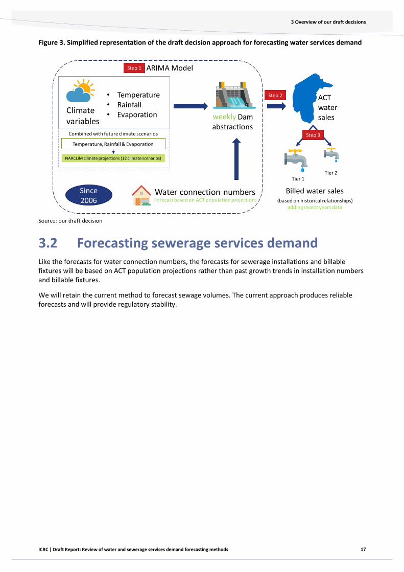
Figure 3 is a simplified representation of the draft decision approach to forecast water services demand. The changes compared to our current approach are shown in green.
17
3 Overview of our draft decisions
ICRC | Draft Report: Review of water and sewerage services demand forecasting methods
Figure 3. Simplified representation of the draft decision approach for forecasting water services demand
Source: our draft decision
3.2 Forecasting sewerage services demand Like the forecasts for water connection numbers, the forecasts for sewerage installations and billable fixtures will be based on ACT population projections rather than past growth trends in installation numbers and billable fixtures.
We will retain the current method to forecast sewage volumes. The current approach produces reliable forecasts and will provide regulatory stability.
Climate variables
• Temperature• Rainfall• Evaporation
Combined with future climate scenarios
Dam abstractionsweekly
Water connection numbers
ARIMA Model
Billed water sales
Forecasting water services demand: draft decision approach
Since 2006
ACT water sales
Tier 1Tier 2
Step 1
Step 2
Step 3
Forecast based on ACT population projections (based on historical relationships)adding recent years data
Temperature, Rainfall & Evaporation
NARCLiM climate projections (12 climate scenarios)

18
4 Forecasting dam abstractions
ICRC | Draft Report: Review of water and sewerage services demand forecasting methods
4. Forecasting dam abstractions
We apply a top-down approach to forecast water sales in the ACT. The starting point is to forecast the volume of water abstractions from Icon Water’s dams, which is used to estimate water sales in the ACT.
This chapter discusses our draft decisions on the method and data used to forecast dam abstractions. Section 4.1 is about the approach to forecast dam abstractions. Section 4.2 is about the functional form of the model and data used to forecast dam abstractions.
4.1 Dam abstractions forecasting approach
Summary of the draft decision
We will retain the current method, which is a multivariate Autoregressive Integrated Moving Average (ARIMA) model, to forecast dam abstractions.
We consider that the ARIMA model meets our assessment criteria. It uses information on climate and customer numbers to provide reliable forecasts. The model is replicable and transparent and provides regulatory stability. Our consultant compared alternative forecasting approaches to the ARIMA approach and advised that the ARIMA approach is appropriate and fit for purpose (Marsden Jacobs Associates 2021a). Icon Water submitted that the ARIMA model remains appropriate (Icon Water 2021).
Our draft decision is therefore to retain the ARIMA model. We have identified several components of the ARIMA model that can be improved, and these are discussed in section 4.2.
Details of this draft decision
The ARIMA model satisfies our assessment criteria
Our assessment of the ARIMA model against the assessment criteria is as follows:
Criterion 1: Economic logic, transparency and replicability
We forecast dam abstractions because it serves multiple purpose. Dam abstractions are a good indicator of water sales in the ACT. They are also needed to assess Icon Water’s operating and capital costs, and to estimate the water abstraction charge.
We use the ARIMA approach because it is used for forecasting variables that are measured over time, like dam abstractions. It is an approach that looks at the relationships between dam abstractions and the factors that influence dam abstractions such as climate and customer numbers over time and makes a forecast assuming these relationships will hold in the future. The ARIMA approach allows adjusting these relationships if we believe historical data will not be a useful predictor on its own.
The ARIMA model is a transparent and replicable method. It is based on well-established statistical processes and is a widely used forecasting approach. The assumptions used in the ARIMA model are clearly documented and modelling can be done using well-established procedures.
We assessed forecasting models used in other jurisdictions and found that there is no single well-accepted forecasting model. Different forecasting methods are used in other jurisdictions. For example, Sydney Water uses a panel data approach, Hunter Water and Melbourne Water use end-use modelling, and SA
19
4 Forecasting dam abstractions
ICRC | Draft Report: Review of water and sewerage services demand forecasting methods
Water uses a simple regression model. Although the forecasting methods are different across jurisdictions, the main drivers of water demand used in these jurisdictions—climate variables, population and water conservation measures—are common.
Utilities in other jurisdictions appear to use the demand forecasting methodology most suited to the type of data they have access to and the purpose of demand forecasts.
In the case of Sydney Water and Hunter Water, which use panel data regression and end use approaches respectively, demand forecasts are used in their regulatory submissions for setting prices as well as for water conservation reporting.
Melbourne Water contracts the bulk of its supply through three large customers, which in turn distribute water to the end user. As each of these customers does their own demand forecasting, Melbourne Water can make its demand forecasts based on the usage of its three largest customers.
SA Water uses an econometric model based on the historical water usage it has access to, and forecasts demand based on relationships observed between water demand and its drivers after the millennium drought.
Appendix 5 summarises forecasting methods used in the other jurisdictions.
Criterion 2: Predictive ability
The evidence available to us indicates that the ARIMA model provides reliable forecasts. We compared dam abstraction forecasts made in our 2018 water price investigation with actual volumes for the first three years of the current regulatory period. We found the model has reasonable predictive ability because the average difference over that three-year period is less than 5%.
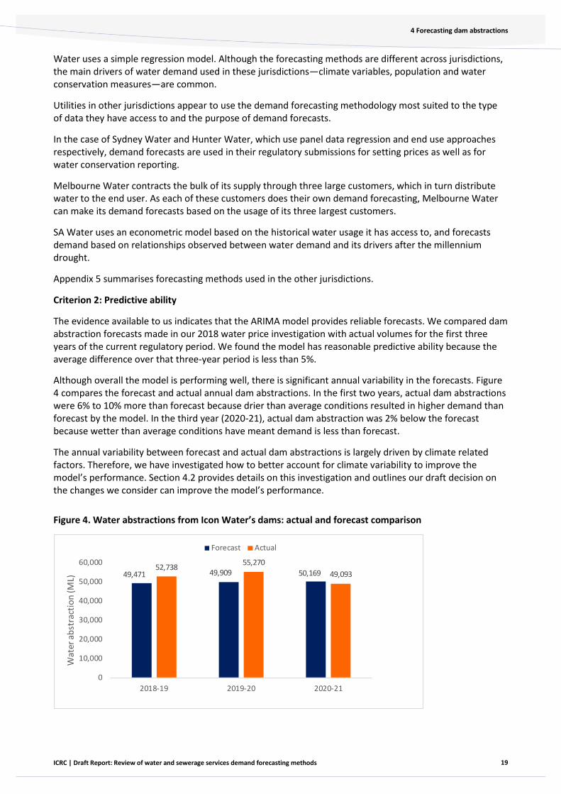
Although overall the model is performing well, there is significant annual variability in the forecasts. Figure 4 compares the forecast and actual annual dam abstractions. In the first two years, actual dam abstractions were 6% to 10% more than forecast because drier than average conditions resulted in higher demand than forecast by the model. In the third year (2020-21), actual dam abstraction was 2% below the forecast because wetter than average conditions have meant demand is less than forecast.
The annual variability between forecast and actual dam abstractions is largely driven by climate related factors. Therefore, we have investigated how to better account for climate variability to improve the model’s performance. Section 4.2 provides details on this investigation and outlines our draft decision on the changes we consider can improve the model’s performance.
Figure 4. Water abstractions from Icon Water’s dams: actual and forecast comparison
49,471 49,909 50,16952,738
55,270
49,093
0
10,000
20,000
30,000
40,000
50,000
60,000
2018-19 2019-20 2020-21
Wat
er a
bst
ract
ion
(ML)
Forecast Actual
20
4 Forecasting dam abstractions
ICRC | Draft Report: Review of water and sewerage services demand forecasting methods
Source: our analysis based on data from Icon Water
Criterion 3: Flexibility
Flexibility refers to the model’s ability to accommodate changing circumstances such as changes in climate and water policies. The current ARIMA model has flexibility to respond to certain changes in circumstances. It accounts for short-term fluctuations in weather conditions and the seasonal impact on water demand. It also accounts for step changes in water demand, for example, it accounts for the sustained step-change in water use in the ACT that we noted had occurred following the millennium drought (ICRC 2015). This step change reflected changes in consumer behaviour in response to the water restrictions that were imposed during the millennium drought, where consumers installed drought tolerant gardens and water efficient appliances to conserve water and lower their water bills.
We consider that the model is flexible and that its performance can be improved by making modifications to account for the impact of climate changes on water demand, such as by considering up to date climate data sources. The post model adjustments that can be applied to the ARIMA model also provide flexibility. These modifications are discussed in section 4.2.
Criterion 4: Regulatory stability
We consider that the forecasting methodology needs to be relatively stable over time to give stakeholders certainty. We also consider that the methods should only be updated where there is sufficient evidence that the change would increase the accuracy of the predictions.
Retaining the ARIMA model will provide regulatory stability because we currently use the ARIMA model to forecast water demand and stakeholders are familiar with the modelling approach. Our consultant assessed alternative models and advised us that on balance ARIMA model is preferred. The evidence available to us indicates that the ARIMA model provides reliable forecasts. It can also be modified to improve its performance. The other modelling approaches that the consultant reviewed are more complex to implement, due to the requirement to observe water demand of set group of consumers over time and then develop estimation methods to generalise the observed data.
Criterion 5: Simplicity
Our view is that the ARIMA model is objective, transparent and relatively straightforward for the utility service provider to implement. The data on bulk water dam abstractions, rainfall and temperature that are required to implement the model are readily available. The method can be implemented using well-established methodologies using standard statistical software. The model is based on the relationship between weather and water demand, which can be intuitively understood.
ARIMA model is preferred over other approaches
Our consultant compared the performance of the ARIMA approach and 3 other approaches against our assessment criteria. The alternative approaches that were considered are:
• Panel data: A data set based on surveying the same panel of people over time and observing how their responses change.
• End use modelling: Water usage is estimated by observing water demand of different customer groups such as residential houses, residential units and non-residential customers, and aggregating their usage to produce demand forecasts.
• Historical average: Demand is forecast using a base level of historic usage adjusted for estimates of customer and population growth.
The ARIMA model that we use for dam abstractions performed better against the assessment criteria than the other approaches that were considered.
21
4 Forecasting dam abstractions
ICRC | Draft Report: Review of water and sewerage services demand forecasting methods
Our view is that ARIMA approach is transparent and reproducible and is suitable for producing medium to long-term forecasts.
The consultant advised that the ARIMA approach is simpler to implement compared to the panel data approach. Our view is that although the ARIMA approach may not be as flexible as the panel data approach, the ARIMA model that we use is flexible enough to accommodate changing circumstances as noted above. For this reason, we consider it appropriate to identify ways to improve the performance of the existing ARIMA approach, which are discussed in section 4.2.
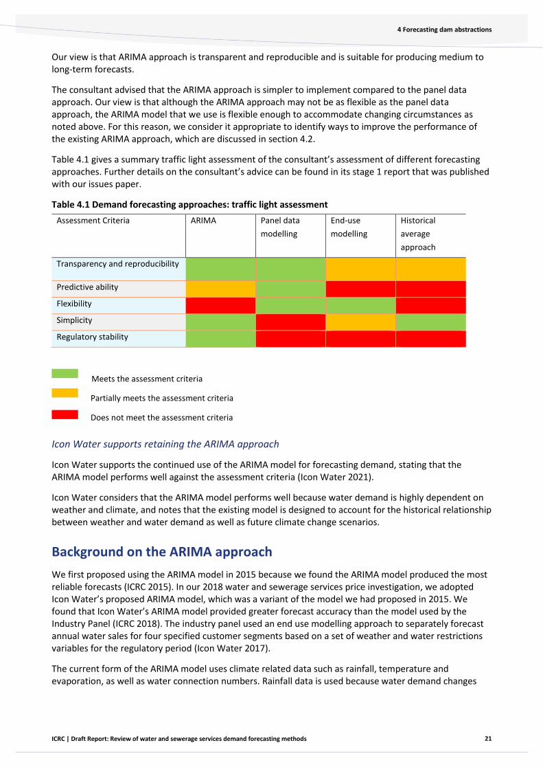
Table 4.1 gives a summary traffic light assessment of the consultant’s assessment of different forecasting approaches. Further details on the consultant’s advice can be found in its stage 1 report that was published with our issues paper.
Table 4.1 Demand forecasting approaches: traffic light assessment
Assessment Criteria ARIMA Panel data
modelling
End-use
modelling
Historical
average
approach
Transparency and reproducibility
Predictive ability
Flexibility
Simplicity
Regulatory stability
Meets the assessment criteria
Partially meets the assessment criteria
Does not meet the assessment criteria
Icon Water supports retaining the ARIMA approach
Icon Water supports the continued use of the ARIMA model for forecasting demand, stating that the ARIMA model performs well against the assessment criteria (Icon Water 2021).
Icon Water considers that the ARIMA model performs well because water demand is highly dependent on weather and climate, and notes that the existing model is designed to account for the historical relationship between weather and water demand as well as future climate change scenarios.
Background on the ARIMA approach
We first proposed using the ARIMA model in 2015 because we found the ARIMA model produced the most reliable forecasts (ICRC 2015). In our 2018 water and sewerage services price investigation, we adopted Icon Water’s proposed ARIMA model, which was a variant of the model we had proposed in 2015. We found that Icon Water’s ARIMA model provided greater forecast accuracy than the model used by the Industry Panel (ICRC 2018). The industry panel used an end use modelling approach to separately forecast annual water sales for four specified customer segments based on a set of weather and water restrictions variables for the regulatory period (Icon Water 2017).
The current form of the ARIMA model uses climate related data such as rainfall, temperature and evaporation, as well as water connection numbers. Rainfall data is used because water demand changes
22
4 Forecasting dam abstractions
ICRC | Draft Report: Review of water and sewerage services demand forecasting methods
with the amount of rainfall, with less demand for water on rainy days and during rainy periods. Temperature data is used because water demand changes with temperature, with more demand on hot days and during hot periods. The model uses evaporation data which is likely due to higher irrigation requirements for plants as they dry when evaporation is higher. Water connection numbers are included because water demand increases when there are more consumers (ICRC 2017b).
4.2 Functional form of ARIMA model and data used to forecast dam abstractions
Summary of the draft decision
We consider that the current model is fit for purpose and performing well. The changes we are proposing will future proof the model to adapt to a more dynamic and uncertain environment, especially where climate change is concerned.
We will continue using climate variables (temperature, rainfall and evaporation) as drivers of water demand. We will retain the current approach of using future climate scenarios to forecast dam abstractions. We have made a draft decision to use a different data source for informing these future climate scenarios. For the next regulatory period, we will use the NSW and ACT Regional Climate Modelling (NARCLiM) climate change projections, which are now widely accepted and provide a single, up-to-date source for localised climate change projections.
We will continue to use water customer numbers to forecast dam abstractions. We have accepted Icon Water’s suggestion to change the method used to forecast water customer numbers. The method will be based on ACT population projections rather than past growth trends in connection numbers. This approach allows the ARIMA model to account for demographic changes that could not be captured by looking at a past trend.
We will continue to use data from July 2006 to account for the change in consumer behaviour that occurred during the millennium drought. The evidence shows that water consumption behaviour in the ACT has remained stable since then.
The current ARIMA model does not account for the sustainable diversion limit (SDL) which limits the amount of water that can be taken from the rivers for towns, industries and farmers in the Murray-Darling basin. We have developed principles to adjust the output of the model (‘post-model adjustment principles’) and may apply them in the next price investigation if necessary to account for the impact of any changes in the SDL on water demand.
The current model uses daily observations for climate and dam abstractions. Our draft decision is to use weekly data because we found this improves the model’s predictive ability. This position is subject to further refinement of the model specification.
Climate variables
We will continue using climate variables as drivers of water demand but use a new data source to develop future climate scenarios
Our draft decision is to continue to use climate variables because there is a direct relationship between water consumption and climate conditions given by rainfall, evaporation and temperature.
Developing an understanding of what future climate conditions will look like is important to forecast dam abstractions. We will retain the current approach to develop future climate scenarios by adjusting historical
23
4 Forecasting dam abstractions
ICRC | Draft Report: Review of water and sewerage services demand forecasting methods
climate data by climate change projections developed by reputed external agencies. Box 4.1 outlines the current approach.
Our draft decision is to use NARCLiM climate change projections. NARCLiM is a NSW Government led partnership that provides high resolution climate change projections across NSW. The partnership began in 2011 and now includes the NSW, ACT and South Australian Governments and the Climate Change Research Centre at the University of NSW.
NARCLiM will replace the climate change projections data that, for the current regulatory period, were sourced from the South Eastern Australian Climate Initiative (SEACI). Our consultant’s advice is also to use the NARCLiM database (Marsden Jacob Associates 2021b).
Box 4.1 Current approach to develop future climate scenarios
To forecast dam abstractions, we need to understand what the conditions for rainfall, evaporation and temperature over the forecast period would be. However, climate variables are difficult to predict, especially over a 5-to-6-year period, as is required by the ARIMA model.
In our 2018 water and sewerage services price investigation, future climate scenarios were developed using the following process.
1. We considered historical daily rainfall, evaporation and temperature dating back to 1965. These data were split into successive time periods of 6.5 years each, which was chosen because during the 2018 investigation dam abstractions were forecast for 6.5 years to June 2023.
2. The average data for those time periods was calculated to establish the reference climate scenario for rainfall, evaporation and temperature, which included average daily data for temperature, rainfall and evaporation for 6.5 years.
3. To develop future climate scenarios for rainfall and evaporation, we used four future climate change scenarios (dry, driest, wet and medium) developed by SEACI. Each SEACI scenario gives the average impact on rainfall and evaporation by season for an increase in global warming by one degree Celsius. This impact is expressed in percentage terms and is called ‘adjustment factor’. For each climate change scenario, the relevant adjustment factors were applied to the rainfall and evaporation data in the reference climate scenario. This process gave adjusted daily rainfall and evaporation data, which represented the expected rainfall and evaporation conditions for the forecast period.
4. To develop future climate scenario for temperature, the trend in daily maximum temperature was estimated using daily data from June 1965 to March 2017. We assumed this trend will continue over the 6.5 year period. The maximum daily temperature in the reference climate scenario was adjusted to reflect this trend which represented the expected temperature conditions for the forecast period.
Our preferred climate change projections data source is NARCLiM
We compared NARCLiM data source against two other climate change projections data sources: SEACI (which was used in the last price investigation) and the Australian Community Climate and Earth System Simulator—Seasonal (ACCESS-S), which was suggested by Professor Ian White in his submission to our Issues Paper (Table 4.2).

24
4 Forecasting dam abstractions
ICRC | Draft Report: Review of water and sewerage services demand forecasting methods
Table 4.2 Comparison of climate change projections data sources
NARCLiM SEACI ACCESS-S
Acceptance Icon Water, Sydney Water, IPART, ACT Government, NSW Government, SA Government
Murray-Darling Basin Authority
Bureau of Meteorology (BoM), CSIRO
Updates Projections developed in 2014 and updated in 2020 to reflect the release of new global climate change projections
Projections developed in 2012
Projections are continuously developed (the model is dynamic)
Geographic coverage ACT specific at 10km resolution
South-Eastern Australia Australia wide, but available at 60km resolution
Climate variables coverage
Temperature, rainfall, evaporation
Rainfall, evaporation Rainfall, temperature
Projections future period
Projections available from 2020 to 2100
Not specified. Projections developed for 1 and 2 degrees of global warming.
Seasonal outlook
Source: our analysis based on information from NARCLiM: https://climatechange.environment.nsw.gov.au/climate-projections-for-NSW/About-NARCliM; ACCESS-S: http://www.bom.gov.au/climate/ahead/about/model/access.shtml; SEACI: http://www.seaci.org/research/futureProjections.html
We found that NARCLiM data source is widely used, including for regulated price setting. For example, Sydney Water used it in its demand forecasts for the 2020–24 regulatory period, which was accepted by Independent Pricing and Regulatory Tribunal (IPART). Icon Water uses it for network planning; the ACT Government uses it in its climate adaptation planning; and the NSW Government uses it to inform strategic planning initiatives relating to infrastructure, transport emergency risk assessment and regional water strategies.
NARCLiM provides highly localised ACT specific data at a 10km resolution, which is relevant for forecasting ACT specific water demand whereas SEACI and ACCESS-S have a broader geographic coverage.
Using NARCLiM will ensure consistency in developing future climate scenarios for all three climate variables—temperature, rainfall and evaporation—that we use. This is because NARCLiM will be a single source to adjust all three climate variables. SEACI and ACCESS-S only provide projections for two of the three variables.
NARCLiM projections are updated periodically as new global climate change projections are released. For example, NARCLiM projections were first developed in 2014 and updated in 2020 to incorporate more recent global climate models released by the Intergovernmental Panel on Climate Change. This periodic updating will ensure that NARCLiM data set will remain relevant for years to come, promoting stability within our approach. In comparison, the SEACI data source was developed in 2012 and is currently 10 years old. The ACCESS-S data source is updated continuously, but it provides short-term projections which are not useful for a 5-year regulatory period.
More information on NARCLiM climate change projections is given in appendix 2.
25
4 Forecasting dam abstractions
ICRC | Draft Report: Review of water and sewerage services demand forecasting methods
Stakeholders identified different data sources for developing future climate scenarios
Icon Water supports using the NARCLiM data source because it reflects recent climate modelling and said that it meets the assessment criteria of transparency and replicability because the information is publicly available (Icon Water 2021).
Professor Ian White submitted that warming seas around the globe have created more volatile weather events, such as the intense storms and flooding experienced by Sydney in early 2021. He considered that our current approach does not account for increasing climate volatility. Professor White considers that ACCESS-S is the most reliable data source for seasonal projections (Professor Ian White 2021).
We agree with Professor White that there is scope to improve our current model to better account for climate volatility. In adopting the NARCLiM data source, which was updated in 2020 to incorporate more recent global climate models released by the Intergovernmental Panel on Climate Change, we expect that the model will be able to account for increasing climate volatility. In this draft decision, we have identified specific improvements to the model: use of low frequency data (weekly instead of daily) to better capture variability in weather conditions. These are discussed later in this section.
We note Professor White’s comment about ACCESS-S being the most reliable data source for seasonal climate events. However, as discussed above, we consider that NARCLiM data source is more suited to our needs.
Professor White also said that the current 6% deadband is conservative and that it should be increased. The consideration of deadband is outside the scope of this review. We reviewed the deadband mechanism during our review of incentive mechanisms in relation to water and sewerage services and found that it results in an appropriate allocation of water demand risk between Icon Water and its customers (ICRC 2020b). In that review, we said that we will consider the deadband threshold during the next water and sewerage services price investigation.
Sustainable diversion limit
We have developed principles for adjusting the model output and may apply them in the next price investigation
The current ARIMA model does not account for the sustainable diversion limit (SDL) which limits the amount of water that can be taken from the rivers for towns, industries and farmers in the Murray-Darling basin.
The evidence shows that the SDL is unlikely to have any immediate impact on water demand in the ACT. SDLs came into effect on 1 July 2019 and represent the maximum long-term annual average quantities of water that can be taken on a sustainable basis from Basin water resources. The ACT’s annual actual take has been about half of the annual permitted take (Figure 5). This evidence shows that potential reductions in the SDL are unlikely to have medium term impacts on dam abstractions in the ACT.
We have developed principles to adjust the output of the model and may apply them in the next price investigation to account for the impact of any changes to the SDL on water demand. Box 4.2 sets out the principles.

26
4 Forecasting dam abstractions
ICRC | Draft Report: Review of water and sewerage services demand forecasting methods
Figure 5. ACT annual permitted take and actual take (GL)
Source: our analysis based on data from https://www.mdba.gov.au/sites/default/files/pubs/appendix-2-surface-water-sustainable-diversion-limit-accounts-7-years.pdf; https://www.mdba.gov.au/sites/default/files/pubs/murray-darling-basin-sustainable-diversion-limit-compliance-outcomes-2019-20-report.pdf
Annual permitted take limits change in a manner that it is difficult to forecast within the model
The SDL and annual permitted take change from year to year as they are based on climate, water trade, usage patterns and development of infrastructure, making it difficult to forecast future limits and their impact on dam abstractions.
Under the SDL framework, credits and debits can be accumulated. A credit is recorded for a given year if actual take was less than the permitted take. A debit is recorded if actual take was more than the permitted take. Each year the credits/debits are added to those from the previous year and so can build up over time. The ACT’s balance at the end of the first year of SDL was +22.3GL.1 The accumulation of credits/debits can make it challenging to forecast future limits and their impact on dam abstractions.
—————
1 https://www.mdba.gov.au/sites/default/files/pubs/murray-darling-basin-sustainable-diversion-limit-compliance-outcomes-2019-20-report.pdf
50.9 50.949.3
52.3
46.4
52.754.0 53.7
27.5 27.625.8
28.9
25.1
30.431.8 31.4
2012-13 2013-14 2014-15 2015-16 2016-17 2017-18 2018-19 2019-20
Annual permitted take (GL) Annual actual take (GL)

27
4 Forecasting dam abstractions
ICRC | Draft Report: Review of water and sewerage services demand forecasting methods
An appropriate approach is to adjust the model output to account for the impact of SDL changes
Policy impacts can have several uncertainties associated with them such as implementation, specific details of the policy and its impact on water demand. If these details are uncertain, it can be difficult to incorporate the impact into the forecast method.
The post-model adjustment process typically involves adjusting the output of the model to account for the impact of a policy change on forecast demand. The process provides flexibility in capturing the impact of a policy change and is transparent.
We will apply post-model adjustment principles to consider the impact of SDL on water demand
Currently, the SDL is unlikely to have medium term impacts on water demand in the ACT. Whether SDLs will be a future constraint will depend on the changes to the limits and the availability of new information such as actual water use figures. We will consider a model adjustment process to consider the impact of SDL as per our post-model adjustment principles, outlined in box 4.2.
Box 4.2 Post-model adjustment principles
Post-model adjustments are used to adjust the output of the model to account for future impacts of events. These adjustments should adhere to a set of principles:
• The event is outside the control of the regulated business (such as government policy change).
• The event is specific and its impact on water demand is direct and certain (such as water restrictions, forcing demand for water to decrease).
• There is a reasonable and transparent way to measure the impact and adjust the model to account for the event (for example, adjusting gas demand forecasts based on the switching rate of customers from gas to electricity).
The Australian Energy Regulator (AER) recently used a post-model adjustment approach to account for future impacts of climate change policy on gas demand. The determination for EvoEnergy used a model adjustment to consider factors that were not present within historical data, in this case, a reduction in gas consumption arising from the ACT Government’s Climate Change Strategy 2020–25, which aims for net zero emissions by 2045 (AER 2021).
The implementation of this policy is a specific event that was outside of EvoEnergy’s control and has a clear impact on gas demand as consumers are encouraged to switch from gas to electricity. To estimate the impact of the policy, the AER considered data from the incremental impact of the ACT Energy Efficiency Improvement Scheme (EEIS), which provides incentives for gas customers to switch to electricity. The AER found the switching rate caused by the EEIS was a reasonable basis for forecasting customer responses to the policy in future (AER 2021).
Icon Water supports the use of post-model adjustments to account for future changes to the SDL
Icon Water submitted that it is challenging to model the impact of future policy changes and that the SDL will not have any immediate impacts over the foreseeable future. Icon Water suggested using post-model adjustments to account for any changes to the SDL in the future.

28
4 Forecasting dam abstractions
ICRC | Draft Report: Review of water and sewerage services demand forecasting methods
Background information on SDL
The ACT is in the Murrumbidgee River catchment, which feeds into the Murray–Darling River system. In 2019, federal and state Murray-Darling Basin water ministers established an annual limit called the SDL as a major change in water management policy. SDLs limit how much water, on average, can be used in the Murray-Darlin Basin by towns and communities, farmers, and industries, to keep the rivers and environment healthy.
The ACT has obligations under the Murray–Darling Basin Agreement and Murray–Darling Basin Plan to comply with the SDL (EPSDD 2019). The SDL introduced a new water accounting and compliance framework in the Murray–Darling Basin, replacing the previous ‘Cap on Surface Water Diversions’ compliance framework.
The Murray-Darling Basin Authority assesses and monitors Basin state compliance with SDLs. The Basin Plan requires Basin state governments to manage the use of water within SDLs. Complying with SDLs is based on the concepts of permitted take and actual take.
• Permitted take is an annualised expression of the SDL. It is the volume of water that is expected to be extracted during a water year under the SDL.
• Actual take is how much water was extracted in a given water year.
Although the SDL framework began in July 2019, Basin states have been trialling the SDL framework since 2012.
The SDL puts a limit on the amount of water abstractions from Icon Water’s dams. As our current model forecasts dam abstractions, the limit given by the SDL could constrain the output of the model.
Changes in consumer behaviour
We will retain the current approach to account for changes in consumer behaviour
We will continue to use data from July 2006 to account for the change in consumer behaviour that occurred during the millennium drought. The evidence shows that water consumption behaviour in the ACT has remained stable since then.
During the millennium drought, many consumers changed their behaviour in response to water restrictions that were in place in the ACT from 2002 to 2010 (box 4.3). We found that water demand in the period during and after water restrictions increased less in response to warmer and drier weather compared to in the period before restrictions. A new relationship between water sales and climate variables developed in about July 2006 which has remained stable since then (ICRC 2015). Icon Water agreed with this conclusion in its 2018 submission (Icon Water 2018). Therefore, we use data since July 2006 to forecast dam abstractions.
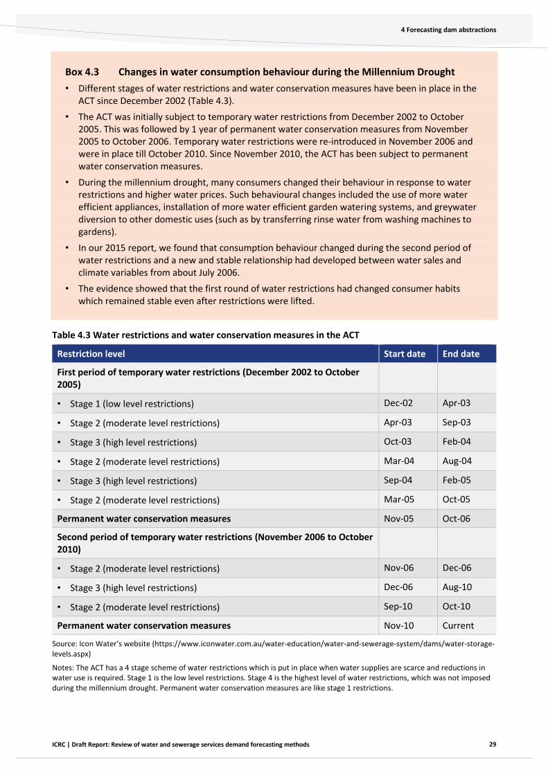
29
4 Forecasting dam abstractions
ICRC | Draft Report: Review of water and sewerage services demand forecasting methods
Box 4.3 Changes in water consumption behaviour during the Millennium Drought
• Different stages of water restrictions and water conservation measures have been in place in the ACT since December 2002 (Table 4.3).
• The ACT was initially subject to temporary water restrictions from December 2002 to October 2005. This was followed by 1 year of permanent water conservation measures from November 2005 to October 2006. Temporary water restrictions were re-introduced in November 2006 and were in place till October 2010. Since November 2010, the ACT has been subject to permanent water conservation measures.
• During the millennium drought, many consumers changed their behaviour in response to water restrictions and higher water prices. Such behavioural changes included the use of more water efficient appliances, installation of more water efficient garden watering systems, and greywater diversion to other domestic uses (such as by transferring rinse water from washing machines to gardens).
• In our 2015 report, we found that consumption behaviour changed during the second period of water restrictions and a new and stable relationship had developed between water sales and climate variables from about July 2006.
• The evidence showed that the first round of water restrictions had changed consumer habits which remained stable even after restrictions were lifted.
Table 4.3 Water restrictions and water conservation measures in the ACT
Restriction level Start date End date
First period of temporary water restrictions (December 2002 to October 2005)
• Stage 1 (low level restrictions) Dec-02 Apr-03
• Stage 2 (moderate level restrictions) Apr-03 Sep-03
• Stage 3 (high level restrictions) Oct-03 Feb-04
• Stage 2 (moderate level restrictions) Mar-04 Aug-04
• Stage 3 (high level restrictions) Sep-04 Feb-05
• Stage 2 (moderate level restrictions) Mar-05 Oct-05
Permanent water conservation measures Nov-05 Oct-06
Second period of temporary water restrictions (November 2006 to October 2010)
• Stage 2 (moderate level restrictions) Nov-06 Dec-06
• Stage 3 (high level restrictions) Dec-06 Aug-10
• Stage 2 (moderate level restrictions) Sep-10 Oct-10
Permanent water conservation measures Nov-10 Current
Source: Icon Water’s website (https://www.iconwater.com.au/water-education/water-and-sewerage-system/dams/water-storage-levels.aspx)
Notes: The ACT has a 4 stage scheme of water restrictions which is put in place when water supplies are scarce and reductions in water use is required. Stage 1 is the low level restrictions. Stage 4 is the highest level of water restrictions, which was not imposed during the millennium drought. Permanent water conservation measures are like stage 1 restrictions.
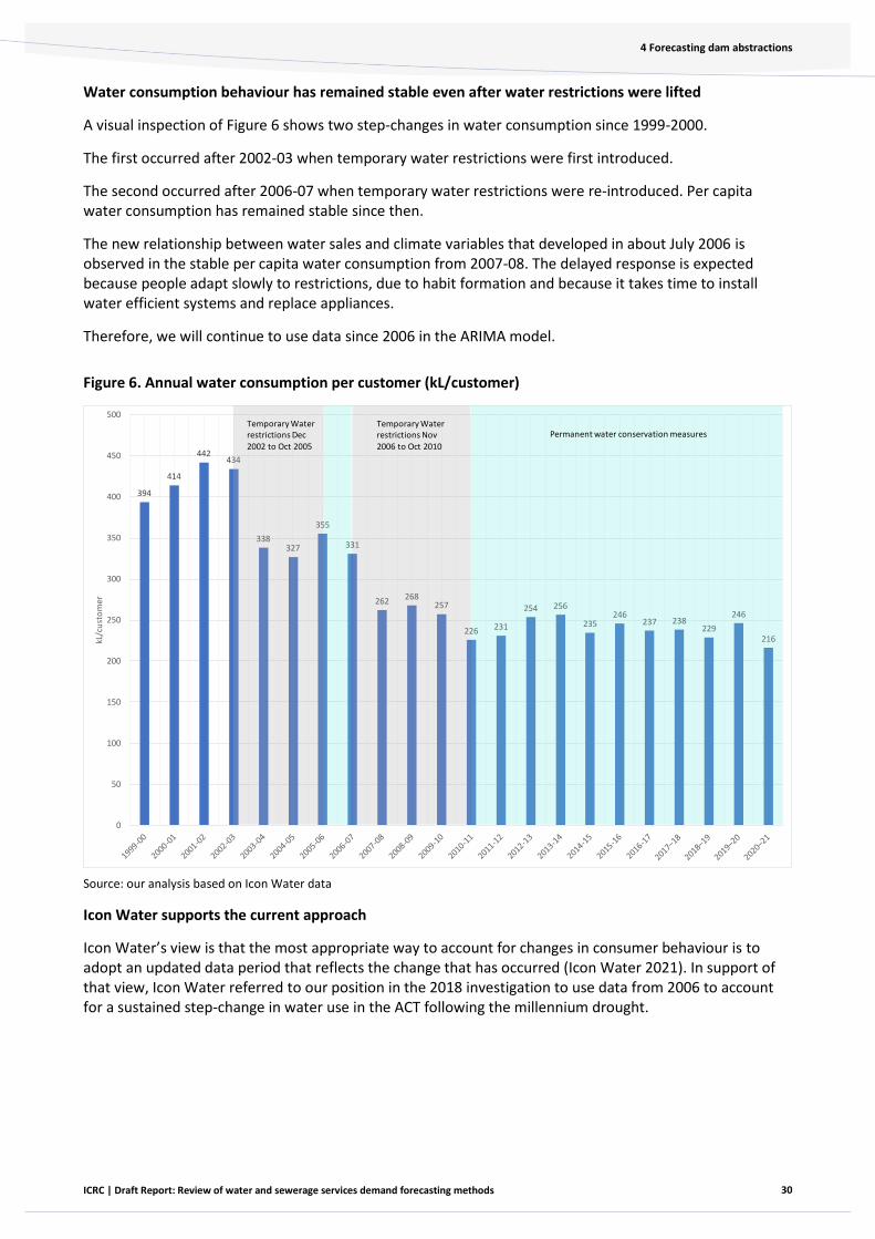
30
4 Forecasting dam abstractions
ICRC | Draft Report: Review of water and sewerage services demand forecasting methods
Water consumption behaviour has remained stable even after water restrictions were lifted
A visual inspection of Figure 6 shows two step-changes in water consumption since 1999-2000.
The first occurred after 2002-03 when temporary water restrictions were first introduced.
The second occurred after 2006-07 when temporary water restrictions were re-introduced. Per capita water consumption has remained stable since then.
The new relationship between water sales and climate variables that developed in about July 2006 is observed in the stable per capita water consumption from 2007-08. The delayed response is expected because people adapt slowly to restrictions, due to habit formation and because it takes time to install water efficient systems and replace appliances.
Therefore, we will continue to use data since 2006 in the ARIMA model.
Figure 6. Annual water consumption per customer (kL/customer)
Source: our analysis based on Icon Water data
Icon Water supports the current approach
Icon Water’s view is that the most appropriate way to account for changes in consumer behaviour is to adopt an updated data period that reflects the change that has occurred (Icon Water 2021). In support of that view, Icon Water referred to our position in the 2018 investigation to use data from 2006 to account for a sustained step-change in water use in the ACT following the millennium drought.
394
414
442434
338327
355
331
262 268257
226 231
254 256
235246
237 238229
246
216
0
50
100
150
200
250
300
350
400
450
500
kL/c
ust
om
er
Temporary Waterrestrictions Dec
2002 to Oct 2005
Temporary Waterrestrictions Nov
2006 to Oct 2010
Permanent water conservation measures
31
4 Forecasting dam abstractions
ICRC | Draft Report: Review of water and sewerage services demand forecasting methods
Demographic changes
We will use ACT population projections rather than the past growth trend to forecast customer numbers
We will continue to use water customer numbers to forecast dam abstractions because water demand increases when there are more consumers.
Currently future customer numbers are estimated based on the past growth trend in customer numbers. Our draft decision is to change the method used to forecast customer numbers. The method will be based on the ACT Government population projections to provide a forward-looking forecast of customer numbers. This approach allows the ARIMA model to account for demographic changes that could not be captured by looking at a past trend.
It is now acknowledged that the Covid-19 pandemic has affected the drivers of ACT’s population growth, and the ACT’s population growth is expected to be lower than what was expected before the pandemic (ACT Government 2021). We will review our position to ensure that the ACT population projections we use to forecast Icon Water’s customer numbers account for the impact of the pandemic.
Further details of the new method to forecast customer numbers are given in section 5.4 and appendix 3.
Population projections provide forward looking forecasts
The current approach of extrapolating previous trends in Icon Water’s customer numbers may not account for changing demographic trends, such as increasing population density as more people in the ACT live in apartments rather than detached homes.
The ACT Government’s population projections account for population growth including from migration and uses assumptions based on the ACT Government’s long-term land release program and expected development activity, which can influence the number of future water customers and hence water demand.
We note the ACT Government’s population projections are being updated to account for the effect of Covid-19, and the updated projections are expected to be published in the second half of 2021.2 We will monitor this development to ensure that the ACT population projections we use account for the impact of the pandemic.
Icon Water supports the current approach
Icon Water has stated a preference for continuing to use water connection numbers in the ARIMA model as a proxy for population (Icon Water 2021).
Icon Water observed a strong historical relationship between the number of water connections and the ACT population. It noted that connection numbers can be highly influenced by factors such as government and private property development, and that future growth in connections may be different from the past growth rate. It suggested using the ACT Government population projections to forecast water connection numbers.
Background on demographic changes
Demographic changes can reflect changes in population growth and may also relate to changes in average age and family structure. These changes may result in changes in the mix of housing types (for example, the proportion of freestanding houses and apartments) that will have direct effects on water demand. A family living in a detached house with a backyard is likely to consume more water than the same sized family living
—————
2 https://www.treasury.act.gov.au/snapshot/demography/act
32
4 Forecasting dam abstractions
ICRC | Draft Report: Review of water and sewerage services demand forecasting methods
in an apartment. An increase in the average age of the ACT community, coupled with a move to downsizing, could lead to a greater share of apartments or townhouses with small outdoor areas, which tend to use less water for outdoor uses.
The ACT Government population projections3 are based on the Australian Bureau of Statistics Population by Age and Sex, Regions of Australia (2017) and assumptions about fertility, mortality and migration. The projections also use assumptions based on the ACT Government’s long-term land release program and expected development activity.
Stability of model outputs
In our 2018-23 water price investigation, we found the demand forecasts changed significantly when Icon Water added 11 months of data from April 2017 to February 2018 for their revised pricing proposal. The forecast water abstractions increased by 1.3 % to 1.5 % in each year over the 2018-23 regulatory period. This indicates that the demand forecasts produced by the current ARIMA model are sensitive to minor updates to the data used in the model.
Icon Water agrees that more recent data are given greater weight in the ARIMA model. However, it noted that the cumulative increase was 1.4% over the 5-year regulatory period. Icon Water considers that the change in demand forecasts due to addition of more recent data is a function of the ARIMA model. It noted that when additional data is added to a forecasting model, it should be expected that the forecasts will change because the dynamic nature of the model ensures that the model satisfies the ‘flexibility’ criterion and does not remain static over time. Icon Water suggests retaining the current approach.
We agree with Icon Water’s submission and consider the current method to update the model to account for more recent data is appropriate.
Variability of model outputs and data frequency
We will use weekly data, subject to further refinement of the model
The current model uses daily observations for climate and dam abstractions.
Our draft decision is to use weekly data to forecast dam abstractions. Our consultant has found that using weekly data improves the predictive performance of the model compared to daily or monthly observations.
We consider that using weekly data is intuitively sound because daily data are influenced by factors that are not relevant to forecast dam abstractions over longer horizons, for example, water consumption habits of customers on a day-to-day basis (such as using more water on the weekends than weekdays). Such day-to-day differences are not relevant to forecasting dam abstractions over a 5-year regulatory period.
Our draft decision is subject to further refinement of the model specification, which will depend on our final position on the draft decisions set out in this report.
Weekly data improves model performance
Our consultant’s analysis shows that weekly data performs better than daily or monthly data.
Our consultant compared the forecasting accuracy of the current daily data model with a model based on weekly and monthly observations. It also considered additional variables to better capture extreme weather conditions, for example, number of days where daily temperature exceeded 30 degrees within the
—————
3 ACT Population Projection: 2018 to 2058

33
4 Forecasting dam abstractions
ICRC | Draft Report: Review of water and sewerage services demand forecasting methods
previous week (month) and number of days where daily rainfall exceeded 1 mm within the previous week (month).
The consultant assessed forecasting accuracy by estimating well known measures of Root Mean Square Percentage Error (RMSPE) and the Mean Absolute Percent Error (MAPE). RMSPE and MAPE measure the average difference (squared or absolute, respectively) between the yearly forecast and actual values. In the 2018 investigation, Icon Water used these measures to compare the performance of its form of ARIMA model against the form we identified in our 2015 report.
The consultant found that (Table 4.4):
• Forecasting accuracy improved significantly with weekly data relative to daily data, as both MAPE and RMSPE values are more than halved. There is little effect from adding extra weather variables.
• With monthly data, forecasting accuracy improved compared to daily data, and improved further when extra weather variables are added into the model.
The data in Table 4.4 show that when using weekly data (in the benchmark model), the difference between the annual forecast and actual volume was the lowest: 1.6% to 1.9% on average (lower difference means better performance). This contrasts with daily data where the average difference was the highest: 3.8% to 4.3% on average. The monthly data was in the middle with an average difference of 2.1% to 2.9%.
Table 4.4 Forecasting accuracy using daily, weekly and monthly data
Daily data Weekly data Monthly data
Benchmark Augmented Benchmark Augmented Benchmark Augmented
MAPE 3.80% 3.71% 1.61% 1.63% 3.14% 2.06%
RMSPE 4.27% 4.19% 1.86% 1.87% 4.01% 2.87%
Source: Marsden Jacob Associates (2021b)
Note: Benchmark – without additional weather variables, Augmented – with additional weather variables
Why weekly and monthly data perform better than daily data in forecasting over longer horizons
The nature of daily observations is that they can be affected by fluctuations that are irrelevant over a longer horizon. For example, they may be affected by outlier events on the day, such as an extreme hot day, which may not represent normal weather conditions. Daily observations are also heavily influenced by intra-week variation. For example, models based on daily data require taking into account the impact of the day of the week on total abstractions such as weekends vs weekdays, which are not relevant to forecasting dam abstractions over longer horizon. The information in daily data that is not relevant for longer term forecasting is called ‘noise’.
The noise in daily observations may make it harder to identify trends or cycles in weather conditions that are relevant to forecasting dam abstractions over longer horizon.
The noise in daily observations introduces a degree of error in the forecasting process for models based on daily observations. These errors will compound over time. So, the longer the forecast horizon, the greater will be the compounding error effect from daily observations. Our forecast horizon is 5 years, which is the length of the regulatory period.
In comparison, intra-week seasonal variations and outlier events are averaged out with weekly and monthly data, thus avoiding forecasting errors caused by noise in the data. Also, low frequency data (weekly or monthly) are better suited to show trends and cycles in weather conditions.
34
4 Forecasting dam abstractions
ICRC | Draft Report: Review of water and sewerage services demand forecasting methods
Why weekly data performs better than monthly data
A potential limitation with using monthly observations is that there are fewer observations to estimate the relationship between dam abstractions and their drivers such as climate and customer numbers: 12 monthly observations compared to 52 weekly observations in a year. There is some degree of information loss with monthly data relative to weekly data. Information loss will affect the forecasting accuracy of models that use monthly data.
This information loss would make weekly data perform better than monthly data, as shown in Table 4.4.
The information loss may be overcome by adding explanatory variables that capture new information. The consultant’s analysis shows that the performance of monthly data improved when new explanatory variables designed to capture extreme weather events were added. However, this may increase the complexity of the model.
Icon Water’s view on data frequency
Icon Water submitted that it was not aware of any evidence that using low-frequency data would improve the predictive ability of the ARIMA model. It expressed concern that using monthly data would require significant effort to recalibrate the model to identify the best-fit model specification.
We consider the process of recalibrating the model to identify the best-fit model specification is a normal process. We did that in 2015 when we proposed using the ARIMA model. Icon Water also did that process in 2018 when it proposed using its form of ARIMA model, compared to our form of the ARIMA model.
Background on forecast variability
We consider that if there is significant annual variability between forecast and actual water demand, we should investigate whether aspects of the forecasting model could be improved to reduce the variability.
For example, a comparison of forecast and actual dam abstractions data for the first three years of the regulatory period (Figure 4) shows that the difference in:
• 2018-19 was +6% (actual abstractions were greater than forecast)
• 2019-20 was +10% (actual abstractions were greater than forecast)
• 2020-21 was -2% (actual abstractions were less than forecast)
Although, on average, over the three years the actual abstractions were 5% greater than forecast, the significant annual variability in the first two years due to drier than average weather conditions cannot be overlooked. As discussed in this section of the report, we have identified aspects of the forecasting model that can be improved to better account for weather-related variability.

35
4 Forecasting dam abstractions
ICRC | Draft Report: Review of water and sewerage services demand forecasting methods
Our draft decision on the form of the ARIMA Model
Table 4.5 summarises our draft decision on the drivers of water demand we will use, the reason for selecting them, and the data sources we will use to estimate them.
Table 4.5 Summary of variables to be used under our draft decision on the form of the model
Drivers of water demand
Reasoning Data source
Maximum temperature (degrees Celsius)
Temperature data is used because water demand changes with temperature, with more demand during hot periods
Canberra Airport weather station data reported by the Bureau of Meteorology (BoM); NARCLiM climate change projections data
Rainfall (mm) Rainfall data is used because water demand changes with the amount of rainfall, with less demand for water during rainy periods.
Rainfall data at Canberra Airport reported by BoM; NARCLiM climate change projections data
Evaporation rate (mm) High evaporation rates are related to higher irrigation requirements for plants/gardens as they dry.
Evaporation data for Burrinjuck Dam reported by BoM; NARCLiM climate change projections data
Water customer numbers
An increase in customers will increase demand for water.
Icon Water (historical customers data); Australian Bureau of Statistics (historical population data); ACT Government population projections data
Dam abstractions (ML) Represents historical dam abstractions and allows us to identify a relationship between dam abstractions over time.
Icon Water (historical data); this is a function of the ARIMA model and is calculated using the model.
Seasonality To capture the effect of different volumes of water use in different seasons such as high water use in summer months and low water use in winter months.
Calculated using a mathematical formula to capture annual seasonal pattern.
Unforeseeable events Accounts for the impact of unforeseeable and unobserved events on water demand (such as bushfires).
This is a function of the ARIMA model and is calculated using the model.
Our consultant’s analysis shows that the weekly data model has better statistical properties than the daily data model.
For example, the estimated effect of the additional variables included in the weekly data model to capture the effect of extreme weather conditions on dam abstractions is as expected. The estimated coefficient for the variable ‘number of days where maximum daily temperature exceeded 30 °C’ within the previous week is 9.88: it shows that for every additional day when daily temperature exceeded 30 °C, dam abstractions increase on average by 10ML, keeping all other variables constant.
The weekly data model also shows that the impact on dam abstractions is more than proportionate when the temperature threshold is increased to 35 °C. The estimated coefficient for the variable ‘number of days where maximum daily temperature exceeded 35 °C’ is 24.34: it means that for every additional day when daily temperature exceeded 35 °C, dam abstractions increased on average by 24ML, keeping all other variables constant.
In contrast, the daily data model shows an unexpected result for extreme hot days. The estimated coefficient for the variables that are designed to consider the effect on water demand of days when
36
4 Forecasting dam abstractions
ICRC | Draft Report: Review of water and sewerage services demand forecasting methods
temperature exceeded 35 °C or 40 °C has a negative sign (-2.86 to -0.42): this would mean days when the temperature exceeded 35 °C or 40 °C are associated with lower dam abstractions, keeping all other variables constant. This counterintuitive result is caused by the noise (very high volatility) in daily observations.
Our consultant’s analysis also shows that the estimated coefficients for the weekly model have signs that are consistent with expectations. For example, in the model, evaporation is included in linear form (amount of evaporation) and non-linear form (squared value and square root value of the amount of evaporation). In such cases, the effect of evaporation on dam abstractions is considered by looking at the coefficient estimates for the linear and non-linear forms as well as the amount of evaporation. The consultant’s analysis shows that the relationship between dam abstractions and evaporation is like a U-shape: as evaporation increases, dam abstractions increase but this increase is less than proportionate.
The detailed estimation results are presented in the appendix 2 and in the consultant’s report in appendix 4.
Our next steps to finalise the model specification
After we have finalised our decisions set out in this draft report, taking into account information and views provided by stakeholders, our consultant will make final refinements to the model to ensure it is statistically sound and reliable.
Based on our consultant’s advice, we will finalise the model to ensure it best fits the data. The final model specification will establish the final statistical form of the drivers of water demand listed in Table 4.5: whether to use squared values, square root values and how many ‘lags’ to use, which is commonly used in ARIMA models where it is assumed that the forecast value of a variable is dependent upon past observations of that variable (for example, using past dam abstractions to forecast future dam abstractions).
37
5 Forecasting other demand components
ICRC | Draft Report: Review of water and sewerage services demand forecasting methods
5. Forecasting other demand components
This chapter discusses our draft decision on the methods and data used to forecast the other water and sewerage services demand components, which are:
• total ACT water sales
• billed water sales at Tier 1 and Tier 2
• total number of water service connections, total number of sewerage service connections, number of billable fixtures
• sewage volume.
5.1 Summary of the draft decisions
We will retain the current method to forecast ACT water sales and billed water sales at Tier 1 and Tier 2. The current approach produces reliable forecasts and will provide regulatory stability. The only change we will make is to add more recent years’ data to the existing dataset to forecast billed water sales and the Tier 1 and Tier 2 split.
We have accepted Icon Water’s suggestion to change the method to forecast water and sewerage services connection numbers and number of billable fixtures. The method will be based on ACT population projections rather than past growth trends in connection numbers and billable fixtures. We consider ACT population projections are a better indicator of the future connection numbers and billable fixtures. There is a stable relationship between ACT population numbers and these demand components, so using population forecasts will capture future demographic changes and provide a better indicator to forecast connection numbers and billable fixtures.
We will retain the current method to forecast sewage volumes. The current approach produces reliable forecasts and will provide regulatory stability.
5.2 Total ACT water sales
We will retain the current method to forecast total ACT water sales
We will retain our current method to forecast total ACT water sales based on the historical shares of dam abstractions sold to ACT consumers. Box 5.1 outlines the current method.
We consider it appropriate to retain the current method because there is a stable relationship between ACT water sales and dam abstractions, and the method produces reliable forecasts. Therefore, the current method meets our assessment criteria of predictive ability and regulatory stability.
There is a stable relationship between ACT water sales and dam abstractions
On average, ACT water sales accounts for about 80% to 90% of the volume of water abstractions from Icon Water’s dams, and this ratio has been stable for over two decades (Figure 7). The balance of water abstractions is accounted for by Queanbeyan consumption and water losses due to leaking pipes, theft, and metering errors.

38
5 Forecasting other demand components
ICRC | Draft Report: Review of water and sewerage services demand forecasting methods
Figure 7. Ratio of annual ACT water sales to annual dam abstractions
Source: our analysis based on Icon Water data
The current method produces reliable forecasts
We compared forecast ACT water sales made in our 2018 water price investigation with actual ACT water sales for the first three years of the current regulatory period. We found that the forecasts are reasonably accurate because the average difference over the period is 2%. Figure 8 shows the forecast and actual ACT water sales for the first three years of the current regulatory period.
Figure 8. Total ACT water sales: actual and forecast comparison
Source: our analysis based on data from Icon Water
-
0.10
0.20
0.30
0.40
0.50
0.60
0.70
0.80
0.90
1.00
41,903 42,193 42,40141,80845,795
41,472
0
5,000
10,000
15,000
20,000
25,000
30,000
35,000
40,000
45,000
50,000
2018-19 2019-20 2020-21
AC
T w
ater
sal
es (
ML)
Forecast
Actual
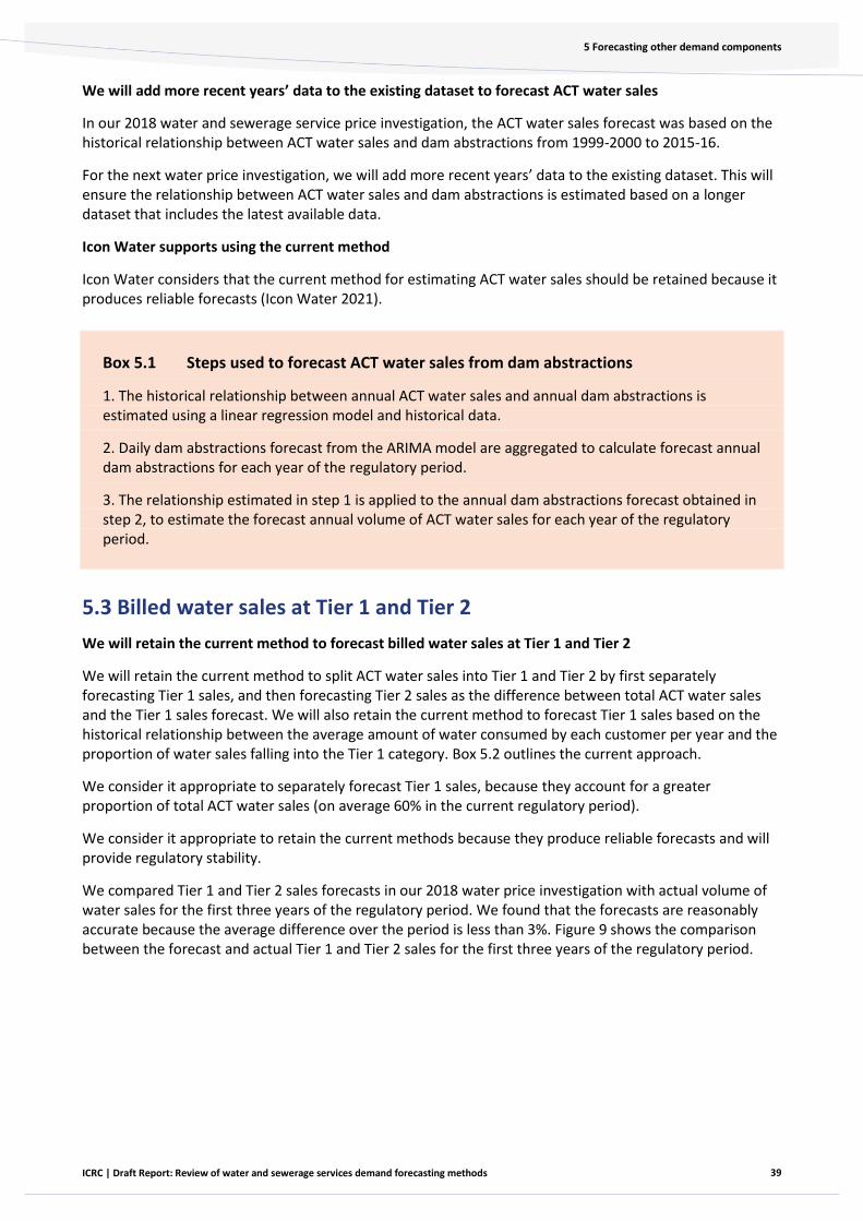
39
5 Forecasting other demand components
ICRC | Draft Report: Review of water and sewerage services demand forecasting methods
We will add more recent years’ data to the existing dataset to forecast ACT water sales
In our 2018 water and sewerage service price investigation, the ACT water sales forecast was based on the historical relationship between ACT water sales and dam abstractions from 1999-2000 to 2015-16.
For the next water price investigation, we will add more recent years’ data to the existing dataset. This will ensure the relationship between ACT water sales and dam abstractions is estimated based on a longer dataset that includes the latest available data.
Icon Water supports using the current method
Icon Water considers that the current method for estimating ACT water sales should be retained because it produces reliable forecasts (Icon Water 2021).
Box 5.1 Steps used to forecast ACT water sales from dam abstractions
1. The historical relationship between annual ACT water sales and annual dam abstractions is estimated using a linear regression model and historical data.
2. Daily dam abstractions forecast from the ARIMA model are aggregated to calculate forecast annual dam abstractions for each year of the regulatory period.
3. The relationship estimated in step 1 is applied to the annual dam abstractions forecast obtained in step 2, to estimate the forecast annual volume of ACT water sales for each year of the regulatory period.
5.3 Billed water sales at Tier 1 and Tier 2
We will retain the current method to forecast billed water sales at Tier 1 and Tier 2
We will retain the current method to split ACT water sales into Tier 1 and Tier 2 by first separately forecasting Tier 1 sales, and then forecasting Tier 2 sales as the difference between total ACT water sales and the Tier 1 sales forecast. We will also retain the current method to forecast Tier 1 sales based on the historical relationship between the average amount of water consumed by each customer per year and the proportion of water sales falling into the Tier 1 category. Box 5.2 outlines the current approach.
We consider it appropriate to separately forecast Tier 1 sales, because they account for a greater proportion of total ACT water sales (on average 60% in the current regulatory period).
We consider it appropriate to retain the current methods because they produce reliable forecasts and will provide regulatory stability.
We compared Tier 1 and Tier 2 sales forecasts in our 2018 water price investigation with actual volume of water sales for the first three years of the regulatory period. We found that the forecasts are reasonably accurate because the average difference over the period is less than 3%. Figure 9 shows the comparison between the forecast and actual Tier 1 and Tier 2 sales for the first three years of the regulatory period.

40
5 Forecasting other demand components
ICRC | Draft Report: Review of water and sewerage services demand forecasting methods
Figure 9. Billed consumption (Tier 1 and Tier 2 sales): actual and forecast comparison
Source: our analysis based on data from Icon Water
We will add more recent years’ data to the existing dataset to forecast Tier 1 water sales
The current method to forecast Tier 1 sales uses a small sample of seven annual observations. We will add more recent years’ data to the existing dataset to forecast Tier 1 sales for the next regulatory period.
In our 2018 water and sewerage service price investigation, the Tier 1 sales forecast was based on the historical relationship between the average amount of water consumed per connection and the proportion of total sales falling into the Tier 1 category. That relationship was defined based on annual data from 2009-10 to 2015-16.
For the next water price investigation, we will add more recent years’ data to the existing dataset and update the relationship to ensure it is based on the expanded dataset and provides the most accurate forecast. Appendix 3 gives further details on the different forms of the relationship we modelled to identify the best form using the latest available data to date.
Icon Water supports the current approach
Icon Water supports the current method to split total ACT water sales into Tier 1 and Tier 2 categories.
Icon Water suggests adding more recent years’ data to the existing dataset to estimate the relationship between average water consumption per installation and observed proportion of Tier 1 sales (Icon Water 2021).
25,429
16,474
25,787
16,406
26,123
16,278
26,324
15,484
27,059
18,736
26,130
15,343
0
5,000
10,000
15,000
20,000
25,000
30,000
Tier 1 Tier 2 Tier 1 Tier 2 Tier 1 Tier 2
2018-19 2019-20 2020-21
Bill
ed c
on
sum
pti
on
(ML)
Billed consumption for Tier 1 and Tier 2
Forecast
Actual

41
5 Forecasting other demand components
ICRC | Draft Report: Review of water and sewerage services demand forecasting methods
Box 5.2 Steps used to forecast Tier 1 and 2 water sales
The Tier 1 price applies to water consumption up to 50 kL per quarter per water connection and the Tier 2 price applies to consumption above that.
1. The historical relationship between the proportion of Tier 1 sales and the average water consumption per customer is estimated based on historical annual data.
2. Forecast average water consumption per customer is calculated by dividing the forecast total ACT water sales by the forecast water connection numbers for each year of the regulatory period.
3. The relationship estimated in step 1 is applied to the forecast average water consumption per customer in step 2 to forecast the proportion of Tier 1 sales for each year of the regulatory period.
4. The forecast proportion of Tier 1 sales in step 3 is applied to the forecast total ACT water sales to get forecast Tier 1 sales for each year of the regulatory period.
5. The Tier 2 sales forecast is calculated as the difference between the total ACT water sales forecast and the Tier 1 sales forecast in step 4.
5.4 Water and sewerage services connection numbers and billable
fixtures
We will use ACT population projections rather than past growth trend to forecast connection numbers and billable fixtures
We will change the method to forecast water and sewerage service connection numbers and number of billable fixtures. The new method will be based on ACT population projections. It will replace the current method that was based on the Industry Panel’s approach to use past growth trends in connection numbers and billable fixtures.4 As outlined in section 4.2, the ACT Government’s population projections are currently being updated to account for the effect of Covid-19, and the updated projections are expected to be published in the second half of 2021.5 We will monitor this development to ensure that the ACT population projections we use account for the impact of the pandemic. Box 5.3 outlines the new method to forecast connection numbers and billable fixtures.
We consider that the past growth trend may not be a good indicator of the future trend because of demographic changes and future property development in the ACT that will influence the future number of water and sewerage connections and billable fixtures.
We found there is a stable and strong relationship between connection numbers and billable fixtures, and ACT population. The ACT Government population projections6 are based on the Australian Bureau of Statistics Population by Age and Sex, Regions of Australia (2017) and uses assumptions based on the ACT Government’s long-term land release program and expected development activity.
—————
4 In the 2018 water and sewerage services price investigation, forecasts of water and sewerage installations and billable fixtures were made based on the observed annual growth rates for those services over the 2013-14 to 2017-18 period. The observed annual growth rates of water installations, sewerage installations, and billable fixtures were 1.84 %, 1.83 %, and 1.55 %, respectively. These annual growth rates were applied to 2017-18 actual values to obtain forecasts for the regulatory period.
5 https://www.treasury.act.gov.au/snapshot/demography/act 6 ACT Population Projection: 2018 to 2058

42
5 Forecasting other demand components
ICRC | Draft Report: Review of water and sewerage services demand forecasting methods
We also found that the new method has a higher forecast accuracy compared to the current method.
We therefore consider that forecasts based on ACT Government population projections will provide a better indicator to forecast connection numbers and billable fixtures.
We agree with Icon Water’s suggested approach
Icon Water observed a strong historical relationship between the number of connections and billable fixtures and the ACT population. It noted that connection numbers can be highly influenced by factors such as government and private property development, and that future growth in connections may be different from the past growth rate. So, it suggested using the ACT Government population projections to forecast connection numbers and billable fixtures (Icon Water 2021).
The new method to forecast water and sewerage services connection numbers and billable fixtures
We need forecasts of water and sewerage services installations to set the supply charges for water and sewerage services. Forecasts of billable (flushable) fixtures are required to set the separate fixtures charge for non-residential customers with more than two flushable fixtures.
Box 5.3 Steps of the new method to forecast connection numbers and billable fixtures
1. The historical relationship between ACT population and each demand component of water service connection numbers, sewerage service connection numbers, and billable fixtures will be estimated separately using a linear regression model and historical data.
2. The relationship estimated in step 1 will be applied to ACT Government population projections to forecast water service connection numbers, sewerage service connection numbers and billable fixtures for the 2023-28 regulatory period.
We applied the new method to forecast connection numbers and billable fixtures for the current regulatory period. We went back to 2018 and used the data that was available then on connection numbers, billable fixtures, and ACT population to estimate separately the historical relationship between ACT population and each of the three demand components. We then applied the estimated relationship to the annual ACT population projections from 2018-19 to 2020-21 to obtain the forecasts for the first three years of the current regulatory period. Further details are in appendix 3.
We compared the forecast performance of the new method and the current method against the actual data. We found that for each of the three demand components, forecasts using the new method are more accurate than the forecasts based on the current method. The average difference based on the new method is less than 2% over the period. In comparison, the average difference for forecasts based on the current method is more than 2% over the period. Table 5.1 compares the percentage difference between actual and forecasts using the current method and the new method over the period from 2018-19 to 2020-21.
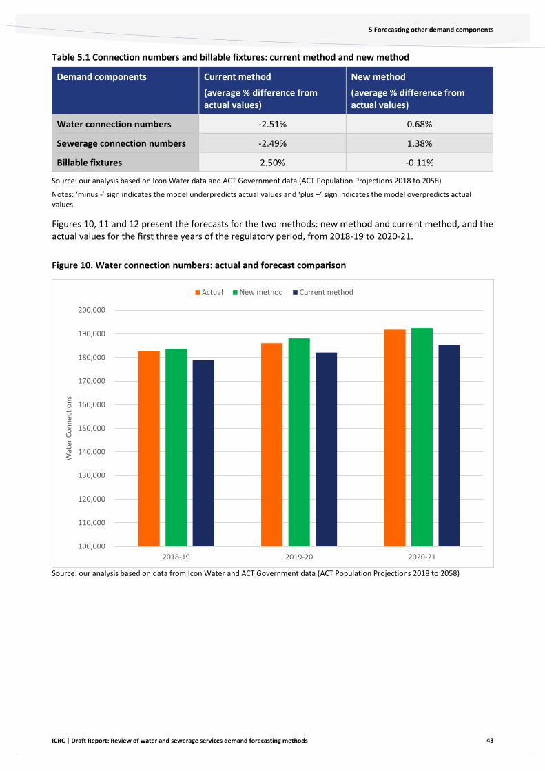
43
5 Forecasting other demand components
ICRC | Draft Report: Review of water and sewerage services demand forecasting methods
Table 5.1 Connection numbers and billable fixtures: current method and new method
Demand components Current method
(average % difference from actual values)
New method
(average % difference from actual values)
Water connection numbers -2.51% 0.68%
Sewerage connection numbers -2.49% 1.38%
Billable fixtures 2.50% -0.11%
Source: our analysis based on Icon Water data and ACT Government data (ACT Population Projections 2018 to 2058)
Notes: ‘minus -’ sign indicates the model underpredicts actual values and ‘plus +’ sign indicates the model overpredicts actual values.
Figures 10, 11 and 12 present the forecasts for the two methods: new method and current method, and the actual values for the first three years of the regulatory period, from 2018-19 to 2020-21.
Figure 10. Water connection numbers: actual and forecast comparison
Source: our analysis based on data from Icon Water and ACT Government data (ACT Population Projections 2018 to 2058)
100,000
110,000
120,000
130,000
140,000
150,000
160,000
170,000
180,000
190,000
200,000
2018-19 2019-20 2020-21
Wat
er C
on
nec
tio
ns
Actual New method Current method

44
5 Forecasting other demand components
ICRC | Draft Report: Review of water and sewerage services demand forecasting methods
Figure 11. Sewerage connection numbers: actuals and forecast comparison
Source: our analysis based on data from Icon Water and ACT Government data (ACT Population Projections 2018 to 2058)
100,000
110,000
120,000
130,000
140,000
150,000
160,000
170,000
180,000
190,000
200,000
2018-19 2019-20 2020-21
Sew
erag
e C
on
nec
tio
ns
Actual New method Current method
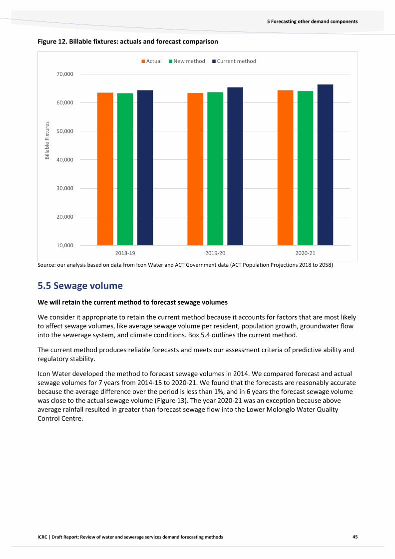
45
5 Forecasting other demand components
ICRC | Draft Report: Review of water and sewerage services demand forecasting methods
Figure 12. Billable fixtures: actuals and forecast comparison
Source: our analysis based on data from Icon Water and ACT Government data (ACT Population Projections 2018 to 2058)
5.5 Sewage volume
We will retain the current method to forecast sewage volumes
We consider it appropriate to retain the current method because it accounts for factors that are most likely to affect sewage volumes, like average sewage volume per resident, population growth, groundwater flow into the sewerage system, and climate conditions. Box 5.4 outlines the current method.
The current method produces reliable forecasts and meets our assessment criteria of predictive ability and regulatory stability.
Icon Water developed the method to forecast sewage volumes in 2014. We compared forecast and actual sewage volumes for 7 years from 2014-15 to 2020-21. We found that the forecasts are reasonably accurate because the average difference over the period is less than 1%, and in 6 years the forecast sewage volume was close to the actual sewage volume (Figure 13). The year 2020-21 was an exception because above average rainfall resulted in greater than forecast sewage flow into the Lower Molonglo Water Quality Control Centre.
10,000
20,000
30,000
40,000
50,000
60,000
70,000
2018-19 2019-20 2020-21
Bill
able
Fix
ture
s
Actual New method Current method
46
5 Forecasting other demand components
ICRC | Draft Report: Review of water and sewerage services demand forecasting methods
Figure 13. Sewage volume: actuals and forecast comparison
Source: our analysis based on Icon Water data
Icon Water supports the current method
Icon Water considers the current approach to forecast sewage volume is performing well and did not propose any changes (Icon Water 2021).
Box 5.4 Method to forecast sewage volumes
Icon Water uses historical average sewage flow into the Lower Molonglo Water Quality Control Centre from 1998 to 2013, and estimates the long-term trend in sewage volume for four scenarios that are based on assumptions about:
• average annual sewage volume per resident which depends on water conservation practices
• population projections
• long term weather scenarios (dry, average or wet)
• seasonal impact
• rates of groundwater or surface storm water flow into the sewerage system
The average of the four scenario is used to forecast sewage volumes.
0
5
10
15
20
25
30
35
40
45
2014-15 2015-16 2016-17 2017-18 2018-19 2019-20 2020-21
Sew
era
ge V
olu
me
s (G
L/Ye
ar)
FORECAST
ACTUAL
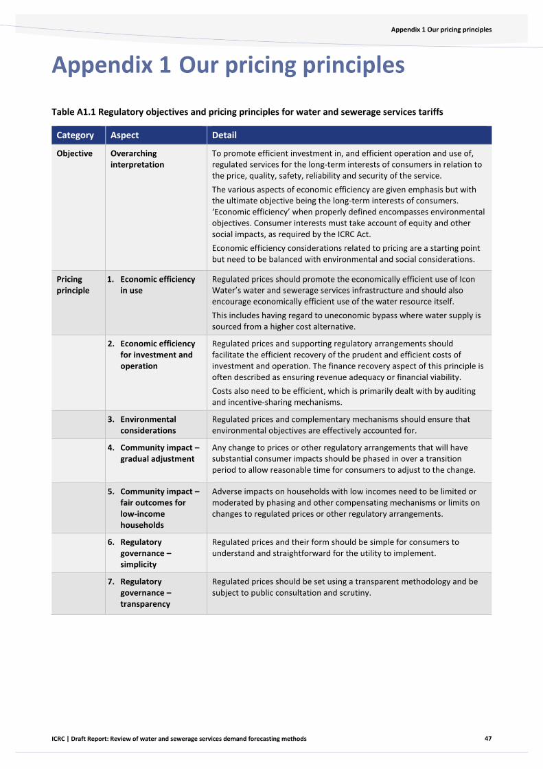
47
Appendix 1 Our pricing principles
ICRC | Draft Report: Review of water and sewerage services demand forecasting methods
Appendix 1 Our pricing principles
Table A1.1 Regulatory objectives and pricing principles for water and sewerage services tariffs
Category Aspect Detail
Objective Overarching interpretation
To promote efficient investment in, and efficient operation and use of, regulated services for the long-term interests of consumers in relation to the price, quality, safety, reliability and security of the service.
The various aspects of economic efficiency are given emphasis but with the ultimate objective being the long-term interests of consumers. ‘Economic efficiency’ when properly defined encompasses environmental objectives. Consumer interests must take account of equity and other social impacts, as required by the ICRC Act.
Economic efficiency considerations related to pricing are a starting point but need to be balanced with environmental and social considerations.
Pricing principle
1. Economic efficiency in use
Regulated prices should promote the economically efficient use of Icon Water’s water and sewerage services infrastructure and should also encourage economically efficient use of the water resource itself.
This includes having regard to uneconomic bypass where water supply is sourced from a higher cost alternative.
2. Economic efficiency for investment and operation
Regulated prices and supporting regulatory arrangements should facilitate the efficient recovery of the prudent and efficient costs of investment and operation. The finance recovery aspect of this principle is often described as ensuring revenue adequacy or financial viability.
Costs also need to be efficient, which is primarily dealt with by auditing and incentive-sharing mechanisms.
3. Environmental considerations
Regulated prices and complementary mechanisms should ensure that environmental objectives are effectively accounted for.
4. Community impact – gradual adjustment
Any change to prices or other regulatory arrangements that will have substantial consumer impacts should be phased in over a transition period to allow reasonable time for consumers to adjust to the change.
5. Community impact – fair outcomes for low-income households
Adverse impacts on households with low incomes need to be limited or moderated by phasing and other compensating mechanisms or limits on changes to regulated prices or other regulatory arrangements.
6. Regulatory governance – simplicity
Regulated prices and their form should be simple for consumers to understand and straightforward for the utility to implement.
7. Regulatory governance – transparency
Regulated prices should be set using a transparent methodology and be subject to public consultation and scrutiny.

48
Appendix 2 Technical details of the draft decision form of forecasting model for dam abstractions
ICRC | Draft Report: Review of water and sewerage services demand forecasting methods
Appendix 2 Technical details of the draft decision form of forecasting model for dam abstractions
Form of the ARIMA model Table A2.1 Regulatory objectives and pricing principles for water and sewerage services tariffs
Variable Description Reasoning Coefficient estimate from modelling exercise
Dam abstractions Dam abstractions during a previous week
Dam abstractions are related over time. This is a function of the ARIMA model and is calculated using the model.
0.68
Data shows dam abstractions are positively
related over time.
Temperature Average of daily
maximum
temperatures
(degrees Celsius)
during a week
Hot periods will
result in more water
abstractions to meet
increasing water
demand by
customers
Linear component: 3.70 to 7.73
Squared: 0.05
These estimates show that dam abstractions
increase in hot periods, and the squared
component show that the increase in
abstractions is more than proportionately to
the increase in temperature.
Rainfall Average daily
rainfall (mm) during
a week
Rainy periods will
result in less water
abstractions because
part of customer’s
water demand will
be met by rain (e.g.
less water required
for plants during
rainy periods)
Non-linear components
• Squared: 0.38
• Square root: -25.30 to -13.32
These estimates together show a negative
relationship between total abstractions and
rainfall.
Evaporation Average daily
evaporation during
a week
High evaporation
rates will result in
more water
abstractions to meet
higher irrigation
requirements for
plants/gardens as
they dry.
Linear component: 25.10 to 101.40
Squared: -6.40
Square root: -202.92
These estimates together show that total
abstractions increase with higher levels of
evaporation, and the non-linear components
show that abstractions increase less than
proportionately.
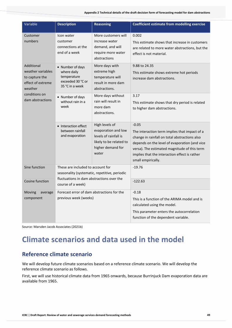
49
Appendix 2 Technical details of the draft decision form of forecasting model for dam abstractions
ICRC | Draft Report: Review of water and sewerage services demand forecasting methods
Variable Description Reasoning Coefficient estimate from modelling exercise
Customer
numbers
Icon water
customer
connections at the
end of a week
More customers will
increase water
demand, and will
require more water
abstractions
0.002
This estimate shows that increase in customers
are related to more water abstractions, but the
effect is not material.
Additional
weather variables
to capture the
effect of extreme
weather
conditions on
dam abstractions
• Number of days where daily temperature exceeded 30 °C or 35 °C in a week
More days with
extreme high
temperature will
result in more dam
abstractions.
9.88 to 24.35
This estimate shows extreme hot periods
increase dam abstractions.
• Number of days without rain in a week
More days without
rain will result in
more dam
abstractions.
3.17
This estimate shows that dry period is related
to higher dam abstractions.
• Interaction effect between rainfall and evaporation
High levels of
evaporation and low
levels of rainfall is
likely to be related to
higher demand for
water
-0.05
The interaction term implies that impact of a
change in rainfall on total abstractions also
depends on the level of evaporation (and vice
versa). The estimated magnitude of this term
implies that the interaction effect is rather
small empirically.
Sine function These are included to account for
seasonality (systematic, repetitive, periodic
fluctuations in dam abstractions over the
course of a week)
-19.76
Cosine function -122.63
Moving average
component
Forecast error of dam abstractions for the
previous week (weeks)
-0.18
This is a function of the ARIMA model and is
calculated using the model.
This parameter enters the autocorrelation
function of the dependent variable.
Source: Marsden Jacob Associates (2021b)
Climate scenarios and data used in the model
Reference climate scenario
We will develop future climate scenarios based on a reference climate scenario. We will develop the reference climate scenario as follows.
First, we will use historical climate data from 1965 onwards, because Burrinjuck Dam evaporation data are available from 1965.

50
Appendix 2 Technical details of the draft decision form of forecasting model for dam abstractions
ICRC | Draft Report: Review of water and sewerage services demand forecasting methods
Second, for this draft decision we assume historical data are available till December 2021. The time period between July 1965 and December 2021 will be divided into 50 overlapping 6.5-year time periods.7 We have chosen 6.5 years as the length of each period because if we do the forecast in early 2022 which is around 1.5 years before the start of the five-year regulatory period of July 2023.
Third, we will develop reference climate scenario using the average data for the 50 time periods. That means our reference climate scenario has daily data for the maximum temperature, rainfall and evaporation for a 6.5-year time period.
Proposed approach to future climate scenarios using NARCLiM
NARCLiM projections include the latest set of global climate models (GCMs) provided by the Intergovernmental Panel on Climate Change. Each GCM (there are 3) consists of 2 separate Regional Climate Models (RCMs), which in turn provides projections based on two emissions scenarios, referred to as Representation Concentration Pathways (RCPs):8
• RCP4.5 – A scenario which assumes some mitigation of greenhouse gas emissions is achieved
• RCP8.5 – A scenario which assumes very limited mitigation of greenhouse gas emissions is achieved
NARCLiM provides data on 12 different climate scenarios, made up of the different combinations of GCMs (3), RCMs (2) and RCPs (2).
NARCLiM provides projections by observing trends in historical data from 1951 to 2005.
In our demand forecasting model, we will use the rainfall, evaporation and temperature variables to develop our future climate scenarios.
Approach to developing adjustment factors
Each NARCLiM scenario gives the average monthly rainfall, temperature and evaporation projections from 2020 to 2100.
We propose to use the following steps to determine the adjustment factors:
1. Monthly historical data from 1951 to 2005 is provided by the NARCLiM data source for temperature, rainfall and evaporation. Average monthly values are created for this 55-year period and then grouped to determine seasonal averages for the period.
2. We will use monthly projections from 2022 to 2028 to coincide with the forecast period. Using the same process as step 1, seasonal averages are determined for the period.
3. Adjustment factors are calculated as the percentage change between the seasonal values for the 2022-2028 period and the 1951-2005 period for rainfall and evaporation, while the adjustment factor for temperature is taken as the difference.
We will finalise the above steps in our final report.
Forecast of water installation numbers
We need forecasts of water installation numbers to forecast dam abstractions. We will use ACT population projections to forecast water installation numbers, as discussed in section 5.4 of this report.
—————
7 Overlapping periods are determined by subtracting the overlap period from the number of years of data observations. For example, there are 57 yearly observations between 1965 and 2022, subtracting the 5.5-year overlap period from this gives 51.5 overlapping periods, which we have rounded down to 51 periods.
8 Climate Data Portal (nsw.gov.au)
51
Appendix 2 Technical details of the draft decision form of forecasting model for dam abstractions
ICRC | Draft Report: Review of water and sewerage services demand forecasting methods
Data used in the model
Dam abstractions
This is the variable we forecast using the model. Icon Water abstractions water from its dams to meet demand from ACT and Queanbeyan customers. This data is sourced from Icon Water.
Maximum temperature
Temperature data will be sourced from the Bureau of Meteorology, which reports weather data for Canberra based on the weather conditions at Canberra Airport weather station. Temperature data is used in the model because water demand changes with temperature, with hot days having more demand.
Rainfall
Rainfall data at Canberra Airport will be sourced from the Bureau of Meteorology. Rainfall data is used because water demand changes with the amount of rainfall, with rainy days having less demand for water.
Evaporation
Evaporation data for Burrinjuck Dam, measured in millimetres, will be sources from the Bureau of Meteorology. The Bureau of Meteorology measures evaporation as the amount of water which evaporates from a specific standardized open space. The model uses data for Burrinjuck Dam because historical data for Canberra Airport weather station (like for other climate variables) is not available for a longer time period.
December dummy variable
The model has a dummy variable for December to capture the effect of that month on water demand. Water demand in December is higher than other months in the ACT, likely due to high temperatures and summer holidays.
Summer dummy variables
The model has a dummy variable for summer season (December to February) to capture the effect of hot summer season on water demand.
Water customer numbers
The model has the number of Icon Water’s water customers, as measured by the number of water connections. Water customer numbers have been included because there is a strong positive correlation between customer numbers and water demand. Data for actual customer numbers is provided by Icon Water.
A Fourier seasonal term
Adding a Fourier seasonal term to a forecasting model is a statistical technique used to incorporate annual regular and predictable changes in water demand to the forecasting model. Accuracy of forecasts can be improved by incorporating regular and predictable changes to the model. Data for a Fourier term is created using a mathematical formula.

52
Appendix 3 Technical details of the draft decision forecasting model for other demand components
ICRC | Draft Report: Review of water and sewerage services demand forecasting methods
Appendix 3 Technical details of the draft decision forecasting model for other demand components
Total ACT water sales Figure 14 shows the relationship between annual dam abstractions and billed consumption from 1999-2000 to 2020-21. As seen in the figure, there is a strong relationship between the two variables.
Figure 14 Annual dam abstractions and billed consumption, 1999-2000 to 2020-21
Source: our analysis based on data from Icon Water
Billed water sales at Tier 1 and Tier 2
Tier 1 proportion
To estimate the proportion of total water sales that is expected to fall into the Tier 1 category, we estimate an equation that best fits the relationship between the average amount of water consumed per connection and proportion of total sales falling into the Tier 1 category.
We have re-estimated different forms of the relationship using the latest available data to date and identified that our current equation still provides the best fit. Table A3.1 shows the relationship between
y = 0.8336x + 416.85R² = 0.9621
30,000.00
35,000.00
40,000.00
45,000.00
50,000.00
55,000.00
60,000.00
30,000.00 35,000.00 40,000.00 45,000.00 50,000.00 55,000.00 60,000.00 65,000.00 70,000.00
Co
nsu
mp
tio
n (
ML)
Abstraction (ML)

53
Appendix 3 Technical details of the draft decision forecasting model for other demand components
ICRC | Draft Report: Review of water and sewerage services demand forecasting methods
the average amount of water consumed per connection and observed Tier 1 proportion from 2008-09 to 2020-21.
Table A3.1 Observed sales by Tier and connection numbers
Year Total ACT sales (ML)
Tier 1 sales (ML)
Tier 2 sales (ML)
Connections (#)
ML/ connection/
year
Observed
Tier 1 proportion
2008–09 38,179 20,448 17,731 144,165 0.265 53.56
2009–10 37,744 21,485 16,259 146,853 0.257 56.92
2010–11 33,780 20,906 12,874 149,794 0.226 61.89
2011–12 35,393 21,851 13,541 153,256 0.231 61.74
2012–13 40,428 23,032 17,396 158,258 0.255 56.97
2013–14 41,928 23,759 18,169 163,223 0.257 56.67
2014–15 39,152 23,652 15,500 166,886 0.235 60.41
2015–16 41,786 24,393 17,393 168,981 0.247 58.38
2016-17 41,182 24,650 16,532 173,715 0.237 59.86
2017-18 42,581 25,019 17,562 178,728 0.238 58.76
2018-19 41,808 26,324 15,484 182,599 0.229 62.96
2019-20 45,795 27,059 18,736 185,997 0.246 59.09
2020-21 41,472 26,130 15,343 191,803 0.216 63.00
Source: our analysis based on data from Icon Water
Figure 15 shows the observed relationship between the Tier 1 proportion and average customer consumption. A visual examination of the data suggests an exponential relationship.
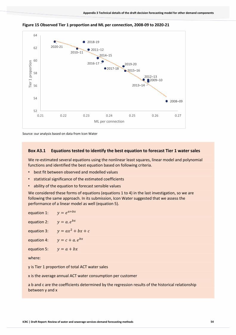
54
Appendix 3 Technical details of the draft decision forecasting model for other demand components
ICRC | Draft Report: Review of water and sewerage services demand forecasting methods
Figure 15 Observed Tier 1 proportion and ML per connection, 2008-09 to 2020-21
Source: our analysis based on data from Icon Water
Box A3.1 Equations tested to identify the best equation to forecast Tier 1 water sales
We re-estimated several equations using the nonlinear least squares, linear model and polynomial functions and identified the best equation based on following criteria.
• best fit between observed and modelled values
• statistical significance of the estimated coefficients
• ability of the equation to forecast sensible values
We considered these forms of equations (equations 1 to 4) in the last investigation, so we are following the same approach. In its submission, Icon Water suggested that we assess the performance of a linear model as well (equation 5).
equation 1: 𝑦 = 𝑒𝑎+𝑏𝑥
equation 2: 𝑦 = 𝑎. 𝑒𝑏𝑥
equation 3: 𝑦 = 𝑎𝑥2 + 𝑏𝑥 + 𝑐
equation 4: 𝑦 = 𝑐 + 𝑎. 𝑒𝑏𝑥
equation 5: 𝑦 = 𝑎 + 𝑏𝑥
where:
y is Tier 1 proportion of total ACT water sales
x is the average annual ACT water consumption per customer
a b and c are the coefficients determined by the regression results of the historical relationship between y and x
2008–09
2009–10
2010–11 2011–12
2012–13
2013–14
2014–15
2015–16
2016-17
2017-18
2018-19
2019-20
2020-21
52
54
56
58
60
62
64
0.21 0.22 0.23 0.24 0.25 0.26 0.27
Tier
1 p
rop
ort
ion
ML per connection
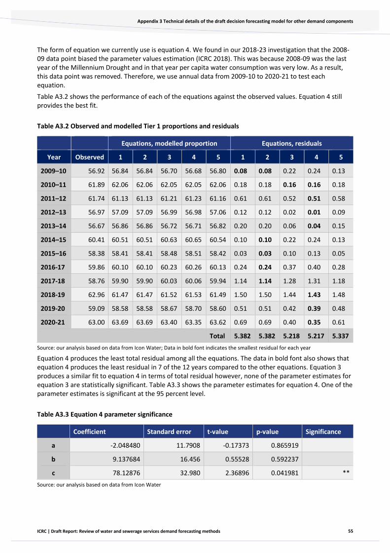
55
Appendix 3 Technical details of the draft decision forecasting model for other demand components
ICRC | Draft Report: Review of water and sewerage services demand forecasting methods
The form of equation we currently use is equation 4. We found in our 2018-23 investigation that the 2008-09 data point biased the parameter values estimation (ICRC 2018). This was because 2008-09 was the last year of the Millennium Drought and in that year per capita water consumption was very low. As a result, this data point was removed. Therefore, we use annual data from 2009-10 to 2020-21 to test each equation.
Table A3.2 shows the performance of each of the equations against the observed values. Equation 4 still provides the best fit.
Table A3.2 Observed and modelled Tier 1 proportions and residuals
Equations, modelled proportion Equations, residuals
Year Observed 1 2 3 4 5 1 2 3 4 5
2009–10 56.92 56.84 56.84 56.70 56.68 56.80 0.08 0.08 0.22 0.24 0.13
2010–11 61.89 62.06 62.06 62.05 62.05 62.06 0.18 0.18 0.16 0.16 0.18
2011–12 61.74 61.13 61.13 61.21 61.23 61.16 0.61 0.61 0.52 0.51 0.58
2012–13 56.97 57.09 57.09 56.99 56.98 57.06 0.12 0.12 0.02 0.01 0.09
2013–14 56.67 56.86 56.86 56.72 56.71 56.82 0.20 0.20 0.06 0.04 0.15
2014–15 60.41 60.51 60.51 60.63 60.65 60.54 0.10 0.10 0.22 0.24 0.13
2015–16 58.38 58.41 58.41 58.48 58.51 58.42 0.03 0.03 0.10 0.13 0.05
2016-17 59.86 60.10 60.10 60.23 60.26 60.13 0.24 0.24 0.37 0.40 0.28
2017-18 58.76 59.90 59.90 60.03 60.06 59.94 1.14 1.14 1.28 1.31 1.18
2018-19 62.96 61.47 61.47 61.52 61.53 61.49 1.50 1.50 1.44 1.43 1.48
2019-20 59.09 58.58 58.58 58.67 58.70 58.60 0.51 0.51 0.42 0.39 0.48
2020-21 63.00 63.69 63.69 63.40 63.35 63.62 0.69 0.69 0.40 0.35 0.61
Total 5.382 5.382 5.218 5.217 5.337
Source: our analysis based on data from Icon Water; Data in bold font indicates the smallest residual for each year
Equation 4 produces the least total residual among all the equations. The data in bold font also shows that equation 4 produces the least residual in 7 of the 12 years compared to the other equations. Equation 3 produces a similar fit to equation 4 in terms of total residual however, none of the parameter estimates for equation 3 are statistically significant. Table A3.3 shows the parameter estimates for equation 4. One of the parameter estimates is significant at the 95 percent level.
Table A3.3 Equation 4 parameter significance
Coefficient Standard error t-value p-value Significance
a -2.048480 11.7908 -0.17373 0.865919
b 9.137684 16.456 0.55528 0.592237
c 78.12876 32.980 2.36896 0.041981 **
Source: our analysis based on data from Icon Water

56
Appendix 3 Technical details of the draft decision forecasting model for other demand components
ICRC | Draft Report: Review of water and sewerage services demand forecasting methods
Figure 16 shows the modelled Tier 1 proportion over the 2009-10 to 2020-21 period, in comparison to the observed values.
Figure 16 Observed and modelled Tier 1 proportion
Source: our analysis based on data from Icon Water
Water connections, sewerage connections and billable fixtures We will be changing the approach we use to forecast water and sewerage connection numbers and billable fixtures. We will be using the ACT Government population projections to forecast these variables. As noted in section 4.2 of this draft report, the ACT Government’s population projections are currently being updated to account for the effect of Covid-19, and the updated projections are expected to be published in the second half of 2021. We will monitor this development to ensure that the ACT population projections we use account for the impact of the pandemic
We tested this approach for the current regulatory period and obtained forecasts from 2018-19 to 2020-21 and then compared them to the actual values for the same period.
We first estimated the historical relationship between ACT population9 and each of the three variables: water connection numbers, sewerage connection numbers and billable fixtures.
We modelled each relationship using a linear regression model.
—————
9 Data source used for historical population data: National, state and territory population, December 2020 | Australian Bureau of Statistics (abs.gov.au)
50
52
54
56
58
60
62
64
0.21 0.215 0.22 0.225 0.23 0.235 0.24 0.245 0.25 0.255 0.26
Tier
1 p
rop
ort
ion
ML per connection
Observed Modelled

57
Appendix 3 Technical details of the draft decision forecasting model for other demand components
ICRC | Draft Report: Review of water and sewerage services demand forecasting methods
To estimate the historical relationship between water connection numbers and ACT Population, we used annual ACT Population data and water connection numbers from 2008-09 to 2017-18. Year 2008-09 was used because this is the oldest date for which we have data. We then ran a linear regression model. Figure 17 shows the result of the regression. For the next regulatory period, we will re-estimate this relationship using the latest data available to date.
Figure 17 Relationship between ACT population and water connection numbers (2008-09 to 2017-18)
Source: our analysis based on data from Icon Water and ABS ACT Population data (ABS National, state and territory population)
To estimate the historical relationship between sewerage connection numbers and ACT Population, we used annual ACT Population data and sewerage connection numbers from 2012-13 to 2017-18. Year 2012-13 was used because this is the oldest date for which we had data. We then ran a linear regression model. Figure 18 shows the result of the regression. For the next regulatory period, we will re-estimate this relationship using the latest data available to date.
y = 0.5459x - 50266R² = 0.9909
100,000
110,000
120,000
130,000
140,000
150,000
160,000
170,000
180,000
190,000
350000 360000 370000 380000 390000 400000 410000 420000 430000
Wat
er c
on
nec
tio
n n
um
ber
s
ACT Population
Water connection numbers
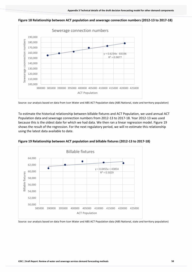
58
Appendix 3 Technical details of the draft decision forecasting model for other demand components
ICRC | Draft Report: Review of water and sewerage services demand forecasting methods
Figure 18 Relationship between ACT population and sewerage connection numbers (2012-13 to 2017-18)
Source: our analysis based on data from Icon Water and ABS ACT Population data (ABS National, state and territory population)
To estimate the historical relationship between billable fixtures and ACT Population, we used annual ACT Population data and sewerage connection numbers from 2012-13 to 2017-18. Year 2012-13 was used because this is the oldest date for which we had data. We then ran a linear regression model. Figure 19 shows the result of the regression. For the next regulatory period, we will re-estimate this relationship using the latest data available to date.
Figure 19 Relationship between ACT population and billable fixtures (2012-13 to 2017-18)
Source: our analysis based on data from Icon Water and ABS ACT Population data (ABS National, state and territory population)
y = 0.6234x - 83336R² = 0.9877
100,000
110,000
120,000
130,000
140,000
150,000
160,000
170,000
180,000
190,000
380000 385000 390000 395000 400000 405000 410000 415000 420000 425000
Sew
eara
ge c
oo
nn
ecti
on
nu
mb
ers
ACT Population
Sewerage connection numbers
y = 0.0455x + 43854R² = 0.5029
50,000
52,000
54,000
56,000
58,000
60,000
62,000
64,000
385000 390000 395000 400000 405000 410000 415000 420000 425000
Bill
able
fix
ture
s
ACT Population
Billable fixtures
59
Appendix 3 Technical details of the draft decision forecasting model for other demand components
ICRC | Draft Report: Review of water and sewerage services demand forecasting methods
We applied each of these regressions to ACT Government population projections10 data from 2018-19 to 2020-21 to forecast water connections, sewerage connection and billable fixtures for the same period.
We compared these forecasts to actual values of connection numbers and billable fixtures from 2018-19 to 2020-21 to assess forecast accuracy. Table A3.4 shows this comparison.
Table A3.4 Connection numbers and billable fixtures: forecast and actuals
Year Water connections numbers
Sewerage connection numbers
Billable fixtures
Forecast Actual Forecast Actual Forecast Actual
2018-19 183,657 182,599 183,797 182,221 63,351 63,554
2019-20 188,093 185,997 188,862 185,586 63,721 63,440
2020-21 192,469 191,803 193,859 191,013 64,086 64,367
Source: our analysis based on data from Icon Water and ACT Government data (ACT Population Projections 2018 to 2058)
—————
10 Data source for ACT Populations Projections: ACT Population Projection: 2018 to 2058
60
ICRC | Draft Report: Review of water and sewerage services demand forecasting methods
Appendix 4 Consultant’s stage 2 report
Water demand forecasting methodology review – Stage 2 Draft report
15 September 2021
A Marsden Jacob Report

61
Appendix 4 Consultant’s stage 2 report
ICRC | Draft Report: Review of water and sewerage services demand forecasting methods
Prepared or Independent Competition and Regulatory Commission
Marsden Jacob Associates Pty Ltd
ABN 66 663 324 657
ACN 072 233 204
t. 03 8808 7400
Office locations
Melbourne
Perth
Sydney
Brisbane
Adelaide
Authors
Rob Nolan Associate Director
Prof Vasilis Sarafidis Senior Associate
Dr Jeremy Cheesman Director
LinkedIn - Marsden Jacob Associates
www.marsdenjacob.com.au
Acknowledgements
Marsden Jacob consulted widely for this report. We would like to acknowledge and thank all the people we engaged with during this project. The
report is better for your input. All final recommendations and views in this report are attributable to Marsden Jacob unless otherwise stated.
Statement of Confidentiality
The contents of this report and any attachments are confidential and are intended solely for the addressee. The information may also be legally
privileged. If you have received this report in error, any use, reproduction or dissemination is strictly prohibited. If you are not the intended
recipient, please immediately notify the sender by reply e-mail or phone and delete this report and its attachments, if any.
Disclaimer
This document has been prepared in accordance with the scope of services described in the contract or agreement between Marsden Jacob
Associates Pty Ltd ACN 072 233 204 (Marsden Jacob) and the Client. This document is supplied in good faith and reflects the knowledge,
expertise and experience of the advisors involved. The document and findings are subject to assumptions and limitations referred to within the
document. Any findings, conclusions or recommendations only apply to the aforementioned circumstances and no greater reliance should be
assumed or drawn by the Client. Marsden Jacob accepts no responsibility whatsoever for any loss occasioned by any person acting or refraining
from action because of reliance on the document. The document has been prepared solely for use by the Client and Marsden Jacob Associates
accepts no responsibility for its use by other parties.

62
Appendix 4 Consultant’s stage 2 report
ICRC | Draft Report: Review of water and sewerage services demand forecasting methods
Executive summary 64
This report 64
1. Introduction 69
1.1 Objectives 69
1.2 Approach and report structure 70
2. Model specification and approach to updating ARIMA. 72
2.1 Updating model specification 72
2.2 Steps to ensure model and parameters are statistically sound 74
2.3 Implementation of model changes 75
3. Assessment on the current ARIMA approach 76
3.1 Time frequency (Short-term versus long-term forecasts using daily data) 76
3.2 Ability to model extreme weather scenarios 79
3.3 Future climatic scenarios 80
3.4 Population projections 81
3.5 Forecasting accuracy 82
3.6 Model uncertainty vs uncertainty in predicting weather conditions. 82
3.7 Estimation and lag order selection 83
3.8 Policy adjustments 83
3.9 Terminology 83
4. Modelling exercise 84
4.1 Approach 84
4.2 Explanatory variables for weather conditions 85
4.3 ARIMAX model with lower frequency data 86
4.4 Results 86
Appendix 1. ARIMA model assessment – detailed analysis 89
A1.1. Short-term versus long-term forecast using daily data 89
A1.2. Detailed results of the modelling exercise done in stage 2 review 92
A1.3. Stata model estimate outcome: weekly observations 95
A1.4. Stata model estimate outcome: monthly observations 96
A1.5. Stata model estimate outcome: daily observations 97
63
Appendix 4 Consultant’s stage 2 report
ICRC | Draft Report: Review of water and sewerage services demand forecasting methods
Tables
Table 5: Stage 2 modelling exercise: variables used for weekly data model 65
Table 6: Updated model variables for the weekly form of the model and data source 73
Table 7: Forecast value of yearly total demand 79
Table 8 Population projections ACT under pre and post COVID scenarios 81
Table 9: Forecasting accuracy using daily, weekly and monthly data 87
Table 10: Form of variables used in daily, weekly and monthly data models 92
Table 11: Coefficient estimates for current ICRC ARIMA model and models used in the modelling exercise with daily, weekly and monthly observations 92
Figures
Figure 20: ICRC review approach 69
Figure 21: Report structure 71
Figure 22: Actual vs forecast volumes using daily data, July 2018 – June 2021 88
Figure 23: Actual vs forecast volumes using weekly data, July 2018 – June 2021 88
Figure 24: Actual vs forecast volumes using monthly data, July 2018 – June 2021 89
Figure 25: Variable of forecast error as the forecasting horizon increases 91
64
Appendix 4 Consultant’s stage 2 report
ICRC | Draft Report: Review of water and sewerage services demand forecasting methods
Executive summary
Marsden Jacob Associates has been engaged to review Icon Water’s demand
forecasting methodology in preparation for the Independent Competition and
Regulatory Commission’s 2023 price review.
Our advice to the ICRC covers two stages, with objectives set out below.
Stage 1
In Stage 1, the ICRC asked us to advise on whether the current Auto-Regressive Integrated Moving Average (ARIMA) approach to forecasting water demand is appropriate and fit for purpose, considering other approaches that could be used. The ICRC also asked us to advise on whether there would be significant benefits from moving to an alternative forecasting approach.
Our Stage 1 advice supported the use of the ARIMA model and is available on the ICRC website here.
Stage 2
In the second stage, the ICRC asked us to advise on how to best implement the forecasting approach that the ICRC chooses, following our Stage 1 advice. ICRC has asked our advice the address matters including:
• the general model specification, including dependent and explanatory variables and functional form
• how to ensure the model can appropriately account for changes in climate and demographics (e.g., population
projections)
• any steps needed to ensure the model and parameters are statistically sound (e.g. parameters are stationary
and structural breaks in time series are dealt with appropriately)
• how recommended changes should be made/implemented, including advising on the data sources and any
adjustments that would be needed (e.g. adjustments to make data stationary).
This report This report is our final deliverable for Stage 2. Our Stage 2 report outlines the updated water demand forecasting
model specification and recommended approach to updating the ARIMA model for the next regulatory period.
The model specification and recommended approach for updating the ARIMA model set out in this report will be implemented in Stage 3 of the ICRC model review. We note that model implementation, testing and refinement during Stage 3 may result in the final demand model specification and parameters values being different from those included in this report. Material in this section should be read with this in mind. Initial estimates in this report have been provided at the request of the ICRC, and to give stakeholders an understanding of the order of magnitude of the coefficients for model parameters estimated to date, where data has been available.
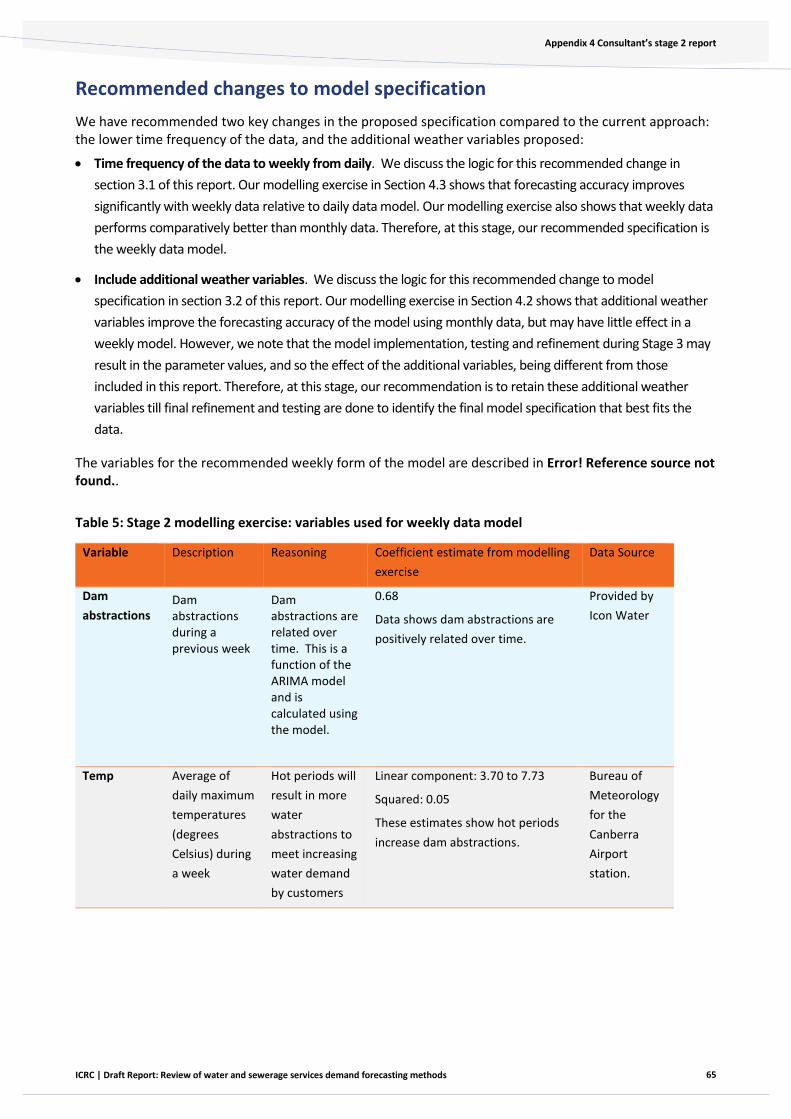
65
Appendix 4 Consultant’s stage 2 report
ICRC | Draft Report: Review of water and sewerage services demand forecasting methods
Recommended changes to model specification
We have recommended two key changes in the proposed specification compared to the current approach: the lower time frequency of the data, and the additional weather variables proposed:
• Time frequency of the data to weekly from daily. We discuss the logic for this recommended change in
section 3.1 of this report. Our modelling exercise in Section 4.3 shows that forecasting accuracy improves
significantly with weekly data relative to daily data model. Our modelling exercise also shows that weekly data
performs comparatively better than monthly data. Therefore, at this stage, our recommended specification is
the weekly data model.
• Include additional weather variables. We discuss the logic for this recommended change to model
specification in section 3.2 of this report. Our modelling exercise in Section 4.2 shows that additional weather
variables improve the forecasting accuracy of the model using monthly data, but may have little effect in a
weekly model. However, we note that the model implementation, testing and refinement during Stage 3 may
result in the parameter values, and so the effect of the additional variables, being different from those
included in this report. Therefore, at this stage, our recommendation is to retain these additional weather
variables till final refinement and testing are done to identify the final model specification that best fits the
data.
The variables for the recommended weekly form of the model are described in Error! Reference source not found..
Table 5: Stage 2 modelling exercise: variables used for weekly data model
Variable Description Reasoning Coefficient estimate from modelling
exercise
Data Source
Dam
abstractions Dam abstractions during a previous week
Dam abstractions are related over time. This is a function of the ARIMA model and is calculated using the model.
0.68
Data shows dam abstractions are
positively related over time.
Provided by
Icon Water
Temp Average of
daily maximum
temperatures
(degrees
Celsius) during
a week
Hot periods will
result in more
water
abstractions to
meet increasing
water demand
by customers
Linear component: 3.70 to 7.73
Squared: 0.05
These estimates show hot periods
increase dam abstractions.
Bureau of
Meteorology
for the
Canberra
Airport
station.

66
Appendix 4 Consultant’s stage 2 report
ICRC | Draft Report: Review of water and sewerage services demand forecasting methods
Variable Description Reasoning Coefficient estimate from modelling
exercise
Data Source
rain Average daily
rainfall (mm)
during a week
Rainy periods
will result in less
water
abstractions
because part of
customer’s
water demand
will be met by
rain (e.g. less
water required
for plants
during rainy
periods)
Squared: 0.38
Square root: -25.30 to -13.32
These estimates combined show a
negative relationship between total
abstractions and rainfall.
Evap Average daily
evaporation
during a week
High
evaporation
rates will result
in more water
abstractions to
meet higher
irrigation
requirements
for
plants/gardens
as they dry.
Linear component: 25.10 to 101.40
Squared: -6.40
Square root: -202.92
These estimates combined show a
positive relationship between total
abstractions and evaporation
Bureau of
Meteorology
for the
Burrinjuck
Dam station
customer Icon water
customer
connections at
the end of a
week
More customers
will increase
water demand,
and will require
more water
abstractions
0.002
This estimate shows that increase in
customers are related to more water
abstractions, but the effect is not
material.
Provided by
Icon Water
Additional
weather
variables to
capture the
effect of
extreme
weather
conditions on
dam
abstractions
• Number of days where daily temperature exceeded 30 °C or 35 °C in a week
More days with
extreme high
temperature
will result in
more dam
abstractions.
9.88 to 24.35
This estimate shows extreme hot
periods increase dam abstractions.
Bureau of
Meteorology
for the
Canberra
Airport
station and
Bureau of
Meteorology
for the
Burrinjuck
Dam station
• Number of days without rain in a week
More days
without rain will
result in more
dam
abstractions.
3.17
This estimate shows that dry period
is related to higher dam
abstractions.
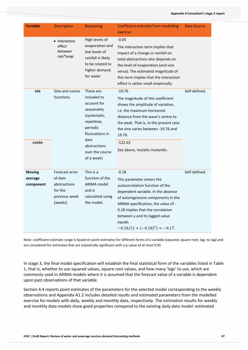
67
Appendix 4 Consultant’s stage 2 report
ICRC | Draft Report: Review of water and sewerage services demand forecasting methods
Variable Description Reasoning Coefficient estimate from modelling
exercise
Data Source
• Interaction effect between rain*evap
High levels of
evaporation and
low levels of
rainfall is likely
to be related to
higher demand
for water
-0.05
The interaction term implies that
impact of a change in rainfall on
total abstractions also depends on
the level of evaporation (and vice
versa). The estimated magnitude of
this term implies that the interaction
effect is rather small empirically.
𝐬𝐢𝐧 Sine and cosine
functions.
These are
included to
account for
seasonality
(systematic,
repetitive,
periodic
fluctuations in
dam
abstractions
over the course
of a week)
-19.76
The magnitude of this coefficient
shows the amplitude of variation,
i.e. the maximum horizontal
distance from the wave’s centre to
the peak. That is, in the present case
the sine varies between -19.76 and
19.76.
Self-defined
𝐜𝐨𝐬𝐢𝐧 -122.63
See above, mutatis mutandis.
Moving
average
component
Forecast error
of dam
abstractions
for the
previous week
(weeks)
This is a
function of the
ARIMA model
and is
calculated using
the model.
-0.18
This parameter enters the
autocorrelation function of the
dependent variable. In the absence
of autoregressive components in the
ARIMA specification, the value of -
0.18 implies that the correlation
between y and its lagged value
equals
−0.18 (1 + (−0.18)2) ≈ −0.17⁄ .
Self-defined
Note: coefficient estimate range is based on point estimates for different forms of a variable (squared, square root, lag, no lag) and
are considered for estimates that are statistically significant with a p-value of at most 0.05
In stage 3, the final model specification will establish the final statistical form of the variables listed in Table 1, that is, whether to use squared values, square root values, and how many ‘lags’ to use, which are commonly used in ARIMA models where it is assumed that the forecast value of a variable is dependent upon past observations of that variable.
Section 4.4 reports point estimates of the parameters for the selected model corresponding to the weekly observations and Appendix A1.2 includes detailed results and estimated parameters from the modelled exercise for models with daily, weekly and monthly data, respectively. The estimation results for weekly and monthly data models show good properties compared to the existing daily data model: estimated

68
Appendix 4 Consultant’s stage 2 report
ICRC | Draft Report: Review of water and sewerage services demand forecasting methods
coefficients have signs that are consistent with expectations; moreover, the new variables, which capture the effect of extreme weather conditions, improve the fit of the model.
As discussed in more detail in sections 3.1, 3.4, and 3.7 of this report, the recommended weekly data model specification better accounts for future changes in climate, demographics (e.g. population projections):
• Lower frequency data potentially avoid a clash between modelling climate change adaptation and
predictive ability over longer horizons, in that there is a plausible range of values for the autoregressive
parameter that is consistent with both.
• Computing forecasts of water installations based on ACT population projections produced by the
Australian Government’s Centre for Population has the advantage that these projections are up-to-date and
include the impact of Covid-19 and resulting border closures on future population growth. In contrast,
population (or water installation) projections based on past data, prior to 2020-21, do not consider the effect
of Covid-19, and therefore they are likely to be highly inaccurate. We understand the ICRC is considering
using the ACT Government’s population projections which accounts for future development activities in ACT
and is being updated to account for the effect of Covid-19.11
Steps to ensure model and parameters are statistically sound
There are several steps that will be implemented in Stage 3 to ensure the model and parameters are statistically sound, and to confirm the final model specification. We discuss these in section 3.2 of this report. These steps mainly deal with technical approaches that will be used for determining best model fit.
Implementation of model changes
We outline recommended steps for implementing model changes in section 2.3 of this report. This section details how the ARIMAX model should be implemented including the approach for developing in- and out-of-sample forecasts, testing of the time-step for the final model specification, and how to forecast future weather conditions. We recommend that future weather conditions are based on the NARCLiM database, a multi-agency research project between the NSW and ACT governments and the Climate Change Research Centre at the University of NSW.
—————
11 https://www.treasury.act.gov.au/snapshot/demography/act

69
Appendix 4 Consultant’s stage 2 report
ICRC | Draft Report: Review of water and sewerage services demand forecasting methods
1. Introduction
Marsden Jacob Associates has been engaged to review Icon Water’s demand
forecasting methodology in preparation for the Independent Competition and
Regulatory Commission’s 2023 price review.
The ICRC decided in its 2018 determination for water and sewerage services prices for Icon Water to review its demand forecasting model before the next price investigation.
The ICRC 2018 regulatory determination noted that the Auto-Regressive Integrated Moving Average (ARIMA) model for demand forecasting did not fully account for climate, demographic changes and projections. ICRC identified these issues as potential weaknesses in the forecasting model.
The ICRC determination also noted that the medium-term demand forecasts were highly sensitive to minor updates to the data used in the model. The ICRC has noted that this may reflect the weighting of recent observations and absence of leading indicators in the model. This has also been identified as a potential weakness in the forecasting model.
The ICRC review is being undertaken in consultation with key stakeholders. As part of this, ICRC released an issues paper in May 2021, held a workshop and sought submissions during June and July. ICRC will consult with stakeholders through submissions and workshops following release of the draft report (Figure 20). The final model specification from the next stage of this review will be used to produce forecasts for the next water and sewerage services price investigation to commence in July 2023.
Figure 20: ICRC review approach
1.1 Objectives
The ICRC engaged Marsden Jacob as technical advisors on the demand forecasting review. Our support to
ICRC covers two stages, with objectives set out below.
Stage 1
In Stage 1, the ICRC asked us to advise on whether current ARIMA approach to forecasting water demand is appropriate and fit for purpose, considering other approaches that could be used. ICRC also asked us to advise on whether there would be significant benefits from moving to an alternative forecasting approach.
Our Stage 1 advice supported the use of the ARIMA model and is available on the ICRC website here.
70
Appendix 4 Consultant’s stage 2 report
ICRC | Draft Report: Review of water and sewerage services demand forecasting methods
Stage 2
In the second stage, the ICRC has asked we advise on how to best implement the forecasting approach that the ICRC chooses, following our Stage 1 advice. The ICRC has asked that our advice addresses matters including:
• the general model specification, including dependent and explanatory variables and functional form
• how to ensure the model can appropriately account for changes in climate and demographics (e.g. population
projections)
• any steps needed to ensure the model and parameters are statistically sound (e.g. parameters are stationary
and structural breaks in time series are dealt with appropriately)
• how recommended changes should be made/implemented, including advising on the data sources and any
adjustments that would be needed (e.g. adjustments to make data stationary).
ICRC has asked we provide reasons for our advice based on research and evidence. We understand our
Stage 2 advice will be released with ICRC’s draft report.
Stage 3.
There will be a Stage 3 to this work, which is outside the scope of the current report. Stage 3 will involve further refinements to the forecasting model described in this Stage 2 report, using the implementation approach discussed in Chapter 2.
Model implementation, testing and refinement during Stage 3 may result in the final demand model specification and parameters values being different from those included in this report. This is a normal part of model development. Stage 3 model estimation will include estimating some variables that are not included in the Stage 2 model in Chapter 2 due to data not being available at the time of writing this report.
1.2 Approach and report structure
The report structure is summarised in Figure 2 and reflects our Stage 2 approach.
Chapter 2 in this report outlines our recommended approach together with general model specification, based on our work presented in Chapters 3 and 4. We have presented the model specification first, as this helps frame understanding for Chapters 3 and 4.
Our recommended model specification and approach in Chapter 2 are informed by our completing:
• a review of the existing ARIMAX approach and assessment to identify key issues and recommendations to
improve the existing ARIMA methodology. This work is summarised in Chapter 3
• initial modelling that allowed us to test model specification and whether different model specifications may
deliver material improvements to the forecasting accuracy of the demand model. The outcome of this work is
summarised in Chapter 4.
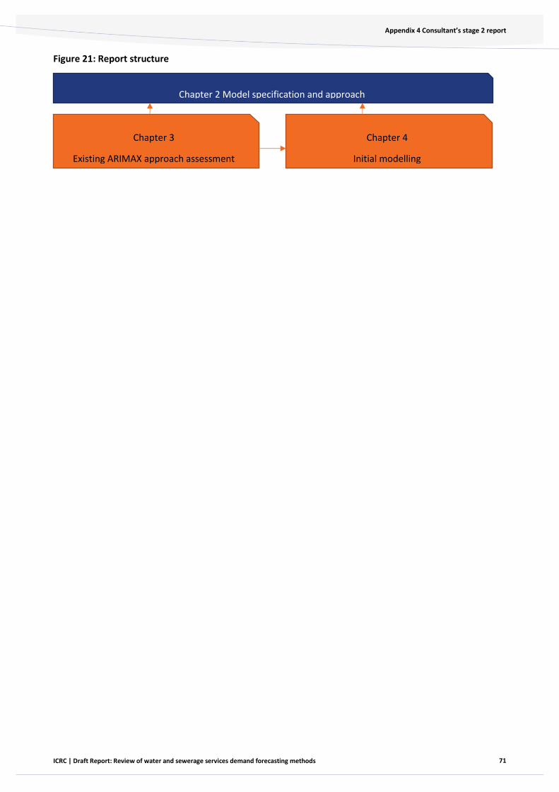
71
Appendix 4 Consultant’s stage 2 report
ICRC | Draft Report: Review of water and sewerage services demand forecasting methods
Figure 21: Report structure
Chapter 2 Model specification and approach
Chapter 3
Existing ARIMAX approach assessment
Chapter 4
Initial modelling
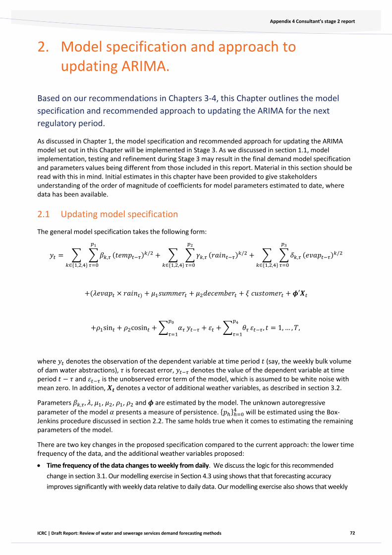
72
Appendix 4 Consultant’s stage 2 report
ICRC | Draft Report: Review of water and sewerage services demand forecasting methods
2. Model specification and approach to updating ARIMA.
Based on our recommendations in Chapters 3-4, this Chapter outlines the model
specification and recommended approach to updating the ARIMA for the next
regulatory period.
As discussed in Chapter 1, the model specification and recommended approach for updating the ARIMA model set out in this Chapter will be implemented in Stage 3. As we discussed in section 1.1, model implementation, testing and refinement during Stage 3 may result in the final demand model specification and parameters values being different from those included in this report. Material in this section should be read with this in mind. Initial estimates in this chapter have been provided to give stakeholders understanding of the order of magnitude of coefficients for model parameters estimated to date, where data has been available.
2.1 Updating model specification
The general model specification takes the following form:
𝑦𝑡 = ∑ ∑ 𝛽𝑘,𝜏
𝑝1
𝜏=0
(𝑡𝑒𝑚𝑝𝑡−𝜏)𝑘/2
𝑘∈{1,2,4}
+ ∑ ∑ 𝛾𝑘,𝜏
𝑝2
𝜏=0
(𝑟𝑎𝑖𝑛𝑡−𝜏)𝑘/2
𝑘∈{1,2,4}
+ ∑ ∑ 𝛿𝑘,𝜏
𝑝3
𝜏=0
(𝑒𝑣𝑎𝑝𝑡−𝜏)𝑘/2
𝑘∈{1,2,4}
+(𝜆𝑒𝑣𝑎𝑝𝑡 × 𝑟𝑎𝑖𝑛𝑡) + 𝜇1𝑠𝑢𝑚𝑚𝑒𝑟𝑡 + 𝜇2𝑑𝑒𝑐𝑒𝑚𝑏𝑒𝑟𝑡 + 𝜉 𝑐𝑢𝑠𝑡𝑜𝑚𝑒𝑟𝑡 + 𝝓′𝑿𝑡
+𝜌1sin𝑡 + 𝜌2cosin𝑡 + ∑ 𝛼𝜏
𝑝0
𝜏=1𝑦𝑡−𝜏 + 휀𝑡 + ∑ 𝜃𝜏
𝑝4
𝜏=1휀𝑡−𝜏, 𝑡 = 1, … , 𝑇,
where 𝑦𝑡 denotes the observation of the dependent variable at time period 𝑡 (say, the weekly bulk volume of dam water abstractions), 𝜏 is forecast error, 𝑦𝑡−𝜏 denotes the value of the dependent variable at time period 𝑡 − 𝜏 and 휀𝑡−𝜏 is the unobserved error term of the model, which is assumed to be white noise with mean zero. In addition, 𝑿𝒕 denotes a vector of additional weather variables, as described in section 3.2.
Parameters 𝛽𝑘,𝜏, 𝜆, 𝜇1, 𝜇2, 𝜌1, 𝜌2 and 𝝓 are estimated by the model. The unknown autoregressive
parameter of the model 𝛼 presents a measure of persistence. {𝑝ℎ}ℎ=04 will be estimated using the Box-
Jenkins procedure discussed in section 2.2. The same holds true when it comes to estimating the remaining parameters of the model.
There are two key changes in the proposed specification compared to the current approach: the lower time frequency of the data, and the additional weather variables proposed:
• Time frequency of the data changes to weekly from daily. We discuss the logic for this recommended
change in section 3.1. Our modelling exercise in Section 4.3 using shows that that forecasting accuracy
improves significantly with weekly data relative to daily data. Our modelling exercise also shows that weekly

73
Appendix 4 Consultant’s stage 2 report
ICRC | Draft Report: Review of water and sewerage services demand forecasting methods
data performs comparatively better than monthly data. Therefore, at this stage, our recommended
specification is the weekly data model.
• Include additional weather variables. We discuss the logic for this recommended change to model
specification in section 3.2. Our modelling exercise in Section 4.2 shows that additional weather variables
improve the forecasting accuracy of the model using monthly data, but may have little effect in a weekly
model. However, at this stage, our recommendation is to retain these additional weather variables until final
refinement and testing are done to identify the final model specification that best fits the data.
The variables for the weekly form of the model are described in Error! Reference source not found. along with data sources. Section 4.4 reports point estimates of the parameters for the selected model corresponding to the weekly observations and Appendix A1.2 includes detailed results and estimated parameters for the updated model with daily, weekly and monthly data, respectively.
Table 6: Updated model variables for the weekly form of the model and data source
Variable Description Reasoning Data Source
𝒚𝒕, Dam
abstractions Dam abstractions during a previous week
Dam abstractions are related over time. This is a function of the ARIMA model and is calculated using the model.
Provided by Icon Water
𝐭𝐞𝐦𝐩 Average of daily
maximum temperatures
(degrees Celsius) during
a week
Hot periods will result in more water
abstractions to meet increasing water
demand by customers
Bureau of Meteorology
for the Canberra Airport
station.
𝐫𝐚𝐢𝐧 Average daily rainfall
(mm) during a week
Rainy periods will result in less water
abstractions because part of customer’s
water demand will be met by rain (e.g.
less water required for plants during rainy
periods)
𝐞𝐯𝐚𝐩 Average daily
evaporation during a
week
High evaporation rates will result in more
water abstractions to meet higher
irrigation requirements for
plants/gardens as they dry.
Bureau of Meteorology
for the Burrinjuck Dam
station
𝐜𝐮𝐬𝐭𝐨𝐦𝐞𝐫 Icon water customer
connections at the end
of a week
More customers will increase water
demand, and will require more water
abstractions
Provided by Icon Water
𝑿𝒕, Additional
weather
variables to
capture the
effect of
extreme
weather
conditions on
dam
abstractions
• Number of days where daily temperature exceeded 30 °C or 35 °C in a week
More days with extreme high
temperature will result in more dam
abstractions.
Bureau of Meteorology
for the Canberra Airport
station and Bureau of
Meteorology for the
Burrinjuck Dam station • Number of days without rain in a week
More days without rain will result in more
dam abstractions.
• Interaction effect between rain*evap
High levels of evaporation and low levels
of rainfall is likely to be related to higher
demand for water

74
Appendix 4 Consultant’s stage 2 report
ICRC | Draft Report: Review of water and sewerage services demand forecasting methods
Variable Description Reasoning Data Source
𝐬𝐢𝐧 Sine and cosine
functions.
These are included to account for
seasonality (systematic, repetitive,
periodic fluctuations in dam abstractions
over the course of a week)
Self-defined
𝐜𝐨𝐬𝐢𝐧
Moving
average
component
Forecast error of dam
abstractions for the
previous week (weeks)
This is a function of the ARIMA model and
is calculated using the model.
Self-defined
In addition to the above explanatory variables, it is worth considering additional weather variables related to
evaporation, soil moisture index and humidity. Both variables are available in the NARCLiM database, to be
discussed below.
As discussed in more detail in sections 3.1, 3.4, and 3.7 the updated model specification better accounts for future changes in climate, demographics (e.g. population projections):
• Lower frequency data potentially avoid a clash between modelling climate change adaptation and predictive
ability over longer horizons, in that there is a plausible range of values for the autoregressive parameter that
is consistent with both.
• Computing forecasts of water installations based on ACT population projections produced by the Australian
Government’s Centre for Population has the advantage that these projections are up-to-date and include the
impact of Covid-19 and resulting border closures on future population growth. In contrast, population (or
water installation) projections based on past data, prior to 2020-21, do not consider the effect of Covid-19,
and therefore they are likely to be highly inaccurate. We understand the ICRC is considering using the ACT
Government’s population projections which accounts for future development activities in ACT and is being
updated to account for the effect of Covid-19.
2.2 Steps to ensure model and parameters are statistically sound
There are a number of steps that will be implemented in Stage 3 to ensure the model and parameters are statistically sound, and to confirm the final model specification.
Model selection
Model selection to determine the best-fit will be implemented in Stage 3 using the standard Box-Jenkins
procedure. The Box-Jenkins procedure involves:
1. Identification. This step involves determining the order of the model required (p, d, and q) to capture the
salient dynamic features of the data. This step mainly relies on the use of graphical procedures (plotting the
series, the ACF (autocorrelation function) and PACF (partial ACF), etc).
2. Estimation and Selection. This step involves estimation of the parameters of the different models (using step 1)
and proceeds to a first selection of models using information criteria, such as AIC and BIC. Model selection will
also be informed at this stage by examining the accuracy of aggregate (annual) in-sample forecasts obtained
during the validation period. In-sample forecast accuracy will be assessed using the MAPE and the RMSPE.

75
Appendix 4 Consultant’s stage 2 report
ICRC | Draft Report: Review of water and sewerage services demand forecasting methods
3. Diagnostic Checking. This step involves determining whether the model(s) specified and estimated are
adequate using residual diagnostics. In particular, the fitted models will be checked by considering plots, as well as
the autocorrelations of the residual series (the series of residual, or error, values). If necessary, these steps may be
applied iteratively until step 3 does not produce any improvement in the model.
Finally, aggregate (annual) out-of-sample forecasts will be produced for each financial year of the next regulatory
period.
2.3 Implementation of model changes
To update the ARIMAX model with the recommended changes, we recommend using actual data corresponding to the period July 2006 to June 2021. The training sample could be the period July 2006 -June 2018. The validation period will correspond to the period July 2018 -June 2021. Subsequently, out-of-sample forecasts of total abstractions will be obtained for each year during the next regulatory period.
For the training and validation periods, the data sources will be mostly consistent with those used by the existing approach of Icon Water. As shown in Error! Reference source not found. the dependent variable will be actual dam abstractions, made available to us by Icon Water. Data on temperature\rain-related variables are publicly available by the Bureau of Meteorology for the Canberra Airport station. Data on evaporation are publicly from the same source for the Burrinjuck Dam station. Data on customer numbers are made available to us by Icon Water.
Initial ARIMAX models should be estimated using weekly and monthly observations, using the model selection steps discussed in section 2.3.
To implement out-of-sample forecasts of total abstractions, we need forecasts of weather conditions during the next few years. Previously, South Eastern Australian Climate Initiative (SEACI) data was used for conditioning past climate data with future climate projections. For this model update we recommend mostly relying on the NARCLiM database, a multi-agency research project between the NSW and ACT governments and the Climate Change Research Centre at the University of NSW.
The NARCliM project has produced a suite of twelve regional climate projections for south-east Australia, including Canberra, spanning the range of likely future changes in climate. NARCliM is explicitly designed to sample a large range of possible future climates, and provides daily forecasts of weather conditions that go as far as 2030 in their so-called “Near Future” setup. Weekly and monthly weather variables will be constructed from daily NARCliM forecasts.
Out-of-sample predictions of total abstractions will be obtained using dynamic forecasting. This step will produce a "mean forecast” by averaging weather variables across the 12 different regional climate projections, produced by NARCLiM for the near future (up to 2028). To check the sensitivity of the forecasts to alternative future weather scenarios, additional weather forecasts will be used based on different quantiles of the distribution of the climate projections. Additional forecasts should be produced based on each of the twelve individual climate projections, which will then be summarised using mean, median and different quantiles.
76
Appendix 4 Consultant’s stage 2 report
ICRC | Draft Report: Review of water and sewerage services demand forecasting methods
3. Assessment on the current ARIMA approach
The Auto-Regressive Integrated Moving Average model, or ARIMA for short, is a
popular statistical model used to analyse and forecast time series data. In this
section we outline our assessment of the current ARIMA methodology.
An Auto-Regressive Integrated Moving Average model combines an autoregressive (AR) model with a moving average (MA) model. An AR model uses past values of the forecast variables as predictors. A MA model uses past values of forecasted errors.
The main objective in ARIMA is to model autocorrelations in the data, i.e. the dependence of the observations over time. When the series are non-stationary (or “integrated”) such that the autocorrelations of the data depend on the time at which the series is observed, ARIMA differences the data to allow the series to become stationary. Typically, specification of ARIMA models relies on the so-called Box-Jenkins method, which is a systematic process for identifying, fitting, and checking time series models.
For high-frequency data, such as with daily observations, ARIMA also allows modelling seasonal variation, by augmenting the model with additional seasonal terms. When the seasonal patterns are non-stationary, ARIMA can make use of seasonal differencing to allow the series to become seasonally stationary.
ARIMA can also incorporate exogenous control variables. In regression analysis, the standard notation used for such variables is given by “x”. Hence, ARIMA models with exogenous regressors are commonly known as ARIMAX models.
ARIMAX models have been used to analyse and forecast daily observations of ACT bulk water volumes, obtained from dam abstractions. The daily abstractions data are aggregated into monthly totals comparable in coverage to the monthly billed consumption data. Subsequently, the regression estimate of the ratio of historical billed consumption to abstractions is applied to the annual abstractions to calculate a forecast of Icon Water annual billed sales. The annual billed sales forecast is split into Tier 1 and Tier 2 consumption, based on the historical relationship between water consumption per installation and the observed proportion of total sales falling into the Tier 1 category.
Compared to other commercial applications of ARIMA to support demand forecasting for regulated utilities we have reviewed, and based on our review of Icon Water’s documentation, the quality of implementation of the method is high, and the various steps undertaken have been documented well. We discuss these issues in more detail in our Stage 1 advice available on the ICRC website here.
In the next section we identify some key issues and identify recommendations to further improve the existing ARIMA methodology. These recommendations reflect and extend on observations made in our Stage 1 review.
3.1 Time frequency (Short-term versus long-term forecasts using daily data)
3.1.1 Key issues
The existing ARIMA methodology makes use of daily observations on total volumes of water from dam abstractions. This approach is well suited for producing short-term forecasts of dam abstractions, such as one day, two days or one week ahead.

77
Appendix 4 Consultant’s stage 2 report
ICRC | Draft Report: Review of water and sewerage services demand forecasting methods
However, daily data are not best suited for producing forecasts over longer horizons, such as one month ahead, or multiple years ahead. There are three main reasons why daily data are not best suited for producing forecasts over longer horizons:
• the prediction interval is likely to be much wider for longer horizons than it is for shorter ones. A common
feature of prediction intervals is that they typically increase in length as the forecast horizon increases,
particularly so for dynamic forecasting. Dynamic forecasting uses the forecast (as opposed to the actual)
value of the lagged dependent variable to obtain the forecasts of abstractions. Therefore, any forecast errors
tend to compound over time. With daily data, one needs to forecast ahead several (hundreds of) time
periods and so any error in forecasting the lagged dependent variable can feed into the distant future.
• daily observations are heavily influenced by intra-week (seasonal) variation. Thus, models based on daily
data estimate parameters that may not be relevant for (or even distort) forecasts over long-term horizons.
For example, models based on daily data require taking into account the impact of the day of the week on
total abstractions (e.g. whether it is a weekday or a weekend). Such intra-week seasonality will not be
important when forecasting abstractions over long time horizons. Essentially, the existing approach using
daily observations requires estimation of day-specific parameters, which are not relevant for longer term
forecasting.
• daily data give rise to a clash between modelling climate change adaptation and forecasting ability over
longer horizons. Human behaviour is intrinsically dynamic. For example, because of the force of habit and
technical constraints (such as the need to install water saving devices), households may not change their
water consumption patterns instantaneously, only over time. Imperfect knowledge and uncertainty may also
contribute to persistence, or a delayed response to shocks by decision makers.12
In dynamic regression models, the costs of instantaneous adjustment are often characterised by the magnitude of the autoregressive parameters.
To illustrate, consider a simple Auto-Regressive Distributed Lag (ARDL) model of order 1 in the autoregressive component and 0 in the distributed lag (i.e. an ARDL(1,0) model):
𝑦𝑡
= 𝛼𝑦𝑡−1
+ 𝛽𝑥𝑡 + 휀𝑡; 𝑡 = 𝑡, … , 𝑇, (1)
where 𝑦𝑡 denotes (say) the bulk volume of daily dam water release at time period 𝑡, 𝑦𝑡−1 denotes the value of the total volume of dam water release during the previous day, 𝑥𝑡 denotes (say) temperature at time period 𝑡, and 휀𝑡 is the unobserved error term of the model, which is assumed to be white noise with mean
zero, such that 𝐸[휀𝑡|𝑦𝑡−1,𝑥𝑡] = 0. Finally, 𝛼 and 𝛽 denote the unknown parameters of the model. The
autoregressive component of the model above accounts for the fact that consumers may take time to adjust fully to long-lasting (or permanent) changes in climate, such as temperature. The more time it takes to adjust to climate change, the more “persistent” the variable of interest (total abstractions) is.
Suppose that temperature goes up by one unit and, on average, it stays to that level thereafter due to climate change. The short-term (or immediate) effect of the change in temperature on water consumption
—————
12 See e.g. Bun and Sarafidis (2015), ‘Dynamic Panel Data Models’. In B. Baltagi (eds.) Oxford Handbook of Panel Data, Oxford
University Press, Ch. 3, pp. 76-110.

78
Appendix 4 Consultant’s stage 2 report
ICRC | Draft Report: Review of water and sewerage services demand forecasting methods
is given by 𝛽. The long-term (or total) effect over time is given by 𝛽/(1 − 𝛼). The speed of adjustment towards the total effect is given by (1 − 𝛼).
The smaller (larger) the value of 𝛼 is, the higher (lower) the speed of adjustment. For instance, when for 𝛼 = 0.95, it takes 45 time periods (i.e. 45 days, when daily data are used) for 90% of the long-term effect to be realised. This means that the dependent variable of the model (total abstractions) is highly persistent. On other hand, when 𝛼 = 0.5, it takes 4 time periods (4 days) for 90% of the long-term effect to be realised.13 That is, a value of 𝛼 equal to 0.5 implies that consumers adapt almost completely to a permanent unit change in climatic conditions within 4 days. Such a rate of adaptation is unrealistic. Therefore, when it comes to modelling climate change adaptation, high values of 𝛼 would be more plausible.
Unfortunately, as shown in Section A1.1, with high values of α, it becomes more difficult to forecast accurately future values of yt. In particular, the accuracy of the forecasts can diminish considerably once one deviates sufficiently from one- or two-day ahead forecasts.
The above discussion illustrates a tension in the use of daily data to (i) forecast long-term water consumption and (ii) model climate change adaptation. On the one hand, the use of daily data for modelling long-term adaptation to climate change promises the most hope when the value of the autoregressive parameter (denoted by 𝛼) is high (and hence, the speed of adjustment is low). On the other hand, it is precisely in these contexts, where the magnitude of 𝛼 is close to unity, that the predicted value of water consumption in the medium to long-term will be associated with a large forecast error. In other words, while high values of 𝛼 offer the most hope to capture the dynamics of climate change adaptation using daily data, these are the values most likely associated with larger forecast errors.
3.1.2 Our recommendation
We recommend making use of lower time frequency data in the ARIMA model. Weekly, monthly or quarterly time series may be useful in providing additional information relative to the use of daily data alone. We illustrate how this approach can improve the forecasting accuracy of the model in section 4.
The use of lower frequency data can alleviate many of these issues. For example, intra-week seasonal variation will average out with weekly or monthly data, thus avoiding estimating parameters that are irrelevant for forecasting over long horizons.
Moreover, forecasting analysis based on lower frequency data can avoid a clash between climate change adaptation and predictive ability over longer horizons, in that there is a plausible range of values for the autoregressive parameter that is consistent with both.
—————
13 To illustrate, suppose that 𝛽 = 3 and 𝛼 = 0.5. The long-term impact of a unit increase in 𝑥 equals 𝛽/(1 − 𝛼) = 3/(1 − 0.5) = 6,
or 6 units of total water volume per day. The speed of adjustment equals 1 − 0.5 = 0.5. A unit increase in temperature is expected
to increase water consumption by 3 units the first day (or 0.5 of the total effect, which equals 6). During the second day, water
consumption will increase by another 1.5 units ((6 − 3) × 0.5). During the third day, water consumption will increase by another
0.75 units ((6 − 4.5) × 0.5), and so on. Note that it takes 4 time periods for 90% of the total effect to be realised.
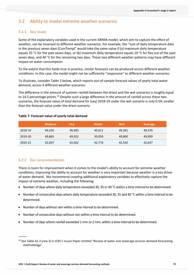
79
Appendix 4 Consultant’s stage 2 report
ICRC | Draft Report: Review of water and sewerage services demand forecasting methods
3.2 Ability to model extreme weather scenarios
3.2.1 Key issues
Some of the explanatory variables used in the current ARIMA model, which aim to capture the effect of weather, can be invariant to different weather scenarios. For example, the “sum of daily temperature data in the previous seven days (CumTemp)” would take the same value if (a) maximum daily temperature equals 25 °C for the past seven days, or (b) maximum daily temperature equals 19 °C for five out of the past seven days, and 40 °C for the remaining two days. These two different weather patterns may have different impact on water consumption.
To the extent that this holds true in practice, similar forecasts can be produced across different weather conditions. In this case, the model might not be sufficiently “responsive” to different weather scenarios.
To illustrate, consider Table 3 below, which reports out-of-sample forecast values of yearly total water demand, across 4 different weather scenarios.
The difference in the amount of summer rainfall between the driest and the wet scenarios is roughly equal to 14.5 percentage points.14 Despite such a large difference in the amount of rainfall across these two scenarios, the forecast value of total demand for (say) 2018-19 under the wet scenario is only 0.5% smaller than the forecast value under the driest scenario.
Table 7: Forecast value of yearly total demand
Medium Dry Driest Wet Average
2018-19 49,426 49,483 49,611 49,361 49,470
2019-20 49,865 49,922 50,050 49,800 49,909
2020-21 42,607 42,662 42,776 42,542 42,647
3.2.2 Our recommendation
There is room for improvement when it comes to the model’s ability to account for extreme weather conditions. Improving the ability to account for weather is very important because weather is a key driver of water demand. We recommend creating additional explanatory variables to effectively capture the impact of extreme weather, including the following:
• Number of days where daily temperature exceeded 30, 35 or 40 °C within a time interval to be determined.
• Number of consecutive days where daily temperature exceeded 30, 35 and 40 °C within a time interval to be
determined.
• Number of days without rain within a time interval to be determined.
• Number of consecutive days without rain within a time interval to be determined.
• Number of days where rainfall exceeded 1 mm or 2 mm, within a time interval to be determined.
—————
14 See Table A2.3 (row 3) in ICRC’s Issues Paper entitled “Review of water and sewerage services demand forecasting methodology”.
80
Appendix 4 Consultant’s stage 2 report
ICRC | Draft Report: Review of water and sewerage services demand forecasting methods
• Number of days where rainfall was less than or equal to 1 mm or 2 mm, within a time interval to be
determined.
Many of these variables have been applied successfully in forecasting water demand elsewhere; see e.g. Barker et al (2020) for a recent study in the Australian context.15
In addition to the above explanatory variables, it is worth considering additional weather variables related to evaporation, in particular, soil moisture content and humidity. Both variables are available in the NARCLiM database, which will be discussed below.
3.3 Future climatic scenarios
3.3.1 Key issues
Currently, future climatic scenarios are incorporated into the model in two different ways. When it comes to temperature, future trends are estimated using simple regression analysis of daily temperature on a linear trend. On the other hand, for rainfall and evaporation, 4 different scenarios are employed based on data from the South Eastern Australian Climate Initiative (SEACI 2012); namely a medium scenario, a wet scenario, a dry and a driest one.
Our view is that this strategy may not the most suitable approach for future climatic scenarios for several reasons:
• it is not clear that the trend in temperature is linear. In fact, preliminary analysis using data for Burrinjuck
Dam NSW (Station Number 73007), indicates that the trend is highly nonlinear.
• the trend estimate appears to be highly sensitive to the estimation period (i.e. sample) used in the
regression.
• temperature is highly correlated with rainfall and evaporation. High levels of evaporation and low levels of
rainfall may be accompanied by high levels of temperature. However, the current climate analysis does not
allow for that. For instance, the driest scenario over the summer involves 6% less rain, 4% higher evaporation,
yet temperature does not adjust accordingly. This can distort the effectiveness of the model to capture
different climatic scenarios.
3.3.2 Our recommendation
We recommend the construction of future climatic scenarios using a single database, such as NSW and ACT Regional Climate Modelling (NARCLiM).
The NARCLiM database provides a more up-to-date source of climate change data and would account for changes in key weather conditions, such as temperature and rainfall. We note that this approach is supported by Icon Water, as outlined in its submission to the ICRC’s demand forecasting issues paper16. We will consider this database as well in Stage 3.
—————
15 Barker, A., Pitman, A., Evans, J., Spaninks, F., Uthayakumaran, L. (2020). Drivers of future water demand in Sydney, Australia: examining the contribution from population and climate change. Journal of Water and Climate Change 12(2), 1168-1183.
16 Icon Water, Response to Demand forecasting Issues Paper, 9 July 2021.

81
Appendix 4 Consultant’s stage 2 report
ICRC | Draft Report: Review of water and sewerage services demand forecasting methods
3.4 Population projections
3.4.1 Key issues
Under the current approach, forecasts of water installations are computed based on historical growth rates of the same variable. This implies that these forecasts do not consider the impact of Covid-19 and the resulting border closures on future customer growth for Icon Water.
Ignoring the impact of Covid-19 may lead to significantly higher forecasts of water installations than actual ones. For example, we note that ACT’s annual population forecasts during the period 2021-22 to 2030-31, updated by the Australian Government’s Centre for Population to account for Covid-19, are on average 2.3% lower than the previous forecasts made without taking into account the effect of Covid-19, as shown in Table 8.
Table 8 Population projections ACT under pre and post COVID scenarios
Year Post-Covid 19 scenario Pre-Covid 19 scenario Percentage difference
2021-22 431,400 436,000 -1.10%
2022-23 432,800 440,900 -1.80%
2023-24 435,800 445,700 -2.20%
2024-25 439,900 450,500 -2.40%
2025-26 444,000 455,200 -2.50%
2026-27 448,000 459,800 -2.60%
2027-28 452,000 464,200 -2.60%
2028-29 455,900 468,500 -2.70%
2029-30 459,700 472,700 -2.80%
2030-31 463,400 476,700 -2.80%
3.4.2 Our recommendation
To account for the impact of Covid-19, we recommend adopting the following two-step procedure. In the first step, historical data of Icon Water’s water installations are regressed on ACT’s population. This allows one identifying the relationship between the two variables. In the second stage, future water installations are imputed based on the aforementioned regression model using as predictor the Covid-19-updated population forecasts for ACT. We understand the ICRC is considering using the ACT Government’s population projections which accounts for future development activities in ACT and is being updated to account for the effect of Covid-19.17 If these updated ACT Government population projections are not available at the time of stage 3 finalisation, we recommend using population forecasts for ACT produced by the Australian Government’s Centre for Population. An important consideration is to ensure that the ACT population forecasts account for the impact of Covid-19.
—————
17 https://www.treasury.act.gov.au/snapshot/demography/act
82
Appendix 4 Consultant’s stage 2 report
ICRC | Draft Report: Review of water and sewerage services demand forecasting methods
3.5 Forecasting accuracy
3.5.1 Key issues
The out-of-sample forecasting performance of the model needs to be assessed using well-established measures of accuracy, such as the Root Mean Squared Error (RMSE), the Root Mean Squared Percentage Error (RMSPE) and the Mean Absolute Per cent Error (MAPE). RMSE/RMSPE and MAPE will be computed based on the average value of the (squared or absolute, respectively) difference between the yearly forecast and actual values.
Currently, out-of-sample forecasting performance has been accessed in terms of the Mean Per cent Error (hereafter, MPE). This denotes the average value of the difference (neither squared, nor absolute) between the yearly forecast and the actual value. There are three years available for validation, namely 2018-19 to 2020-21.
The MPE is a useful measure for checking forecasting bias. That is, in the present context it may help to examine the extent to which yearly forecast errors roughly balance out over the relevant period of time, which is currently set to three years.
On the other hand, the MPE is less useful as a measure of forecasting accuracy. This is mainly because the MPE can fail to distinguish between really good models and really bad ones.
To illustrate, consider two competing forecasting models, A and B. Suppose that forecasting performance is assessed over two years. In year 1, Model A overpredicts actual demand by 100%, whereas in year 2 Model A underpredicts demand by 99%. On the other hand, Model B overpredicts actual demand by 1% in year 1 and it is spot on in its prediction in year 2 (i.e., the forecasting error is zero). As it turns out, for both Model A and Model B, the value of MPE equals 1%. That is, according to this measure, both A and B perform equally well. That is, of course, not true.
In addition, since MPE is computed over a small number of years, the average forecast error can be sensitive to one or two forecast errors (outliers), which can be due to e.g. extreme weather conditions. If such outliers in yearly forecasts are overlooked and not studied carefully, the performance of the model may remain sensitive. From a statistical point of view, MPE is a random variable with unknown finite sample properties. It may take a single large forecast error to substantially distort the predictions.
3.5.2 Our recommendation
Our recommendation is that effort should be made to improve forecasts on an annual basis, not just over the regulatory period. The reporting of accuracy performance should be reported using established accuracy measures, such as the RMSE and the MAPE. Improving on the yearly forecasts and complementing the MPE measure with more appropriate accuracy measures will increase transparency, and may lead to a better forecasting model over each five-year regulatory period. We have used these accuracy measures in our analysis in section 4.
3.6 Model uncertainty vs uncertainty in predicting weather conditions.
3.6.1 Key issues
When it comes to the accuracy of out-of-sample forecasts, the performance of the model largely depends on two factors: the accuracy of predicting weather conditions; and the accuracy of the model in terms of predicting total abstractions conditional on weather being known. The former reflects uncertainty due to the inherent difficulty of predicting future weather, and the latter reflects model uncertainty.

83
Appendix 4 Consultant’s stage 2 report
ICRC | Draft Report: Review of water and sewerage services demand forecasting methods
While the former might be unavoidable, since weather is difficult to predict, the latter needs to be carefully studied. Ideally, when weather conditions are predicted correctly, no matter what these conditions are, the forecast values should be close to actual ones, despite any peaks or troughs observed on actual weather.
It appears that the bulk of forecast errors in the current model is attributed to “unusual weather conditions”. For this reason, we consider it is important that the forecasting analysis makes a distinction between uncertainty that is due to predicting future weather conditions, and model uncertainty.
3.6.2 Our recommendation
Efforts should be made to distinguish between model uncertainty and uncertainty due to unpredictability of weather conditions. Specifically, when testing forecasting accuracy of the model ex-post, we recommend isolating model uncertainty by producing forecasts of total abstractions based on predicted weather conditions, and also forecasts in terms of actual weather conditions. In the latter case, the error in predicting weather is zero, and therefore any discrepancies between forecast and actual values of total abstractions can be attributed to model uncertainty.
To measure out-of-sample forecast accuracy, it is useful to produce two values of MAPE, one based on actual weather conditions and one based on predicted weather conditions. The magnitude of the former reflects model uncertainty. The magnitude of the difference between the two values of MAPE reflects the impact of weather uncertainty. Note that ex ante, the latter is the only feasible option.
3.7 Estimation and lag order selection
3.7.1 Key issues
Under the existing approach, identification of the number of lags to be used in terms of weather variables is undertaken outside the ARIMA model, based on some form of pre-whitening. This can undermine simplicity, as well as estimation efficiency.
3.7.2 Our recommendation
We recommend that identification and model selection for the ARIMA model is undertaken based on the Box-Jenkins procedure.
This may increase estimation efficiency and improve the transparency of the preferred specification. For this reason, it is advised not to use pre-whitening of the observations (pre-whitening removes autocorrelation and trends from the cross-correlation function).
3.8 Policy adjustments
It is desirable to be able to accommodate in the forecasting model future policy changes, such as sustainable diversion limits. To the extent that there are data available, such policy changes should be incorporated within the model prior to producing the forecasts. Otherwise, post-model adjustments may be the only feasible method within the ARIMA approach. Alternatively, consumer-specific billed water data may be useful in identifying the impact of policy changes.
3.9 Terminology
We recommend referring to the model as “ARIMAX”, since the model uses exogenous variables.
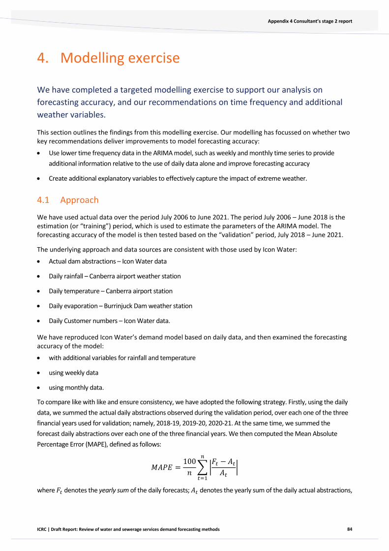
84
Appendix 4 Consultant’s stage 2 report
ICRC | Draft Report: Review of water and sewerage services demand forecasting methods
4. Modelling exercise
We have completed a targeted modelling exercise to support our analysis on
forecasting accuracy, and our recommendations on time frequency and additional
weather variables.
This section outlines the findings from this modelling exercise. Our modelling has focussed on whether two key recommendations deliver improvements to model forecasting accuracy:
• Use lower time frequency data in the ARIMA model, such as weekly and monthly time series to provide
additional information relative to the use of daily data alone and improve forecasting accuracy
• Create additional explanatory variables to effectively capture the impact of extreme weather.
4.1 Approach
We have used actual data over the period July 2006 to June 2021. The period July 2006 – June 2018 is the estimation (or “training”) period, which is used to estimate the parameters of the ARIMA model. The forecasting accuracy of the model is then tested based on the “validation” period, July 2018 – June 2021.
The underlying approach and data sources are consistent with those used by Icon Water:
• Actual dam abstractions – Icon Water data
• Daily rainfall – Canberra airport weather station
• Daily temperature – Canberra airport station
• Daily evaporation – Burrinjuck Dam weather station
• Daily Customer numbers – Icon Water data.
We have reproduced Icon Water’s demand model based on daily data, and then examined the forecasting accuracy of the model:
• with additional variables for rainfall and temperature
• using weekly data
• using monthly data.
To compare like with like and ensure consistency, we have adopted the following strategy. Firstly, using the daily
data, we summed the actual daily abstractions observed during the validation period, over each one of the three
financial years used for validation; namely, 2018-19, 2019-20, 2020-21. At the same time, we summed the
forecast daily abstractions over each one of the three financial years. We then computed the Mean Absolute
Percentage Error (MAPE), defined as follows:
𝑀𝐴𝑃𝐸 =100
𝑛∑ |
𝐹𝑡 − 𝐴𝑡
𝐴𝑡|
𝑛
𝑡=1
where 𝐹𝑡 denotes the yearly sum of the daily forecasts; 𝐴𝑡 denotes the yearly sum of the daily actual abstractions,
85
Appendix 4 Consultant’s stage 2 report
ICRC | Draft Report: Review of water and sewerage services demand forecasting methods
and 𝑛 = 3 because the validation period consists of 3 financial years. Because the MAPE is a percentage of
absolute forecast errors, it is easier to understand than many other measures of forecasting accuracy, such as the
Root Mean Squared Error (RMSE). For example, if the MAPE equals 3, then, on average, the annual forecast is off
by 3%.
We have also used an alternative measure, the Root Mean Squared Percentage Error (RMSPE). This is similar to
the well-known RMSE, except it is expressed in percentage terms. The RMSPE is defined as follows:
𝑅𝑀𝑆𝑃𝐸 = √1
𝑛∑ [100 × (
𝐹𝑡−𝐴𝑡
𝐴𝑡)]
2𝑛𝑡=1 .
Since our emphasis lies in comparing the forecasting accuracy of the various models, we have computed forecasts
for abstractions based on actual weather conditions during the period 2018-2021. This means that the forecasting
accuracy of all models presented here will be higher than that reported by Icon Water, even if the benchmark
model is identical to theirs.
Subsequently, we have followed the same procedure for weekly and monthly data. In particular, we have used
the period July 2006 – June 2018 to estimate the ARIMAX model using weekly (monthly) observations. We have
obtained weekly (monthly) forecasts for the period July 2018 – June 2021. Finally, we summed the actual weekly
(monthly) abstractions and the forecast weekly (monthly) abstractions over each one of the three financial years
used for calibration; namely, 2018-19, 2019-20, 2020-21. We computed the MAPE and RMPSE again for these
models.
The benchmark ARIMAX model using daily observations has the same representation as that reported in Icon
Water’s 2018-23 price proposal to the ICRC18.
4.2 Explanatory variables for weather conditions
In our assessment of the current ARIMA model in Chapter 3 we noted that some of the explanatory variables used, which aim to capture the effect of weather, are invariant to different weather scenarios. We have therefore recommended creating additional explanatory variables to effectively capture the impact of extreme weather, including:
• Number of days where daily temperature exceeded 30, 35 or 40 °C within the previous week (month)
• Number of consecutive days where daily temperature exceeded 30, 35 and 40 °C within the previous week
(month)
• Number of days without rain within the previous week within the previous week (month)
• Number of consecutive days without rain within the previous week.
• Number of days where rainfall exceeded 1 mm or 2 mm, within the previous week (month)
• Number of days where rainfall was less than or equal to 1 mm or 2 mm, within the previous week (month).
• To simplify things, we have used least-squares regression to select which of these explanatory variables are
statistically significant. The following were found to be statistically significant:
—————
18 Icon Water, 2018-23 Price Proposal Attachment 4 - Demand Forecasts, Table 2-4.
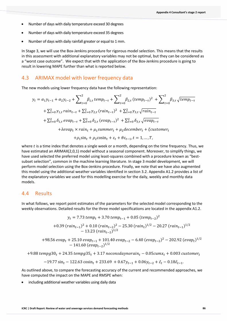
86
Appendix 4 Consultant’s stage 2 report
ICRC | Draft Report: Review of water and sewerage services demand forecasting methods
• Number of days with daily temperature exceed 30 degrees
• Number of days with daily temperature exceed 35 degrees
• Number of days with daily rainfall greater or equal to 1 mm.
In Stage 3, we will use the Box-Jenkins procedure for rigorous model selection. This means that the results in this assessment with additional explanatory variables may not be optimal, but they can be considered as a “worst case outcome”. We expect that with the application of the Box-Jenkins procedure is going to result in lowering MAPE further than what is reported below.
4.3 ARIMAX model with lower frequency data
The new models using lower frequency data have the following representation:
𝑦𝑡 = 𝛼1𝑦𝑡−1 + 𝛼2𝑦𝑡−2 + ∑ 𝛽1,𝜏
2
𝜏=0𝑡𝑒𝑚𝑝𝑡−𝜏 + ∑ 𝛽2,𝜏
2
𝜏=0(𝑡𝑒𝑚𝑝𝑡−𝜏)2 + ∑ 𝛽3,𝜏
2
𝜏=0√𝑡𝑒𝑚𝑝𝑡−𝜏
+ ∑ 𝛾1,𝜏2𝜏=0 𝑟𝑎𝑖𝑛𝑡−𝜏 + ∑ 𝛾2,𝜏
2𝜏=0 (𝑟𝑎𝑖𝑛𝑡−𝜏)2 + ∑ 𝛾3,𝜏
2𝜏=0 √𝑟𝑎𝑖𝑛𝑡−𝜏
+ ∑ 𝛿1,𝜏2𝜏=0 𝑒𝑣𝑎𝑝𝑡−𝜏 + ∑ 𝛿2,𝜏
2𝜏=0 (𝑒𝑣𝑎𝑝𝑡−𝜏)2 + ∑ 𝛿3,𝜏
2𝜏=0 √𝑒𝑣𝑎𝑝𝑡−𝜏
+𝜆𝑒𝑣𝑎𝑝𝑡 × 𝑟𝑎𝑖𝑛𝑡 + 𝜇1𝑠𝑢𝑚𝑚𝑒𝑟𝑡 + 𝜇2𝑑𝑒𝑐𝑒𝑚𝑏𝑒𝑟𝑡 + 𝜉𝑐𝑢𝑠𝑡𝑜𝑚𝑒𝑟𝑡
+𝜌1sin𝑡 + 𝜌2cosin𝑡 + 휀𝑡 + 𝜃휀𝑡−1, 𝑡 = 1, … , 𝑇,
where 𝑡 is a time index that denotes a single week or a month, depending on the time frequency. Thus, we have estimated an ARIMAX(2,0,1) model without a seasonal component. Moreover, to simplify things, we have used selected the preferred model using least-squares combined with a procedure known as “best-subset selection”, common in the machine learning literature. In stage 3 model development, we will perform model selection using the Box-Jenkins procedure. Finally, we note that we have also augmented this model using the additional weather variables identified in section 3.2. Appendix A1.2 provides a list of the explanatory variables we used for this modelling exercise for the daily, weekly and monthly data models.
4.4 Results
In what follows, we report point estimates of the parameters for the selected model corresponding to the weekly observations. Detailed results for the three model specifications are located in the appendix A1.2.
𝑦𝑡 = 7.73 𝑡𝑒𝑚𝑝𝑡 + 3.70 𝑡𝑒𝑚𝑝𝑡−1 + 0.05 (𝑡𝑒𝑚𝑝𝑡−2)2
+0.39 (𝑟𝑎𝑖𝑛𝑡−1)2 + 0.10 (𝑟𝑎𝑖𝑛𝑡−2)2 − 25.30 (𝑟𝑎𝑖𝑛𝑡)1/2 − 20.27 (𝑟𝑎𝑖𝑛𝑡−1)1/2
− 13.23 (𝑟𝑎𝑖𝑛𝑡−2)1/2
+98.56 𝑒𝑣𝑎𝑝𝑡 + 25.10 𝑒𝑣𝑎𝑝𝑡−1 + 101.40 𝑒𝑣𝑎𝑝𝑡−2 − 6.40 (𝑒𝑣𝑎𝑝𝑡−2)2 − 202.92 (𝑒𝑣𝑎𝑝𝑡)1/2
− 141.60 (𝑒𝑣𝑎𝑝𝑡−2)1/2
+9.88 𝑡𝑒𝑚𝑝𝑔30𝑡 + 24.35 𝑡𝑒𝑚𝑝𝑔35𝑡 + 3.17 𝑛𝑜𝑐𝑜𝑛𝑠𝑑𝑎𝑦𝑛𝑜𝑟𝑎𝑖𝑛𝑡 − 0.05𝑐𝑢𝑚𝑥𝑡 + 0.003 𝑐𝑢𝑠𝑡𝑜𝑚𝑒𝑟𝑡
−19.77 sin𝑡 − 122.63 cosin𝑡 + 233.69 + 0.67𝑦𝑡−1 + 0.06𝑦𝑡−2 + 휀�̂� − 0.18휀�̂�−1.
As outlined above, to compare the forecasting accuracy of the current and recommended approaches, we have computed the impact on the MAPE and RMSPE when:
• including additional weather variables using daily data
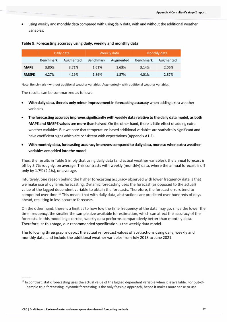
87
Appendix 4 Consultant’s stage 2 report
ICRC | Draft Report: Review of water and sewerage services demand forecasting methods
• using weekly and monthly data compared with using daily data, with and without the additional weather
variables.
Table 9: Forecasting accuracy using daily, weekly and monthly data
Daily data Weekly data Monthly data
Benchmark Augmented Benchmark Augmented Benchmark Augmented
MAPE 3.80% 3.71% 1.61% 1.63% 3.14% 2.06%
RMSPE 4.27% 4.19% 1.86% 1.87% 4.01% 2.87%
Note: Benchmark – without additional weather variables, Augmented – with additional weather variables
The results can be summarized as follows:
• With daily data, there is only minor improvement in forecasting accuracy when adding extra weather
variables
• The forecasting accuracy improves significantly with weekly data relative to the daily data model, as both
MAPE and RMSPE values are more than halved. On the other hand, there is little effect of adding extra
weather variables. But we note that temperature-based additional variables are statistically significant and
have coefficient signs which are consistent with expectations (Appendix A1.2).
• With monthly data, forecasting accuracy improves compared to daily data, more so when extra weather
variables are added into the model.
Thus, the results in Table 5 imply that using daily data (and actual weather variables), the annual forecast is off by 3.7% roughly, on average. This contrasts with weekly (monthly) data, where the annual forecast is off only by 1.7% (2.1%), on average.
Intuitively, one reason behind the higher forecasting accuracy observed with lower frequency data is that we make use of dynamic forecasting. Dynamic forecasting uses the forecast (as opposed to the actual) value of the lagged dependent variable to obtain the forecasts. Therefore, the forecast errors tend to compound over time.19 This means that with daily data, abstractions are predicted over hundreds of days ahead, resulting in less accurate forecasts.
On the other hand, there is a limit as to how low the time frequency of the data may go, since the lower the time frequency, the smaller the sample size available for estimation, which can affect the accuracy of the forecasts. In this modelling exercise, weekly data performs comparatively better than monthly data. Therefore, at this stage, our recommended specification is the weekly data model.
The following three graphs depict the actual vs forecast values of abstractions using daily, weekly and monthly data, and include the additional weather variables from July 2018 to June 2021.
—————
19 In contrast, static forecasting uses the actual value of the lagged dependent variable when it is available. For out-of-sample true forecasting, dynamic forecasting is the only feasible approach, hence it makes more sense to use.

88
Appendix 4 Consultant’s stage 2 report
ICRC | Draft Report: Review of water and sewerage services demand forecasting methods
Figure 22: Actual vs forecast volumes using daily data, July 2018 – June 2021
Figure 23: Actual vs forecast volumes using weekly data, July 2018 – June 2021
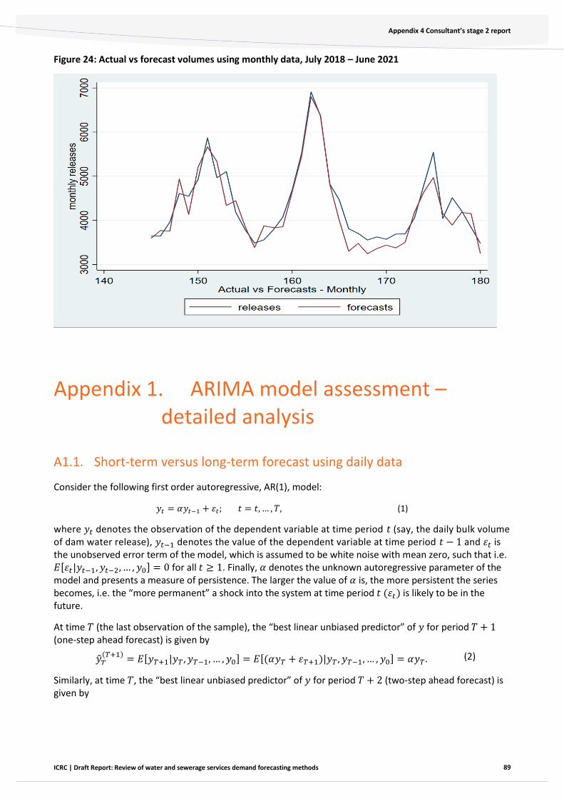
89
Appendix 4 Consultant’s stage 2 report
ICRC | Draft Report: Review of water and sewerage services demand forecasting methods
Figure 24: Actual vs forecast volumes using monthly data, July 2018 – June 2021
Appendix 1. ARIMA model assessment – detailed analysis
A1.1. Short-term versus long-term forecast using daily data
Consider the following first order autoregressive, AR(1), model:
𝑦𝑡 = 𝛼𝑦𝑡−1 + 휀𝑡; 𝑡 = 𝑡, … , 𝑇, (1)
where 𝑦𝑡 denotes the observation of the dependent variable at time period 𝑡 (say, the daily bulk volume of dam water release), 𝑦𝑡−1 denotes the value of the dependent variable at time period 𝑡 − 1 and 휀𝑡 is the unobserved error term of the model, which is assumed to be white noise with mean zero, such that i.e. 𝐸[휀𝑡|𝑦𝑡−1, 𝑦𝑡−2, … , 𝑦0] = 0 for all 𝑡 ≥ 1. Finally, 𝛼 denotes the unknown autoregressive parameter of the model and presents a measure of persistence. The larger the value of 𝛼 is, the more persistent the series becomes, i.e. the “more permanent” a shock into the system at time period 𝑡 (휀𝑡) is likely to be in the future.
At time 𝑇 (the last observation of the sample), the “best linear unbiased predictor” of 𝑦 for period 𝑇 + 1 (one-step ahead forecast) is given by
�̂�𝑇(𝑇+1)
= 𝐸[𝑦𝑇+1|𝑦𝑇 , 𝑦𝑇−1, … , 𝑦0] = 𝐸[(𝛼𝑦𝑇 + 휀𝑇+1)|𝑦𝑇 , 𝑦𝑇−1, … , 𝑦0] = 𝛼𝑦𝑇 . (2)
Similarly, at time 𝑇, the “best linear unbiased predictor” of 𝑦 for period 𝑇 + 2 (two-step ahead forecast) is given by

90
Appendix 4 Consultant’s stage 2 report
ICRC | Draft Report: Review of water and sewerage services demand forecasting methods
�̂�𝑇(𝑇+2)
= 𝐸[𝑦𝑇+2|𝑦𝑇 , 𝑦𝑇−1, … , 𝑦0] = 𝐸[(𝛼𝑦𝑇+1 + 휀𝑇+2)|𝑦𝑇 , 𝑦𝑇−1, … , 𝑦0]
= 𝛼𝐸[𝑦𝑇+1|𝑦𝑇 , 𝑦𝑇−1, … , 𝑦0] + 𝐸[휀𝑇+2|𝑦𝑇 , 𝑦𝑇−1, … , 𝑦0]
= 𝛼2𝑦𝑇 .
(3)
In general, at time 𝑇, the “best linear unbiased predictor” of 𝑦 for time period 𝑇 + 𝜏 (i.e., the 𝜏-step ahead forecast) is given by
�̂�𝑇(𝑇+𝜏)
= 𝛼𝜏𝑦𝑇; 𝜏 ≥ 1. (4)
Let 𝑒𝑇(𝑇+𝜏)
≡ 𝑦𝑇+𝜏 − �̂�𝑇(𝑇+𝜏)
denote the forecast error for the 𝜏-step ahead prediction, 𝜏 ≥ 1. That is, the forecast error is the difference between the actual and predicted value of 𝑦 at period 𝑇 + 𝜏, where the prediction is made at period 𝑇. The variance of the forecast error one-step ahead equals:
𝑣𝑎𝑟 (𝑒𝑇(𝑇+1)
) = 𝑣𝑎𝑟 (𝑦𝑇+𝜏 − �̂�𝑇(𝑇+𝜏)
) = 𝑣𝑎𝑟(𝛼𝑦𝑇 + 휀𝑇+1 − 𝛼𝑦𝑇) = 𝜎𝜀2, (5)
where 𝜎𝜀2 = 𝑣𝑎𝑟(휀𝑇+1).
Similarly, it can be shown that the variance of the forecast error 𝜏 steps ahead is given by
𝑣𝑎𝑟 (𝑒𝑇
(𝑇+𝜏)) = 𝜎𝜀
2(1 + 𝛼2 + 𝛼4 + ⋯ + 𝛼2(𝜏−1)) = 𝜎𝜀2
1 − 𝛼2𝜏
1 − 𝛼,
(6)
since the term in the middle involves a sum of a geometric progression with finitely many sums.
Notice that 𝑣𝑎𝑟 (𝑒𝑇(𝑇+1)
) < 𝑣𝑎𝑟 (𝑒𝑇(𝑇+2)
) < ⋯ < 𝑣𝑎𝑟 (𝑒𝑇(𝑇+𝜏)
). As 𝜏 gets larger (i.e. as the forecasting
horizon gets longer), the variance of the forecast error increases. Provided that the AR process is stationary, i.e. |𝛼| < 1, the forecast variance will approach a fixed limit. How large the difference between this limit
and the value of (say) 𝑣𝑎𝑟 (𝑒𝑇(𝑇+1)
) is, depends on the magnitude of 𝛼. Moreover, the magnitude of 𝛼
directly determines the speed of adjustment towards this limit. The larger the value of 𝛼 is in absolute terms, the larger the variance of the forecast error will become as 𝜏 gets larger, relative to the variance of the one-step ahead forecast error.
The above analysis implies that when 𝛼 is large, the accuracy of the forecast can diminish considerably once one deviates sufficiently from one- or two-day ahead forecasts. In other words, for relatively longer forecasting horizons, the prediction interval of the forecast value is likely to be very wide.
For example, for 𝛼 = 0.95 and 𝜎𝜀2 = 1, the variance of the one-day and two-day ahead forecast equals 1
and (roughly) 1.9, respectively. On the other hand, the variance of the forecast error one week and one month ahead equals (roughly) 5.2 and 9.8, respectively. That is, the variance of the forecast error one week ahead (one month ahead) is already about 5 (10) times larger than that one day ahead.
This is illustrated in the following diagram, which depicts the variance of the forecast error as the forecasting horizon increases, for 𝜎𝜀
2 = 1 and two values of 𝛼, namely 𝛼 ∈ {0.5,0.95}.

91
Appendix 4 Consultant’s stage 2 report
ICRC | Draft Report: Review of water and sewerage services demand forecasting methods
Figure 25: Variable of forecast error as the forecasting horizon increases
Although the actual model used is far more complicated than the AR(1) model considered in the analysis above, the conclusions remain relevant. In particular, the results presented in Table 2-6 of Attachment 4 of the 2018-2023 Water and Sewerage Price Proposal by Icon Water, report that the sum of the autoregressive coefficients equals 0.95. Thus, the prediction interval of the forecast value of total water consumption is likely to be fairly wide over forecasting horizons that are as long as one month ahead. Notably, small changes in the specification, or adding a small number of new observations in the model, can lead to substantially different forecasts.
It is worth noting that this point is acknowledged by Icon Water in its 2018-2023 Water and Sewerage Price
Proposal20, where it is stated that “(the) ICRC ARIMA models are designed primarily for short-term forecasting…”. Yet, little can be done to rectify the problem when using daily data.
—————
20 See e.g. page 16 in Attachment 4 of Icon Water’s 2018-23 Water and Sewerage Price Proposal.
0
2
4
6
8
10
12
1 3 5 7 9 11 13 15 17 19 21 23 25 27 29 31 33 35 37 39 41 43 45 47 49 51 53 55 57 59 61 63
alpha=0.95 alpha=0.5
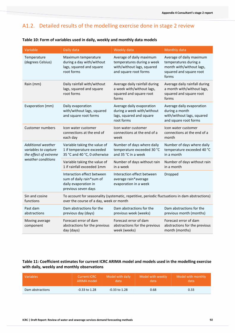
92
Appendix 4 Consultant’s stage 2 report
ICRC | Draft Report: Review of water and sewerage services demand forecasting methods
A1.2. Detailed results of the modelling exercise done in stage 2 review
Table 10: Form of variables used in daily, weekly and monthly data models
Variable Daily data Weekly data Monthly data
Temperature (degrees Celsius)
Maximum temperature during a day with/without lags, squared and square root forms
Average of daily maximum temperatures during a week with/without lags, squared and square root forms
Average of daily maximum temperatures during a month with/without lags, squared and square root forms
Rain (mm) Daily rainfall with/without lags, squared and square root forms
Average daily rainfall during a week with/without lags, squared and square root forms
Average daily rainfall during a month with/without lags, squared and square root forms
Evaporation (mm) Daily evaporation with/without lags, squared and square root forms
Average daily evaporation during a week with/without lags, squared and square root forms
Average daily evaporation during a month with/without lags, squared and square root forms
Customer numbers Icon water customer connections at the end of each day
Icon water customer connections at the end of a week
Icon water customer connections at the end of a month
Additional weather variables to capture the effect of extreme weather conditions
Variable taking the value of 1 if temperature exceeded 35 °C and 40 °C, 0 otherwise
Number of days where daily temperature exceeded 30 °C and 35 °C in a week
Number of days where daily temperature exceeded 40 °C in a month
Variable taking the value of 1 if rainfall exceeded 1mm
Number of days without rain in a week
Number of days without rain in a month
Interaction effect between sum of daily rain*sum of daily evaporation in previous seven days
Interaction effect between average rain*average evaporation in a week
Dropped
Sin and cosine functions
To account for seasonality (systematic, repetitive, periodic fluctuations in dam abstractions) over the course of a day, week or month
Past dam abstractions
Dam abstractions for the previous day (days)
Dam abstractions for the previous week (weeks)
Dam abstractions for the previous month (months)
Moving average component
Forecast error of dam abstractions for the previous day (days)
Forecast error of dam abstractions for the previous week (weeks)
Forecast error of dam abstractions for the previous month (months)
Table 11: Coefficient estimates for current ICRC ARIMA model and models used in the modelling exercise with daily, weekly and monthly observations
Variables Current ICRC ARIMA model
Model with daily data
Model with weekly data
Model with monthly data
Dam abstractions -0.33 to 1.28 -0.33 to 1.28 0.68 0.33
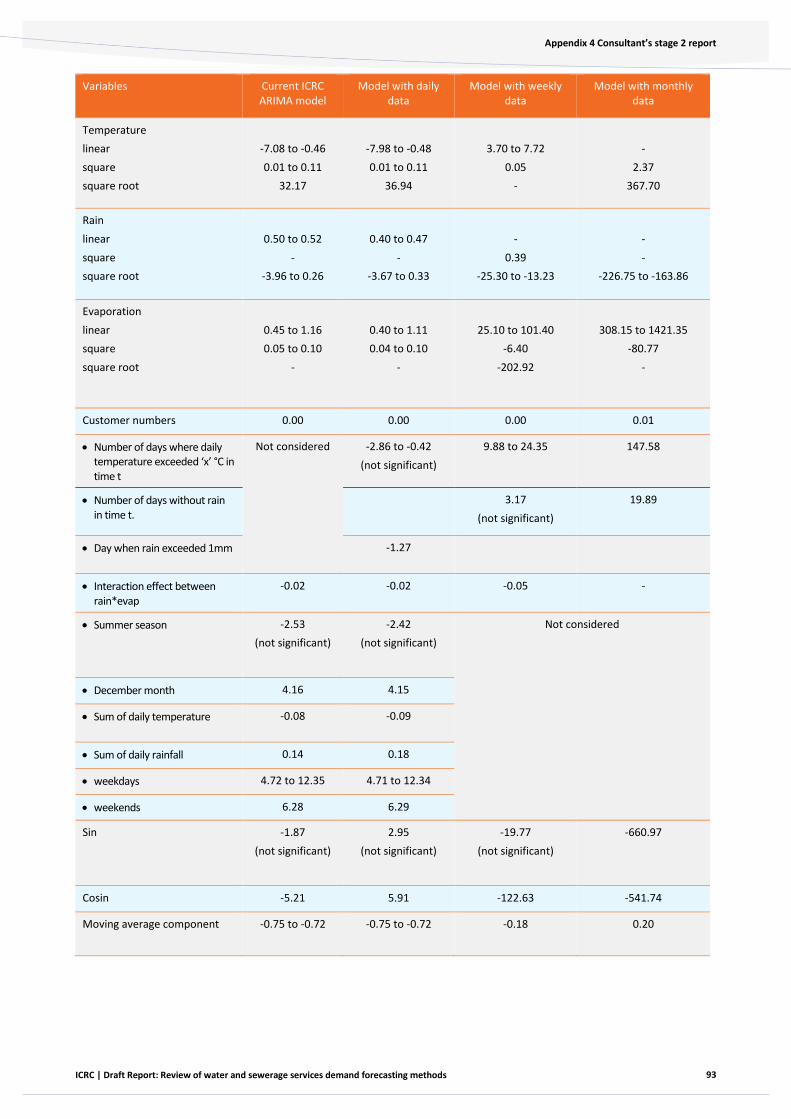
93
Appendix 4 Consultant’s stage 2 report
ICRC | Draft Report: Review of water and sewerage services demand forecasting methods
Variables Current ICRC ARIMA model
Model with daily data
Model with weekly data
Model with monthly data
Temperature
linear
square
square root
-7.08 to -0.46
0.01 to 0.11
32.17
-7.98 to -0.48
0.01 to 0.11
36.94
3.70 to 7.72
0.05
-
-
2.37
367.70
Rain
linear
square
square root
0.50 to 0.52
-
-3.96 to 0.26
0.40 to 0.47
-
-3.67 to 0.33
-
0.39
-25.30 to -13.23
-
-
-226.75 to -163.86
Evaporation
linear
square
square root
0.45 to 1.16
0.05 to 0.10
-
0.40 to 1.11
0.04 to 0.10
-
25.10 to 101.40
-6.40
-202.92
308.15 to 1421.35
-80.77
-
Customer numbers 0.00 0.00 0.00 0.01
• Number of days where daily temperature exceeded ‘x’ °C in time t
Not considered -2.86 to -0.42
(not significant)
9.88 to 24.35 147.58
• Number of days without rain in time t.
3.17
(not significant)
19.89
• Day when rain exceeded 1mm -1.27
• Interaction effect between rain*evap
-0.02 -0.02 -0.05 -
• Summer season -2.53
(not significant)
-2.42
(not significant)
Not considered
• December month 4.16 4.15
• Sum of daily temperature -0.08 -0.09
• Sum of daily rainfall 0.14 0.18
• weekdays 4.72 to 12.35 4.71 to 12.34
• weekends 6.28 6.29
Sin -1.87
(not significant)
2.95
(not significant)
-19.77
(not significant)
-660.97
Cosin -5.21 5.91 -122.63 -541.74
Moving average component -0.75 to -0.72 -0.75 to -0.72 -0.18 0.20

94
Appendix 4 Consultant’s stage 2 report
ICRC | Draft Report: Review of water and sewerage services demand forecasting methods
Note: coefficient estimate range is based on point estimates for different forms of a variable (squared, square root, lag, no lag) and
are considered for estimates that are statistically significant with a p-value of at most 0.05. To note the sign of the coefficient need
not necessarily be equal to what is expected when it comes to the sign of the coefficient for the linear component.
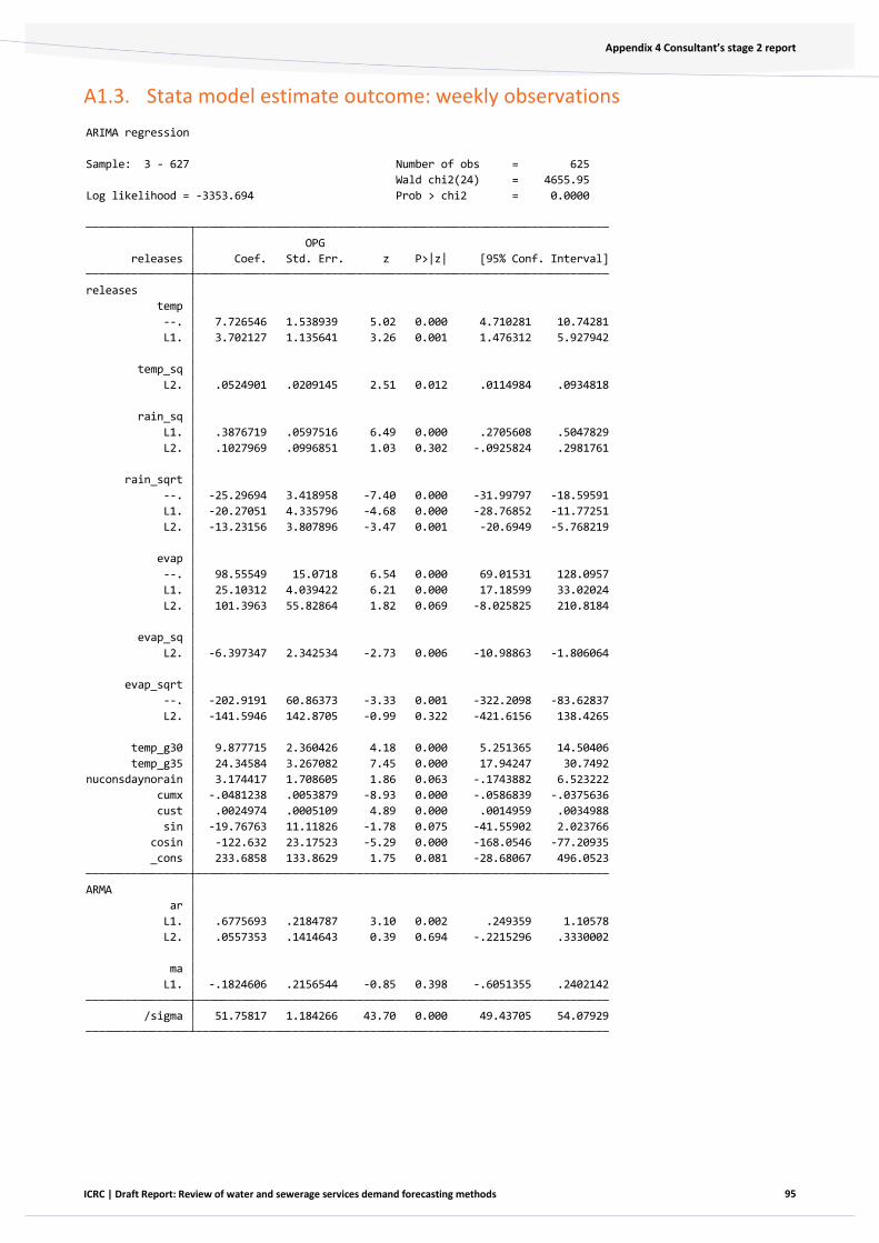
95
Appendix 4 Consultant’s stage 2 report
ICRC | Draft Report: Review of water and sewerage services demand forecasting methods
A1.3. Stata model estimate outcome: weekly observations
/sigma 51.75817 1.184266 43.70 0.000 49.43705 54.07929
L1. -.1824606 .2156544 -0.85 0.398 -.6051355 .2402142
ma
L2. .0557353 .1414643 0.39 0.694 -.2215296 .3330002
L1. .6775693 .2184787 3.10 0.002 .249359 1.10578
ar
ARMA
_cons 233.6858 133.8629 1.75 0.081 -28.68067 496.0523
cosin -122.632 23.17523 -5.29 0.000 -168.0546 -77.20935
sin -19.76763 11.11826 -1.78 0.075 -41.55902 2.023766
cust .0024974 .0005109 4.89 0.000 .0014959 .0034988
cumx -.0481238 .0053879 -8.93 0.000 -.0586839 -.0375636
nuconsdaynorain 3.174417 1.708605 1.86 0.063 -.1743882 6.523222
temp_g35 24.34584 3.267082 7.45 0.000 17.94247 30.7492
temp_g30 9.877715 2.360426 4.18 0.000 5.251365 14.50406
L2. -141.5946 142.8705 -0.99 0.322 -421.6156 138.4265
--. -202.9191 60.86373 -3.33 0.001 -322.2098 -83.62837
evap_sqrt
L2. -6.397347 2.342534 -2.73 0.006 -10.98863 -1.806064
evap_sq
L2. 101.3963 55.82864 1.82 0.069 -8.025825 210.8184
L1. 25.10312 4.039422 6.21 0.000 17.18599 33.02024
--. 98.55549 15.0718 6.54 0.000 69.01531 128.0957
evap
L2. -13.23156 3.807896 -3.47 0.001 -20.6949 -5.768219
L1. -20.27051 4.335796 -4.68 0.000 -28.76852 -11.77251
--. -25.29694 3.418958 -7.40 0.000 -31.99797 -18.59591
rain_sqrt
L2. .1027969 .0996851 1.03 0.302 -.0925824 .2981761
L1. .3876719 .0597516 6.49 0.000 .2705608 .5047829
rain_sq
L2. .0524901 .0209145 2.51 0.012 .0114984 .0934818
temp_sq
L1. 3.702127 1.135641 3.26 0.001 1.476312 5.927942
--. 7.726546 1.538939 5.02 0.000 4.710281 10.74281
temp
releases
releases Coef. Std. Err. z P>|z| [95% Conf. Interval]
OPG
Log likelihood = -3353.694 Prob > chi2 = 0.0000
Wald chi2(24) = 4655.95
Sample: 3 - 627 Number of obs = 625
ARIMA regression
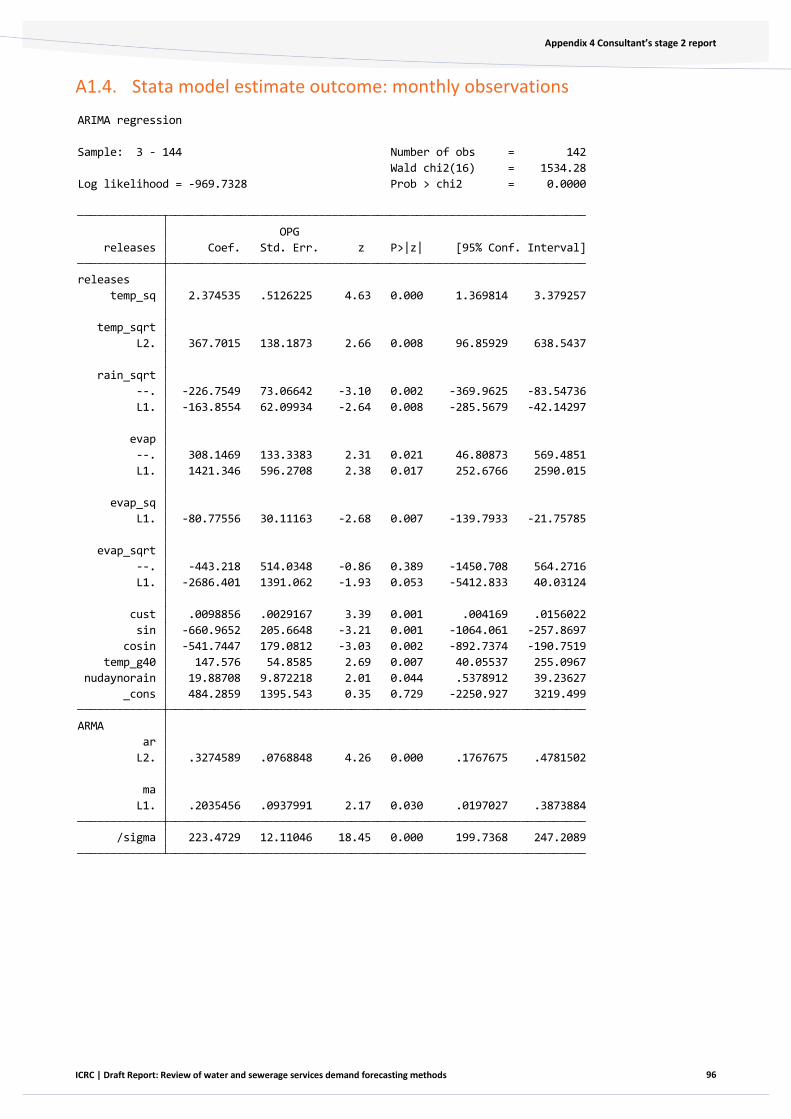
96
Appendix 4 Consultant’s stage 2 report
ICRC | Draft Report: Review of water and sewerage services demand forecasting methods
A1.4. Stata model estimate outcome: monthly observations
/sigma 223.4729 12.11046 18.45 0.000 199.7368 247.2089
L1. .2035456 .0937991 2.17 0.030 .0197027 .3873884
ma
L2. .3274589 .0768848 4.26 0.000 .1767675 .4781502
ar
ARMA
_cons 484.2859 1395.543 0.35 0.729 -2250.927 3219.499
nudaynorain 19.88708 9.872218 2.01 0.044 .5378912 39.23627
temp_g40 147.576 54.8585 2.69 0.007 40.05537 255.0967
cosin -541.7447 179.0812 -3.03 0.002 -892.7374 -190.7519
sin -660.9652 205.6648 -3.21 0.001 -1064.061 -257.8697
cust .0098856 .0029167 3.39 0.001 .004169 .0156022
L1. -2686.401 1391.062 -1.93 0.053 -5412.833 40.03124
--. -443.218 514.0348 -0.86 0.389 -1450.708 564.2716
evap_sqrt
L1. -80.77556 30.11163 -2.68 0.007 -139.7933 -21.75785
evap_sq
L1. 1421.346 596.2708 2.38 0.017 252.6766 2590.015
--. 308.1469 133.3383 2.31 0.021 46.80873 569.4851
evap
L1. -163.8554 62.09934 -2.64 0.008 -285.5679 -42.14297
--. -226.7549 73.06642 -3.10 0.002 -369.9625 -83.54736
rain_sqrt
L2. 367.7015 138.1873 2.66 0.008 96.85929 638.5437
temp_sqrt
temp_sq 2.374535 .5126225 4.63 0.000 1.369814 3.379257
releases
releases Coef. Std. Err. z P>|z| [95% Conf. Interval]
OPG
Log likelihood = -969.7328 Prob > chi2 = 0.0000
Wald chi2(16) = 1534.28
Sample: 3 - 144 Number of obs = 142
ARIMA regression

97
Appendix 4 Consultant’s stage 2 report
ICRC | Draft Report: Review of water and sewerage services demand forecasting methods
A1.5. Stata model estimate outcome: daily observations
/sigma 8.006017 .0623198 128.47 0.000 7.883872 8.128161
L1. -.7224889 .0284 -25.44 0.000 -.7781519 -.6668259
ma
L2. -.0338743 .0191715 -1.77 0.077 -.0714498 .0037013
L1. .9186684 .0323196 28.42 0.000 .8553232 .9820136
ar
ARMA7
L1. -.7551262 .0270915 -27.87 0.000 -.8082245 -.7020279
ma
L2. -.328319 .0247627 -13.26 0.000 -.376853 -.2797849
L1. 1.284877 .0304951 42.13 0.000 1.225107 1.344646
ar
ARMA
_cons 23.0336 31.62038 0.73 0.466 -38.9412 85.0084
nudaygeq1mm -1.273972 .3087555 -4.13 0.000 -1.879122 -.6688228
temp_g40 -2.863612 1.574092 -1.82 0.069 -5.948776 .221552
temp_g35 -.4244704 .8223144 -0.52 0.606 -2.036177 1.187236
cosin 5.911889 2.63163 2.25 0.025 .7539894 11.06979
sin 2.948543 2.19214 1.35 0.179 -1.347972 7.245059
cust .0003023 .0001502 2.01 0.044 7.94e-06 .0005966
summer -2.424963 1.444769 -1.68 0.093 -5.256658 .4067319
dec 4.151659 1.222934 3.39 0.001 1.754752 6.548566
fri 4.84134 1.024178 4.73 0.000 2.833988 6.848691
thu 4.706281 1.231608 3.82 0.000 2.292374 7.120188
wed 5.620609 1.272798 4.42 0.000 3.12597 8.115247
tue 6.74024 1.16149 5.80 0.000 4.46376 9.016719
mon 12.34155 1.078199 11.45 0.000 10.22832 14.45478
sun 6.292645 .9364672 6.72 0.000 4.457203 8.128087
cumrain .1859015 .0303734 6.12 0.000 .1263708 .2454323
cumtemp -.0871425 .021917 -3.98 0.000 -.1300991 -.044186
cumx -.0163333 .0010595 -15.42 0.000 -.0184099 -.0142567
L5. .0449269 .0092634 4.85 0.000 .0267711 .0630828
L1. .0715488 .0253517 2.82 0.005 .0218604 .1212373
--. .1014326 .025865 3.92 0.000 .0507381 .1521272
evap_sq
L4. .3933971 .1086623 3.62 0.000 .1804229 .6063714
L3. .8172342 .1023415 7.99 0.000 .6166484 1.01782
L2. 1.095693 .1005909 10.89 0.000 .8985384 1.292848
L1. .9407145 .2718417 3.46 0.001 .4079145 1.473515
--. 1.10556 .260575 4.24 0.000 .5948428 1.616278
evap
L8. -.4536439 .1178368 -3.85 0.000 -.6845998 -.2226879
L7. -.5825196 .1222904 -4.76 0.000 -.8222043 -.3428348
L6. .3292219 .1321639 2.49 0.013 .0701854 .5882585
L3. -.4226095 .1324597 -3.19 0.001 -.6822257 -.1629934
L1. -3.672695 .2841228 -12.93 0.000 -4.229565 -3.115824
--. -2.976194 .2744773 -10.84 0.000 -3.51416 -2.438229
rain_sqrt
L1. .4713036 .0575249 8.19 0.000 .3585568 .5840504
--. .4054549 .0569256 7.12 0.000 .2938828 .5170271
rain
L1. 36.94334 12.37749 2.98 0.003 12.6839 61.20278
temp_sqrt
L12. .0133237 .0034923 3.82 0.000 .0064789 .0201684
L5. .0057544 .0008746 6.58 0.000 .0040402 .0074686
L1. .1157031 .0156874 7.38 0.000 .0849562 .1464499
--. .0253145 .0036361 6.96 0.000 .0181879 .0324411
temp_sq
L12. -.4773042 .1857446 -2.57 0.010 -.8413569 -.1132514
L1. -7.981397 2.028009 -3.94 0.000 -11.95622 -4.006572
--. -.6514732 .1938243 -3.36 0.001 -1.031362 -.2715845
temp
releases
releases Coef. Std. Err. z P>|z| [95% Conf. Interval]
OPG
Log likelihood = -13700.56 Prob > chi2 = 0.0000
Wald chi2(47) = 112326.51
Sample: 12 - 3927, but with a gap Number of obs = 3915
ARIMA regression

98
Appendix 4 Consultant’s stage 2 report
ICRC | Draft Report: Review of water and sewerage services demand forecasting methods
Contact us
Rob Nolan Associate Director
0401947136
Marsden Jacob Associates Pty Ltd
03 8808 7400
Marsden Jacob Associates www.marsdenjacob.com.au
99
Appendix 5 Other Australian jurisdictions’ approaches to forecasting water demand
ICRC | Draft Report: Review of water and sewerage services demand forecasting methods
Appendix 5 Other Australian jurisdictions’ approaches to forecasting water demand
This appendix summarises the demand forecasting models used by water utilities in other jurisdictions. In developing this summary, we considered the reasoning behind the adopted approaches in these jurisdictions.
Each of the utilities reviewed here use the demand forecasting methodology that was most suited to the type of data they were readily able to access and how the demand forecasts were used.
In the case of Sydney Water and Hunter Water, which uses panel data regression and end use approaches respectively, demand forecasts are not only used as part of their regulatory determination for setting prices, but they are also used for water conservation reporting, which is required under IPART’s ELWC methodology. This explains their need for a flexible approach that considers additional factors than may be adequately provided under an ARIMA approach.
Melbourne Water contracts the bulk of its supply through three large customers, which in turn distribute water to the end user. As each of these customers does their own demand forecasting, Melbourne Water is able to make its demand forecasts based on the usage of its three largest customers.
SA Water uses an econometric model based on the historical water usage it has access to, and forecasts demand based on relationships observed between water demand and its drivers after the millennium drought.
SA Water
SA Water is regulated by the Essential Services Commission of Australia (ESCOSA), which uses a cost-based (building block) approach to determine a revenue cap for drinking water and sewerage services.
SA Water’s demand forecasting model was introduced in its 2013 Regulatory Business Proposal. SA Water developed the model to account for the increasingly volatile water demand (in the aftermath of the millennium drought) and considering that a growing share of SA Water’s revenue is derived from water sales led (SA Water 2013).
For the 2020-24 regulatory period, SA Water used an econometric regression model based on the relationship between annual bulk water usage, and climate (rainfall, evaporation and temperature) and population. Due to the seasonal pattern of water demand, SA Water’s water demand model also incorporates separate regression models for summer and winter (Acil Allen 2019).
SA Water uses the model for water planning and calculation of revenue and pricing for regulatory purposes. SA Water has access to water usage and other data extending back to the late 1992. However, in calibrating its demand model it chose not to use data collected before December 2010 when water restrictions were lifted and replaced with permanent water wise measures. Through a process of trial and error, the ‘best’ regression model is identified and used for forecasting from 2017-18 to 2023-24 (Acil Allen 2019).
Forecasts of bulk water usage per capita are produced for low, medium, average and high scenarios of climate. These climate scenarios are developed based on the climate patterns observed in the historical data. Monthly bulk water usage values are calculated by multiplying the per capita forecast by projected population figures using a 0.60 % annual growth rate. The monthly forecasts are then aggregated for

100
Appendix 5 Other Australian jurisdictions’ approaches to forecasting water demand
ICRC | Draft Report: Review of water and sewerage services demand forecasting methods
annual forecasts. Applying the non-revenue water proportion of 13.50% then provides the split of water demand into billed water and non-revenue water demands (Acil Allen 2019).
SA Water developed the demand forecasting model considering the following principles set out by ESCOSA that demand forecasts should:
• be free from statistical bias
• recognise and reflect key drivers of demand
• be based on sound assumptions using the best available information
• be consistent with other available forecasts and methodologies
• be based upon the most recently available data
• reflect the particular situation and the nature of the market for services
• be based upon sound and robust accounts of current market conditions and future prospects (SA Water 2013).
SA Water’s demand model applies a post-model adjustment to account for improvements to water efficiency. In arriving at its estimate of water efficiency, SA Water considered:
• the uptake of more water efficient products of toilets, washing machines and showerheads from its household appliance efficiency models for South Australia
• the changing household densities and housing types in South Australia (Acil Allen 2019).
SA Water’s analysis concluded that an efficiency per capita rate of 0.2 % per annum should be applied to the forecasts of the regression model (Acil Allen 2019).
We note the similarities in the demand drivers used by SA Water and those used in the ACT. The above information suggests that SA Water adopted an econometric modelling approach due to its flexibility to accommodate different climate scenarios and the availability of required data, given that SA Water intended to capture changes in consumer demand arising from drought related response measures.
Melbourne Water
Melbourne Water is regulated by the Essential Services Commission of Victoria (ESC), which implements a price cap form of price control. Melbourne Water uses an end use approach to determine observed water usage, using information provided by its three major customers: City West Water, South East Water and Yarra Valley Water (ESC 2021).
Melbourne Water forecasts bulk water demand based on forecasts provided by these retail water businesses (which use integrated-supply demand planning models to forecast demand). The inputs for the model are taken from periodic end use studies (ESC 2021). Key features of this modelling approach are:
• total demand estimate is a function of separate residential, non-residential water and non-revenue water forecasts
• efficiencies of appliance-based end uses and other parameters such as showering frequency and duration can be incorporated
• various calibration variables can be used such as residential water demand for outdoor water use, non-residential water demand and non-revenue water
• most recently completed end use studies are used.
Non-residential forecasts rely on bottom-up aggregation of historical demands and projections using observed trends or relationships. Non-revenue water forecasts rely on observed trends or relationships to factors and are adjusted for any future non-revenue water management activities.

101
Appendix 5 Other Australian jurisdictions’ approaches to forecasting water demand
ICRC | Draft Report: Review of water and sewerage services demand forecasting methods
Melbourne Water uses these end use data observations in conjunction with population projections and climate data to develop its demand forecasts. As the bulk of Melbourne Water’s demand is contracted through these three large customers, it makes sense for Melbourne Water to adopt an end use approach due to the relative ease it has in obtaining this data.
Sydney Water
Sydney Water is regulated by Independent Pricing and Regulatory Tribunal (IPART), which uses a building block approach to determine the notional revenue requirement for Sydney Water paired with demand forecasts to apply a price cap. Sydney Water uses a panel data regression approach to forecast water demand. Panel data regressions use repeated observations for the same customers over time to forecast demand.
Sydney Water uses a three-part approach for water demand forecasting:
1. It uses historical information to determine what factors influence water consumption. To do this, Sydney Water divides its customer base into 34 segments based on factors such as dwelling or business type, lot size and whether the property was built under the Building Sustainability Index21 system.
2. Sydney water then estimates an econometric panel data model for each segment based on historical customer usage. The parameters of this model capture the impact of the factors that influence water consumption within each group, such as price elasticity, weather, and seasonality on water demand.
3. Sydney Water then forecasts water demand by feeding in the forecast growth in customer numbers in each customer segment, climate projections, and estimates of system water losses and price elasticity to the econometric model (IPART 2020).
Sydney Water’s model forecast water demand based on average climate conditions because the model is not able to accurately predict climate conditions over the regulatory period (IPART 2020).
Sydney Water’s approach appears necessary for it to carry out its water conservation obligations under IPART’s Economic Level of Water Conservation methodology (ELWC). Under the ELWC, Sydney Water is required to submit (for IPART’s approval) reports outlining their approach to, and principles for, their methodology for determining their economic level of water conservation (Sydney Water 2019). This includes addressing the following elements of water conservation:
• Water leakage
• Water recycling
• Water efficiency (including demand management)
The ELWC methodology enables Sydney Water to adopt an approach to demand forecasting that allows them flexibility to forecast the data requirements specified above. We also note that dam abstraction data would be held by Water NSW and may not be something that Sydney Water has ready access to, whereas they do have ready access to end use customers.
Hunter Water
Hunter Water uses a supply demand planning model called the Integrated Supply-Demand Planning (iSDP) model to forecast water demand. Hunter Water’s iSDP model forecasts the water demand for average climate conditions. Unanticipated climate events such as drought or above average rainfall are not
—————
21 The Building Sustainability Index is a sustainability planning system in the NSW. Its requirements apply to all residential dwelling types in NSW and meeting its requirements is a part of the development application process.
102
Appendix 5 Other Australian jurisdictions’ approaches to forecasting water demand
ICRC | Draft Report: Review of water and sewerage services demand forecasting methods
considered in Hunter Water’s model. Therefore, these events can significantly affect the accuracy of forecasts.
The model uses demographic factors such as population growth, number of dwellings/connections and household size to forecast demand. Hunter Water updates demographic and connection numbers annually as part of its planning process.
The model forecasts water demand for residential customers and non-residential customers separately.
For residential customers, it forecasts demand based on expected water uses for various activities such as residential toilets, showers, taps, washing machines and gardens. The iSDP model has separate model modules to calculate demand for each activity. These modules forecast demand based on detailed information on installed equipment and the frequency of use. Hunter Water has access to annual sales data for individual appliances which it uses as an input to the model. In some cases, Hunter Water estimates the sales using data on appliance ownership in each year in combination with assumptions about the duration of time that appliances remain in service prior to being replaced.
For non-residential customers, it uses a trend analysis to forecast the demand. Hunter Water uses economic trends, changes in recycled water demand and water conservation measures as inputs to the model.
The model calculates non-revenue water using Water Services Association of Australia national reporting methodology.
Like Sydney Water, Hunter Water is subject to IPART’s ELWC methodology and therefore requires a more flexible approach than ARIMA to facilitate the forecasting of variables required to meet requirements (Hunter Water 2020).
ACT – Icon Water
In 2015, we released a technical paper outlining the ARIMA approach to forecast water demand. We considered that the approach then used—Cardno’s approach to forecast water usage per customer based on annual observations for water users separated into four subgroups—was insufficient (ICRC 2015b). We found that Cardno’s approach:
• restricted data availability, as it relied on 13 annual observations
• did not consider the effect of the millennium drought on changing water consumption behaviour of consumers.
We considered that Cardno’s approach overstated demand for water given that it did not account for the step-change in demand from the millennium drought and that this created a risk that Icon Water would not be able to recover its efficient costs due to the lower prices that would have eventuated from overstated forecast demand.
In comparison, we found in 2015 that data on water abstractions from Icon Water’s dams was readily available. We found there was a stable and direct relationship between dam abstractions and ACT water sales and considered dam abstractions was a good indicator of water demand by ACT consumers. We also required dam abstractions forecast to assess Icon Water’s operating and capital costs and the water abstraction charge. We found ARIMA approach was better suited to model dam abstractions, because data are available at a high frequency for a long time period (ICRC 2015).

103
0 Abbreviations and acronyms
ICRC | Draft Report: Review of water and sewerage services demand forecasting methods
Abbreviations and acronyms
ABS Australian Bureau of Statistics
ACCESS-S Australian Community Climate and Earth System Simulator -Seasonal
ACT Australian Capital Territory
AER Australian Energy Regulator
AIC Akaike Information Criteria
ARIMA Autoregressive Integrated Moving Average
BoM Bureau of Meteorology
EEIS Energy Efficiency Improvement Scheme
ELWC Economic Level of Water Conservation
ENSO El Nino-Southern Oscillation
ESC Essential Services Commission of Victoria
ESCOSA Essential Services Commission of South Australia
GCM Global climate model
GL Gigalitre
ICRC Independent Competition and Regulatory Commission
IOD Indian Ocean Dipole
IPART Independent Pricing and Regulatory Tribunal
iSDP Integrated Supply-Demand Planning
kL kilolitres
MAPE Mean Absolute Percent Error
MDBA Murray-Darling Basin Authority
ML Megalitres
NARCLiM NSW and ACT Regional Climate Modelling
NSW New South Wales
RCM Regional Climate Model

104
0 Abbreviations and acronyms
ICRC | Draft Report: Review of water and sewerage services demand forecasting methods
RCP Representation Concentration Pathways
RMSPE Root Mean Square Percentage Error
SA South Australia
SDL Sustainable diversion limit
SEACI South Eastern Australian Climate Initiative
105
0 References
ICRC | Draft Report: Review of water and sewerage services demand forecasting methods
References
Acil Allen (Acil Allen Consulting) (2019) ‘ACIL Allen Demand model audit’, Water Demand Model Review, Acil Allen.
ACT Government (Australian Capital Territory Government) (2019) ACT Population Projections 2018 to 2058, ACT Government.
ACT Government (Australian Capital Territory Government) (2021) ACT 2020–21 Budget Outlook.
AER (Australian Energy Regulator) (2021) Final Decision Evoenergy Access Arrangement 2021 to 2026 Overview, AER, Australian Government.
EPSDD (Environment, Planning and Sustainable Development Directorate) (2019) ACT Water Resource Plan, EPSDD.
ESC (Essential Services Commission) (2021) Melbourne Water Final Decision, ESC, Victorian Government.
ESCOSA (Essential Services Commission of South Australia) (2013) SA Water’s Water and Sewerage Revenues 2013/14 – 2015/16 – Draft determination: Statement of reasons, ESCOSA.
Hunter Water (2020) Water Conservation Report, Hunter Water.
Icon Water (2017) ‘Attachment 4 Demand forecasts’, 2018–23 Water and Sewerage Price Proposal, Icon Water.
Icon Water (2018) Submission to draft decision, Icon Water.
Icon Water (2021) Review of water and sewerage services demand forecasting methodology: Icon Water submission to ICRC Issues Paper, Icon Water.
ICRC (Independent Competition and Regulatory Commission) (2015) Water demand forecasting: Final technical paper, ICRC.
ICRC (Independent Competition and Regulatory Commission) (2015b) Regulated water and sewerage services - The Industry Panel process: Outcomes and prospects, ICRC.
ICRC (Independent Competition and Regulatory Commission) (2017a) Final report Tariff structure review 2016-17, ICRC.
ICRC (Independent Competition and Regulatory Commission) (2017b) Icon Water Price Proposal 2018–23 - Attachments, Attachment 4, ICRC, accessed 06 September 2021.
ICRC (Independent Competition and Regulatory Commission) (2018) Regulated water and sewerage services prices 2018–23, ICRC.
ICRC (Independent Competition and Regulatory Commission) (2020a) Consumer Protection Code 2020, ICRC.
ICRC (Independent Competition and Regulatory Commission) (2020b) Water and Sewerage Services Price Regulation: Incentive Mechanisms, ICRC.
IPART (Independent Pricing and Regulatory Tribunal) (2020) Final report on prices for Sydney Water, IPART.

106
0 References
ICRC | Draft Report: Review of water and sewerage services demand forecasting methods
Marsden Jacob Associates (2021a) Water demand forecasting methodology review – Stage 1 report, Marsden Jacob.
Marsden Jacob Associates (2021b) Water demand forecasting methodology review – Stage 2 report, Marsden Jacob.
Professor Ian White (2021), Submission to: ICRC Review of Water and Sewerage Demand Forecasting Methods: Frequency of Droughts and ICON Water’s ±6% Demand ‘Deadband’, Ian White.
SA Water (South Australia Water Corporation) (2013) Regulatory Business Proposal 2013, SA Water, Government of South Australia.
Sydney Water (2019) Determining Sydney Water’s Economic Level of Water Conservation, Sydney Water.

www.icrc.act.gov.au


