
Journal of Applied and Industrial Sciences, 2014, 2 (1): 35-45, ISSN: 2328-4595 (PRINT), ISSN: 2328-4609 (ONLINE)
Research Article 35
Abstract-Two control strategies were undertaken for the system
water-Acetic acid- normal hexane in a rotating disc contactor
(R.D.C).The first cascade control system consists of a raffinate
composition variable transmitted to the primary controller that
transmits it’s output as the set point to the level controller of the
secondary loop. The second strategy takes the extract composition
transmitted to the primary controller which transmits its output
to the secondary level controller. The transfer functions for both
primary and secondary loops were identified, the overall transfer
functions were calculated for both primary and secondary loops
and consequently tuned by Routh, root locus and Bode methods.
The adjustable parameters for primary and secondary loops Kc’s ,
τi’s, τd’s were determined and optimized by Ziegler-Nichols
method. The offsets were determined and it was found that they
were reasonable for the secondary loop, but considerably high for
the primary loop. Therefore the gain Kc1 of the primary loop was
refined by trial and error to 3.5. This increase in the primary gain
reduced the offset to (- 0.239) which is a reasonable value and the
primary parameters were adjusted accordingly. The response of
each method of tuning was plotted and the characteristics of the
close loop responses were compared and found to be in agreement
as shown in figures 7,8,9,10,11,12,13,14,15,16,17,18.
Index Terms-Cascade control, Tuning, Offset, Responses
investigation.
I. INTRODUCTION
iquid-liquid extraction is a process that separates
components based upon solubility in solvents. The
liquid-liquid extraction is termed as solvent extraction,
extraction, or liquid extraction. The basic principle behind
extraction involves the contacting of a solution with another
solvent which is immiscible with the original; the solvent is
also soluble with specific solute contained in the solution. Two
phases are formed after the addition of the solvent, due to the
differences in densities. The solvent is chosen, so that the solute
in solution has more affinity toward the added solvent,
therefore mass transfer of the solute from the solution to the
solvent occurs, further separation of the extracted solute and the
solvent will be necessary. [1] The control of these units can
often be problematic, partially due to their multiphase nature,
and partially due to the difficulty of on-line measurements of
output variables. Thus, the reliable simulation of the transient
behaviour of these columns is extremely valuable. The column
hydrodynamics including flooding, entrainment, weeping, and
phase inversion will be controlled. [1]
Routh Criterion
The Routh criterion determines the number of the roots of the
characteristic equation that lie on the left-half plane, the right
-half plane or on the imaginary axis if the system is stable,
unstable or critically stable respectively.
The Root Locus Method
This method gives an approximate graphical representation of
the root as the gain is varied. This is very useful in the design of
a system since it gives the position of the poles of the system in
the S-plane for all values of the gain [ 2 and 3].
Bode plot
Bode plot is the graph on semi log paper of the amplitude ratio
and phase angle as the frequency is varied from zero to infinity.
From the plot the ultimate gain and period can be determined
and used for tuning[2-5].
Control systems with multiple loops
The feedback control configuration involves one measurement
(output) and one manipulated variable in a single loop. There
are other simple control configurations which may be used. If
there are more than one measurement and one manipulated
variable or one measurement and more than one manipulated
variables in such case the control systems with multiple loops
may arise, typical example is the cascade control. [6 and 7]
Cascade control
In a cascade control configuration one manipulated variable
and more than one measurement exist.
Industrial Controllers
These are a combination of two or three modes together. They
are usually in actions of P, PI and PID. [1, 2]
Tuning of a Cascade Control System in a Rotating Disk
Contactor (RDC) H.A. Khalil
*1, G .A. Gasmelseed
2, A.E Elhassan
3
(1, 2, 3)Department of Chemical Engineering, Faculty of Engineering, University of Science and Technology
Email:[email protected]
Telephone: +249919634134
Email:[email protected]
Telephone: +249999773300
(Received: December 10, 2013; Accepted: February 04, 2014)
L
*Corresponding author Email:[email protected]
Telephone: +249123896466

Journal of Applied and Industrial Sciences, 2014, 2 (1): 35-45, ISSN: 2328-4595 (PRINT), ISSN: 2328-4609 (ONLINE)
Objectives
1. To develop a control strategy of liquid-liquid extraction
process.
2. To identify the transfer functions.
3. To investigate the tuning stability analysis and response
simulation.
II. MATERIALS AND METHODS
Control strategy
This is based on paring the controlled variables with
the manipulated variables; these were specified first
as shown in Fig. 1 and Fig. 2.
Figure 1: Physical diagram of strategy1
36
Figure 2: Physical diagram of strategy 2
From the loops specified in the control strategy the
block diagrams were drawn as shown in Fig. 3 and
Fig. 4.
Figure 3: General block diagram of cascade systems
L.T
C.T.
T L.c
C.C
Extract Feed
PS.
PS.
organic phase Raffinate
L.T
C.C
C.T L.C
FeedExtract
PS.
PS.
Gm2
Gc1
Gm1
Gp2
Gc2
Gv Gp1
- -

Journal of Applied and Industrial Sciences, 2014, 2 (1): 35-45, ISSN: 2328-4595 (PRINT), ISSN: 2328-4609 (ONLINE)
37
Figure 4: General reduced block diagram of the cascade system
Figure 5: The response by each criterion
Procedure for stability analysis and tuning
The appropriate transfer functions were cited [4].
The overall transfer functions were determined and
the open loop and close loop characteristic equations
were derived.
The characteristic equations developed in the
previous step were used for tuning, stability analysis
and offset investigation.
The response by each criterion were graphically
determined and compared for the best performance
with regard to overshoot, decay ratio, rise time and
recovery time (Fig. 5).
1- Over shoot :
=A=
√
2- Decay ratio :
= =
√
3- Rise time: the time required for the
response to first reach its ultimate value.
4- Response time: TR: settling time or recovery
time, time for the response to be within
of its ultimate value, sec.
5- Period of oscillation, T : time for complete
cycle, in sec.
√
, frequency in rad/s
√ in seconds
The inner loop (Secondary loop)
G(s) =
Πf = Gc2 Gv Gp2 1+ ΠL = 1+ Gc2 Gv Gp2 Gm2
G(s) =
The characteristic equation of the inner loop:-
1 + Gc2 Gv Gp2 Gm2 = 0
III. RESULTS AND DISCUSSION
The responses for secondary loop are:-
Proportional controller (P controller)
1- Routh (Fig. 6)
Kc=11.9
Gc1
Gm1
Gp1
+
- y(t)
C(t)
Rt0
A
B
±5%
C
rt response
time sec,,t
T)(tC

Journal of Applied and Industrial Sciences, 2014, 2 (1): 35-45, ISSN: 2328-4595 (PRINT), ISSN: 2328-4609 (ONLINE)
Step Response
Time (sec)
Am
plitu
de
0 50 100 150 200 2500
0.5
1
1.5
2
2.5
Step Response
Time (sec)
Am
plitu
de
0 50 100 150 200 2500
0.5
1
1.5
2
2.5
Figure 6: The responses for secondary loop for Proportional controller using Routh criteria
2- Root locus (Fig. 7) Kc=11.8
Figure 7: The responses for secondary loop for Proportional controller using Root locus

Journal of Applied and Industrial Sciences, 2014, 2 (1): 35-45, ISSN: 2328-4595 (PRINT), ISSN: 2328-4609 (ONLINE)
Step Response
Time (sec)
Ampl
itude
0 50 100 150 200 2500
0.5
1
1.5
2
2.5
0 50 100 150 200 250 300 350 400 450-0.5
0
0.5
1
1.5
2
2.5
Step Response
Time (sec)
Am
plitu
de
3- Bode plot (Fig. 8)
39
Kc=12.07
Figure 8: The responses for secondary loop for Proportional controller using Bode plot
Proportional integral controller (PI)
1- Routh (Fig. 9)
Kc=10.71 ,τi=33.139
Figure 9: The responses for secondary loop for Proportional integral controller using Routh criteria
Journal of Applied and Industrial Sciences, 2014, 2 (1): 35-45, ISSN: 2328-4595 (PRINT), ISSN: 2328-4609 (ONLINE)
0 100 200 300 400 500 600 700-0.5
0
0.5
1
1.5
2
2.5
Step Response
Time (sec)
Am
plit
ude
0 100 200 300 400 500 600 700 800-0.5
0
0.5
1
1.5
2
2.5
3
Step Response
Time (sec)
Ampli
tude
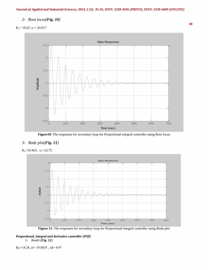
2- Root locus(Fig. 10) 40
Kc= 10.62 ,τi = 24.017
Figure10: The responses for secondary loop for Proportional integral controller using Root locus
3- Bode plot(Fig. 11)
Kc=10.863, τi= 23.75
Figure 11: The responses for secondary loop for Proportional integral controller using Bode plot
Proportional, integral and derivative controller (PID)
1- Routh (Fig. 12)
Kc=14.28 ,τi= 19.8835 , τd= 4.97

Journal of Applied and Industrial Sciences, 2014, 2 (1): 35-45, ISSN: 2328-4595 (PRINT), ISSN: 2328-4609 (ONLINE)
Step Response
Time (sec)
Ampl
itude
0 10 20 30 40 50 600
0.5
1
1.5
2
2.5
Step Response
Time (sec)
Am
plitu
de
0 50 100 1500
0.5
1
1.5
2
2.5
41
Figure 12: The responses for secondary loop for Proportional integral and derivative controller using Routh criteria
2- Root locus (Fig. 13)
Kc=14.16 ,τi=14.41 ,τid=3.6025
Figure 13: The responses for secondary loop for Proportional integral and derivative controller using Root locus
3- Bode plot ((Fig. 14)
Kc=14.484, τi= 14.25 , τid= 3.5625

Journal of Applied and Industrial Sciences, 2014, 2 (1): 35-45, ISSN: 2328-4595 (PRINT), ISSN: 2328-4609 (ONLINE)
Step Response
Time (sec)
Am
plitu
de
0 50 100 1500
0.5
1
1.5
2
2.5
Step Response
Time (sec)
Ampl
itude
0 0.1 0.2 0.3 0.4 0.5 0.60
0.1
0.2
0.3
0.4
0.5
0.6
0.7
0.8
0.9
1
System: G2
Final Value: 0.993System: G2
Settling Time (sec): 0.387System: G2
Rise Time (sec): 0.218
42
Figure 14: The responses for secondary loop for Proportional integral and derivative controller using Bode plot
For the second strategy:
The responses for secondary loop are:
Proportional Controller (P-Controller Only)
Kc=376.25 (Routh ) (Fig. 15)
Figure 15: The responses for secondary loop for Proportional controller using Routh criteria
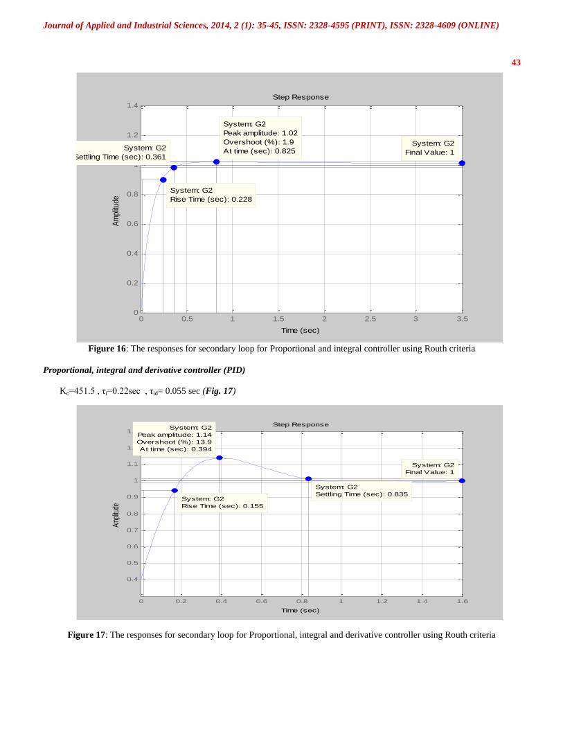
Proportional integral controller (PI)
Kc= 338.625, τi=3.68 sec (Fig. 16)
Journal of Applied and Industrial Sciences, 2014, 2 (1): 35-45, ISSN: 2328-4595 (PRINT), ISSN: 2328-4609 (ONLINE)
Step Response
Time (sec)
Am
plitu
de
0 0.5 1 1.5 2 2.5 3 3.50
0.2
0.4
0.6
0.8
1
1.2
1.4
System: G2
Final Value: 1
System: G2
Peak amplitude: 1.02
Overshoot (%): 1.9
At time (sec): 0.825System: G2
Settling Time (sec): 0.361
System: G2
Rise Time (sec): 0.228
Step Response
Time (sec)
Ampl
itude
0 0.2 0.4 0.6 0.8 1 1.2 1.4 1.6
0.4
0.5
0.6
0.7
0.8
0.9
1
1.1
1.2
1.3
System: G2
Final Value: 1
System: G2
Settling Time (sec): 0.835
System: G2
Peak amplitude: 1.14
Overshoot (%): 13.9
At time (sec): 0.394
System: G2
Rise Time (sec): 0.155
43
Figure 16: The responses for secondary loop for Proportional and integral controller using Routh criteria
Proportional, integral and derivative controller (PID)
Kc=451.5 , τi=0.22sec , τid= 0.055 sec (Fig. 17)
Figure 17: The responses for secondary loop for Proportional, integral and derivative controller using Routh criteria

Journal of Applied and Industrial Sciences, 2014, 2 (1): 35-45, ISSN: 2328-4595 (PRINT), ISSN: 2328-4609 (ONLINE)
Table 1 44
Comparison between the characteristic of the closed-loop responses using Different techniques for the secondary loop
Method Routh Root locus Bode plot
Type of
control
P PI PID P PI PID P PI PID
Kc 11.9 10.71 14.28 11.8 10.62 14.16 0.42385 0.381465 0.50862
τI(sec) ---- 33.139 19.8835 ---- 24.017 14.41 ---- 23.5855 14.1513
τD(sec) ---- ----- 4.97 ---- ---- 3.6025 ---- ------- 3.5378
overshoot 1.26 1.34 1.08 1.25 1.49 1.28 1.28 1.52 1.28
offset 0.05 0 0 0.01 0 0.005 0 0
Tr 3.91 4.26 1.49 3.93 4.24 1.99 3.87 4.17 1.96
Settling
timeTS
171 288 46.3 171 457 91.8 171 513 91.2
Period of
oscillation
38.1 40.5 17.01 38.7 40.7 38.8 38.2 40.9 38.49
Table 2
Comparison between the characteristic of the closed-loop responses using Different techniques for the primary loop
Method Routh Root locus Bode plot
Type of control P PI PID P PI PID P PI PID
Kc 0.9265 0.83385 1.1118 0.885 0.7965 1.062 0.42385 0.381465 0.50862
τI(sec) ---- 23.799 14.25 ---- 9.45125 5.67075 ---- 23.5855 14.1513
τD(sec) ---- ----- 3.56 ---- ---- 1.41768 ----- ----- 3.5378
overshoot 1.17 1.26 0.536 1.06 1.07 1.25 1.11 1.37 0.715
offset 0.009 0.005 0.003 0.005 0.001 0 0.001 0.001 0.002
Tr 1.9 2.94 1.78 2.98 3.05 2.4 3.4 3.42 2.21
Settling timeTR 220 82.1 23.8 457 59.5 97.7 83.9 136 >35
Period of
oscillation(Ps)
(sec)
11.69 22.9 24.02 21.94 22.9 21.69 28.4 30.1 19.11
A system of normal hexane- water – acetic acid – is
investigated with regard to controlling the efficiency of
separation and column hydrodynamics. A rotating Disc
Contactor column is used for a counter-current liquid-liquid
extraction of the above system.
A control strategy was developed using multi-loop cascade
control. In this study two strategies were undertaken. One
strategy takes the composition controller as a master controller
which transmits its output signal as a set point to the level slave
controller, which controls the input flow rate of the organic
phase as shown in figure 1. The second strategy uses the
composition controller of the extract that transmits its output
signal to the level secondary controller, in order to adjust the
feed rate as shown in figure 2.
The transfer function of each loop in each strategy were
identified and used to get the overall transfer functions and
characteristic equations. These transfer functions were use
through the method of Routh, Root locus and Bode plot to
determine the adjustable parameters (Kc , τi , τd) and the simple
performance parameters , overshoot, offset , settling time, Rise
time and period of oscillation.
These adjustable parameters were used to draw the response
using P,PI and PID controllers and it was found that the
responses give different performance as shown in figures
(6,7,8,9,10,11,12,13,14,15,16,17) and as stated in tables 1 and
2.
IV. CONCLUSIONS
It is concluded that cascade control tuning requires tuning the
secondary and primary loops separately, the adjustable
parameters calculated for the two loops are found to be
different and are not able to give a stable system when set to be
equal for both loops.
The method is to calculate the ultimate gain and ultimate period
for the secondary loop first and then calculating the same for
the primary loop and that the loop should be tuned separately.
ACKNOWLEDGEMENT
The authors wish to thank the College of Graduate Studies and
Scientific Research, Karary University for their help and
assistance to allow this partial research to accomplish. The
authors also wish to thank the technical staff of university of
Science and Technology, faculty of engineering-department of
chemical engineering for their help and permission to carry out
the experimental work.
REFERENCES [1]. http://vienna.che.uic.edu/teaching/che396/sepProj/Snrtem~1.pdf [2]. Seader,(1998). Principle of separation process –J. W,(I.N.C)-liquid-Liquid
extraction with ternary systems. pp ,419-449.
[3]. http://en.wikipedia.org/wiki/Concentration Last modified February 2008
[4]. Dale,E,Edgar, T.F and Duncan, A.M (1998). “Process Dynamic and
control. John Willey and Sons, New York.
[5]. Luyben, L.L (2007).” Process Modeling Simulation and Control for
chemical Engineering”. Mc Graw Hill Publishing Company, New York.

Journal of Applied and Industrial Sciences, 2014, 2 (1): 35-45, ISSN: 2328-4595 (PRINT), ISSN: 2328-4609 (ONLINE)
6]. Stephan Opoulus, G (1994). “Chemical process control An Introduction to Theory and Practice” Prentice Hall, India,.
45
[7]. Abu-Guok, M. E (2003). “Controlling Techniques and System Stability, University of Khartoum Press.


