arX
iv:c
ond-
mat
/000
9219
v1 1
4 Se
p 20
00
Renormalization Group and Probability Theory
G. Jona-Lasinio
Dipartimento di Fisica, Universita ”La Sapienza”
Piazzale A. Moro 2, 00185 ROMA, Italy
Abstract
The renormalization group has played an important role in the physics of
the second half of the twentieth century both as a conceptual and a calcula-
tional tool. In particular it provided the key ideas for the construction of a
qualitative and quantitative theory of the critical point in phase transitions
and started a new era in statistical mechanics. Probability theory lies at the
foundation of this branch of physics and the renormalization group has an
interesting probabilistic interpretation as it was recognized in the middle sev-
enties. This paper intends to provide a concise introduction to this aspect of
the theory of phase transitions which clarifies the deep statistical significance
of critical universality.
Typeset using REVTEX
1
Contents
I Introduction 2
II A Renormalization Group derivation of the Central Limit Theorem 6
III Hierarchical Models 8
IV Eigenvalues of the linearized RG and critical indices 11
V Self Similar Random Fields 13
VI Some Properties of Self Similar Random Fields 16
VII Multiplicative Structure 17
VIII RG and Effective Potentials 19
IX Coexistence of Phases in Hierarchical Models 21
X Weak perturbations of Gaussian measures:
a non Gaussian fixed point 23
XI Concluding Remarks 26
I. INTRODUCTION
The renormalization group (RG) is both a way of thinking and a calculational tool
which acquired its full maturity in connection with the theory of the critical point in phase
transitions. The basic physical idea of the RG is that when we deal with systems with
infinitely many degrees of freedom, like thermodynamic systems, there are relatively simple
relationships between properties at different space scales so that in many cases we are able
to write down explicit exact or approximate equations which allow us to study asymptotic
behaviour at very large scales.
2
The first systematic use of probabilistic methods in statistical mechanics was made by
Khinchin who showed, using the central limit theorem, that the Boltzmann distribution
of the single-molecule energy in systems of weakly correlated molecules is universal, that
is independent of the form of the interaction, provided it is of short range. In his well
known book [1] he emphasizes that physicists had not fully appreciated the generality of
probabilistic methods so that, for example, they provided a new derivation (usually heuristic)
of the Boltzmann law for every type of interaction. Similar remarks apply to the first
applications of the RG in statistical mechanics. RG was introduced as a tool to explain
theoretically the universality phenomena, the scaling laws, discovered experimentally near
the critical point of a phase transition. In the first period RG calculations used different
formal devices, mostly borrowed from quantum field theory, which gave good qualitative and
quantitative results. It was soon realized that a new class of limit theorems in probability
was involved. This class referred to situations of strongly correlated variables to which the
central limit theorem does not apply, that is situations opposite to those considered by
Khinchin. In fact, it was discovered that a critical point can be characterized by deviations
from the central limit theorem.
Before providing a description of the content of the present paper we give a short account
of the development of RG ideas in statistical mechanics.
It is useful to distinguish two different conceptual approaches. The first use of the RG in
the study of critical phenomena [2] was based on a Green’s function approach to statistical
mechanics which paralleled quantum field theory. We recall Eq. (1) of [2]
G(x, {yi}, α) = Z(t, {yi}, α) G(x/t, {yi/t}, αZ−1V (t, {yi}, α)Z2(t, {yi}, α)), (1.1)
where G is a dimensionless two-point Green function depending on a momentum variable
x, a set of physical parameters yi and the intensity of the interaction α (all dimensionless).
This is an exact generalized scaling relation which in the vicinity of the critical point reduces
to the phenomenological scaling due to the disappearance of the irrelevant parameters. The
scaling functions Z and ZV can be expressed in terms of the Green’s functions themselves
3
via certain normalization conditions. This equation provided a qualitative explanation of
scaling and, after the introduction of a non integer space dimension d and the use of ǫ = 4−d
as a perturbation parameter [3], became the basis for systematic quantitative calculations
[4], [5], [6].
The second approach started with the use on the part of Wilson of a different notion of
RG [7] that he had already introduced in a different context, the fixed source meson theory
[8], [9], with no reference to critical phenomena. This was akin to certain intuitive ideas
of Kadanoff [10] about the mechanism of reduction of relevant degrees of freedom near the
critical point. Kadanoff’s idea was that in the critical regime a thermodynamic system, due
to the strong correlations among the microscopic variables, behaves as if constituted by rigid
blocks of arbitrary size. In Wilson’s approach in fact the calculation of a statistical sum
consisted in a progressive elimination of the microscopic degrees of freedom to obtain the
asymptotic large scale properties of the system.
Formally the Green’s function and the Wilson method were very different and in partic-
ular the first one implied a true group structure while the second was a semigroup. Both
gave exactly the same results and the problem arose of clarifying the conceptual structures
underlying these methods. In fact many people were confused by this situation and some
thought that the two methods had little connection with each other. Actually the possibility
of different RG transformations equally effective in the study of critical properties could be
easily understood using concepts from the theory of dynamical systems. The critical point
corresponds to a fixed point of these transformations and the quantities of physical interest,
i.e. the critical indices, are connected with the hyperbolic behaviour in its neighborhood,
which is preserved if the different transformations are related by a differentiable map [11].
Still the multiplicative structure of the Green’s function RG and the elimination of degrees
of freedom typical of Wilson’s approach did not appear easy to reconcile. The formal connec-
tion was clarified in [12] where it was shown that to any type of RG transformation one can
associate a multiplicative structure, a cocycle, and the characterizing feature of the Green’s
function RG is that it is defined directly in terms of this structure. In the probabilistic
4
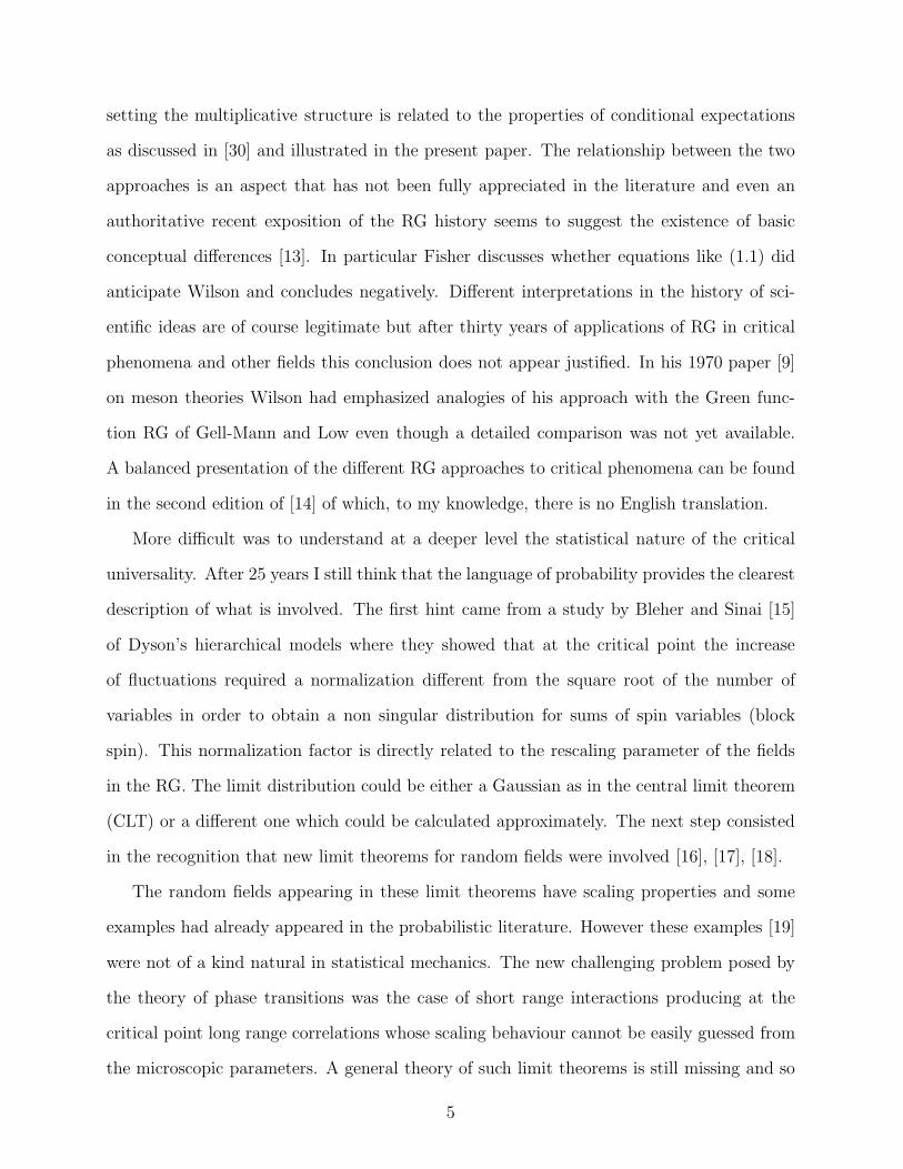
setting the multiplicative structure is related to the properties of conditional expectations
as discussed in [30] and illustrated in the present paper. The relationship between the two
approaches is an aspect that has not been fully appreciated in the literature and even an
authoritative recent exposition of the RG history seems to suggest the existence of basic
conceptual differences [13]. In particular Fisher discusses whether equations like (1.1) did
anticipate Wilson and concludes negatively. Different interpretations in the history of sci-
entific ideas are of course legitimate but after thirty years of applications of RG in critical
phenomena and other fields this conclusion does not appear justified. In his 1970 paper [9]
on meson theories Wilson had emphasized analogies of his approach with the Green func-
tion RG of Gell-Mann and Low even though a detailed comparison was not yet available.
A balanced presentation of the different RG approaches to critical phenomena can be found
in the second edition of [14] of which, to my knowledge, there is no English translation.
More difficult was to understand at a deeper level the statistical nature of the critical
universality. After 25 years I still think that the language of probability provides the clearest
description of what is involved. The first hint came from a study by Bleher and Sinai [15]
of Dyson’s hierarchical models where they showed that at the critical point the increase
of fluctuations required a normalization different from the square root of the number of
variables in order to obtain a non singular distribution for sums of spin variables (block
spin). This normalization factor is directly related to the rescaling parameter of the fields
in the RG. The limit distribution could be either a Gaussian as in the central limit theorem
(CLT) or a different one which could be calculated approximately. The next step consisted
in the recognition that new limit theorems for random fields were involved [16], [17], [18].
The random fields appearing in these limit theorems have scaling properties and some
examples had already appeared in the probabilistic literature. However these examples [19]
were not of a kind natural in statistical mechanics. The new challenging problem posed by
the theory of phase transitions was the case of short range interactions producing at the
critical point long range correlations whose scaling behaviour cannot be easily guessed from
the microscopic parameters. A general theory of such limit theorems is still missing and so
5
far rigorous progress has been obtained in situations which are not hierarchical but share
with these the fact that some form of scaling is introduced from the beginning.
The main part of the present article will review the connections of RG with limit theorems
as they were understood in the decade 1975-85. The justification for presenting old material
resides in the fact that these results are scattered in many different publications very often
with different perspectives. Here an effort is made to present the probabilistic point of view
in a synthetic and coherent way. Section X will give an idea of more recent work trying to
extract some general feature from the hard technicalities which characterize it.
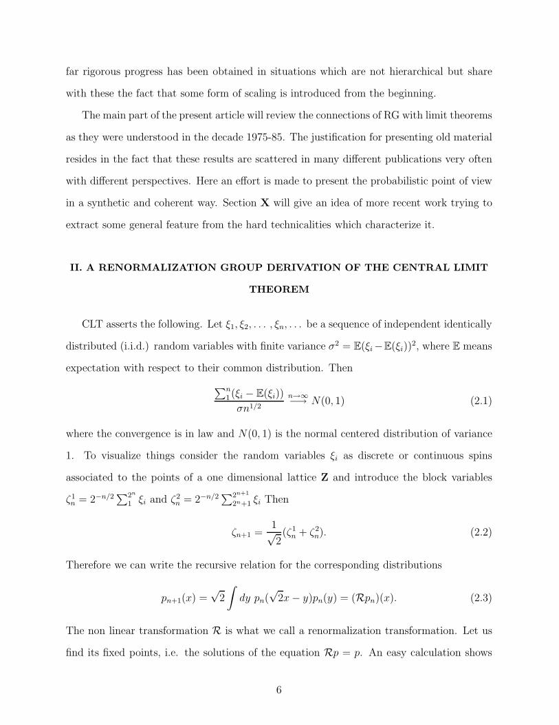
II. A RENORMALIZATION GROUP DERIVATION OF THE CENTRAL LIMIT
THEOREM
CLT asserts the following. Let ξ1, ξ2, . . . , ξn, . . . be a sequence of independent identically
distributed (i.i.d.) random variables with finite variance σ2 = E(ξi−E(ξi))2, where E means
expectation with respect to their common distribution. Then
∑n1 (ξi − E(ξi))
σn1/2
n→∞−→ N(0, 1) (2.1)
where the convergence is in law and N(0, 1) is the normal centered distribution of variance
1. To visualize things consider the random variables ξi as discrete or continuous spins
associated to the points of a one dimensional lattice Z and introduce the block variables
ζ1n = 2−n/2
∑2n
1 ξi and ζ2n = 2−n/2
∑2n+1
2n+1 ξi Then
ζn+1 =1√2(ζ1
n + ζ2n). (2.2)
Therefore we can write the recursive relation for the corresponding distributions
pn+1(x) =√
2
∫
dy pn(√
2x − y)pn(y) = (Rpn)(x). (2.3)
The non linear transformation R is what we call a renormalization transformation. Let us
find its fixed points, i.e. the solutions of the equation Rp = p. An easy calculation shows
6
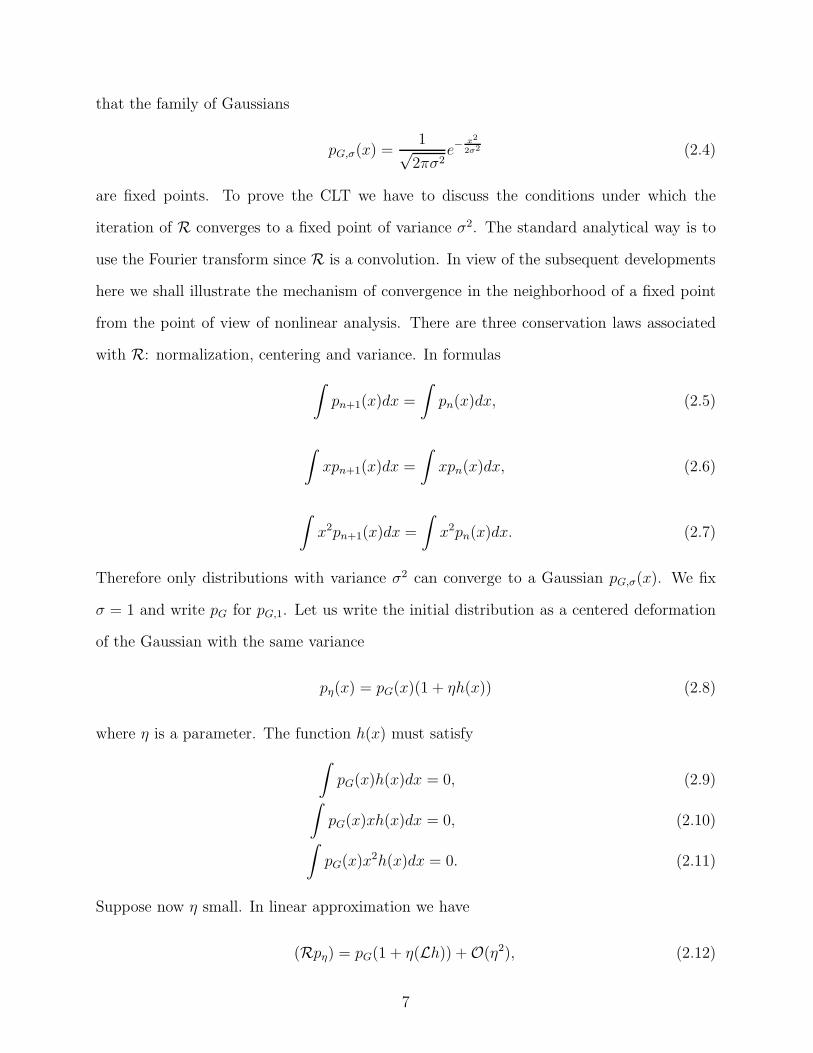
that the family of Gaussians
pG,σ(x) =1√
2πσ2e−
x2
2σ2 (2.4)
are fixed points. To prove the CLT we have to discuss the conditions under which the
iteration of R converges to a fixed point of variance σ2. The standard analytical way is to
use the Fourier transform since R is a convolution. In view of the subsequent developments
here we shall illustrate the mechanism of convergence in the neighborhood of a fixed point
from the point of view of nonlinear analysis. There are three conservation laws associated
with R: normalization, centering and variance. In formulas
∫
pn+1(x)dx =
∫
pn(x)dx, (2.5)
∫
xpn+1(x)dx =
∫
xpn(x)dx, (2.6)
∫
x2pn+1(x)dx =
∫
x2pn(x)dx. (2.7)
Therefore only distributions with variance σ2 can converge to a Gaussian pG,σ(x). We fix
σ = 1 and write pG for pG,1. Let us write the initial distribution as a centered deformation
of the Gaussian with the same variance
pη(x) = pG(x)(1 + ηh(x)) (2.8)
where η is a parameter. The function h(x) must satisfy
∫
pG(x)h(x)dx = 0, (2.9)∫
pG(x)xh(x)dx = 0, (2.10)∫
pG(x)x2h(x)dx = 0. (2.11)
Suppose now η small. In linear approximation we have
(Rpη) = pG(1 + η(Lh)) + O(η2), (2.12)
7

where L is the linear operator
(Lh)(x) = 2π−1/2
∫
dye−y2
h(y + x2−1/2). (2.13)
The eigenvalues of L are
λk = 21−k/2 (2.14)
and the eigenfunctions the Hermite polynomials. The three conditions above on h(x) can
be read as the vanishing of its projections on the first three Hermite polynomials.
The mechanism of convergence of the deformed distribution to the normal law is now
clear in linear approximation: if we develop h in Hermite polynomials only terms with
k > 2 will appear so that upon iteration of the RG transformation they will contract to zero
exponentially as the corresponding eigenvalues are < 1.
To complete the proof one must show that the non linear terms do not alter the conclu-
sion. This is less elementary and will not be pursued here.
A terminological remark. The Gaussian is an example of what is called in probability
theory a stable distribution. These are distributions which are fixed points of convolution
equations and, with the exception of the Gaussian, have infinite variance.
III. HIERARCHICAL MODELS
Suppose now that the ξi are not independent. A case which has played a very important
role in the development of the RG theory of critical phenomena is that of hierarchical models.
To keep the notation close to that of the previous section we write the recursion relation
connecting the distribution at level n to that at level n + 1
pn+1(x) = (Rpn)(x) = gn(x2)(Rpn)(x), (3.1)
where gn(x2) is a sequence of positive increasing functions and R has the same meaning as
in the previous section. It is clear that such a dependence tends to favor large values of the
block variable x and therefore values of the ξi’s of the same sign. We call this a ferromagnetic
8
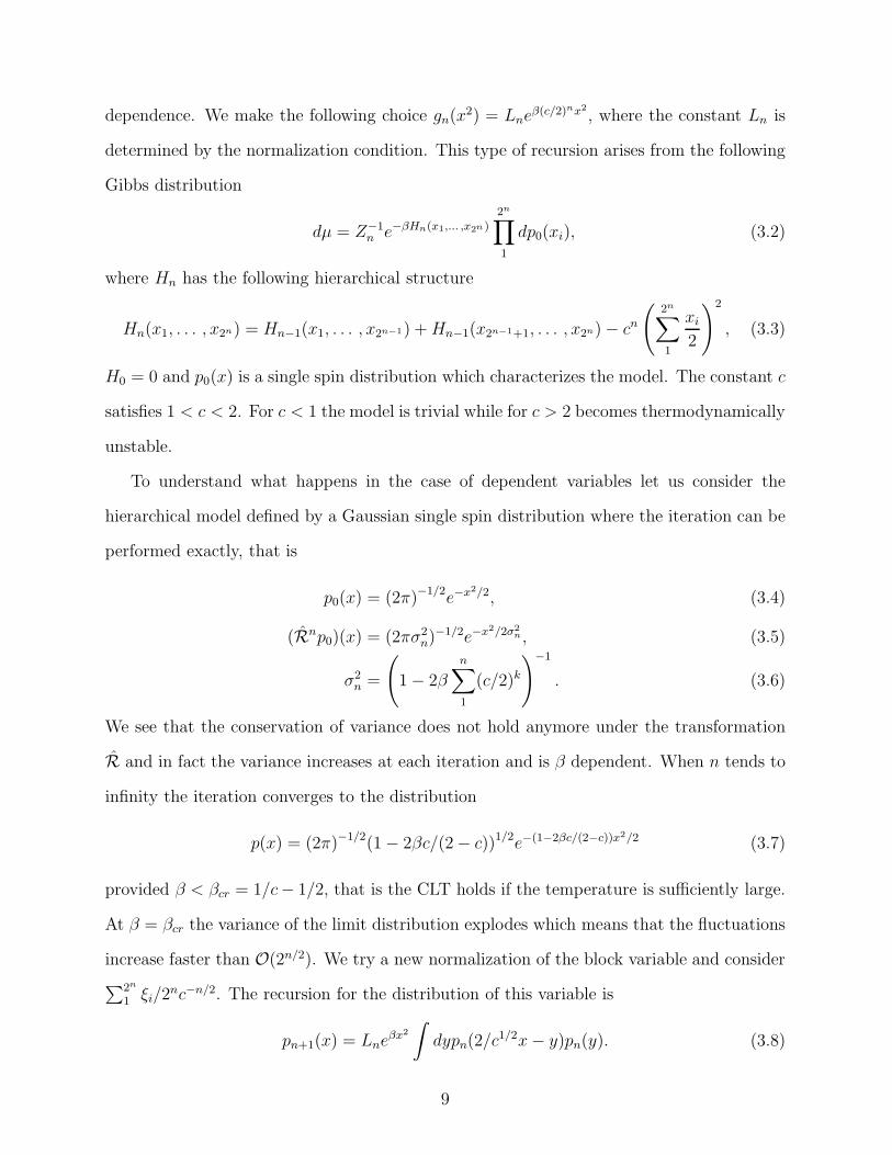
dependence. We make the following choice gn(x2) = Lneβ(c/2)nx2
, where the constant Ln is
determined by the normalization condition. This type of recursion arises from the following
Gibbs distribution
dµ = Z−1n e−βHn(x1,... ,x2n )
2n∏
1
dp0(xi), (3.2)
where Hn has the following hierarchical structure
Hn(x1, . . . , x2n) = Hn−1(x1, . . . , x2n−1) + Hn−1(x2n−1+1, . . . , x2n) − cn
(
2n∑
1
xi
2
)2
, (3.3)
H0 = 0 and p0(x) is a single spin distribution which characterizes the model. The constant c
satisfies 1 < c < 2. For c < 1 the model is trivial while for c > 2 becomes thermodynamically
unstable.
To understand what happens in the case of dependent variables let us consider the
hierarchical model defined by a Gaussian single spin distribution where the iteration can be
performed exactly, that is
p0(x) = (2π)−1/2e−x2/2, (3.4)
(Rnp0)(x) = (2πσ2n)−1/2e−x2/2σ2
n , (3.5)
σ2n =
(
1 − 2β
n∑
1
(c/2)k
)−1
. (3.6)
We see that the conservation of variance does not hold anymore under the transformation
R and in fact the variance increases at each iteration and is β dependent. When n tends to
infinity the iteration converges to the distribution
p(x) = (2π)−1/2(1 − 2βc/(2 − c))1/2e−(1−2βc/(2−c))x2/2 (3.7)
provided β < βcr = 1/c− 1/2, that is the CLT holds if the temperature is sufficiently large.
At β = βcr the variance of the limit distribution explodes which means that the fluctuations
increase faster than O(2n/2). We try a new normalization of the block variable and consider∑2n
1 ξi/2nc−n/2. The recursion for the distribution of this variable is
pn+1(x) = Lneβx2
∫
dypn(2/c1/2x − y)pn(y). (3.8)
9
We now follow the same pattern as in the previous section: calculate the fixed points and see
whether they admit a stable manifold or, in probabilistic language, a domain of attraction.
The fixed points are the solutions of the equation
p(x) = Leβx2
∫
dyp(2/c1/2x − y)p(y) (3.9)
with L determined by normalization. A Gaussian solution is easily found
pG(x) = (a0/π)1/2e−a0x2
(3.10)
with a0 = cβ/(2−c). We shall again discuss stability in linear approximation by considering
a centered deformation of (3.10) pη(x) = pG(x)(1 + ηh(x)). For small η
(Rpη) = pG(1 + η(Lh)) + O(η2). (3.11)
where L is the linear operator
(Lh)(x) =
∫
dye−2a0y2
(h((x + y)/c1/2) + h((x − y)/c1/2)) (3.12)
The corresponding eigenvalues for even eigenfunctions are λ2k = 2/ck, with k = 0, 1, 2, 3, . . . ,
and the eigenfunctions are rescaled Hermite polynomials of even degree.
Here h(x) must be considered as the effect of many iterations starting from some initial
distribution which characterizes the model and is therefore dependent on β. We now see
that for 2 > c > 21/2 the eigenvalues λ0 and λ1 are > 1. The projection of h over the
constants vanishes due to the normalization condition so that for the iteration to converge
we have to impose the vanishing of the projection of h on the second Hermite polynomial.
In view of the previous remark this will select a special value βcr, the critical temperature
for the model considered. In conclusion, for 2 > c > 21/2 and β = βcr the fixed point (3.10)
has a non empty domain of attraction.
When c < 21/2 the Gaussian fixed point becomes unstable and we must investigate about
the existence of other fixed points. Bifurcation theory tells us that most likely there is an
exchange of stability between two fixed points and we should look for the new one in the
10
direction which has just become unstable. For c < 21/2 we have λ4 > 1 so the instability is
in the direction H4, the Hermite polynomial of fourth order. Define ǫ = 21/2 − c and look,
for ǫ small, for a solution of (3.9) of the form
pNG(x) = pG(x)(1 − ǫaH4(γx)) + O(ǫ2) ≈ e−r∗(ǫ)x2/2−u∗(ǫ)x4/4, (3.13)
where r∗ and u∗ are the fixed point couplings. The analysis of this case is considerably more
complicated and gives the following results: the linearization of the RG transformation
around (3.13) has only one unstable direction so that by requiring the vanishing of an
appropriate projection along this direction we obtain a non empty domain of attraction for
some βcr [20], [21].
IV. EIGENVALUES OF THE LINEARIZED RG AND CRITICAL INDICES
We illustrate the interpretation of the eigenvalues of the linearized RG at a fixed point
in the context of hierarchical models, which is especially simple. Notations are as in the
previous section. Consider for definiteness the region 21/3 < c < 21/2 so that the Gaussian
fixed point is unstable, but in its neighborhood there exists a non trivial non Gaussian
fixed point of the form (3.13) with a non empty domain of attraction. Suppose now that
we start the iteration of the RG from some initial distribution which is close to it but not
in its domain of attraction. For example we may consider a distribution p(x, β) of the
form (3.13) with parameters r, u slightly different from r∗, u∗ which are the values taken
at the critical temperature βcr. Application of the RG transformation will eventually drive
this distribution away from the fixed point due to the presence of an unstable direction.
However we can ”renormalize” our parameters r, u by compensating the instability at each
iteration and find a sequence of parameters rn, un such that when n tends to infinity we have
a sequence of distributions pn(x, βn) approaching a definite limit. Since we have assumed
that the parameters rn, un are close to the fixed point values, the renormalized parameters
can be simply expressed in terms of rescalings determined by the eigenvalues of a linear
11
operator analogous to L introduced in the previous section in connection with the Gaussian
fixed point. This can be seen as follows. Let us write our initial distribution as a deformation
of (3.13)
p(x, β) = pNG(x, βcr)(1 + ηh(x, β)). (4.1)
If we develop h in terms of eigenfunctions of the linearized RG at (3.13), the iteration of the
RG transformation will multiply the projections of h along these eigenfunctions by powers of
the corresponding eigenvalues. The explosion in the unstable direction can then be controlled
by rescaling at each step the projection in this direction with a factor proportional to the
inverse eigenvalue.
Let us define the susceptibility of a block of 2n spins
χn(β) =1
2nE
(
2n∑
1
ξi
)2
(4.2)
This quantity can be easily expressed in terms of the distribution pn(x, β) of the block with
the critical normalization 2nc−n/2
χn(β) = (2/c)n
∫
dxx2pn(x, β). (4.3)
As n → ∞, χn diverges if β = βcr.
To calculate the susceptibility critical index as β approaches the critical value we assume
that the two limits n → ∞ and β → βcr can be interchanged so that they can be calculated
over subsequences. We want to compute
νχ = limn→∞
log χn(βn)
log |βn − βcr|= lim
n→∞
−n log(c/2) + log∫
dy y2pn(y, βn)
log |βn − βcr|. (4.4)
If we now choose |βn − βcr| ≈ λ−n, where λ is the eigenvalue corresponding to the unstable
direction of the RG linearized at the fixed point, the integral appearing in this formula will
be almost constant and we obtain
νχ =log(c/2)
log λ. (4.5)
12
Similar calculations can be done for other thermodynamical quantities like the free energy
or the magnetization.
We can summarize the situation as follows: given a model defined by an initial distribu-
tion p0, for β < βcr we expect the CLT to hold. For β = βcr by properly normalizing the
block variables we have new limit theorems where the limit law has a domain of attraction
which is a non trivial submanifold in the space of probability distributions called the critical
manifold. If we start from a distribution which is not in the domain of attraction of a given
fixed point, but not too far from it, it can still be driven to a regular limit by rescaling at
each step its coefficients in a way dictated by the fixed point. This defines the so called
scaling limits of the theory associated to a given fixed point.
For further reading see [21], [22], [23].
V. SELF SIMILAR RANDOM FIELDS
The notion of self similar random field was introduced informally in [16] and rigorously
in [17] and independently in [18]. It was then developed more systematically in [24] and
[25]. The idea was to construct a proper mathematical setting for the notion of RG a la
Kadanoff-Wilson. This led to a generalization of limit theorems for random fields to the
situation in which the variables are strongly correlated.
Let Zd be a lattice in d-dimensional space and j a generic point of Zd, j = (j1, j2, ..., jd)
with integer coordinates ji. We associate to each site a centered random variable ξj and
define a new random field
ξnj = (Rα,nξ)j = n−dα/2
∑
s∈V nj
ξs, (5.1)
where
V nj = {s : jkn − n/2 < sk ≤ jkn + n/2} (5.2)
and 1 ≤ α < 2. The transformation (5.1) induces a transformation on probability measures
13
according to
(R∗α,nµ)(A) = µ′(A) = µ(R−1
α,nA), (5.3)
where A is a measurable set and R∗α,n has the semigroup property
R∗α,n1
R∗α,n2
= R∗α,n1+n2
. (5.4)
A measure µ will be called self similar if
R∗α,nµ = µ (5.5)
and the corresponding field will be called a self similar random field. We briefly discuss the
choice of the parameter α. It is natural to take 1 ≤ α < 2. In fact α = 2 corresponds
to the law of large numbers so that the block variable (5.1) will tend for large n to zero
in probability. The case α > 1 means that we are considering random systems which
fluctuate more than a collection of independent variables and α = 1 corresponds to the
CLT. Mathematically the lower bound is not natural but it becomes so when we restrict
ourselves to the consideration of ferromagnetic-like systems.
A general theory of self similar random fields so far does not exist and presumably is very
difficult. However Gaussian fields are completely specified by their correlation function and
self similar Gaussian fields can be constructed explicitly [18], [26]. It is easier if we represent
the correlation function in terms of its Fourier transform
E(ξiξj) =
∫ π
−π
d∏
1
dλkρ(λ1, . . . , λd)ei∑
k λk(i−j)k . (5.6)
The prescription to construct ρ in such a way that the corresponding Gaussian field satisfies
(5.5) is as follows. Take a positive homogeneous function f(λ1, ..., λd) with homogeneity
exponent d(1 + α), that is
f(cλ1, ..., cλd) = cd(1+α)f(λ1, ..., λd) (5.7)
. Next we construct a periodic function g(λ1, ..., λd) by taking an average over the lattice
Zd
g(λ1, ..., λd) =∑
ik
1
f(λ1 + i1, . . . , λd + id). (5.8)
14
If we take now
ρ(λ1, . . . , λd) =∏
i
|1 − eiλi|2g(λ1, . . . , λd), (5.9)
it is not difficult to see that the corresponding Gaussian measure satisfies (5.5). The peri-
odicity of ρ insures translational invariance.
For d = 1 there is only one, apart from a multiplicative constant, homogeneous function
and one can show that the above construction exhausts all possible Gaussian self similar
distributions. For d > 1 it is not known whether a similar conclusion holds.
From this point on one can follow in the discussion the same pattern as for hierarchical
models and investigate the stability of the Gaussian fixed points PG of (5.5). Consider a
deformation PG(1 + h) and the action of R∗α,n on this distribution. It is easily seen that
R∗α,nPGh = E(h|{ξn
j })R∗α,nPG = E(h|{ξn
j })PG({ξnj }). (5.10)
The conditional expectation on the right hand side of (5.10) will be called the linearization
of the RG at the fixed point PG. To proceed further in the study of the stability we have to
find its eigenvectors and eigenvalues. These have been calculated by Sinai. The eigenvectors
are appropriate infinite dimensional generalizations of Hermite polynomials Hk which are
described in full detail in [26]. They satisfy the eigenvalue equation
E(Hk|{ξnj }) = n[k(α/2−1)+1]dHk({ξn
j }). (5.11)
We see immediately that H2 is always unstable while H4 becomes unstable when α crosses
from below the value 3/2. By introducing the parameter ǫ = α − 3/2, in principle one can
construct, as in the hierarchical case, a non Gaussian fixed point. The formal construction
is explained in Sinai’s book [26] where one can find also an exhaustive discussion of the
questions, mostly unsolved, arising in this connection. A different construction of a non
Gaussian fixed point, for d = 4 has been made recently by Brydges, Dimock and Hurd. This
will be briefly discussed in section X.
15
VI. SOME PROPERTIES OF SELF SIMILAR RANDOM FIELDS
We have already characterized the critical point as a situation of strongly dependent
random variables, in which the CLT fails. We want to give here a characterization which
refers to the random field globally. Consider in the product space of the variables ξi the
cylinder sets, that is the sets of the form
{ξi1 ∈ A1, . . . , ξin ∈ An}, (6.1)
with i1, . . . , in ∈ Λ, Λ being an arbitrary finite region in Zd and the Ai measurable sets in
the space of the variables ξi. We denote with ΣΛ the σ-algebra generated by such sets. We
say that the variables ξi are weakly dependent or that they are a strong mixing random field
if the following holds. Given two finite regions Λ1 and Λ2 separated by a distance
d(Λ1, Λ2) = mini∈Λ1,j∈Λ2
|i − j|, (6.2)
where |i − j| is for example the Euclidean distance, define
τ(Λ1, Λ2) = supA∈ΣΛ1
,B∈ΣΛ2
|µ(A ∩ B) − µ(A)µ(B)|. (6.3)
Then τ(Λ1, Λ2) → 0 when d(Λ1, Λ2) → ∞.
Intuitively the strong mixing idea is that one cannot compensate for the weakening of
the dependence of the variables due to an increase of their space distance, by increasing the
size of the sets.
This situation is typical when one has exponential decay of correlations. This has been
proved for a wide class of random fields including ferromagnetic non critical spin systems
[27].
The situation is entirely different at the critical point where one expects the correlations
to decay as an inverse power of the distance. In this connection the following result has
been proved in [28]: a ferromagnetic translational invariant system with pair interactions
with correlation function
C(i) = E(ξ0ξi) − E(ξ0)E(ξi) (6.4)
16
such that
limL→∞
∑
L(sk−1)≤ik<L(sk+1) C(i)∑
0≤ik<L C(i)6= 0 (6.5)
for arbitrary sk, does not satisfy the strong mixing condition.
This theorem implies in particular that a critical 2-dimensional Ising model violates
strong mixing. Therefore violation of strong mixing seems to provide a reasonable char-
acterization of the type of strong dependence encountered in critical phenomena. On the
other end, under very general conditions, if strong mixing holds the one-block distribution
satisfies the CLT [29].
An interesting question is whether we can describe the structure of the limit one-block
distributions that can appear at the critical point beside the Gaussian. It was shown in
[28], building on previous results by Newman, that for ferromagnetic systems the Fourier
transform (characteristic function in probabilistic language) of the limit distribution must
be of the form
E(eitξ) = e−bt2∏
j
(1 − t2/α2j ) (6.6)
with∑
j 1/α2j < ∞. In the probabilistic literature these distributions are called the D-class
[36]. The Gaussian is the only infinitely divisible distribution belonging to this class.
VII. MULTIPLICATIVE STRUCTURE
In this section we show that there is a natural multiplicative structure associated with
transformations on probability distributions like those induced by the RG. This multiplica-
tive structure is related to the properties of conditional expectations. We use the notations
of section V. Suppose we wish to evaluate the conditional expectation
E(h|{ξnj }), (7.1)
where the collection of block variables ξnj indexed by j is given a fixed value. Here h is a
function of the individual spins ξi. It is an elementary property of conditional expectations
17
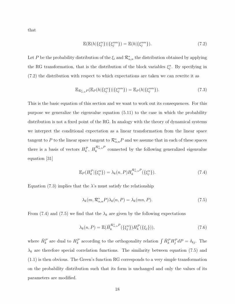
that
E(E(h|{ξnj })|{ξnm
j }) = E(h|{ξnmj }). (7.2)
Let P be the probability distribution of the ξi and R∗α,n the distribution obtained by applying
the RG transformation, that is the distribution of the block variables ξnj . By specifying in
(7.2) the distribution with respect to which expectations are taken we can rewrite it as
ER∗α,nP (EP (h|{ξn
j })|{ξnmj }) = EP (h|{ξnm
j }). (7.3)
This is the basic equation of this section and we want to work out its consequences. For this
purpose we generalize the eigenvalue equation (5.11) to the case in which the probability
distribution is not a fixed point of the RG. In analogy with the theory of dynamical systems
we interpret the conditional expectation as a linear transformation from the linear space
tangent to P to the linear space tangent to R∗α,nP and we assume that in each of these spaces
there is a basis of vectors HPk , H
R∗α,nP
k connected by the following generalized eigenvalue
equation [31]
EP (HPk |{ξn
j }) = λk(n, P )HR∗
α,nP
k ({ξnj }). (7.4)
Equation (7.3) implies that the λ’s must satisfy the relationship
λk(m,R∗α,nP )λk(n, P ) = λk(mn, P ). (7.5)
From (7.4) and (7.5) we find that the λk are given by the following expectations
λk(n, P ) = E(HR∗
α,nP
k ({ξnj })HP
k ({ξj})), (7.6)
where HPk are dual to HP
k according to the orthogonality relation∫
HPk HP
j dP = δkj. The
λk are therefore special correlation functions. The similarity between equation (7.5) and
(1.1) is then obvious. The Green’s function RG corresponds to a very simple transformation
on the probability distribution such that its form is unchanged and only the values of its
parameters are modified.
18
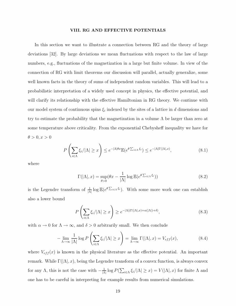
VIII. RG AND EFFECTIVE POTENTIALS
In this section we want to illustrate a connection between RG and the theory of large
deviations [32]. By large deviations we mean fluctuations with respect to the law of large
numbers, e.g., fluctuations of the magnetization in a large but finite volume. In view of the
connection of RG with limit theorems our discussion will parallel, actually generalize, some
well known facts in the theory of sums of independent random variables. This will lead to a
probabilistic interpretation of a widely used concept in physics, the effective potential, and
will clarify its relationship with the effective Hamiltonian in RG theory. We continue with
our model system of continuous spins ξi indexed by the sites of a lattice in d dimensions and
try to estimate the probability that the magnetization in a volume Λ be larger than zero at
some temperature above criticality. From the exponential Chebysheff inequality we have for
θ > 0, x > 0
P
(
∑
i∈Λ
ξi/|Λ| ≥ x
)
≤ e−|Λ|θxE(eθ
∑
i∈Λ ξi) ≤ e−|Λ|Γ(|Λ|,x), (8.1)
where
Γ(|Λ|, x) = supθ>0
(θx − 1
|Λ| log E(eθ∑
i∈Λ ξi)) (8.2)
is the Legendre transform of 1|Λ|
log E(eθ∑
i∈Λ ξi). With some more work one can establish
also a lower bound
P
(
∑
i∈Λ
ξi/|Λ| ≥ x
)
≥ e−|Λ|(Γ(|Λ|,x)+α(|Λ|)+δ), (8.3)
with α → 0 for Λ → ∞, and δ > 0 arbitrarily small. We then conclude
− limΛ→∞
1
|Λ| log P
(
∑
i∈Λ
ξi/|Λ| ≥ x
)
= limΛ→∞
Γ(|Λ|, x) = Veff(x), (8.4)
where Veff (x) is known in the physical literature as the effective potential. An important
remark. While Γ(|Λ|, x), being the Legendre transform of a convex function, is always convex
for any Λ, this is not the case with − 1|Λ|
log P (∑
i∈Λ ξi/|Λ| ≥ x) = V (|Λ|, x) for finite Λ and
one has to be careful in interpreting for example results from numerical simulations.
19
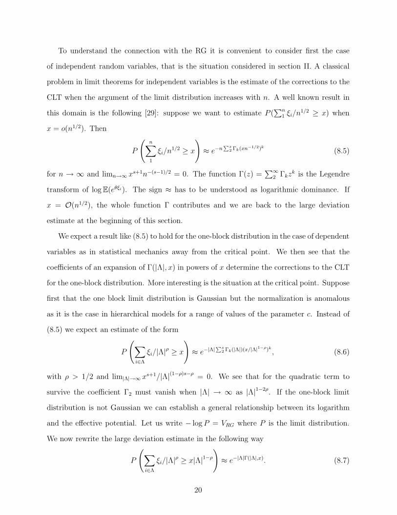
To understand the connection with the RG it is convenient to consider first the case
of independent random variables, that is the situation considered in section II. A classical
problem in limit theorems for independent variables is the estimate of the corrections to the
CLT when the argument of the limit distribution increases with n. A well known result in
this domain is the following [29]: suppose we want to estimate P (∑n
1 ξi/n1/2 ≥ x) when
x = o(n1/2). Then
P
(
n∑
1
ξi/n1/2 ≥ x
)
≈ e−n∑s
2 Γk(xn−1/2)k
(8.5)
for n → ∞ and limn→∞ xs+1n−(s−1)/2 = 0. The function Γ(z) =∑∞
2 Γkzk is the Legendre
transform of log E(eθξi). The sign ≈ has to be understood as logarithmic dominance. If
x = O(n1/2), the whole function Γ contributes and we are back to the large deviation
estimate at the beginning of this section.
We expect a result like (8.5) to hold for the one-block distribution in the case of dependent
variables as in statistical mechanics away from the critical point. We then see that the
coefficients of an expansion of Γ(|Λ|, x) in powers of x determine the corrections to the CLT
for the one-block distribution. More interesting is the situation at the critical point. Suppose
first that the one block limit distribution is Gaussian but the normalization is anomalous
as it is the case in hierarchical models for a range of values of the parameter c. Instead of
(8.5) we expect an estimate of the form
P
(
∑
i∈Λ
ξi/|Λ|ρ ≥ x
)
≈ e−|Λ|∑s
2 Γk(|Λ|)(x/|Λ|1−ρ)k
, (8.6)
with ρ > 1/2 and lim|Λ|→∞ xs+1/|Λ|(1−ρ)s−ρ = 0. We see that for the quadratic term to
survive the coefficient Γ2 must vanish when |Λ| → ∞ as |Λ|1−2ρ. If the one-block limit
distribution is not Gaussian we can establish a general relationship between its logarithm
and the effective potential. Let us write − log P = VRG where P is the limit distribution.
We now rewrite the large deviation estimate in the following way
P
(
∑
i∈Λ
ξi/|Λ|ρ ≥ x|Λ|1−ρ
)
≈ e−|Λ|Γ(|Λ|,x). (8.7)
20
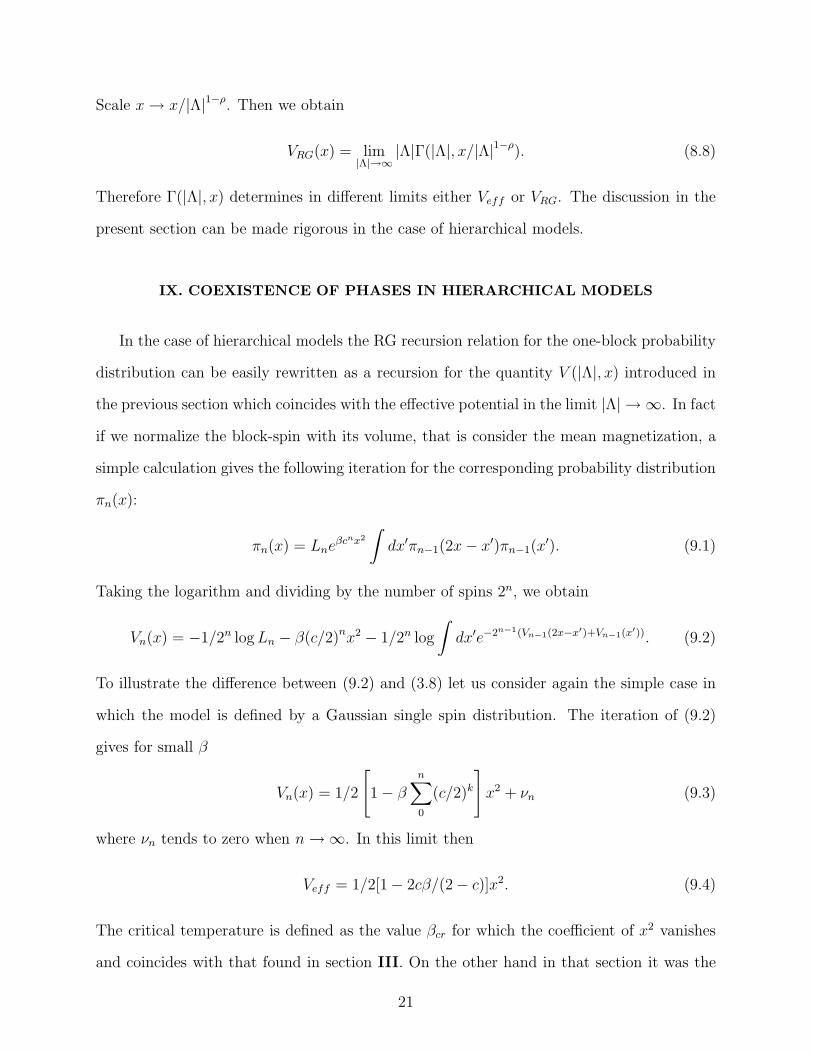
Scale x → x/|Λ|1−ρ. Then we obtain
VRG(x) = lim|Λ|→∞
|Λ|Γ(|Λ|, x/|Λ|1−ρ). (8.8)
Therefore Γ(|Λ|, x) determines in different limits either Veff or VRG. The discussion in the
present section can be made rigorous in the case of hierarchical models.
IX. COEXISTENCE OF PHASES IN HIERARCHICAL MODELS
In the case of hierarchical models the RG recursion relation for the one-block probability
distribution can be easily rewritten as a recursion for the quantity V (|Λ|, x) introduced in
the previous section which coincides with the effective potential in the limit |Λ| → ∞. In fact
if we normalize the block-spin with its volume, that is consider the mean magnetization, a
simple calculation gives the following iteration for the corresponding probability distribution
πn(x):
πn(x) = Lneβcnx2
∫
dx′πn−1(2x − x′)πn−1(x′). (9.1)
Taking the logarithm and dividing by the number of spins 2n, we obtain
Vn(x) = −1/2n log Ln − β(c/2)nx2 − 1/2n log
∫
dx′e−2n−1(Vn−1(2x−x′)+Vn−1(x′)). (9.2)
To illustrate the difference between (9.2) and (3.8) let us consider again the simple case in
which the model is defined by a Gaussian single spin distribution. The iteration of (9.2)
gives for small β
Vn(x) = 1/2
[
1 − βn∑
0
(c/2)k
]
x2 + νn (9.3)
where νn tends to zero when n → ∞. In this limit then
Veff = 1/2[1 − 2cβ/(2 − c)]x2. (9.4)
The critical temperature is defined as the value βcr for which the coefficient of x2 vanishes
and coincides with that found in section III. On the other hand in that section it was the
21
only temperature for which the recursion (3.8) converges to the Gaussian fixed point, i.e.
the only temperature for which the following difference between two diverging expressions
converges
2β
n∑
0
(2/c)k − (2/c)n+1. (9.5)
We want to apply now (9.2) to the study of the magnetization in the phase coexistence
region for a general hierarchical model [33], [34]. The problem we want to discuss is the
following. In the hierarchical case at level n we have blocks, containing each 2n−1 spins,
interacting in pairs through the Hamiltonian
cn(ζ1n−1 + ζ2
n−1)2/4 = cn(ζn)2 (9.6)
where ζ1n−1, ζ
2n−1, ζn are mean magnetizations. Suppose now that ζn is assigned the value
αM , 0 < α < 1, M being the spontaneous magnetization corresponding to the temperature
β. We want to calculate the conditional distribution of ζn−1 given ζn, for large n. The
remarkable result is that one of the quantities ζ1n−1 or ζ2
n−1 with probability close to 1 is
equal to the full magnetization M .
To compute the desired distribution we have to estimate πn(x) or, what is the same,
Vn(x) for large n. From (9.2) we expect asymptotically
Vn(x) = Veff (x) + (c/2)nY (x) + . . . (9.7)
Since in the phase coexistence region Veff(x) is flat, i.e. constant, the whole x dependence
is given by Y (x). In order to compute this function we perform a subtraction and consider
Vn(x)−Vn(x0) choosing x0 in the flat region of Veff(x). From (9.2) it is easily seen that the
quantity
∆n(x) = (2/c)n(Vn(x) − Vn(x0)) (9.8)
satisfies a recursion of the form
∆n(x) = −c−n log An − βx2 − c−n log
∫
dx′e−cn−1(∆n−1(x+x′)+∆n−1(x−x′)), (9.9)
22
where An is determined by the condition ∆n(x0) = 0. Let us choose x0 = M . By symmetry
∆n(±M) = 0. For 0 ≤ x ≤ M and large n the main contribution to the integral on the
right hand side of (9.9) comes from the region x± x′ ≈ M , while for −M ≤ x ≤ 0 from the
region x ± x′ ≈ −M . We can write therefore the approximate recursion equations
∆n(x) = β(M2 − x2) + c−1∆n−1(2x ∓ M), (9.10)
where the ∓ in the second term on the right corresponds to 0 ≤ x ≤ M or −M ≤ x ≤ 0. This
type of equations has been rigorously studied by Bleher [33] and the asymptotic solutions
show a complicated fractal structure.
The conditional probability of interest to us is
P (|ζn−1 − M | < ǫM |ζn = αM) =
∫
|x′−M |<ǫMdx′e−cn−1(∆n−1(x′)+∆n−1(2αM−x′))
∫∞
∞dx′e−cn−1(∆n−1(x′)+∆n−1(2αM−x′))
(9.11)
Since the main contribution to the integral in the denominator comes from the same region
appearing in the numerator, our conditional probability is for sufficiently large n as close as
we want to 1.
X. WEAK PERTURBATIONS OF GAUSSIAN MEASURES:
A NON GAUSSIAN FIXED POINT
Starting at the end of the seventies the RG has become a very important and effective
tool for proving rigorous results in statistical mechanics and Euclidean quantum field theory.
An impressive amount of work has been done and it is not possible to give even a schematic
account of it [35]. Many different versions of the RG idea have been used, each author or
group of authors following his own linguistic propensities. Probability theory is always in
the background and we want to try to recover some conceptual feature common to all of
them. As in the previous part of this review limit theorems will be a relevant reference.
However the limit theorems to be considered are of a different kind, they are those which in
probability are called non classical and are related to the following problem.
23
Given a probability distribution P and an integer n, can one consider it as resulting
from the composition (convolution) of n distributions Pk, k = 1, 2, . . . , n? In other words
can one consider the random variable described by P as the sum of n independent random
variables? In formulas
P = P1 ⋆ P2 ⋆ . . . ⋆ Pn, (10.1)
where ⋆ means convolution. It is clear, for example, that a Gaussian distribution of variance
σ2 can be thought as the composition of any number n of Gaussians with variances σ2i
provided∑n
1 σ2i = σ2. The problem arises naturally of investigating under what conditions
convolutions like the right hand side of (10.1) converge to a regular distribution as n → ∞.
The right hand side of (10.1) can be considered as a recurrence relation
Pn+1 = Pn ⋆ Pn, (10.2)
where Pn = P1 ⋆P2 ⋆ . . . ⋆Pn−1. Comparing (2.3) with (10.1) we see that while in the case of
limit theorems for independent identically distributed random variables we have a natural
fixed point problem, this is not in general the case for non identically distributed variables.
As we shall see below, the RG approach to Euclidean field theory and the statistical mechan-
ics of the critical point has led to formulations which have analogies with these problems.
In fact, infinite dimensional equations structurally similar to (10.2) are constructed which
can be transformed into equations admitting fixed points after a rescaling.
In the following exposition we shall follow the recent article by Brydges, Dimock and
Hurd [37]. The goal of these authors is the construction of a quantum field theory in R4 with
non trivial scaling behaviour at long distances, that is in the infrared region, determined by
a non Gaussian fixed point of an appropriate RG transformation. The starting point is a φ4
theory in finite volume regularized at small distances to eliminate ultraviolet singularities.
This model is believed to have a non Gaussian fixed point in 4−ǫ dimensions and to simulate
such a situation in 4 dimensions the authors introduce a special covariance for the Gaussian
part of the measure. The first step consists in the construction of a covariance v(x − y)
24

which behaves at large distances like (−∆)−1−ǫ/2. This means that it scales like |x|−2+ǫ for
large |x|. Their choice is
v(x − y) =
∫ ∞
1
dααǫ/2−2e−|x−y|2/4α. (10.3)
Such a covariance can be decomposed in the following way
v(x − y) =
∞∑
j=0
L−(2−ǫ)jC(L−j(x − y)), (10.4)
where L > 1 is a scaling factor and
C(x) =
∫ L2
1
dααǫ/2−2e−|x|2/4α. (10.5)
Each term in the expansion can be interpreted as the covariance of a rescaled field
φL−j(x) = L−(2−ǫ)j/2φ(L−jx) (10.6)
which has reduced fluctuations and varies over larger distances. The aim is to study the
measure
dµΛ = Z−1e−VΛ(φ)dµv (10.7)
where
VΛ(φ) = λ
∫
Λ
: φ4 :v + ζ
∫
Λ
: (∂φ)2 :v + µ
∫
Λ
: φ2 :v (10.8)
when Λ tends to R4. The double dots indicate the Wick polynomials with respect to the
covariance v.
Take for Λ a large cube of side LN so that the measure is well defined. We want to
calculate
(µv ⋆ e−V )(φ) = (µCN⋆ µCN−1
⋆ .... ⋆ µC0⋆ e−V )(φ) (10.9)
having used the above decomposition of the covariance with
Cj(x) = L−(2−ǫ)jC(L−j(x − y)) (10.10)
25
Actually in finite volume we should specify some boundary conditions but we shall ignore
this aspect. Next by defining
Zj(φ) = (µCj−1⋆ . . . ⋆ µC0
⋆ e−V )(φ) (10.11)
we find the recursion relation
Zj+1(φ) = (µCj⋆ Zj)(φ). (10.12)
In this way the calculation is performed by successive integrations over variables which
exhibit decreasing fluctuations. This is not yet our RG equation because as j → ∞, µCj
becomes a singular distribution and we do not obtain a fixed point equation. However by
introducing the rescaled fields φL−j (x) = L−(2−ǫ)j/2φ(L−jx) and the rescaled Z’s
Zj(φ) = Zj(φL−j ) (10.13)
the recursion becomes
Zj+1(φ) = (µC ⋆ Zj)(φL−1) (10.14)
with initial condition Z0 = e−V . We emphasize that the last step is possible due to the
special structure of the measures µCj. It is now meaningful to look for the fixed points of
(10.14). Brydges, Dimock and Hurd have proved that in d = 4 for ǫ small there exists a
non Gaussian fixed point of (10.14) characterized by a value λ(ǫ, L) of the coupling λ and
that for certain values µ(λ), ζ(λ) the iteration of (10.14) with initial condition e−V converges
to this fixed point. Technically the proof is very complicated and its description is beyond
the aims of this review. A very good exposition with some simplifications of the techniques
employed can be found also in [38].
XI. CONCLUDING REMARKS
The question we want to consider is the following: which are the benefits for our un-
derstanding of critical phenomena and more generally of statistical physics deriving from
26
the use of probabilistic language? Feynman thought that it is worth to spend one’s time
formulating a theory in every physical and mathematical way possible. In our case there is
an intuition associated with probabilistic reasoning that is foreign to the usual formalisms
of statistical mechanics based on correlation functions and equations connecting them.
Apart from this general remark we must consider that the rigorous results obtained so far
in RG theory have been strongly influenced by the probabilistic language as this appears the
most natural for the mathematical study of statistical mechanics and Euclidean field theory
when a functional integral approach is used. New technical ideas however are needed to deal
with concrete problems like calculating the critical indices of the 3-dimensional Ising model
or establishing in a conclusive way whether the field theory φ44 is ultraviolet non trivial.
The formal apparatus of RG has been easily extended to the analysis of fermionic sys-
tems when these are described by a Grassmaniann functional integral [39], that is by the
analog of a Gibbs distribution over anticommuting variables. In this case the convergence of
perturbation theory plays a major role on the way to rigorous results. Recently, it has been
possible to give a true probabilistic expression to general Grassmaniann integrals in terms
of discrete jump processes (Poisson processes) [40], [41] so that classical probability may
become a main tool also in the study of fermionic systems especially in view of developing
non perturbative methods. For an early example of connection between anticommutative
calculus and probability see [42].
In a wider perspective one may remark that the theory of Gibbs distributions is becom-
ing instrumental also in various sectors of mathematical statistics, for example in image
reconstruction, and critical situations appear also in this domain. Transfer of ideas from
statistical mechanics to stochastic analysis is currently an ongoing process which shows the
relevance of a language capable of unifying different areas of research. Probability theory
for a long time has not been included among the basic mathematical tools of a physics cur-
riculum but the situation is slowly changing and hopefully this will help cross fertilization
among different disciplines.
27

ACKNOWLEDGMENTS
This paper is an expanded version of a talk given at the meeting RG 2000, Taxco,
Mexico, January 1999. It is a pleasure to thank C. Stephens and D. O’ Connor for their
kind invitation.
28
REFERENCES
[1] A. I. Khinchin Mathematical Foundations of Statistical Mechanics Dover Publications
Inc. N. Y., 1949.
[2] C. Di Castro, G. Jona-Lasinio Phys. Letts. 29A, 322 (1969).
[3] K. G. Wilson, M. E. Fisher Phys. Rev. Letts. 28, 240 (1972).
[4] C. Di Castro Lett. al Nuovo Cim. 5, 69 (1972).
[5] P. K. Mitter Phys.Rev. D7, 2927 (1973).
[6] E. Brezin, J. C. Le Guillou, J. Zinn Justin Phys. Rev. D8, 434 (1973).
[7] K. G. Wilson Phys. Rev. B4, 3174 (1971).
[8] K. G. Wilson 140, B445 (1965).
[9] K. G. Wilson Phys. Rev. D2, 1438 (1970).
[10] L. P. Kadanoff Physics (N. Y.) 2, 263 (1966).
[11] G. Jona-Lasinio in Nobel Symposium 24, 38 (1973).
[12] G. Benettin, C. Di Castro, G. Jona-Lasinio, L. Peliti, A. L. Stella in New Developments
in Quantum Field Theory and Statistical Mechanics, M. Levy and P. K. Mitter eds.,
Plenum Press, New York, London, 1977.
[13] M. E. Fisher Rev. Mod. Phys. 70, 653 (1998).
[14] A. Z. Patashinski, V. L. Pokrovski Fluctuation Theory of Phase Transitions 2nd edition,
Nauka, Moskva 1982 (Russian).
[15] P. M. Bleher, Ya. G. Sinai Comm. Math. Phys 33, 23 (1973).
[16] G. Jona-Lasinio Nuovo Cim. B 26, 9 (1975).
[17] G. Gallavotti, G. Jona-Lasinio Comm. Math. Phys. 41, 301 (1975).
29
[18] Ya. G. Sinai Theor. Prob. Appl. 21, 273 (1976).
[19] G. Jona-Lasinio in New Developments in Quantum Field Theory and Statistical Me-
chanics, M. Levy and P. K. Mitter eds., Plenum Press, New York, London, 1977.
[20] P. M. Bleher, Ya. G. Sinai Comm. Math. Phys 45, 347 (1975)
[21] P. Collet, J. P. Eckmann A Renormalization Group Analysis of the Hierarchical Model
in Statistical Mechanics, Lecture Notes in Phys. 74, Springer-Verlag 1978.
[22] M. Cassandro, G. Gallavotti Nuovo Cim. 25B, 691 (1975).
[23] G. Gallavotti, H. Knops Rivista del Nuovo Cim. 5, 341 (1975).
[24] R. L. Dobrushin in Multicomponent Random Systems, Dekker, N. Y., 1978.
[25] R. L. Dobrushin Ann. of Prob. 7, 1 (1979).
[26] Ya. G. Sinai Theory of Phase Transitions: Rigorous Results, Pergamon Press, London
1982.
[27] G. Hegerfeldt, C. Nappi, Comm. Math. Phys. 53, 1 (1977).
[28] M. Cassandro, G. Jona-Lasinio in Many Degrees of Freedom in Field Theory, L. Streit
ed., Plenum Press 1978.
[29] I. A. Ibragimov, Yu. V. Linnik Independent and Stationary Sequences of Random Vari-
ables, Wolters-Noordhoff, Groningen 1971.
[30] M. Cassandro, G. Jona-Lasinio Adv. Phys. 27, 913 (1978).
[31] V. I. Oseledec Trans. Moscow Math. Soc. 19, 197 (1968).
[32] G. Jona-Lasinio in Scaling and Self-similarity in Physics, J. Frolich ed., Birkhauser 1983.
[33] P. M. Bleher Theor. and Math. Phys. 61, 1107 (1985).
[34] G. Jona-Lasinio Helv. Phys. Acta 59, 234 (1986).
30
[35] A basic reference is G. Gallavotti Rev. Mod. Phys. 57, 471 (1985).
[36] Yu. V. Linnik, I. V. Ostrovski Decomposition of Random Variables and Vectors Transl.
of Math. Monographs, AMS, 1977.
[37] D. Brydges, J. Dimock, T. R. Hurd Comm. Math. Phys. 198, 111 (1998).
[38] P. K. Mitter, B. Scoppola Comm. Math. Phys. 209, 207 (2000).
[39] G. Benfatto, G. Gallavotti Renormalization Group, Physics Notes, Princeton University
Press 1995.
[40] G. F. De Angelis, G. Jona-Lasinio, V. Sidoravicius J. Phys. A 31, 289 (1998).
[41] M. Beccaria, C. Presilla, G. F. De Angelis, G. Jona-Lasinio Europhys. Lett. 48, 243
(1999).
[42] D. Brydges, I. Munoz Maya J. Theor. Prob. 4, 371 (1991).
31


