
Regression Models For Count Data
Statistics 149
Spring 2006
Copyright ©2006 by Mark E. Irwin
Poisson Regression Model
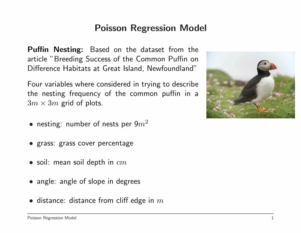
Puffin Nesting: Based on the dataset from thearticle ”Breeding Success of the Common Puffin onDifference Habitats at Great Island, Newfoundland”
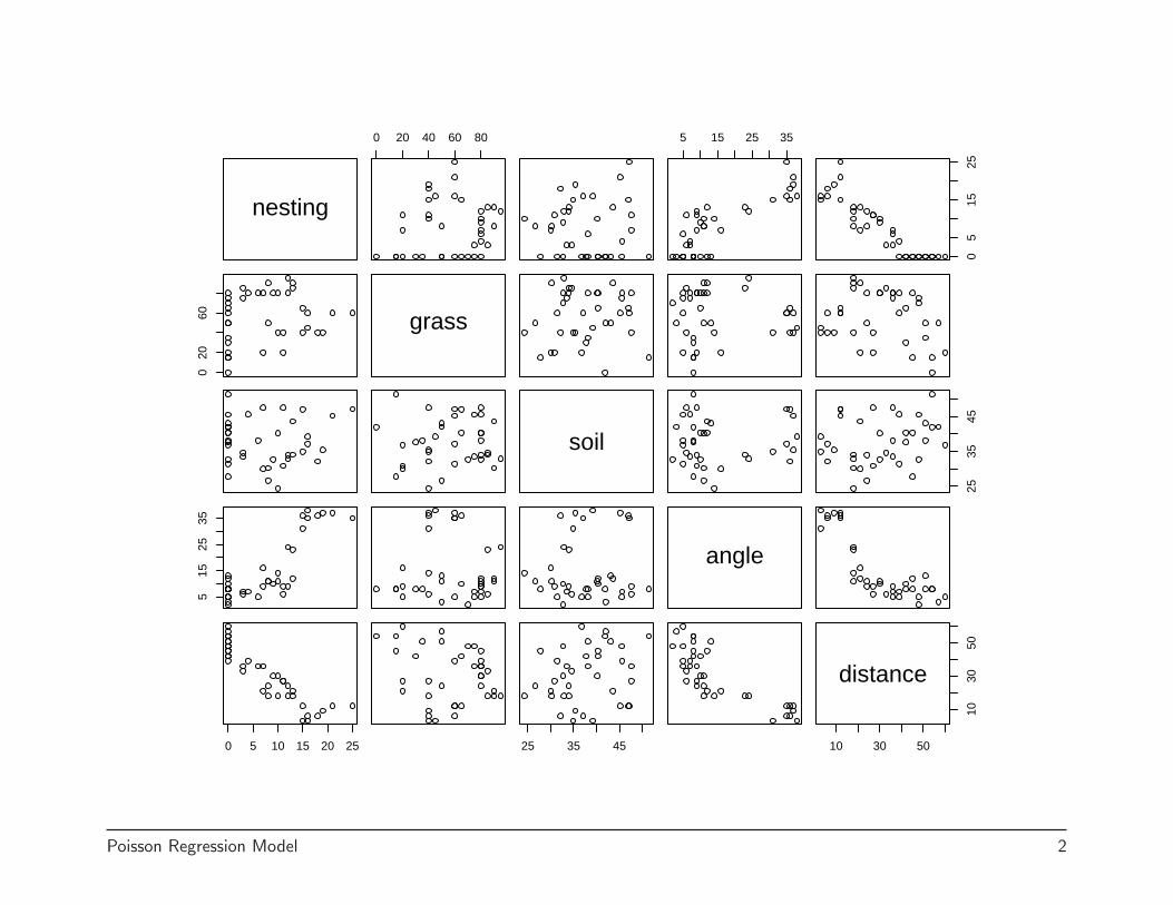
Four variables where considered in trying to describethe nesting frequency of the common puffin in a3m× 3m grid of plots.
• nesting: number of nests per 9m2
• grass: grass cover percentage
• soil: mean soil depth in cm
• angle: angle of slope in degrees
• distance: distance from cliff edge in m
Poisson Regression Model 1
nesting
0 20 40 60 80 5 15 25 35
05
1525
020
60 grass
soil
2535
45
515
2535
angle
0 5 10 15 20 25 25 35 45 10 30 50
1030
50
distance
Poisson Regression Model 2
Poisson Regression Model
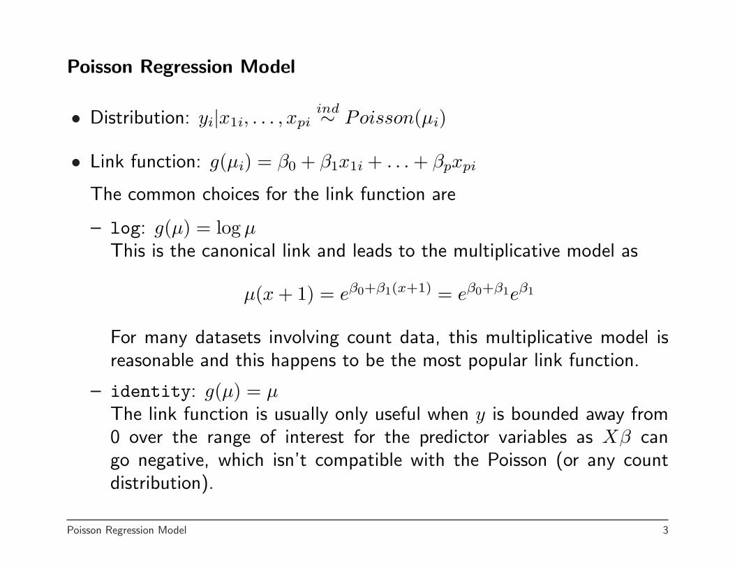
• Distribution: yi|x1i, . . . , xpiind∼ Poisson(µi)
• Link function: g(µi) = β0 + β1x1i + . . . + βpxpi
The common choices for the link function are
– log: g(µ) = log µThis is the canonical link and leads to the multiplicative model as
µ(x + 1) = eβ0+β1(x+1) = eβ0+β1eβ1
For many datasets involving count data, this multiplicative model isreasonable and this happens to be the most popular link function.
– identity: g(µ) = µThe link function is usually only useful when y is bounded away from0 over the range of interest for the predictor variables as Xβ cango negative, which isn’t compatible with the Poisson (or any countdistribution).
Poisson Regression Model 3

– sqrt (Square root): g(µ) =√
µThis is an analog to the variance stabilizing transformation which hasbeen used in the past. By the delta rule, if Var(Y |X) = E[Y |X] =µ(X),
Var(√
Y |X) ≈ 14
Note that for the the log and sqrt link functions, additive models onthe linear predictor scale lead to interactions on the mean scale.
For the log link,µ(x1, x2) = eβ0eβ1x1eβ2x2
In this case the effect of x1 depends on the level of x2 (and vice-versa).
Similarly, for the sqrt link
µ(x1, x2) = β20 + 2β0β1x1 + 2β0β2x2 + +2β1β1x1x2 + β2
1x21 + β2
2x22
• Variance function: V (µi) = µi
Poisson Regression Model 4

As we have seen before, this data can easily analyzed by
> puffin.glm <- glm(nesting ~ grass + soil + angle + distance,data=puffin, family=poisson())
> summary(puffin.glm)
Call:glm(formula = nesting ~ grass + soil + angle + distance,
family = poisson(), data = puffin)
Deviance Residuals:Min 1Q Median 3Q Max
-2.3263 -1.2984 -0.6617 0.8119 2.5304
Poisson Regression Model 5

Coefficients:Estimate Std. Error z value Pr(>|z|)
(Intercept) 3.069973 0.452568 6.783 1.17e-11 ***grass 0.005441 0.003104 1.753 0.07960 .soil 0.033441 0.010822 3.090 0.00200 **angle -0.030077 0.010724 -2.805 0.00504 **distance -0.089399 0.010680 -8.371 < 2e-16 ***---Signif. codes: 0 ’***’ 0.001 ’**’ 0.01 ’*’ 0.05 ’.’ 0.1 ’ ’ 1
(Dispersion parameter for poisson family taken to be 1)
Null deviance: 310.427 on 37 degrees of freedomResidual deviance: 68.765 on 33 degrees of freedomAIC: 183.38
Number of Fisher Scoring iterations: 6
Poisson Regression Model 6

> anova(puffin.glm)Analysis of Deviance Table
Model: poisson, link: log
Response: nesting
Terms added sequentially (first to last)
Df Deviance Resid. Df Resid. DevNULL 37 310.427grass 1 6.393 36 304.033soil 1 0.033 35 304.000angle 1 159.343 34 144.657distance 1 75.892 33 68.765
Poisson Regression Model 7

Inference in Poisson Regression
As with logistic regression, inference can be based on Wald procedures forconfidence intervals and tests on single βs and Likelihood Ratio drop indeviance tests on one or more parameters.
For example, an approximate confidence interval for βj is
β̂j ± z∗α/2SE(β̂j) = (L,U)
A confidence interval for eβj is given by
(eL, eU)
Inference in Poisson Regression 8

For example, for the effect of distance, 95% confidence intervals for β4
and eβ4 are
> betahat <- coef(puffin.glm)[5]> se <- sqrt(vcov(puffin.glm)[5,5])> cibeta <- c(betahat-qnorm(0.975)*se, betahat+qnorm(0.975)*se)> betahat
distance-0.08939925> cibeta
distance distance-0.11033098 -0.06846753> exp(betahat)distance0.9144804> exp(cibeta)distance distance0.8955377 0.9338238
Inference in Poisson Regression 9

In addition, we can get confidence intervals for mean responses by a similarapproach. The usual estimate of the mean response with predictor vectorX is
µ̂(X) = g−1(Xβ̂)
So for the log link, this is
µ̂(X) = eXβ̂
A confidence interval for g(µ(X)) is
Xβ̂ ± z∗α/2
√XV̂ar(β̂)XT = (L,U)
which is then transformed
(g−1(L), g−1(U))
to give a confidence interval for µ(X).
Inference in Poisson Regression 10

The basic components can be calculated in R with the predict function,using the type="link" option.
For independent observations, the log-likelihood is
l(β) =n∑
i=1
yi log µi − µi − log yi!
This gives a deviance for Poisson regression of
G2 = 2n∑
i=1
yi logyi
µ̂i− yi + µ̂i
(This is set so the saturated model has a deviance of 0.)
Inference in Poisson Regression 11
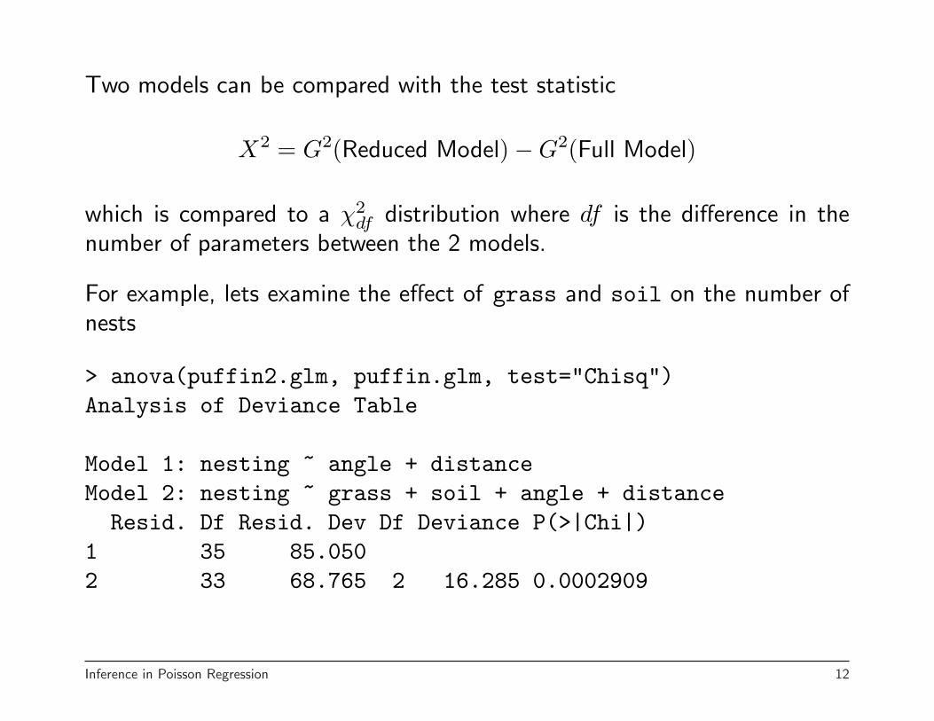
Two models can be compared with the test statistic
X2 = G2(Reduced Model)−G2(Full Model)
which is compared to a χ2df distribution where df is the difference in the
number of parameters between the 2 models.
For example, lets examine the effect of grass and soil on the number ofnests
> anova(puffin2.glm, puffin.glm, test="Chisq")Analysis of Deviance Table
Model 1: nesting ~ angle + distanceModel 2: nesting ~ grass + soil + angle + distanceResid. Df Resid. Dev Df Deviance P(>|Chi|)
1 35 85.0502 33 68.765 2 16.285 0.0002909
Inference in Poisson Regression 12
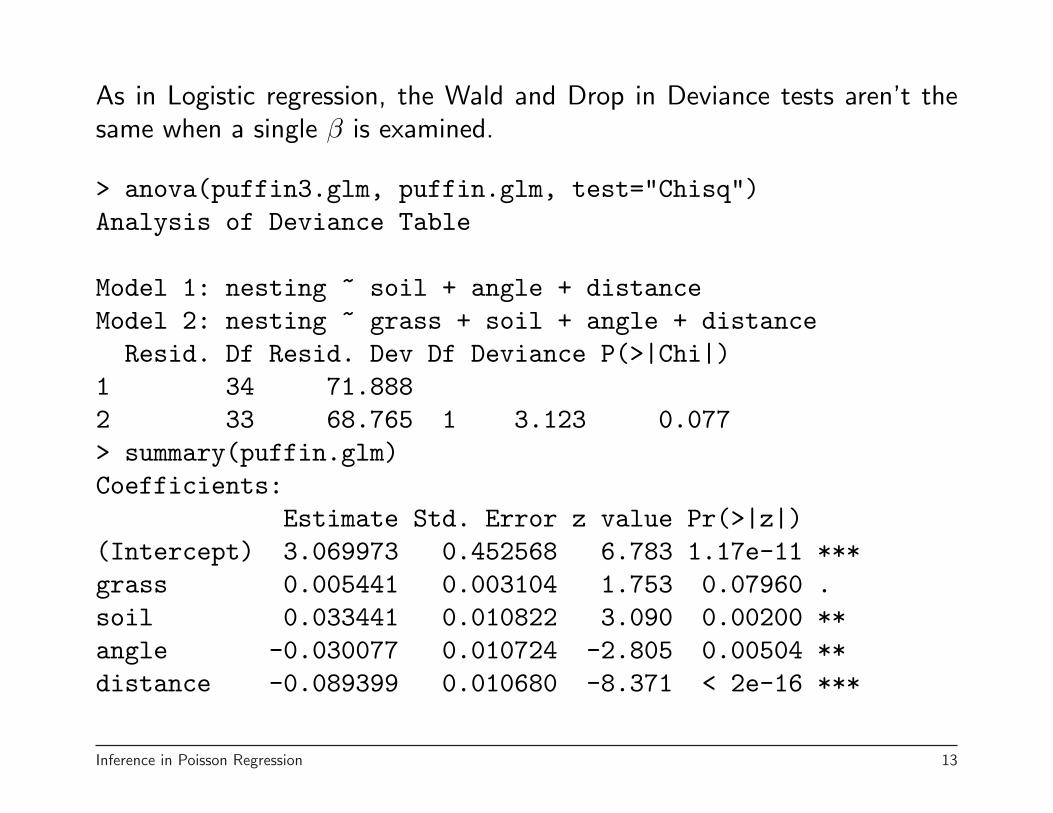
As in Logistic regression, the Wald and Drop in Deviance tests aren’t thesame when a single β is examined.
> anova(puffin3.glm, puffin.glm, test="Chisq")Analysis of Deviance Table
Model 1: nesting ~ soil + angle + distanceModel 2: nesting ~ grass + soil + angle + distanceResid. Df Resid. Dev Df Deviance P(>|Chi|)
1 34 71.8882 33 68.765 1 3.123 0.077> summary(puffin.glm)Coefficients:
Estimate Std. Error z value Pr(>|z|)(Intercept) 3.069973 0.452568 6.783 1.17e-11 ***grass 0.005441 0.003104 1.753 0.07960 .soil 0.033441 0.010822 3.090 0.00200 **angle -0.030077 0.010724 -2.805 0.00504 **distance -0.089399 0.010680 -8.371 < 2e-16 ***
Inference in Poisson Regression 13

Model Diagnostics
To examine the fit of the model, similar approaches are taken as in logisticregression. As before, there are two types of residuals used
• Deviance residual
Dresi = sign(Yi − µ̂i)
√2
[yi log
yi
µ̂i− yi + µ̂i
]
Note that the form of residual changes as deviance residuals depend onthe form of the log likelihood.
As before these can be calculated in R by resid(glm.object).
Inference in Poisson Regression 14

• Pearson residuals
Presi =Yi − µ̂i√
µ̂i
This is of a similar form as seen before, except for the change in theform of Var(Yi) that occurs in the denominator.
Note that it ends up that these can be easily gotten in Rby resid(glm.object, type="pearson"). This works for anygeneralized model, including logistic regression.
While usually not useful here, it is also possible to get the raw residualsyi− µ̂i in R with the command resid(glm.object, type="response").
Inference in Poisson Regression 15

0 5 10 15 20 25
−2
−1
01
2
Fitted Nests
Dev
ianc
e R
esid
uals
0 20 40 60 80
−2
−1
01
2
Grass Cover
Dev
ianc
e R
esid
uals
25 30 35 40 45 50
−2
−1
01
2
Soil
Dev
ianc
e R
esid
uals
0 5 10 15 20 25
−2
−1
01
23
Fitted Nests
Pea
rson
Res
idua
ls
0 20 40 60 80
−2
−1
01
23
Grass Cover
Pea
rson
Res
idua
ls
25 30 35 40 45 50
−2
−1
01
23
SoilP
ears
on R
esid
uals
Inference in Poisson Regression 16

5 10 15 20 25 30 35
−2
−1
01
2
Angle of Slope
Dev
ianc
e R
esid
uals
10 20 30 40 50 60
−2
−1
01
2
Distance from Cliff Edge
Dev
ianc
e R
esid
uals
5 10 15 20 25 30 35
−2
−1
01
23
Angle of Slope
Pea
rson
Res
idua
ls
10 20 30 40 50 60
−2
−1
01
23
Distance from Cliff Edge
Pea
rson
Res
idua
ls
Inference in Poisson Regression 17

These look pretty good. There is one observation that stands out, witha Pearson residual of 3. Interestingly, it doesn’t stand out strongly in thescatterplot matrix
> cbind(puffin,pear.resid, dev.resid, fitted(puffin.glm))[24,]nesting grass soil angle distance pear.resid dev.resid
24 11 20 30.8 9 27 2.990383 2.530391fitted(puffin.glm)
24 4.591954
If the underlying µi are large, both the deviance and Pearson residuals areapproximately N(0, 1) distributed. However if many of the µ̂i < 5, theusual normal based cutoffs are questionable.
Not surprisingly, it is also possible to perform Goodness of Fit tests forPoisson data.
Inference in Poisson Regression 18

• Deviance Goodness of Fit test:
X2 = 2n∑
i=1
yi logyi
µ̂i− yi + µ̂i
=n∑
i=1
Dres2i = G2
This is compared to a χ2n−p distribution.
The information for this test is given in the summary of the glm. For theexample,
> summary(puffin.glm)
Null deviance: 310.427 on 37 degrees of freedomResidual deviance: 68.765 on 33 degrees of freedom
Inference in Poisson Regression 19

> pchisq(deviance(puffin.glm), df.residual(puffin.glm),lower.tail=F)
[1] 0.0002572599
• Pearson Goodness of Fit test:
X2p =
n∑
i=1
(Yi − µ̂i)2
µ̂i
=n∑
i=1
Pres2i
Similarly, it is also compared to a χ2n−p distribution.
> pchisq(sum(pear.resid^2), df.residual(puffin.glm),lower.tail=F)
[1] 0.006662672
Inference in Poisson Regression 20

Small p-values for these tests can be caused by many things, including
• Incorrect mean model, e.g. missing predictors
• Poisson model is wrong. For example, maybe Var(Y |X) > µ(Y |X).
• Outliers contaminating the data
As with binomial data, these tests break down if there many observationswith small Poisson means (e.g. µ̂i < 5).
In cases like this, such as the example, other tools for examining the fit,such as testing extra terms (e.g. βx2), should be used.
Inference in Poisson Regression 21

It is also possible to examine for influence using similar approaches as before.For this example, not much stands out, except for one observation that has
large leverage(> 3
√p
n−p
).
dfb.1 dfb.gr dfb.so dfb.ang dfb.dst dffit cov.r cook.d hat5 0.068 -0.192 0.253 -0.2490 -0.1667 0.332 2.19 2.3e-02 0.478
> cbind(puffin,pear.resid, dev.resid, fitted(puffin.glm))[5,]nesting grass soil angle distance pear.resid dev.resid
5 11 40 47.6 6 27 0.3740736 0.3669813fitted(puffin.glm)
5 9.827332
Inference in Poisson Regression 22

Offsets
Often with count data, the expected counts will depend on an observationtime, or an observation area. The idea being, if you observe for twice aslong, you expect the count to double. So often the mean model will looklike
µi = ti × ri
where ti is observation time (or equivalent) and ri is the rate (expectedcount per observation unit).
The log-linear model works well in this situation as
log µi = log(tiri)
= log ti + log ri
= log ti + β0 + β1xi1 + . . . + βpxip
The quantity log ti is often referred to as the offset.
Offsets 23

Wave Damage to Cargo Ships: Data was collected by Lloyd’s Register ofShipping investigating the damage caused by waves to the forward sectionof certain cargo-carrying vessels. Three factors are believed to affect thenumber of damage incidents
• Ship type: A - E
• Year of construction: 1960-64, 1965-69, 1970-74, 1975-1979
• Period of operation: 1960-74, 1975-1979
The observation times varied greatly (45 to 44882 months) and thus mustbe taken account of in the analysis. For example
Offsets 24

Ship Year of Period of Aggregate Damage Damage Rate
Type Construction Operation Service Time Damage (per 1000 months)
B 1960-64 1960-74 44882 39 0.869
B 1960-64 1975-79 17176 29 1.688
B 1965-69 1960-74 28609 58 2.027
B 1965-69 1975-79 20370 53 2.602
A B C D E
05
1015
Ship Type
Dam
age
Rat
es (
per
1000
mon
ths)
1960−64 1970−74
05
1015
Construction Year
Dam
age
Rat
es (
per
1000
mon
ths)
1960−74 1975−790
510
15Operation Period
Dam
age
Rat
es (
per
1000
mon
ths)
Offsets 25

Lets examining the model
log µ = β0 + β1Type + β2Construct + β3Operation + log Service
This can be done in R by using the offset option to glm.
> wave.glm <- glm(Damage ~ Type + Construct + Operation,offset=log(Service), data=wave2, family=poisson())
> summary(wave.glm)
Call:glm(formula = Damage ~ Type + Construct + Operation,
family = poisson(), data = wave2, offset = log(Service))
Deviance Residuals:Min 1Q Median 3Q Max
-1.6768 -0.8293 -0.4370 0.5058 2.7912
Offsets 26

Coefficients:Estimate Std. Error z value Pr(>|z|)
(Intercept) -6.40590 0.21744 -29.460 < 2e-16 ***TypeB -0.54334 0.17759 -3.060 0.00222 **TypeC -0.68740 0.32904 -2.089 0.03670 *TypeD -0.07596 0.29058 -0.261 0.79377TypeE 0.32558 0.23588 1.380 0.16750Construct1965-69 0.69714 0.14964 4.659 3.18e-06 ***Construct1970-74 0.81843 0.16977 4.821 1.43e-06 ***Construct1975-79 0.45343 0.23317 1.945 0.05182 .Operation1975-79 0.38447 0.11827 3.251 0.00115 **---Signif. codes: 0 ’***’ 0.001 ’**’ 0.01 ’*’ 0.05 ’.’ 0.1 ’ ’ 1
(Dispersion parameter for poisson family taken to be 1)
Null deviance: 146.328 on 33 degrees of freedomResidual deviance: 38.695 on 25 degrees of freedomAIC: 154.56
Offsets 27

In this example, all three factors seem to be important as
> anova(wave.t.glm, wave.glm, test="Chisq")Analysis of Deviance Table
Model 1: Damage ~ Construct + OperationModel 2: Damage ~ Type + Construct + OperationResid. Df Resid. Dev Df Deviance P(>|Chi|)
1 29 62.3652 25 38.695 4 23.670 9.3e-05
> anova(wave.c.glm, wave.glm, test="Chisq")Analysis of Deviance Table
Model 1: Damage ~ Type + OperationModel 2: Damage ~ Type + Construct + OperationResid. Df Resid. Dev Df Deviance P(>|Chi|)
1 28 70.1032 25 38.695 3 31.408 6.975e-07
Offsets 28

> anova(wave.o.glm, wave.glm, test="Chisq")Analysis of Deviance Table
Model 1: Damage ~ Type + ConstructModel 2: Damage ~ Type + Construct + OperationResid. Df Resid. Dev Df Deviance P(>|Chi|)
1 26 49.3552 25 38.695 1 10.660 0.001
This should be taken with some grain of salt as it appears that there is abit of a problem with the model.
Offsets 29
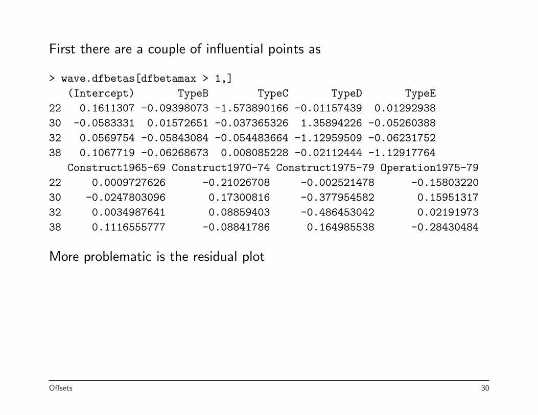
First there are a couple of influential points as
> wave.dfbetas[dfbetamax > 1,](Intercept) TypeB TypeC TypeD TypeE
22 0.1611307 -0.09398073 -1.573890166 -0.01157439 0.0129293830 -0.0583331 0.01572651 -0.037365326 1.35894226 -0.0526038832 0.0569754 -0.05843084 -0.054483664 -1.12959509 -0.0623175238 0.1067719 -0.06268673 0.008085228 -0.02112444 -1.12917764
Construct1965-69 Construct1970-74 Construct1975-79 Operation1975-7922 0.0009727626 -0.21026708 -0.002521478 -0.1580322030 -0.0247803096 0.17300816 -0.377954582 0.1595131732 0.0034987641 0.08859403 -0.486453042 0.0219197338 0.1116555777 -0.08841786 0.164985538 -0.28430484
More problematic is the residual plot
Offsets 30

0 10 20 30 40 50
−1
01
2
Fitted Damage Incidents
Dev
ianc
e R
esid
ual
A B C D E
−1
01
2
Ship Type
Dev
ianc
e R
esid
ual
1960−64 1965−69 1970−74 1975−79
−1
01
2
Construction Year
Dev
ianc
e R
esid
ual
1960−74 1975−79
−1
01
2
Operation Period
Dev
ianc
e R
esid
ual
Offsets 31


