
1
Recent Advances in Nonlinear Response Structural Optimization Using the Equivalent Static Loads
Method
Oct. 28, 2014 VR&D 2014 Users Conference
Monterey, CA
Gyung-Jin Park Professor, Hanyang University
Ansan City, Korea
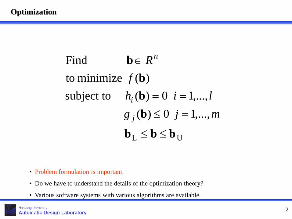
Optimization
2
• Problem formulation is important.
• Do we have to understand the details of the optimization theory?
• Various software systems with various algorithms are available.
UL
,...,10)(,...,10)( subject to
)( minimize toFind
bbb
bbb
b
≤≤
=≤==
∈
mjglih
fR
j
i
n

Linear Static Response Structural Optimization
3
• Popular
• Easy
• Well developed software systems are available.
UL
,...,10),()(: subject to
),( minimize to,Find
bbb
zbfzbKh
zbzb
≤≤
=≤=
∈∈
mjg
fRR
j
ln
Linear Static Response Structural Optimization
4
• Size Optimization: The FEM data are fixed.
• Shape Optimization: Node and element data of FEM analysis are changed
during optimization.
• Topology Optimization: Material distribution is optimized.
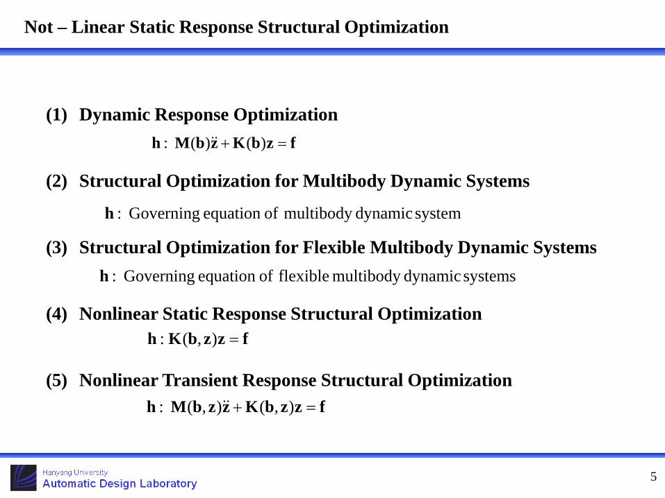
Not – Linear Static Response Structural Optimization
5
(1) Dynamic Response Optimization
(2) Structural Optimization for Multibody Dynamic Systems
(3) Structural Optimization for Flexible Multibody Dynamic Systems
(4) Nonlinear Static Response Structural Optimization
(5) Nonlinear Transient Response Structural Optimization
fzbKzbMh =+ )()(:
fzzbKh =),(:
system dynamicmultibody ofequation Governing:h
fzzbKzzbMh =+ ),(),(:
systems dynamicmultibody flexible ofequation Governing:h

The Equivalent Static Loads Method
6
Not a Linear Response Analysis
Linear Static Optimization
Disp. Field
Multiple Loading Conditions
Equivalent Static Loads
Updated design
Analysis Domain Design Domain
• This method has been developed for not-linear static response structural optimization.
• Analysis is performed in the analysis domain.
• Equivalent loads are calculated.
• Linear response optimization is performed using the equivalent static loads in the design domain.
• The process proceeds in a cyclic manner.

Contents
7
(1) Linear Dynamic Response Optimization
(2) Structural Optimization for Multibody Dynamic Systems
(3) Structural Optimization for Flexible Multibody Dynamic Systems
(4) Nonlinear Static Response Structural Optimization
(5) Nonlinear Transient Response Structural Optimization

8
Nonlinear Static Response
Optimization Using Equivalent Loads
(NROEL) – Installed in NASTRAN

Nonlinear Response Optimization
9
General Formulation
,m,ig
f
i 1;0)()(subject to)(minimize to
Find
=≤=
zb,fzzb,K
zb,b
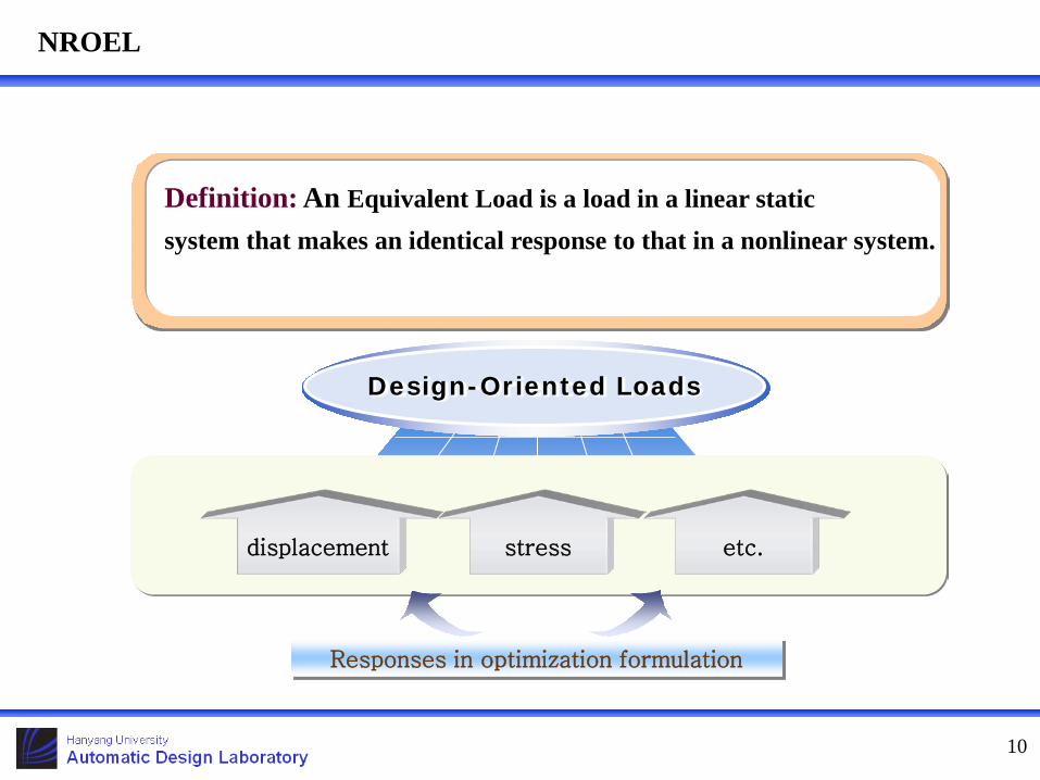
NROEL
10
Definition: An Equivalent Load is a load in a linear static system that makes an identical response to that in a nonlinear system.
Design-Oriented Loads
displacement stress etc.
Responses in optimization formulation

Flow of NROEL
11
START
? No
Nonlinear Analysis fzzb,K =NN )(
Calculate Equivalent Loads
NLeq zKf =
Update Design
Linear Response Optimization
,m,ig
f
Li
eqLL
L
1;0)()(subject to
)(minimize toFind
=≤
=
zb,fzbK
zb,b
END
Optimization process using equivalent loads
ε≤− − )1()( keq
keq ff
k=0 k=k+1
The one for stress constraints is separately defined.

Shape Optimization 1
12
11.22E+6 N
b1
Geometric and Material Nonlinearity -Linear hardening
E = 200.0 GPa σy = 300.0 Mpa Eh = 50.0 GPa
Shape change – using domain element
2. A plate
Nonlinear Response Optimization
2001;00.1.350/)(subject to
Massminimize tochange) shape(Find 321
,,j
, b, bb
j
NN
=≤−=
σfzzb,K
b2
b3
b1
b2 b3
<D.V. and perturbation of the shape >
<Applied loads and boundary conditions>

Shape Optimization 1
13
Results of Optimization Initial design
Conventional method
NROESL Initial design
Con. Meth. (215)
NROEL (7)
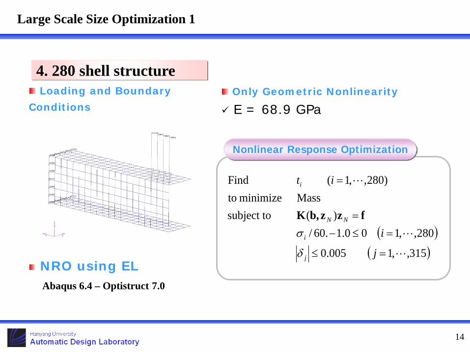
Large Scale Size Optimization 1
14
Only Geometric Nonlinearity E = 68.9 GPa
Loading and Boundary Conditions
4. 280 shell structure
Nonlinear Response Optimization
( )( )315,,1005.0
280,,100.1.60/)(subject to
Massminimize to)280,,1(Find
=≤
=≤−=
=
j
i
it
j
i
NN
i
δ
σfzzb,K
NRO using EL Abaqus 6.4 – Optistruct 7.0

Large Scale Size Optimization 1
15
Results of Optimization
< Design history graph > < Optimum thickness contour >
Optimization using the conventional method is fairly expensive.

0.5kN 0.5kN
0.5kN 0.5kN
16
Shape Optimization with Linear Contact
6. A Ring: Problem Definition
Problem model
- Loading condition: The forces are applied at the elements of the upper parts.
- The element property: PSOLID
- The total number of elements: 672 ( 64 CPENTA + 608 CHEXA)
- Only the boundary nonlinearity is considered.
- NASTRAN is used for contact analysis and linear response optimization.
- NASTRAN DMAP is utilized for calculating the equivalent loads.
Solver: SOL 101
- Linear contact: Linear analysis + Nonlinear contact parameters
cΓcontact boundaries ( )

17
Design condition
Design perturbation vectors
- Perturbation vectors are utilized for shape change in shape optimization.
- Each arrow is a perturbation vector.
- Seven design variables are selected based on the perturbation vectors.
Shape Optimization with Linear Contact
b1
b2 b2
b1 b3 b3
b4 b4
b5 b5
b6 b6
b7
)672,,1(0KPa0.2subject tomassmin. to
ring) theof(shape,,,Find 721
=≤− i
bbb
iσ
Formulation
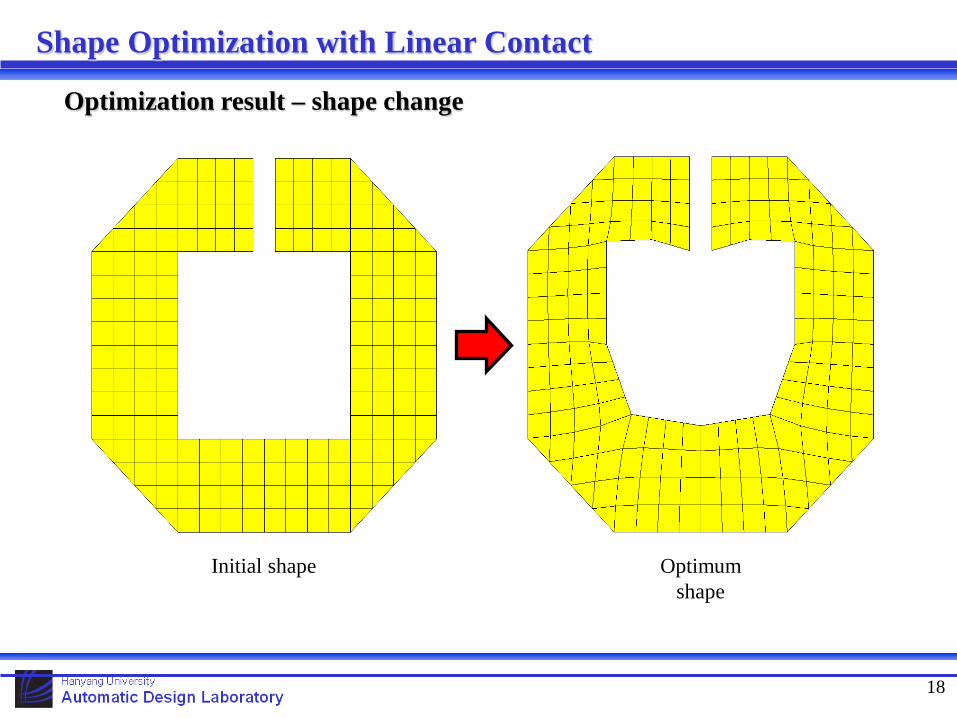
18
Optimization result – shape change
Shape Optimization with Linear Contact
Initial shape Optimum shape

19
Nonlinear Dynamic Response Optimization Using Equivalent Static
Loads – Installed in GENESIS and OptiStruct
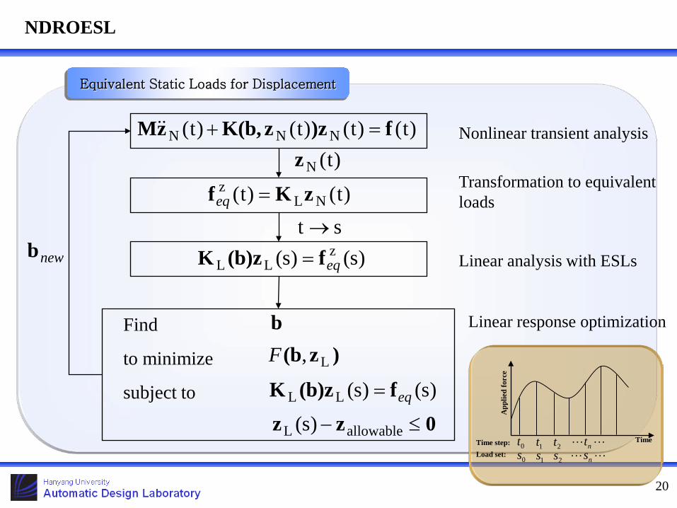
NDROESL
20
Equivalent Static Loads for Displacement
App
lied
forc
e
Time Time step: Load set:
0t 1t 2t nt0s 1s 2s ns
)t()t()t()t( NNN f)zzK(b,zM =+
)t()t( NLz zKf =eq
)s()s( zLL eqf(b)zK =
Nonlinear transient analysis
Transformation to equivalent loads
Linear analysis with ESLs
Linear response optimization
)t(Nz
st →
Find
to minimize
subject to
0zz ≤− allowableL )s(
b)z(b L,F
)s()s(LL eqf(b)zK =
newb

Flow of NDROESL
21
START
? No
Nonlinear Dynamic Analysis
)()()( tt(t) NNN fzzb,KzM(b) =+
Calculate Equivalent Static Loads
)()( tt NLeq zKf =
Update Design
Linear Response Optimization
,m,igqttt
f
Li
eqLL
L
1;0)(
,,1);()()(subject to)(minimize to
Find
=≤
==
zb,fzbK
zb,b
END
Optimization process using equivalent static loads
ε≤− − )1()( keq
keq ff
k=0 k=k+1
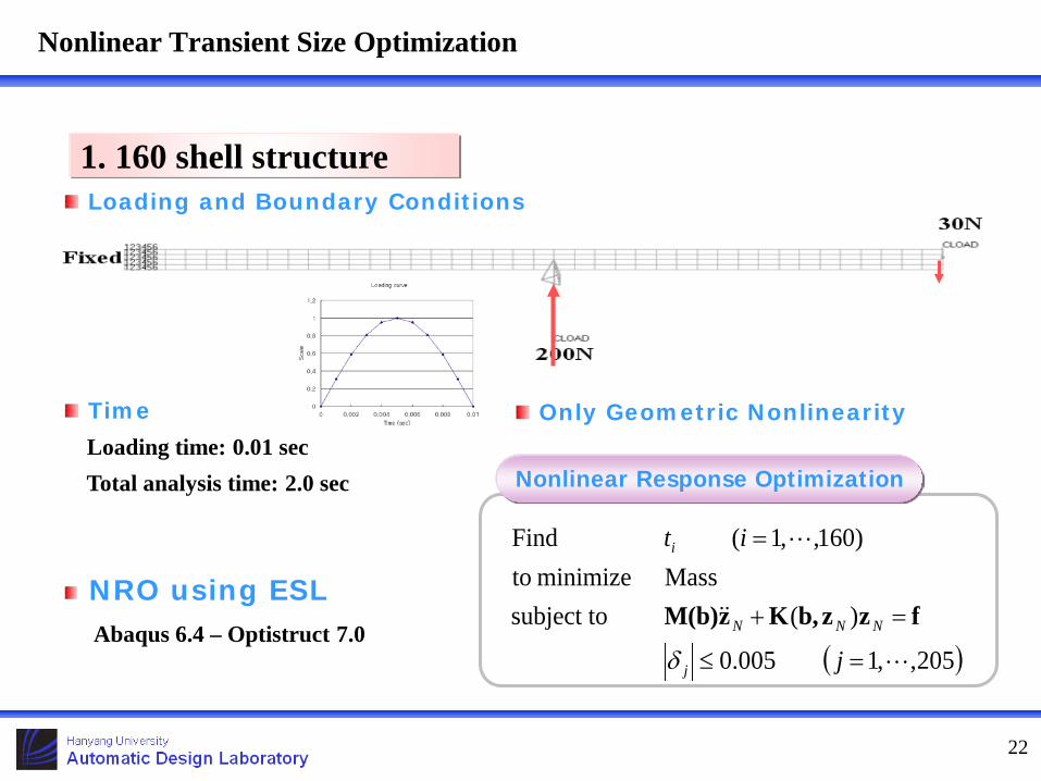
Nonlinear Transient Size Optimization
22
Loading and Boundary Conditions
1. 160 shell structure
Nonlinear Response Optimization
( )205,,1005.0
)(subject toMassminimize to
)160,,1(Find
=≤
=+
=
j
it
j
NNN
i
δ
fzzb,KzM(b) NRO using ESL
Abaqus 6.4 – Optistruct 7.0
Time Loading time: 0.01 sec Total analysis time: 2.0 sec
Only Geometric Nonlinearity

Nonlinear Transient Size Optimization
23
Results of Optimization
< Design history graph >
< Optimum thickness contour >
Initial
Optimum
< Tip displacement >
Roof Crush Optimization
24
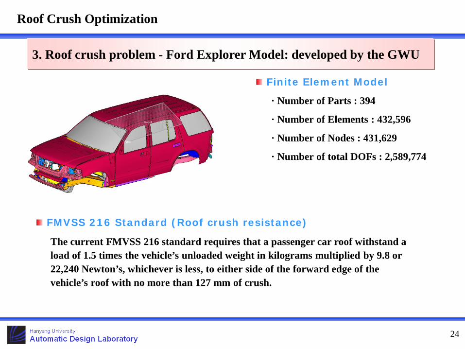
3. Roof crush problem - Ford Explorer Model: developed by the GWU
Finite Element Model
· Number of Parts : 394
· Number of Elements : 432,596
· Number of Nodes : 431,629
· Number of total DOFs : 2,589,774
FMVSS 216 Standard (Roof crush resistance)
The current FMVSS 216 standard requires that a passenger car roof withstand a load of 1.5 times the vehicle’s unloaded weight in kilograms multiplied by 9.8 or 22,240 Newton’s, whichever is less, to either side of the forward edge of the vehicle’s roof with no more than 127 mm of crush.

25
Roof Crush Optimization
Definition of design variables
DV 1: Thickness of A-Pillar (t1)
DV 2: Thickness of B-Pillar (t2)
DV 3: Thickness of Roof-Rail (t3)
< Roof Structure >
DV 1
DV 3
DV 2

26
Roof Crush Optimization
0.23dv6.0.022dv.60.021dv.60
67.5ms)(t 0.0 crush roof theof distance127mm)(subject to
massminimize to )3,2,1(Find
step
≤≤≤≤≤≤
=≤−=+
=
fzzb,KzM(b) NNN
i it
Modify
Modified formulation for the ESL method
.023dv6.0.022dv.60.021dv.60
127mm) crush (roof 0.0forcewallrigidweight1.65)(subject to
massminimize to)3,2,1(Find
≤≤≤≤≤≤
=≥−×=+
=
fzzb,KzM(b) NNN
i it
Roof Crush Optimization Using RSM and ESL
27
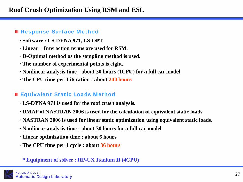
Response Surface Method · Software : LS-DYNA 971, LS-OPT · Linear + Interaction terms are used for RSM. · D-Optimal method as the sampling method is used. · The number of experimental points is eight. · Nonlinear analysis time : about 30 hours (1CPU) for a full car model · The CPU time per 1 iteration : about 240 hours
· LS-DYNA 971 is used for the roof crush analysis. · DMAP of NASTRAN 2006 is used for the calculation of equivalent static loads. · NASTRAN 2006 is used for linear static optimization using equivalent static loads. · Nonlinear analysis time : about 30 hours for a full car model · Linear optimization time : about 6 hours · The CPU time per 1 cycle : about 36 hours
Equivalent Static Loads Method
* Equipment of solver : HP-UX Itanium II (4CPU)

28
Results
4 Number of iterations
0.6 mm 0.6 mm 1.0 mm DV 3
3.329 kg 3.346 kg 4.481 kg Mass
5 33 Number of nonlinear analyses
5 Number of cycles
0.96 mm 0.6 mm 1.1 mm DV 2 0.86 mm 1.16 mm 1.2 mm DV 1
ESL result RSM result Initial model
+0.7% -11.2% Constraint violation
Roof Crush Optimization Using RSM and ESL
Total CPU time (1CPU) 990 hours 180 hours

29
Nonlinear Dynamic Response Topology Optimization Using the
Equivalent Static Loads
30
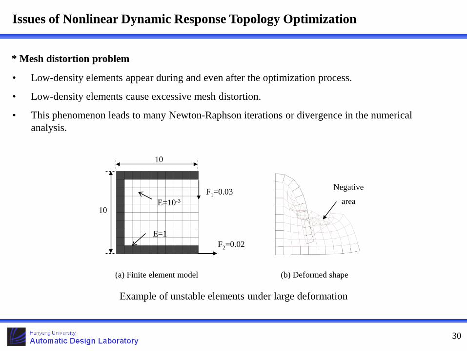
Issues of Nonlinear Dynamic Response Topology Optimization
Example of unstable elements under large deformation
• Low-density elements appear during and even after the optimization process.
• Low-density elements cause excessive mesh distortion.
• This phenomenon leads to many Newton-Raphson iterations or divergence in the numerical analysis.
F1=0.03
F2=0.02 E=1
E=10-3
10
10
Negative
area
(a) Finite element model (b) Deformed shape
* Mesh distortion problem

31
Issues of Nonlinear Dynamic Response Topology Optimization
• The purpose of topology optimization
Maximization of the stiffness of the structure = Minimization of the compliance
• The general objective function for linear topology optimization fTz
• When topology optimization in the time domain is performed, the objective functions are as follows:
1) The weighted summation compliance
2) The weighted summation compliance near the peaks
* Definition of the objective function
( ) luωl
uuuu ...,,1=;∑
1=
Tzf
( ) puωp
uuuu ...,,1=;∑
1=
Tzf : the number of time steps in the time domain
: the weighting factor
: the magnitude of the dynamic load vector at the uth time step
: the displacement vector of the uth time step
: the number of time steps near the peaks
p
ωl
u
u
u
zf

32
ESLSO
* ESLSO for nonlinear dynamic response topology optimization
)(=)())(,(+)()(+)()(
NNN
NN
ttttt
fzzbKzbCzbM
Nonlinear dynamic analysis
)()(=)( NL tseq zbKfCalculate ESLs
( )
1≤≤<0
≤
)(=)()(s.t.
min. to
...,,1=;Find
min
1=
LL
1=
T
∑
∑
i
n
iii
eq
p
uuuu
i
bb
Vbv
uu
ω
nib
fzbK
zf
Linear topology optimization
Transform into transformation variables
Start End
Update design
( ) 32)1()(countif εεαα ×− − nk
ik
i ≤≥
k=k+1
No
Yes
>≤
=1
1
when1when0
εε
αi
ii b
b
33
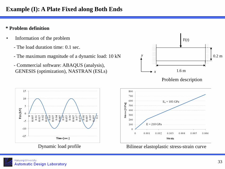
Example (I): A Plate Fixed along Both Ends
* Problem definition
• Information of the problem
- The load duration time: 0.1 sec.
- The maximum magnitude of a dynamic load: 10 kN
- Commercial software: ABAQUS (analysis), GENESIS (optimization), NASTRAN (ESLs) 1.6 m
0.2 m
x
y
F(t)
Problem description
Dynamic load profile Bilinear elastoplastic stress-strain curve
E = 210 GPa
Eh = 105 GPa
34
Example (I): A Plate Fixed along Both Ends
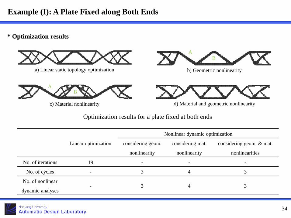
* Optimization results
Linear optimization
Nonlinear dynamic optimization
considering geom.
nonlinearity
considering mat.
nonlinearity
considering geom. & mat.
nonlinearities
No. of iterations 19 - - -
No. of cycles - 3 4 3
No. of nonlinear
dynamic analyses - 3 4 3
Optimization results for a plate fixed at both ends
a) Linear static topology optimization
c) Material nonlinearity
b) Geometric nonlinearity
d) Material and geometric nonlinearity
A B
B A
35
Example (II): A Crash Box for Crashworthiness
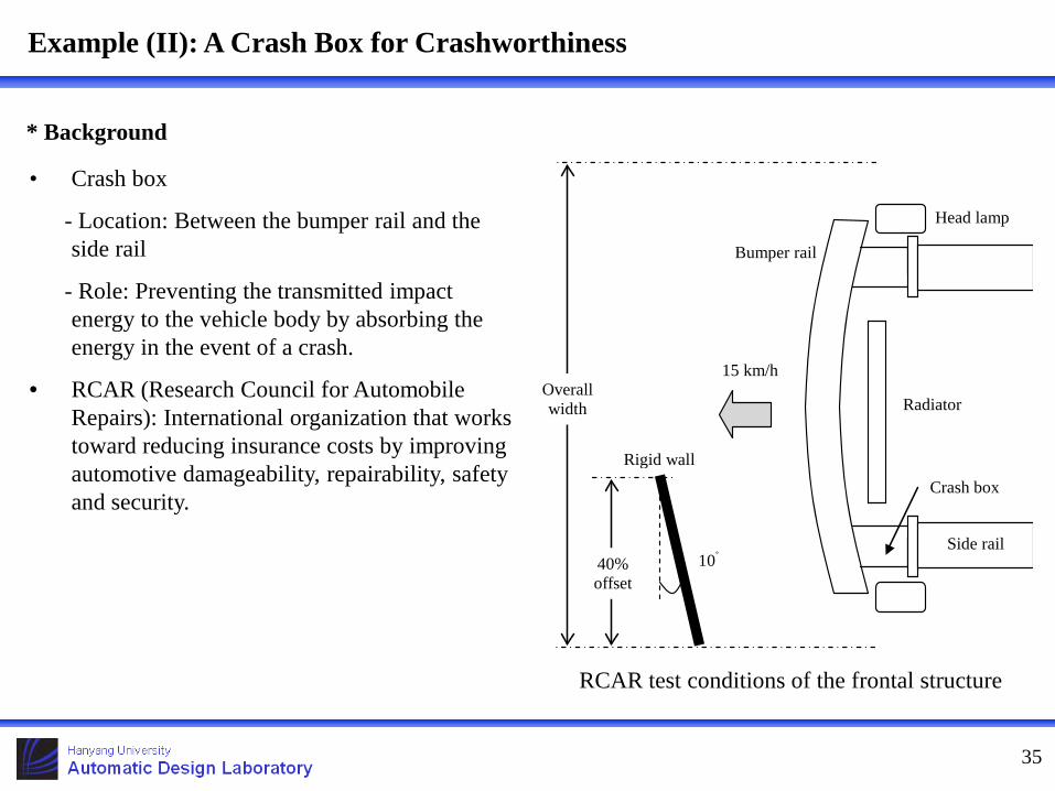
* Background
• Crash box
- Location: Between the bumper rail and the side rail
- Role: Preventing the transmitted impact energy to the vehicle body by absorbing the energy in the event of a crash.
• RCAR (Research Council for Automobile Repairs): International organization that works toward reducing insurance costs by improving automotive damageability, repairability, safety and security.
Radiator
Bumper rail
Side rail
Crash box
Rigid wall
15 km/h
40% offset
Overall width
Head lamp
10˚
RCAR test conditions of the frontal structure
36
Example (II): A Crash Box for Crashworthiness
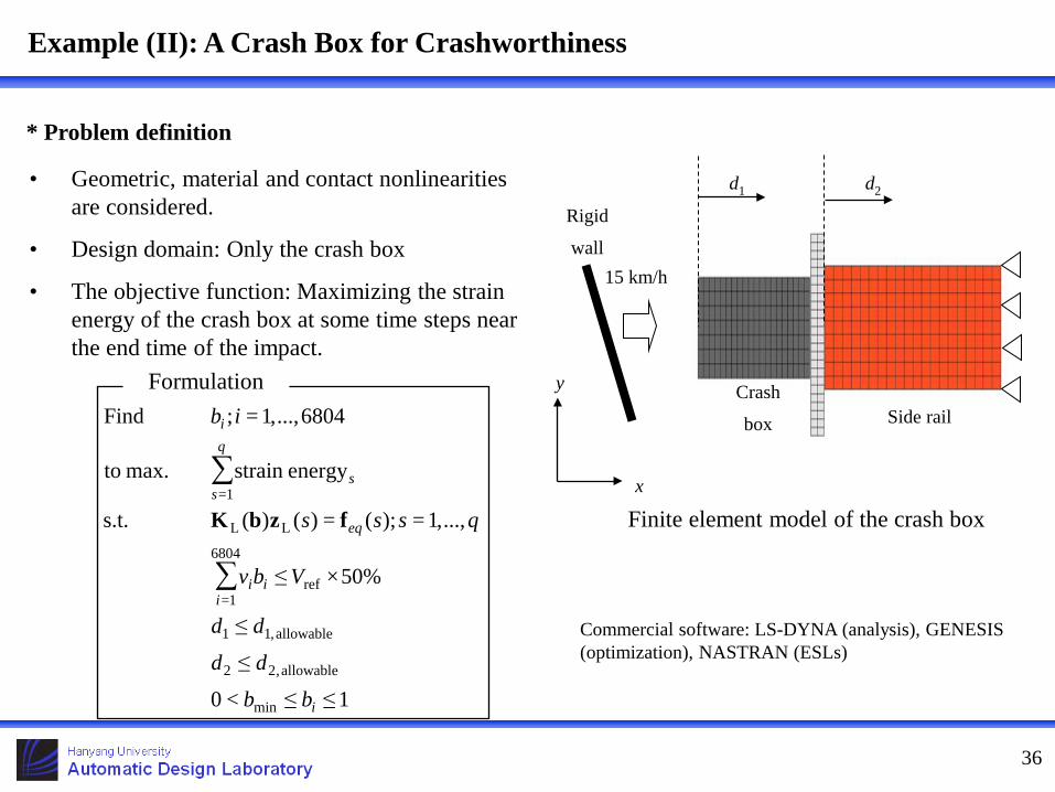
* Problem definition
• Geometric, material and contact nonlinearities are considered.
• Design domain: Only the crash box
• The objective function: Maximizing the strain energy of the crash box at some time steps near the end time of the impact.
Side rail Crash
box
x
y
15 km/h
Rigid
wall
d1 d2
Commercial software: LS-DYNA (analysis), GENESIS (optimization), NASTRAN (ESLs)
Finite element model of the crash box
1≤≤<0
≤
≤
%50×≤
...,,1=);(=)()(s.t.
energystrain max. to
6804...,,1=;Find
min
allowable,22
allowable,11
6804
1=ref
LL
1=
∑
∑
i
iii
eq
q
ss
i
bb
dd
dd
Vbv
qsss
ib
fzbK
Formulation
37
Example (II): A Crash Box for Crashworthiness
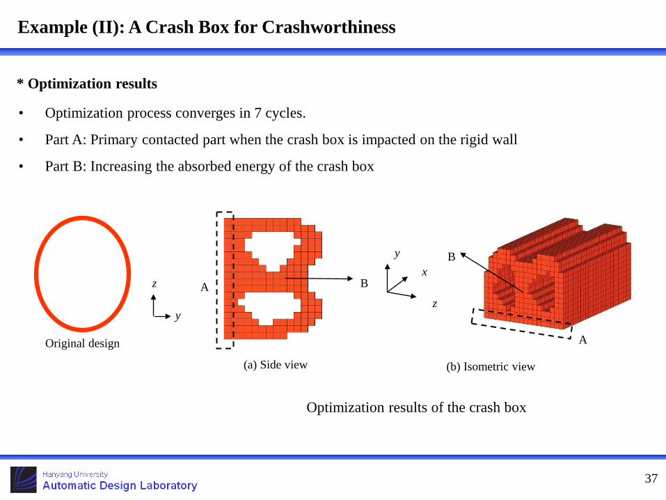
* Optimization results
• Optimization process converges in 7 cycles.
• Part A: Primary contacted part when the crash box is impacted on the rigid wall
• Part B: Increasing the absorbed energy of the crash box
y
z
x
(b) Isometric view
A
B
y
z A B
(a) Side view
Optimization results of the crash box
Original design

38
Sheet Metal Forming with a Tapered Square Cup
Geometric description of the tooling for the oblique square cup
• The tooling: the die, the punch and the blank holder • Blank holding force: 100 kN • Stroke of the punch: 40 mm (-z direction) • Wrinkling occurrence part: the side-wall • Reason of wrinkling occurrence at the side-wall - The geometry of the wall is not constrained by the die and the punch.
x
y
Die
114.3
Punch
R31.75
R50.8
152.4
y
z R6.35
R6.35
Punch
Die
Blank holder
Blank
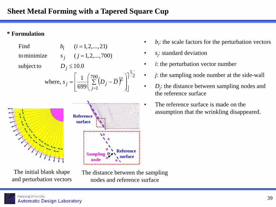
* Formulation
0.10tosubject
)700...,,2,1(minimizeto)21...,,2,1(Find
≤
==
j
j
i
D
jsib
• bi: the scale factors for the perturbation vectors
• sj: standard deviation
• i: the perturbation vector number
• j: the sampling node number at the side-wall
• Dj: the distance between sampling nodes and the reference surface
• The reference surface is made on the assumption that the wrinkling disappeared.
( )2
1700
1
26991,where
∑ −==j
jj DDs
The initial blank shape and perturbation vectors
Reference surface
Sampling node
D Reference
surface
The distance between the sampling nodes and reference surface
Sheet Metal Forming with a Tapered Square Cup
39

* Results
• The ranges of each design variable are changed after the second cycle.
• The move limit strategy is used.
• Objective function: 0.4781 0.2741 (convergence criteria: 2.0%)
Sheet Metal Forming with a Tapered Square Cup
40

* Results
Shape of blank after the sheet metal
forming
Split plane – height 20 mm Standard deviation Clip (+) Clip (-)
Initial model
0.4781
Optimum model
0.2741
x y
x y
x y
x y
y z
x
y z
x
Sheet Metal Forming with a Tapered Square Cup
41
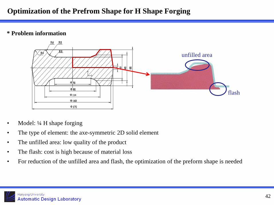
Optimization of the Prefrom Shape for H Shape Forging
42
* Problem information
unfilled area
flash
• Model: ¼ H shape forging • The type of element: the axe-symmetric 2D solid element • The unfilled area: low quality of the product • The flash: cost is high because of material loss • For reduction of the unfilled area and flash, the optimization of the preform shape is needed
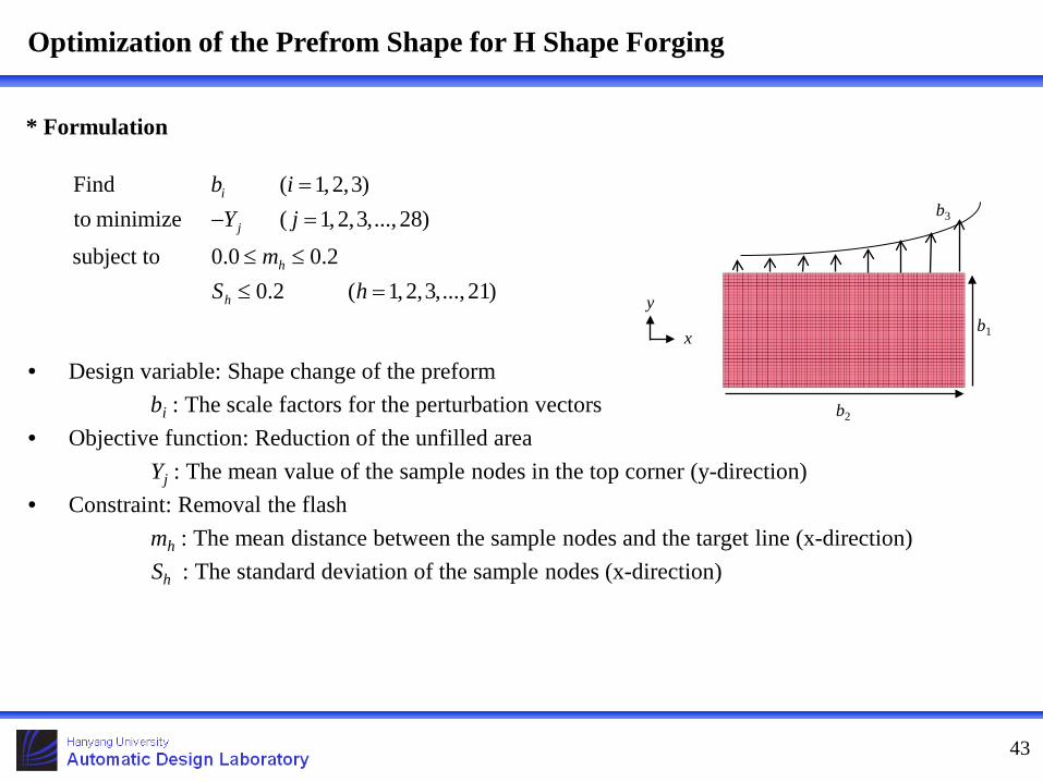
43
* Formulation
• Design variable: Shape change of the preform bi : The scale factors for the perturbation vectors • Objective function: Reduction of the unfilled area
Yj : The mean value of the sample nodes in the top corner (y-direction) • Constraint: Removal the flash
mh : The mean distance between the sample nodes and the target line (x-direction) Sh : The standard deviation of the sample nodes (x-direction)
)21...,,3,2,1(2.02.00.0subject to
)28...,,3,2,1(minimize to)3,2,1(Find
=≤≤≤
=−=
hSm
jYib
h
h
j
i
b1
b3
x
y
b2
Optimization of the Prefrom Shape for H Shape Forging

44
* Result
• Objective function: -32.892 -33.925
• Constraint violation: 175.4% 0%
• Number of cycles: 30
0
0.2
0.4
0.6
0.8
1
1.2
1.4
1.6
-34.0-33.8-33.6-33.4-33.2-33.0-32.8-32.6-32.4-32.2
0 2 4 6 8 10 12 14 16 18 20 22 24 26 28
Infin
ite n
orm
Obj
ectiv
e fu
nctio
n .
Cycle number
History of the objective function and the infinite norm of the design variable variation vector
Objective function Infinite norm of the design variable variation vector
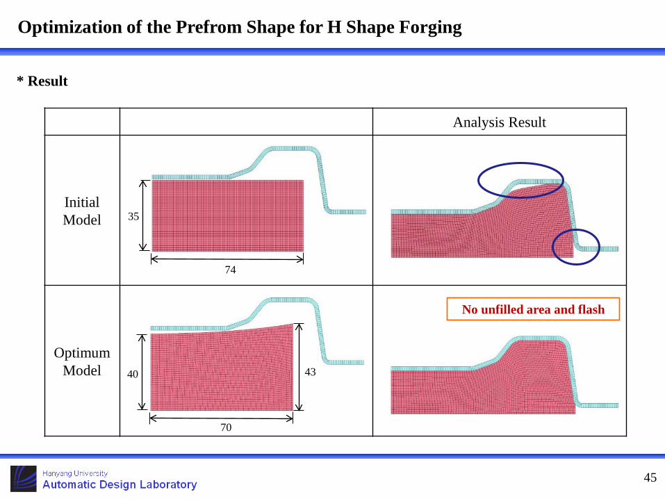
Optimization of the Prefrom Shape for H Shape Forging
45
* Result
No unfilled area and flash
74
35
70
40 43
Analysis Result
Initial Model
Optimum Model
Optimization of the Prefrom Shape for H Shape Forging

46
ESLSO Software

47
Software Development
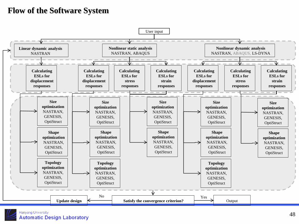
• Software is developed using C and C++ on the Windows system.
• ESLSO software system has been developed based on the theory of ESLSO.
• Linear dynamic, nonlinear static and nonlinear dynamic response optimization using ESLs are supported in the software system.
• Ls-DYNA and Nastran can be utilized for finite element analysis while linear static response optimization using Nastran, Genesis and OptiStruct.
• ESLs for displacement, stress and/or strain constraints are included in the current software system.
48
Flow of the Software System
User input
Linear dynamic analysis NASTRAN
Nonlinear dynamic analysis NASTRAN, ABAQUS, LS-DYNA
Calculating ESLs for
displacement responses
Calculating ESLs for
displacement responses
Calculating ESLs for
stress responses
Calculating ESLs for
strain responses
Calculating ESLs for
displacement responses
Calculating ESLs for
stress responses
Calculating ESLs for
strain responses
Size optimization NASTRAN, GENESIS, OptiStruct
Shape optimization NASTRAN, GENESIS, OptiStruct
Topology optimization NASTRAN, GENESIS, OptiStruct
Satisfy the convergence criterion?
Size optimization NASTRAN, GENESIS, OptiStruct
Shape optimization NASTRAN, GENESIS, OptiStruct
Topology optimization NASTRAN, GENESIS, OptiStruct
Size optimization NASTRAN, GENESIS, OptiStruct
Shape optimization NASTRAN, GENESIS, OptiStruct
Size optimization NASTRAN, GENESIS, OptiStruct
Shape optimization NASTRAN, GENESIS, OptiStruct
Topology optimization NASTRAN, GENESIS, OptiStruct
Size optimization NASTRAN, GENESIS, OptiStruct
Shape optimization NASTRAN, GENESIS, OptiStruct
Yes Update design
No Output
Nonlinear static analysis NASTRAN, ABAQUS

49
Current development of ESLSO
a
b
c
Automobile Crash Optimization
50
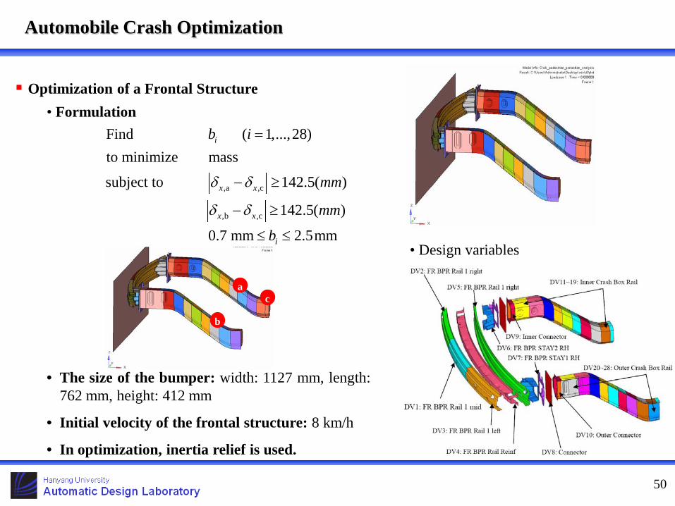
Optimization of a Frontal Structure • Formulation
• Design variables
• The size of the bumper: width: 1127 mm, length: 762 mm, height: 412 mm
• Initial velocity of the frontal structure: 8 km/h
• In optimization, inertia relief is used.
,a ,c
,b ,c
Find ( 1,...,28)to minimize mass
subject to 142.5( )
142.5( )
0.7 mm 2.5mm
i
x x
x x
i
b i
mm
mm
b
δ δ
δ δ
=
− ≥
− ≥
≤ ≤
Automobile Crash Optimization
51
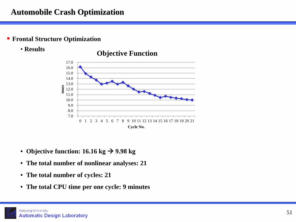
Frontal Structure Optimization • Results
• Objective function: 16.16 kg 9.98 kg
• The total number of nonlinear analyses: 21
• The total number of cycles: 21
• The total CPU time per one cycle: 9 minutes
7.08.09.0
10.011.012.013.014.015.016.017.0
0 1 2 3 4 5 6 7 8 9 10 11 12 13 14 15 16 17 18 19 20 21
mas
s
Cycle No.
Objective Function

Automobile Crash Optimization
52
Side Impact Optimization 1. Initial velocity of the barrier : 50 km/h 2. Rating (Good): The distance between B-pillar point of maximum intrusion and the center line of the seat > 125mm
Automobile Crash Optimization
53
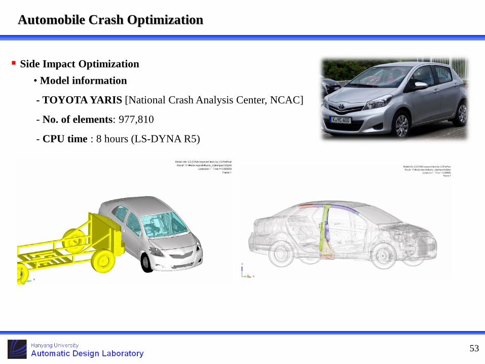
Side Impact Optimization • Model information
- TOYOTA YARIS [National Crash Analysis Center, NCAC]
- No. of elements: 977,810
- CPU time : 8 hours (LS-DYNA R5)
Automobile Crash Optimization
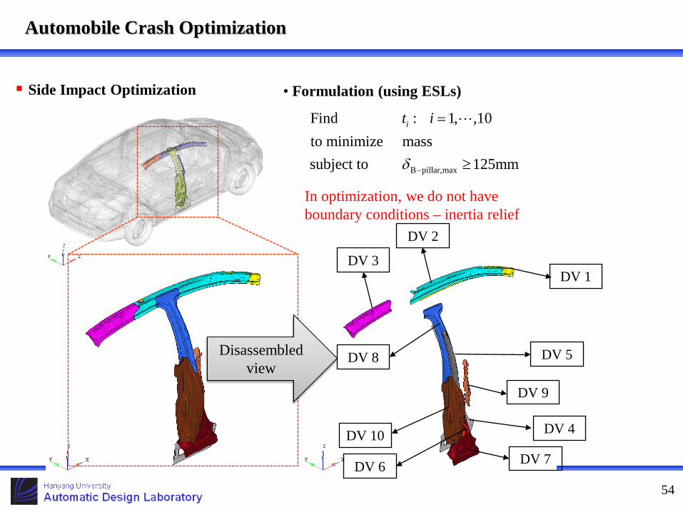
54
Side Impact Optimization
B pillar,max
Find : 1, ,10to minimize masssubject to 125mm
it i
δ −
=
≥
• Formulation (using ESLs)
DV 2
DV 1 DV 3
DV 9
DV 4 DV 10
DV 6 DV 7
DV 8 DV 5
In optimization, we do not have boundary conditions – inertia relief
Disassembled view
Automobile Crash Optimization
55
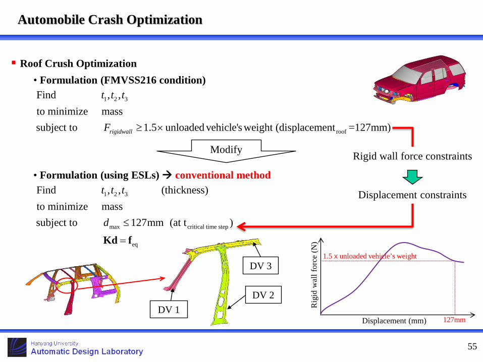
Roof Crush Optimization • Formulation (FMVSS216 condition)
1 2 3
roof
Find , ,to minimize masssubject to 1.5 unloaded vehicle's weight (displacement =127mm)rigidwall
t t t
F ≥ ×
Modify
• Formulation (using ESLs) conventional method 1 2 3
max critical time step
eq
Find , , (thickness)to minimize masssubject to 127mm (at t )
t t t
d ≤
=Kd f
DV 1
DV 3
DV 2
Displacement (mm) R
igid
wal
l for
ce (N
) 127mm
1.5xunloaded vehicle’s weight
Rigid wall force constraints
Displacement constraints

Automobile Crash Optimization
56
Roof Crush Optimization • Formulation (using ESLs) current method
1 2 3 1 2 3
max critical time steps
eq,
eq,
Find , , , , , (thickness,force)to minimize masssubject to 127mm (at t )
f 1.5 unloaded vehicle's weight
f ( node on the contact surface)j
j
t t t p p p
d
j
≤
≥ ×
=∑
Displacement (mm)
Rig
id w
all f
orce
(N)
127mm
1.5xunloaded vehicle’s weight 1p
2p
3p
virtual beams (ESLs)
eq, 1 1
eq 2 2
eq,
ff
f
j i
j i
jn n i
c pc p
c p
= = =
feq,j is proportional to the size of pi.
ESLs
e
e
cn
p
∆p
e: unit direction vector
= feq, j
DV grid (perturbation vector)
eq,f 1.5 unloaded vehicle's weightj ≥ ×∑
cn: distributed force

57
Design optimization of the substructure (Superelement) method
Finite element model
Substructure Method Problems
< Design area: residual >
< Non-design area: superelement > < Finite element model >
• Nonlinear dynamic response optimization
• Generation of substructures: LS-DYNA, MSC.Nastran
• Nonlinear dynamic analysis: LS-DYNA, MSC.Nastran
• Linear static response optimization: MSC.Nastran

58
Optimization process of the substructure method
Formulation
( )( ) ( ) ( )( )
( )N N N N N
N
N
L U
Find to minimize
subject to , , ,
, 0 ( , ) 0; 1, , ( , ) 0; 1, ,
n
i
j
Rf
t t t
th i pg j q
∈
+ +
− =
= =≤ =
≤ ≤
bb
Mz b Cz b K z b z
F bb zb z
b b b
Substructure Method Problems
Divide the structure into a design area and a non-design area
Generate the substructures for the non-design area
Nonlinear dynamic analysis using the substructure and the residual part
Calculate the equivalent static loads for the residual part
Linear static response optimization for the residual part
Converge ?
Yes. No.
Updated design
variables
END

< Design area >
< Non-design area >
59
Substructure Method Problems
If there is no boundary condition in the design area, the inertia relief can be utilized.
< Finite element model >
Formulation
Node 2021
Node 7278
Find 𝑏𝑖 ( i = 1,2,…,10)
to minimize Weight [kg]
subject to 70 ≤ 𝛿𝑥,𝑁𝑁𝑁𝑁#7278 − 𝛿𝑥,𝑁𝑁𝑁𝑁#2021 ≤ 80 [mm]
1.2 ≤ 𝑏𝑖 ≤ 3.5 [mm] (i=1~6)
1.6 ≤ 𝑏𝑖 ≤ 3.5 [mm] (i=7~10)
< Deformed> < Initial >

Simultaneous Optimization of Control and Structural Systems
60
Formulation Since the conventional equivalent static loads method cannot handle the control forces, a new
method is developed.
st
st
st 0
st
LB UBst, st, st,
Find , ( )tominimize ( , ( ), ( ))subject to ( , ( ), ( )) ( )
0 ( 1,2, , )( , ( ), ( ))
0 ( , 1, , )
( 1,2, , )
n
F
j
q q q
R tf t t
t t t t tj m
g t tj m m m
b b b q n
∈
= < <′= =
′ ′≤ = +≤ ≤ =
b ub u z
z h b u z
b u z
0
0 st 0 st( , ( ), ) ( , ( ), ( ), )dft
f ft
f G t t F t t t t= + ∫b z b u z
st st v A 0 1( ) ( ) ( ( ) ) ( ) ( ) ( ) ( ) ( , , , )lt t t t t t t t t+ + + = + =M b z C b H z K z f u
A
ph
vh
xy
z
)(tf
( )u t
B
A st p( ( ) )= +K K b H

Simultaneous Optimization of Control and Structural Systems
61
Equivalent Static Loads Method Analysis domain Design domain
+ = eqf
Equivalent static loads
New design variables The external loads are the functions of
design variables.
st st v A
0 1
( ) ( ) ( ( ) ) ( ) ( ) ( ) ( )( , , , )l
t t t t tt t t t
+ + + = +
=
M b z C b H z K z f u
T Tst v p
Tst v p 1 2
A eq1 eq2 eq3
v p
LB UB
Find where [ , , , ]
to minimize ( , , , , , , ) where [ , , , ]
subject to ( ) ( ) ( ) ( 0,1, , )
( , , , , , , ) 0 ( 1,2, , )
( 1, 2, , )
n
l
w
q q q
R h h
f h h u u us s s s l
g h h w m
q n
∈ =
=
= + + =
≤ =
≤ ≤ =
b b b u
b u z z z uK z f f f
b u z z z
b b b
{ } [ ] [ ]
eq A
st st v
eq1 eq2 eq3
( ) ( )
( ) ( ) ( ) ( ) ( ) ( ) ( )
( ) ( ) ( )
s t
t t t t t
s s s
=
= − + + − + = + +
f K z
f M b z C b z H z u
f f f
xy
z
A
{ }st st( ) ( ) ( ) ( ) ( )t t t− −f M b z C b z
eq1fB
v ( )t−H z
A eq2fB +
( )tu
A eq3fB

Simultaneous Optimization of Control and Structural Systems
62
An external load can be expressed by a shape variable of a virtual beam and a distributed force. It is the same as the hydroforming case.
Design domain
T Tst v p
Tst v p 1 2
A eq1 eq2 eq3
v p
LB UB
Find where [ , , , ]
tominimize ( , , , , , , ) where [ , , , ]
subject to ( ) ( ) ( ) ( 0,1, , )
( , , , , , , ) 0 ( 1,2, , )
( 1,2, , )
n
l
w
q q q
R h h
f h h u u us s s s l
g h h w m
q n
∈ =
=
= + + =
≤ =
≤ ≤ =
b b b u
b u z z z uK z f f f
b u z z z
b b b
B
( )sud
d
A
( )ccz ⋅)(A s
vhc
t, s 43210 sssss
u1 u2
u3 u4
u0
( )u t
Simultaneous Optimization of Control and Structural Systems
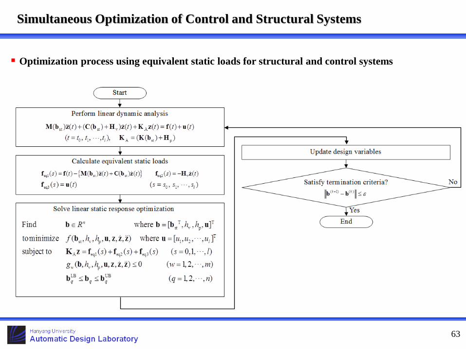
63
Optimization process using equivalent static loads for structural and control systems
No

Simultaneous Optimization of Control and Structural Systems
64
Example: Single degree of freedom linear impact absorber
{ }p v
12.0 2 2 2
0.0
p
v
Find , , ( 1,2, ,100)
tominimize 100.0 1.0 0.005
subject to 0.6mm 0.6mm0.100kN/mm 1.000kN/mm
0.300kN ms/mm 1.194kN ms/mm0 2.000kN
i
i
h h u i
J x x u dt
xh
hu
=
= + +
− ≤ ≤≤ ≤
⋅ ≤ ≤ ⋅
≤ ≤
∫
M
Initial
velocity
u
x
0%
5%
10%
15%
20%
25%
30%
35%
40%
75
85
95
105
115
125
135
0 1 2 3 4 5 6
Con
stra
int v
iola
tion
Obj
ectiv
e fu
nctio
n
Cycle (#)
Objective function & constraint violationObjective function Constraint violation
-0.4
-0.2
0.0
0.2
0.4
0.6
0.8
1.0
0 3 6 9 12Dis
plac
emen
t (m
m)
Time (ms)
Displacementinitial (#0) optimum (#6)
-0.4
-0.2
0
0.2
0.4
0.6
0.8
0 3 6 9 12
forc
e (k
N)
Time (ms)
Actuator force, u(t)initial (#0) optimum (#6)
hp
hv
Results: hp 0.597→1.000kN/mm, hv 0.597→0.686kN·ms/mm, objective function 82.9→115.3
Simultaneous Optimization of Control and Structural Systems
65
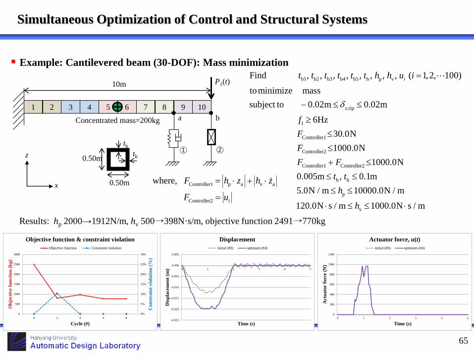
Example: Cantilevered beam (30-DOF): Mass minimization b1 b2 b3 b4 b5 h p v
z,tip
1
Controller1
Controller2
Controller1 Controller2
b h
p
Find , , , , , , , , ( 1,2, 100)
tominimize masssubject to 0.02m 0.02m
6Hz30.0N1000.0N
1000.0N0.005m , 0.1m5.0N / m 10000.0
it t t t t t h h u i
fFFF F
t th
δ
=
− ≤ ≤
≥≤
≤
+ ≤
≤ ≤
≤ ≤
v
N / m
120.0N s / m 1000.0N s / mh⋅ ≤ ≤ ⋅
Controller1 p a v a
Controller2
where,
i
F h z h z
F u
= ⋅ + ⋅
=
1 2 3 4 5 6 7 8 9 10
a b
① ②
10m
Concentrated mass=200kg
P1(t)
0.50m
0.50m
th
tb
0%
5%
10%
15%
20%
25%
30%
0
500
1000
1500
2000
2500
3000
0 1 2 3 4
Con
stra
int v
iola
tion
(%)
Obj
ectiv
e fu
nctio
n (k
g)
Cycle (#)
Objective function & constraint violationObjective function Constraint violation
-0.025
-0.020
-0.015
-0.010
-0.005
0.000
0.005
0 1 2 3 4 5
Dis
plac
emen
t (m
)
Time (s)
Displacementinitial (#0) optimum (#4)
0
200
400
600
800
1000
1200
0 1 2 3 4 5
Act
uato
r fo
rce
(N)
Time (s)
Actuator force, u(t)initial (#0) optimum (#4)
Results: hp 2000→1912N/m, hv 500→398N·s/m, objective function 2491→770kg
x
z

Simultaneous Optimization of Control and Structural Systems
66
Example: Cantilevered beam (30-DOF): Control energy minimization
1 2 3 4 5 6 7 8 9 10
a b
① ②
10m
Concentrated mass=200kg
P1(t)
0.50m
0.50m
th
tb
Results: hp 2000→998N/m, hv 500→591N·s/m, objective function 2644→1322N·s
b1 b2 b3 b4 b5 h p v
tip
1
b h
p
v
Find , , , , , , , , ( 1,2, 100)
tominimize control energy (N s)subject to 0.03m 0.03m
6Hzmass 650kg0.005m , 0.1m5.0N / m 10000.0N / m
120.0N s / m 1000.0N s / m
it t t t t t h h u i
f
t th
h
δ
=
⋅− ≤ ≤
≥≤≤ ≤
≤ ≤
⋅ ≤ ≤ ⋅
{ }5
p a v a0controlenergy ( ) ( ) ( )h z t h z t u t dt= ⋅ + ⋅ +∫
x
z
0%
10%
20%
30%
40%
50%
60%
0
500
1000
1500
2000
2500
3000
0 1 2 3
Con
stra
int v
iola
tion
(%)
Obj
ectiv
e fu
nctio
n (N
·s)
Cycle (#)
Objective function & constraint violationObjective function Constraint violation
-0.050
-0.040
-0.030
-0.020
-0.010
0.000
0.010
0 1 2 3 4 5
Dis
plac
emen
t (m
)
Time (s)
Displacementinitial (#0) optimum (#3)
-500
0
500
1000
1500
2000
2500
0 1 2 3 4 5
Act
uato
r fo
rce
(N)
Time (s)
Actuator force, u(t)initial (#0) optimum (#3)
Earthquake Problems
67
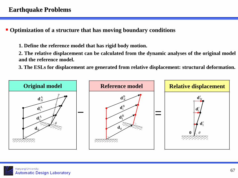
Optimization of a structure that has moving boundary conditions
1. Define the reference model that has rigid body motion. 2. The relative displacement can be calculated from the dynamic analyses of the original model
and the reference model. 3. The ESLs for displacement are generated from relative displacement: structural deformation.
Reference model
ANd
Aid
A1d
0d
BNd
Bid
B1d
0d
Original model Relative displacement
0
r1d
rid
rNd
− =θ
θ
68
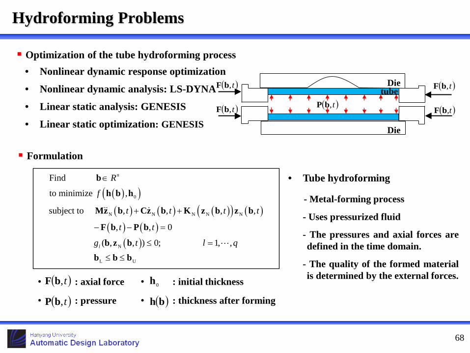
Optimization of the tube hydroforming process • Nonlinear dynamic response optimization
• Nonlinear dynamic analysis: LS-DYNA
• Linear static analysis: GENESIS
• Linear static optimization: GENESIS
Formulation
( )t,bF
( )t,bP
Die
Die
tube
( )t,bF
( )t,bF
( ),tbF
( )( )( ) ( ) ( )( ) ( )
( ) ( )( )
0
N N N N N
N
L U
Find
to minimize ,
subject to , , , ,
, , 0
( , , ) 0; 1, ,
n
l
R
f
t t t t
t t
g t l q
∈
+ +
− − =
≤ =
≤ ≤
b
h b h
Mz b Cz b K z b z b
F b P b
b z bb b b
• : axial force
• : pressure
• : initial thickness
• : thickness after forming
( )t,bF
( )t,bP
0h
( )bh
• Tube hydroforming
- Metal-forming process
- Uses pressurized fluid
- The pressures and axial forces are defined in the time domain.
- The quality of the formed material is determined by the external forces.
Hydroforming Problems
69
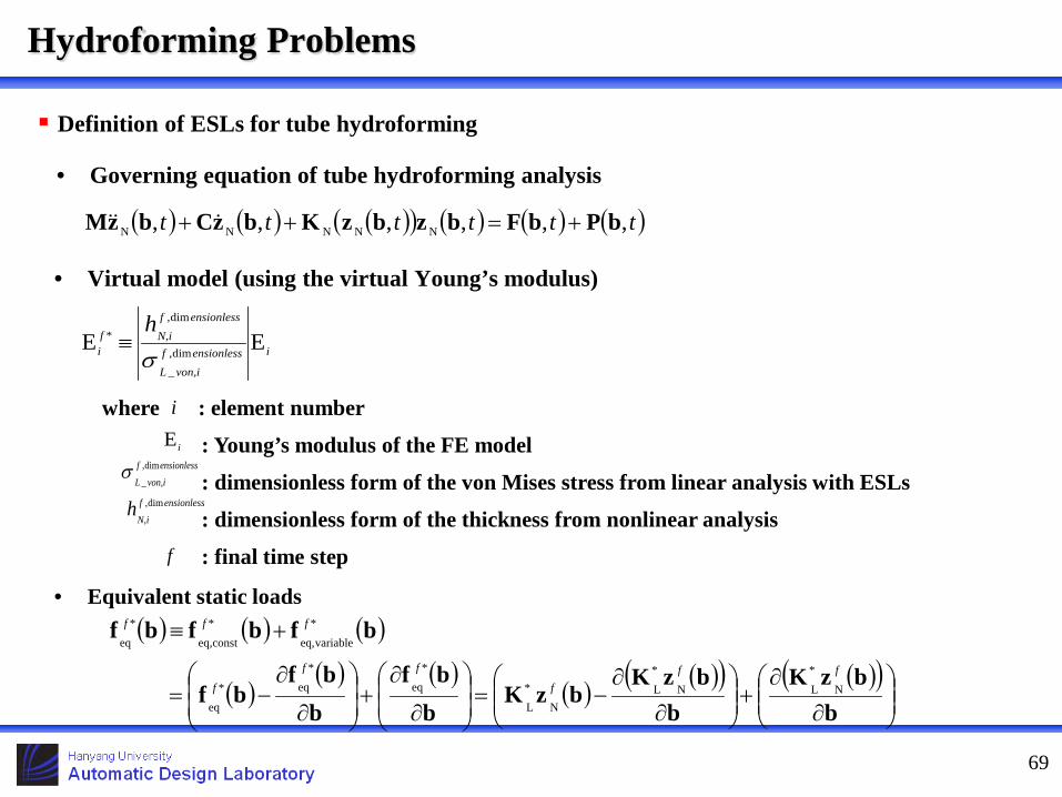
Definition of ESLs for tube hydroforming
• Governing equation of tube hydroforming analysis
• Equivalent static loads
( ) ( ) ( )( ) ( ) ( ) ( )tttttt ,,,,,, NNNNN bPbFbzbzKbzCbzM +=++
• Virtual model (using the virtual Young’s modulus)
iensionlessfvon,iL
ensionlessfN,if
i
hEE dim,
_
dim,*
σ≡
where : element number
: Young’s modulus of the FE model
: dimensionless form of the von Mises stress from linear analysis with ESLs
: dimensionless form of the thickness from nonlinear analysis
: final time step
i
iEensionlessf
von,iLdim,
_σ
ensionlessfN,i
h dim,
f
( ) ( ) ( )
( )( ) ( )
( ) ( )( ) ( )( )
∂
∂+
∂
∂−=
∂
∂+
∂
∂−=
+≡
bbzK
bbzK
bzKb
bfb
bfbf
bfbfbfff
f
ff
f
fff
N
*
LN
*
LN
*
L
*
eq
*
eq*
eq
*
variableeq,
*
consteq,
*
eq
Hydroforming Problems
70
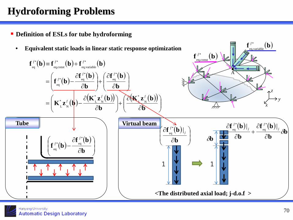
Definition of ESLs for tube hydroforming
• Equivalent static loads in linear static response optimization
( ) ( ) ( )
( )( ) ( )
( ) ( )( ) ( )( )
∂
∂+
∂
∂−=
∂
∂+
∂
∂−=
+≡
bbzK
bbzK
bzK
bbf
bbf
bf
bfbfbf
f*f*f*
*f*f
*f
*f*f*f
NLNLNL
eqeq
eq
variableeq,consteq,eq
<The distributed axial load; j-d.o.f >
1 1
( )( )
∂
∂−
bbf
bf*
eq*
eq
f
f
( )
∂
∂
bbf j
f |*
eq
( ) ( )b
bbf
bbf
δ∂
∂+
∂
∂ jf
jf || *
eq
*
eq
bδ
Tube Virtual beam
xy
z
A
( )bf *fvariableeq,
( )bf *fconsteq,
Hydroforming Problems

71
Definition of ESLs for tube hydroforming
• Linear static response optimization
- Formulation: The external forces are functions of design variables.
- The points of the profiles are design variables.
- Basis functions can be used for the expression of the axial forces and pressures.
- and are design variables.
- The number of design variables can be reduced.
( )( )( ) ( )( )( )
UL
L
eqLL
0
1 0
0 subject to minimize to Find
bbbbzb
bfbzKhbh
b
≤≤
=≤
=−
∈
q,,l;,g
,fR
*fl
*f*f*
n
( ) ( )( ) ( )∑=
∑=
=
=
npk di
nfk di
uBu
uBu
1 ,i
1 ,i
PP
FF ( )otherwise
if 01 1
1+<≤
= ii,i
uuu,,
uB
( ) ( ) ( )uBuuuuuB
uuuuuB d,i
idi
did,i
idi
id,i 11
11
1−+
++
+−
−+ −−
+−
−=
ia ic
<Force profile> t
1t 2t 3t
( )tF
ft1−ft1b2b
3b
1−fb fb
<Pressure profile> t
1t 2t 3t
( ) tP
ft1−ft
1+fb 2+fb 3+fb
12 −fb fb2
=i
i
at
iF
=i
i
ct
iP
Hydroforming Problems


![[PPT]Slide 1 - UFL · Web viewWhen does nonlinear analysis experience difficulty? Nonlinear Structural Problems What is a nonlinear structural problem? Everything except for linear](https://cdn.vdocuments.us/doc/165x107/5abe84a67f8b9a8e3f8d1825/pptslide-1-ufl-viewwhen-does-nonlinear-analysis-experience-difficulty-nonlinear.jpg)


