1
Quasi-Experiments and Hedonic Property ValueMethods ∗
Christopher F. Parmeter† and Jaren C. Pope‡
September 2, 2012
∗The authors would like to thank Nick Kuminoff and V. Kerry Smith for providing excellent commentsthat lead to a more cohesive version of this chapter. All errors belong to us.†Christopher F. Parmeter, Department of Economics, University of Miami, Coral Gables, FL 33124. Phone:
305-284-4397, Fax: 305-284-, E-mail: [email protected].‡Jaren C. Pope, Department of Economics, Brigham Young University, Provo, UT 84602. Phone: 801-422-
2037,E-mail: [email protected].

2
Abstract
There has recently been a dramatic increase in the number of papers that havecombined quasi-experimental methods with hedonic property models. This is largelydue to the concern that cross-sectional hedonic methods may be severely biased byomitted variables. While the empirical literature has developed extensively, there has notbeen a consistent treatment of the theory and methods of combining hedonic propertymodels with quasi-experiments. The purpose of this chapter is to fill this void. Aneffort is made to provide background information on the traditional hedonic theory,the traditional cross-sectional hedonic methods as well as the newer quasi-experimentalhedonic methods that use program evaluation techniques. By connecting these twoliteratures, the underlying theoretical and empirical assumptions necessary to estimatethe marginal willingness to pay for a housing characteristic are highlighted. The chapteralso provides a practical “how to” guide on implementing a quasi-experimental hedonicanalysis. This is done by focusing on a series of steps that can help to ensure thereliability of a quasi-experimental identification strategy. We illustrate this process usingseveral recent papers from the literature.
JEL Classification: C9, D6, Q5, R0.
Keywords: Regression Discontinuity, Differences-in-Differences, Property Value, Pro-gram Evaluation, Marginal Willingness to Pay, Capitalization, Hedonic, Quasi-Experiment.

3
1 Introduction
Households’ valuations of environmental and urban amenities are often imbedded in the prices
of transacted property. Property prices are one of the few market based measures that can be
used to reveal the values of many environmental and urban amenities that are not explicitly
traded in their own markets. Researchers and policymakers are often interested in quantifying
the value of a single amenity such as air quality or school quality. However, extracting the “im-
plicit price” of one amenity from the overall prices in a property market can be a challenging
task. The most commonly used method for estimating an implicit price from property values
is called the “hedonic method”. This method was first used by Haas (1922), Waugh (1928)
and Court (1939), was later popularized by Griliches (1971), and was given a welfare theoretic
interpretation by Rosen (1974). This cross-sectional approach of regressing the attributes of
a differentiated product on product prices has been widely applied to real estate markets to
understand household’s marginal willingness to pay for changes in environmental and urban
attributes.
In recent years, there has been increasing concern that the implicit prices estimated using
the “traditional” hedonic method may often be biased because of omitted variables that
confound a cross-sectional identification strategy. From an experimentalist’s perspective, the
ideal way to identify the value of an amenity, would be to randomly adjust the quantity/quality
of the amenity in different neighborhoods of a housing market, and then record the impact
that the random changes in the amenity of interest have on housing prices. In a laboratory
setting the investigator has control of the housing attributes, budget sets, and the ‘location’
of houses. This provides the investigator with ceteris paribus outcomes of individual housing
sales that are difficult to procure in real world settings. However, Levitt and List (2007) have
recently noted that laboratory experiments may not be as ‘generalizable’ to the real world as
previously thought. The natural environments in which people make choices matter.
4
Levitt and List (2007) discuss the benefits of “field experiments” to overcome some of
the limitations of laboratory experiments. A field experiment is an experiment where the
researcher controls randomization, yet participants in the experiment are making choices in
a naturally occurring environment. While their discussion hinges on experiments attempting
to measure pro-social preferences, their insights are easily applied to other experimental con-
texts as well. Given that designing field experiments for the housing market would provide
unique insights covering many different aspects of how home-buyers value urban, spatial, and
environmental amenities, this line of research appears to be warranted. However, currently
there is a dearth of field experiments that pay attention to “big ticket” items, because of the
costs involved. The bulk of currently implemented field experiments focus on social prefer-
ences using low budget items. Nonetheless, a field experiment in the housing market can be
thought of as a type of “gold standard”.
Unfortunately, this experimental “gold standard” is, for obvious reasons, difficult to im-
plement in housing markets because of cost and ethical considerations.1 For this reason,
researchers have begun to explore a myriad of quasi-experiments that have occurred from na-
ture or man-made policies that help to identify a causal impact of the change in an amenity on
housing prices. Recent examples of this genre of hedonic work include: value of school qual-
ity (Black (1999) and Figlio and Lucas (2004)), value of air quality (Chay and Greenstone
(2005)), value of airport noise (Pope (2008a)), value of hazardous waste and toxic releases
(Bui and Mayer (2003) and Gayer, Hamilton and Viscusi (2000)), value of flood risk reduction
(Hallstrom and Smith (2006) and Pope (2008b)), and value of crime reduction (Linden and
Rockoff (2008) and Pope (2008c)).2
This chapter explores the theory and practice of quasi-experiments in housing markets.
1This point relates to a criticism of experimental economics, which has been that many of the resultsgenerated from the lab or even in the field using low-cost goods may not apply to high-cost goods like houses.
2Early work by Brookshire, Tschirhart and Schulze (1985), Kask and Maani (1992), Kiel and McClain(1995), and others were also using a quasi-experimental approach, but did not use the vocabulary popularizedby labor economics and therefore have been somewhat forgotten as pioneers in this genre.
5
Although there have been several excellent book chapters and many reviews on the hedonic
method over the years (see for example Palmquist (2005), Taylor (2003), Freeman (1993) and
Bartik and Smith (1987)), there has not been a review or a comprehensive chapter on the
quasi-experimental approach applied to the hedonic method. We think that this chapter can
fill this gap in the literature and make two broad contributions. Our first contribution is
to describe the economic and econometric theory that relates to quasi-experimental hedonic
methods. We provide background on hedonic theory and its relation to quasi-experiments.
An attempt is made to clarify the underlying theoretical and empirical assumptions that are
needed to move from a cross-sectional hedonic to a hedonic model that uses the temporal
dimension to identify the impact of a quasi-experimental treatment that occurs in time and
space. Furthermore we describe the alternative econometric models that can potentially be
used in conjunction with housing data to estimate the impact of a quasi-experiment on housing
prices.
The second broad contribution of this chapter is to focus on some important steps of a
careful quasi-experimental analysis using the hedonic method which have often been glossed
over in the literature. We outline a series of steps that should be undertaken to better ensure
the reliability of an identification strategy that combines a quasi-experiment with property
data. This involves a focus on data quality, exogeneity of the treatment, the importance of
adequately controlling for spatial and temporal unobservables, and empirical specification.
Finally, we illustrate the importance of these steps using three recent papers that have been
published in some of the top general interest and field journals of economics. It is our hope
that the chapter will clarify some of the interesting theoretical and empirical issues that have
arisen in recent years as researchers have combined quasi-experiments with housing data.
Furthermore, we hope that the chapter will provide a guide to researchers interested in using
this methodology.
The chapter is organized much like a typical hedonic journal article by describing the
6
theory, econometrics, data and then the application. More precisely, section 2 lays out the
traditional hedonic theory developed by Rosen (1974) and others. This section also describes
how the traditional hedonic method has been applied in empirical settings. Section 3 de-
scribes the econometrics of estimating quasi-random experiments in property markets. It also
discusses the assumptions necessary to relate capitalization of an exogenous event with the
welfare measures of the hedonic model following a recent paper by Kuminoff and Pope (2009).
Section 4 describes the general empirical steps necessary to identify the price impact of a
quasi-experiment in the housing market. In section 5, three recent papers that have used the
quasi-experimental hedonic method are described to illustrate the importance of the steps
provided in section 4. Finally, section 6 concludes the chapter.
2 Traditional hedonic methods
In this section we describe the theory of the traditional hedonic model and how it has been
used empirically. An understanding of the theoretical and empirical assumptions underly-
ing the traditional hedonic method helps one to understand the strengths and weaknesses
of the quasi-experimental hedonic method that is described in sections 3-5. The interpre-
tation of coefficients in both traditional and quasi-experimental hedonic analyses rely on a
set of theoretical and empirical judgements/assumptions. Thus, this section outlines the
judgements/assumptions that are made in a traditional hedonic analysis to prepare us for a
discussion of the judgements/assumptions needed in a quasi-experimental hedonic analysis.
2.1 Theory
Houses exhibit substantial heterogeneity. As such, economists have thought of them as being
part of a differentiated product market rather than in a homogeneous product market. In a
differentiated product market, people consider all the varieties of the good before they choose
7
a “type”. Under these conditions, there is a price schedule for these products even when the
market in which they are traded is characterized as competitive. The economic model put
forth by Rosen (1974) provides a description of a competitive equilibrium where buyer and
seller interaction takes place in a differentiated product market such as the housing market.
Rosen’s hedonic model maintains that a house along with the services conveyed by its location
can be characterized by a vector of observable attributes z = 〈z1, z2, . . . , zq〉, where zi measures
the amount of the ith attribute that the house contains. The z’s could measure square footage,
the number of bathrooms, the distance to a park, proximity to a shopping center, the quality
of the air and water for the house, etc. In the hedonic price index literature the z’s can be
thought of as rough measures of quality.
Rosen’s model assumes that buyers and sellers are fully informed. This means that they
are aware of all the prices of houses for sale and the amount of each attribute available to
any given house. Furthermore, it is assumed that the market is competitive and that buyers
and sellers act as price-takers and so can not influence the market price schedule. It is also
assumed that the market contains a “sufficiently large” number of houses ensuring that a
buyer’s choice appears to have been made from a set of houses with continuously varying
amounts of attributes. That is, choice of a house can be represented as if it was a choice of a
bundle of attributes.3
The hedonic price function is in general nonlinear suggesting that the product cannot be
unbundled and the individual attributes sold in separate markets. This implies that arbitrage
possibilities do not exist for consumers or sellers to eliminate price differences across the
product. This also follows from the full information assumption about prices. With full
information, consumers know of all prices for an identical good and can purchase from the
seller with the lowest price. Knowledge of all existing prices disallows arbitrage opportunities
3Here bundle refers to the vector of attributes that the consumer is purchasing when the house is beingconsumed; it is used interchangeably with attribute vector. Lancaster (1966) analyzed the consumer side ofthe market without assuming continuity of attribute bundles.
8
in equilibrium.
Rosen’s model provides the theoretical underpinnings for the hedonic price model, assum-
ing perfectly competitive markets and full information within the market. Indeed, his model
was the first to theoretically show that the hedonic price function was simultaneously an en-
velope for buyers’ bid functions and sellers’ offer functions. To clarify Rosen’s insight we look
more closely at the hedonic model on both the consumer and producer sides of the market.
2.1.1 The consumer side of the market
Consider a competitive housing market. Let P (z) represent the hedonic price function from
which consumers base their decisions, where z is again the vector of housing attributes. A
representative consumer has utility function U(x, z, ζ), where x represents a composite com-
modity reflecting consumption of all other goods and ζ is a vector of taste parameters that
characterize the utility function and have joint distribution f(ζ).4 The composite commodity
is assumed to have unit price. Rosen follows the traditional beliefs of the utility function,
strict concavity and monotonicity in each attribute. The consumer’s budget constraint is
given as y = x + P (z) where y represents income. If P (z) was linear this would be the
standard constrained utility maximization problem, however, given that P (z) is nonlinear the
analysis leads to a somewhat different picture of market equilibrium. Replacing composite
consumption within the utility function as x = y − P (z) the first order conditions are,
Uz(y − P (z), z, ζ)− Ux(y − P (z), z, ζ) · Pz(z) = 0. (1)
Rearranging (1) shows the fundamental trait of the hedonic price function: the slope of
the hedonic price function (in the ith attribute) represents the marginal rate of substitution
between this attribute and the composite commodity, holding all other attributes fixed (Pz =
4In an econometric setting ζ would be composed of those parameters that are observed, ζo, and thoseparameters that are unobserved (by the econometrician), ζuo.

9
Uz/Ux). It should be noted that only in the special case when the marginal utility of the
composite commodity is constant does the slope of the hedonic price function represent a
classic compensated demand curve.5
Rosen described a buyer’s maximum “bid” for a house with a bid function, θ(z;u, y) that
holds utility and income fixed. It represents the expenditure a consumer is willing to pay for
different attribute vectors for a given utility-income index. Thus, it traces out a family of
indifference curves relating the attributes with forgone amounts of the composite commodity.
Incorporating the bid function into the utility function in the same manner as the hedonic
price function, U(y − θ, z, ζ) = u, results in the following first order conditions,
Uz(y − θ, z, ζ)− Ux(y − θ, z, ζ) · θz(z) = 0, (2)
which looks almost identical to (1).
Given that both the bid function and the hedonic price function satisfy the same condition,
it is evident that in equilibrium consumer’s bid functions are tangent to the market hedonic
price function. This in turn suggests that the hedonic price function represents an envelope
of consumer’s bid functions in equilibrium. For u1 > u2 it is the case that θ(z; y, u1) lies
everywhere beneath θ(z; y, u2). That this is so follows from the fact that with the same income
and attribute vector, to achieve a higher utility level the bid must be lower, so as to have more
money left over for other consumption. Thus, the hedonic price function represents an upper
envelope and equilibrium is characterized by the hedonic price function being everywhere
above the family of bid functions that correspond to this equilibrium. An illustration of
equilibrium for one dimension of z is presented in Figure 2.1 for three different consumers.
Figure 2.1 about here, Caption: Buyer equilibrium.
5This fact was largely ignored in the subsequent years following Rosen’s paper and many of the papersthat employed his methodology econometrically misinterpreted their results, basing their estimates on demandfunctions rather than marginal rate of substitution functions.
10
It is apparent from Figure 2.1 that the hedonic price function is more steeply curved to the
right of a tangency (and less steeply curved to the left of a tangency) than the bid functions.
If this were not the case then the first order conditions for utility maximization would not be
satisfied as the tangency points would break down. The curvature conditions suggest that the
consumer does not want to move from the current point because the movement would result
in an overpayment and a net loss. Another insight that can be gathered from the figure is that
consumers with similar tastes and incomes will locate around similar product specifications.
Thus, the hedonic price method can explain market segmentation and corresponds nicely with
spatial models of equilibrium.
2.1.2 The producer side of the market
Rosen also analyzed optimality conditions for sellers using a standard profit maximizing frame-
work. Here house sellers produced M units of housing and took prices as given. Costs for the
house seller were characterized by the industry cost function, C(M, z, υ), where υ represents
cost (production) parameters that vary across sellers with joint distribution f(υ). As with
consumer taste parameters, υ is composed of parameters that are observed, υo and parame-
ters that are unobserved by the econometrician, υuo. Again, Rosen made typical assumptions
regarding the cost function, namely convexity and positive marginal costs for both attributes
and number of units. Thus, in Rosen’s profit maximizing framework with the hedonic price
function given, the first order conditions satisfied by sellers were,
M · Pz(z) =Cz(M, z, υ) (3)
P (z) =CM(M, z, υ). (4)
The first order conditions, at the optimum values of the characteristics, suggest that the
slope of the hedonic price function (marginal revenue) equal the marginal cost of production,

11
equation (3), and the marginal cost of selling another unit equals the hedonic price (unit
revenue), equation (4).
The symmetry with the consumer side of the analysis becomes apparent with the definition
of an offer curve. The offer curve, ψ(z; π), is the seller’s version of a consumer’s bid function.
Here sellers offer different levels of the attribute vector for a fixed profit. These curves trace
out iso-profit relationships between the individual attributes. Here, as with the consumer
analysis, the hedonic price function is replaced by sellers’ offer functions and the subsequent
first order conditions derived. Not surprisingly they look almost identical to (3) through (4).
M · ψz =Cz(M, z, η) (5)
ψπ =1/M (6)
As before, the first order conditions imply that the marginal offer price (at constant profit) is
equal to the marginal cost of production while the marginal offer price (at constant attribute
levels) is constant, thus, offer functions for different levels of profit with the same attribute
vectors have the same slope. For higher levels of profit (π1 > π2) a seller’s offer function
should be higher than for a lower profit level, ψ(z; π1) > ψ(z; π2). Intuitively this means that
for the same attribute vector (and cost of production), to obtain a higher level of profit, the
seller must offer the house for a higher price. Thus, for any given seller, the offer functions
lie strictly above one another and the first order condition implies that the hedonic price
function represents a lower envelope of these offer functions with equilibrium corresponding
to the hedonic price function being everywhere beneath and tangent to the profit-attribute
indifference surface.
An example for one dimension of z is provided in Figure 2.2. Here, as opposed to the
consumer side, the hedonic price function is less curved than sellers’ offer functions. If the
curvature were less than sellers’ offer functions then sellers would not be producing at optimal
12
levels and would need to adjust. Even though the results for consumers suggests separation
based on specific attributes, here segmentation of sellers is not quite as obvious. One interpre-
tation may be that certain types of sellers sell certain packages of the goods. However, most
hedonic analyses in the context of the housing market have assumed that the supply of homes
is fixed, at least in the short-run, with the market composed primarily of the existing stock.
“Sellers” in the short-run are simply owners of the existing housing stock who have decided
to put their house up for sale. Sellers attempt to utility maximize, which in this case results
from maximizing profits, just like buyers. In a competitive market, sellers viewed from this
perspective are simply price takers just as buyers.
Figure 2.2 about here, Caption: Seller equilibrium.
2.1.3 Hedonic equilibrium
In equilibrium the matching of buyers and sellers forms a locus of equilibrium transaction
prices where the familes of bid and offer curves are tangent. In a world of heterogeneity in
preferences, income and production costs, the equilibrium price locus represents the upper
envelopes of buyer’s bids and the lower envelopes of seller’s offers. A graphical representation
of equilibrium is given in Figure 2.3. We see that, in equilibrium, buyers’ bid functions are
less curved than the hedonic price function, which in turn is less curved than sellers’ offer
functions. In fact, it can be shown that the hedonic price function is a weighted average of
buyers’ bid functions and sellers’ offer functions.
Figure 2.3 about here, Caption: Hedonic market equilibrium.
Under the assumption of an interior solution where consumers buy only one house and
the price of all other goods (x) is normalized to 1, the Rosen framework we have described
suggests that,
∂P (z)
∂z=∂θ(z)
∂z=∂ψ(z)
∂z. (7)

13
This equation implies that the marginal price reveals the marginal willingness to pay (MWTP)
or the marginal rate of substitution between the attribute and the composite good, x, for
buyers. Estimation of these implicit marginal prices has been the focus of the majority of
empirical hedonic analyses and is referred to as the “first stage” of the hedonic.6
2.2 Traditional hedonic empirical methods
Now we turn to the empirical implementation of the traditional hedonic method. In order to
identify a MWTP in a first stage hedonic, the theoretical assumptions from the hedonic model
must be satisfied as well as a set of empirical assumptions/judgements. Of course to begin, a
researcher would gather data on the housing market of interest and regress house sale prices
on the structural, urban, and environmental characteristics present in the house. That is, for
a house that sells at price Pi with characteristics Xi, the regression of interest is
Pi = m(Xi; β) + εi, (8)
for the n houses in the dataset. We note that in the remainder of this chapter regression co-
variates will commonly be denoted with X. In the discussion of the traditional hedonic theory
housing attributes were symbolized with z, however, throughout the empirical portions of this
paper we use the standard textbook notation for covariates (Xi). Here the equilibrium hedonic
function m(x; β) can be specified to be linear, m(x; β) = xβ or it can be nonlinear or fully
nonparametric. In the linear setting, the one most commonly used in the quasi-experimental
literature, interest lies in the βs associated with the urban and environmental amenities asso-
ciated with the housing locations. The β’s are the estimates of the slope of the price function
with respect to a particular characteristic Xi. Thus, estimates of these slope coefficients rep-
6Attempts to employ the full two-stage hedonic method are limited. Bartik (1987), Epple (1987) andEkeland, Heckman and Nesheim (2004) discuss ways of overcoming identification problems, but the so called“second stage” of the hedonic model remains difficult to implement in practice.
14
resent MWTP that result from the hedonic equilibrium described earlier in section 2. There is
nothing fancy econometrically about estimating hedonic price functions in general. However,
the interpretation of the the estimated coefficients requires care. For example, in a linear
setup, while the βs may be interpreted as MWTP, in a nonlinear setting this could be entirely
false. Thus, a careful assessment of the underlying econometric assumptions linked to the
theoretical hedonic model is required. Four important issues we consider are: (i) the single
market assumption, (ii) stability of the price function over time, (iii) omitted variable bias,
and (iv) functional form issues.
2.2.1 The single market assumption
The hedonic model (applied to housing) is based on a single housing market. Thus a judge-
ment must be made as to the spatial extent of a housing market. Palmquist (2005) notes that:
“One can say that the units are traded in a single market without implying that everyconsumer is a potential customer for every unit sold in the market. A given consumer mayonly be interested in a segment of the market. However, all that is required for the market tobe integrated is that segments for different consumers overlap.”
Nonetheless this is a very general description for a market. In practice there is going to
be a bias-variance tradeoff in defining a housing market. Is it a neighborhood or the entire
nation? We will discuss this issue more in section 4. See also the expository of Palmquist
(1991) on how best to think about a housing market.7
7Our description of the housing market has not discussed issues surrounding the labor market. Certainlythe labor market is linked to the housing market since many locational decisions are made due to employmentopportunities. Roback (1982) discusses in greater detail the impact that accounting for labor market decisionshas on the classic hedonic model of Rosen and develops a general equilibrium model that accounts for the factthat not all consumers can occupy the same space even if they are identical.

15
2.2.2 Stability over time
Rosen’s hedonic model was considered at a point in time so that preferences were stable and
one could ignore shocks to the market that may have introduced a disequilibrium. When
one extends this analysis to allow for house sales at different points in time then an im-
plicit assumption of either identical preferences over time or proper conditioning on changing
preferences needs to be made.
What is key to recognize here is that if one were solely interested in estimating a hedonic
function in a cross section setting then time stability is irrelevant. However, quasi-experiments
usually require a temporal element for the analysis to provide meaningful results. They take a
before-after approach and the time gap associated with the before-after has significant impacts
on the reliability of the estimates of a given policy. To make claims about the impact of a
policy ones needs to minimize the temporal window around which a policy change occurs.
Again, there are two constraints on this temporal window. First, enough transactions have
to occur both before and after for the experimenter to have enough data to reliably estimate
a policy impact. Second, the window has to be narrow enough to be confident that nothing
else in the economic landscape has changed that would degrade the policy impact estimate.
Again, this narrowing of the temporal window is akin to a bias-variance tradeoff and it is the
judgment of the researcher to determine the appropriate size of the window. Many criticisms
levied against quasi-experimental hedonic studies have been focused on the time gap associated
with the before-after of the policy. Inevitably, data constraints will provide some impediment
for attaining the appropriate window width around the policy.
2.2.3 Omitted variable bias
The traditional hedonic theory suggests that a house represents a bundle of attributes. How-
ever, it makes no claim as to how many and which attributes those are. This makes adequate

16
statistical estimation difficult because parameter estimates of the attributes in the model
will be biased if there are omitted attributes. One can think of these omitted attributes as
representing an index, ξ = γ1zo1 + · · · γpzop. This index is quite different from the random
component in a standard regression. In most settings the random component represents un-
observed shocks to the system, measurement errors, and random variation in the the data, but
with a hedonic regression, while this random component still exists, the omitted attributes
index is there as well.
One can see from this setup that with omitted attributes, not only does one obtain biased
estimates, but heteroscedasticity, if not already present, surely exists now. As we will discuss
later, the use of panel data and/or repeat sales data will introduce a house or neighborhood
specific effect into the model which helps to eliminate the omitted attribute index. Suppose
one were to observe data on a house at two points in time. Then, given that the observed
characteristics are controlled for, the omitted attributes index should be the same for both
instances that this house is represented in the data, unless any of those omitted attributes
changed over time, or the index coefficients changed, or both. Economic arguments against
these types of assumptions are easier to make than ignoring the presence of the index at all.
If one believes that there is less than full information, less than optimal search8 performed
by perspective buyers, and buyers and sellers are allowed to bargain over the final sale price
(all situations that cannot occur in the traditional hedonic framework) then the error term in
a hedonic regression is even more complicated. What is not clear is where the impact of the
violation of these assumptions occurs. That is, if one violates the full information assumption
or the no transaction cost assumption, is the effect through the shape of the hedonic surface
or does it manifest itself in the error attached with estimating this surface. These are issues
8Less than optimal search means that buyers (or sellers) are not maximizing utility given search costsentering their budget constraint. So, a buyer who does not continue searching even though the gain fromadditional search is positive, is not optimally searching. This may be the case for out of town home buyerswho are moving into the area.

17
that are excluded from the traditional hedonic theory.
2.2.4 Functional form issues
Another obvious, but critical, element of implementing a hedonic analysis empirically is proper
specification of the hedonic price function. That is, if the function is itself misspecified, then
it is highly unlikely that the corresponding slope coefficients will represent MWTP as they
do when the empirical model is correctly specified. Thus, care is required when selecting the
empirical model with which to estimate the hedonic function.
One must also consider the application at hand when specifying a hedonic model. Many
housing economists estimate hedonic price functions with the purpose of forecasting housing
prices. In a quasi-experimental setting, interest lies in the change in the hedonic function
given a policy change. These are two different issues and it may turn out that a model that
forecasts housing prices into the future well may do a poor job of determining the relevant
shape of the function around a given set of attributes. It is well known that a model that
fits well in sample may do a poor job of forecasting and a model that forecasts well may be
inferior in terms of in sample fit to an alternative model.
To date, the most comprehensive and published study of the appropriate functional form
of the equlibrium hedonic is Cropper, Deck, and McConnell (1988) (CDM hereafter). CDM
used simulated data based off of the Baltimore housing market to determine which of the
most commonly used functional forms provided adequate estimates of MWTP. Their results
suggested that the standard Box-Cox or the quadratic Box-Cox proposed by Halvorsen and
Pollakowski (1981) had the best determination of the marginal prices when all the attributes
were known, thus refuting one of the main points of Cassel and Mendelsohn (1985).9
Even when there were missing attributes or proxy variables used for attributes, the linear
9The Box-Cox transformation of a variable y is yλ−1λ . For λ = 0 the transformation is equal to the
logarithmic transformation.
18
Box-Cox was found to reasonably determine the marginal prices of the hedonic function.
However, several criticisms of the Box-Cox method remain. The Box-Cox transformation
cannot be used with negative valued data, specifying one transformation parameter for every
variable has no formal or theoretical basis, and specifying a different transformation parameter
for each variable is highly computationally intensive.10
Even though the CDM study was published over 20 years ago, their insights are still used
as motivation for using either a log-linear or linear Box-Cox specification for estimating equi-
librium hedonic functions. This is especially true for nonmarket valuation studies that occur
in environmental and resource economics. Given the pace at which econometric estimators
are developed and simulated, the state of the art in 1988 is very different from that currently.
Using this as motivation, Kuminoff, Parmeter and Pope (2010) use the methodology in CDM
but employ current nonparametric and spatial econometric techniques to learn if there exist
better methods to estimate MWTP from hedonic functions.11 There findings suggest that
the simple models employed by CDM still perform reasonably well, but the more advanced
methods in general offer better overall performance for the settings considered therein.12
Another caveat about specification of the hedonic price function. The way in which discrete
attributes enter the function is important. Many nonparametric and advanced methods, until
recently, could only model continuous variables within an unknown function. This downside
required modelers to enter discrete attributes in an additively separable, linear fashion. This
has two distinct consequences. The first is that the unbundling of the good assumption does
not correspond to constant marginal prices (adding the discrete variables in a linear fashion)
while the second is the implicit assumption that the derivatives of the hedonic price function
10Another point worth making is that the original intent/use of the transformation was to make the regressorsindependent of one another and so the use of a quadratic Box-Cox is strange from this standpoint.
11They also employ a different numerical algorithm to determine the equilibrium, but the impact of this onthe results is unknown.
12See Parmeter, Henderson and Kumbhakar (2007) for additional work on fully nonparametric estimationof hedonic price functions.
19
in the continuous variables (the marginal prices) is independent of the discrete variables.
Whether these assumptions are valid or not depends upon the good in question and the
market being used for the study, but the consequences of these facts need further attention.
3 Quasi-experimental techniques for the hedonic model
The traditional hedonic method was laid out in the previous section. It was shown that there
are some stringent theoretical and empirical assumptions that must be satisfied in order to
estimate a MWTP. The key empirical deficiency in the traditional hedonic method from our
perspective was the inability to control endogenous influences on the actual purchasing deci-
sion. Failure to account for this endogeneity will induce the classical bias of model parameter
estimates. In the section we now focus on the nuts and bolts of quasi-experimental methods.
We provide background on the treatment effects literature as it relates to quasi-experimental
hedonic methods. Our intention is to describe these models, both in the potential outcomes
framework that has become standard in the program evaluation literature, but also using tra-
ditional regression notation familiar to all economists. These quasi-experimental methods can
be used to help break the endogeneity and omitted variable bias problems that may exist in
applications of the hedonic method. This is perhaps the greatest strength of a well-executed
quasi-experimental hedonic analysis. At the end of this section we also discuss a potential
weakness of the quasi-experimental method; namely that better identification of a housing
capitalization effect does not necessarily translate into an estimate of MWTP.
3.1 Quasi-experiments and treatment effects
The most common measure estimated when conducting natural and quasi-random experiments
in economics is the average treatment effect (ATE). This quantity come from the potential
outcomes model that rests on a latent variable. To be explicit, suppose that for the ith

20
homeowner, there exist two potential prices (P0i, P1i) for the untreated and treated states.
Here the terms untreated and treated are necessarily vague. They will vary as the application
of interest changes. For example, if one were assessing the price impact of a flood zone
disclosure on a home recently put on the market, the untreated state could be “the potential
buyers were not informed by the seller that the house is in a flood zone” while the treated
state could be “the potential buyers were informed by the seller that the house is not in a
flood zone”. Let D0i denote that the ith homeowner has a home in the untreated state and D1i
indicate the home is in the treated state. Letting Pi denote the observed price13 and noting
that D0i = 1−D1i, we have
Pi = D1iP1i +D0iP0i = P0i +D1i(P1i − P0i). (9)
This model is coined the potential outcomes model; see Neyman (1990), Fisher (1935), Cox
(1958), and Rubin (1978).
Due to the fact that any house can only be in one state we never observe both outcomes.
That is, for any given homeowner, we observe either P1i or P0i, but not both. This is important
because assessing the impact of a house being in a flood zone, a good school district, or an
area with high quality air necessitates knowing or estimating the quantity
∆i = P1i − P0i. (10)
As noted above, this quantity cannot be determined directly from the data since both P1i
and P0i are unobserved. To proceed empirically, one would employ a set of assumptions that
allows estimation of ∆i.
However, before jumping into estimation another aspect of the problem that requires
13Here we will not make any distinction between the transacted price and the list price of the house.

21
careful thought is the determination of D1i and D0i. In a truly random experiment, treatment
assignment is exogenous. However, in quasi-random settings, which are more commonplace
in economics, D0i, and consequently D1i are typically determined through a latent variables
setting and may be endogenous to the overall model. That is, the latent variable D∗i is defined
as:
D∗i =f(Zi)− ui,
D1i =1 if D∗i ≥ 0, = 0 otherwise, (11)
where Zi is a vector of observed random variables while ui is an unobserved random variable.
The latent variableD∗i may be thought of as an index capturing the net utility or economic gain
to the homeowner by choosing treatment. A key concern of quasi-experiments in economics
has been the degree to which a researcher may plausibly assume that treatment status is
exogenous.
Sometimes, researchers will use the terminology ‘selection on observables’ or ‘selection on
unobservables’. these terms refer to the degree to which the selection process can be controlled
with data. In either setting, if selection is ignored and treatment assignment is not random,
subsequent estimates of treatment effects will be biased. For example, suppose households
with children live in areas with higher quality air. Thus, we can expect that the decision to
live in an area with better air is influenced by whether or not the home buyer has children. If
data is available on the number of children that a household has, then this could be used to
condition the selection process on and clean up any endogenous decision being made.
If the researcher is to feel confident regarding selection on observables, then the decision
should be determined by a set of observed variables (Z) and possibly by an additional set of
unobserved variables that are independent of housing prices once the observed variables (Z)
are controlled for. What this does is push the selection decision out of the picture in terms
22
of worrying about its effect on treatment. If a selection on unobservables persists, this means
that there is a set of variables (ξ) that, even after controlling for Z, is still correlated with
housing prices. This causes a hidden bias to be incurred on treatment estimates. The idea
of running a quasi-experiment is to have an event that occurs which eliminates a selection
on unobservables situation so that the treatment effect of interest can be estimated in an
unbiased fashion.
Due to the fact that P1i and P0i are unobserved we define a potential price equation for
each state. Thus,
P1i =m1(Xi, ε1i)
P0i =m0(Xi, ε0i), (12)
where Xi is a vector of observed random variables that may intersect with Zi and (ε0i, ε1i)
are unobserved random variables. In our setting we will assume that P1i and P0i are defined
for each homeowner and that these outcomes are independent across homeowners. This last
assumption implies that there are no interactions accruing to treatment status. If social
interactions are believed to exist then this assumption may be implausible. We will not
discuss models of social interaction here.
In what follows we will make the following assumptions:
Assumption 3.1 Exclusion: f(Z|X = x) is a nondegenerate random variable.
Assumption 3.2 Well-Defined Errors: (u, ε0) and (u, ε1) have well defined, continuous prob-
ability distributions.
Assumption 3.3 Exogeneity: (u, ε0) and (u, ε1) are independent of (Z,X).
Assumption 3.4 Existence of Moments: Both P0i and P1i both have finite first moments.

23
Assumption 3.5 Confounding Overlap: 0 < Pr(D1 = 1|X = x) < 1.
Our exclusion assumption guarantees that we have a variable that defines treatment but
has no direct impact on outcome. The confounding overlap implies that there are observations
for both the treated and untreated state for the covariate value of x. The other assumptions
are standard. None of these assumptions are in contradiction to the assumptions necessary
for the theory of the hedonic model to be consistent.
A typical set of metrics to investigate are as follows:
∆ATE(x) = E(∆|X = x) = E(P1 − P0|X = x) (13)
and
∆TTE(x,D1 = 1) = E(∆|X = x,D1 = 1) = E(P1 − P0|X = x,D1 = 1). (14)
Equation 13 defines the average treatment effect (ATE) while equation 14 defines the treat-
ment on the treated effect (TTE). Here we are assuming that two different homeowners with
identical Xs will have the same impact. This setup is for complete generality, but it could
also be assumed that the treatment effect is independent of the covariate value in which case
∆ATE(x) = E(∆).
For studying ∆TTE we have
∆TTE(x,D1 = 1) = E(P1−P0|X = x,D1 = 1) = E(P1|X = x,D1 = 1)−E(P0|X = x,D1 = 1),
(15)
where the first term in the last equality can be constructed as the sample mean for those
homeowners with X = x that received treatment. Estimation of the second expectation is
more difficult since P0 is unobserved for those who received treatment. This is where the setup
24
in (12) is useful. For ∆ATE we have an even more difficult situation. Again, we have
∆ATE(x) = E(P1 − P0|X = x) = E(P1|X = x)− E(P0|X = x). (16)
This treatment effect can also be thought of as the effect of treatment based on randomly
assigning a homeowner in the population to the treatment. Unless we observe universal
participation or nonassignment, which is ruled out under our assumption of the existence of
treatment, no simple sample analogue exists and so we must resort to the setup in (12).
We argue that while a linear setup is the most common framework chosen by researchers,
generalizing to a nonparametric setup is actually simpler and more intuitive. Also, if one stays
true to the fact that the hedonic theory does not give insights into the appropriate functional
form of a hedonic, then using nonparametric methods to estimate treatment effects helps to
alleviate bias due to model misspecification. We will specify our setup in (12) to be
Pj = mj(X, εj) = gj(X) + εj, for j = 0, 1. (17)
Under this notation, we can again rewrite our model in (9) as
Pi = g0(X) +D1i(g1(X)− g0(X) + ε1 − ε0) + ε0. (18)
This shows that the gain from treatment, if if were chosen, is made up of two components: (i)
g1(X)− g0(X) is the average gain for a person in the population with characteristics X, and
(ii) ε1− ε0 is an idiosyncratic shock. If these shocks are observed by the potential participant
but not by the researcher, and they influence treatment status, then a selection problem exists.
Given this preliminary introduction to the potential outcomes model, we may now proceed
to discuss specific ways in which researchers estimate treatment effects and tackle the selection
problem in hedonic quasi-experiments. A more detailed and excellent review of treatment
25
effects in micro econometric settings is Lee (2005).
3.2 Primary hedonic methods
A key feature of many treatment evaluation techniques, including those discussed here, is
their handling of unobserved heterogeneity. Different approaches handle it differently but it
is important to highlight that if one does not control for unobserved heterogeneity then the
interpretation of the results may rest on faulty assumptions resulting in misguided policy pre-
scriptions. In the literature on quasi-experiments using hedonic methods there are primarily
two types of econometric methods used to estimate treatment effects. Both exploit disconti-
nuities in time and/or space dimensions to allow causal identification of the treatment effect.
We discuss each method broadly, as well as a third method that is occasionally used, and then
provide simple regression equations to highlight their empirical implementation.
3.2.1 Differences in differences
A very popular technique to estimate an average treatment effect is differences in differences.
The idea behind this methodology is quite simple. Suppose a researcher has data for two
housing areas that are identical aside from a policy change to be implemented in one of the
housing markets. If we are interested in knowing the impact that this policy change has on
housing prices we could observe housing prices for, say, the year before and the year after the
policy change went into effect. However, it is likely that other things that impact housing
prices are changing over this time period as well.
The key issue here is that we are assuming that both houses in the area afflicted by the
policy and in the area where the policy change has no impact (in terms of housing prices)
are identical. Thus, if we look at the difference between these changes in housing prices
(differences) we can pull out the impact of the policy change. Thus, we look at the difference

26
between the difference of the two sets, hence the name “differences in differences”.
To graphically depict what is happening we refer to Figure 3.1. Here we are assuming that
there are no confounding influences on housing prices other than the policy change. The open
circles refer to observed transaction prices for houses in the control group and the closed circles
refer to observed transaction prices for houses in our treatment. The policy change occurs at
time 20 and the dotted and dashed lines refer to the average transaction price over the entire
period. Notice the large dip in housing prices for the treatment. This change, subtracted
from the change for the control is the average treatment effect for the policy and is what
a differences-in-differences approach attempts to estimate. Unfortunately, in most applied
analysis the presence of confounders makes construction of simple plots like this difficult to
interpret.
Figure 3.1 about here, Caption: Identification strategy for a differences-in-
differences regression design.
To be precise, consider two time periods t0 and t1 where t0 < t1. Also consider a partition
of of the housing market into two pieces, S1 and S0. Again we are using the subscript notation
of 1 and 0 to denote getting or not getting treatment. Now, the policy change occurs at some
time between t0 and t1 and happens in S1. Thus, D1i = 1 when a house is part of S1 and the
time period is t1. Another way to describe this event is that Si = 1 if house i lies in the region
where the policy is to take place regardless of time, and τt = 1 if t = τ1, then D1it = τtSi.
Continuing with our treatment, house, time subscript notation, our potential outcomes model
becomes
Pit = D0itP0it +D1itP1it = P0it +D1it(P1it − P0it). (19)
The difference in difference estimator (DDE) is found as follows:
DDE = E[Pit1 − Pit0|X = x, Si = 1]− E[Pit1 − Pit0|X = x, Si = 0]. (20)

27
This is written in terms of potential outcomes. We can write this in terms of observable
outcomes as
DDE = E[P1it1 − P0it0|X = x, Si = 1]− E[P0it1 − P0it0|X = x, Si = 0]. (21)
Notice that the DDE estimator is the difference between two expectations. The first expec-
tation has time and treatment status changing, while the second expectation only has time
changing. Again, the intuition follows from the above anecdote, if the houses in S0 and S1
are identical then the changes in prices over time capture the same phenomena, except that
those houses in S1 also are affected by the policy change. Thus the difference between these
differences (in expectation) must be due to the policy. Some researchers like to make the DDE
more intuitive by introducing the counterfactual, E[P0it1−P0it0|X = x, Si = 1] into the above
equation,
DDE = (E[P1it1 − P0it0|X = x, Si = 1]− E[P0it1 − P0it0|X = x, Si = 1])
+ (E[P0it1 − P0it0|X = x, Si = 1]− E[P0it1 − P0it0 |X = x, Si = 0]) . (22)
This describes the DDE as the sum of two pieces, a time-effect
DDE(time) = E[P0it1 − P0it0|X = x, Si = 1]− E[P0it1 − P0it0|X = x, Si = 0] (23)
and a treatment effect
DDE(treat) =E[P1it1 − P0it0 |X = x, Si = 1]− E[P0it1 − P0it0|X = x, Si = 1]
=E[P1it1 − P0it1 |X = x, Si = 1]. (24)
In order to be able to attribute the DDE estimate entirely to the appearance of the policy,
28
the time effect must be zero. This time effect plays a large role in the validity of any causal
statements related to estimates of the treatment effect using the DDE. As a simple example
on how one may rectify issues with the time effect, suppose our DDE was negative, but we
could not argue that the time effect was zero, then we could not claim that our treatment
effect is the DDE. However, if we could somehow assert that the time effect was positive, then
we know that our treatment effect must be even more negative than originally thought.
One of the nice features of using a DD approach is that it can help us deal with omitted
variables. To see this, note that the time effect can be rewritten as
DDE(time) =E[P0it1|X = x, Si = 1]− E[P0it1|X = x, Si = 0]
− E[P0it0 |X = x, Si = 1]− E[P0it0|X = x, Si = 0]. (25)
If the time effect is zero, then
E[P0it1 |X = x, Si = 1]−E[P0it1|X = x, Si = 0] = E[P0it0|X = x, Si = 1]−E[P0it0|X = x, Si = 0],
(26)
and we see that this type of expectation is weaker than assuming
E[P0it1 |X = x, S] = E[P0it1|X = x] and E[P1it1|X = x, S] = E[P1it1|X = x] (27)
which implies that both sides of equation (26) are zero. Thus, we do not need to assume that
the two housing areas are identical. That is, the two areas can differ systematically so long
as the change in housing prices over time for the two areas, in expectation, holds. What this
implies is that if there are important unobserved variables that impact housing prices, we can
still estimate the treatment effect as long as the time effect holds because the quantity we use
29
is
P0it1 − P0it0 ,
while unobserved variables effect P0it1 and P1it0 but not necessarily the change between them.
Assuming a zero time effect is analogous to assuming that the outcome in the untreated state
does not depend on the treatment, P0t ⊥ D1t.
In a regression framework implementing an empirical version of a DD is quite simple. The
most basic regression setup would look like
pi = β0 + β1DAi + β2D
ti + γ1D
Ai ·Dt
i + εi, (28)
for i = 1, . . . , n. Here DA is a dummy variable indicating which group the house that sold
belongs too. We use the mnemonic A to denote assignment. So, DA would indicate that the
house sold belonged in the area where the policy change occur. Dt is a time dummy equal
to one during the period when the policy is in effect. For houses sold before the treated time
period, the dummy is zero and for those that sold later the dummy is one. The main interest
in this regression however is γ1. Our estimate of this is the difference in difference estimator
of the treatment effect. Essentially, the cross product of the two dummies can only be one
for those houses in the policy relevant area after the policy took effect. Given the lack of
covariates, our estimate of γ1 can be written equivalently as
γ1 = (pA,2 − pA,1)− (pNA,2 − pNA,1). (29)
One could simply split the sample according to groups and take the corresponding group
means rather than actually run a regression. Here, NA stands for no assignment (the houses
sold in areas where the policy was not in effect) and the 1 and 2 constitute before and after
the implementation of the policy.

30
In the event that there are multiple periods, multiple groups, and covariates, generic sample
splitting is not effective for estimating the treatment effect in a DD design, but a regression
equivalent is possible. Bertrand, Duflo, and Mullainathan (2004) list the general regression
equation as
pijt = λt + αj + zjtβ + xijtδjt + vjt + εijt, (30)
where λt is a full set of time effects, αj is a set of group effects, zjt are the policy variables
of interest, either discrete or continuous, xijt represent the structural characteristics of the
house as well as any demographic characteristics employed that vary by individual houses and
vjt and εijt are idiosyncratic shocks, one that impacts all houses in a group in the same time
period equivalently and the other one which is specific to each house regardless of group or
time. The inclusion of the group and time effects is to capture unobserved variables that vary
at the group and time level. Failure to account for these effects will lead to problems due to
omitted variables. The main parameter of interest in this regression is β. Given that there
may be more than two groups and more than two time periods (as in the simple example), a
bit more flexibility is afforded the researcher in estimating the treatment effect.
While our discussion above has been general regarding estimation of differences-in-differences
models, it is important to mention that many hedonic quasi-experimental studies use two dif-
ferent types of data in a DID approach. The more common of the two, pooled cross-sections,
implies that equation (30) is not a true panel equation. The reason is that the same houses
are not observed over time. Housing sales from the same regions are observed over time and
so some unobserved heterogeneity can be washed away with region or neighborhood level fixed
effects. The true panel approach, often referred to as ‘repeat sales’ uses the same houses that
have sold multiple times over a given time period. The ability to observe the same house in
differing time periods allows more flexibility to the researcher in terms of controlling unob-
served heterogeneity. However, given that houses do not sell frequently, this type of data can
31
cause sample size issues as well as the ability to temporally pin down the policy change of
interest. Both types of data have their benefits and costs and it is important for researchers
to be aware of these when making decisions on how best to set up the econometric model as
well as interpret results. See Palmquist (1982) for a general discussion of using repeat sales
data to estimate environmental effects.
Both the simple difference in difference regression and its multilevel counterpart are simple
to estimate using basic cross-sectional or panel data estimators. More robust econometric
methods can be used in the face of heteroscedasticity of the error term(s) or arbitrary types
of correlation. A useful set of references for accommodating various types of error structures
in DD models is Hansen (2007a,b).
3.2.2 Regression discontinuity
The basic idea behind the regression discontinuity design is that assignment to treatment is
determined either fully or partly by the value of a covariate relative to a fixed threshold. For
example, from equation (11) if f(Zi) = Zi then our threshold is that the level of Zi be positive.
One can allow this predictor to be correlated with the potential outcomes, but this correlation
is assumed to be smooth in the sense that small changes in Zi result in small changes in Y0i
or Y1i.
This threshold arises due to policy implementation/administrative procedures due to re-
source constraints and the allocation of such a covariate is based not on administrator dis-
cretion but well planned, transparent rules. Figure 3.2 shows data on a hypothetical set of
housing transactions based on distance to a nearby, elite public school. Thus, the threshold is
a school boundary and the covariate that determines this threshold is distance of a house to
the school. Given a fixed number of school buses and desks, school boundaries are determined
based on the number of children living in a certain area of the school (fixed, transparent
rule) as opposed to the superintendent changing the boundaries to ensure that children who

32
performed poorly in the past could no longer attend. One can envision that houses closer to
this school are nicer, given the reputation of the school. Notice the appearance of the kink
around 2.5 in the figure. One wishing to determine the impact of the school on housing prices
could use this ‘kink’ as an identifier if attendance to the school was dictated by the house’s
proximity to the school. This could be done by using observations, on both sides of the kink,
that are ‘close’ to the kink.
Figure 3.2 about here, Caption: Typical dataset with a single forcing variable.
There are two main regression discontinuity designs, sharp (SRD) and fuzzy (FRD). In the
sharp setting, treatment assignment D1i = 1 is a deterministic function of a single covariate,
known as the forcing variable:
D1i = 1{Zi ≥ c} (31)
where all households with a covariate value of at least c are assigned to the treatment group.
That is, treatment is mandatory for these households. On the contrary, households with
covariate value less than c are assigned to the control so that they are ineligible for treatment.
Continuing with our example, if children living in a house further than 2.5 miles from the
school were not allowed to attend then we could use distance to the school as our forcing
variable since all households within 2.5 miles of the school would attend and all households
past 2.5 miles would not be granted attendance.
For a sharp regression discontinuity design, what the research is implicity exploring is the
conditional expectation of the outcome given covariates to determine the average treatment
effect at the discontinuity point:
∆ATESRD = E[P1i − P0i|Zi = c,Xi = x] = lim
z↓cE[Pi|Zi = z,Xi = x]− lim
z↑cE[Pi|Zi = z,Xi = x].
(32)
This type of identification strategy is shown in Figure 3.3 assuming the presence of only the
33
forcing variable.
Figure 3.3 about here, Caption: Identification strategy for the sharp regression
discontinuity design.
How is our estimate of the SRD treatment effect arrived at? In the SRD design, the
standard unconfoundedness assumption holds:
P0i, P1i ⊥ Di|Zi, (33)
but the existence of a treatment assumption does not. Recall that we assumed that all values
of the covariates exist for both treatment and control groups,
0 < Pr(D1 = 1|Z = z,X = x) < 1. (34)
However, this condition is fundamentally violated. In fact, Pr(D1 = 1|Z = z,X = x) is never
between 0 and 1 rather always 1 or 0. As a result there are no z values with an overlap. What
this suggests is that extrapolation must be used. In words, we never observe any points along
the dashed portions of the two conditional mean functions in Figure 3.3. Thus, to estimate
the jump in the solid line we need to use a different approach.
We make two simplifying assumptions.
Assumption 3.6 Continuity of Conditional Means of Potential Outcomes:
E[P0|X = x, Z = z] and E[P1|X = x, Z = z] (35)
are continuous in z.
and
34
Assumption 3.7 Continuity of Conditional Distribution Functions:
FP0|X,Z(y|z, x) and FP1|X,Z(y|z, x) (36)
are continuous in z for all y.
Again, these assumptions do not place any tight restrictions on the underlying hedonic model
and can be viewed as innocuous with respect to the theory.
Under these assumptions we have
E[P0|Z = c,X = x] =limx↑cE[P0|Z = z,X = x] = lim
x↑cE[P0|D1 = 0, Z = z,X = x]
=limx↑cE[P |Z = z,X = x], (37)
where the first equality follows from assumption 3.6, the second from unconfoundedness, and
the last from the fact that P = P0 when D1 = 0. Similarly we have E[P1|Z = c,X = x] =
limx↓cE[P |Z = z,X = x]. Thus, our average treatment effect when Z = c is
∆ATESRD = lim
x↓cE[P |Z = z,X = x]− lim
x↑cE[P |Z = z,X = x]. (38)
Our estimate of the treatment effect is the difference of two regression functions at a point.
Unlike the SRD, a FRD does not make treatment (non)assignment mandatory at the
threshold. The design instead has a non-unitary jump in the probability of assignment at the
threshold. We now have
0 ≤ limx↓cPr(D1i|Zi = z) 6= lim
x↑cPr(D1i|Zi = z) ≤ 1, (39)
instead of D1i = 1{Zi ≥ c} as in the SRD. These situations arise if the incentives to participate
in the program of interest change in a discontinuous fashion at the threshold. Considering our
35
example of attending public school, for households within 2.5 miles it is costless to attend,
while for those households beyond 2.5 miles, they can have their children attend provided
they pay an annual fee to the school. In this setting being past the threshold does not exclude
inclusion in the treatment group. This type of identification strategy is illustread in Figure
3.4 again assuming the presence of only the forcing variable.
Figure 3.4 about here, Caption: Identification strategy for the fuzzy regression
discontinuity design.
To determine the causal effect of the treatment we cannot simply look at the difference
between the condition mean functions around the threshold as we did in the SRD. Due to
the fact that treatment/control assignment is no longer mandatory, we need to examine the
relationship between both the difference in outcomes and assignment around the threshold.
Formally, our average treatment effect in the FRD is:
∆ATEFRD =
limx↓cE[P |X = x, Z = z]− lim
x↑cE[P |X = x, Z = z]
limx↓cE[D1|X = x, Z = z]− lim
x↑cE[D1|X = x, Z = z]
. (40)
Interpreting ∆ATEFRD requires a bit more discussion. First, use the notation D1(z|Xi = x)
to define potential treatment status given that the cutoff point is z which resides in a small
neighborhood of c. D1(z|Xi = x) = 1 if the ith household would join the treatment group if
the threshold was somehow moved from c to z.14 In this setting, think of the school district
widening its boundaries to 3 miles. Second, we define a complier. A complier is a household
such that
limz↓Zi
D1(z|Xi = x) = 0 and limz↑Zi
D1(z|Xi = x) = 1 (41)
This setting shows that assuming monotonicity is useful.
Assumption 3.8 Monotonicity of Treatment Status: D1(z|Xi = x) is nonincreasing in z at
14This assumes that the threshold is manipulable.

36
z = c.
We see from (41) that compliers are those households that would have their child(ren) attend
the school if the boundary was higher than Zi, but would still not have their child(ren) attend
if the cutoff was lower than Zi.
Aside from compliers we also have Alwaystakers and Nevertakers. We define Alwaystakers
as
limz↓Zi
D1(z|Xi = x) = 1 and limz↑Zi
D1(z|Xi = x) = 1 (42)
with Nevertakers defined similarly as
limz↓Zi
D1(z|Xi = x) = 0 and limz↑Zi
D1(z|Xi = x) = 0. (43)
Our average treatment effect can now be given a nice, clean interpretation without resorting
to limits and ratios.
∆ATEFRD =
limx↓cE[P |X = x, Z = z]− lim
x↑cE[P |X = x, Z = z]
limx↓cE[D1|X = x, Z = z]− lim
x↑cE[D1|X = x, Z = z]
=E[P1i − P0i|household i is a complier, Xi = x, Zi = c]. (44)
This treatment effect is an average treatment effect, but it is not for all households, it is for
those households that are compliers and that live at the threshold. Now, from an econometric
standpoint, there will not exist enough houses at the boundary to estimate the treatment effect
with any precision. This has led to empiricists to create a neighborhood around the boundary.
So, instead of looking at houses that lie directly on one side of another of the boundary, the
econometrician will look at houses that are within some ‘distance’ of the boundary. We not
here that the use of the word distance may be confusing. In our example distance is the
forcing variable, but in another setting it may not be. Thus, distance refers to a cutoff value
37
of the forcing variable.
We draw on the logic behind Figure 3.2 but provide an alternative scenario to that repre-
sented in Figure 3.3. If we have a group of houses that lie between two schools, then we can
determine the distance at which the probability of switching schools jumps. This jump could
occur because bus service to the school could stop at this distance, forcing parents to drive
their children to school, which imposes a time cost on the household. Again, since both P1i
and P0i are not observable we have to resort to extrapolation. However, in this setting we have
to account that a household has some probability of being in either treatment or control given
that the threshold is not sharp. Thus, our conditional expectation of the observed outcome,
which again is the solid line in panel b of the figure, is
E[P |X = x, Z = z] =E[P0|D1 = 0, X = x, Z = z]Pr(D1 = 0|X = x, Z = z)
+ E[P1|D1 = 1, X = x, Z = z]Pr(D1 = 1|X = x, Z = z).
Note that this conditional expectation lies everywhere between the individual conditional
expectations. That is, in the FRD our estimated conditional expectation is a weighted average
of two different conditional expectations, one for always takers and another for never takers.
Identification of the policy is achieved due to the presence of the compliers that results in the
discontinuity of the weighted average. That is, the policy is evaluated for compliers near the
boundary. This is important when interpreting the treatment effect. One cannot say that the
treatment of the school is uniform without further assumptions.
While the SRD is a weighted average as well, the intuition behind this is different. In the
SRD, treatment assignment is necessary so the jump occurs not because of compliers, but
because by crossing the threshold in either direction implies that Nevertakers now become
Alwaystakers and Alwaystakers become Nevertakers. Thus, the forcing of treatment status
is what provides identification. Another interesting point to make is that forced treatment

38
status may not be optimal. In the FRD compliers are those that choose to receive treatment
meaning they have some belief that treatment will be beneficial to them. A policy that forces
assignment may include individuals that do not want to receive treatment and prevent those
who want it from getting it. Here we do not discuss optimality issues with treatment assign-
ment other than to say that when one has compliers, selection effects need to be controlled
for to adequately estimate the treatment effect.
A simple way to implement a regression discontinuity is to incorporate boundary dummies
and to partition the sample to include only houses ‘close’ to the boundary. This measure of
closeness is arbitrary and it is important to stress that robustness of the treatment estimate to
the magnitude of closeness is an important aspect of empirical studies. The basic regression,
again, is
pijk = λk + δj + xijkβ + zjkδ + γdjk + εijk, (45)
where xijk are the structural characteristics and zjk are variables varying over the j and k
dimensions. djk is the policy variable of interest. In this setting j could represent neighbor-
hoods while k could represent boundaries of interest. In our school example these would be
school districts.
To employ a regression discontinuity design one would determine an appropriate threshold
and consider only those houses that are within the given border. Thus, the researcher first
determines the set of houses that fall in the border region, then, instead of group dummies,
boundary dummies are included. The sample splitting and introduction of boundary dummies
helps to alleviate omitted variable bias along both the j and k dimensions. Looking at houses
close to the boundary of school districts, coupled with a discrete difference in school quality,
omitted spatial effects have no impact on the estimates. Second, the reduction of the sample to
include only houses ‘close’ to the boundary lessens house heterogeneity across the j dimension.
In essence one is trading group level fixed effects for boundary fixed effects. The new regression
39
of interest which encapsulates the regression discontinuity is
pijk∗ = xijk∗β +Dbφ+ γdj + εijk∗ , (46)
where k∗ represents that the sample has been cut to include only houses ‘close’ to the boundary.
This is equivalent to running two regression, one for houses on each side of the threshold and
then taking the difference in mean prices. Note again that the treatment effect estimated is
only for houses near the threshold. One would need to assume a homogeneous treatment to
be able to assign this impact to houses outside the threshold area.
Notice the difference between the regression discontinuity regression and the difference
in difference regression. In the DD regression the change in one groups status over time is
exploited to identify the treatment effect. In the RD regression, a discrete policy change,
coupled with continuous varying spatial effects allows one to pin down the impact of the
treatment. In essence, DD exploits time-space variation while RD exploits a discrete jump
over spatial variation, at least when using housing markets to estimate the treatment.
See Imbens and Lemieux (2008) as well as the corresponding special issue of the Journal
of Econometrics for more on both theory and applications of regression discontinuity.
3.2.3 Instrumental variables methods
Sometimes, the threshold variable in a RD design or the policy variable in a DD design is
endogenous. In order to wipe out the endogeneity of the key variable one typically resorts to
instrumental variable (IV) methods. These methods attempt to explain the threshold/policy
variable first on explanatory variables not already in the model and then use the predicted
value in the RD or DD regressions. IV methods by themselves do not constitute quasi-
experimental methods. Rather, they are a preliminary step used to ensure that other modelling
assumptions hold.

40
Note that the endogenous policy/threshold variable is different from the selection problem
discussed earlier. In a SRD, treatment status is dependent on the forcing variable. If the
threshold level of this variable changes in a manner related to shocks to housing prices, then
endogeneity is present. Due to the fact that treatment is mandatory depending on a house’s
position relative to the threshold, treatment does not suffer from selection. However, in a DD
approach, because we have a time effect present, if a policy takes place and people move into
the area impacted by the policy after its implementation, then a selection problem occurs. In
this setting the instrumental variable is designed to account for selection.
As an example, Greenstone and Gallagher (2008) use an IV-RD approach to determine
the impact that cleaning up Superfund sites had on housing prices across the United States.
Their key thresholding variable, whether a census tract had a Superfund site in 2000, is likely
endogenous, census tracts with Superfunds are likely to have lower housing prices due to
inferior air/water/land quality, so as an instrument they use Superfund sites with a Hazardous
Ranking System score greater than 28.5 in 1982. The point is that Greenstone and Gallagher
(2008) use the RD methods described above, they just account for endogeneity by finding a
suitable instrument.
Caution is warranted when selecting an instrument. First, poor selection may result in a
weak instrument (see Bound, Jaeger, and Baker 1995) which can induce an additional set of
problems. Also, no formal test for instrument credibility exists. That is, it is impossible to
test whether or not an instrument is truly exogenous. Usually, the researcher is left to argue
heuristically that their instrument is exogenous.15 See Greenstone and Gayer (2007) for a
more descriptive discussion of IV methods and their use in quasi-experimental settings.
15A robustness check for instrument credibility was recently proposed by Ashley (2009).

41
3.3 Interpretation of ATE: MWTP or simply capitalization?
A potential weakness of the quasi-experimental methods we have discussed lies in the interpre-
tation of the ATE. Even if the causal effect of a shock to a housing attribute is appropriately
identified, this capitalization rate may not accurately reflect the MWTP (or average MWTP)
for that particular attribute. In most hedonic studies the policy under consideration forces a
change in the variable of interest that can be deemed ‘large’ and hence there is concern that
the underlying structure of the hedonic equilibrium has changed rendering the interpretation
of the capitalization rate as a measure of willingness to pay. Nonetheless, it has become
commonplace in the literature to interpret the capitalization rate as an “average” MWTP for
the shock that occurred. This interpretation has not, until recently, been subjected to formal
analysis.
Kuminoff and Pope (2009) investigate whether or not the interpretation of a capitalization
rate as the average MWTP can be justified using hedonic theory and econometrics. Their pri-
mary theoretical point is that even exogenous shocks to a housing attribute have the potential
to change the shape of the equilibrium hedonic price function. They find from an econometric
viewpoint capitalization rates do not equal MWTP in general and call this bias a “capital-
ization bias.” However, Kuminoff and Pope show that there are two special cases where the
expected value of the capitalization rate will be an unbiased estimate of MWTP. The first
of these cases is when MWTP is constant. That is, if the demand for each characteristic is
perfectly elastic over the shock and constant during the relevant time period of the analysis,
then the capitalization rate and average MWTP (post change) are equivalent. The second
special case is when the shock is truly random in the sense that the shock is uncorrelated with
the remaining housing attributes.
Both of these examples are intuitive. The first implies that regardless of the magnitude
of the shock, the demand is constant. Thus, regardless of the change in the policy variable, a

42
movement along the hedonic (or between a shifted hedonic) results in the same measurement
in expectation. The second case suggests that when the change takes place the change,
regardless of magnitude, does not cause changes in other amenities of interest, nor does the
post change level depend on the size of the change itself. Both of these conditions are derived
under the assumption of a linear in parameters hedonic model that also has no nonlinearities
or interactions in the amenity that is subject to the policy shock. In this setting the conditions
required to claim a capitalization rate is equivalent to an average MWTP are necessary and
sufficient. However, if a more sophisticated structure is more indicative of the equilibrium
hedonic price function, then these conditions are still necessary, but no longer sufficient.
A future research agenda could focus on the more general sufficient conditions for allowing
unbiased estimation of a capitalization rate in terms of an ex poste average MWTP.
It is important for quasi-experimental studies to validate their results of an estimated
capitalization rate based on the size of the policy change, the percent of the population
that is impacted by the policy change, and the overall importance of the amenity of interest
in the hedonic function in order to take confidence or make claims about having estimated a
MWTP. Additionally, the time gap between the two estimation sets is important to adequately
characterize to ensure that preferences are not naturally changing over time and bias the results
from a quasi-experimental analysis. What this suggests is that the policy change is not so
great as to impact taste parameters of buyers and sellers which would constitute an entirely
different equilibrium in the market, rendering the resulting estimates biased for analyzing the
policy while at the same time not having a large enough time gap so that natural changes in
model primitives to invalidate the results.
Kuminoff and Pope (2009) suggest that these two conditions are probably not often met in
practice. This is a result of the fact that truly-random natural experiments are relatively rare
occurrences, and because it has been shown that demand in hedonic models appears to change
over time (i.e. Costa and Kahn (2003)). Kuminoff and Pope point out that there appears to
43
be a fundamental tradeoff between traditional, cross-sectional hedonic estimates of MWTP
and quasi-experimental hedonic methods. Traditional methods are prone to omitted variable
bias but are not subject to the “capitalization bias” described above, while quasi-experimental
methods are better at dealing with omitted variable bias, but may have a capitalization bias
(except in the two special cases previously described).
If one is primarily interested in identifying a capitalization rate (which is often the goal of
homeowners, those interested in public finance, and parties involved in private litigation) then
the quasi-experimental strategy is more ideally suited to the task.16 However, if one is inter-
ested in welfare, such as estimating the MWTP for a hedonic attribute, then it is unclear if the
traditional or quasi-experimental approach to the hedonic method is preferred. Nonetheless,
in a carefully calibrated Monte-Carlo analysis of hedonic functional form, Kuminoff, Parmeter
and Pope (2010) find that difference-in-difference type quasi-experimental approaches tend to
be more accurate on average in estimating the MWTP for housing attributes than a more
traditional hedonic approach. However, it was found that the traditional hedonic approach
at times outperformed a first-difference estimation procedure. The superior performance of
the difference-in-difference strategy is likely due to the fact that it is more consistent with the
hedonic theory described in Kuminoff and Pope (2009) in that it recognizes that the shape of
the hedonic price function may change when there is a shock to one of the attributes of the
function. In conclusion, there are both theoretical and econometric assumptions that must be
satisfied in both the traditional and quasi-experimental hedonic methods to be confident that
one has identified MWTP in an analysis.
16Many private litigation cases are built around an event that can be considered exogenous. For example anatural gas pipeline rupture, or an oil spill could be used to understand its impact on property values whichwould be of primary interest to litigation.
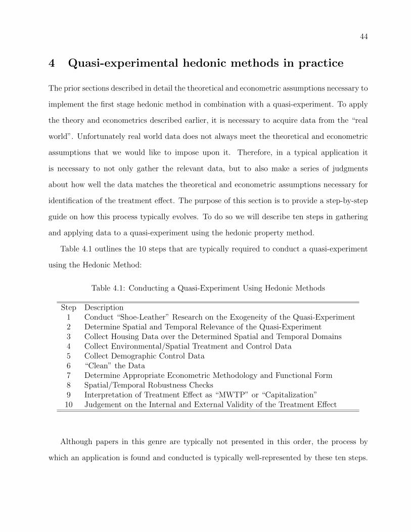
44
4 Quasi-experimental hedonic methods in practice
The prior sections described in detail the theoretical and econometric assumptions necessary to
implement the first stage hedonic method in combination with a quasi-experiment. To apply
the theory and econometrics described earlier, it is necessary to acquire data from the “real
world”. Unfortunately real world data does not always meet the theoretical and econometric
assumptions that we would like to impose upon it. Therefore, in a typical application it
is necessary to not only gather the relevant data, but to also make a series of judgments
about how well the data matches the theoretical and econometric assumptions necessary for
identification of the treatment effect. The purpose of this section is to provide a step-by-step
guide on how this process typically evolves. To do so we will describe ten steps in gathering
and applying data to a quasi-experiment using the hedonic property method.
Table 4.1 outlines the 10 steps that are typically required to conduct a quasi-experiment
using the Hedonic Method:
Table 4.1: Conducting a Quasi-Experiment Using Hedonic Methods
Step Description1 Conduct “Shoe-Leather” Research on the Exogeneity of the Quasi-Experiment2 Determine Spatial and Temporal Relevance of the Quasi-Experiment3 Collect Housing Data over the Determined Spatial and Temporal Domains4 Collect Environmental/Spatial Treatment and Control Data5 Collect Demographic Control Data6 “Clean” the Data7 Determine Appropriate Econometric Methodology and Functional Form8 Spatial/Temporal Robustness Checks9 Interpretation of Treatment Effect as “MWTP” or “Capitalization”10 Judgement on the Internal and External Validity of the Treatment Effect
Although papers in this genre are typically not presented in this order, the process by
which an application is found and conducted is typically well-represented by these ten steps.
45
The remainder of this section fleshes-out the importance of each step.
4.1 Determining exogeneity and spatial/temporal domains (steps
1-2)
An ideal environmental quasi-experiment will stem from an exogenous change in the quality
(or information about the quality) of an environmental attribute that is reflected in housing
prices. The first step in conducting a quasi-experiment using the hedonic method is to conduct
“shoe-leather research” (Angrist and Krueger, 2001) that documents the exogeneity of the
change. In an ideal quasi-experiment the change happens at an unexpected discrete point in
time from the viewpoint of homeowners. The concern is that if the quality change was expected
by homeowners, then these expectations blur the timing of when the change in environmental
quality will likely be reflected in housing prices. However, if it can be documented that
homeowners were not expecting the change, then it is easier to argue that differences in
housing prices before and after the environmental can be interpreted causally.
Changes in environmental attributes of housing fundamentally occur in time and space.
Furthermore, every housing transaction takes place within a temporal and spatial context.
Thus, it is crucial to understand the timing of the exogenous environmental change and the
spatial influence that that change has in the housing market. Depending on the environmental
change, location of the temporal and spatial bounds of the analysis can be trivial, or involve
a substantial amount of additional research. Understanding the temporal and spatial bounds
of the analysis early on in the research process can save vast amounts of time in collecting the
data described in section 4.2.
46
4.2 Collecting housing, treatment & control, and demographic data
(steps 3-5)
A key issue with a hedonic study is determining what constitutes a “housing market”. When
one decides to study a policy of interest, data is gathered for a specific housing market and
then analyzed using a variety of methods to assess the policy impact via changes in housing
prices. A key issue is how one defines the “relevant” housing market.17 Traditional studies use
housing sales only and provide a judgement for the appropriate housing market. However, if
this definition were in doubt an alternative attempt to validate the market would be to survey
home buyers and ask them about areas they see as comparable to where they currently live.
If one defines a housing market that is too small, then the lack of observations may lead
to less precise estimates of the pertinent hedonic parameters. Alternatively, if one defines a
housing market that is too large then house sales are being included in the analysis where
the policy change was not part of the information set and, depending on the expected impact
of the policy, will result in over/under estimation of the policy’s affect. In prospect, internal
validity is threatened when the housing market is too large and external validity is threatened
when the housing market is too narrowly defined.18
The distinction of a specific housing market needs to balance between where buyers/sellers
start to take on different preferences, where the policy will have no impact, when the policy
does not enter into the information set, and where transaction costs prohibit adjustment to
the policy. Each of these features has important implications for correct interpretation of a
treatment effect estimated from a quasi-experimental study.
One can think of the definition of the appropriate housing market as akin to the bias-
variance tradeoff that occurs in econometrics. For a smaller housing market, one increases
17This also raises issues in terms of the true impact of the policy if homeowners cannot move (due totransaction costs) to adjust accordingly to the policy change.
18Internal validity is defined as the ability of a model to predict within sample, while external validity isthe ability of a model to predict out of sample.

47
variance (on MWTP estimates) but decreases bias. For a larger housing market one decreases
variance but increases bias. What is needed is to strike the right balance between bias and
variance. Unfortunately, no metric exists for determining the extent of the housing market
as it does in econometrics (such as mean square error). This is purely a judgement call that
requires a careful analysis of the available data, the policy in question, and the estimation
methods being used.
Once an exogenous environmental change is discovered and the spatial and temporal rel-
evance of that change have been determined, there are three types of data that researchers
typically compile in order to analyze a quasi-experiment in the housing market. They are: (i)
housing data, (ii) environmental data and (iii) demographic data. Each of these data must
provide the spatial and temporal resolution needed to identify the causal effect that is being
studied. Acquiring data that spans the temporal and spatial area that encompasses an ex-
periment has been a major obstacle to this type of research in the past. However, with the
advent of GIS and the reduced cost of electronically archiving data, the availability of these
data has grown tremendously over the past decade. This section provides a broad look at how
these three types of data can be acquired for areas in the United States and how they can be
combined in preparation for quasi-experimental analysis.
4.2.1 Housing data
In the literature, studies have typically acquired housing data from three different sources: (i)
transaction and assessment data, (ii) multiple listing service data and (iii) census and survey
data. Each data source has its strengths and weaknesses, such that one data source may be
more appropriate for a given analysis than another. Furthermore, some of these data sources
are easier to acquire than others. Little time has been spent in the literature discussing these
different types of housing data, their accuracy, how they can be combined, and where they

48
might be acquired.19 Therefore, we discuss these topics here in hopes that it will aid the
research process in this area.
Currently, the most commonly used of the three data sources is transaction and assessment
data. Transaction data is often available from local governments because localities record deed
transfers. The data recorded on the deed typically includes the property address, selling price
and sale date. Assessment data is also available from local governments who assess properties
for tax purposes. This data often includes structural characteristics of the property, zoning and
other land use characteristics, and assessment values. Increasingly, towns, cities and counties
archive this data electronically and assign a unique id to each property. It is now common
for tax assessment offices of these localities to link the transaction data to the assessment
data and provide these data to interested parties on CD for a nominal fee.20 There are also
data vendors that collect this information from localities, repackage it, and sale the data to
interested parties.21
One of the primary strengths of this data source is the detail it provides on the structural
and land characteristics of a property. Also, since transaction data is collected over time, one
can use the data to conduct a repeat-sales model or use pooled cross-sections to understand the
impact of a quasi-experiment. Furthermore, with street addresses or a GIS parcel file, one can
map each property to a point in space so that it can be related to urban and environmental
features using a GIS software. A weakness of this data is that it takes time and effort to
understand the way that a particular assessment office codes certain variables, and to clean
the data for various problems such as non-arm’s-length transactions and changes in property
quality between assessments (a discussion of the importance of data cleaning is provided in
19Pollakowski (1995) is a dated but useful exception.20When transaction prices are not available, it is possible to use the assessed values as proxies for transaction
prices. However, the reliability of this procedure depends on how well the assessed values approximate whatthe properties would have been transacted for. Thus it is important to understand the assessor’s process ofdetermining assessed values if assessed values are to be used in the analysis.
21Some of these companies include: Dataquick, Transamerica, Experian, and others.
49
section 4.3).
Another source of housing data comes from Realtor associations. Realtor associations,
on local or sometimes regional scales, often create a shared database called a multiple listing
service (MLS). The MLS allows realtors in the area to list the properties they are representing
so that it can be easily seen by all the other brokers and realtors in the area. Given that the
MLS collects standard information about a property such as address, structural characteristics,
and the listing price of the house, it allows buyers and their agents to search for homes in the
area based on a price range, or size of house. The database also records the date of when a
property was listed and when the property was sold.
One of the strengths of MLS data is that it provides information on how long a property was
on the market before it sold. This “days-on-market” information is not available in any of the
other housing data sources. Days-on-market is another margin by which one can understand
the impact of a quasi-experimental change on housing prices (see Huang and Palmquist, 2001).
One of the weaknesses of MLS data is that only homes sold using a realtor with access to the
MLS are listed in the database. Another weakness of the MLS is that realtors are typically
not required to fill in all of the fields within the MLS system. For example, some realtors
may consistently input information on the type of flooring in the house whereas others may
not. Furthermore, it is likely that realtors are selective on the attributes of a house that they
describe on the MLS so as to promote the positive features of the house. This form of selection
bias can potentially hamper an analysis.
Another source of housing data comes from census and survey data collected by the gov-
ernment. There are three primary sources of census and survey data that are collected by the
federal government on a periodic basis that researchers have used. The U.S. Decennial Census
Summary File 3 (SF3) Sample Data, which is collected every ten years, asks households some
housing related questions that could be used for a quasi-experimental hedonic analysis. For
example, households provide information on their perceived value of their house that could
50
be used as “prices”. Households also provide some limited information on housing attributes
such as the number of rooms, number of bedrooms, and whether or not a house has plumbing
facilities.
One obvious difficulty with this data is that the “prices” are not actual transaction prices
but a homeowner’s best guess as to what their house would sell for. If housing prices are
appreciating or depreciating rapidly, the best guesses could potentially be skewed away from
market prices. Another difficulty with this data is that they are available only every ten years
and therefore would not work for many types of quasi-experiments. Likewise, the housing
attributes are limited compared to other housing data sources. Finally, the unit of observation
is not a house as conceptualized in the hedonic model, but a geographic unit such as a block-
group or a census tract. This aggregation could potentially change the interpretation of
hedonic estimates. A strength of the SF3 as a housing data source, is that it is very easy
to acquire at geographic scales larger than the base unit of observation. It can be used for
quasi-experiments that occur between the 10 year spans as long as the impact of the exogenous
event is likely to be larger than the unit of observation (i.e. block group).
A second census data source that has been used in hedonic research is the 5-Percent Public
Use Microdata Sample (PUMS) files. These files have census data for individual characteristics
of a 5 percent sample of housing units located within Public Use Microdata Areas (PUMAs).
A PUMA contains a minimum population of 100,000 people. The value of this data relative to
the SF3 file is that the unit of observation is an individual housing unit, and the information
about the housing unit is of a more detailed variety. However, this increased resolution in
housing characteristics comes at the cost of a loss of spatial precision on where the housing
units are at. This is because PUMAs are mostly at the spatial aggregation of a county or
multiple counties.22
22In highly populous areas there are multiple PUMAs within a county, but even these PUMAs are still muchmore highly aggregated than block groups or even census tracts.
51
The final census data source that has been used in hedonic research is the American
Housing Survey (AHS). The AHS is a survey of a representative sample of homes across the
entire U.S and across specific metropolitan areas. Part of the national sample is a true panel of
houses. The survey elicits detailed information about demographics, structural characteristics,
the owner’s estimate of the homes value, and transaction prices if the home was purchased
in the previous 12 months. There are two primary difficulties with using the AHS for quasi-
experimental analysis. First, because of sample size issues the government does not release
detailed information on the geographic location of the houses to protect the identities of survey
respondents. Therefore, the researcher only knows where a house is located down to the state,
metropolitan area, or sometimes a zone within a metropolitan area. The second difficulty is
that the national survey is done every other year, and the metropolitan survey is done every
3-4 years. An advantage of the AHS data is the detailed information on the people who live
in the homes and detailed information on the quality of the homes that typically cannot be
obtained anywhere else.
Another data issue is whether to use repeat sales data for a group of selected houses
or an aggregated data set that constitutes generic home sales over some specified period.
There are several reasons both for and against using repeat sales. Typically, repeat sales data
are constructed from transaction price data as opposed to list price data which increases the
likelihood of obtaining prices closer to what the buyer paid/seller received. Also, as mentioned
previously, since the houses transacting are observed at various points in time it is easier to
control for unobserved heterogeneity, especially if this heterogeneity is not changing over time.
Even with these appealing features of using repeat sales data there are reasons for not
using this type of approach. First, these methods only provide insight into price changes.
Price levels for an entire MSA or for some smaller segments is ignored with repeat sales data.
Second, sample sizes can be reduced significantly since homes that only sell once over the
study period are dropped from the dataset. Lastly, houses that have sold repeatedly over the
52
time period may not reflect actual market patterns or may be systematically different from
the majority of units that are available in the market.
While there are reasons for both using and avoiding repeat sales data in an experimental
design, we point out that for any particular empirical application care and judgement on
behalf of the researcher is warranted. Only the researcher can know, given the data at hand,
the time frame, and the policy question of interest if using generic home sales or repeat sales
data are valid to study a policy change.
4.2.2 Environmental data
There are many potential places to acquire environmental data that can be linked to hous-
ing data. With the advent of GIS, many government and private agencies produce spatial
information on various environmental attributes. Often using an internet search engine by
inputting key words on the environmental attribute, the place you are conducting your study
and a GIS format such as “shapefile”, can help one to find the information. However, if that
does not succeed, the next place to look when conducting a hedonic analysis is typically the
government agency that corresponds to the scale of the study. For example, if one is con-
ducting a hedonic analysis on a city-wide scale, then one should approach the city or county
governments responsible for that city to find out what GIS data they have. If that fails to
produce the information required, then one can look to state or federal government agencies
that are most likely to produce the information required. For example, www.nationalatlas.gov
houses a variety of environmental datasets in shapefile format.
4.2.3 Demographic data
Demographic data is typically taken from the Decennial Census Summary File 3. Variables
commonly used in hedonic analyses include: percent non-white, median house values, median
time-to-work, percent of population under 18, and percent of housing that is owner occupied.

53
Just like the housing data in the Decennial Census, the finest geographic resolution of the
public version of this data is available only at the block group or census tract level. Thus
when this information is attached to individual houses in the housing data, one is attaching
a summary measure of that houses “neighborhood” where that neighborhood is defined as a
block group or census tract.
One difficulty with using the SF3 information is that it is only collected every 10 years.
In a quasi-experiment if it is thought that neighborhood demographics are changing over
the time horizon of the quasi-experiment, then the best one can do with the census data is
to interpolate the changes in demographics over the 10 year span and attach year specific
interpolated measures to when a particular house sold. One must weigh the tradeoff of in-
troducing this measurement error with the cost of acquiring some other form of demographic
information. Another concern of interpolating the census information over time is the fact
that block-group and census tract boundaries often change between censuses. When this hap-
pens, the interpolation process becomes much messier since one must spatially weight the
data between censuses. Fortunately, there are now some products such as the “Neighborhood
Change Database” produced by Geolytics that has already dealt with the challenges of spatial
weighting. For example, the Geolytics product provides Census data from 1970, 1980, 1990
and 2000 at the census tract level where the data is consistently defined to the 2000 Census
tract boundaries.
4.3 Cleaning of the housing data (step 6)
Housing data, whether it was acquired from the assessor’s office, the multiple listing service
or the census, typically requires efforts to eliminate errors or outlying observations before it
can be used in a quasi-experimental analysis. In the literature, it is sometimes difficult to
understand exactly how authors cleaned their data because it is often relegated to a short
54
footnote or not included at all. Yet, the assumptions made in the cleaning process can
ultimately influence the results from a study. Therefore, caution and good judgment should
be used as one prepares the housing data for the analysis.
One typical problem with many housing datasets is standard data entry errors. It is
important to thoroughly explore the data for outliers in the key variables used in the analysis.
Another issue that arises with assessor datasets is that sales prices include both “arms-length”
and “non-arms-length” sales. Non-arms-length sales include the homes that were sold at a
large discount to relatives, as part of another business transaction, and a variety of other
circumstances which likely cause the sales price to differ from a true market price of a home.
Because county assessor’s often use housing prices to determine their assessments, they often
include a variable that helps to sort out the arms-length transactions from all the others.
This is an important variable to understand so that a determination can be made on which
transactions should be included in the analysis. It is of course possible that an assessor may
label some homes that were greatly affected by the environmental change that is being studied
as non-arms-length sales. This then requires direct communication with the assessor’s office
to determine.
A final data cleaning issue is determining the best way to geo-locate housing transactions.
A common way of doing this is to use a GIS software in combination with road network files to
“geo-code” the housing addresses provided with a housing dataset. This geo-coding technique
results in an estimated latitude and longitude of each house. However, it can be expected that
acquiring the parcel files for a county where the housing data is located and then estimating
the centroid of each parcel provides a latitude and longitude with less measurement error for
housing transactions in the dataset.
While many papers in the hedonic literature discuss the robustness of their results to
theoretical and econometric assumptions, it is uncommon to devote paper space to discussing
the robustness of results to the assumptions made in the cleaning process. Nonetheless, it is
55
the responsibility of the researcher to determine if changes in the way the data is cleaned do
matter. Therefore, at a minimum, enough detail should be provided about the data cleaning
process that replication can take place by other researchers.
4.4 Choosing functional form and spatial robustness checks (steps
7-8)
As described earlier in this chapter, the hedonic price function is in general, nonlinear without
a closed form solution. Nonetheless, most empirical studies treat linearity as a maintained as-
sumption. The justification for this practice often stems from an influential paper by Cropper,
Deck and McConnell (1988). In their paper, a Monte Carlo analysis was performed on the
accuracy of certain functional forms on predicting the MWTP of various housing attributes.
The primary result from this paper was that when all housing characteristics are observed by
the researcher, more flexible functional forms such as the linear Box-Cox and the quadratic
Box-Cox models perform best in predicting MWTP for cross sectional analysis. However,
when one of the characteristics is unobserved or replaced by a proxy, the linear, semi-log,
and double-log all outperform the quadratic Box-Cox. Because of the widespread concern
for omitted variable bias, especially in cross-sectional models, the subsequent literature has
typically used these simpler linear functional forms without rigorous specification tests.
In the twenty years that have elapsed since the Cropper, Deck and McConnell (1988)
study, there have been significant changes in the way hedonic price functions can be esti-
mated. Furthermore, in a quasi-experimental analysis, omitted variables can be partially
mitigated through spatial and temporal fixed effects. With these and other issues in mind,
a recent working paper by Kuminoff, Parmeter and Pope (2009), have conducted a Monte
Carlo simulation that updates and extends the simulations of Cropper, Deck and McConnell.
These simulation studies can serve as guidance for empirical specification, but some effort to

56
analyze the robustness of the quasi-experimental results to changes in functional form, should
occur for any given application. Also, given that what one is typically interested in is not the
slope of the hedonic price function at a particular point but the difference in slopes at two
points, it is not clear how functional form choice influences this metric. It may turn out that
the method best suited for measuring the slope is perhaps not the best method to estimate a
difference between slopes.23
4.4.1 Controlling for time and space confounders
To this point in our discussion we have highlighted the process of gathering data and employ-
ing a valid identification strategy used by researchers conducting natural and quasi-natural
experiments. What warrants further discussion are the implicit assumptions made by quasi-
experimental researchers and the implications of empirical decisions made during estimation.
To begin, lets consider our underlying relationship between home prices, observable charac-
teristics, and treatment status,
Pi = m(Xi, D1i) + εi, for i = 1, . . . , n. (47)
Equation (47) forms the basic representation between home prices and other data used in
current quasi-experimental settings. Typically, aside from controlling directly for neighbor-
hood and physical characteristics, there are two other components that need to be addressed
to make sure that the above treatment methodologies are adequately capturing causal treat-
ment effects: time and space. Even though time and space dummies can be included with
relative ease in any estimation of a conditional mean, the subtleties of these impacts are often
overlooked.
23Also, when one uses repeat sales, traditional approaches do not use the functional form of the hedonicequilibria and so it is not clear how evaluation of a policy is influenced. This would be a fruitful avenue forresearch.
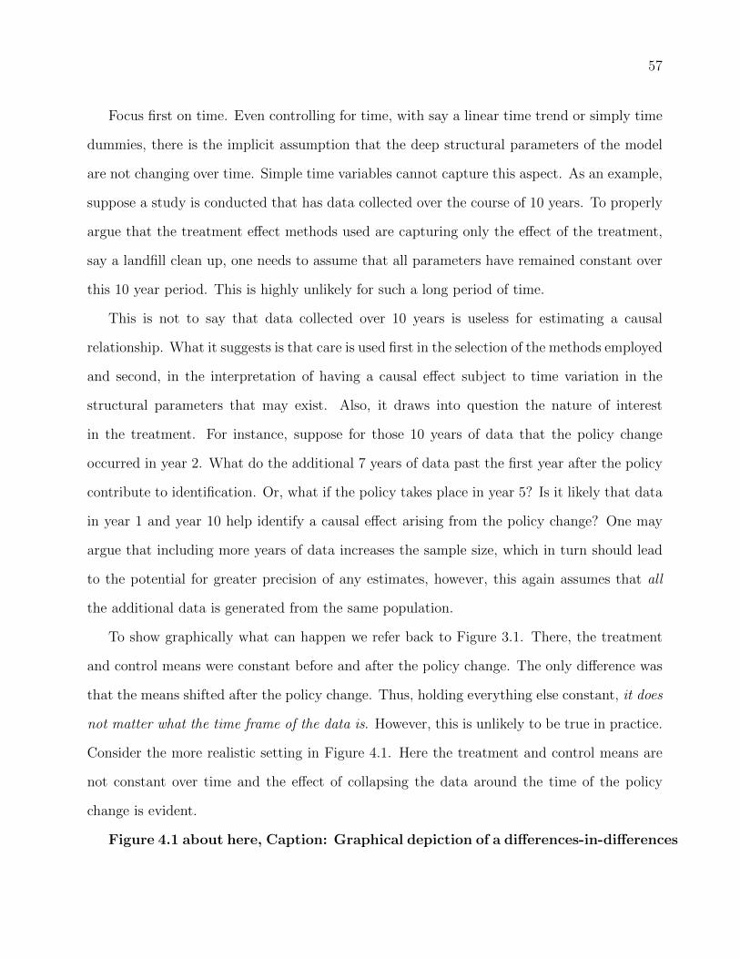
57
Focus first on time. Even controlling for time, with say a linear time trend or simply time
dummies, there is the implicit assumption that the deep structural parameters of the model
are not changing over time. Simple time variables cannot capture this aspect. As an example,
suppose a study is conducted that has data collected over the course of 10 years. To properly
argue that the treatment effect methods used are capturing only the effect of the treatment,
say a landfill clean up, one needs to assume that all parameters have remained constant over
this 10 year period. This is highly unlikely for such a long period of time.
This is not to say that data collected over 10 years is useless for estimating a causal
relationship. What it suggests is that care is used first in the selection of the methods employed
and second, in the interpretation of having a causal effect subject to time variation in the
structural parameters that may exist. Also, it draws into question the nature of interest
in the treatment. For instance, suppose for those 10 years of data that the policy change
occurred in year 2. What do the additional 7 years of data past the first year after the policy
contribute to identification. Or, what if the policy takes place in year 5? Is it likely that data
in year 1 and year 10 help identify a causal effect arising from the policy change? One may
argue that including more years of data increases the sample size, which in turn should lead
to the potential for greater precision of any estimates, however, this again assumes that all
the additional data is generated from the same population.
To show graphically what can happen we refer back to Figure 3.1. There, the treatment
and control means were constant before and after the policy change. The only difference was
that the means shifted after the policy change. Thus, holding everything else constant, it does
not matter what the time frame of the data is. However, this is unlikely to be true in practice.
Consider the more realistic setting in Figure 4.1. Here the treatment and control means are
not constant over time and the effect of collapsing the data around the time of the policy
change is evident.
Figure 4.1 about here, Caption: Graphical depiction of a differences-in-differences
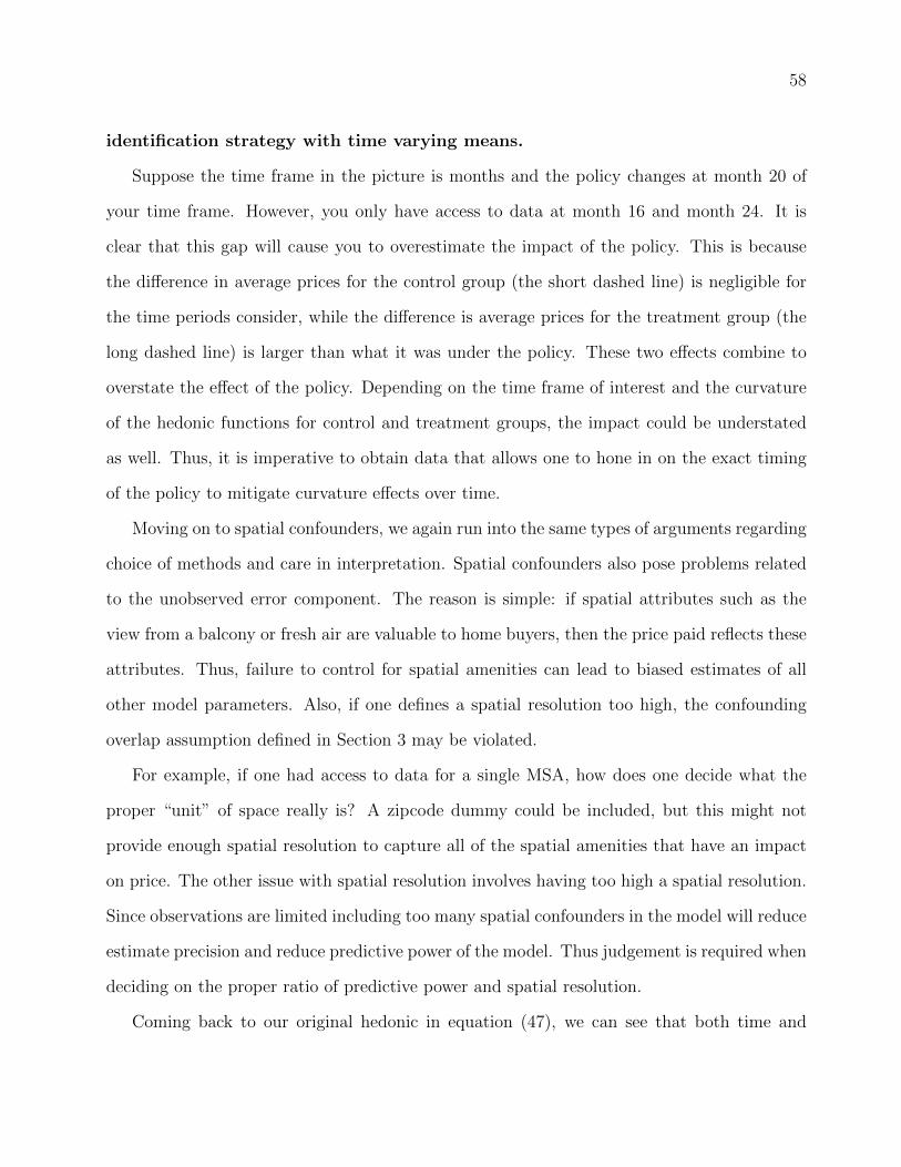
58
identification strategy with time varying means.
Suppose the time frame in the picture is months and the policy changes at month 20 of
your time frame. However, you only have access to data at month 16 and month 24. It is
clear that this gap will cause you to overestimate the impact of the policy. This is because
the difference in average prices for the control group (the short dashed line) is negligible for
the time periods consider, while the difference is average prices for the treatment group (the
long dashed line) is larger than what it was under the policy. These two effects combine to
overstate the effect of the policy. Depending on the time frame of interest and the curvature
of the hedonic functions for control and treatment groups, the impact could be understated
as well. Thus, it is imperative to obtain data that allows one to hone in on the exact timing
of the policy to mitigate curvature effects over time.
Moving on to spatial confounders, we again run into the same types of arguments regarding
choice of methods and care in interpretation. Spatial confounders also pose problems related
to the unobserved error component. The reason is simple: if spatial attributes such as the
view from a balcony or fresh air are valuable to home buyers, then the price paid reflects these
attributes. Thus, failure to control for spatial amenities can lead to biased estimates of all
other model parameters. Also, if one defines a spatial resolution too high, the confounding
overlap assumption defined in Section 3 may be violated.
For example, if one had access to data for a single MSA, how does one decide what the
proper “unit” of space really is? A zipcode dummy could be included, but this might not
provide enough spatial resolution to capture all of the spatial amenities that have an impact
on price. The other issue with spatial resolution involves having too high a spatial resolution.
Since observations are limited including too many spatial confounders in the model will reduce
estimate precision and reduce predictive power of the model. Thus judgement is required when
deciding on the proper ratio of predictive power and spatial resolution.
Coming back to our original hedonic in equation (47), we can see that both time and
59
spatial confounders make up the composition of our attribute matrix Xi. So mathematically,
when we are concerned with time and space what one needs to consider of is that the hedonic
function is either not changing over time/space, or that an adequate resolution is imposed
so that any changes are parsed out of the hedonic calculation. Using the notation mts(·) to
reference the hedonic function at time t for spatial area s we either assume that,
mts(Xi, D1i) = mrl(Xi, D1i), for i = 1, . . . , n, t, r = 1, . . . , T, and s, l = 1, . . . , S, (48)
if we are not controlling for time and space, or
mts(Xi, D1i, At, As) = mrl(Xi, D1i, Ar, Al), for i, j = 1, . . . , n, t, r = 1, . . . , T, and s, l = 1, . . . , S,
(49)
where At and Ar are time confounders and As and Al are spatial confounders all entering in
directly to the hedonic function.
We do not suggest making the assumption that the hedonic function across time and space
is identical unless (equation (48)) one has carefully created a dataset that has a short time
span and controls for various spatial amenities directly in the attribute matrix. More likely,
time and spatial resolution matrices will need to be created and entered directly into the
hedonic estimation as suggest in equation (49).
4.5 Interpretation of estimates, internal and external Validity (steps
9-10)
Once the average treatment effect has been estimated the results should be used to discern
policy prescriptions. This is a difficult task as it requires careful interpretation of what has
been estimated, and how it should be used both within and out of the housing area of study.
As an example, should one blindly use a treatment effect for air quality obtained in Orange
60
county, California to make recommendations for a change in air quality in Orange county,
New Jersey? This question gets at the interaction between the use of quasi-experiments and
benefit transfers.24
As discussed earlier, a researcher must be careful in interpreting an average treatment effect
as a MWTP and if he/she cannot be confident in this assertion then considering this estimate
as a capitalization rate requires a different type of policy recommendation. To properly use
a treatment effect the researcher needs to address which assumptions may be violated. For
example, suppose one has a clean identification strategy but data availability does not allow
her to place a narrow time window around the natural event. The onus then falls on the
researcher to be able to explain how likely the wide time gap is to impact the treatment effect.
Also, the impact of the change providing the natural experiment is important to document to
aide in determination of the estimate as a MWTP as opposed to an AMWTP.
Aside from issues surrounding internal validity (here internal validity is taken to mean
that the estimated treatment effect is a valid estimate of the actual treatment effect) external
validity of a quasi-experiment is an important consideration as well. Suppose one was inter-
ested in water quality valuation in San Diego, California but no natural experiment existed to
determine the effect. However, if a water quality quasi-experimental study was done in Miami,
Florida, a natural question to ask is how similar the two treatment effects are. Both cities
have nice weather, are on the ocean, and have international airports. However, the researcher
would still need to argue that the assumptions used in the Miami study were valid for the San
Diego area. If they were not then the Miami treatment effect is an unacceptable candidate to
value water quality in San Diego. This type of interest is known as external validity (being
able to argue that the estimated treatment effect in one place is valid for an entirely different
location).
If a quasi-experiment is undertaken that is too narrowly focused, then external validity is
24For more on benefit transfers see Boyle and Bergstrom (1992).
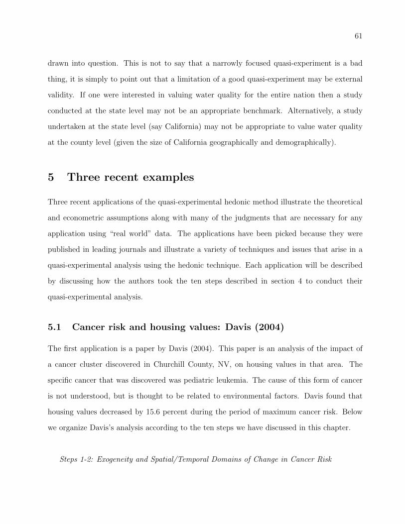
61
drawn into question. This is not to say that a narrowly focused quasi-experiment is a bad
thing, it is simply to point out that a limitation of a good quasi-experiment may be external
validity. If one were interested in valuing water quality for the entire nation then a study
conducted at the state level may not be an appropriate benchmark. Alternatively, a study
undertaken at the state level (say California) may not be appropriate to value water quality
at the county level (given the size of California geographically and demographically).
5 Three recent examples
Three recent applications of the quasi-experimental hedonic method illustrate the theoretical
and econometric assumptions along with many of the judgments that are necessary for any
application using “real world” data. The applications have been picked because they were
published in leading journals and illustrate a variety of techniques and issues that arise in a
quasi-experimental analysis using the hedonic technique. Each application will be described
by discussing how the authors took the ten steps described in section 4 to conduct their
quasi-experimental analysis.
5.1 Cancer risk and housing values: Davis (2004)
The first application is a paper by Davis (2004). This paper is an analysis of the impact of
a cancer cluster discovered in Churchill County, NV, on housing values in that area. The
specific cancer that was discovered was pediatric leukemia. The cause of this form of cancer
is not understood, but is thought to be related to environmental factors. Davis found that
housing values decreased by 15.6 percent during the period of maximum cancer risk. Below
we organize Davis’s analysis according to the ten steps we have discussed in this chapter.
Steps 1-2: Exogeneity and Spatial/Temporal Domains of Change in Cancer Risk
62
Although little time was spent discussing the exogeneity of the change in cancer risk, the
paper does document the discontinuous change in newspaper articles that begins in the middle
of the year 2000. Given that Churchhill County had no prior history of pediatric leukemia
before the late 1990’s and given the lack of media attention prior to the middle of the year
2000, it does seem reasonable that this event can be viewed as exogenous from the perspective
of homeowners within the county. Nonetheless, the event was not perfectly discontinuous
in time or space and therefore this should be considered in the design of the identification
strategy.
In the paper Davis does use several non-discontinuous measures of change in cancer-risk
over time in his empirical specifications. However, cancer risk is assumed to be uniform across
Churchhill County, but discretely different at neighboring Lyon County which is used as a
control group in the analysis. Davis does make this assumption explicit when he states on
pg. 7, “However, their close proximity to the highly publicized cases in Churchill County may
have caused them to increase their own perceptions of risk. If this is the case the estimated
difference in risk between the two counties will be overstated.”
The spatial unit of analysis in the paper are the two counties (Churchill and Lyon) that
are used as the treatment and control counties. Figure 5.1 shows these counties in relation
to one another and the other counties in Nevada. A question that arises from this figure
is whether or not the spatial heterogeneity in cancer risk should be considered given the
large area encompassed by the two counties. Further discussion or graphical depiction of
where the housing sales occurred would have been useful for the identification strategy. If
the cancer cluster occurred closer Churchill county’s border with a county other than Lyon,
then using Lyon county as the control group may be inappropriate. Also, Lyon county has a
much higher population density than Churchill county over the time frame of Davis’s analysis.
63
Figure 5.1 about here, Caption: Counties in the state of Nevada.
Steps 3-6: Collecting and Cleaning Housing and other Data
The housing data for the paper was collected from the Churchill and Lyon County Assessors
offices. This data was used not only for the ultimate analysis, but was also used to construct
county price indices to determine if Lyon County is indeed a reasonable control group for
Churchhill County. It appears that some data cleaning took place as documented in footnote
1 on page 8. Here it says that “Three percent of sales were excluded from the analysis due
to missing values or miscoding.” The footnote then documents how many observations were
excluded from the analysis for the construction year missing, sales price missing, etc. etc.
There was no mention of the issue of arms-length sales. Furthermore, since this is a county
wide analysis, no effort was made to geo-code the housing information.
Davis also collects demographic characteristics from the 2000 census and employment
statistics from the Bureau of Economic Analysis. These are also used to determine if Lyon
County can act as a reasonable control group (counts of newspaper articles about the cancer
cluster were also collected from Proquest). Again, the distribution of demographic charac-
teristics of the two counties, relative to the location of the cancer cluster, is important for
validating the treatment effect when using Lyon county as the control.
Steps 7-8: Hedonic Functional Form and Robustness Checks
Davis uses pooled cross-sections and difference and difference estimation to identify the
impact of the occurrence of the cancer cluster on housing prices. Using the simple group mean
DD discussed previously, Davis finds that the change in house values in Churchill county after
the cancer cluster was found was roughly -4% while home values increased by 4% in Lyon
county after the cancer cluster was found. Taken together, the generic DD estimator suggests
64
that home values decreased by almost 8% after the cancer cluster was announced.
However, Davis rightly notes that over the period of the cancer cluster forming the com-
position of houses has changed as well. Thus, he estimates a more rigorous DD model to
account for this additional housing heterogeneity. The empirical model includes a limited set
of housing controls, home-specific fixed effects, county by time fixed effects, and a measure
of cancer risk. The functional form of the hedonic price function is semi-log. The baseline
regression has the form
pijt = xijtβ + γRISKjt + αi + λjt + εijt, (50)
where i indexes homes, j indexes the county (Lyon or Churchill), and t indexes time. No justi-
fication is given for using the semi-log model. Estimating this model via OLS and least-squares
dummy variables (LSDV) Davis obtains estimates of γ that suggest the housing differential
between Churchill and Lyon is even larger than the basic DD. OLS provides an estimate of
nearly 16% while LSDV estimates the differential at 14%. The heterogeneity of the price
impact over different sized homes is explored, but not for homes located in different areas
within the county.
The robustness of the results to location, how the data was cleaned and the functional
form of the data were not considered. Calculations performed by the authors suggest that
introducing basic nonlinear versions of RISK, such as a quadratic term, do not impact the
raw estimates, suggesting robustness of the DD treatment effect to how RISK enters the
model.
Steps 9-10: Interpretation and Validity of Treatment Effect
The estimates are interpreted as reflecting the MWTP of households to reduce the risk of

65
cancer within the household.25 However, it could be argued that the change in risk perceptions
was so large, given the rapid onset of the cancer cluster that what Davis has really estimated
is AMWTP. Therefore, some caution is warranted when trying to value people’s perceptions
of risk based on such a nonmarginal change.
Overall, the Davis (2004) paper is an excellent illustration of how the hedonic technique
can be combined with a quasi-experiment to uncover the impact of an important housing
attribute, health risk, on housing prices. Nonetheless, there were still places where judgments
that took place specific to the application could have been explored for their impact on the
final results in the paper. For example, from a spatial perspective the analysis was conducted
at the county level for two counties: Churchill (treated county) and Lyon (control county).
Lyon county only shares a small fraction of Churchill’s border with it, and is more densely
populated (Churchill has 5 people / square mile, Lyon has 23/square mile) some sensitivity to
the chosen control group would be useful. Furthermore, cancer risk was treated as uniformly
distributed within the county. However, with such a large county, it would be potentially
important to understand the heterogeneity of the housing price impact by where the cancer
occurrences occurred within the county.
5.2 Air quality and housing values: Chay and Greenstone (2005)
The second application used to illustrate the quasi-experimental approach to hedonics is de-
scribed in Chay and Greenstone (2005). In their paper they use amendments to the Clean
Air Act that caused quasi-random reductions in air pollution to estimate the impact of air
quality on housing prices. They found that a 1 microgram per cubic meter reduction in total
suspended solids (TSP) resulted in approximately a 0.20 to 0.40 percent increase in property
values. This estimate of the impact of air quality on housing prices is significantly larger than
25See his footnote 2 for more discussion on the interpretation of his estimates.
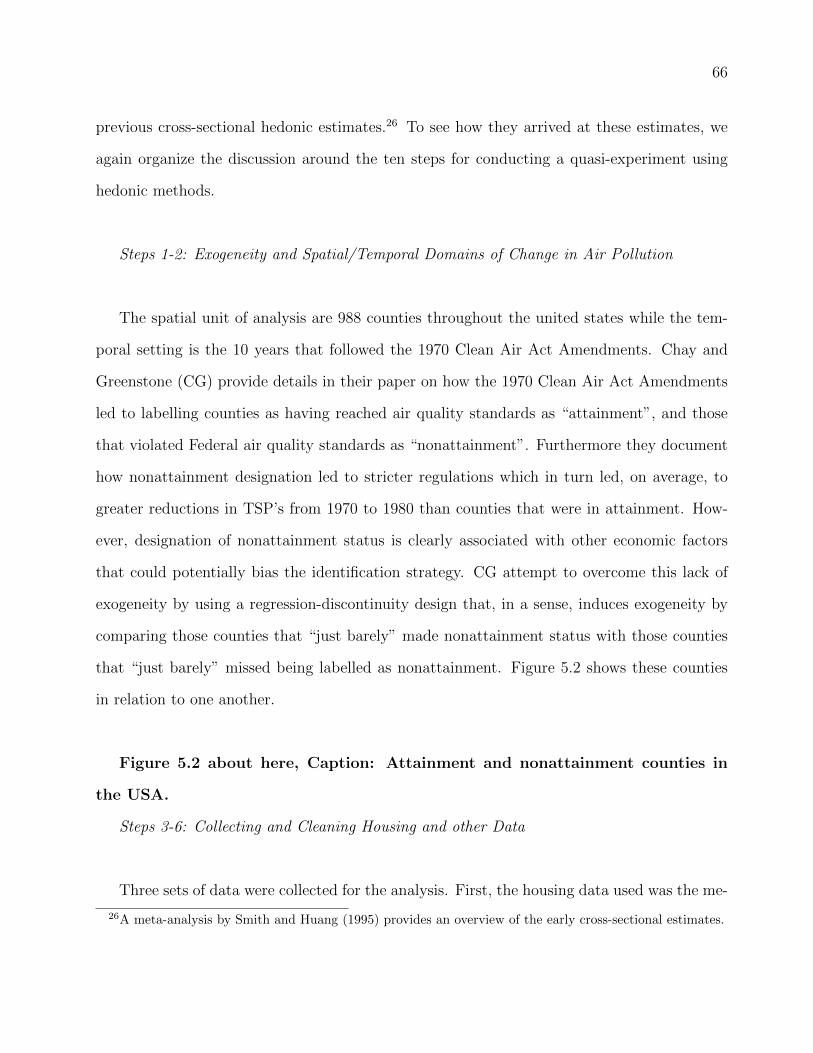
66
previous cross-sectional hedonic estimates.26 To see how they arrived at these estimates, we
again organize the discussion around the ten steps for conducting a quasi-experiment using
hedonic methods.
Steps 1-2: Exogeneity and Spatial/Temporal Domains of Change in Air Pollution
The spatial unit of analysis are 988 counties throughout the united states while the tem-
poral setting is the 10 years that followed the 1970 Clean Air Act Amendments. Chay and
Greenstone (CG) provide details in their paper on how the 1970 Clean Air Act Amendments
led to labelling counties as having reached air quality standards as “attainment”, and those
that violated Federal air quality standards as “nonattainment”. Furthermore they document
how nonattainment designation led to stricter regulations which in turn led, on average, to
greater reductions in TSP’s from 1970 to 1980 than counties that were in attainment. How-
ever, designation of nonattainment status is clearly associated with other economic factors
that could potentially bias the identification strategy. CG attempt to overcome this lack of
exogeneity by using a regression-discontinuity design that, in a sense, induces exogeneity by
comparing those counties that “just barely” made nonattainment status with those counties
that “just barely” missed being labelled as nonattainment. Figure 5.2 shows these counties
in relation to one another.
Figure 5.2 about here, Caption: Attainment and nonattainment counties in
the USA.
Steps 3-6: Collecting and Cleaning Housing and other Data
Three sets of data were collected for the analysis. First, the housing data used was the me-
26A meta-analysis by Smith and Huang (1995) provides an overview of the early cross-sectional estimates.

67
dian self-reported housing values reported in the 1970 and 1980 decennial census of population
and housing for the 988 counties used in the analysis. Data on county characteristics including
economic demographic, housing, tax, and neighborhood variable controls was also obtained
from primarily census information. They also collected TSP information at the county level
from 1969-1980 from the U.S. Environmental Protection Agency. It is this data that was used
to re-construct the attainment-nonattainment status variable.
Steps 7-8: Hedonic Functional Form and Robustness Checks
The primary results in the paper come from a semilog hedonic form that is first differ-
enced at the county-level between 1970 and 1980. The first-differencing controls for time
constant county level effects. On the left hand side of the regression equation is the log of
the median self-reported property value in the counties and on the right hand side is a set
of observed county characteristics including economic, demographic, housing, tax, and neigh-
borhood variables in various forms. An indicator variable is created for those counties labeled
as nonattainment in the mid-1970’s and included in the right hand side as an instrument for
TSP’s. In the most tightly controlled regressions there are also indicator variables for differ-
ent spatial regions throughout the U.S. and the sample is restricted to 419 counties that were
“barely” labeled attainment or nonattainment.27
The basic regression of CG is
∆pj = ∆Xjβ + γ∆Tj + ∆εj, (51)
where j indexes county and Tj is a measure of air quality in each county. The estimator of
CG uses instrumental variables because it is assumed that both ∆pj and ∆Tj are correlated
27There are also some additional robustness checks on the timing of the TSP nonattainment status, as wellas random-coefficient models to test for sorting of households.
68
with ∆εj. To correct for this endogeneity bias, CG use an indicator that identifies those coun-
ties with abnormally high levels of suspended particulates. Their argument is that counties
with levels of suspended particulates in 1975 that were close to the level of being deemed an
attainment county were more likely to clean the air than those counties with levels very far
from this benchmark, thus resulting in the county’s status switching. In essence, CG use a
regression discontinuity idea to construct their instrument as opposed to having one in the
primary regression design. However, given that they have one endogenous variable and one
instrument, both procedures are equivalent.
Steps 9-10: Interpretation and Validity of Treatment Effect
CG call their estimates of the impact of TSP’s on housing prices an “average MWTP”.
In order for CG to claim they have a MWTP they assume that MWTP is constant over time
and space. Given the extent of their housing market (a national market) and the time gap
between successive estimates (10 years) this is a tough sell. Given the nonmarginal change in
air quality across counties, what CG have estimated is more closely related to a capitaliza-
tion rate than an AMWTP. Furthermore, other hedonic assumptions could have important
implications for the interpretation of the estimate derived in the paper on the impact of
air quality on housing prices. For example, are households fully informed about air quality?
If we are assuming a national hedonic model, is it reasonable to assume moving costs are zero?
The CG paper provides a nice illustration of some of the theoretical and empirical tradeoffs
that are made in quasi-experimental analysis using the hedonic model. CG suggest that pre-
vious cross-sectional estimates were likely contaminated by omitted variable bias from factors
such as per capita incomes, population densities and crime rates that may be correlated in
space with high levels of TSPs. They argue that the quasi-exogenous application of nonattain-
69
ment status to some counties due to the Clean Air Act, offers the potential to difference-away
much of the unobserved factors that plagued previous work. However, to implement their
approach they rely on county-level data rather than micro-level household data, and assume
there is a national housing market. Both of these assumptions are problematic in that they
diverge from theoretical underpinnings of the hedonic model, but are necessary to exploit the
nonattainment quasi-experiment.
By using county-level data, identification rests on comparisons across counties while the
variation within counties is ignored. The data available to CG is self-reported values of homes
and a limited set of housing characteristics taken from U.S. Decennial Censuses. Actual hous-
ing transaction prices would be preferred if there are systematic differences in how households
misreport their perceived home value across the country. Furthermore if the characteristics
of homes systematically changed differently across counties this could also bias the estimates.
Spatial fixed effects would appear to be useful to control for some of these unobserved dif-
ferences in markets across the U.S. CG include spatial fixed effects in their most carefully
controlled regressions, but the spatial fixed effects are very large; one for each of the 9 census
defined regions of the U.S.
5.3 Airport noise and housing values: Pope (2008a)
The third and final application to be discussed is a paper by Pope (2008a). This paper is an
analysis of the impact of an airport noise disclosure that sellers were required to give home-
buyers near the Raleigh-Durham International Airport (RDU) in Wake County, NC. The
discrete timing of the introduction of the disclosure is used as a quasi-experiment to analyze
the impact of the airport noise information given to buyers on housing prices. Pope finds that
the airport noise disclosure reduced the value of houses in high-noise areas by 2.9 percent.
He notes that this is a 37 percentage point increase in the implicit price of airport noise from

70
before the disclosure began occurring. We again explore how the ten steps we have discussed
in this chapter were used to arrive at the estimated impact on housing prices.
Steps 1-2: Exogeneity and Spatial/Temporal Domains of Change in Airport Noise Infor-
mation
The paper makes some effort to assure the reader that the airport noise disclosure require-
ment was an exogenous event from the perspective of homeowners. A section of the paper is
devoted to describing the chain of events that led to a state law that allowed RDU to require
homeowners to provide an airport noise disclosure to all prospective buyers. The airport noise
disclosure began being issued in March of 1997, and the paper argues that there was not
advance notice given to homeowners that may have led some owners to try and sale their
homes “early” to avoid the disclosure. Other information is given on how the disclosure has
been enforced by the real estate community and by an “airport noise officer” who verifies that
disclosures are being given.
The spatial unit of analysis are the housing sales (at exact latitude and longitude points)
surrounding RDU. This allows an exact matching of the spatial location of a house in relation
to the airport. In the most tightly controlled regressions in the paper, the analysis concen-
trates on the year before and the year after the airport noise disclosures commenced being
given by sellers to buyers. Figure 5.3 shows these areas and their relative location to RDU.
Figure 5.3 about here, Caption: Airport noise disclosure area.
Steps 3-6: Collecting and Cleaning Housing and other Data
The spatial and temporal domains of the change in airport noise information used to collect
71
the housing and other sources of data are a fairly straight-forward exercise in the paper. RDU
provided the author with a file that spatially references noise contour zones surrounding the
airport. It is sellers of houses in these same noise zones that are required to provide the
disclosure. A one mile buffer was created outside the outermost noise contour, and houses in
this area were used as a control group in the identification strategy. The temporal domain
of the analysis is housing sales in the spatial areas described above, several years before and
several years after the sellers were required to provide the disclosure.
The housing data for the paper is micro-level data collected from the Wake County Rev-
enue Department. There is only one line describing the cleaning of the housing data. It states
“Sales were screened to ensure that they were arms-length and to eliminate outlying observa-
tions.” The spatial information on the noise contours was collected as described above, and
neighborhood control variables were collected at the block group level from the census. Also
additional variables on the distance to the nearest park, shopping center and the property
tax rate for the area were included as controls. But, again little effort is made to explain the
details of the collection efforts for these data.
Steps 7-8: Hedonic Functional Form and Robustness Checks
Pope uses pooled cross-sections and difference and difference estimation to identify the
impact of the occurrence of the airport noise disclosure on housing prices. The empirical model
includes structural housing controls, neighborhood control variables, a dummy for brand new
homes, the noise contour dummies, a directional dummy for houses on a certain side of the
airport, a linear distance to the airport entrance variable to pick of the benefits of accessibility,
and a dummy variable that indicates homes that sold after the disclosure began being issued.
The key variables are interactions between the noise contour dummies and the timing of
disclosure dummy. The functional form of the hedonic price function is semi-log.
72
Little justification is given for using the semi-log model other than citing the Cropper,
Deck, and McConnell paper which suggests that the semi-log specification performs well in the
face of omitted variables. A robustness check is conducted by narrowing the temporal window
around the disclosure time period from several years before and after to, at its strictest, one
year before and one year after disclosures began being issued. An additional check that was
performed was to analyze if household expectations about future changes in airport noise
could be influencing the estimates. A table in the paper illustrates that airport noise was
relatively constant over the analyzed time period and beyond to help alleviate this concern.
The basic regression of Pope was
ln pijt = α + βxijt + φj + δt + θL1 + γH1 + λL2 + ψH2 + εijt, (52)
where xijt represent the structural characteristics of the houses, φj are a set of neighborhood
controls, δt are time controls and H1, L1, H2, and L2 are dummies that capture the high and
low noise areas surrounding the airport before and after the seller disclosure law. The reader
will recognize that these four dummies look very similar to the setup of the differences-in-
differences model described above. The only difference with the classical setup is that Pope
(2008a) has three groups, those areas with ‘high’ levels of noise, those with ‘low’ levels and
those that do not a noticeable increase in noise levels given the proximity to the airport. Thus
there are two types of treatment that Pope (2008a) is interested in studying.28
Steps 9-10: Interpretation and Validity of Treatment Effect
The estimates are not interpreted as capitalization or MWTP. In fact, an interesting aspect
28Pope also includes several additional ‘controls’ to mitigate any potential influences from confounders thatmay render his treatment estimates noncausal. These include distance to entrance of the airport, distance tothe interstate, if the house is new and a north-south dummy to capture tax effects.

73
of the Pope (2008a) study is that while the amenity of interest is noise, there is no change in
noise in the quasi-experiment. What is changing is the level of information that buyers receive
prior to making a decision on whether to buy the house or not. Thus, in this setting it is hard
to gauge how one would appropriately interpret home owner’s marginal valuation of noise. In
fact, since noise is not changing, what is changing is perceived noise. Thus, for some home
buyers, their perceived noise has increased given the seller’s disclosure while for other buyers
their is no change in perceived noise. This feature makes it impossible to determine how home
buyers value noise. At the same time it is important to stress that this research attempts to
resolve a critical issue pertaining to hedonic estimation–information. We can interpret the
results of Pope as a nonmarginal change in information and as such his results can be cast as
capitalization rates for increased information.
The Pope (2008a) paper illustrates how micro-level housing data at a fine spatial resolution
can be combined with a quasi-experiment that occurs in time and space to more accurately
value an urban disamenity like airport noise.29 However, the gained precision in the identi-
fication strategy is acquired at the loss of some external validity of the final results. Since
the analysis was focused on a single experimental treatment at a single airport, the external
validity of the analysis is questionable. Whether or not the estimates are useful for larger or
smaller airports in other parts of the country is not clear. Furthermore, the paper could have
also explored the robustness of the results to the spatial dimension as well as the temporal
dimension. For example, the discontinuities of the noise contour borders could have been used
to see if their was a discontinuous jump in the estimates.
29Or, more specifically, valuing information on an urban disamenity.

74
5.4 Final thoughts on the studies
The three empirical examples from the literature discussed in this section illustrate an impor-
tant point about quasi-experiments that was noted by Meyer (1995, pg. 151):
“The natural experiment approach emphasizes the importance of understanding the sourceof variation used to estimate key parameters. In my view, this is the primary lesson of recentwork in the natural experiment mold. If one cannot experimentally control the variation oneis using, one should understand its source.”
By focusing in on the cancer risk variation, TSP variation, or information on airport
noise variation, Davis (2004), Chay and Greenstone (2005), and Pope (2008a) make valuable
contributions in helping us to think more carefully about the source of variation needed to
estimate the impact of environmental attributes on housing values. Furthermore, the quasi-
experimental framework also forces researchers to explicitly search for a suitable comparison
group or “untreated” group used as a baseline from which the impact of the treatment on
the “treated” group can be determined. Nonetheless, it is also clear that quasi-experimental
analysis combined with the hedonic model is not “assumption free” as it often requires addi-
tional assumptions about the nature of the control group(s), spatial aggregation of the housing
market(s), or how time-constant other important factors are within the unit of observation.
6 Conclusions
In recent years there has been a dramatic increase in papers that have combined quasi-
experimental methods with hedonic property models. The focus of these papers is typically to
quantify the impact of exogenous changes in environmental and urban amenities on housing
prices. One potential benefit that the quasi-experimental approach has over cross-sectional
methods is that it can help the researcher to deal with the dreaded bias that can stem from
omitted variables. Although the literature in this area has grown rapidly in recent years,
there has not been a consistent treatment on the theory and methods of combining hedonic

75
property models with quasi-experiments.
This chapter has tried to fill that void. It systematically provides background on the
traditional hedonic methods and the newer quasi-experimental hedonic methods. Connecting
this newer literature to the older literature helps to capture the underlying theoretical and
empirical assumptions that are being invoked in a quasi-experimental hedonic analysis. An
effort is made to show how a quasi-experimental hedonic analysis would proceed in practice.
The focus is on a series of steps that can help to ensure the reliability of an identification
strategy. Several papers are then used as examples to illustrate this process.
In our view, the combination of quasi-experiments with housing prices will provide many
opportunities for future research. This is especially true because of the difficulty in applying
field experiments to the housing market. High quality housing data is increasingly being
digitally archived. This greater accessibility of housing data will substantially increase the
opportunities to study interesting environmental and urban questions. The quasi-experimental
hedonic method provides a tool-set that can be used to evaluate an ever changing urban-
environmental economic landscape. We hope that our attempt to describe both the theory
and practice of quasi-experimental methods in the context of hedonic property models will
prove valuable to future efforts in this area.

76
References
[1] Angrist, J. D. and A. B. Krueger, (2001), “Instrumental Variables and the Search for
Identification: From Supply and Demand to Natural Experiments,” Journal of Economic
Perspectives, 15, 69-85.
[2] Ashley, R., (2009), “Assessing the Credibility of Instrumental Variables Inference with
Imperfect Instruments Via Sensitivity Analysis,” Journal of Applied Econometrics, 24,
325-337.
[3] Bartik, T. J. (1987), “The Estimation of Demand Parameters in Hedonic Price Models,”
Journal of Political Economy, 95, 81-88.
[4] Bartik, T. J., and V. K. Smith, (1987), “Urban amenities and public policy,” in: E.S.
Mills, ed., Handbook of Regional and Urban Economics, vol. 2 (North-Holland, Amster-
dam) 1207-1254.
[5] Bertrand, M., E. Duflo, and S. Mullainathan, (2004), “How much should we trust
differences-in-differences estimates?” Quarterly Journal of Economics, 119, 249-275.
[6] Black, S. E., (1999), “Do Better Schools Matter? Parental Valuation of Elementary
Education,” Quarterly Journal of Economics, 114, 577-599.
[7] Bound J., D. A. Jaeger and R. M. Baker, (1995), “Problems with Instrumental Variables
Estimation When the Correlation Between Instruments and the Endogenous Explanatory
Variable is Weak,” Journal of the American Statistical Association, 90, 443-450.
[8] Boyle, K. J. and J. C. Bergstrom, (1992), “Benefit Transfer Studies: Myths, Pragmatism,
and Idealism,” Water Resources Research, 28, 657-63.
77
[9] Brookshire, M. T., J. Tschirhart and W. Schulze, (1985), “A Test of the Expected Utility
Model: Evidence from Earthquake Risks,” Journal of Political Economy, 93, 369-389.
[10] Bui, T. M. and C. Mayer, (2003), “Regulation and Capitalization on Environmental
Amenities: Evidence from the Toxic Release Inventory in Massachusetts,” Review of
Economics and Statistics, 83, 281-302.
[11] Cassel, E. and Mendelsohn, R., (1985), “The Choice of Functional Forms for Hedonic
Price Equations: Comment,” Journal of Urban Economics, 18(2), pp. 135-42.
[12] Chay, K. Y. and M. Greenstone, (2005), “Does Air Quality Matter? Evidence from the
Housing Market,” Journal of Political Economy, 113, 376-424.
[13] Costa, D. and M. Kahn (2003), “The Rising Price of Non-Market Goods,” American
Economic Review, 93(2), 227-232.
[14] Court, A. T., (1939), “Hedonic price indexes with automotive examples”, in: The Dy-
namics of Automobile Demand (General Motors, New York) 98-119.
[15] Cox, D. R., (1958), The Planning of Experiments, Wiley: New York.
[16] Cropper, M.L., L. Deck, and K.E. McConnell, (1988), “On the choice of functional forms
for hedonic price functions,” Review of Economics and Statistics, 70, 668-675.
[17] Davis, L. W., (2004), “The Effect of Health Risk on Housing Values: Evidence from a
Cancer Cluster,” American Economic Review, 94, 1693-1704.
[18] Ekeland, I., J. J. Heckman, and L. Nesheim, (2004), “Identification and Estimation of
Hedonic Models,” Journal of Political Economy, 112, S60-S109.
[19] Epple, D. (1987), “Hedonic prices and implicit markets: estimating demand and supply
functions for differentiated products,” Journal of Political Economy, 95, 59-80.

78
[20] Freeman, A. M. III, (1993), The Measurement of Environmental and Resource Values
(Resources for the Future, Washington DC).
[21] Figlio, D. N. and M. E. Lucas, (2004), “What’s in a Grade? School Report Cards and
the Housing Market,” American Economic Review, 94, 591-604.
[22] Fisher, R. A., (1935), Design of Experiments, Oliver and Boyd: London.
[23] Gayer, T., J. Hamilton and W. K. Viscusi, (2000), “Private Values of Risk Tradeoffs
at Superfund Sites: Housing Market Evidence on Learning about Risk,” Review of Eco-
nomics and Statistics, 82, 439-451.
[24] Greenstone, M. and J. Gallagher, (2008), “Does Hazardous Waste Matter? Evidence
from the Housing Market and the Superfund Program,” MIT Department of Economics
Working Paper 05-27.
[25] Greenstone, M. and T. Gayer, (2007), “Quasi-experimental and experimental approaches
to environmental economics,” Discussion Paper 07-22, Resources for the Future.
[26] Griliches, Z., (1971), Price Indices and quality Change. Harvard University Press: Cam-
bridge, MA.
[27] Haas, G. C., (1922), “A statistical analysis of farm sales in blue earth county, Minnesota,
as a basis for farmland appraisal,” Masters thesis, the University of Minnesota.
[28] Hallstrom, D. G. and V. K. Smith, (2005), “Market Responses to Hurricanes,” Journal
of Environmental Economics and Management, 50, 541-561.
[29] Halvorsen, R. and H. O. Pollakowski, (1981), “Choice of Functional Form for Hedonic
Price Equations,” Journal of Urban Economics, 10(1), pp. 37-49.

79
[30] Hansen, C. B., (2007a), “Asymptotic properties of a robust variance matrix estimator for
panel data when T is large,” Journal of Econometrics, 141, 597-620.
[31] Hansen, C. B., (2007b), “Generalized least squares inference in multilevel models with
serial correlation and fixed effects,” Journal of Econometrics, 141,
[32] Huang, J. C. and R. B. Palmquist, (2001), “Environmental Conditions, Reservation
Prices, and Time on the Market for Housing,” Journal of Real Estate Finance and Eco-
nomics, 22, 203-219.
[33] Kask, S. and S. Maani, (1992), “Uncertainty, Information, and Hedonic Pricing,” Land
Economics, 68, 170-184.
[34] Kiel, K. and K. McClain, (1995), “House Prices during Siting Decision Stages: The Case
of an Incinerator from Rumor through Operation,” Journal of Environmental Economics
and Management, 28, 241-255.
[35] Kuminoff, N., C. F. Parmeter and J. C. Pope, (2010), “Which hedonic models can we
trust to recover the marginal willingness to pay for environmental amenities?” Journal
of Environmental Economics and Management, 60, 145-160.
[36] Kuminoff, N. and J. C. Pope, (2009), “Capitalization and Welfare Measurement in the
Hedonic Model,” AAEC Working Paper 2009-01, Virginia Tech.
[37] Imbens, G. W. and T. Lemieux, (2008), “Regression Discontinuity Designs: A Guide to
Practice,” Journal of Econometrics, 142, 615-635.
[38] Lancaster, K. J., (1966), “A New Approach to Consumer Theory,” Journal of Political
Economy, 74(2), 132-56.
[39] Lee, M.-J., (2005), Micro-Econometrics for Policy, Program, and Treatment Effects, Ox-
ford University Press: Great Britain.
80
[40] Levitt, S. and J. List, (2007), “What do laboratory experiments measuring social prefer-
ences reveal about the real world?” Journal of Economic Perspectives, 21(2), 153-174.
[41] Linden, L. L. and J. E. Rockoff, (2008), “Estimates of the Impact of Crime Risk on
Property Values from Megan’s Laws,” American Economic Review, 98:3, 1103-1127..
[42] Meyer, B. D., (1995), “Natural and Quasi-Experiments in Economics,” Journal of Busi-
ness & Economic Statistics, 13, 151-161.
[43] Neyman, J., (1990), “On the Application of Probability Theory to Agricultural Experi-
ments. Essay on Principles. Section 9,” Statistical Science, 5, 465-480.
[44] Palmquist, R. B., (1982), “Measuring environmental effects on property values without
hedonic regressions,” Journal of Urban Economics, 11(3), 333-347.
[45] Palmquist, R. B., (1991), “Hedonic Methods,” in Measuring the Demand for Environ-
mental Quality, edited by John B. Braden and Charles D. Kolstad. Elsevier Science
Publishers: North-Holland.
[46] Palmquist, R. B., (2005), “Property Value Models,” in Handbook of Environmental Eco-
nomics, edited by Karl G. Maler and Jeffery R. Vincent. Amsterdam: North-Holland.
[47] Parmeter, C. F., D. J. Henderson, and S. C. Kumbhakar, (2007), “Nonparametric Esti-
mation of a Hedonic Price Function,” Journal of Applied Econometrics, 22, 695-699.
[48] Pollakowski, H. O., (1995), “Data Sources for Measuring House Price Changes,” Journal
of Housing Research, 6, 377-387.
[49] Pope, J. C., (2008a), “Buyer Information and the Hedonic: The Impact of a Seller
Disclosure on the Implicit Price for Airport Noise,” Journal of Urban Economics, 63,
498-516.
81
[50] Pope, J. C., (2008b), “Do Seller Disclosures Affect Property Values? Buyer Information
and the Hedonic Model,” Land Economics, 84(4), 551-572.
[51] Pope, J. C., (2008c), “Fear of Crime and Housing Prices: Household Reactions to Sex
Offender Registries,” Journal of Urban Economics, 64(3), 601-614.
[52] Roback, J., (1982), “Wages, Rent and the Quality of Life,” Journal of Political Economy,
90, 1257-1278.
[53] Rosen, R., (1974), “Hedonic Prices and Implicit Markets: Product Differentiation in Pure
Competition,” Journal of Political Economy, 82, 34-55.
[54] Rubin, D., (1978), “Bayesian Inference for Causal Effects: The Role of Randomiza-
tion,”Annals of Statistics, 6, 34-58.
[55] Smith, V. K. and J. C. Huang, (1995), “Can Markets Value Air Quality? A Meta-Analysis
of Hedonic Property Value Models,” Journal of Political Economy, 103, 209-227.
[56] Taylor, L., (2003), “The Hedonic Method,” in A Primer on the Economic Valuation of
the Environment, eds. P. Champ, T. Brown, and K. Boyle, 331-394, Kluwer.
[57] Waugh, F. V., (1929), Quality as a Determinant of Vegetable Prices, Columbia University
Press: New York.

1
,P
1z
1 2* *( ; , , )KP z z z
1 2 1 1* *; , , , ,Kz z z y u
* *1 2 2 2; , , , ,Kz z z y u
* *1 2 3 3; , , , ,Kz z z y u
Figure 2.1:
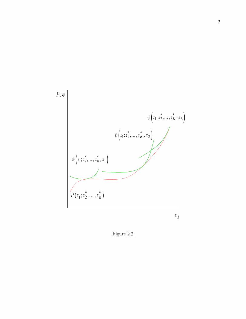
2
* *1 2( ; , , )KP z z z
,P
* *1 2 3; , , ,Kz z z
1 2* *
1; , , ,Kz z z
* *1 2 2; , , ,Kz z z
1z
Figure 2.2:

3
, ,P
z
12
3
1 2
3
P
Figure 2.3:
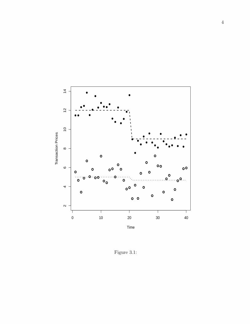
4
●
●
●
●
●
●
●
● ●
●
●●
● ●
●
●
●
●
●●
●
●
●
●
●
●
●
●
●
● ●
●
●
●
●
●
●●
● ●
0 10 20 30 40
24
68
10
12
14
Time
Tra
nsa
ctio
n P
rice
s
● ●
●●
●
●
●
●
●
●
● ●●
●
●
●
●
●
●
●
●
●
●
●
●
●
●
●●
●
●
●●
●●
●
●
●
●
●
Figure 3.1:
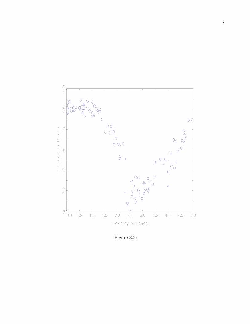
5
Figure 3.2:
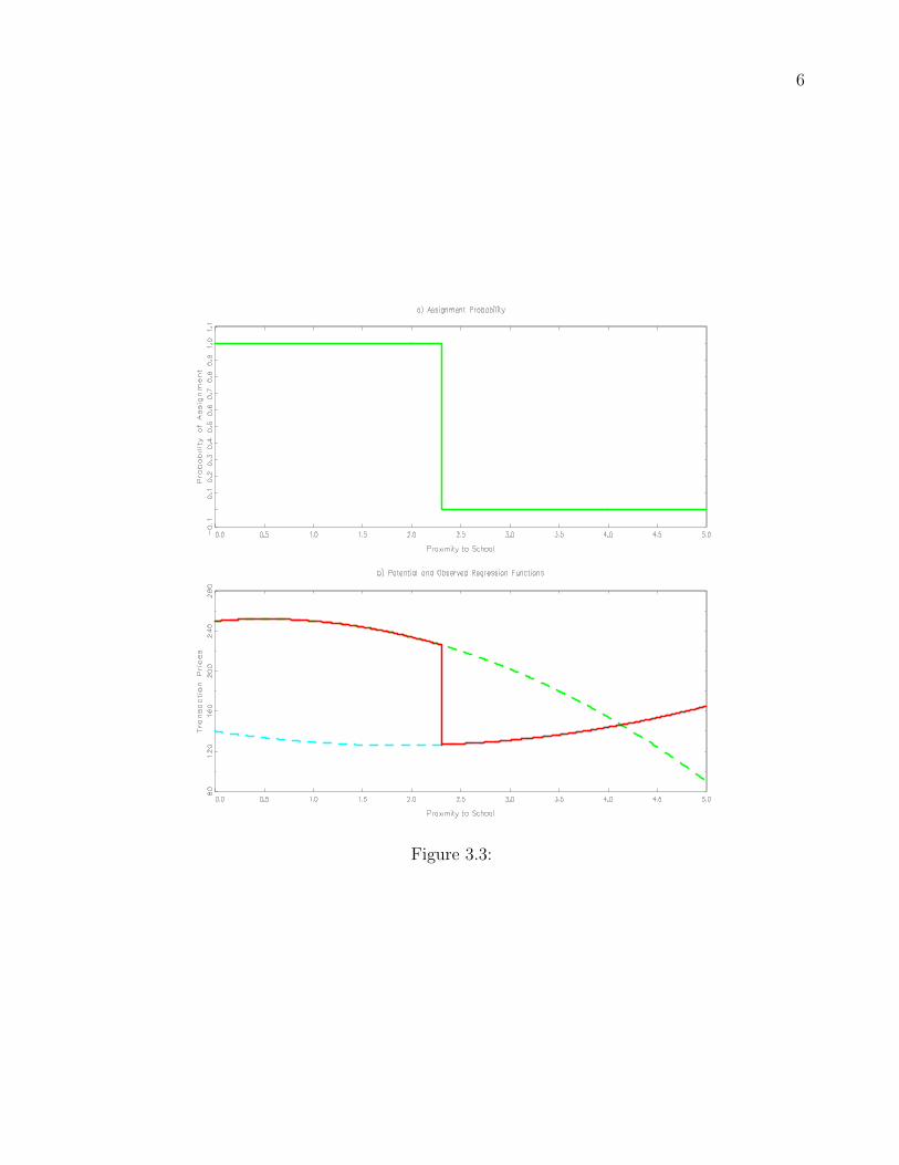
6
Figure 3.3:
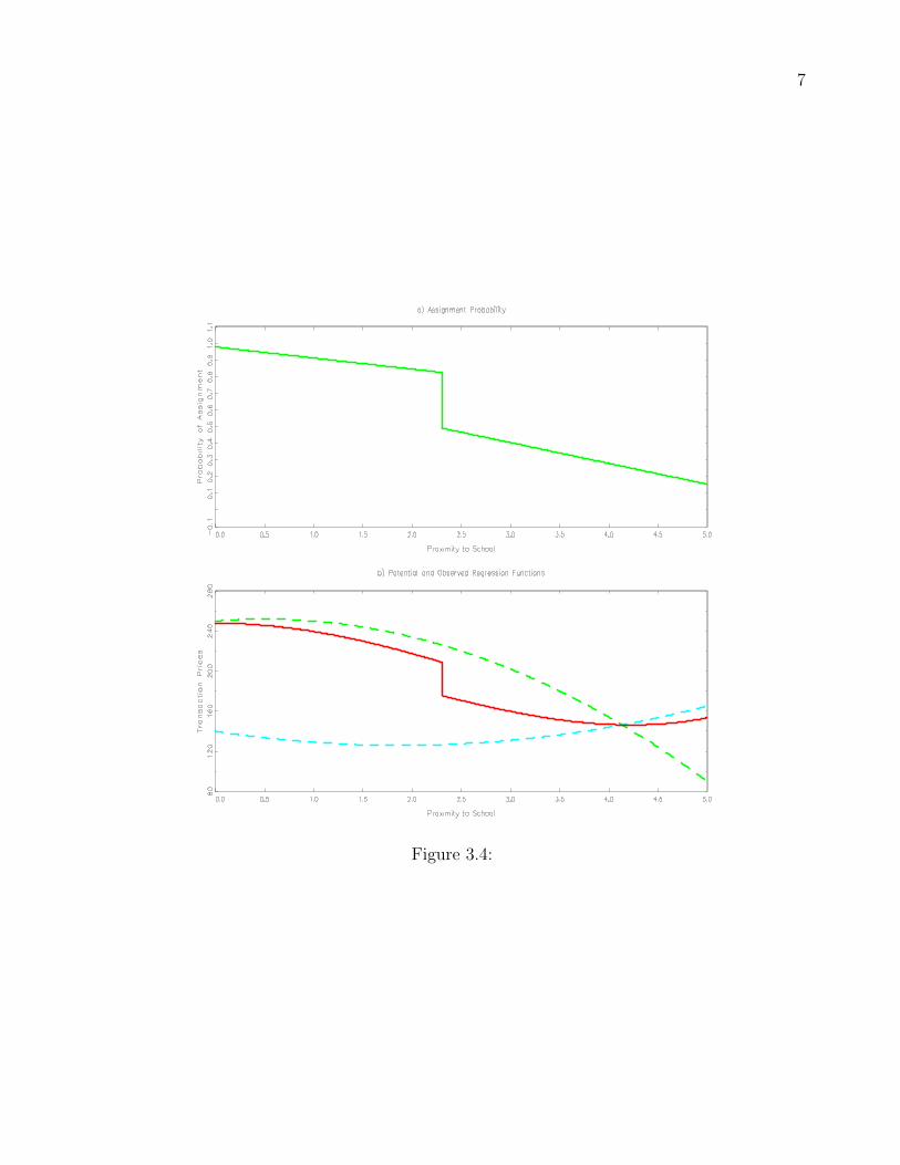
7
Figure 3.4:
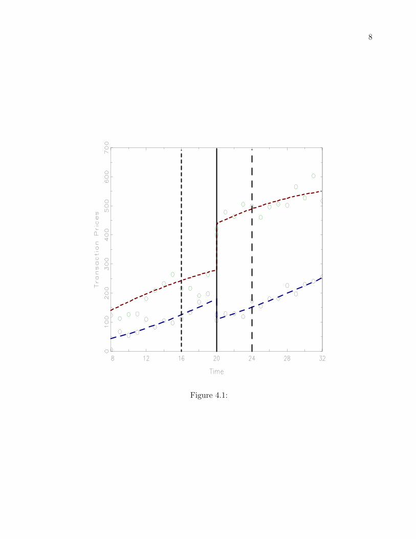
8
Figure 4.1:
9
Figure 5.1:

10
Figure 5.2:
11
Figure 5.3:


