Download - Quantitative Stock Selection
Quantitative Stock Selection
James F. Page III, CFA
May 2005
Project Summary
1. Why Quant Selection is Attractive
2. Methodology
3. Historical Back Testing
4. Model Results
5. Dynamic Weights / Regime Change
6. Benchmarks
7. Next Generation Models
8. Concluding Thoughts

I. Quantitative Stock Selection

Quant Stock Selection
Premise
(1) In aggregate, certain fundamental, expectational, and macro variables may contain valuable information in predicting stock returns
(2) Not unlike traditional fundamental analysis, just more systematic
Quant Stock SelectionPros: Anecdotal evidence suggests ~80% of stock picking is done ‘by
hand’ (individuals making calls on fundamentals) Relies heavily on talent (or luck) of individual analyst Individuals can only process so much information (sector focus) Human nature suggests cognitive biases likely
Market structure may perpetuate mis-pricings (Street incentives, value weighted benchmarks, short sale restrictions)
Little academic research on subject (trade rather than publish) Evidence suggests that investors systematically over pay for
‘growth’ Quantitative selection is scaleable
Quant Stock SelectionCons: Black box nature of model
Explain approach without revealing too much information Attribution analysis – must be able to explain performance
Protecting against common modeling errors Credibility of simulated results Adapting to individual client restraints
Quant Stock Selection
Market Neutral
Generate returns from both undervalued and overvalued stocks At present, high market valuation = low future returns Market exposure is commodity but good stock selection is valued
(higher management fees) Low return expectations combined with geo-political environment
suggests absolute return approach prudent

II. Methodology
Methodology
1. Hypothesize Develop candidate list of potential factors that may assist in
predicting stock returns (valuation, growth, etc.) ‘Priors’ reduce data mining
2. Back Test Decide on “universe” for testing (capitalization, index, sector, etc) Use sorting or regressions to test individual candidate variables FactSet’s AlphaTester currently available to Duke students
3. Rebalance Periodically rebalance portfolios (monthly, annually, etc.)
Methodology
4. Analyze Results Consider factor performance and consistency (both long and
short candidates) in predicting returns balanced against turnover
Select most promising factors for inclusion in the model
5. Weight Once individual factors selected must decide on weights for
final model by either:a) ‘Eye balling’ best factors and assigning weights for a scoring
model
b) Pushing individual factor portfolios into a mean-variance optimizer

III. Historical Back Testing
Historical Back Testing
Access to reasonably accurate historical data is costly FactSet’s AlphaTester is currently available to Duke students Two approaches common in practice
Regression of factors on security returns (Panel, etc.) Sorting universe into fractiles based on factor characteristics (AlphaTester)
Must protect against common modeling errors Survivorship bias Information / reporting lags Data mining Inaccuracies in data
Credibility of simulated returns is critical
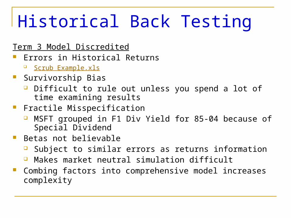
Historical Back TestingTerm 3 Model Discredited Errors in Historical Returns
Scrub Example.xls Survivorship Bias
Difficult to rule out unless you spend a lot of time examining results Fractile Misspecification
MSFT grouped in F1 Div Yield for 85-04 because of Special Dividend
Betas not believable Subject to similar errors as returns information Makes market neutral simulation difficult
Combing factors into comprehensive model increases complexity
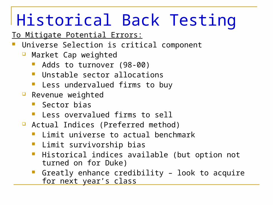
Historical Back TestingTo Mitigate Potential Errors: Universe Selection is critical component
Market Cap weighted Adds to turnover (98-00) Unstable sector allocations Less undervalued firms to buy
Revenue weighted Sector bias Less overvalued firms to sell
Actual Indices (Preferred method) Limit universe to actual benchmark Limit survivorship bias Historical indices available (but option not turned on for Duke) Greatly enhance credibility – look to acquire for next year’s
class

Historical Back TestingTo Mitigate Potential Errors: Factor Syntax
If you do not get this right – data is worthless (lots of opportunities to get it wrong)
Consider consolidating our “approved” syntax for future students as starting point
Expectational (instead of accounting/fundamental) produced significantly fewer errors
Survivorship Bias Selecting “Research Companies” does not protect without:
Appropriate Syntax on Factors Correct specification of Universe
Sanity checks on early period companies # of NA companies can be signal
Errors You must clean historical data Consider median returns as back of envelope option
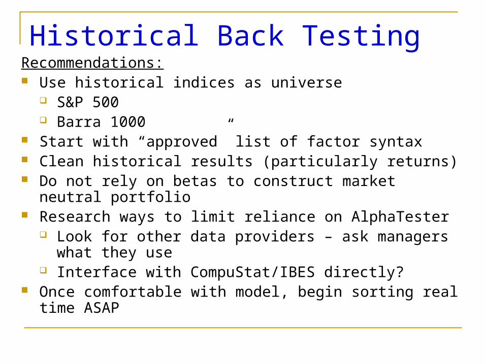
Historical Back TestingRecommendations: Use historical indices as universe
S&P 500 Barra 1000
Start with “approved” list of factor syntax Clean historical results (particularly returns) Do not rely on betas to construct market neutral portfolio Research ways to limit reliance on AlphaTester
Look for other data providers – ask managers what they use Interface with CompuStat/IBES directly?
Once comfortable with model, begin sorting real time ASAP

IV. Model Results

Model Results
Desired Universe: S&P 500
Why: ‘Considered’ to be highly efficient Value weighted index suggests low hanging fruit Historical data for testing is plentiful and reasonably accurate Highly liquid (market impact costs and borrow) Very scaleable because of market capitalizations
Actual Universe: First choose US Companies with highest sales (~ 500) Had to switch to Market Cap because of data limitations
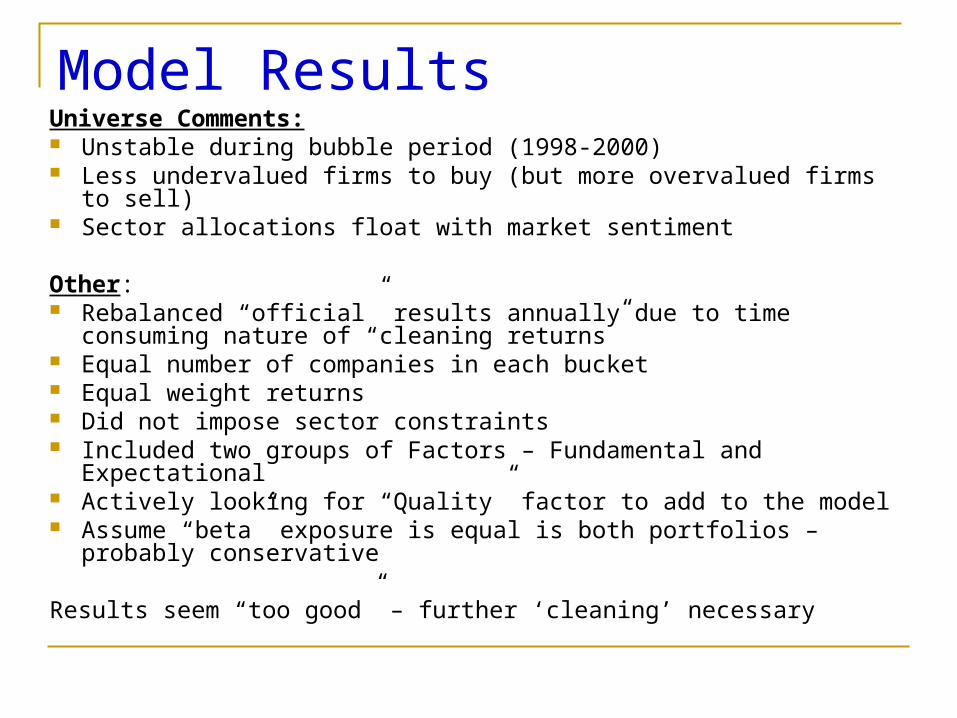
Model ResultsUniverse Comments: Unstable during bubble period (1998-2000) Less undervalued firms to buy (but more overvalued firms to sell) Sector allocations float with market sentiment
Other: Rebalanced “official” results annually due to time consuming nature
of “cleaning returns” Equal number of companies in each bucket Equal weight returns Did not impose sector constraints Included two groups of Factors – Fundamental and Expectational Actively looking for “Quality” factor to add to the model Assume “beta” exposure is equal is both portfolios – probably
conservative
Results seem “too good” – further ‘cleaning’ necessary

Model ResultsIndividual Factor Performance
Monthly Statistics 1989 – 2004
Long Factors correlated with Value and visa versa
View Portfolios
Date F1 F2 E1 E2 F1 F2 E1 E2Mean 1.31% 1.14% 1.47% 1.47% 1.09% 0.95% 0.85% 0.77%Median 1.65% 1.13% 1.76% 1.87% 1.29% 1.08% 1.26% 1.34%High 20.50% 11.78% 14.15% 13.84% 27.40% 16.35% 28.57% 23.83%Low -14.59% -12.73% -15.00% -19.03% -19.64% -17.20% -25.75% -19.91%St Dev 4.87% 3.74% 4.96% 5.40% 6.30% 5.30% 7.35% 5.74%
CorrelationsS&P 500 82% 81% 83% 89% 75% 85% 73% 75%500 / Growth 70% 66% 69% 78% 81% 85% 78% 78%500 / Value 89% 89% 91% 93% 59% 75% 60% 63%
Long Factors Short Factors
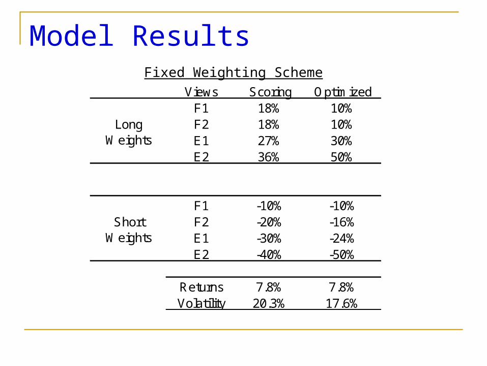
Model ResultsFixed Weighting Scheme
Views Scoring OptimizedF1 18% 10%F2 18% 10%E1 27% 30%E2 36% 50%
F1 -10% -10%F2 -20% -16%E1 -30% -24%E2 -40% -50%
Returns 7.8% 7.8%Volatility 20.3% 17.6%
Long Weights
Short Weights
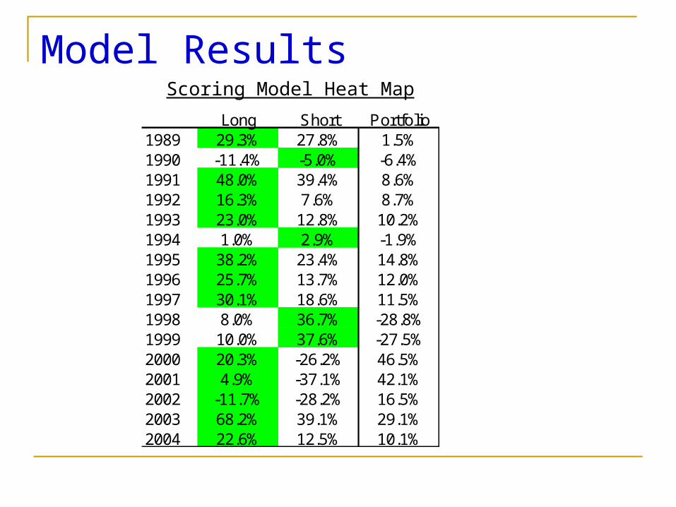
Model ResultsScoring Model Heat Map
Long Short Portfolio1989 29.3% 27.8% 1.5%1990 -11.4% -5.0% -6.4%1991 48.0% 39.4% 8.6%1992 16.3% 7.6% 8.7%1993 23.0% 12.8% 10.2%1994 1.0% 2.9% -1.9%1995 38.2% 23.4% 14.8%1996 25.7% 13.7% 12.0%1997 30.1% 18.6% 11.5%1998 8.0% 36.7% -28.8%1999 10.0% 37.6% -27.5%2000 20.3% -26.2% 46.5%2001 4.9% -37.1% 42.1%2002 -11.7% -28.2% 16.5%2003 68.2% 39.1% 29.1%2004 22.6% 12.5% 10.1%
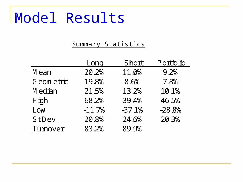
Model Results
Summary Statistics
Long Short PortfolioMean 20.2% 11.0% 9.2%Geometric 19.8% 8.6% 7.8%Median 21.5% 13.2% 10.1%High 68.2% 39.4% 46.5%Low -11.7% -37.1% -28.8%St Dev 20.8% 24.6% 20.3%Turnover 83.2% 89.9%

V. Dynamic Weights / Regime Change
Dynamic Weights / Regime Change A factor’s effectiveness may vary in different states of
nature (PE ratios impacted by inflation) Certain market / macro conditions may favor growth or
value (value was dog in late 1990s) Dynamic factor weights allow model to capitalize on
conditional information Few managers currently employ dynamic weighting
schemes This area “is the Holy Grail” of Quant Strategies
Dynamic Weights / Regime ChangeForecasting Regime Change Inflection point for style (growth or value) relative performance Used S&P 500 Barra Value and Growth Indices as Proxies Examined macro economic variables that might assist in
forecasting these inflection points Two variables demonstrated “promise” in forecasting style relative
performances over the following year
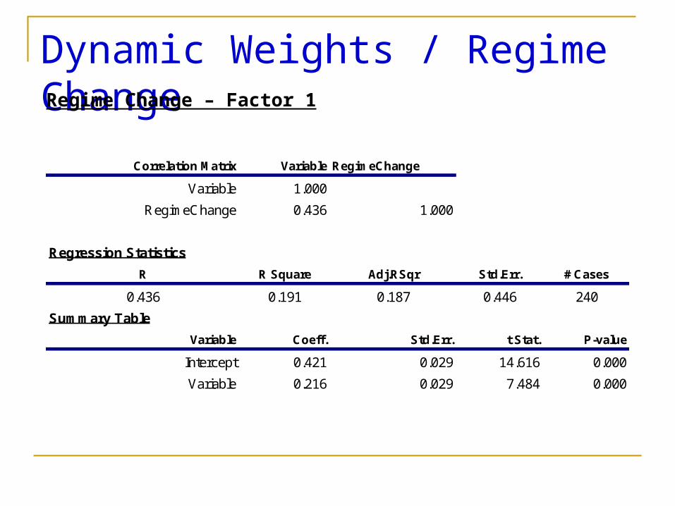
Dynamic Weights / Regime ChangeRegime Change – Factor 1
Correlation Matrix Variable RegimeChange
Variable 1.000
RegimeChange 0.436 1.000
Regression Statistics
R R Square Adj.RSqr Std.Err. # Cases
0.436 0.191 0.187 0.446 240
Summary Table
Variable Coeff. Std.Err. t Stat. P-value
Intercept 0.421 0.029 14.616 0.000
Variable 0.216 0.029 7.484 0.000

Dynamic Weights / Regime ChangeRegime Change – Factor 2
Correlation Matrix RegimeChange Variable
RegimeChange 1.000
Variable 0.411 1.000
Regression Statistics
R R Square Adj.RSqr Std.Err. # Cases
0.411 0.169 0.165 0.452 240
Summary Table
Variable Coeff. Std.Err. t Stat. P-value
Intercept 0.421 0.029 14.424 0.000
Variable 0.203 0.029 6.952 0.000

Dynamic Weights / Regime ChangeThe Same Can Be Applied to View Portfolios
Expectational Factor #2 and Regime Change Factor #1:Prediction of Long outperforming Short
Correlation Matrix Variable E2 Long / Short
Variable 1.000
E2 Long / Short 0.435 1.000
Regression Statistics
R R Square Adj.RSqr Std.Err. # Cases
0.435 0.189 0.184 0.388 169
Summary Table
Variable Coeff. Std.Err. t Stat. P-value
Intercept 0.776 0.030 25.848 0.000
Variable 0.176 0.028 6.240 0.000

Dynamic Weights / Regime ChangeThe Same Can Be Applied to View Portfolios
Expectational Factor #2 and Regime Change Factor #2:Prediction of Long Outperforming Short
Correlation Matrix E2 Long / Short Variable
E2 Long / Short 1.000
Variable 0.427 1.000
Regression Statistics
R R Square Adj.RSqr Std.Err. # Cases
0.427 0.183 0.178 0.390 169
Summary Table
Variable Coeff. Std.Err. t Stat. P-value
Intercept 0.788 0.030 25.922 0.000
Variable 0.171 0.028 6.110 0.000

VI. Benchmarks
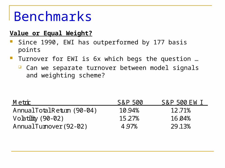
BenchmarksValue or Equal Weight? Since 1990, EWI has outperformed by 177 basis points Turnover for EWI is 6x which begs the question …
Can we separate turnover between model signals and weighting scheme?
Metric S&P 500 S&P 500 EWIAnnual Total Return ('90-'04) 10.94% 12.71%Volatility ('90-'02) 15.27% 16.04%Annual Turnover ('92-'02) 4.97% 29.13%
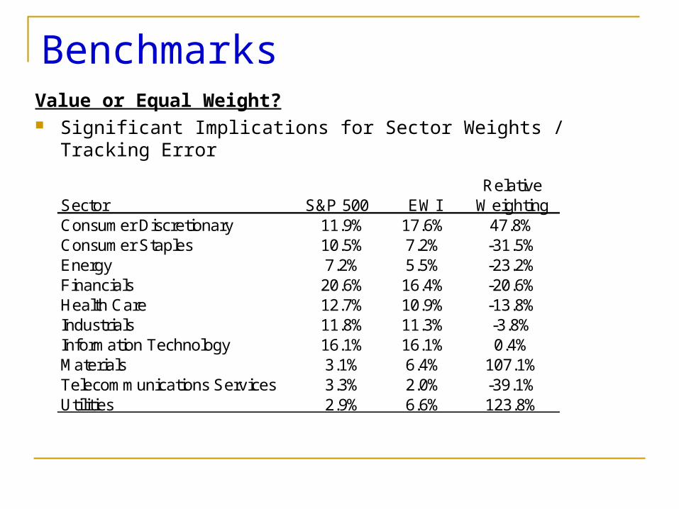
BenchmarksValue or Equal Weight? Significant Implications for Sector Weights / Tracking Error
RelativeSector S&P 500 EWI WeightingConsumer Discretionary 11.9% 17.6% 47.8%Consumer Staples 10.5% 7.2% -31.5%Energy 7.2% 5.5% -23.2%Financials 20.6% 16.4% -20.6%Health Care 12.7% 10.9% -13.8%Industrials 11.8% 11.3% -3.8%Information Technology 16.1% 16.1% 0.4%Materials 3.1% 6.4% 107.1%Telecommunications Services 3.3% 2.0% -39.1%Utilities 2.9% 6.6% 123.8%
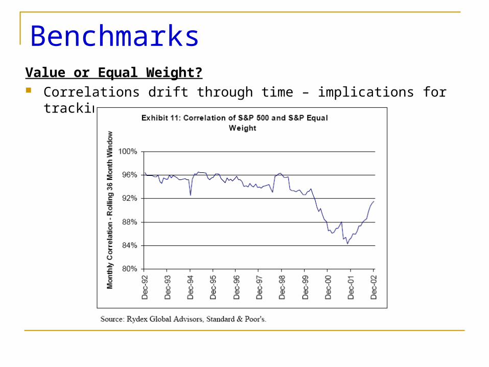
BenchmarksValue or Equal Weight? Correlations drift through time – implications for tracking error

BenchmarksValue or Equal Weight? EWI had positive loading on the size premium EWI has significant exposure to the value premium
Fama-French Risk Factor Exposures
500 EWIIntercept 0.413 0.385Market 1.009 1.060SMB Premium (0.181) 0.060HML Premium 0.050 0.370R-squared 99% 93%
Source: http://mba.tuck.dartmouth.edu/pages/faculty/ken.french/data_library.html

BenchmarksValue or Equal Weight? EWI has 82% correlation with 500 / Barra Growth EWI has 96% correlation with 500 / Barra Value Further proof of value tilt
500 / 500 /500 EWI Barra Growth Barra Value
500 100%EWI 93% 100%500 / Barra Growth 96% 82% 100%500 / Barra Value 94% 96% 81% 100%

BenchmarksValue or Equal Weight? Obvious Pros and Cons to both EWI benchmark will make returns look less impressive, but
help explain turnover EWI may be a better match for style Provide more stable weighting for sector allocations Equal weight is newer idea – historical data is limited If possible, choice should match weighting scheme of
portfolio

VII. Next Generation Models

Next Generation Models Refining Dynamic Factor Weights
Preferably done outside of FactSet Migration Tracking
May contain information to enhance returns or limit turnover
♥ ♥ ♥ ♥ ♥ ♥ ♥♣
♥ ♥ ♥♣ ♣
♣ ♣
♣ ♣ ♣
♣ ♣1 2 3 4 5 6 7 8 9 10
Fractile 5
Periods
♥ Score of Stock X ♣ Score of Stock Y
Fractile 1
Fractile 2
Fractile 3
Fractile 4

Next Generation ModelsModified Versions of S&P 500 Model Separate Models for Sector and Stock Selection More Conservative
More positions Limited tracking error
More Aggressive Directional Less positions Leverage
Other Domestic Models S&P Mid-Cap 400 / Russell 2000
International Models Developed / Emerging markets

VIII. Concluding Thoughts

Concluding ThoughtsTheoretical How long will excess returns exist How to stay ‘ahead of the curve’
Implementation Cost of data Credibility of simulation Returns during first 12 – 24 months Balance between turnover and model signals
Concluding Thoughts
Overall Quantitative Stock Selection Appealing Outperformance Seems Possible Long/Short Consistent with Absolute Return Approach

Bio
James F. Page III
Jimmy became interested in quantitative stock selection during Campbell Harvey’s Global Asset Allocation and Stock Selection class and a follow-up course dedicated to quantitative stock selection. He received his Bachelor of Science degree from the University of Florida and will receive his MBA from Duke University’s Fuqua School of Business in May 2005. Prior to enrolling at Duke, he spent four years in the Equity Research Department of Raymond James & Associates in St. Petersburg, FL. He is also a CFA charter holder.


