
1
Pseudo Panel Data Estimation Technique and Rational Addiction Model:
An Analysis of Tobacco, Alcohol and Coffee Demands
Aycan Koksal Cleveland State University
Department of Economics
Michael Wohlgenant
North Carolina State University
Department of Agricultural and Resource Economics [email protected]
Selected Paper prepared for presentation at the Agricultural & Applied Economics
Association’s 2013 AAEA & CAES Joint Annual Meeting, Washington, DC, August 4-6, 2013
Preliminary Draft - Please do not cite
Copyright 2013 by Aycan Koksal and Michael Wohlgenant. All rights reserved. Readers may
make verbatim copies of this document for non-commercial purposes by any means, provided that
this copyright notice appears on all such copies.

2
In this paper, we generalize the rational addiction model to include three
addictive goods: cigarettes, alcohol and coffee. We use a pseudo-panel data
approach which has many advantages compared to aggregate and panel data. While
cigarette and coffee demands fit well with the rational addiction model, alcohol
demand does not. This result might be due to possible inventory effects. Our results
suggest that although cigarettes and alcohol reinforce each other in consumption,
consumers substitute them when there are permanent changes in relative prices. In
the semi-reduced system, the cross-price elasticity of coffee demand with respect to
cigarette price is positive and significant. Long-run cross-price elasticities derived
from the semi-reduced system and the Morishima elasticities show that when relative
prices increase, consumers substitute addictive goods with other addictive goods.
This is likely due to compensation and income effects. When there is a permanent
increase in relative prices, addicts cut the consumption of a harmful addictive
substance, and substitute it with another addictive substance to compensate for the
resulting stress. Moreover, when the consumption of an addictive substance
decreases after a price increase, relative consumption of other substances increase
due to the positive income effect.
Key words: cigarette, alcohol, coffee, rational addiction, pseudo panel
3
The rational addiction model (Becker and Murphy, 1988) is the most popular framework used to
estimate the demand for addictive goods. In myopic demand models of addictive behavior, past
consumption increases current consumption, but consumers do not take into account the future
consequences of their actions when they make current consumption decisions. In the rational
addiction model, the consumer is aware of the future consequences of addiction and accounts for
them when making consumption choices. In the rational addiction model, both past and
anticipated future consumption affect current consumption positively.
Bask and Melkersson (2004) extended the rational addiction model to allow for commodity
addictions in two addictive goods: alcohol and cigarettes. This paper extends their model by
analyzing the interdependence among three addictive goods in a rational addiction framework:
cigarettes, alcohol and coffee.
The rational addiction model has been previously applied to cigarette consumption (e.g.,
Becker et al., 1994), alcohol consumption (e.g., Grossman et al., 1998) and coffee consumption
(e.g., Olekalns and Bardsley, 1996), separately. Many papers claim interdependence between
cigarette and alcohol consumption using the myopic or rational addiction models. On the other
hand, to the best of our knowledge, there is no paper that analyzes the relationship between the
consumption of coffee and other addictive goods like cigarettes and alcohol using a theoretical
framework.
Zavela et al. (1990) examined the relation between cigarettes, alcohol, and coffee
consumption among army personnel. They found that, for women, cigarette and alcohol
consumption are positively correlated; but, for men, cigarette and coffee consumption are
4
positively correlated. In addition, they found a pattern of abstention from alcohol and coffee
among nonsmokers.
In this paper, we analyze the relationship between cigarettes, alcohol and coffee consumption
in a rational addiction framework using a pseudo-panel data approach. The objectives of this
study are twofold: First, to gain more insight into behavioral processes concerning cigarettes,
alcohol and coffee consumption; second, to generalize the rational addiction model to include
three addictive goods to provide a framework for future research in the related literature (e.g.,
interdependence among cigarettes, alcohol and marijuana or interdependence among cigarettes
and different types of alcoholic beverages such as beer and wine).
Theoretical Model
Following Bask and Melkersson (2004), we assume:
where , and are the quantities of cigarettes, alcohol and coffee consumed; , and
are the habit stocks of cigarettes, alcohol and coffee respectively; is the consumption of a
non-addictive composite good.
We assume a strictly concave utility function. The marginal utility derived from each good is
assumed to be positive ( i.e., , and ; concavity implies ,
and ). Following the rational addiction literature, we assume that
habit stocks of cigarettes and alcohol affect current utility negatively due to their adverse health
effects ( i.e., < 0 and ; concavity implies and ). Since coffee use is

5
not associated with adverse health effects, we don’t impose any assumptions on the marginal
utility of habit stocks of coffee.
Reinforcement implies , . Cigarette, alcohol and coffee
consumption are assumed to have no effect on the marginal utility derived from the consumption
of the composite good (i.e., ).
If alcohol (cigarette) consumption decreases the marginal utility derived from cigarette
(alcohol) consumption, < 0 and < 0; if alcohol consumption reinforces cigarette
consumption and vice versa, and .
If past alcohol consumption increases the marginal utility from current cigarette consumption,
; if past cigarette consumption increases the marginal utility from current alcohol
consumption, . Pierani and Tiezzi (2009) name this intertemporal cross-reinforcement
effect the quasi-gateway effect.1 When cigarette consumption does not affect the marginal utility
from alcohol consumption and vice versa
If coffee consumption reinforces cigarette consumption, > 0 and > 0; and if coffee
consumption decreases the marginal utility from alcohol consumption, < 0 and < 0. When
consumption of coffee does not affect the marginal utility from cigarette consumption,
. When consumption of coffee does not affect the marginal utility from
alcohol consumption, .
1 A true gateway effect refers to the condition that consumption of one addictive substance leads to later initiation of
another addictive substance (Pacula,1997).

6
The intertemporal budget constraint is
where with r being the discount rate, , and are prices of cigarettes,
alcohol and coffee, respectively, and is the present value of wealth. The composite good, N, is
taken as the numeraire good.
Then the consumer’s problem is:
As in previous studies, we assume that and When the
utility function is quadratic, the solution to problem (3) generates the following demand
equations2:
2 See Appendix A for derivation of Equations (4)-(6).

7
As pointed out by Bask and Melkersson (2004), the rational addiction model nests many
different behaviors: “A non-addicted consumer responds only to information in the current period,
which means that the parameters for those variables which correspond to the past and the future
are zero. An addicted but myopic consumer also responds to past information. Finally, an
addicted consumer who is also rational responds to past, current, and future information” (p.375).
The specification also allows for quasi-gateway effects across different addictive goods. The
nested structure is convenient for testing certain parameter restrictions to evaluate the merits of a
generalization.
In the empirical model, in addition to the variables that directly come from the theoretical
model, for each equation we add an error term , some consumer demographics ( and an
individual fixed effect ( to account for unobserved individual heterogeneity, such as attitudes
towards health risks.
For k=1,2,3 economic theory implies Rational addiction implies
with From the structural parameters, the rate of time preference can be derived
for each good3. In the applied literature, these parametric restrictions have been tested to check
the validity of the rational addiction model.
For k=1,2, if smoking and drinking reinforce each other; and if drinking
makes it easier to abstain from smoking, and vice versa. If alcohol consumption is a
quasi-gateway for cigarette consumption, if cigarette consumption is a quasi-gateway for
alcohol consumption.
3 In empirical applications it is possible to find different rate of time preference, r, for different addictive goods.
8
If then coffee and cigarette consumption reinforce each other. If then coffee
consumption makes it easier to abstain from alcohol consumption.
Data
Consumer Expenditure Survey(CEX) Diary data by Bureau of Labor Statistics(BLS) are used in
this study. Cigarette, alcohol and coffee expenditures, together with price variables, are used to
calculate (average weekly) consumptions (i.e., cigarette consumption= cigarette expenditure/
cigarette price).
The observations with missing state variables are dropped. To avoid any inconsistency, we
also dropped the very few households that report different household head demographics (i.e.,
race, education) for each week that the Diary data are collected.
Because price data are not collected by CEX, price variables used in the analysis are gathered
from other data sources. All price variables are deflated by the CPI for all items reported on the
BLS webpage. Annual state level cigarette prices are gathered from the website of Department of
Health and Human Services, Centers for Disease Control and Prevention (CDC). To obtain
alcoholic beverages prices, we construct Lewbel (1989) price indices that have household specific
price variation4. Regional coffee prices reported monthly on the BLS webpage are used to obtain
quarterly coffee prices5.
4 See Appendix B for derivation of Lewbel price indices.
5 Regional coffee prices are not reported for the most recent years, we derived those using monthly coffee price index
and the previous month’s coffee price.
9
Methodology
Although individual level panel data have many advantages compared to aggregate data, they
generally span short time periods, suffer from measurement error and are subject to attrition bias.
In order to avoid these problems, Deaton (1985) suggested using pseudo-panel data approach as
an alternative method for estimating individual behavior models.
In the literature, for estimating dynamic models of demand, the pseudo-panel method is a
relatively new econometric method. It is an instrumental variables approach in which cohort
dummies are used as instruments in the first-stage (i.e., the first stage predicted values are
equivalent to cohort averages). The pseudo-panel approach enables one to follow cohorts of
people through repeated cross-sectional surveys. Because repeated cross-sectional surveys are
often over longer time-periods than true panels, with pseudo panel method models can be
estimated over longer time periods. Moreover, averaging within cohorts removes individual-level
measurement error (see Antman and McKenzie, 2007).
In pseudo-panel analysis, because cohorts are followed over time, they are constructed based
on characteristics that are time invariant, such as geographic region or the birth year of the
reference person. When we construct cohorts, we face a trade-off between the number of cohorts
and the number of individuals within cohorts. If individuals are allocated into a large number of
cohorts, there will be few observations in the cohorts which might cause biased estimators. On the
other hand, if only a few cohorts are chosen to have a large number of observations per cohort,
individuals within a cohort might be heterogeneous, which would cause inefficiency. Thus, the
challenge when we construct a pseudo-panel is finding a balance between the number of cohorts
and the number of individuals within cohorts. The optimal choice would be the one that

10
minimizes the heterogeneity within each cohort but maximizes the heterogeneity among them. In
that case, pseudo-panel method results in consistent and efficient estimators.
In most of the applied pseudo-panel studies, the sample is divided into a small number of
cohorts with a large number of observations in each (e.g., Browning et al., 1985; Blundell,
Browning and Meghir 1994; Propper, Rees and Green 2001). Verbeek and Nijman (1992) showed
that if cohorts contain at least 100 individuals and there is sufficient time variation in the cohort
means, the bias due to measurement error would be small and can be ignored6.
In the pseudo-panel approach, cohorts can be constructed based on a single characteristic (i.e.,
birth cohort) or multiple characteristics (i.e., birth and region; birth and education, birth and
gender, etc). In this study, we form pseudo-panels based on household head’s year of birth and the
geographic region. Cohorts are defined by the interaction of three generations (born before 1950,
born between 1950-1964, born in 1965 or later) and four geographic regions (northeast, midwest,
south, west). For example, all household heads born before 1950 that reside in the northeast
would form one cohort and all households born before 1950 that reside in the midwest would
form another cohort. The resulting pseudo-panel consists of a total of 336 observations over 12
cohorts and 28 quarters. This allocation results in around 100 households per cohort.
Because pseudo-panel approach is an instrumental variables (IV) method, standard IV
conditions should be satisfied for identification (Verbeek and Vella, 2005). The time-invariant
instruments should have correlation not only with the lagged and lead consumption variables but
also with the exogenous variables in the model (i.e., sufficient cohort-specific variation should be
present in the exogenous variables). When we construct our cohorts, we take into account
6 They also state that the cohort sizes may be smaller than 100 observations if the individuals grouped in each cohort
are sufficiently homogeneous.
11
standard instrumental variables (IV) conditions. To have (time-variant) correlation between the
model variables and the time invariant instruments (i.e., cohort dummies), we construct our
cohorts based on household head’s year of birth and the geographic region. The three generations
(born before 1950, born between 1950-1964, born in 1965 or later) are likely to have different
consumption patterns which are subject to change over time as the generations age. Different
generations are likely to differ also in terms of consumer demographics (e.g., preference for small
versus large families) which can change as generations age (e.g., family size changes as children
leave the house to start their own family). There are also differences across regions in terms of
prices, consumer demographics, and consumption patterns which would change over time
because of migration, local policy changes, etc.
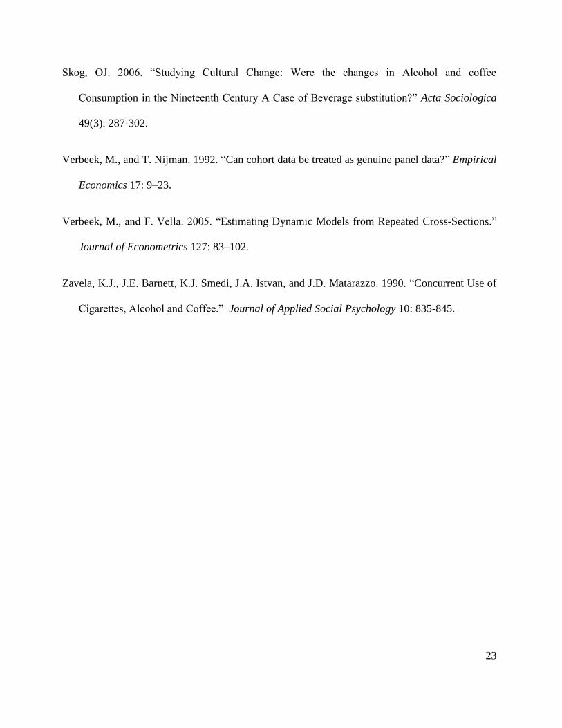
Figure 1 shows cigarette consumption by birth cohorts over the sample period. The youngest
birth cohort has an increasing cigarette consumption on average, while the average cigarette
consumption of older cohorts are decreasing from 2002 to 2008. The oldest cohort (i.e., people
born before 1950) has the lowest cigarette consumption. Their low (and decreasing) consumption
can be attributed to age related health problems which force older consumers to cut back cigarette
consumption. The highest cigarette consumption is observed among the people born between
1950-1964, which slightly decreases over the sample period. The people born after 1964 have a
lower cigarette consumption compared to people born in 1950-1964. This can be explained by the
1964 surgeon general’s report on smoking. The 1964 surgeon general’s report caused awareness
about the health consequences of smoking and changed public attitudes towards smoking.
12
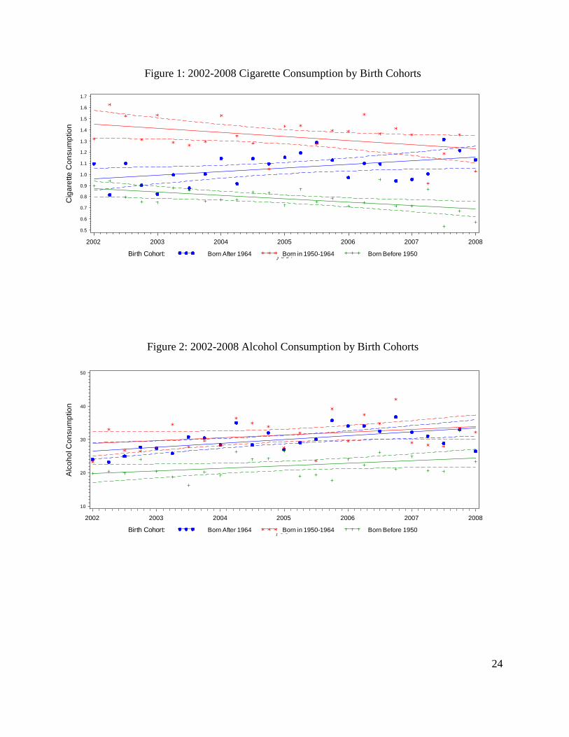
Figure 2 shows alcohol consumption by birth cohorts over the sample period. From 2002 to
2008, the average alcohol consumption slightly increases for all birth cohorts. The oldest birth
cohort (i.e., born before 1950) has the lowest alcohol consumption on average.
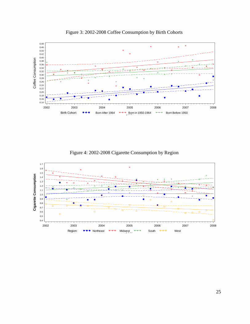
Figure 3 shows coffee consumption by birth cohorts over the sample period. From 2002 to
2008, the average coffee consumption increases for all birth cohorts. The youngest birth cohort
(i.e., born after 1964) has the lowest coffee consumption on average.
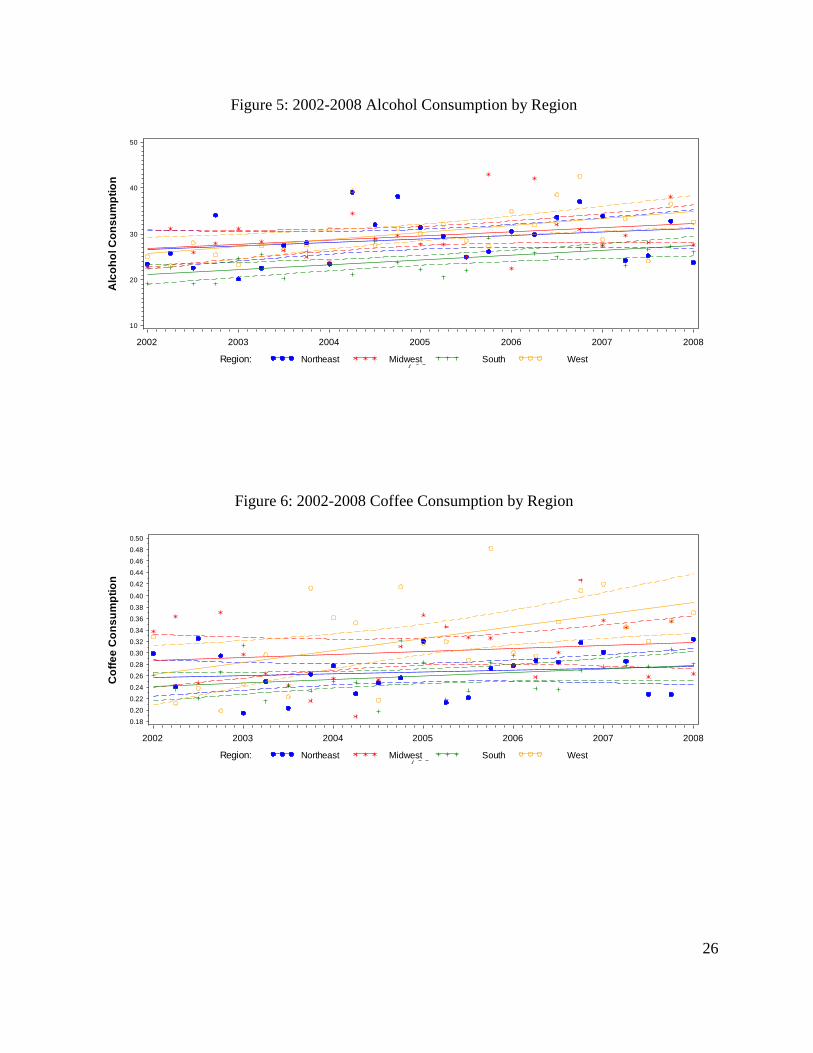
Figure 4, Figure 5 and Figure 6 show average consumptions by region. The midwest has the
highest cigarette consumption, while west has the lowest. Cigarette consumption decreases in the
midwest and west, while it increases in the south and northeast. Over the sample period alcohol
consumption slightly increases across all regions, and among all regions the south has the lowest
alcohol consumption. Coffee consumption increases across all regions, and the most significant
increase in consumption is observed in the west.
In section 2, we derived the structural equations of the following form:
In order the estimate the individual level structural equations (4) - (6), we use cohort dummies
as instruments in the first-stage. Taking cohort averages of (4) - (6), over individuals observed
in cohort c at time t results in:
13
where is the average of the fixed effects for those individuals in cohort c at time t.
In repeated cross-sectional surveys, different individuals are observed at each time period.
Thus, the lagged and lead variables are not observed for the same individuals in cohort c at time t.
Therefore, following the previous literature, we replace these sample means of the unobserved
variables with the sample means of the individuals at time t−1, and t+1, respectively, which leads
to the following equations7:
7 As the number of individuals in each cohort becomes large, the measurement error introduced by the use of pseudo-
panel analysis, i.e. converges to zero (McKenzie,2004).

14
Because the sample is collected separately for different time periods, is not constant over
time. can be treated as unobserved cohort fixed effect ( ) if there is sufficient number of
observations per cohort (see Verbeek and Nijman, 1992). In that case we can estimate the
structural equations at the cohort level by using cohort dummies or cohort fixed effects. In the
dynamic pseudo-panel data model, the fixed effects estimator on cohort averages is consistent
when T is small and provided that there are no cohort and time effects in the individual
error terms once controlled by cohort fixed effects (McKenzie, 2004). The number of
observations in each cohort is sufficiently large in our sample to ensure consistency (i.e., around
100 observations). Thus the fixed effects estimator on cohort averages is used.
In the sample, the number of households in each cohort and time period is not the same which
might induce heteroskedasticity. Following Dargay (2007), to correct for heteroskedasticity, all
cohort variables are weighted by the square root of the number of households in each cohort. To
obtain consistent standard errors, bootstrapped standard errors are calculated (1000 replications).
15
Empirical Results
First, each equation in (10) - (12) is estimated as a separate equation. The results are shown in
Table 1. Both cigarette and coffee demands are consistent with rational addiction (i.e., lag and
lead consumption coefficients are positive and significant). In both equations the coefficient on
lag consumption is higher than the lead consumption coefficient, implying the rate of
intertemporal preference is positive. In alcohol demand, lag and lead consumptions have negative
coefficients. This result might be due to inventory effects. In the alcohol demand equation, current
cigarette consumption has a positive and significant coefficient suggesting that current cigarette
consumption reinforces current alcohol consumption. We have not found any proof of quasi-
gateway effects across cigarette and alcohol.consumptions.8 Lag alcohol (cigarette) consumption
in the cigarette (alcohol) demand equation is not significant. In coffee demand, the coefficients on
current cigarette and current alcohol consumptions are positive, but not statistically significant.
The implied discount rates, r, are derived from the parameter estimates of own lagged and
lead consumption ( ). They are positive and plausible for cigarette and coffee
consumption. It is 4.57% for cigarette consumption and 1.91% for coffee consumption. Because
cigarettes are more addictive than coffee, consumers of cigarettes are likely to be more myopic
than consumers of coffee.
Regarding demographics, as family size increases cigarette and alcohol consumptions
increase. Whites have a higher consumption of cigarettes and alcohol compared to other races.
8 Failure to find evidence for quasi-gateway effects does not mean that there are no true gateway effects. Our
results do not rule out the possibility that consumption of one substance leads to initiation of use of another
substance. Unfortunately, the way the model is formulated does not make it possible to test for these true gateway
effects.
16
The consumer units whose household head has at least an associate’s degree smoke less
cigarettes, but drink more alcohol and coffee compared to other consumer units. However the
effect of education on consumption is not statistically significant. Overall, consumer
demographics do not seem to affect coffee consumption significantly. On the other hand, cohort
fixed effects are jointly significant in all three equations. The p-value for the F-test is smaller than
1% suggesting one should account for unobserved cohort fixed effects (F-values are 7.02, 3.53
and 3.45 for cigarettes, alcohol and coffee, respectively).
Bask&Melkersson (2004) and Pierani&Tiezzi (2009) point out that decisions regarding
cigarette and alcohol consumptions are often made jointly. Thus following Bask and Melkersson
(2004), we combine equations (10) - (12) to estimate a semi-reduced system.
Because the parameters in these equations are non-linear functions of the parameters in
equations (10) - (12), we don’t have prior expectations for their signs. Instead, we focus on the
long-run demand elasticities.
The semi-reduced system is estimated by using iterated seemingly unrelated regression
(ITSUR) method. The model coefficients are reported on Table 3. The long-run price and income
17
elasticities calculated at the sample mean are shown on Table 4. The long-run own price
elasticities are negative for all three goods. Cigarette and coffee have inelastic demands while
alcohol demand is elastic. Bask and Melkersson (2004) also found that alcohol demand is elastic
in the long-run. An explanation for this might be that most alcoholic beverage drinkers are just
social drinkers. The income elasticity is positive and less than one for all three goods.
Regarding cross-price elasticities, only the cross-price elasticity of alcohol with respect to
cigarette price, and the cross-price elasticity of coffee with respect to cigarette price are
significant. The positive cross-price elasticities with respect to the cigarette price suggests that as
the cigarette price increases people compensate reduced cigarette consumption with increased
alcohol and coffee consumption.
Because the cross-price elasticity does not take into account the price sensitivity of the good
whose price has been changed, Morishima elasticities of substitution are also calculated for the
long-run. The elasticity of substitution measures how the relative consumption of two
goods changes along the indifference curve when the relative prices change. Morishima elasticity
of substitution is calculated using the formula:
(13)
where and
are Hicksian own and cross price elasticities.
Hicksian price elasticities are derived as
where is Marshallian cross-price
elasticity, is income elasticity and sj is budget share of good j.
Morishima elasticiticies of substitution point to significant compensating behavior. All the
Morishima elasticities of substitution are positive and significant. Except σAK, all the Morishima

18
elasticities of substitution are greater than one. This suggests that cigarette, alcohol and coffee
substitute each other along the indifference curve when the relative prices change. As the relative
price of alcohol increases, the share of both cigarette and coffee consumptions relative to alcohol
consumption increase suggesting that the consumer compensates reduced alcohol consumption
with other addictive goods. Similar compensating behaviors apply to coffee and cigarette
consumptions too.
Concluding Remarks
This study uses a pseudo-panel data approach to analyze the relationship between cigarettes,
alcohol and coffee consumption within the rational addiction framework. The specification that
we use is very general and nests several different behaviors and accounts for possible
relationships among the three addictive goods.
We found that cigarette and coffee consumptions are consistent with rational addiction
whereas alcohol consumption is not (i.e., in the alcohol demand equation lag and lead
consumptions have negative coefficients). If there are inventory effects, this might be the reason
why alcohol demand does not fit the theoretical model so well. In a different study (Koksal and
Wohlgenant, 2011) when we replaced “overall alcohol expenditures” with “restaurant alcohol
expenditures”, (restaurant) alcohol demand became consistent with rational addiction which
reinforces our belief that in the current study the inconsistency of alcohol demand with the
rational addiction model is due to inventory effects observed in quarterly alcohol expenditures.
The structural model does not suggest any significant reinforcement effect between coffee and
cigarette consumption. However this does not rule out the possibility that coffee and cigarette
19
consumption might reinforce each other for some subpopulations. On the other hand, in the semi-
reduced system, the cross-price elasticity of coffee demand with respect to cigarette price is
positive and significant suggesting that coffee substitutes for cigarettes when cigarette prices
increase.
Morishima elasticiticies of substitution point to significant compensating behavior (i.e.,
cigarette, alcohol and coffee substitute each other along the indifference curve when the relative
prices change). As the relative price of alcohol increases, the share of both cigarette and coffee
consumptions relative to alcohol consumption increase suggesting that the consumer compensates
reduced alcohol consumption with other addictive goods. Coffee and cigarette consumptions
provide similar compensating behaviors. When relative price of cigarettes (alcohol) increase,
consumers substitute cigarettes (alcohol) with alcohol (cigarettes). Our findings are consistent
with Picone et al.(2004) who claim that alcohol and cigarettes are gross substitutes in price
although they are complements in consumption for social drinkers. They explain positive cross-
price responses with compensation and income effects. When there is a permanent increase in
relative prices, addicts cut the consumption of a harmful addictive substance, and substitute it
with another addictive substance to compensate for the resulting stress. Moreover, when
consumption of an addictive substance decreases due to a price increase, consumption of other
addictive substances are likely to increase due to a positive income effect.
Although cigarette taxation has been cited as one of the most effective public health tools for
cigarette control, the empirical results suggest that increasing cigarette prices might increase
alcohol consumption (i.e., the cross-price elasticity of alcohol with respect to cigarette price is

20
positive and significant in the semi-reduced system). Because of compensating behaviors of
addicts, taxes might result in increases in the consumption of other addictive goods.
There are other studies that find evidence of addiction displacement. Using both qualitative
and quantitative data, Skog (2006) examines if the decline in the Norwegian alcohol consumption
during the nineteenth century is related to the growth of coffee culture as a substitute. He claims
that coffee filled a cultural ‘niche’ created by the restrictive Norwegian alcohol policy (i.e.,
decreased availability and increased taxes) in the nineteenth century. He concludes that the
decline in alcohol consumption was, in part, as a result of coffee substituting alcohol as an
alternative ‘new’ beverage for all social classes.
Reich et al. (2008) investigate coffee and cigarette use among recovering alcoholics that
participate in Alcoholics Anonymous (AA) meetings in 2007 in Nashville. They find that
cigarette and coffee consumption among AA members is higher compared to the general U.S.
population. Most recovering alcoholics explain that they consume coffee for its stimulatory
effects (i.e., feeling better, higher concentration, more alertness), and they consume cigarettes for
its reduction of negative feelings (i.e., depression, anxiety and irritability).
Many studies support that kicking a habit becomes much easier when addicts form a new
replacement habit. Our results suggest that if compensating behaviors can be channeled toward
harmless addictive substances such as caffeine or smokeless tobacco (e.g., Rodu and Cole, 2009
on smokeless tobacco consumption versus cigarette consumption), the unintended consequences
of increasing cigarette prices in the form of increased alcohol consumption can be avoided.
21
References
Bask, M., and M. Melkersson. 2004. “Rationally Addicted to Drinking and Smoking?” Applied
Economics 36:373-381.
Becker, G.S., K.M. Murphy.1988. “A Theory of Rational Addiction.” Journal of Political
Economy 96:675-700.
Becker, G.S., M. Grossman, and K.M. Murphy. 1994. “An Empirical Analysis of Cigarette
Addiction.”American Economic Review 84:396–418.
Dargay, J. 2007. “The effect of prices and income on car travel in the UK.” Transportation
Research Part A 41:949-960.
Deaton, A. 1985. “Panel data from time series of cross-sections.” Journal of Econometrics
30:109-126.
Grossman, M., F.J. Chaloupka, and I. Sirtalan. 1998 “An Empirical Analysis of Alcohol
Addiction: Results from the Monitoring the Future Panels.” Economic Inquiry 36:39–48.
Hoderlein, S., and S. Mihaleva. 2008. “Increasing the price variation in a repeated cross section.”
Journal of Econometrics 147:316-325.
Koksal A, Wohlgenant MK. (2011) How do Smoking Bans in Bars/Restaurants Affect Alcohol
Consumption? Agricultural and Applied Economics Association Annual Meeting, Pittsburgh,
Pennsylvania.

22
Lewbel, A. 1989. “Identification and estimation of equivalence scales under weak separability.”
Review of Economic Studies 56: 311-316.
McKenzie, D.J. 2004. “Asymptotic theory for heterogeneous dynamic pseudo-panels.” Journal of
Econometrics 120(2): 235-262.
Olekalns, N., and P. Bardsley. 1996. “Rational Addiction to Caffeine: An Analysis of Coffee
Consumption.” Journal of Political Economy 104:1100-1104.
Pacula, R.L. 1997. “Economic Modeling of the Gateway Effect.” Health Economics 6:521-524.
Picone, G.A., F. Sloan, and J.G. Trogdon. 2004. “The effect of the tobacco settlement and
smoking bans on alcohol consumption.” Health Economics 13:1063-1080.
Pierani, P., and S. Tiezzi. 2009. “Addiction and interaction between alcohol and tobacco
consumption.” Empirical Economics 37:1-23.
Reich, M.S., M.S. Dietrich, A.J.R. Finlayson, E.F. Fischer, and P.R. Martin. 2008. “Coffee and
Cigarette Consumption and Perceived Effects in Recovering Alcoholics Participating in
Alcoholics Anonymous in Nashville, Tennessee.” Alcoholism: Clinical and Experimental
Research 32: 1799–1806.
Rodu, B., and P. Cole. 2009. “Lung cancer mortality: Comparing Sweden with other countries in
the European Union.” Scandinavian Journal of Public Health 37: 481–486.
23
Skog, OJ. 2006. “Studying Cultural Change: Were the changes in Alcohol and coffee
Consumption in the Nineteenth Century A Case of Beverage substitution?” Acta Sociologica
49(3): 287-302.
Verbeek, M., and T. Nijman. 1992. “Can cohort data be treated as genuine panel data?” Empirical
Economics 17: 9–23.
Verbeek, M., and F. Vella. 2005. “Estimating Dynamic Models from Repeated Cross-Sections.”
Journal of Econometrics 127: 83–102.
Zavela, K.J., J.E. Barnett, K.J. Smedi, J.A. Istvan, and J.D. Matarazzo. 1990. “Concurrent Use of
Cigarettes, Alcohol and Coffee.” Journal of Applied Social Psychology 10: 835-845.
24
Figure 1: 2002-2008 Cigarette Consumption by Birth Cohorts
Figure 2: 2002-2008 Alcohol Consumption by Birth Cohorts
Cig
are
tte
Co
nsu
mp
tio
n
0.5
0.6
0.7
0.8
0.9
1.0
1.1
1.2
1.3
1.4
1.5
1.6
1.7
2002 2003 2004 2005 2006 2007 2008
Birth Cohort: Born After 1964 Born in 1950-1964 Born Before 1950
Alc
oh
ol C
on
su
mp
tio
n
10
20
30
40
50
2002 2003 2004 2005 2006 2007 2008
Birth Cohort: Born After 1964 Born in 1950-1964 Born Before 1950
25
Figure 3: 2002-2008 Coffee Consumption by Birth Cohorts
Figure 4: 2002-2008 Cigarette Consumption by Region
Co
ffe
e C
on
su
mp
tio
n
0.14
0.16
0.18
0.20
0.22
0.24
0.26
0.28
0.30
0.32
0.34
0.36
0.38
0.40
0.42
0.44
0.46
0.48
2002 2003 2004 2005 2006 2007 2008
Birth Cohort: Born After 1964 Born in 1950-1964 Born Before 1950
Cig
are
tte
Co
ns
um
pti
on
0.4
0.5
0.6
0.7
0.8
0.9
1.0
1.1
1.2
1.3
1.4
1.5
1.6
1.7
2002 2003 2004 2005 2006 2007 2008
Region: Northeast Midwest South West
26
Figure 5: 2002-2008 Alcohol Consumption by Region
Figure 6: 2002-2008 Coffee Consumption by Region
Alc
oh
ol C
on
su
mp
tio
n
10
20
30
40
50
2002 2003 2004 2005 2006 2007 2008
Region: Northeast Midwest South West
Co
ffe
e C
on
su
mp
tio
n
0.18
0.20
0.22
0.24
0.26
0.28
0.30
0.32
0.34
0.36
0.38
0.40
0.42
0.44
0.46
0.48
0.50
2002 2003 2004 2005 2006 2007 2008
Region: Northeast Midwest South West

27
Table 1. Cigarette, Alcohol and Coffee Demands Estimated Separately Cigarettes Alcohol Coffee
Constant -7.416*** (2.269) Constant 148.287** (60.688) Constant 1.533** (0.603)
Ct-1 0.109** (0.049) At-1 -0.085** (0.043) Kt-1 0.105** (0.053)
Ct+1 0.104** (0.051) At+1 -0.104*** (0.039) Kt+1 0.103* (0.054)
At-1 0.001 (0.002) Ct-1 0.051 (1.130) Ct-1 0.014 (0.013)
At 0.004 (0.002) Ct 2.392** (1.163) Ct 0.003 (0.014)
At+1 0.002 (0.002) Ct+1 0.274 (1.010) Ct+1 -0.005 (0.013)
Kt-1 0.083 (0.195) Kt-1 0.804 (4.313) At-1 -0.0001 (0.001)
Kt 0.022 (0.203) Kt 6.955 (4.578) At 0.001 (0.001)
Kt+1 0.058 (0.190) Kt+1 -0.955 (4.353) At+1 -0.0001 (0.001)
PCt -0.062 (0.089) PAt -61.551*** (7.113) PKt -0.038** (0.019)
I -0.0002 (0.002) I 0.254*** (0.043) I 0.001*** (0.0005)
fam. size 0.328*** (0.087) fam. size 6.726*** (1.872) fam. size 0.021 (0.020)
white 0.778** (0.355) white 37.363*** (7.411) white 0.117 (0.086)
college -0.326 (0.327) college 7.640 (7.469) college 0.073 (0.086)
adj. R2 0.67 adj. R2 0.52 adj. R2 0.43 Notes: Bootstrapped standard errors (1000 reps.) are reported in parenthesis. *** denotes significance at 1%, ** denotes significance at 5%, *
denotes significance at 10%. The coefficients on cohort dummies are not reported to save space.

28
Table 2. Long-run Elasticities:
Separate Demand Equations
εCC -0.297 (0.376)
εAA -1.341*** (0.204) εKK -0.494** (0.219) εCA -0.313** (0.158) εCK -0.035 (0.045) εAC -0.026 (0.043) εAK -0.032 (0.034) εKC -0.017 (0.041) εKA -0.103 (0.155) εCI 0.096 (0.080) εAI 0.409*** (0.057) εKI 0.350*** (0.078) Morishima elasticities of substitution
σCA 1.027*** (0.218) σCK 0.459** (0.205) σAC 0.271 (0.341) σAK 0.463** (0.211) σKC 0.280 (0.357) σKA 1.238*** (0.242) Notes: Elasticities calculated at sample means.
Bootstrapped standard errors (1000 reps.) are
reported in parenthesis. *** denotes significance
at 1%, **denotes significance at 5%, * denotes
significance at 10%.

29
Table 3. Semi-reduced System of Cigarette, Alcohol and Coffee Demands Estimated Using ITSUR Cigarettes Alcohol Coffee
Constant -6.870*** (2.294) Constant 80.518 ( 61.996) Constant 0.972 (0.622)
Ct-1 0.107** (0.049) At-1 -0.086** (0.043) Kt-1 0.101* (0.053)
Ct+1 0.105** (0.051) At+1 -0.098** (0.039) Kt+1 0.100* (0.054)
At-1 0.0004 (0.002) Ct-1 1.027 (1.122) Ct-1 0.023* (0.013)
At+1 0.002 (0.002) Ct+1 0.735 (1.005) Ct+1 -0.002 (0.013)
Kt-1 0.084 (0.196) Kt-1 1.175 (4.274) At-1 -0.0002 (0.001)
Kt+1 0.094 (0.190) Kt+1 -0.437 (4.319) At+1 -0.0002 (0.0005)
PCt -0.149 (0.108) PAt -72.41*** (8.556) PKt -0.070*** (0.022)
PAt -0.054 (0.377) PCt 7.494*** (2.458) PCt 0.073*** (0.027)
PKt 0.153 (0.093) PKt -1.597 (2.291) PAt -0.042 (0.095)
rincome 0.0004 (0.002) rincome 0.267*** (0.040) rincome 0.002*** (0.0005)
fam. size 0.357*** (0.088) fam. size 5.532*** (1.923) fam. size 0.003 (0.022)
white 0.657* (0.370) white 31.046*** (8.176) white 0.047 (0.092)
college -0.341 (0.326) college 6.647 (7.267) college 0.074 (0.086)
adj. R2 0.67 adj. R2 0.53 adj. R2 0.44
Notes: Bootstrapped standard errors (1000 reps.) are reported in parenthesis. *** denotes significance at 1%, ** denotes significance at 5%, * denotes significance at 10%. The coefficients on cohort dummies are not reported to save space.

30
Table 4. Long-run Elasticities:
Semi-reduced System
εCC -0.552 (0.455) εAA -1.557*** (0.246) εKK -0.830*** (0.237) εCA -0.180 (0.335) εCK 0.474 (0.289) εAC 0.839*** (0.314) εAK -0.117 (0.206) εKC 1.136*** (0.402) εKA -0.050 (0.315) εCI 0.083 (0.080) εAI 0.409*** (0.056) εKI 0.348*** (0.078) Morishima elasticities of substitution
σCA 1.377*** (0.366) σCK 1.304*** (0.360) σAC 1.391*** (0.494) σAK 0.713** (0.300) σKC 1.688*** (0.565) σKA 1.508*** (0.394)
Notes: Elasticities calculated at sample means.
Bootstrapped standard errors (1000 reps.) are
reported in parenthesis. *** denotes significance
at 1%, **denotes significance at 5%, * denotes
significance at 10%.
31
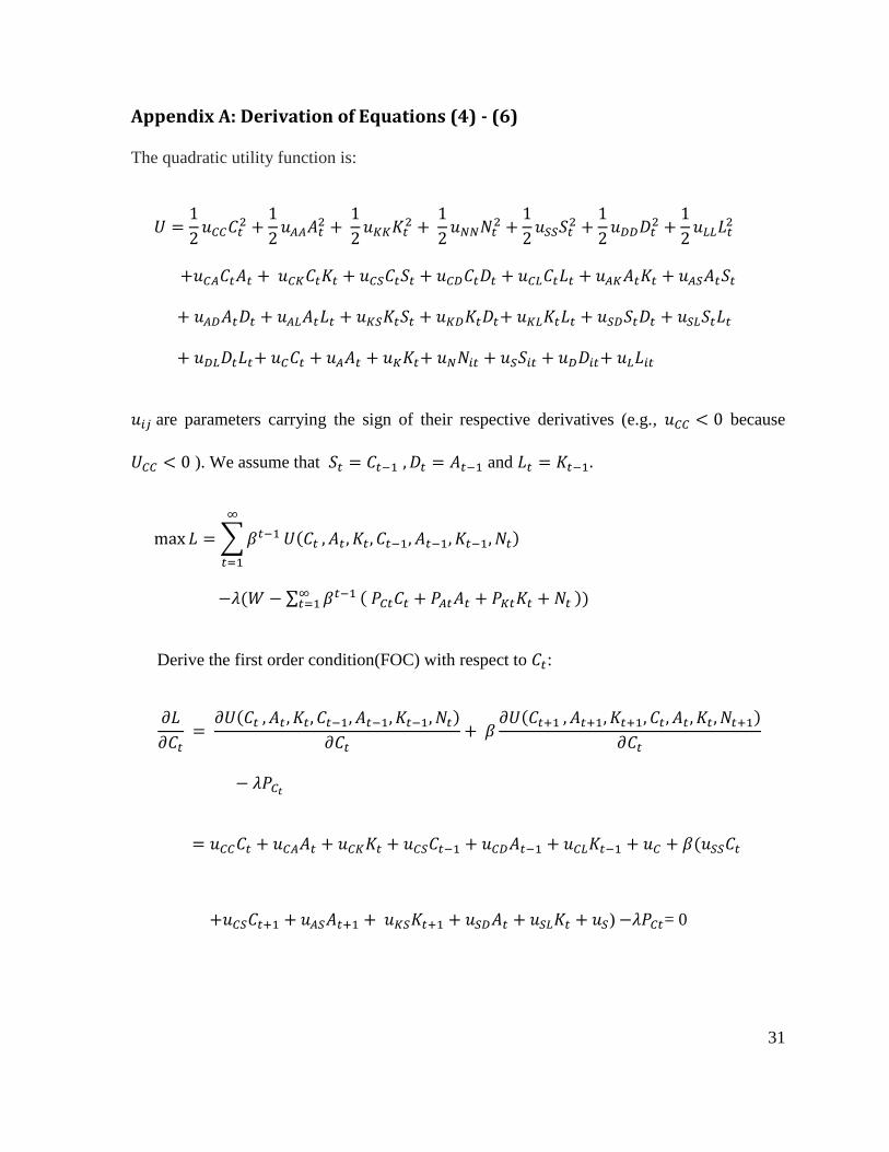
Appendix A: Derivation of Equations (4) - (6)
The quadratic utility function is:
are parameters carrying the sign of their respective derivatives (e.g., because
). We assume that and
Derive the first order condition(FOC) with respect to :
) = 0
32
Solving FOC for :
where
Solving FOC
, for
where

33
Solving FOC
, for
where
For k=1,2,3: or since β=
with r being
discount rate.

34
Appendix B: Calculation of Lewbel Price Indices for Alcoholic Beverages
Lewbel price indices allow heterogeneity in preferences within a given bundle of goods.
Within bundle Cobb Douglas preferences are assumed, while among different bundles any
specification is allowed. See Lewbel(1989) for details. Following Lewbel (1989) and
Hoderlein and Mihaleva (2008), we construct Lewbel price indices as:
where is the household’s budget share of good j in group i. is a scaling factor with
and is the budget share of the reference household.
Let where is the price index for group i which is set to 1 in the first time
period. Because there are zero expenditures for some subcategories, Lewbel price index
cannot be used in levels (i.e., a number divided by zero is undefined). In the empirical
analysis, Hoderlein and Mihaleva(2008) used log prices instead of prices in levels using the
result that In our economic model, prices are in levels, so we first
took the log of the Lewbel price index and then took the anti-log of it to obtain price indices.
In the current study, zero alcohol consumption might be due to so many different reasons
such as quiting, abstention, corner solution and infrequency of purchase. For non-consumers,
the Lewbel price index is assigned to be equal to 1 which means if the consumption took
place, the expenditure shares would have been identical to that of reference household. To
determine the expenditure shares of the reference household, we took the average of the
expenditure shares for each consumer unit in the whole sample in the whole sample period.


