
Principles of Interferometry Hans-Rainer Klöckner IMPRS Black Board Lectures 2014
acknowledgement § Mike Garrett lectures § James Di Francesco crash course lectures § Greg Taylor lecture § NRAO Summer School lectures § Phil Diamond ICRAR § Ger de Bruyn SKADS workshop

Lecture 2 § radio astronomical terms and definitions § antenna temperature § single dish telescope type § single dish telescope beams § sensitivity § basic calibration

Maxwell Equations
vacuum equations
Poynting vector energy flux of an electro-magnetic wave
S = c/4pi E x B [W m-2]

vector waves

polarised wave
degree of polarisation Stokes parameter

brightness temperature black body • Properties of “black-body radiation” (you should all be familiar with this!)
- functional form is called the “Planck function”:
(1)
Radio photons are pretty wimpy:
(2)
• Eqn(2) is known as the Raleigh-Jeans law i.e. at low frequencies the intensity increases with the square of the frequency.
Note that the R-J law holds all the way through the radio regime for any reasonable temperature
k is boltzmann’s constant = 1.38E-23 m2 kg s-2 K-1
Units of spectral energy density are Watts per Hz
per sq. metre per steradian
Rayleigh-Jeans Law
Basic terms and formulae
4

Radio imaging
Radio photons are too wimpy to do very much - we cannot usually detect individual photons
- e.g. optical photons of 600 nanometre => 2 eV or 20000 Kelvin (hv/kT)
- e.g. radio photons of 1 metre => 0.000001 eV or 0.012 Kelvin
! Photon counting in the radio is not usually an option, we must think classically in terms of measuring the source electric field etc.
i.e. measure the voltage oscillations induced in a conductor (antenna) by the incoming EM-wave. Example:
Radio Telescopes (Antennas)
Detector
Cable
Reflector
Feed horn
Amplifier
9
Nyquist law
A resistor (even without current) at temperature T produce noise power Pν dν = kT dν
assume one could connect the resistor to the telescope without any loss one would measure the telescope temperature

surface brightness & flux density
EM power in bandwidth !"!from solid angle !#!intercepted by surface !$ is:
Intensity & Flux Density
!
"W = I#"$"A"#Defines surface brightness Iv (W m-2 Hz-1 sr-1 ; aka specific intensity)
!
Sv = Lv /4"d2 ie. distance dependent#$1/d2 % I& $ Sv /# ie. distance independent
Note:
Flux density Sv (W m-2 Hz-1) – integrate brightness over solid angle of source
Convenient unit – the Jansky ! 1 Jy = 10-26 W m-2 Hz-1 = 10-23 erg s-1 cm-2 Hz-1
!
Sv = Iv" s# d"
Basic Radio/mm Astronomy

brightness temperature - source
Many astronomical sources DO NOT emit as blackbodies! However….
Brightness temperature (TB) of a source is defined as the temperature of a blackbody with the same surface brightness at a given frequency:
This implies that the flux density
Brightness Temperature
!
Sv = Iv" s# d" =
2kv 2
c 2TBd"#!
I" =2kv 2TBc 2
Basic Radio Astronomy

What does a Radio Telescope detect
Recall :
!
"W = I#"$"A"#
!
Prec =12I" Ae#$
Telescope of effective area Ae receives power Prec per unit frequency from an unpolarized source but is only sensitive to one mode of polarization:
Telescope is sensitive to radiation from more than one direction with relative sensitivity given by the normalized antenna pattern PN(!,"):
!
Prec =12Ae I" (#,$)PN (#,$)
4%& d'
Basic Radio Astronomy
What does a Radio Telescope Detect?

brightness temperature - telescope
In general surface brightness is position dependent, ie.!!! "!!!#",#$!
(if I! described by a blackbody in the Rayleigh-Jeans limit; h!/kT << 1)
Back to flux:
In general, a radio telescope maps the temperature distribution of the sky
!
Sv = Iv (" s# $,%)d" =
2kv 2
c 2T($,%)d"#
!
I" (#,$) =2kv 2T(#,$)
c 2
Basic Radio/mm Astronomy
Surface Brightness

measurement
Sν =2k
AeffTA
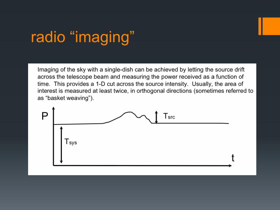
radio “imaging”

radio telescope

primary antenna key features

origin of the beam pattern

antenna power pattern
J1 Bessel Function

the beam P(θ,φ,ν) = A(θ,φ,ν) I(θ,φ,ν) Δν ΔΩ effective collecting area A(ν,θ,φ) [m2] on-axis response
A0 = η A η = aperture efficiency Normalized pattern (primary beam) A(ν,θ,φ) = A(ν,θ,φ)/A0 Beam solid angle ΩA= ∫∫ A(ν,θ,φ) dΩ all sky A0 ΩA = λ2 λ = wavelength, ν = frequency

a real beam

reflector types
Prime focus Cassegrain focus (GMRT) (AT) Offset Cassegrain Naysmith (VLA) (OVRO) Beam Waveguide Dual Offset (NRO) (ATA)

antenna mount

polarisation
Antenna can modify the apparent polarisation properties of the source: § Symmetry of the optics § Quality of feed polarisation splitter § Circularity of feed radiation patterns § Reflections in the optics § Curvature of the reflectors § paralactic angle - mount dependent

pointing accuracy
Pointing Accuracy Δθ = rms pointing error Often Δθ < θ3dB /10 acceptable Because A(θ3dB /10) ~ 0.97 BUT, at half power point in beam A(θ3dB /2 ± θ3dB /10)/A(θ3dB /2) = ±0.3 For best VLA pointing use Reference Pointing. Δθ = 3 arcsec = θ3dB /17 @ 50 GHz
Δθ
θ3dB
Primary beam A(θ)

focal plane arrays
8
Focal Plane Arrays
9
8x8 FPA in WSRT prime focus
APERTIF = APERture Tile In Focus
Increasing the surveying speed by a factor ~ 5 - 25 (depends on Tsys)

antenna performance

importance of antenna element within an interferometer
§ Antenna amplitude pattern causes amplitude to vary across the source.
§ Antenna phase pattern causes phase to vary across the source. § Polarisation properties of the antenna modify the apparent
polarisation of the source. § Antenna pointing errors can cause time varying amplitude and
phase errors. § Variation in noise pickup from the ground can cause time variable
amplitude errors. § Deformations of the antenna surface can cause amplitude and
phase errors, especially at short wavelengths.

observing

calibrate basic step 1
problem is that we do not know Aeff in general
hot = absorbing material (300 K) cold = soaked in liquid nitrogen (77 K)
Sν =2k
AeffTA
relate the voltages measured at the receiver system to the antenna temperature
receiver system need to be linear
for a horn antenna Aeff can be calculated analytical now we can relate source flux density with antenna temperature

calibrate basic step 2
hot = absorbing material (300 K) cold = soaked in liquid nitrogen (77 K)
Sν =2k
AeffTA
know flux density of the source can be use to calibrate other telescope
receiver system need to be linear
antenna temperature for another telescope
40 Jy

calibrate routine work with the known parameters of a telescope we can simply bootstrap the flux densities of sources to be measured. All we need is a calibration source not too far away from the target source
calibrator voltage and flux density
target voltage

sensitivity (noise)

radiometer equation

nice example When Penzias & Wilson (see lecture 1) made their measurements, they found:
Tatm = 2.3 +/- 0.3 K,
Tloss = 0.9 +/- 0.4 K,
Tspill < 0.1 K.
And they expected Tsky ~ 0.
So looking straight up, they expected to measure TA,
TA = 2.3 + 0.9 + 0.1 + 0 = 3.2 K.
What they found was TA = 6.7 Kelvin!
The excess was the CMB and Galactic emission.
Bell lab advert (right) - 1963 - 3 years before the CMB was detected - and featuring the Penzias & Wilsons horn antenna.


