
1

PRICING DEFAULT AND FINANCIAL DISTRESS RISKS IN FOREIGNCURRENCY-DENOMINATED CORPORATE LOANS IN TURKEY
A THESIS SUBMITTED TOTHE GRADUATE SCHOOL OF APPLIED MATHEMATICS
OFMIDDLE EAST TECHNICAL UNIVERSITY
BY
AYCAN YILMAZ
IN PARTIAL FULFILLMENT OF THE REQUIREMENTSFOR
THE DEGREE OF MASTER OF SCIENCEIN
FINANCIAL MATHEMATICS
SEPTEMBER 2011

Approval of the thesis:
PRICING DEFAULT AND FINANCIAL DISTRESS RISKS IN FOREIGN
CURRENCY-DENOMINATED CORPORATE LOANS IN TURKEY
submitted by AYCAN YILMAZ in partial fulfillment of the requirements for the degreeof Master of Science in Department of Financial Mathematics, Middle East TechnicalUniversity by,
Prof. Dr. Ersan AkyıldızDirector, Graduate School of Applied Mathematics
Assoc. Prof. Dr. Omur UgurHead of Department, Financial Mathematics
Assoc. Prof. Dr. Isıl ErolSupervisor, Department of Economics, METU
Examining Committee Members:
Assoc. Prof. Dr. Omur UgurDepartment of Financial Mathematics, METU
Assoc. Prof. Dr. Isıl ErolDepartment of Economics, METU
Assoc. Prof. Dr. Azize HayfaviDepartment of Financial Mathematics, METU
Date:
∗ Write the country name for the foreign committee member.

I hereby declare that all information in this document has been obtained and presentedin accordance with academic rules and ethical conduct. I also declare that, as requiredby these rules and conduct, I have fully cited and referenced all material and results thatare not original to this work.
Name, Last Name: AYCAN YILMAZ
Signature :
iii

ABSTRACT
PRICING DEFAULT AND FINANCIAL DISTRESS RISKS IN FOREIGNCURRENCY-DENOMINATED CORPORATE LOANS IN TURKEY
Yılmaz, Aycan
M.S., Department of Financial Mathematics
Supervisor : Assoc. Prof. Dr. Isıl Erol
September 2011, 116 pages
The globalization leads to integration of the economies worldwide. As the firms’ businesses
also get integrated with each other, the financing choices of the firms diversify. Among these
choices, the popularity and the share of foreign currency borrowing in total borrowing by
non-financial firms increase in Turkey similar to the global developments. The main purpose
of this thesis is to price the risks of default and financial distress due to foreign currency de-
nominated loans of non-financial firms in Turkey. The valuation model of foreign currency
corporate loans is established by two state variable option pricing model based on the study
of Cox, Ingersoll and Ross [28]. In our model, the main risk factors are identified as the ex-
change rate and the interest rate, which are the state variables of the main partial differential
equation whose solution gives the value of the asset. The numerical results are tested for dif-
ferent parameters and for different economic environments. The findings show that interest
rate fluctuations are more important both for the default and financial distress option values
than the fluctuations in exchange rate. However, the effect of upside movements of exchange
rate on the financial distress and default values is sharper than the downside movement effect
of interest rate. Furthermore, high loan-to-value (LTV) foreign currency loans result in signif-
iv

icantly high financial distress values that cannot be disregarded and can lead to default of the
firm. To the best of our knowledge, this thesis is the first study that develops a structural model
to evaluate foreign currency denominated corporate loans in an option-pricing framework.
Keywords: Foreign Currency Denominated Corporate Loans, Bankruptcy, Financial Distress,
Explicit Finite Difference Method, Capital Structure
v

OZ
TURKIYE’DE DOVIZ CINSINDEN KURUMSAL KREDILERIN IFLAS VE MALISIKINTI RISKLERININ FIYATLANDIRILMASI
Yılmaz, Aycan
Yuksek Lisans, Finansal Matematik Bolumu
Tez Yoneticisi : Doc. Dr. Isıl Erol
Eylul 2011, 116 sayfa
Kuresellesme, ekonomilerin dunya genelinde butunlesmesine yol acmaktadır. Firmaların
isleri de butunlestikce, firmaların finansman secenekleri cesitlenmektedir. Bu secenekler
arasında, Turkiye’deki finansal olmayan sirketlerin toplam borclanmaları icindeki yabancı
para cinsinden borclanmalarının payı ve populeritesi kuresel gelismelere benzer sekilde art-
maktadır. Bu tezin temel amacı Turkiye’deki finansal olmayan sirketlerin yabancı para cinsin-
den borclanmalarından kaynaklanan iflas ve mali sıkıntının fiyatlandırılmasıdır. Yabancı para
cinsinden kurumsal kredilerin degerleme modeli Cox, Ingersoll ve Ross’un [28] calısması
uzerine dayandırılaran iki durum degiskenli opsiyon fiyatlama modeliyle kurulmustur. Bizim
modelimizdeki temel risk faktorleri, cozumu varlık degerini veren ana kısmi diferansiyel den-
klemin durum degiskenleri olan doviz kuru ve faiz oranı olarak belirlenmistir. Numerik
sonuclar farklı parametreler ve farklı ekonomik cevreler icin test edilmistir. Bulgular faiz
oranındaki dalgalanmaların, iflasın ve mali sıkıntının her ikisinin degeri icin doviz kurun-
daki dalgalanmalardan daha onemli oldugunu gostermektedir. Ancak, doviz kurunun mali
sıkıntı ve iflas degerleri uzerindeki yukarı hareketlerinin etkisi faiz oranının asagı hareketinin
etkisinden daha keskindir. Ayrıca, yuksek yabancı para cinsinden kredi/deger oranları goz
vi

ardı edilemeyecek degerleriyle mali sıkıntıya neden olmaktadır ve firmanın iflas etmesine yol
acabilir. Bildigimiz kadarıyla, bu calısmanın katkısı, yabancı para cinsinden kurumsal kredi-
lerin bir modelini yapısal opsiyon fiyatlama modeli cercevesinde gelistiren ve degerleyen ilk
olması acısından ayırt edilir ozelliktedir.
Anahtar Kelimeler: Doviz Cinsinden Kurumsal Krediler, Iflas, Mali Sıkıntı, Acık Sonlu Fark-
lar Yontemi, Sermaye Yapısı
vii

To my family,
viii

ACKNOWLEDGMENTS
I would like to express my gratitude to my supervisor Assoc. Prof. Dr. Isıl Erol for introduc-
ing me the topic, for her guidance, motivation and encouragment during this study.
I am grateful to Assoc. Prof. Dr. Azize Hayfavi for her valuable lectures and support during
my graduate study. I am also very grateful to Assoc. Prof. Dr. Omur Ugur for his comments
and support.
I am very thankful to my managers and my colleagues for their understanding and support.
I would also like to thank to my friends who listened and encouraged me all the way.
I wish to express my sincere gratitude to my family for their love, for always trusting and
supporting me throughout my life.
ix
TABLE OF CONTENTS
ABSTRACT . . . . . . . . . . . . . . . . . . . . . . . . . . . . . . . . . . . . . . . . iv
OZ . . . . . . . . . . . . . . . . . . . . . . . . . . . . . . . . . . . . . . . . . . . . . vi
DEDICATION . . . . . . . . . . . . . . . . . . . . . . . . . . . . . . . . . . . . . . viii
ACKNOWLEDGMENTS . . . . . . . . . . . . . . . . . . . . . . . . . . . . . . . . . ix
TABLE OF CONTENTS . . . . . . . . . . . . . . . . . . . . . . . . . . . . . . . . . x
LIST OF TABLES . . . . . . . . . . . . . . . . . . . . . . . . . . . . . . . . . . . . xiii
LIST OF FIGURES . . . . . . . . . . . . . . . . . . . . . . . . . . . . . . . . . . . . xv
CHAPTERS
1 INTRODUCTION . . . . . . . . . . . . . . . . . . . . . . . . . . . . . . . 1
1.1 Introduction . . . . . . . . . . . . . . . . . . . . . . . . . . . . . . 1
1.2 General Overview of the Credit Market . . . . . . . . . . . . . . . . 2
1.3 Motivation for the Research . . . . . . . . . . . . . . . . . . . . . . 3
1.4 Research Content and Methodology . . . . . . . . . . . . . . . . . . 4
1.5 Organization of the Thesis . . . . . . . . . . . . . . . . . . . . . . . 5
2 LITERATURE REVIEW . . . . . . . . . . . . . . . . . . . . . . . . . . . . 7
2.1 Introduction . . . . . . . . . . . . . . . . . . . . . . . . . . . . . . 7
2.2 Foreign Exchange Loan Market . . . . . . . . . . . . . . . . . . . . 7
2.3 Why Do Firms Issue Foreign Currency Denominated Debt? . . . . . 9
2.4 Risks Associated with Foreign Currency Debt Issuance . . . . . . . 12
2.5 Pricing of Risky Debt . . . . . . . . . . . . . . . . . . . . . . . . . 13
3 CURRENCY LOAN VALUATION . . . . . . . . . . . . . . . . . . . . . . 17
3.1 Introduction . . . . . . . . . . . . . . . . . . . . . . . . . . . . . . 17
3.2 Contingent Claims Valuation Framework . . . . . . . . . . . . . . . 17
x

3.2.1 Exchange Rate and Term Structure of Interest Rate . . . . 17
3.3 The Foreign Currency Denominated Loan Contract . . . . . . . . . 19
3.3.1 Notations . . . . . . . . . . . . . . . . . . . . . . . . . . 19
3.3.2 Valuation of Monthly Payments . . . . . . . . . . . . . . 20
3.3.3 Valuation of Future Payments . . . . . . . . . . . . . . . 20
3.3.4 Value of the Loan . . . . . . . . . . . . . . . . . . . . . . 21
3.3.5 Value of the Default Option . . . . . . . . . . . . . . . . . 22
3.3.6 Valuation of Financial Distress . . . . . . . . . . . . . . . 22
4 NUMERICAL SOLUTION OF A TWO-STATE VARIABLE CONTINGENTCLAIMS VALUATION MODEL USING THE EXPLICIT FINITE DIFFER-ENCE METHOD . . . . . . . . . . . . . . . . . . . . . . . . . . . . . . . . 24
4.1 Introduction . . . . . . . . . . . . . . . . . . . . . . . . . . . . . . 24
4.2 The Finite Difference Methodology . . . . . . . . . . . . . . . . . . 25
4.2.1 Finite Difference Approximations . . . . . . . . . . . . . 25
4.3 A Framework for the Solution of the Model Using an Explicit FiniteDifference Method . . . . . . . . . . . . . . . . . . . . . . . . . . . 28
4.3.1 Transformed Version of the Original PDE . . . . . . . . . 28
4.3.1.1 Consistency, Stability and Convergence of theNumerical Procedure . . . . . . . . . . . . . 30
4.3.2 Finite Difference Representation of the PDE . . . . . . . . 32
4.3.2.1 Interior Points . . . . . . . . . . . . . . . . . 32
4.3.2.2 Upper Boundary Conditions in the TransformedState Variables . . . . . . . . . . . . . . . . . 33
4.3.2.3 Lower Boundary Conditions in the TransformedState Variables . . . . . . . . . . . . . . . . . 34
4.3.2.4 Corners of the Grid . . . . . . . . . . . . . . 35
5 ANALYSIS OF THE FOREIGN CURRENCY LOAN VALUATION MODELRESULTS . . . . . . . . . . . . . . . . . . . . . . . . . . . . . . . . . . . . 37
5.1 Introduction . . . . . . . . . . . . . . . . . . . . . . . . . . . . . . 37
5.2 Overview of the Valuation Functions . . . . . . . . . . . . . . . . . 38
5.3 Mathematical Interpretations of the Model . . . . . . . . . . . . . . 39
5.3.1 Interest Rate Volatility . . . . . . . . . . . . . . . . . . . 39
5.3.2 Exchange Rate Volatility . . . . . . . . . . . . . . . . . . 40
xi

5.3.3 Correlation Between Wiener Processes . . . . . . . . . . . 41
5.3.4 Initial Loan to Value Ratio . . . . . . . . . . . . . . . . . 41
5.3.5 Financial Distress Barrier . . . . . . . . . . . . . . . . . . 42
5.4 Financial Implications of the Model . . . . . . . . . . . . . . . . . . 42
5.4.1 Effect of LTV Ratio . . . . . . . . . . . . . . . . . . . . . 44
5.4.2 Effect of Volatilities . . . . . . . . . . . . . . . . . . . . . 44
6 CONCLUSION . . . . . . . . . . . . . . . . . . . . . . . . . . . . . . . . . 69
6.1 Summary . . . . . . . . . . . . . . . . . . . . . . . . . . . . . . . . 69
6.2 Contributions of the Research and Further Study . . . . . . . . . . . 71
REFERENCES . . . . . . . . . . . . . . . . . . . . . . . . . . . . . . . . . . . . . . 73
APPENDICES
A Matlab Code for Consistency, Stability and Convergence of the TransformedPDE . . . . . . . . . . . . . . . . . . . . . . . . . . . . . . . . . . . . . . . 76
B Matlab Code for Loan Valuation . . . . . . . . . . . . . . . . . . . . . . . . 80
xii

LIST OF TABLES
TABLES
Table 5.1 Base Values . . . . . . . . . . . . . . . . . . . . . . . . . . . . . . . . . . 55
Table 5.2 Total Liabilities to Total Assets Ratio . . . . . . . . . . . . . . . . . . . . 56
Table 5.3 Changes in Volatility of Interest Rate ( f = 1.8996) . . . . . . . . . . . . . 57
Table 5.4 Changes in Volatility of Interest Rate ( f = 2.2388) . . . . . . . . . . . . . 58
Table 5.5 Changes in Volatility of Exchange Rate ( f = 1.8996) . . . . . . . . . . . . 59
Table 5.6 Changes in Volatility of Exchange Rate ( f = 2.2388) . . . . . . . . . . . . 60
Table 5.7 Changes in Correlation Coefficient ( f = 1.8996) . . . . . . . . . . . . . . 61
Table 5.8 Changes in Correlation Coefficient ( f = 2.2388) . . . . . . . . . . . . . . 62
Table 5.9 Changes in LTV Ratio ( f = 1.8996) . . . . . . . . . . . . . . . . . . . . . 63
Table 5.10 Changes in LTV Ratio ( f = 2.2388) . . . . . . . . . . . . . . . . . . . . . 64
Table 5.11 Changes in LTV Ratio ( f = 2.6534) . . . . . . . . . . . . . . . . . . . . . 65
Table 5.12 Changes in LTV Ratio ( f = 3.1716) . . . . . . . . . . . . . . . . . . . . . 66
Table 5.13 Changes in Financial Distress Barrier ( f = 2.2388) . . . . . . . . . . . . . 67
xiii

Table 5.14 Combined Effects of Th and LTV ratio on Financial Distress ( f = 2.2388) . 68
xiv
LIST OF FIGURES
FIGURES
Figure 5.1 Value of Future Payments (A) (LTV=0.80) . . . . . . . . . . . . . . . . . 47
Figure 5.2 Value of Future Payments (A) (LTV=0.90) . . . . . . . . . . . . . . . . . 48
Figure 5.3 Value of Loan (V) (LTV=0.80) . . . . . . . . . . . . . . . . . . . . . . . 49
Figure 5.4 Value of Loan (V) (LTV=0.90) . . . . . . . . . . . . . . . . . . . . . . . 50
Figure 5.5 Value of Financial Distress (FD) (LTV=0.80) . . . . . . . . . . . . . . . 51
Figure 5.6 Value of Financial Distress (FD) (LTV=0.90) . . . . . . . . . . . . . . . 52
Figure 5.7 Value of Default (D) (LTV=0.80) . . . . . . . . . . . . . . . . . . . . . . 53
Figure 5.8 Value of Default (D) (LTV=0.90) . . . . . . . . . . . . . . . . . . . . . . 54
xv

CHAPTER 1
INTRODUCTION
1.1 Introduction
Financing choices of the firms play an important role in their capital structure as these choices
include certain risks. Types of financing that a firm can choose differ along with the risks and
benefits associated with them. Traditional financing types are categorized into two groups;
namely, debt financing and equity financing. Debt financing can be defined as borrowing
money to pay back to the lending party. Loan origination and bond issuance are the two com-
monly used types of debt financing. Corporations often issue debt contracts. As the interest
payment on debt is an expense to produce an income or benefit, it is tax deductible. In par-
ticular, tax-deductible business expenses are subtracted from a company’s income before it
is subject to taxation. By reducing taxable income, these deductions reduce a company’s tax
liability and thus improving its net income. Another advantage of debt financing is that the
lender cannot claim an ownership unless the firm does not pay its obligations. The second tra-
ditional financing is the equity financing in which the money lent in exchange for ownership
in a company. In case financing needs occur for the company, involving investors to the busi-
ness may end with loss of control. Firms generally choose equity financing for their startups
or when they need to raise additional equity capital to compensate the existing debt. Reports
on the corporations’ choices of financing sources, reveal that non-financial firms mainly use
external financing sources, like loan-taking or bond issuance rather than equity financing [1].
1

1.2 General Overview of the Credit Market
In recent years, as the business investments grew, the corporate borrowing has expanded
rapidly. Economic and financial globalization and the expansion of world trade have had
effects on both the financing choice of the firms and the choice of the currency of denomina-
tion in corporate debt issues. Over the time the share of foreign debt in corporate borrowing
has considerably increased. Specifically, in 1983, US firms had foreign currency denomi-
nated debt of around $1 billion which increased to $62 billion in 1998 [2]. In the European
area, there is also an increasing trend in issuing foreign currency denominated credits espe-
cially for the private sector credits [42]. In addition to US and EU countries, in developing
countries foreign currency bond issuance and bank borrowing by corporations rose from $81
billion in 2002 to $423 billion in 2007. Examining the external corporate borrowing in re-
gional base, it is seen that the developing countries raised their share in corporate borrowing
from external sources in all regions defined by the World Bank. According to World Bank’s
Global Development Finance 2009 report [3], Europe and Central Asia, including Turkey,
had the largest share of the foreign currency debt in 2007. In Europe and Central Asia region
corporate borrowing rose to $197 billion in 2007, from $19 billion in 2002. Three main non-
financial sectors that use the biggest portion of foreign debt among the developing-country
corporations are oil & gas, telecommunications, utility & energy sectors.
In align with global developments during the last decade, borrowing in foreign currency has
also increased in Turkey. The share of foreign exchange loans (FX-loans) taken by corporate
sector within the total cash loans was 57% in 2005 which increased to 64% in 2008. This
ratio went down as a result of the exchange rate movements and the 2008 economic crisis
but stayed around 60% levels. Due to the amendment to Decree No. 32 in June 2009, when
firms shifted their credit utilization towards the domestic market. Over the period from 2008
to 2010, foreign currency borrowing from domestic sources continued to increase from $46
billion to $52 billion, whereas foreign borrowing from abroad decreased to $89 billion from
$100 billion. Similar to the global FX-borrowing trends in sectorwise, among ten sectors
listed on the Istanbul Stock Exchange (ISE), Electricity, Gas and Water Sources sub-sector
use mostly FX-loans. FX-loans-to-total loans ratios for those sectors are 90.9%, 93.3% and
94.6% in 2008, 2009 and 2010, respectively [4].
2

The share of FX-loans of corporations in total are increasing significantly both in Turkey
and in almost all economies around the world. Foreign currency debt financing affects the
economic exposure of the firms. Economic exposure is defined as the long-term sensitivity of
a firm’s cash flows to exchange rate changes. A foreign currency transaction is exposed to the
risk of fluctuations in exchange rates. A considerable amount of researches have been made to
investigate the motives lying under the FX-loans issuance by non-financial firms. The results
suggest that the two main reasons to issue foreign currency denominated debt are to hedge
the foreign operations and to benefit from lower financing costs. In addition, transaction costs
of financing, arbitrage differences in tax rates and credit-ratings of firms are the other reasons
for the issuance of foreign currency denominated debt.
Although most countries have regulations for banks to limit their foreign exchange exposure,
banks are still indirectly exposed to that risk due to currency mismatches on their clients’
balance sheets. It is important to note, worldwide standards for the regulation of issuing
foreign currency denominated debt do not exist for the non-financial corporations. However,
considering the potential risks some countries put limitations on FX-loans especially for the
non-financial firms. For instance, with amendment to Decree No. 32, Turkey also puts some
restrictions on foreign currency borrowing both at the household and at the corporate level.
Existing academic literature investigated the main reasons for issuing FX-loans. Furthermore,
the possible financial distress to firms that is created by exchange rate fluctuations is measured
according to stock price performance and operating performance by statistical methods.
1.3 Motivation for the Research
For the companies that are heavily financed by FX-loans, during the life of the loan, the
decrease in borrowing rates and depreciation in domestic currency are the two important risks
to consider. The share of foreign currency denominated corporate loans in non-financial firms’
total borrowing is increasing in recent years despite the risks created by foreign exchange
exposure and financing costs. These risks are especially important because of their potential
effects on capital structure of the firms. Research on credit risk valuation appears in various
works in the existing literature. However, to our knowledge, there has not been a study of
pricing of foreign currency loans and related default and financial risks in a contingent claims
3

framework.
The main objective of this thesis is to develop a contingent claims approach (a structural
model) to evaluate (price) both the foreign-currency risk and the interest rate risk of FX-loans
at the corporate level. In other words, this thesis investigates the financial distress and default
risk of non-financial corporations which are heavily financed by FX-loans. In this framework,
the present study aims at setting the general characteristics of the valuation functions for the
FX-loan and its related assets. Explicitly, the values of future payments, financial distress and
default option, in line with the Turkish corporate credit market conditions.
Our research is developed based on these motivations and contributes to the existing literature
in three ways. First of all, this study organizes the various theories into a single framework
discussing foreign exchange rate exposure information at firm level, and develops a model for
pricing the foreign exchange rate denominated loan pricing using option based approach. Sec-
ondly, in the extant literature two state variable contingent claims approaches in credit pricing
models consider asset value of the firm and interest rate as the underlying state variables.
Introducing the exchange rate as another state variable to these models requires constructing
a partial differential equation (PDE) with three state variables. Making simplifying but fi-
nancially reasonable assumptions, we constructed a PDE with two state variables, which are
exchange rate and interest rate. Finally, in existing studies, two state variable option based
loan pricing methods use CIR process to model the interest rate and Brownian motion to
model the asset price. Therefore, in those methods, the main PDE, whose solution gives the
asset value, is constructed with two state variables following a CIR process and a Brownian
process. In contrast, in our model both underlying variables follow Cox Ingersoll Ross (CIR)
process and the main PDE, whose solution gives value of asset, differs from its counterparts
in the literature.
1.4 Research Content and Methodology
Various techniques are developed to measure and manage credit risk. Credit risk pricing tech-
niques that are classified in three categories are; historical method, intensity based method,
and asset based (contingent claims approach) method [32]. Historical method is mostly used
by rating agencies. The default probabilities are calculated according to the firms’ defaults
4

that occurred in the past and the risk is measured by transition matrices indicating the change
from one rating category to another. In intensity based approach, which is also known as
reduced form model, default time is modeled with stopping time of a hazard rate process.
The main shortcoming of these methods is that the models do not explain why default occurs
and default is modeled as an unexpected event. In contingent claims approach, the default
event is related with the capital structure of the firm and unlike other methods this method
explains why default occurs. Contingent claims approach is also called as structural model in
literature.
The general valuation framework used in this work is based on Cox, Ingersoll and Ross’s
structural model [28]. The corresponding valuation equation provides the value of the assets
under study, given the terminal and boundary conditions of the problem. In the present study,
a two state variable version of the model is used to cope with the two natural sources of un-
certainty associated with the FX-loan, term structure risk and exchange rate risk. All changes
in the term structure of interest rates are assumed to be driven by the evolution of the spot
interest rate. In modeling the financial distress for the firms, the distress threshold is identi-
fied according to the financial leverage ratios of the firms where financial leverage and highly
leveraged firm definitions are used following Opler and Titman’s work [26].
In our calculations, we first determine the terminal and boundary conditions for each asset
studied. Given these terminal and boundary conditions, it is possible to use the model to price
the assets for all the other moments in time, with the exception of those when the terminal
conditions do not apply. The closed form solution for the model is probably impossible to
obtain. Therefore, it is necessary to use a numerical solution technique. The nature of the
problem brings on the choice of an explicit finite difference method. Using this methodology,
a series of simulation results are generated which identifies the sensitivity of the different
assets to changes in various parameters of the model.
1.5 Organization of the Thesis
The organization of this thesis is as follows:
Chapter 1 provides an introduction to the whole work. It gives an intuitive notion of the im-
5

portance of the foreign currency denominated corporate loans and credit markets, introduces
the main purposes of the research and presents the methodological approach used, the content
of the thesis, its structure and organization.
Chapter 2 firstly reviews the developments and growth of current foreign currency credit
market, academic literature on foreign exchange exposure of firms. This chapter also presents
the motives behind issuing foreign currency denominated debts, main risks associated with
that type of debt financing and the contingent claims valuation techniques of debts and related
products.
In Chapter 3, the contingent claims valuation model that is used to price the loan, future
payments, financial distress and default option is developed. As the valuation model does not
have a closed-form solution we use numerical methods to solve it.
Chapter 4 presents the transformations and the overall procedure that is required in order to
reach the numerical solution of the problem.
In Chapter 5, several scenarios for the values of the key parameters, that are interest rate
volatility, exchange rate volatility, correlation coefficient, loan-to-value (LTV) ratios and fi-
nancial distress barrier, of the model are studied and conclusions about the values of the
different assets under study are explained in both financial and mathematical perspectives.
Finally, Chapter 6 concludes the thesis identifying the most important contributions and sug-
gesting areas for further research.
6

CHAPTER 2
LITERATURE REVIEW
2.1 Introduction
This Chapter summarizes the existing studies related to foreign currency borrowing by non-
financial firms. the first section presents a synopsis of the foreign exchange loan market
according to financial reports of the countries. the second section summarizes the main studies
that explain the motivations of issuing foreign currency denominated debt. The third section
provides a discussion on the risks created by foreign currency debt issuance. Finally, the last
section discusses credit-pricing methods.
2.2 Foreign Exchange Loan Market
As the investments grew and businesses get integrated firms evaluate different types of financ-
ing opportunities internationally. The evolution of the shares of foreign currency denominated
debt issuance in corporate borrowing is significant over the world.
The data for foreign debt contracted by developing-country corporations, taken from web-
publications of The World Bank, shows that in developing countries foreign currency bond
issuance and bank borrowing by corporations rose from $81 billion in 2002 to $423 billion
in 2007. As the global financial disorder increased, it fell to $271 billion in 2008. In 2002,
72% of the external borrowing by developing-country corporations was bank loans and this
ratio has risen to 85% in 2008. Weighted portion of the total external debt consists of medium
and long-term contracts. The share of the total medium and long-term external debt held by
7

developing countries reached about 50 percent in 2008, up from 5 percent in 1989. Oil & gas,
telecommunications, utility & energy sectors are the three main non-financial sectors that use
the big portion of foreign debt among the developing-country corporations. Although the
total borrowing is decreased from 2007 to 2008, private sector increased its share in external
corporate borrowing to 75% in 2008 from 70% in 2007 [3].
In regional base, the share of foreign borrowing increases in all regions of the developing
countries. Turkey is located in Europe and Central Asia region. The largest share of the
foreign currency debt in 2007 is issued in Europe and Central Asia (ECA). Also in that region
corporate borrowing rose to $197 billion in 2007, from $19 billion in 2002. South Asia region
has realized the largest percentage increase in corporate borrowing from 2002 to 2007, which
is 10 times more than its value in 2002. As compared to other regions, the rise in FX corporate
borrowing in Latin America & the Caribbean and in East Asia & the Pacific was relatively
humble. In 2008, foreign currency corporate borrowing dropped in all regions, except the
Middle East & North Africa [3].
In Turkey borrowing in foreign currency has also increased in accordance with the foreign
currency borrowing trends in the world. According to the 2009 and 2010 Financial Stability
Reports of CBRT, the share of foreign currency loans within the total cash loans was 58% in
2006. This ratio was 64% in 2008 but went down as a result of the exchange rate movements
and the 2008 economic crisis but stayed in 60% levels in 2009. Foreign currency borrowings
of the corporate sector was $84.4 billion in 2006 which increased to $146.4 billion in 2008
decreased to $142 billion at the end of 2009 and to $141.7 billion in March 2010. Following
the amendment made to Decree Number 32 on June 16, 2009, loans obtained from foreign
branches and affiliates of banks established in Turkey and foreign currency loans obtained
from foreign banks went down by $3.7 billion and $4 billion, respectively by March 2010.
As a result of the amendment, firms have decreased the amounts of loans that they use from
abroad and have chosen for domestic banks to issue FX loans. During the period 2008 to
2010, foreign currency borrowing from domestic sources continued to increase from $46
billion to $52 billion whereas foreign borrowing from abroad decreased to $89 billion from
$100 billion. As a matter of fact, decrease in the total amount of FX loans mostly due to the
decrease in the portion of FX loans obtained from foreign countries [4].
For the 10 sectors listed on the ISE the share of FX corporate loans in total corporate loans is
8

shown in 2010 March Financial Stability Report of CBRT. Among these sectors Transporta-
tion, Storage and Communication and Electricity, Gas and Water Sources sectors continued
to raise their shares of FX loans. And Electricity, Gas and Water Sources sector use mostly
FX loans where its FX loans to Total loans ratio is 90.9%, 93.3% and 94.6% in 2008, 2009
and 2010 respectively [4].
The main terms determining the features of foreign currency contracts are maturity structure
and the borrowing rate. According to May 2009 financial Stability Report of CBRT 70% of
the foreign currency borrowing by corporate sector have maturities medium and long term.
Electricity, Gas and Water Sources sector’s medium and long term foreign borrowing to total
foreign borrowing ratio is 85%. As stated previously in 2008 this ratio is 50% in developing
countries. In Turkey, loan interest rates, both TL denominated and FX denominated, increased
in October 2008 attributable to the global crisis. However, between November 2008 and
November 2009 by the interest rate cuts made by CBRT, they fell below their September
2008 levels. During the same period interest rates of TL denominated loans almost doubled
the interest rates of FX denominated loans.
2.3 Why Do Firms Issue Foreign Currency Denominated Debt?
Previous section demonstrates the growth in foreign currency denominated loan market in
Turkey and in all regions of the world. As the portion of foreign borrowing by non-financial
corporations in total borrowings increases, the topic attracts more attention in academic en-
vironment. In addition to risks associated with borrowing in domestic currency, foreign cur-
rency borrowing induces exchange rate risk to the firms. The foreign exchange exposure
of firms and motivations of the firms to issue a debt with additional risks are examined in
academic literature.
Kıymaz [5] investigates the FX exposure of firms in highly inflationary environment. In this
paper, specifically the following issues are discussed: whether the foreign exchange risk is
priced at the firm level, foreign exchange exposure across industries, comparison of exchange
rate exposure in pre-crisis and post-crisis periods, investigation of the relation between foreign
exchange exposure and magnitude of international operations. The sample of the research
consists of 109 firms traded in ISE. Following the work of Dumas [36] and Adler and Dumas
9

[35] the exchange rate exposure is estimated by the regression coefficient of the value of the
firm on the exchange rate for different states of nature. The findings show that Turkish firms
are highly exposed to foreign exchange risks and their values are significantly influenced
by exchange rate fluctuations. In this article it has been showed that the post-crisis foreign
exchange exposures of all industries seem to be lower than those of pre-crisis. Another result
of this study is that the firms with a higher degree of export and import involvement experience
a greater fx-rate exposure. Solakoglu [37] examines the relationship between exchange rate
exposure and firm-specific factors for Turkish firms between 2001 and 2003. Findings of
this study show that firm size and foreign activities as well as being net-exporters and net
importers are significant affects on foreign exchange exposure.
One of the reasons to issue foreign currency denominated debt is to hedge the foreign op-
erations. Examining the motives behind the use of currency derivatives, Geczy et al.[13]
studied 392 Fortune 500 non-financial firms in 1990. In their study, they also included the
naturally hedged firms, defined as having foreign operations and foreign-denominated debt.
They employ multivariate and univariate tests to identify the determinants of using currency
derivatives. They find out that for naturally hedged firms R&D and short-term liquidity are not
significant determinants whereas these variables are still significant determinants of derivative
use for firms having foreign operations but no foreign currency denominated debt. Thus for-
eign currency denominated debt and currency derivatives can be used as substitutes to hedge
foreign operations for this sample. Therefore firms having revenues in foreign currency may
want to issue foreign currency debt in order to provide hedging of foreign exchange exposure.
Many researchers have examined the relation between the FX exposure of non-financial firms
and the foreign currency debt issuance. Taek Ho Kwon and Sung C. Bae [6] study the Korean
manufacturing firms between 1998 − 2005. They measure the effect of foreign currency bor-
rowing on asymmetric foreign exchange exposure with a regression model. They find strong
evidence that firm’s export ratio (total export to total sales ratio) and dollar denominated debt
ratio (difference between the dollar denominated liabilities and dollar denominated assets over
total assets) are significantly related to the firm’s asymmetric foreign exchange exposure but
in the opposite direction.
Allayannis et al [7] examined the 327 of the largest East Asian non-financial firms’ choice
of using alternative types of loans from 1996 to 1998 as well as the effects of foreign bor-
10

rowing on firms’ performance. The results suggest that ability to manage the currency risk
with foreign cashflows and cash reserves is a determinant to use of foreign currency debt.
An unanticipated result of this study is that they find no evidence suggesting that unhedged
foreign currency debt was the primary cause of the 1997 Asian crisis. This result is attributed
to illiquidity of the derivatives market during the crisis.
Keloharju and Niskanen [8] also studied the determinants of the decision to raise currency
debt. Their sample consists of 44 non-financial Finnish companies listing on Helsinki Stock
Exchange between the years 1985 and 1991. Main drivers of foreign borrowing are tested
by using probit regression framework. The findings show that firms having export to sales
ratio high are most likely to raise foreign currency debt. Hence, they reach to conclusion
that hedging is an important determinant of the currency of denomination decision. Kedia
Mozumdar [2] investigated the same topic for large U.S. firms reported to Compustat. They
also employ probit regression model to test the effects of various determinants on foreign
borrowing and find that foreign borrowing relates with the foreign activity.
Whether the economic exposure of non-financial firms has effects on firms’ debt financing
choice is questioned by Goswami and Shrikhande [1]. In their model they used a discrete
time exchange rate process to explain the data on real world. They showed that the dominant
debt-financing alternative for firms faced with negative economic exposure is foreign currency
debt. Also, Hekman [27], Aliber [9] described the hedging purposes of non-financial firms as
the principal incentive of issuing foreign currency denominated debt.
In addition to mathematical and statistical models, survey studies show that in practice foreign
currency borrowing and currency derivatives is used interchangeably. Bradley&Moles [10]
conducted a survey about the techniques used to manage exchange rate risk among the sample
of non-financial firms of UK. In that survey the results show that more than half of the firms
issue foreign currency debt and match costs with revenues issued in the same currency to
manage exchange rate exposure. Graham & Harvey [14] surveyed with 392 CFOs about
the capital structure. In their survey study questions about debt, equity and foreign debt are
asked. 31% of the survey respondents considered issuing foreign debt for which one of the
most popular reasons is to provide a natural hedge against foreign currency devaluation.
Other than hedging purposes, low interest rates of foreign currency denominated corporate
11

loans relative to domestic interest rates made them more preferable among other alternatives.
Firms that have no cash flows in foreign currency may want to borrow in foreign currency
to reduce their interest costs. Keloharju & Niskanen [8] examined the determinants of the
decision to raise foreign currency denominated debt by among 44 Finnish corporations. In
that study it is specified that one of the reasons for corporations to issue FX denominated debt
is the fact that borrowing in foreign currency may cost less than borrowing in home currency.
Allayannis et al [7] investigate the largest East Asian corporations, Kedia & Mozumdar [2]
study the sample of large US firms and Aliber [9], mentioned the interest rate differential as
one of the incentives for the firms to issue FX denominated debt.
Other than hedging and cost of financing advantages, higher liquidity of the debt market
reduces the transaction costs of financing and affects the foreign debt issuance. Legal regimes
having strong creditor rights also lower the cost of financing. Although, it creates a weak
preference, investors may follow the arbitrage differences in tax rates and that affects the
foreign currency debt issuance. Also, Kedia and Mozumdar [2] find that higher credit-rated
firms issue significantly more foreign debt than lower credit-rated firms. Thus credit rating
can also be showed as the incentive to issue more foreign currency denominated debt.
2.4 Risks Associated with Foreign Currency Debt Issuance
Risks induced by foreign borrowing can have many aspects. The previous section reveals that
non-financial firms may issue foreign currency denominated debt by hedging purposes and to
take advantage of lower financing costs. Related with those findings important risks will be
discussed in this section.
Although most countries have regulations for banks to limit their foreign exchange exposure,
banks are still indirectly exposed to that risk due to currency mismatches on their clients’
balance sheets. As of March 2010, 67% percent of total loans consisted of corporate loans.
In CBRT’s Financial Stability Report, it is stated that the share of corporate lending used
to decrease in the post-crisis period; but these loans have increased in the last quarter of
2009 [4]. To illustrate, during the 1997 Asian financial crisis banks did not exercise careful
credit assessment over foreign exchange risks in their corporate customers [41]. Also, during
2001 the Brazilian currency depreciated about 40% from end of the 2000 to September 2001
12

causing the share of foreign currency debt in total debt to increase. Another example of sharp
increase in exchange rate is Turkish lira to dollar exchange rate, which increased to 1.6 million
in July 2001 from 672 thousand in 2000.
Goldstein and Turner [41] state that in a crisis, widening credit spreads and currency deval-
uations tend to occur at the same time. In such circumstances ”cheap” foreign currency debt
can quickly become very expensive to service and refinance. The case of Korea illustrates
risks of assuming cheap foreign currency financing. The won/yen exchange rate has been
very stable over the past decade. Thus firms could generate large profits by borrowing in
yen at low interest rates and using the proceeds to invest in higher-yielding won-denominated
instruments. However, the financial crisis simultaneously cut firms’ export revenues as global
demand plummeted and put the won under pressure.
On the other hand, the higher exchange rate volatility means that the hedging will be more
expensive hence there will be less hedging. Therefore firms will be more exposed to exchange
rate risk in such a case.
2.5 Pricing of Risky Debt
Using contingent claims approach to price risky debt is first introduced by Black and Sc-
holes [15] in 1973 followed by Merton [16]. Credit pricing models using contingent claims
approach can be classified in two categories: structural models and reduced form models.
Reduced form models assume that a firm can default in any time and the event of default is
independent of the firm’s capital structure. This model is generally used in cases where more
data is available. Also reduced form models do not explain the reasons of the default and
ignores the relation between the economics of the firm and the event of default. The study of
Jarrow and Turnbull [17] is one of the first reduced form models. The structural models on the
other hand define the corporate liability as a function of a firm’s capital structure and time. In
that approach, the reasons behind the default are investigated and implemented to the model.
As mentioned in Chapter 1 in this study structural model will be used to price the default risk
of foreign currency denominated loans.
In the study of ”The Pricing of Options and Corporate Liabilities”, Black and Scholes [15]
13

used contingent claims approach to price risky debt. They defined the value of a corporate
liability as a function of the firm’s value and time. This function satisfies a partial differential
equation, which is also known as Black Scholes PDE. In that model asset value of the firm is
assumed to follow a stochastic Brownian motion and risk free rate is assumed to be constant.
Also, default of a firm is defined as a put option with strike price equals to the face value of
the zero coupon debt and default occurs when the value of the assets of the firm is less than
the face value of the debt.
Merton [16] defined value of the equity as a call option on the assets of a firm and derived
the same solution with Black and Scholes for the debt value by subtracting the call price from
the market value of the assets. Furthermore, in this study Black-Scholes method is applied to
corporate debt, which is zero coupon bond and risk structure of interest rate is presented.
The first studies on the valuation of risky debt applied the contingent claims approach to
zero coupon bonds, which have their only payment at the maturity of the bond. Therefore,
early works on this topic assume that a firm can go bankrupt only at the maturities of the
existing debts. Between the issuance date and maturity, assets of the firm can be lower than
the debt obligation. Black and Cox [18] introduced a valuation model for bonds with safety
covenants. The most important assumption made in this study is to assume that trading takes
place continuously. In this model they defined an absorbing barrier for the value of the assets
of a firm and they let default to occur prior to the maturity when the value of a firm hits this
barrier. In their study default barrier is defined as a constant fraction of the present value of
the promised final payment.
Vasicek [38] combined the Black Scholes model with stochastic interest rate and assumed that
spot interest rate follows a mean reverting lognormal process. This model has two stochastic
factors namely asset value and interest rate where the debt value satisfies a two-state PDE.
Introducing stochastic interest rate to the model provide to measure the effects of changes in
interest rate. However, in Vasicek’s interest rate process spot rates can take negative values,
which is not the case in real world. Also, Shimko, Tejima and Van Deventer [19] attempt
interest rate with a stochastic process and assumed that spot interest rate follows the Ornstein-
Uhlenbeck process. The important characteristic of this model is to take non-zero correlation
between the asset value and the interest rate.
14
Longstaff and Schwartz [20] combined the Shimko, Tejima and Van Deventer’s work with
a constant default threshold assumption. They argue that when the firm value reaches the
predefined constant threshold it is an indicator of a financial distress and financial distress
triggers the default of all of the firm’s debts.
Kim, Ramaswamy and Sundersan [21] considered that the firm could default due to its coupon
obligations before the maturity. They also take interest rate as stochastic and used Cox Inger-
soll Ross process to model the spot interest rate. Besides, they take the operating cash flows
of a firm into account, instead of asset value of a firm and they state that a firm’s bankruptcy
is triggered when the firm’s cash flows are unable to cover its interest obligations.
Ericsson and Reneby [22] and Briys and de Varenne [23] also allowed default to occur prior
to maturity in their models. Briys and de Varenne used stochastic default barrier in their
model, which is an extension of the Black & Cox’s study where both the interest rate and the
default barrier are constant. Leland [24] argued that debt values cannot be determined without
knowing the firm’s capital structure, which triggers the default and bankruptcy. Following
this assumption Leland determined the optimal leverage ratio to declare bankruptcy. Toft &
Prucyk [25] followed Leland [24] work and defined bankruptcy level in the same way.
Opler & Titman [26] studied the relation between the corporate performance and financial
distress. The term financial distress is used interchangeably with being highly leveraged and
they measured leverage with book values of debt divided by the book values of assets. Using
book values instead of market values to identify the leverage ratios avoids the problem of in-
cluding market condition related factors to the model. Their sample contains 46,799 years of
data in the 1972 to 1991 period and it is divided in to two groups; firms in industries experi-
encing poor performance and firms in industries experiencing normal performance. Base year
leverage ratios for those samples are found as 34% and 31% for firms in industries experienc-
ing poor performance and firms in industries experiencing normal performance respectively.
They also defined highly leverage firms as having leverage in deciles 8 to 10.
In option pricing methods the value of assets satisfies a partial differential equation, which
does not have closed form solutions. Therefore, numerical methods are employed to reach
to a solution of the PDE. The most common methods are Monte Carlo method, which is a
forward pricing method and finite difference approximation to the differential equation, which
15

is a backward pricing method. These techniques mostly used by valuing mortgage contracts
in literature. Stanton [39], Kau, Keenan, Muller and Epperson [40], Azevedo-Pereira [32]
used finite difference method to find the numerical solution for the value of the mortgage and
its embedded options.
16

CHAPTER 3
CURRENCY LOAN VALUATION
3.1 Introduction
In this study, foreign currency loan and the related assets are treated as derivative assets. A
derivative is an asset whose value depends on the price of some other assets, the underlyings.
The underlying assets’ random movements can be modeled mathematically by stochastic pro-
cesses. In this chapter, properties of the stochastic processes that the underlying assets follow
are discussed and the main PDE to value the derivative assets is derived. Also, payment
functions of the derivative assets to be valued are covered in this chapter.
3.2 Contingent Claims Valuation Framework
3.2.1 Exchange Rate and Term Structure of Interest Rate
The pattern of interest rates over different time periods for different investment opportunities
is known as the term structure of interest rates. In corporate debt valuation models, major
factors affecting the value of the loan are set as the underlying state variables. Interest rate
and asset price are generally determined as two major risk factors for domestic currency fixed
rate loans. Examining the foreign currency denominated fixed rate loans, the interest rate
and the foreign currency rate are determined as the state variables. Mean reverting square
root stochastic process is used to model both of these state variables. This type of stochastic
processes is used to model the commodities, which are sensitive to short-term oscillations but
tends to revert back to a ”normal” long-term equilibrium level while pushing away from zero.
17

In this context, both interest rate and currency rate are assumed to follow mean reverting
square root diffusion process defined by Cox Ingersoll and Ross, which is also known as CIR
process [28]. The mean reverting square root processes for interest rate and foreign currency
rate are given by the following equations respectively:
dr = κr(θr − r)dt + σr√
rdzr (3.1)
d f = κ f (θ f − f )dt + σ f√
f dz f (3.2)
Here κ is the rate of mean reversion. The greater the mean-reverting parameter value κ, the
greater is the pull back to the equilibrium level. θ is the drift term brings the variable being
modeled back to an equilibrium level. σ is the volatility of the process, which is proportional
to the square root of the interest rate. Standardized Wiener processes for interest rate and for-
eign currency rate are dzr and dz f respectively. Relation between these two Wiener processes
is given as follows:
dzrdz f = ρdt (3.3)
where ρ is the instantaneous correlation coefficient between two Wiener processes.
In this study, loan is considered as a derivative asset and its value is assumed to depend on
the term structure of the interest rate and the foreign exchange rate. Market price of risk
associated with the spot interest rate and exchange rate also affects the value of the loan.
Since exchange rate is a traded asset there is no risk adjustment for that variable. Also, option
pricing theory requires a risk neutral economic environment. Using spot interest rate will
eliminate the market price of risk for the interest rate.
The Feyman-Kac theorem is used to derive the partial differential equation (PDE) for the
value of assets F(r, f , t) whose value is a function of the two state variables defined by the
stochastic processes in (3.1) and (3.2). The following PDE can be derived by this method:
∂F∂t
+κr(θr−r)∂F∂r
+κ f (θ f− f )∂F∂ f
+ρσrσ f√
r√
f∂2F∂r∂ f
+12σ2
r r∂2F∂r2 +
12σ2
f f∂2F∂ f 2 −rF = 0 (3.4)
18

The aim of this study is to determine the values of Financial Distress and Default prior to
maturity. Therefore, backward valuation procedure is used in an iterative way. Once the value
of different assets is known at maturity, it is possible to use equation (3.4) to solve for the
value of these assets in previous moments in time. Small time steps backwards were used
to solve the equation giving the value of the loan and loan related assets immediately after
the previous payment date. According to the values obtained in previous steps, new terminal
conditions are determined and this process is repeated iteratively in the life of the loan until
the initial moment and the value of these assets at origination is determined.
3.3 The Foreign Currency Denominated Loan Contract
3.3.1 Notations
The study considers fixed rate foreign currency denominated corporate loans and the follow-
ing notations will be used:
n = life of the loan in months
L = initial amount of loan in domestic currency terms
c = the fixed rate coupon rate
η(i) = ith payment date
fint = fx rate at the origination of the loan
M = monthly payment in foreign currency
VA = book value of the assets of a company
Th = threshold for the financial distress
VB(r, f , t) = Value at time t of the loan for borrower
A(r, f , t) = Value at time t of the remaining payments of the loan
FD(r, f , t) = Value at time t of the financial distress
D(r, f , t) = Value at time t of the default
F−(r, f , t) = Value of the asset F immediately before the payment
F+(r, f , t) = Value of the asset F immediately after the payment
19

3.3.2 Valuation of Monthly Payments
The PDE (3.4) will be solved using a backward procedure. In that context, identifying the
monthly payments of the fixed rate foreign currency denominated loan is necessary for the
valuation procedure. At the origination of the loan, all payables are determined in foreign
currency units. At payment dates, amounts in domestic currency are calculated using the
relevant exchange rates.
The principal that is in foreign currency terms should be paid in full by the end of the contract.
The loan under study is a fixed rate loan therefore during the life of the loan the monthly
payments are same in foreign currency terms.
On the other hand, the borrower gets the loan in domestic currency at the origination date
and makes the monthly payments in domestic currency. Since the exchange rate changes on
payments dates monthly payments can be expressed with the following equation:
M =( c
12 )(1 + c12 )n
(1 + c12 )n − 1
L1fint
(3.5)
3.3.3 Valuation of Future Payments
Valuation of future payments is similar to the valuation of foreign currency denominated
bonds. Given the cash flows, its value is a function of both interest rate and exchange rate
similar to other financial assets. Since the value depends on exchange rate, payments should
be adjusted with the relative rate at each payment date.
By the end of the loan, value of the payment due will be the same as the last monthly payment
adjusted according to the domestic currency. The terminal condition for the value of the future
payments can be defined as follows:
A−(r, f , t) = M f for t = η(n) (3.6)
After each monthly payment the present value of borrower’s debt is reduced by M f . Consid-
ering this the following terminal condition should be used for the other payment dates:
20

A−(r, f , t) = A+(r, f , t) + M f for t = η(1), ..., η(n-1) (3.7)
3.3.4 Value of the Loan
The corporate loan in this study has a probability of default, which makes the value of the
debt risky. The value of the risky debt is defined as the default free value of the debt minus
the expected loss. Expected loss of the debt is an implicit put option on the assets of a firm
[43]. Following the definition, value of the loan can be expressed as follows:
VB = A − D (3.8)
Value of future payments and value of default are affected by two state variables namely
exchange rate and interest rate. Therefore, the value of the loan is also a function of these two
state variables. As mentioned earlier, value of the assets of a firm is assumed to be constant
and value of remaining payments depends on exchange rate and interest rate. Fluctuation in
the state variables affects the value of the future payments and if the amount that the firm is
obliged to pay is more than the value of its assets then the firm goes to bankruptcy. In that
case lender of the loan can get as much as VA, the value of the firm’s assets. So, value of the
debt can be at most VA. At the last payment date the firm can either make the last payment or
goes to bankruptcy. Hence the value at termination is given by,
V−B (r, f , t) = min(M f ,VA) for t = η(n) (3.9)
Following the same logic, value of the debt immediately before the other payment dates is as
follows:
V−B (r, f , t) = min([V+B (r, f , t) + M f ],VA) for t = η(1), ..., η(n-1) (3.10)
21
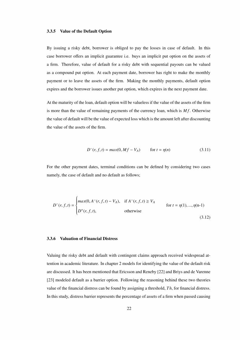
3.3.5 Value of the Default Option
By issuing a risky debt, borrower is obliged to pay the losses in case of default. In this
case borrower offers an implicit guarantee i.e. buys an implicit put option on the assets of
a firm. Therefore, value of default for a risky debt with sequential payouts can be valued
as a compound put option. At each payment date, borrower has right to make the monthly
payment or to leave the assets of the firm. Making the monthly payments, default option
expires and the borrower issues another put option, which expires in the next payment date.
At the maturity of the loan, default option will be valueless if the value of the assets of the firm
is more than the value of remaining payments of the currency loan, which is M f . Otherwise
the value of default will be the value of expected loss which is the amount left after discounting
the value of the assets of the firm.
D−(r, f , t) = max(0,M f − VA) for t = η(n) (3.11)
For the other payment dates, terminal conditions can be defined by considering two cases
namely, the case of default and no default as follows;
D−(r, f , t) =
max(0, A−(r, f , t) − VA), if A−(r, f , t) ≥ VA
D+(r, f , t), otherwisefor t = η(1), ..., η(n-1)
(3.12)
3.3.6 Valuation of Financial Distress
Valuing the risky debt and default with contingent claims approach received widespread at-
tention in academic literature. In chapter 2 models for identifying the value of the default risk
are discussed. It has been mentioned that Ericsson and Reneby [22] and Briys and de Varenne
[23] modeled default as a barrier option. Following the reasoning behind these two theories
value of the financial distress can be found by assigning a threshold, Th, for financial distress.
In this study, distress barrier represents the percentage of assets of a firm when passed causing
22

a financial distress and leading to default. In case of default firm is still in a distress situation
and the value of distress is the difference between the value of remaining payments and the
barrier.
A firm is assumed to be in financial distress when the value of the remaining payments of
the currency denominated debt exceeds the distress barrier. Terminal conditions for the value
of financial distress are similar to the conditions given for default. At termination, if the last
monthly payment exceeds the barrier the firm is assumed to be in financial difficulty with the
amount of the difference between these two values. Monthly payment for the current month
is converted to domestic currency. Hypothetically exchange rate can go to infinity and in this
case value of the option should also go to infinity. In such a case this problem is eliminated
by assuming that firm’s distress value is the difference between the value of the firm’s assets
and the threshold.
FD−(r, f , t) = max(0,M f − Th) for t = η(n) (3.13)
At other payment dates, comparing the value of the remaining payments with the barrier
distress value can be identified and the terminal conditions are given by;
FD−(r, f , t) =
max(0, A−(r, f , t) − Th), if A−(r, f , t) ≥ Th
FD+(r, f , t), otherwisefor t = η(1), ..., η(n-1)
(3.14)
23

CHAPTER 4
NUMERICAL SOLUTION OF A TWO-STATE VARIABLE
CONTINGENT CLAIMS VALUATION MODEL USING THE
EXPLICIT FINITE DIFFERENCE METHOD
4.1 Introduction
Derivative assets can be modeled by partial differential equations (PDEs) in contingent claims
analysis framework. Most of the PDEs used in finance can be categorized in first order lin-
ear equations and second order linear parabolic equations that allow addopting mathematical
methods to real world finance problems [30]. This chapter presents a numerical procedure
for the solution of a contingent claims valuation model in order to value the assets related to
foreign currency denominated loans. Considering the nature of those assets and the informa-
tion available at the origination of the contract, backward valuation procedure is used. The
most commonly used types of backward procedures are lattices and finite difference methods
in which finite difference methods are able to compute simultaneously several starting contin-
gent claim prices for different values of the risk parameters and can be more powerful when
several option values are to be calculated simultaneously [31]. The boundary and terminal
conditions necessary for the solution of the model are described according to the cash-flow
structure of the asset under valuation.
24

4.2 The Finite Difference Methodology
In the finite difference methods the domain of the problem is divided into a grid and the PDE
is discretized by replacing each partial derivative with a difference quotient. Discretizing the
PDE the derivative terms are approximated by replacing them with the respective finite dif-
ference approximations that approximate their values between the nodes obtained. The finite
difference equivalents of the derivative terms are derived from the Taylor series expansions.
4.2.1 Finite Difference Approximations
Let u(x) be a continuous function of the single independent variable x, the x domain is dis-
cretized into a grid. The constant grid spacings in the x and t directions are given by h and k.
In one-dimensional problems the function of any grid point is given by:
u(xi) ≡ u(ih) ≡ ui for i = 0, 1, 2, ... (4.1)
Uni and un
i are the difference and differential equations respectively at the points x = ih and
t = nk .
In two-space-dimensional problems, grid spacings for x direction are given by h and grid
spacings for y direction are given by l. The function for any grid point is represented as
follows:
u(y j, xi) ≡ u( jl, ih) ≡ u j,i for i = 0, 1, 2, ... and j = 0, 1, 2, ... (4.2)
The representation of the difference and differential equations at the point x = ih, y = jl and
t = mk will be denoted by Unj,i and un
j,i respectively.
Finite difference methods are based on Taylor series expansions of the functions under study
and their derivatives. If u(x) and its derivatives are single valued, finite and continuous func-
tions of x, Taylor series expansion for u(x) can be written in two ways at the point x as:
u(xi + h) = u(xi) + hux|i +h2
2!uxx|i +
h3
3!uxxx|i + ... (4.3)
Or as:
u(xi − h) = u(xi) − hux|i +h2
2!uxx|i −
h3
3!uxxx|i + ... (4.4)
25

From (4.3) it is possible to obtain:
ux|i ≈u(xi + h) − u(xi)
h≡
ui+1 − ui
h≈
Ui+1 − Ui
h(4.5)
This representation of differencing is in the forward t direction thus it is called forward dif-
ference approximation to a first derivative. Likewise, from (4.4) it is possible to obtain the
following for the backward difference approximation to a first derivative:
ux|i ≈u(xi) − u(xi − h)
h≡
ui − ui−1
h≈
Ui − Ui−1
h(4.6)
The approximations given above are subject to discretional truncation thus contain error which
is of order h, O(h).
The central difference method is obtained by adding (4.3) and (4.4) and solving for ux|i as
follows:
ux|i ≈Ui+1 − Ui−1
2h(4.7)
In this case truncation error is of order O(h2). Since the order of the error is directly pro-
portional to the accuracy of the approximation, central difference is the most commonly used
approximation method.
For the second order derivatives, adding (4.3) and (4.4) and solving for uxx|i will give the
following central finite difference approximation:
uxx|i ≈Ui+1 − 2Ui + Ui−1
h2 (4.8)
where O(h2) is the truncation error.
In order to derive the finite difference approximations to higher order derivatives the same
groundwork can be followed. In this study second order derivatives are under consideration.
Therefore, for the given function u(x, y) the following forward finite difference approxima-
tions for the first derivative terms can be derived with truncation errors O(h) and O(l).
26

ux| j,i =U j,i+1 − U j,i
h(4.9)
uy| j,i =U j+1,i − U j,i
l(4.10)
Similarly, backward finite difference approximations for the first derivative terms with the
same truncation errors can be given by:
ux| j,i =U j,i − U j,i−1
h(4.11)
uy| j,i =U j,i − U j−1,i
l(4.12)
Using the same type of procedure, central difference approximations for the second order
derivatives are obtained as:
uxx| j,i =U j,i+1 − 2U j,i + U j,i−1
h2 (4.13)
uyy| j,i =U j+1,i − 2U j,i + U j−1,i
l2(4.14)
The truncation errors have orders O(h2) and O(l2) respectively. For the mixed derivative terms
the following approximation will be used:
uyx| j,i =U j+1,i+1 − U j−1,i+1 − U j+1,i−1 + U j−1,i−1
4hl(4.15)
where the truncation error is of dimension O(h2) + O(l2).
27

4.3 A Framework for the Solution of the Model Using an Explicit Finite Differ-
ence Method
4.3.1 Transformed Version of the Original PDE
In order to eliminate the possible problems due to infinite boundary problem the unbounded
domain of the original PDE (3.4) is transformed on to a bounded domain. For the state
variables r and f the following transformations were chosen as in Azevedo-Pereira [32] re-
spectively:
y =1
1 + ψr(4.16)
x =1
1 + ω f(4.17)
for ψ > 0 and ω > 0. Therefore the inverse transformations are given by:
r =1 − yψy
(4.18)
f =1 − xωx
(4.19)
The time variable is transformed as:
τ = T − t (4.20)
The scale factors ψ and ω affect the density of the points in the grid. Higher values of these
factors results with having more number of points that correspond to small r and f . In nu-
merical calculations these factors are chosen as the middle point of the y grid corresponds to
r = 10% and the middle point of the x grid corresponds to f = 1, 5.
The inverse transformation for the time variable is:
t = T − τ (4.21)
28
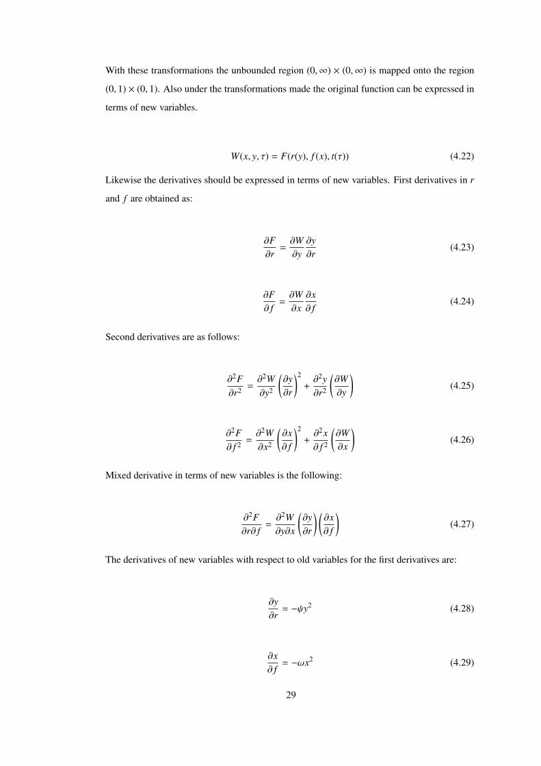
With these transformations the unbounded region (0,∞) × (0,∞) is mapped onto the region
(0, 1) × (0, 1). Also under the transformations made the original function can be expressed in
terms of new variables.
W(x, y, τ) = F(r(y), f (x), t(τ)) (4.22)
Likewise the derivatives should be expressed in terms of new variables. First derivatives in r
and f are obtained as:
∂F∂r
=∂W∂y
∂y∂r
(4.23)
∂F∂ f
=∂W∂x
∂x∂ f
(4.24)
Second derivatives are as follows:
∂2F∂r2 =
∂2W∂y2
(∂y∂r
)2
+∂2y∂r2
(∂W∂y
)(4.25)
∂2F∂ f 2 =
∂2W∂x2
(∂x∂ f
)2
+∂2x∂ f 2
(∂W∂x
)(4.26)
Mixed derivative in terms of new variables is the following:
∂2F∂r∂ f
=∂2W∂y∂x
(∂y∂r
) (∂x∂ f
)(4.27)
The derivatives of new variables with respect to old variables for the first derivatives are:
∂y∂r
= −ψy2 (4.28)
∂x∂ f
= −ωx2 (4.29)
29

The second derivatives of new variables in terms of old variables are as follows:
∂2y∂r2 = 2ψ2y3 (4.30)
∂2x∂ f 2 = 2ω2x3 (4.31)
After the substitutions the formulation for the transformed version of the PDE (3.4) is the
following:
12σ2
f f (x)ω2x4 ∂2W∂x2 + ρσrσ f
√r(y)
√f (x)ψωy2x2 ∂
2W∂x∂y
+12σ2
r r(y)ψ2y4 ∂2W∂y2 + [σ2
f f (x)ω2x3 − ωx2κ f (θ f − f (x))]∂W∂x
+[σ2r r(y)ψ2y3 − ψy2κr(θr − r(y))]
∂W∂y−∂W∂τ(t)
− r(y)W = 0
(4.32)
4.3.1.1 Consistency, Stability and Convergence of the Numerical Procedure
In numerical procedures used in this study a continuous domain is discretized along the finite
number of points. This procedure creates truncation errors for the problem and errors asso-
ciated with the problem affects the accuracy of the solution. If the errors do not grow to be
much larger, then the solution can be said to be accurate.
Following the approach used in Morton and Mayers [29] it can be said that, in order for the
numerical solution of a PDE of the type under study to converge and be stable as h, l, k → 0,
the following condition must be satisfied:
Λkh2 + Θ
kl2≤
12
(4.33)
where;
Λ = Coefficient of the second derivative term in x in equation (4.32).
Θ = Coefficient of the second derivative term in y in equation (4.32).
30
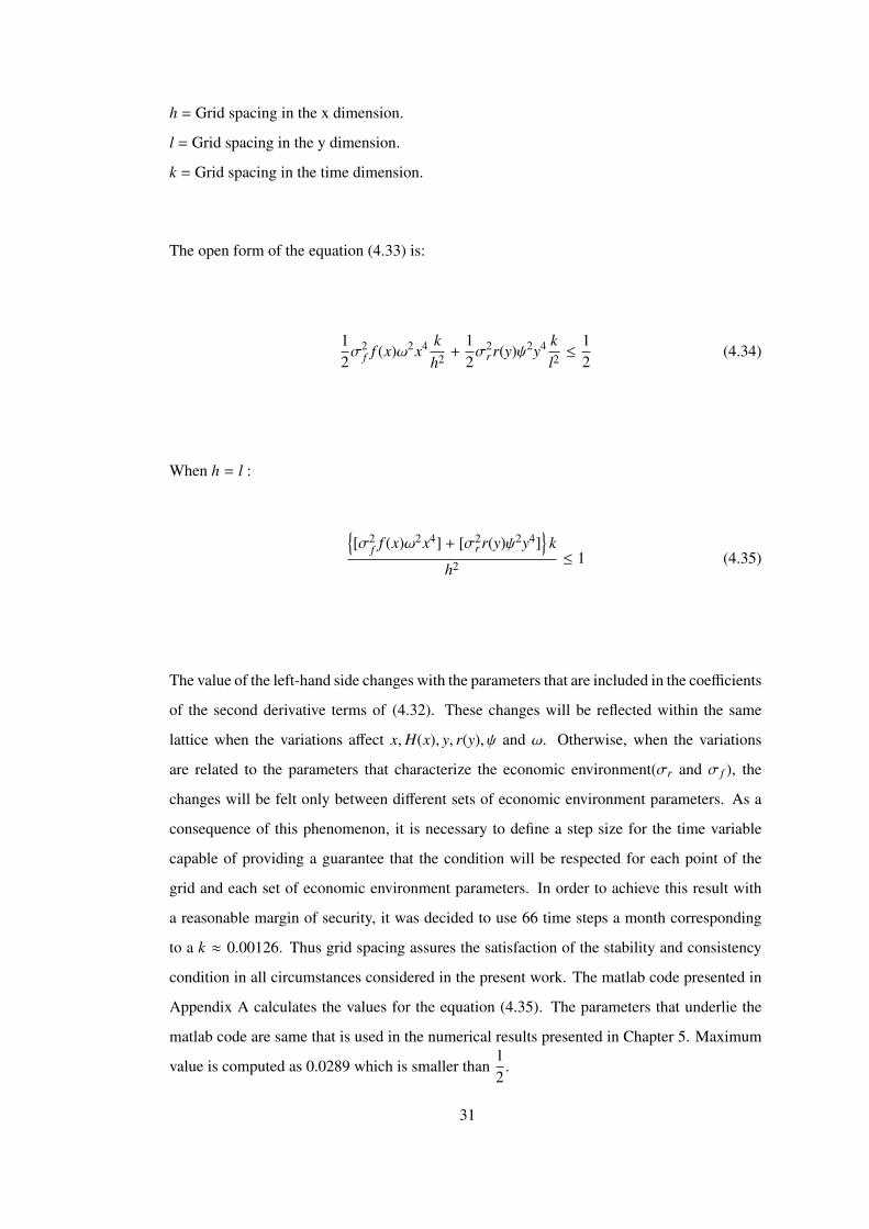
h = Grid spacing in the x dimension.
l = Grid spacing in the y dimension.
k = Grid spacing in the time dimension.
The open form of the equation (4.33) is:
12σ2
f f (x)ω2x4 kh2 +
12σ2
r r(y)ψ2y4 kl2≤
12
(4.34)
When h = l :
{[σ2
f f (x)ω2x4] + [σ2r r(y)ψ2y4]
}k
h2 ≤ 1 (4.35)
The value of the left-hand side changes with the parameters that are included in the coefficients
of the second derivative terms of (4.32). These changes will be reflected within the same
lattice when the variations affect x,H(x), y, r(y), ψ and ω. Otherwise, when the variations
are related to the parameters that characterize the economic environment(σr and σ f ), the
changes will be felt only between different sets of economic environment parameters. As a
consequence of this phenomenon, it is necessary to define a step size for the time variable
capable of providing a guarantee that the condition will be respected for each point of the
grid and each set of economic environment parameters. In order to achieve this result with
a reasonable margin of security, it was decided to use 66 time steps a month corresponding
to a k ≈ 0.00126. Thus grid spacing assures the satisfaction of the stability and consistency
condition in all circumstances considered in the present work. The matlab code presented in
Appendix A calculates the values for the equation (4.35). The parameters that underlie the
matlab code are same that is used in the numerical results presented in Chapter 5. Maximum
value is computed as 0.0289 which is smaller than12
.
31

4.3.2 Finite Difference Representation of the PDE
4.3.2.1 Interior Points
The transformed version of the PDE (4.32) can be approximated by the following difference
equation:
12σ2
f f (x)ω2x4Un
j,i+1 − 2Unj,i + Un
j,i−1
h2
+ρσrσ f√
r(y)√
f (x)ψωy2x2Un
j+1,i+1 − Unj−1,i+1 + Un
j+1,i−1 + Unj−1,i−1
4hl
+12σ2
r r(y)ψ2y4Un
j+1,i − 2Unj,i + Un
j−1,i
l2
+[σ2f f (x)ω2x3 − ωx2κ f (θ f − f (x))]
Unj,i+1 − Un
j,i−1
2h
+[σ2r r(y)ψ2y3 − ψy2κr(θr − r(y))]
Unj,i+1 − Un
j,i−1
2l
−Un+1
j,i + Unj,i
s− r(y)Un
j,i = 0
(4.36)
When the equation (4.36) rearranged, asset value at a certain time step can be found as a
function of its own value at the previous time step recursively:
Un+1j,i =
[1 − sr(y) − σ2
r r(y)ψ2y4( sl2
)− σ2
f f (x)ω2x4( sh2
)]Un
j,i
+12σ2
f f (x)ω2x4( sh2
)(Un
j,i+1 + Unj,i−1)
+12σ2
r r(y)ψ2y4( sl2
)(Un
j+1,i + Unj−1,i)
+[σ2
f f (x)ω2x3 − ωx2κ f (θ f − f (x))] ( s
2h
)(Un
j,i+1 − Unj,i−1)
+[σ2
r r(y)ψ2y3 − ψy2κr(θr − r(y))] ( s
2l
)(Un
j+1,i − Unj−1,i)
+ ρσrσ f√
r(y)√
f (x)ψωy2x2( s4hl
)(Un
j+1,i+1 − Unj−1,i+1 + Un
j+1,i−1 + Unj−1,i−1)
(4.37)
Equation (4.37) can be represented as follows when the coefficients of Unj,i’s are perfectly
isolated;
32

Un+1j,i =
[1 − sr(y) − σ2
r r(y)ψ2y4( sl2
)− σ2
f f (x)ω2x4( sh2
)]Un
j,i
+
[12σ2
f f (x)ω2x4( sh2
)+
[σ2
f f (x)ω2x3 − ωx2κ f (θ f − f (x))] ( s
2h
)]Un
j,i+1
+
[12σ2
f f (x)ω2x4( sh2
)+
[σ2
f f (x)ω2x3 − ωx2κ f (θ f − f (x))] ( s
2h
)]Un
j,i−1
+
[12σ2
r r(y)ψ2y4( sl2
)+
[σ2
r r(y)ψ2y3 − ψy2κr(θr − r(y))] ( s
2l
)]Un
j+1,i
+
[12σ2
r r(y)ψ2y4( sl2
)+
[σ2
r r(y)ψ2y3 − ψy2κr(θr − r(y))] ( s
2l
)]Un
j−1,i
+ ρσrσ f√
r(y)√
f (x)ψωy2x2( s4hl
)(Un
j+1,i+1 − Unj−1,i+1 + Un
j+1,i−1 + Unj−1,i−1)
(4.38)
The coefficients of equation (4.38) are not only the model parameters but the values are
changed across the grid by the transformed variables. In order to eliminate the stability prob-
lems and keep the errors bounded the coefficients of Un terms should be positive in equation
(4.38) [29]. Since the coefficients of the second derivative terms are always positive in equa-
tion (4.32) the coefficients of the first derivative terms must be focused on. According to
Morton & Mayers [29] this problem can be eliminated by using forward or backward differ-
ences for the first derivative instead of using central differences. The appropriate difference
method to use can be identified according to the sign of the coefficients. In this study, forward
difference approximation is used when the coefficients of the first derivative term are posi-
tive and backward difference approximation is used when the coefficient of the first derivative
term is negative. Two-dimensional PDE was used to solve the asset prices therefore there are
four combinations of first derivative signs.
4.3.2.2 Upper Boundary Conditions in the Transformed State Variables
The specifications that are made on the boundary of the domain to have a unique and well-
behaved solution for the equation are called boundary conditions. In order to simplify the
solution of the model transformed variables were used but the relevant state variables are the
original ones. Therefore, the discussion about boundary conditions should be done in terms
of the original state variables. The upper boundary conditions in the transformed variables
correspond to the lower boundary conditions in the original PDE where, f = r = 0.
All the formulation related to the boundary conditions needs to consider the degenerate ver-
33

sions of the original PDE (3.4). Transformation of the degenerate version of the PDE to the
finite difference scheme will be done by using one of the difference methods.
The Exchange Rate Dimension: When f = 0 obligation of the borrower will also be zero
when converted to domestic currency. In such a case foreign currency borrowing has no risk in
terms of exchange rate conversion. In other words exchange rate risk is eliminated. Therefore
value of all the assets will be zero and the following equations hold;
A(r, 0) = 0 (4.39)
VB(r, 0) = 0 (4.40)
D(r, 0) = 0 (4.41)
FD(r, 0) = 0 (4.42)
The Spot Interest Rate Dimension: When r = 0 there is no discounting but exchange
rate effect on the asset values still exists. Therefore, in the valuation of assets, following
degenerate form of the main PDE (3.4) will be used. It should be noted about the following
equation that although the interest rate is null there exists a first derivative in r, because this
element is not multiplied by the variable:
∂F∂t
+ κrθr∂F∂r
+ κ f (θ f − f )∂F∂ f
+12σ2
f f∂2F∂ f 2 = 0 (4.43)
4.3.2.3 Lower Boundary Conditions in the Transformed State Variables
Following the same logic stated in the previous subsection lower boundary conditions in the
transformed PDE correspond to upper boundary conditions of the original PDE. Therefore, in
this section cases in which f → ∞ and r → ∞ will be analyzed.
The Exchange Rate Dimension: When f → ∞, values of default and financial distress will
be different than 0. But both of their values depend on the value of future payments. Thus,
limf→∞
F(r, f , t) will be determined by the following degenerate PDE:
34

∂F∂t
+ κr(θr − r)∂F∂r
+ κ f θ f∂F∂ f
+12σ2
r r∂2F∂r2 − rF = 0 (4.44)
The Spot Interest Rate Dimension: When r → ∞ any future payment does not have any
value. As a result the values of all other assets are equal to zero:
limr→∞
A(r, f ) = 0 (4.45)
limr→∞
VB(r, f ) = 0 (4.46)
limr→∞
D(r, f ) = 0 (4.47)
limr→∞
FD(r, f ) = 0 (4.48)
4.3.2.4 Corners of the Grid
Both state variables can take values in the [0,∞] interval. In order to make calculations easier
those intervals are mapped to [0, 1] interval and a unit grid is obtained. Therefore corners
of the grid corresponds to points where both original state variables take the combination of
extreme values in which f = 0 or f → ∞ and r = 0 or r → ∞.
Corners in the Upper Boundary of the Transformed Interest Rate Dimension of the
Grid: In this case interest rate is null therefore there is no discounting and exchange rate
takes the extreme values f = 0 or f → ∞. When r = 0 and f = 0 the value of any asset can
be found by the following equation:
F(0, 0, t) = F(κrθr s, κ f θ f s, t + s) (4.49)
When f → ∞, the value of all assets can be found by:
limf→∞
F(0, f , t) = F(κrθr s, f , t + s) (4.50)
Corners in the Lower Boundary of the Transformed Interest Rate Dimension of the
Grid:Those are the points in which r → ∞. The value of future payments will be 0. Thus
35

the value of assets that depend on future payments will be also 0. Consequently, the values of
assets are defined by the following equations:
limr→∞
A(r, f ) = 0 (4.51)
limr→∞
VB(r, f ) = 0 (4.52)
limr→∞
D(r, f ) = 0 (4.53)
limr→∞
FD(r, f ) = 0 (4.54)
36

CHAPTER 5
ANALYSIS OF THE FOREIGN CURRENCY LOAN
VALUATION MODEL RESULTS
5.1 Introduction
Securities that are traded on stock exchanges and developed over-the-counter markets are
standardized products having common features. The parameters used in the valuation of such
products do not vary much from one product to another. On the other hand, not only foreign
currency denominated corporate loan contracts but also all types of corporate loan contracts
have specifications varying according to some features of the company. Basically, the country,
where the firm is established, sector of the business running, size of the firm and the purpose
of the credit taken affects the contract terms [45]. Parameters affecting the valuation procedure
are classified as systematic parameters and unsystematic parameters. Table 5.1 represents the
parameter values used in the construction of base case economic environment (systematic
parameters) and basic properties of the loan contract (unsystematic parameters). Sensitivities
of the asset values to the changes in these parameter values are tested along with the analysis
of financial implications of the changes.
This chapter aims to provide and discuss the numerical results provided by the model that was
presented in Chapter 3. Section 5.2 presents an overview of the valuation functions for each
of the variables under study and series of figures indicating the behavior of these functions
for different values of the state variables at the origination of the contract given. Section 5.3
develops a mathematical analysis of the effects induced by changes in the parameters that
are used to characterize the economic environment as well as the company specifications, in
terms of the valuation of the assets under study. Finally section 5.4 presents the financial
37

interpretations of the consequences induced by changes in the parameters of the contracts in
terms of the valuation functions.
5.2 Overview of the Valuation Functions
We produce 3-D figures for each of the related assets (value of loan, value of future payments,
value of default and value of financial distress) in order to show that the numerical solutions
vary across the state space smoothly, without causing any instability and that the structure of
the graphs makes sense in economic terms. Figures from 5.1 to 5.8 give a graphical image
of the value of what assumed by the valuation functions associated with the contract specifi-
cations under study along the state space at the contract origination. Each presented figure is
produced based on the (36×45) dimensional grid located in the economically reasonable part
of the corresponding grid with dimensions (51× 51). According to the (36× 45) dimensional
grid interest rate and exchange rate are in the intervals [0.0020, 0.9000] and [0.0305, 3.8380]
respectively.
Figures 5.1 and 5.2 present the variable A for initial leverage ratios of 80% and 90% re-
spectively. The resulting figure verifies the expectations for both interest rate dimension and
exchange rate dimension. It is seen that value of future payments, being independent of the
initial capital structure of the firm, is inversely related with the interest rate and in direct
relationship with the exchange rate.
Value of the loan, V , is a function of A and D. High exchange rates triggers the event of
default and increase the value of default, D. In the regions where default has positive value,
V stabilizes in the value equal to total assets of the firm (Figure 5.3, Figure 5.4). Revealing
the fact that in the event of default firm can pay as much as its assets independent of exchange
rate increase. The effect of initial foreign currency denominated loan to total assets ratio alters
the nodes where the value stabilization begins. Examining the value of the contract in terms
of state variables, it is seen that until default occurs, the relations between the contract value,
interest rate and exchange rate are influenced by A.
Value of the default option, D, is exhibited in Figure 5.5 and Figure 5.6. It is derived from
the figures that default tends to occur in the region where interest rates are low and exchange
38

rates are high. For the interest rate dimension, our findings are consistent with the claims on
Moody’s analytics report [34], which states that if the economy is in recession and the default
rate is high, interest rates are often relatively low due to the traditional central bank monetary
policy of lowering rates in order to awaken the economy. When the economy improves, the
central bank tends to raise the rates, correspondingly.
Since an increase in interest rate (discount rate) decreases the value of both A and V , the
dominant state variable affecting the value of D is exchange rate. Moreover, the default region
changes according to the initial LTV ratios. With higher initial LTV ratios default occurs for
the lower values of exchange rate compared to lower LTV ratios at the origination of the
contract.
Finally, Figure 5.7 and 5.8 show the value of financial distress, FD, for the different values of
state variables. FD has similar characteristics with the implicit put option, but it gets positive
values when the value of future payments exceeds the distress threshold. Therefore, even
in low exchange rates, financial distress is a problem for the firm due to foreign currency
denominated loan. In the interest rate dimension, being related with A, value of FD decreases
with the increase of interest rate.
5.3 Mathematical Interpretations of the Model
As noted earlier in the introduction section, the economic environment is described by the
parameters given in Table 5.1. The exchange rate data required for this study is gathered from
the Central Bank of the Republic of Turkey and the exchange rate parameters are estimated
by employing Maximum Likelihood Estimation method. Interest rate parameters are taken
from the study of Erol [44]. In this section effects of changes in the parameter values on the
numeric solutions of the asset values will be analyzed.
5.3.1 Interest Rate Volatility
In Chapter 3 all the assets under study are modeled as a function of interest rate. Therefore,
fluctuations in interest rate affect all the assets. Table 5.3 and 5.4 shows the sensitivities of the
39

foreign currency denominated loan contract and related assets’ values to changes in interest
rate volatility, σr for different exchange rates.
Value of future payments, which affects the values of all the assets under study, increases as
the volatility of interest rate increase. In other words, high and low levels of discount rate
arising from an increment in σr leads to an increase in the value of A. Rising discount rates
decrease the present value of expected cash-flows whereas decline in interest rates increase
its value. Nevertheless, the downward changes in interest rates have more influence on the
present value of expected cash-flows than upward changes in the same degree, which can
be explained by the Jensen’s inequality. Jensen’s inequality states that expected value of a
convex function of a random variable is greater than the convex function of an expectation of
a random variable.
The values of default and financial distress are affected by the value of the future payments.
As the volatility of interest rate and the value of future payments increase, values of D and
FD also increase.
Interest rate volatility and the value of the contract have an inverse relationship. This is an
unexpected result since the equation (3.8) holds and both the value of the future payments and
the value of default have direct relationship with the volatility of interest rate. However, an
increment in σr influences the value of D more than it affects the value of A.
5.3.2 Exchange Rate Volatility
Impact of changes in exchange rate volatility on the assets under study has some different
characteristics with the impact of interest rate volatility. Also, exchange rate and interest
rate increases and decreases affect the asset values in the model in a different way. When
the interest rate increases the values of all the assets decrease whereas when exchange rate
increases the value of all the assets also increase (see Table 5.5 and Table 5.6).
For the high levels of exchange rate volatility, σ f , the value of future payments increases but
for the low levels of σ f the increase in the value of A can not be sustained. According to
our numerical results, continuous increase in the value of expected payoffs occurs when the
volatility of exchange rate takes values higher than 0.30.
40

Value of financial distress shows similar characteristic with the value of A. In chapter 3 it is
stated that if the value of future payments, A, surpasses a certain predefined distress barrier
then this situation induces financial distress for the firm. Therefore, value of FD having direct
relationship with the value of A increases as the volatility of exchange rate increases to high
levels. Although value of the default option, D, is also in direct relation with A, being in
inverse relation with the value of the contract, V , keeps its value to increase continuously as
σ f increases. Value of the loan decreases as the exchange rate volatility increases due to the
equation (3.8) given in chapter 3 since the changes in default value is greater than the changes
in the value of future payments for the same amount of increase in σ f .
5.3.3 Correlation Between Wiener Processes
In Table 5.7 and Table 5.8 numerical results influenced with the change in correlation coeffi-
cient between Wiener processes, ρ, are presented. Tables show that as ρ increases, the value
of the assets decrease, which implies inverse relation between r and f . In other words, for the
high values of r default does not tend to occur since increasing discount rate reduces the value
of A. However, when r is low and f is high default is more likely to happen. As a consequence
these factors creates a tendency for the value of default to evolve in inverse relationship with
ρ. Change in state variables affect the value of future payments in the opposite direction and
all the assets valued in this study have direct relationship with the value of A. Therefore, it is
an expected result to have negative relation between the correlation coefficient and the values
of the assets.
5.3.4 Initial Loan to Value Ratio
Tables 5.9 to 5.12 represents the value of assets (V, A,D, FD) for different levels of loan
to value ratios and for different levels of exchange rates, f = 1.8996, f = 2.2388, f =
2.6534 and f = 3.1716. Recent developments show that Turkish lira considerably loses
value, devaluates against dollar, euro and pound. According to recent exchange rate levels,
f = 1.8996 can be thought as Turkish lira to dollar, f = 2.2388 and f = 2.6534 as Turkish lira
to euro, finally f = 3.1716 can be thought as turkish lira to pound exchange rates. Empirical
data shows that for utilities sector average FX-loan to total asset ratio was nearly 55% in
41

2009, when we began this study. Therefore, we tested different levels of LTV ratios between
55% − 100%.
LTV ratio is used to determine the amount of the loan. Therefore, for higher LTV ratios value
of A will be higher. As LTV ratio gets closer to 1, the conditions for the value of A to pass
the value of total assets of the firm is created. Following with the event of default defined in
chapter 3 tends to occur. For the higher values of LTV ratios and exchange rates the value of
the loan stays bounded by the value of the assets of the firm. Also for higher levels of these
parameters default and financial distress have significantly higher values.
5.3.5 Financial Distress Barrier
Threshold value for foreign currency loans to total assets ratio indicates the financial distress
barrier for the firm. According to model and valuation functions constructed in Chapter 3, it
is expected to see the effect of changing the threshold only on the value of Financial Distress.
Hence, the numeric results presented in Table 5.13 are anticipated results. Also from Table
5.14 it can be seen that the effect of increasing threshold values by 0.05 on the value of
FD is in the same amount with the increment for different LTV-ratios. Those two tables are
presented to show that our model works correctly.
5.4 Financial Implications of the Model
The main aim of this study is to identify the behaviors of default and financial distress in for-
eign currency denominated loans of non-financial firms according to their capital structure.
Financial leverage is defined as the ratio of total liabilities to total assets of the firm. It is gen-
erally accepted that when this ratio gets closer to one then it is said that the firm is in financial
distress, which is a signal to default for the firm. It is expected to observe the effects of foreign
borrowing in firms whose borrowings are mostly in foreign currency. Most specifically, in or-
der to identify the financial distress induced by foreign currency denominated loans clearly,
that is to say to eliminate the other effects causing financial distress as much as possible, we
focused on the sectors whose foreign currency denominated loan to total loans ratio is high.
It is also expected that for such firms, effects of fluctuations in exchange rates on the capital
42

structure of the firm can be seen directly. Following these arguments parameters presented in
Table 5.1 are determined.
The firms in Electricity, Gas and Water Sources, or the utilities sector whose stocks are traded
in ISE100 have the highest foreign currency denominated loan to total loans ratio that is 93%,
among other sectors. Tourism is the second sector with the ratio of 78% and Metal Industries
is the third sector with the ratio of 70% according to this listing [4]. The historical, quarterly
financial statements of the firms in these sectors are obtained from Istanbul Stock Exchange
website. From notes to financial statements foreign currency denominated loan composition
of the firms are obtained and currency loan to total assets ratio is calculated for the period
2001 to 2009. The effect of foreign borrowing can differ according to size of the company.
We classified the utilities sector firms as ”big” and ”small” considering their total asset values.
Having classified the companies according to their asset values we identified distress barriers
for these firms following the work of Opler & Titman [26]. The authors defined the firms
having debt to asset ratio in deciles 8 to 10 as being highly leveraged. Our data shows that for
the firms with higher asset values, total debt to asset ratio equals to 60% in decile 8. Therefore,
it is reasonable to assume that when the foreign currency loan to total asset ratio exceeds the
sector’s total debt to total asset ratio in decile 8 there occurs a financial distress for the firm.
Based on this assumption we set the distress barrier as 60% for companies with total asset
value greater than 600M TL in energy sector. Table 5.2 shows the table of leverage ratios to
relative deciles for those firms.
Firms that mostly rely on debt financing and having high volumes of foreign currency denom-
inated loans raised their fx-borrowing to total asset ratios up to 80% between the years 2001
and 2009. In the light of these findings we took 80% as the base value for loan-to-value (LTV)
ratio. However, we test the different compositions of foreign currency denominated loans to
total assets ratio and identified the distress percentages for respective ratios.
Disclosed notes to financial statements show that the maturity of foreign currency loans clus-
tered up to five years. Also, foreign borrowings are mostly denominated in dollar. Hence we
choose the maturity of the loan as 60 months and initial exchange rate as 1.523 FX/TL for
calculations used in MATLAB code (see Appendix B).
43
5.4.1 Effect of LTV Ratio
In this model LTV ratio identifies the initial loan amount as a domestic-currency loan. All
asset values are in domestic currency and indicate the ratio of the valued asset to total assets
of the firm. Specifically, when exchange rate is 2.6534 times the domestic currency and LTV
ratio is 80%, the value of financial distress due to foreign currency denominated loan is 50%
of the total assets of the firm, value of the default is 11% of the total assets of the firm, value
of the remaining payments of the firm and the value of the currency loan is 110% and 99% in
terms of the total assets of the firm, respectively (see Table 5.11).
In tables 5.9 to 5.12 it is seen that as the borrowing in foreign currency increases, the value
of FD and D increase to levels that cannot be neglected. For lower exchange rate values, the
value of financial distress reaches to 40% levels and the value of default stays in manageable
levels. As exchange rate increases, the value of FD increases significantly and the value of
D does not stay in manageable levels. Moreover, for higher values of exchange rates, value
of FD is considerably high even for the LTV ratios around the distress barrier (see Tables
5.11 and 5.12). Default gets non-zero values for even low LTV ratios as FX-rate increases.
However, for small values of D we cannot jump into conclusion that the firm experiences
default. In reality, default event occurs only if corporations are borrowing very high LTV
loans with considerably high FX-rates.
5.4.2 Effect of Volatilities
The valuation functions of the derivative assets are constructed considering the main risk
factors. Fluctuations in exchange rate and interest rate are determined as the main factors
affecting the values of the financial distress and the default. The variations of state variables
are included to model with the parameters σ f and σr. The analysis of sensitivities of the
numerical results to change in volatility values is presented in the previous section and it is
stated that both of the volatilities of the state variables are in direct relationship with the values
of FD and D.
In tables 5.4 and 5.6, standalone effects of changes in the volatilities of interest rate and
exchange rate on asset values are presented, respectively. Our results reveal that interest rate
44

volatility is reasonably more effective on financial distress and default risks in comparison to
exchange rate volatility. In detail, change in interest rate volatility by 0.03 changes the distress
value and the default value higher compared to 0.03 change in exchange rate volatility does.
On the other hand, it should be noted that the numerical results show that up to certain level
of increase in σr the value of the assets increase. After that certain level, which is nearly
0.39 in this model, increase in interest rate volatility decreases the value of the assets sharper
than while it is increasing. However, it is very unlikely for interest rate volatility to reach that
levels. Furthermore, as exchange rate volatility takes high values, increase in the value of FD
can be seen clearly. However, still for those levels of exchange rate volatility, the effect of σ f
on FD values is less than the effect of change in σr.
In summary, the effect of fluctuations of discount rate on the value of financial distress is
dominant compared to the effect of variances in exchange rate. This result can be interpreted
in two ways. First, since exchange rate and interest rate have inverse relation with each other
when the variance for interest rate is in negative direction, the variance in exchange rate is
expected to be in positive direction. Both of them are the cases that increase the value of
financial distress. Moreover, increment in exchange rate increases the value of FD sharper
than the decrease in r.On the other hand, for the lower values of exchange rate FD has no
value. Although increase in exchange rate increases the value of FD sharper than the decrease
in r, for exchange rate movements in opposite direction, for lower exchange rates FD has no
value. In total, the effect of exchange rate volatility on the value of financial distress will be
less compared to the effect of interest rate volatility. Second, if we consider the volatility in
terms of upside risk in exchange rate dimension we see that the effect of a rise in exchange
rate on the value of FD is sharper than a decrease in the value of r. In Turkey, we commonly
observe upward movements in the exchange rate. Considering the exchange rate trends in
Turkey and our results, which reveal the importance of the currency devaluation risk for FX-
borrowing, we identify the exchange rate increase as the main risk factor for corporations that
are heavily financed by FX-loans.
If volatility in interest rates leads to higher interest rates in the market, as commonly observed
in Turkey, mathematically the present value of credit payments will be lower due to a higher
discount factor. Correspondingly, lower payments will not result in financial distress for the
corporations. Besides, higher interest rates should be explained as the higher opportunity cost
of capital from financial perspective. As the cost of borrowing in domestic currency increases
45

(high interest rates), we would expect to see lower financial distress for corporations that are
heavily financed by FX-loans. Furthermore, as the cost of borrowing in foreign currency is
lower than the domestic currency borrowing, in such an environment firms tend to issue more
FX-loans. Turkish economy experienced that case after 2001 when the cost of borrowing in
domestic currency was high firms started to issue more FX-loan, which led to higher FX-loan
to total asset ratios for the firms.
Overall, our results demonstrate that corporations that are heavily financed by FX-loans can
easily experience financial distress under volatile economies like Turkey. We argue that under
the volatile financial environment of Turkey, utilities sector has experienced financial distress
as long as TL devaluates against US dollar and euro. In this study calculations are made
based on the assumption that FX-loan positions of the firms are unhedged and asset value of
the firm is constant. In that respect, the values of FD and D can be defined as the amounts
of hedged positions, that firms should have in their capital structure to avoid financial distress
and default, in terms of total assets value of the firms. Moreover, in financial perspective,
the default event occurs only if corporations are borrowing very high LTV loans (like 95% −
100%) with considerably high exchange rates when volatility of interest rate is high. In detail,
Table 5.10 shows that for the exchange rate (FX-rate) of 2.2388, 100% LTV loans result in
a significant default value of 21% of the total asset value of the firm. Table 5.11 shows that
for the FX-rate of 2.6534, not only 100% LTV loans but also 95% LTV loans result in default
values of 38.5% and 31.6% of total asset value of the firm, respectively. Finally, the default is
likely to occur with 85%− 100% LTV loans when FX-rate is at the 3.1716 level. Under these
circumstances, the value of default reaches up to 36% to 60% of asset value of the firm.
46

Figu
re5.
1:V
alue
ofFu
ture
Paym
ents
(A)(
LTV
=0.
80)
00.
20.
40.
60.
81
0
1
2
3
40
0.51
1.52
r (I
nter
est R
ate)
Val
ue o
f Fut
ure
Pay
men
ts (
LTV
=80
%)
f (E
xcha
nge
Rat
e)
A (Future Payments)
The
follo
win
gpa
ram
eter
sw
ere
used
inth
eco
nstr
uctio
nof
this
figur
e:th
esp
otin
tere
stra
ter
is10
%,t
heex
chan
gera
tef in
tis
1.52
30,l
ong-
term
mea
n
reve
rsio
nra
teof
inte
rest
rateκ r
is0.
56,l
ong-
term
mea
nre
vers
ion
rate
ofex
chan
gera
teκ
fis
0.15
,lon
gte
rmm
ean
ofin
tere
stra
teθ r
is0.
24,l
ong
term
mea
nof
exch
ange
rateθ
fis
1.86
,the
inte
rest
rate
vola
tility
σr
is0.
12,t
heex
chan
gera
tevo
latil
ityσ
fis
0.21
,fina
ncia
ldis
tres
sth
resh
old
is0.
60,L
TV
ratio
is0.
80,t
heco
rrel
atio
nco
effici
entρ
is0
47

Figu
re5.
2:V
alue
ofFu
ture
Paym
ents
(A)(
LTV
=0.
90)
00.
20.
40.
60.
81
0
1
2
3
40
0.51
1.52
r (I
nter
est R
ate)
Val
ue o
f Fut
ure
Pay
men
ts (
LTV
=90
%)
f (E
xcha
nge
Rat
e)
A (Future Payments)
The
follo
win
gpa
ram
eter
sw
ere
used
inth
eco
nstr
uctio
nof
this
figur
e:th
esp
otin
tere
stra
ter
is10
%,t
heex
chan
gera
tef in
tis
1.52
30,l
ong-
term
mea
n
reve
rsio
nra
teof
inte
rest
rateκ r
is0.
56,l
ong-
term
mea
nre
vers
ion
rate
ofex
chan
gera
teκ
fis
0.15
,lon
gte
rmm
ean
ofin
tere
stra
teθ r
is0.
24,l
ong
term
mea
nof
exch
ange
rateθ
fis
1.86
,the
inte
rest
rate
vola
tility
σr
is0.
12,t
heex
chan
gera
tevo
latil
ityσ
fis
0.21
,fina
ncia
ldis
tres
sth
resh
old
is0.
60,L
TV
ratio
is0.
90,t
heco
rrel
atio
nco
effici
entρ
is0
48

Figu
re5.
3:V
alue
ofL
oan
(V)(
LTV
=0.
80)
00.
20.
40.
60.
81
0
1
2
3
40
0.2
0.4
0.6
0.81
r (I
nter
est R
ate)
Val
ue o
f the
Loa
n (L
TV
=80
%)
f (E
xcha
nge
Rat
e)
V (Value of the Loan)
The
follo
win
gpa
ram
eter
sw
ere
used
inth
eco
nstr
uctio
nof
this
figur
e:th
esp
otin
tere
stra
ter
is10
%,t
heex
chan
gera
tef in
tis
1.52
30,l
ong-
term
mea
n
reve
rsio
nra
teof
inte
rest
rateκ r
is0.
56,l
ong-
term
mea
nre
vers
ion
rate
ofex
chan
gera
teκ
fis
0.15
,lon
gte
rmm
ean
ofin
tere
stra
teθ r
is0.
24,l
ong
term
mea
nof
exch
ange
rateθ
fis
1.86
,the
inte
rest
rate
vola
tility
σr
is0.
12,t
heex
chan
gera
tevo
latil
ityσ
fis
0.21
,fina
ncia
ldis
tres
sth
resh
old
is0.
60,L
TV
ratio
is0.
80,t
heco
rrel
atio
nco
effici
entρ
is0
49

Figu
re5.
4:V
alue
ofL
oan
(V)(
LTV
=0.
90)
00.
20.
40.
60.
81
0
1
2
3
40
0.2
0.4
0.6
0.81
r (I
nter
est R
ate)
Val
ue o
f the
Loa
n (L
TV
=90
%)
f (E
xcha
nge
Rat
e)
V (Value of the Loan)
The
follo
win
gpa
ram
eter
sw
ere
used
inth
eco
nstr
uctio
nof
this
figur
e:th
esp
otin
tere
stra
ter
is10
%,t
heex
chan
gera
tef in
tis
1.52
30,l
ong-
term
mea
n
reve
rsio
nra
teof
inte
rest
rateκ r
is0.
56,l
ong-
term
mea
nre
vers
ion
rate
ofex
chan
gera
teκ
fis
0.15
,lon
gte
rmm
ean
ofin
tere
stra
teθ r
is0.
24,l
ong
term
mea
nof
exch
ange
rateθ
fis
1.86
,the
inte
rest
rate
vola
tility
σr
is0.
12,t
heex
chan
gera
tevo
latil
ityσ
fis
0.21
,fina
ncia
ldis
tres
sth
resh
old
is0.
60,L
TV
ratio
is0.
90,t
heco
rrel
atio
nco
effici
entρ
is0
50

Figu
re5.
5:V
alue
ofFi
nanc
ialD
istr
ess
(FD
)(LT
V=
0.80
)
00.
20.
40.
60.
81
0
1
2
3
40
0.2
0.4
0.6
0.81
1.2
r (I
nter
est R
ate)
Val
ue o
f Fin
anci
al D
istr
ess
(LT
V=
80%
)
f (E
xcha
nge
Rat
e)
FD (Financial Distress)
The
follo
win
gpa
ram
eter
sw
ere
used
inth
eco
nstr
uctio
nof
this
figur
e:th
esp
otin
tere
stra
ter
is10
%,t
heex
chan
gera
tef in
tis
1.52
30,l
ong-
term
mea
n
reve
rsio
nra
teof
inte
rest
rateκ r
is0.
56,l
ong-
term
mea
nre
vers
ion
rate
ofex
chan
gera
teκ
fis
0.15
,lon
gte
rmm
ean
ofin
tere
stra
teθ r
is0.
24,l
ong
term
mea
nof
exch
ange
rateθ
fis
1.86
,the
inte
rest
rate
vola
tility
σr
is0.
12,t
heex
chan
gera
tevo
latil
ityσ
fis
0.21
,fina
ncia
ldis
tres
sth
resh
old
is0.
60,L
TV
ratio
is0.
80,t
heco
rrel
atio
nco
effici
entρ
is0
51

Figu
re5.
6:V
alue
ofFi
nanc
ialD
istr
ess
(FD
)(LT
V=
0.90
)
00.
20.
40.
60.
81
0
1
2
3
40
0.2
0.4
0.6
0.81
1.2
r (I
nter
est R
ate)
Val
ue o
f Fin
anci
al D
istr
ess
(LT
V=
90%
)
f (E
xcha
nge
Rat
e)
FD (Financial Distress)
The
follo
win
gpa
ram
eter
sw
ere
used
inth
eco
nstr
uctio
nof
this
figur
e:th
esp
otin
tere
stra
ter
is10
%,t
heex
chan
gera
tef in
tis
1.52
30,l
ong-
term
mea
n
reve
rsio
nra
teof
inte
rest
rateκ r
is0.
56,l
ong-
term
mea
nre
vers
ion
rate
ofex
chan
gera
teκ
fis
0.15
,lon
gte
rmm
ean
ofin
tere
stra
teθ r
is0.
24,l
ong
term
mea
nof
exch
ange
rateθ
fis
1.86
,the
inte
rest
rate
vola
tility
σr
is0.
12,t
heex
chan
gera
tevo
latil
ityσ
fis
0.21
,fina
ncia
ldis
tres
sth
resh
old
is0.
60,L
TV
ratio
is0.
90,t
heco
rrel
atio
nco
effici
entρ
is0
52

Figu
re5.
7:V
alue
ofD
efau
lt(D
)(LT
V=
0.80
)
00.
20.
40.
60.
81
0
1
2
3
40
0.1
0.2
0.3
0.4
0.5
0.6
r (I
nter
est R
ate)
Val
ue o
f Def
ault
(LT
V=
80%
)
f (E
xcha
nge
Rat
e)
D (Default Option)
The
follo
win
gpa
ram
eter
sw
ere
used
inth
eco
nstr
uctio
nof
this
figur
e:th
esp
otin
tere
stra
ter
is10
%,t
heex
chan
gera
tef in
tis
1.52
30,l
ong-
term
mea
n
reve
rsio
nra
teof
inte
rest
rateκ r
is0.
56,l
ong-
term
mea
nre
vers
ion
rate
ofex
chan
gera
teκ
fis
0.15
,lon
gte
rmm
ean
ofin
tere
stra
teθ r
is0.
24,l
ong
term
mea
nof
exch
ange
rateθ
fis
1.86
,the
inte
rest
rate
vola
tility
σr
is0.
12,t
heex
chan
gera
tevo
latil
ityσ
fis
0.21
,fina
ncia
ldis
tres
sth
resh
old
is0.
60,L
TV
ratio
is0.
80,t
heco
rrel
atio
nco
effici
entρ
is0
53

Figu
re5.
8:V
alue
ofD
efau
lt(D
)(LT
V=
0.90
)
00.
20.
40.
60.
81
0
1
2
3
40
0.2
0.4
0.6
0.81
r (I
nter
est R
ate)
Val
ue o
f Def
ault
(LT
V=
90%
)
f (E
xcha
nge
Rat
e)
D (Default Option)
The
follo
win
gpa
ram
eter
sw
ere
used
inth
eco
nstr
uctio
nof
this
figur
e:th
esp
otin
tere
stra
ter
is10
%,t
heex
chan
gera
tef in
tis
1.52
30,l
ong-
term
mea
n
reve
rsio
nra
teof
inte
rest
rateκ r
is0.
56,l
ong-
term
mea
nre
vers
ion
rate
ofex
chan
gera
teκ
fis
0.15
,lon
gte
rmm
ean
ofin
tere
stra
teθ r
is0.
24,l
ong
term
mea
nof
exch
ange
rateθ
fis
1.86
,the
inte
rest
rate
vola
tility
σr
is0.
12,t
heex
chan
gera
tevo
latil
ityσ
fis
0.21
,fina
ncia
ldis
tres
sth
resh
old
is0.
60,L
TV
ratio
is0.
90,t
heco
rrel
atio
nco
effici
entρ
is0
54

Tabl
e5.
1:B
ase
Val
ues
PAR
AM
ET
ER
S
Syst
emat
icPa
ram
eter
sU
nsys
tem
atic
Para
met
ers
Spot
Inte
rest
Rat
e,r(
0)10
%M
atur
ityη
60m
onth
s
Lon
g-te
rmm
ean
reve
rsio
nra
teof
inte
rest
rateκ r
0.56
Initi
allo
anto
valu
era
tio0.
80
long
term
mea
nof
inte
rest
rateθ r
0.24
Fina
ncia
lDis
tres
sT
hres
hold
0.60
Inte
rest
rate
vola
tility
σr
0.12
Initi
alex
chan
gera
tef in
t1.
5230
$/T
L
long
-ter
mm
ean
reve
rsio
nra
teof
exch
ange
rateκ
f0.
15
long
term
mea
nof
exch
ange
rateθ
f1.
86
exch
ange
rate
vola
tility
σf
0.21
Cor
rela
tion
coeffi
cien
tρ0
55

Tabl
e5.
2:To
talL
iabi
litie
sto
Tota
lAss
ets
Rat
io
Dec
ileV
A≥
600
MT
LV
A≤
600
MT
L
0.1
22%
53%
0.2
27%
54%
0.3
31%
56%
0.4
35%
60%
0.5
38%
62%
0.6
42%
63%
0.7
46%
67%
0.8
60%
71%
0.9
76%
73%
110
5%77
%
Abo
vera
tios
repr
esen
tsth
ele
vera
gera
tios
ofth
efir
ms
inen
ergy
sect
ortr
aded
atIS
Efo
rthe
peri
odbe
twee
n20
01an
d20
09
56

Tabl
e5.
3:C
hang
esin
Vola
tility
ofIn
tere
stR
ate
(f=
1.89
96)
Vola
tility
Fina
ncia
lDis
tres
sD
efau
ltFu
ture
Paym
ents
Loa
n
σr
FDD
AV
0.03
0.24
260.
0003
0.83
730.
8369
0.06
0.24
320.
0004
0.83
790.
8368
0.09
0.24
790.
0005
0.84
260.
8365
0.12
0.25
180.
0007
0.84
640.
8361
0.15
0.25
620.
0009
0.85
080.
8354
0.18
0.26
990.
0019
0.86
450.
8343
0.21
0.28
670.
0043
0.88
110.
8328
0.24
0.30
500.
0090
0.89
940.
8309
0.27
0.32
350.
0170
0.91
790.
8283
0.30
0.34
130.
0343
0.93
570.
8249
0.33
0.35
690.
0520
0.95
170.
8204
0.36
0.37
970.
0751
0.97
570.
8142
0.39
0.38
290.
0824
0.97
960.
8054
The
follo
win
gpa
ram
eter
sw
ere
used
inth
eco
nstr
uctio
nof
this
tabl
e:th
esp
otin
tere
stra
ter
is10
%,
the
exch
ange
rate
fis
1.89
96,
long
-ter
mm
ean
reve
rsio
nra
teof
inte
rest
rateκ r
is0.
56,l
ong-
term
mea
nre
vers
ion
rate
ofex
chan
gera
teκ
fis
0.15
,lon
gte
rmm
ean
ofin
tere
stra
teθ r
is0.
24,l
ong
term
mea
nof
exch
ange
rateθ
fis
1.86
,the
exch
ange
rate
vola
tility
σf
is0.
21,fi
nanc
iald
istr
ess
thre
shol
dis
0.60
,LT
Vra
tiois
0.80
,the
corr
elat
ion
coeffi
cien
t
ρis
0
57

Tabl
e5.
4:C
hang
esin
Vola
tility
ofIn
tere
stR
ate
(f=
2.23
88)
Vola
tility
Fina
ncia
lDis
tres
sD
efau
ltFu
ture
Paym
ents
Loa
n
σr
FDD
AV
0.03
0.35
490.
0066
0.94
960.
9429
0.06
0.35
560.
0069
0.95
020.
9426
0.09
0.36
170.
0091
0.95
630.
9421
0.12
0.36
650.
0112
0.96
110.
9412
0.15
0.37
210.
0142
0.96
670.
9401
0.18
0.38
940.
0271
0.98
390.
9384
0.21
0.41
020.
0585
1.00
470.
9364
0.24
0.43
260.
0858
1.02
700.
9337
0.27
0.45
500.
1111
1.04
930.
9304
0.30
0.47
600.
1427
1.07
050.
9263
0.33
0.49
440.
1662
1.08
920.
9212
0.36
0.52
150.
1998
1.11
750.
9144
0.39
0.52
570.
2128
1.12
240.
9053
The
follo
win
gpa
ram
eter
sw
ere
used
inth
eco
nstr
uctio
nof
this
tabl
e:th
esp
otin
tere
stra
ter
is10
%,
the
exch
ange
rate
fis
2.23
88,
long
-ter
mm
ean
reve
rsio
nra
teof
inte
rest
rateκ r
is0.
56,l
ong-
term
mea
nre
vers
ion
rate
ofex
chan
gera
teκ
fis
0.15
,lon
gte
rmm
ean
ofin
tere
stra
teθ r
is0.
24,l
ong
term
mea
nof
exch
ange
rateθ
fis
1.86
,the
exch
ange
rate
vola
tility
σf
is0.
21,fi
nanc
iald
istr
ess
thre
shol
dis
0.60
,LT
Vra
tiois
0.80
,the
corr
elat
ion
coeffi
cien
t
ρis
0
58

Tabl
e5.
5:C
hang
esin
Vola
tility
ofE
xcha
nge
Rat
e(f
=1.
8996
)
Vola
tility
Fina
ncia
lDis
tres
sD
efau
ltFu
ture
Paym
ents
Loa
n
σf
FDD
AV
0.03
0.25
250
0.84
720.
8360
0.06
0.25
140
0.84
610.
8361
0.09
0.25
060
0.84
530.
8362
0.12
0.25
020
0.84
480.
8363
0.15
0.25
000.
0001
0.84
460.
8363
0.18
0.25
200.
0003
0.84
660.
8362
0.21
0.25
180.
0007
0.84
640.
8361
0.24
0.25
160.
0014
0.84
620.
8357
0.27
0.25
260.
0025
0.84
720.
8349
0.30
0.25
250.
0040
0.84
710.
8339
0.33
0.25
240.
0060
0.84
700.
8324
0.36
0.25
320.
0086
0.84
780.
8305
0.39
0.25
370.
0115
0.84
830.
8283
The
follo
win
gpa
ram
eter
sw
ere
used
inth
eco
nstr
uctio
nof
this
tabl
e:th
esp
otin
tere
stra
ter
is10
%,
the
exch
ange
rate
fis
1.89
96,
long
-ter
mm
ean
reve
rsio
nra
teof
inte
rest
rateκ r
is0.
56,l
ong-
term
mea
nre
vers
ion
rate
ofex
chan
gera
teκ
fis
0.15
,lon
gte
rmm
ean
ofin
tere
stra
teθ r
is0.
24,l
ong
term
mea
nof
exch
ange
rateθ
fis
1.86
,the
inte
rest
rate
vola
tility
σr
is0.
12,fi
nanc
iald
istr
ess
thre
shol
dis
0.60
,LT
Vra
tiois
0.80
,the
corr
elat
ion
coeffi
cien
tρ
is0
59

Tabl
e5.
6:C
hang
esin
Vola
tility
ofE
xcha
nge
Rat
e(f
=2.
2388
)
Vola
tility
Fina
ncia
lDis
tres
sD
efau
ltFu
ture
Paym
ents
Loa
n
σf
FDD
AV
0.03
0.36
720.
0003
0.96
180.
9478
0.06
0.36
700.
0009
0.96
170.
9475
0.09
0.36
670.
0021
0.96
130.
9470
0.12
0.36
630.
0036
0.96
090.
9461
0.15
0.36
590.
0057
0.96
050.
9449
0.18
0.36
670.
0083
0.96
130.
9433
0.21
0.36
650.
0112
0.96
110.
9412
0.24
0.36
630.
0146
0.96
100.
9388
0.27
0.36
700.
0185
0.96
160.
9358
0.30
0.36
690.
0226
0.96
150.
9324
0.33
0.36
690.
0271
0.96
150.
9287
0.36
0.36
740.
0320
0.96
200.
9246
0.39
0.36
790.
0371
0.96
250.
9203
The
follo
win
gpa
ram
eter
sw
ere
used
inth
eco
nstr
uctio
nof
this
tabl
e:th
esp
otin
tere
stra
ter
is10
%,
the
exch
ange
rate
fis
2.23
88,
long
-ter
mm
ean
reve
rsio
nra
teof
inte
rest
rateκ r
is0.
56,l
ong-
term
mea
nre
vers
ion
rate
ofex
chan
gera
teκ
fis
0.15
,lon
gte
rmm
ean
ofin
tere
stra
teθ r
is0.
24,l
ong
term
mea
nof
exch
ange
rateθ
fis
1.86
,the
inte
rest
rate
vola
tility
σr
is0.
12,fi
nanc
iald
istr
ess
thre
shol
dis
0.60
,LT
Vra
tiois
0.80
,the
corr
elat
ion
coeffi
cien
tρ
is0
60

Tabl
e5.
7:C
hang
esin
Cor
rela
tion
Coe
ffici
ent(
f=
1.89
96)
Cor
rela
tion
Fina
ncia
lDis
tres
sD
efau
ltFu
ture
Paym
ents
Loa
n
ρFD
DA
V
-0.2
00.
2523
0.00
090.
847
0.83
76
-0.1
50.
2522
0.00
080.
8468
0.83
72
-0.1
00.
2521
0.00
080.
8467
0.83
68
-0.0
50.
2519
0.00
070.
8465
0.83
65
0.00
0.25
180.
0007
0.84
640.
8361
0.05
0.25
160.
0006
0.84
620.
8357
0.10
0.25
150.
0006
0.84
610.
8353
0.15
0.25
130.
0005
0.84
590.
8349
0.20
0.25
120.
0005
0.84
580.
8345
The
follo
win
gpa
ram
eter
sw
ere
used
inth
eco
nstr
uctio
nof
this
tabl
e:th
esp
otin
tere
stra
ter
is10
%,
the
exch
ange
rate
fis
1.89
96,
long
-ter
mm
ean
reve
rsio
nra
teof
inte
rest
rateκ r
is0.
56,l
ong-
term
mea
nre
vers
ion
rate
ofex
chan
gera
teκ
fis
0.15
,lon
gte
rmm
ean
ofin
tere
stra
teθ r
is0.
24,l
ong
term
mea
nof
exch
ange
rateθ
fis
1.86
,the
inte
rest
rate
vola
tility
σr
is0.
12,t
heex
chan
gera
tevo
latil
ityσ
fis
0.21
,fina
ncia
ldis
tres
sth
resh
old
is0.
60,L
TV
ratio
is0.
80,
61

Tabl
e5.
8:C
hang
esin
Cor
rela
tion
Coe
ffici
ent(
f=
2.23
88)
Cor
rela
tion
Fina
ncia
lDis
tres
sD
efau
ltFu
ture
Paym
ents
Loa
n
ρFD
DA
V
-0.2
00.
3675
0.01
260.
9621
0.94
15
-0.1
50.
3672
0.01
230.
9619
0.94
14
-0.1
00.
3670
0.01
190.
9616
0.94
14
-0.0
50.
3668
0.01
160.
9614
0.94
13
0.00
0.36
650.
0112
0.96
110.
9412
0.05
0.36
630.
0109
0.96
090.
9411
0.10
0.36
60.
0106
0.96
060.
9411
0.15
0.36
60.
0106
0.96
060.
9411
0.20
0.36
550.
0098
0.96
010.
9409
The
follo
win
gpa
ram
eter
sw
ere
used
inth
eco
nstr
uctio
nof
this
tabl
e:th
esp
otin
tere
stra
ter
is10
%,
the
exch
ange
rate
fis
2.23
88,
long
-ter
mm
ean
reve
rsio
nra
teof
inte
rest
rateκ r
is0.
56,l
ong-
term
mea
nre
vers
ion
rate
ofex
chan
gera
teκ
fis
0.15
,lon
gte
rmm
ean
ofin
tere
stra
teθ r
is0.
24,l
ong
term
mea
nof
exch
ange
rateθ
fis
1.86
,the
inte
rest
rate
vola
tility
σr
is0.
12,t
heex
chan
gera
tevo
latil
ityσ
fis
0.21
,fina
ncia
ldis
tres
sth
resh
old
is0.
60,L
TV
ratio
is0.
80,
62
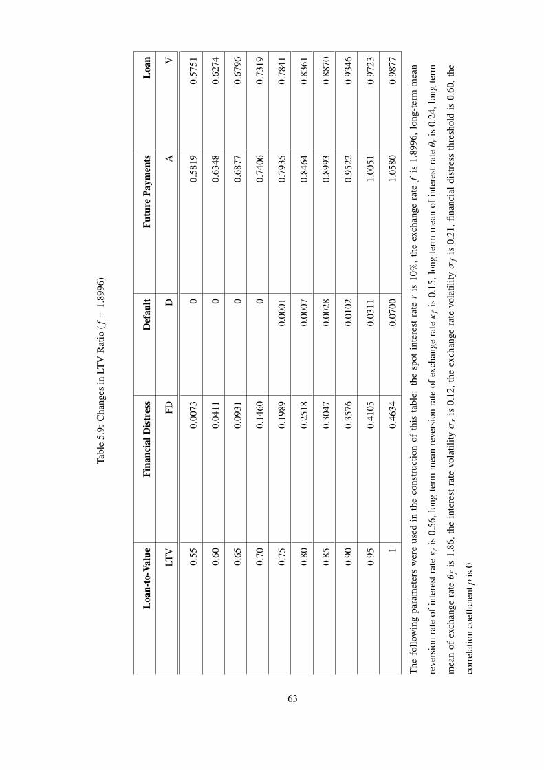
Tabl
e5.
9:C
hang
esin
LTV
Rat
io(f
=1.
8996
)
Loa
n-to
-Val
ueFi
nanc
ialD
istr
ess
Def
ault
Futu
rePa
ymen
tsL
oan
LTV
FDD
AV
0.55
0.00
730
0.58
190.
5751
0.60
0.04
110
0.63
480.
6274
0.65
0.09
310
0.68
770.
6796
0.70
0.14
600
0.74
060.
7319
0.75
0.19
890.
0001
0.79
350.
7841
0.80
0.25
180.
0007
0.84
640.
8361
0.85
0.30
470.
0028
0.89
930.
8870
0.90
0.35
760.
0102
0.95
220.
9346
0.95
0.41
050.
0311
1.00
510.
9723
10.
4634
0.07
001.
0580
0.98
77
The
follo
win
gpa
ram
eter
sw
ere
used
inth
eco
nstr
uctio
nof
this
tabl
e:th
esp
otin
tere
stra
ter
is10
%,
the
exch
ange
rate
fis
1.89
96,
long
-ter
mm
ean
reve
rsio
nra
teof
inte
rest
rateκ r
is0.
56,l
ong-
term
mea
nre
vers
ion
rate
ofex
chan
gera
teκ
fis
0.15
,lon
gte
rmm
ean
ofin
tere
stra
teθ r
is0.
24,l
ong
term
mea
nof
exch
ange
rateθ
fis
1.86
,the
inte
rest
rate
vola
tility
σr
is0.
12,t
heex
chan
gera
tevo
latil
ityσ
fis
0.21
,fina
ncia
ldis
tres
sth
resh
old
is0.
60,t
he
corr
elat
ion
coeffi
cien
tρis
0
63

Tabl
e5.
10:C
hang
esin
LTV
Rat
io(f
=2.
2388
)
Loa
n-to
-Val
ueFi
nanc
ialD
istr
ess
Def
ault
Futu
rePa
ymen
tsL
oan
LTV
FDD
AV
0.55
0.06
640
0.66
080.
652
0.60
0.12
620
0.72
090.
7112
0.65
0.18
630.
0001
0.78
090.
7705
0.70
0.24
640.
0005
0.84
100.
8295
0.75
0.30
640.
0025
0.90
110.
8876
0.80
0.36
650.
0112
0.96
110.
9412
0.85
0.42
660.
0395
1.02
120.
9805
0.90
0.48
670.
0917
1.08
130.
9894
0.95
0.54
670.
1505
1.14
140.
9909
10.
6068
0.21
041.
2014
0.99
10
The
follo
win
gpa
ram
eter
sw
ere
used
inth
eco
nstr
uctio
nof
this
tabl
e:th
esp
otin
tere
stra
ter
is10
%,
the
exch
ange
rate
fis
2.23
88,
long
-ter
mm
ean
reve
rsio
nra
teof
inte
rest
rateκ r
is0.
56,l
ong-
term
mea
nre
vers
ion
rate
ofex
chan
gera
teκ
fis
0.15
,lon
gte
rmm
ean
ofin
tere
stra
teθ r
is0.
24,l
ong
term
mea
nof
exch
ange
rateθ
fis
1.86
,the
inte
rest
rate
vola
tility
σr
is0.
12,t
heex
chan
gera
tevo
latil
ityσ
fis
0.21
,fina
ncia
ldis
tres
sth
resh
old
is0.
60,t
he
corr
elat
ion
coeffi
cien
tρis
0
64
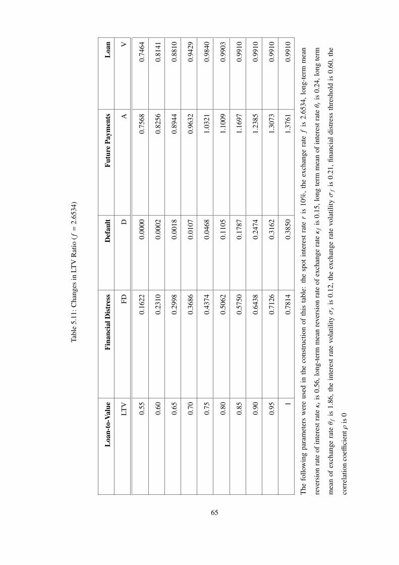
Tabl
e5.
11:C
hang
esin
LTV
Rat
io(f
=2.
6534
)
Loa
n-to
-Val
ueFi
nanc
ialD
istr
ess
Def
ault
Futu
rePa
ymen
tsL
oan
LTV
FDD
AV
0.55
0.16
220.
0000
0.75
680.
7464
0.60
0.23
100.
0002
0.82
560.
8141
0.65
0.29
980.
0018
0.89
440.
8810
0.70
0.36
860.
0107
0.96
320.
9429
0.75
0.43
740.
0468
1.03
210.
9840
0.80
0.50
620.
1105
1.10
090.
9903
0.85
0.57
500.
1787
1.16
970.
9910
0.90
0.64
380.
2474
1.23
850.
9910
0.95
0.71
260.
3162
1.30
730.
9910
10.
7814
0.38
501.
3761
0.99
10
The
follo
win
gpa
ram
eter
sw
ere
used
inth
eco
nstr
uctio
nof
this
tabl
e:th
esp
otin
tere
stra
ter
is10
%,
the
exch
ange
rate
fis
2.65
34,
long
-ter
mm
ean
reve
rsio
nra
teof
inte
rest
rateκ r
is0.
56,l
ong-
term
mea
nre
vers
ion
rate
ofex
chan
gera
teκ
fis
0.15
,lon
gte
rmm
ean
ofin
tere
stra
teθ r
is0.
24,l
ong
term
mea
nof
exch
ange
rateθ
fis
1.86
,the
inte
rest
rate
vola
tility
σr
is0.
12,t
heex
chan
gera
tevo
latil
ityσ
fis
0.21
,fina
ncia
ldis
tres
sth
resh
old
is0.
60,t
he
corr
elat
ion
coeffi
cien
tρis
0
65
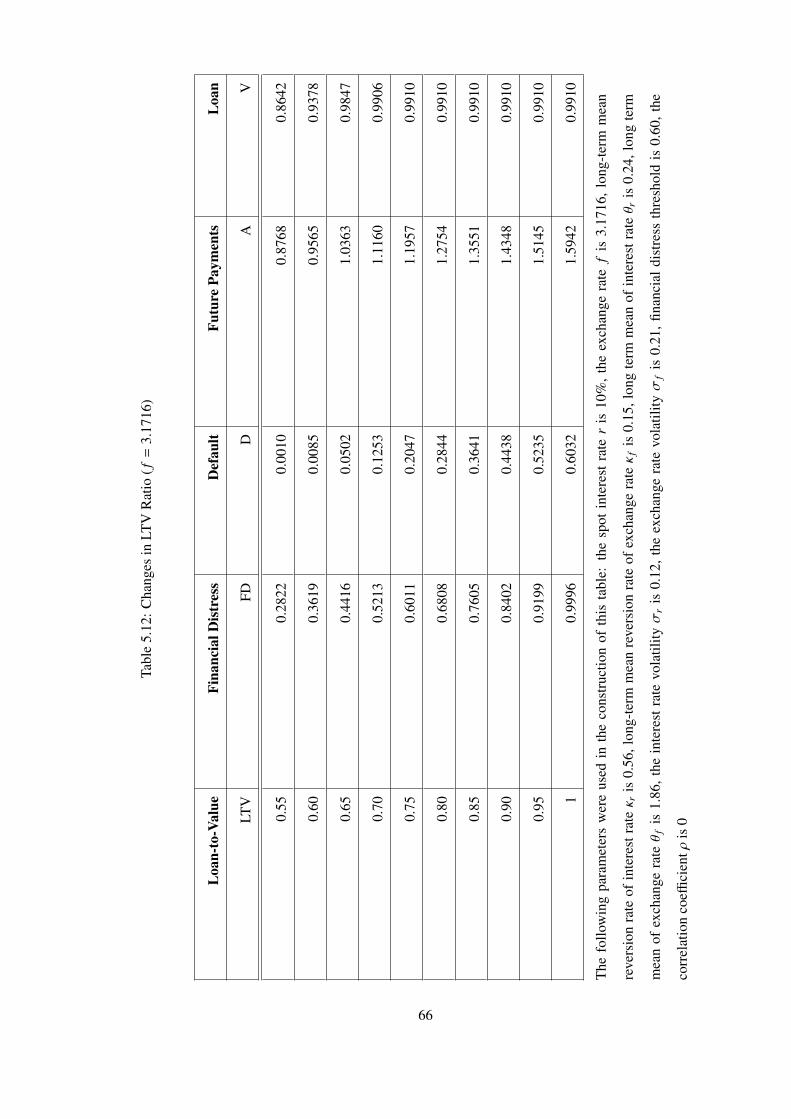
Tabl
e5.
12:C
hang
esin
LTV
Rat
io(f
=3.
1716
)
Loa
n-to
-Val
ueFi
nanc
ialD
istr
ess
Def
ault
Futu
rePa
ymen
tsL
oan
LTV
FDD
AV
0.55
0.28
220.
0010
0.87
680.
8642
0.60
0.36
190.
0085
0.95
650.
9378
0.65
0.44
160.
0502
1.03
630.
9847
0.70
0.52
130.
1253
1.11
600.
9906
0.75
0.60
110.
2047
1.19
570.
9910
0.80
0.68
080.
2844
1.27
540.
9910
0.85
0.76
050.
3641
1.35
510.
9910
0.90
0.84
020.
4438
1.43
480.
9910
0.95
0.91
990.
5235
1.51
450.
9910
10.
9996
0.60
321.
5942
0.99
10
The
follo
win
gpa
ram
eter
sw
ere
used
inth
eco
nstr
uctio
nof
this
tabl
e:th
esp
otin
tere
stra
ter
is10
%,
the
exch
ange
rate
fis
3.17
16,
long
-ter
mm
ean
reve
rsio
nra
teof
inte
rest
rateκ r
is0.
56,l
ong-
term
mea
nre
vers
ion
rate
ofex
chan
gera
teκ
fis
0.15
,lon
gte
rmm
ean
ofin
tere
stra
teθ r
is0.
24,l
ong
term
mea
nof
exch
ange
rateθ
fis
1.86
,the
inte
rest
rate
vola
tility
σr
is0.
12,t
heex
chan
gera
tevo
latil
ityσ
fis
0.21
,fina
ncia
ldis
tres
sth
resh
old
is0.
60,t
he
corr
elat
ion
coeffi
cien
tρis
0
66

Tabl
e5.
13:C
hang
esin
Fina
ncia
lDis
tres
sB
arri
er(f
=2.
2388
)
Dis
tres
sBar
rier
Fina
ncia
lDis
tres
sD
efau
ltFu
ture
Paym
ents
Loa
n
Th
FDD
AV
0.50
0.46
560.
0112
0.96
110.
9412
0.55
0.41
610.
0112
0.96
110.
9412
0.60
0.36
650.
0112
0.96
110.
9412
0.65
0.31
700.
0112
0.96
110.
9412
0.70
0.26
740.
0112
0.96
110.
9412
0.75
0.21
790.
0112
0.96
110.
9412
0.80
0.16
830.
0112
0.96
110.
9412
The
follo
win
gpa
ram
eter
sw
ere
used
inth
eco
nstr
uctio
nof
this
tabl
e:th
esp
otin
tere
stra
ter
is10
%,
the
exch
ange
rate
fis
2.23
88,
long
-ter
mm
ean
reve
rsio
nra
teof
inte
rest
rateκ r
is0.
56,l
ong-
term
mea
nre
vers
ion
rate
ofex
chan
gera
teκ
fis
0.15
,lon
gte
rmm
ean
ofin
tere
stra
teθ r
is0.
24,l
ong
term
mea
nof
exch
ange
rateθ
fis
1.86
,the
inte
rest
rate
vola
tility
σr
is0.
12,t
heex
chan
gera
tevo
latil
ityσ
fis
0.21
,LT
Vra
tiois
0.80
,the
corr
elat
ion
coeffi
cien
t
ρis
0
67

Tabl
e5.
14:C
ombi
ned
Eff
ects
ofT
han
dLT
Vra
tioon
Fina
ncia
lDis
tres
s(f
=2.
2388
)
Valu
eof
Fina
ncia
lDis
tres
s
Dis
tres
sBar
rier
LTV
Rat
ios
Th
0.60
0.65
0.70
0.75
0.80
0.85
0.90
0.95
0.50
0.22
530.
2854
0.34
550.
4055
0.46
560.
5257
0.58
580.
6458
0.55
0.17
580.
2359
0.29
590.
356
0.41
610.
4761
0.53
620.
5963
0.60
0.12
620.
1863
0.24
640.
3064
0.36
650.
4266
0.48
670.
5467
0.65
0.07
690.
1368
0.19
680.
2569
0.31
700.
377
0.43
710.
4972
0.70
0.03
050.
0874
0.14
730.
2073
0.26
740.
3275
0.38
760.
4476
0.75
0.00
690.
0404
0.09
781
0.15
780.
2179
0.27
790.
338
0.39
81
0.80
0.00
160.
0106
0.05
0.10
840.
1683
0.22
840.
2884
0.34
85
The
follo
win
gpa
ram
eter
sw
ere
used
inth
eco
nstr
uctio
nof
this
tabl
e:th
esp
otin
tere
stra
ter
is10
%,
the
exch
ange
rate
fis
2.23
88,
long
-ter
mm
ean
reve
rsio
nra
teof
inte
rest
rateκ r
is0.
56,l
ong-
term
mea
nre
vers
ion
rate
ofex
chan
gera
teκ
fis
0.15
,lon
gte
rmm
ean
ofin
tere
stra
teθ r
is0.
24,l
ong
term
mea
nof
exch
ange
rateθ
fis
1.86
,the
inte
rest
rate
vola
tility
σr
is0.
12,t
heex
chan
gera
tevo
latil
ityσ
fis
0.21
,the
corr
elat
ion
coeffi
cien
tρis
0
68

CHAPTER 6
CONCLUSION
6.1 Summary
This thesis establishes and solves a structural model for the valuation of fixed rate foreign
currency denominated corporate loans, whose conditions are identified based on non-financial
corporations’ foreign borrowing information in Turkey. Possible financial distress and default
events caused by foreign currency denominated loan issuance at the corporate level are also
priced.
First, we give an overview of the study. Foreign currency denominated corporate loan con-
tract related concepts and market information as well as the credit pricing methodologies are
introduced. Credit market in Turkey is discussed focusing on FX-loan market at the corpo-
rate level. Growing foreign currency loan shares in total corporate loans and market trends
of the specifications of the contracts are discussed. Studies on foreign exchange rate bor-
rowing and risky debt valuation techniques are reviewed. Literature on foreign borrowing
by non-financial firms mostly focuses on the financing choices of the non-financial firms and
motivations of issuing foreign currency denominated loan. In this study, possible risk factors
are mentioned and some techniques to price credit risk in literature are summarized.
The literature review guided us in the decision of employing a contingent claims framework.
We analyzed default option and financial distress in foreign currency denominated corporate
loans. We develop and evaluate a model to price the FX-loan and its related assets, which are
future payments, financial distress and default, in a framework based on the Cox, Ingersoll
and Ross [28] equilibrium model. The main risk factors are identified as the interest rate
69

and the exchange rate. Two-factor formulation is employed following this assumption where
state variables are the main risk factors. The corresponding valuation function is a partial
differential equation for which there is no closed form solution. Consequently, we employ
a numerical solution technique. Valuation functions for monthly payments, borrower’s debt,
remaining payments, default and financial distress are developed according to their payment
behaviors. Since the value of the different assets is known at termination of the contract, once
the boundary conditions are identified, the model is closed and can be solved recursively using
backward solution techniques.
The explicit finite difference method is used to solve the problem. The necessary steps to find a
numerical solution such as transforming the original PDE and mapping its original bi-infinite
domain into a unit square are also explained. The stability of the model is maintained by use
of an ”upwind differencing” scheme and difference equations are generated. Considering the
original PDE the common boundary conditions are formulated. All the required conditions
for the solution of the problem are obtained. Lastly, MATLAB code is developed to find a
numerical solution.
This thesis provides a valuable study in order to evaluate foreign currency risk and interest
rate risk with the corresponding financial distress and default risks of foreign currency de-
nominated loans under volatile economic conditions. Numerical results were evaluated for
different contract specifications and for different economic environments. Results for the val-
ues of foreign currency denominated corporate loan related assets are interpreted in terms of
mathematical and financial perspectives. Values of default and financial distress are calcu-
lated according to the capital structure of a non-financial firm. The results are consistent with
the economic knowledge and suggest that increase in exchange rate and decrease in interest
rate (discount rate) cause financial distress and triggers the event of default for corporations.
The findings reveal that the effect of an increment in exchange rate is sharper than the effect
of a decrement in interest rate on financial distress and default values. Recently, Turkish lira
has rapidly devaluated against dollar, euro and pound. Under these conditions, both finan-
cial distress and default risks for sectors that are heavily financed by FX-loans increase. Our
results indicate that interest rate volatility is reasonably more effective on financial distress
and default risk in comparison to exchange rate volatility. Another important result is that
non-financial firms having high ratio of foreign currency loan to total assets are exposed to
default risk and financial distress. Furthermore, high values of exchange rate and low values
70
of spot interest rate trigger the events of default and financial distress to occur with values that
cannot be neglected. However, even when there is an economical crisis, such default event
hasn’t been observed in Turkey, which can be attributable to the firms’ effective management
of foreign exchange risk.
After 2001 financial crisis, Turkey has experienced higher interest rates and lower exchange
rates compared to the pre-2001 period. Higher interest rates can be defined as the higher op-
portunity cost of capital from the financial perspective. As the cost of borrowing in domestic
currency increases, our results suggest that we would expect to see lower financial distress for
corporations that are heavily financed by FX-loans. Firms used that opportunity by financing
their operations heavily by FX-loans and in most of the sectors, especially in utilities sector,
the share of FX-loans in total borrowing of the non-financial firms increased significantly.
Since 2008 CBRT has decreased borrowing rates and very recently, Turkish lira has rapidly
devaluated against dollar and euro. Our results show that if volatility in exchange rates leads
to higher exchange rates, then the financial distress and default values for the sectors that are
heavily financed by FX-loans increase in an economic environment where volatility of inter-
est rate is also high. The values obtained for financial distress and default are also interpreted
as the amounts of hedged positions, that firms should have in their capital structure to avoid
financial distress and default, in terms of total assets value of the firms.
6.2 Contributions of the Research and Further Study
To the best of our knowledge, this thesis contributes to the extant literature by providing the
first study that develops a structural model to evaluate foreign currency denominated corporate
loans in option pricing framework. Details of the pricing model also yield some contributions.
Methodological contributions can be summarized as follows. Our model assumes that the
value of firm’s assets is constant and uses two state variables; namely, the interest rate and
exchange rate, both of which follow CIR process. In addition, the main partial differential
equation used in the study differs according to the choice of stochastic processes for the state
variables compared to its counterparts.
In the existing literature, pricing default risk and financial distress in FX-loans at corporate
level has not been studied. This study contributes to the literature on contingent claims pricing
71

framework for the valuation of foreign currency denominated corporate debt by measuring
the corresponding default risk and financial distress values for non-financial firms. Recent
global trends show that non-financial firms, especially firms in utilities sector, are heavily
financed by FX-loans. Turkish firms in utilities sector also follow the global trend in using
FX-loans widely. We observe that under the volatile economic environment in Turkey, these
companies can still survive. This thesis demonstrates that although companies experience
financial distress, especially with high LTV FX-loans where FX-rates are high they can still
continue their operations. We conclude that firms may go into bankruptcy (or default) if they
borrow 95% to 100% LTV loans with considerably high FX-rates ( f = 2.2388, 2.6534 ),
especially when interest rates considerably volatile.
The present study models exchange rate variable as a CIR process. Therefore, big discon-
tinuities in exchange rate movements in the real world are neglected. In order to integrate
such discontinuities of the exchange rate movements into the FX-loan pricing model, a jump
process can be used to model the exchange rate in a further study. This study also assumes
that the value of firm’s assets is constant during the life of the loan. The effect of the asset
value of the firm on foreign currency denominated loan can further be studied and evaluated
by developing a three factor model. Finally, a finite volume model can be developed to find a
corresponding numerical solution of a three factor model.
72

REFERENCES
[1] Goswami, G., Shrikhande, M., M., Economic exposure and debt financing choice, Jour-nal of Multinational Financial Management, 2001.
[2] Kedia, S., Mozumdar, A., Foreign currency denominated debt: an empirical examina-tion, The Journal of Business, 2003.
[3] Global Development Finance 2009, The World Bank, www.worldbank.org/gdf2009,2009.
[4] Financial Stability Report, Central Bank of the Republic of Turkey, 2010.
[5] Kiymaz, H., Estimation of foreign exchange exposure: an emerging market application,Journal of Multinational Financial Management, 2003.
[6] Kwon, H., T., Bae, C., S., Asymmetric Foreign Exchange Exposure and Foreign Cur-rency Denominated Debt: International Evidence, 2010.
[7] Allayannis, G., Brown, W., G., Klapper, F., L., Capital Structure and Financial Risk:Evidence From Foreign Debt Use in East Asia
[8] Keloharju, M., Niskanen, M., Why Do Firms Raise Foreign Currency DenominatedDebt? Evidence from Finland, European Financial Management, 2001.
[9] Aliber, Z., R., The Debt Denomination Decision, The Handbook of International Finan-cial Management, 1989.
[10] Bradley, K., Moles, P., Managing strategic exchange rate exposures: evidence from UKfirms, Managerial Finance, 2002.
[11] Bradley, K., Moles, P., The effects of exchange rate movements on non-financial UKfirms, International Business Review, 2001.
[12] Aabo, T., The Importance of Corporate Foreign Debt in Managing Exchange Rate Ex-posures in Non-Financial Companies, European Financial Management, 2006.
[13] Geczy, C., Minton, A.,B., Schrand, C., Why Firms Use Currency Derivatives, The Jour-nal of Finance, 1997.
[14] Graham, R., J., Harvey, R., C., The theory and practice of corporate finance: Evidencefrom the field, The Theory and Practice of Corporate Finance, 2001.
[15] Black, F., Scholes, M., The pricing of Options and Coporate Liabilities, Journal of Po-litical Economy, 1973.
[16] Merton, R., C., On the Pricing of Corporate Debt: The Risk Structure of Interest Rates,The Journal of Finance,1974.
73

[17] Jarrow, R., A., Turnbull, M.,S., Pricing derivatives on Financial Securities Subject toCredit Risk, The Journal of Finance, 1995.
[18] Black, F., Cox, C., J., Valuing Corporate Securities: Some Effects of Bond IndentureProvisions, The Journal of Finance, 1976.
[19] Shimko, D., Tejima, N., Van Deventer, D, The Pricing of Risky Debt When Interest Ratesare Stochastic, Journal of Fixed Income, 1993.
[20] Longstaff, A., F., Schwartz, S., E., A simple Approach to Valuing Risky Fixed and Float-ing Rate Debt, Journal of Finance, 1995.
[21] Kim, J., I., Ramaswamy, K., Sundersan, S., Does Default Risk in Coupons Affect theValuation of Corporate Bonds?: A Contingent Claims Model, Financial Management,1993.
[22] Ericsson, J., Reneby, J., A Framework for Valuing Corporate Securities, Working Paper,Stockholm School of Economics, 1995.
[23] Briys, E., de Varenne, F., Valuing Risky Fixed Rate Debt: An Extension, Journal ofFinancial and Quantitative Analysis, 1997.
[24] Leland, E., H., Corporate Debt Value, Bond Covenants, and Optimal Capital Structure,The Journal of Finance, 1994.
[25] Toft, B., K., Prucyk, B., Options on Leveraged Equity: Theory and Emprical Test, TheJournal of Finance, 1997.
[26] Opler, C., T., Titman, S., Financial Distress and Corporate Performance, The Journalof Finance, 1994.
[27] Hekman, C., R., A Financial Model for Foreign Exchange Exposure, Journal of Interna-tional Business Studies, 1985.
[28] Cox, J. C., Ingersoll and S. A. Ross, An Intertemporal General Equilibrium Model ofAsset Prices, Econometrica, 1985.
[29] Morton, K. W., Mayers and D. F., Numerical Solutions of Partial Differential Equations,Cambridge University Press, 1994
[30] Wilmott, P., Dewynne, J., Howison, S., Option Pricing: Mathematical Models and Com-putation, Oxford Financial Press, 1993
[31] Trigeorgis, L., Real Options: Managerial Flexibility and Strategy in Resource Alloca-tion, MIT Press, 1996
[32] Azevedo-Pereira, J. A., Fixed Rate Mortgage Valuation Using A Contingent Claims Ap-proach, Ph.D. Thesis submitted to the University of Manchester, 1997
[33] Schmid, B., Credit Risk Pricing Models: Theory and Practice , Springer, 2004
[34] The Relationship Between Default Risk and Interest Rates: An Emprical Study, Moody’sAnalytics, 2009
[35] Adler, M., Dumas, B.,Exposure to currency risk: definition and measurement, FinancialManagemet, 1984
74

[36] Dumas, B., The theory of the trading firm revisited, Journal of Finance, 1978
[37] Solakoglu, M., N., Exchange Rate Exposure and Firm - Specific Factors: Evidence fromTurkey, Journal of Economic and Social Research, 2005
[38] Vasicek, O., A., An Equilibrium Characterization of the Term Structure, Journal of Fi-nance, 1977
[39] Stanton, R., Rational Prepayment and the Valuation of Mortgage-Backed Securities, Thereview of Financial Studies, 1995
[40] Epperson, J.F., Kau, J.B., Keenan, D.C., Muller III., W.J. Pricing Default Risk in Mort-gages,AREUEA Journal, 1985
[41] Goldstein, M., Turner, P., Controlling currency mismatches in emerging markets , Peter-son Institute, 2004
[42] Financial Stability Review, European Central Bank,http://www.ecb.int/pub/fsr/html/index.en.html, June 2010.
[43] Gray, D., Malone, S., Macrofinancial Risk Analysis, Wiley, 2008
[44] Erol, I., Pricing Wage-Indexed Payment Mortgage Contract and the Default Risk in theTurkish Mortgage Market, Ph.D. Thesis, 2004
[45] Grinblatt, M., Titman, S., Financial Markets and Corporate Strategy, McGraw-Hill ,2001
75

APPENDIX A
Matlab Code for Consistency, Stability and Convergence of the
Transformed PDE
function[CO]=Consistency(InputData)
%%%%%%%%%%%%%%%%%%%%%%%%%%%%%%%%%%%%%%%%%%%%
%’InputData’ is the matrix of external parameters in the value of fix rate
%foreign currency denominated loan. The rows of the matrix are composed
%as following%
%InputData(1)=contract maturity
%InputData(2)= time step per month
%InputData(3)= long-term mean reversion rate of interest rate
%InputData(4)= long term mean of interest rate
%InputData(5)= interest rate volatility
%InputData(6)= long-term mean reversion rate of exchange rate
%InputData(7)= long term mean of exchange rate
%InputData(8)= exchange rate volatility
%InputData(9)= scale factor for interest rate transformation
%InputData(10)= scale factor for fx rate transformation
%InputData(11)= correlation coefficient
%InputData(12)= initial Loan value
%InputData(13)= coupon rate
%InputData(14)= # grid points in x direction
%InputData(15)= # grid points in y direction
%InputData(16)=Threshold
76

%InputData(17)=VA
%InputData(18)=initial fx rate
%%%%%%%%%%%%%%%%%%%%%%%%%%%%%%%%%%%%%%%%%%%
InputData=[ 60.0000,66.0000,0.5600,0.2400,0.1200,0.1500,1.8600,0.2100,...
10.0000,0.67, 0,0.9500,0.1000,50.0000,50.0000,0.6000,1.0000,1.5230];
%%%%%%%%%%%%%%%%%%%%%%
%Internal Parameters
%%%%%%%%%%%%%%%%%%%%%
%cn is the counter for months, cs is the counter for time steps, cx is the
%counter for fx-rate dimension, cy is the counter
%for interest rate dimension. ”.....inc” represents the increment for the
%variable ”.....”
cnmin=1;
cnmax=InputData(1);
cninc=1;
s=1/(12*InputData(2));
csmin=1;
csmax=csmin+InputData(2);
csinc=1;
cxmin=1;
cxmax=cxmin+InputData(14);
cxinc=1;
cymin=1;
cymax=cymin+InputData(15);
cyinc=1;
77

% ”x” is the transformed varible in the fx-rate dimension. So the grid
% will be linear in x but not in F (fx-rate)
xmin=0;
xmax=1;
xinc=1/InputData(14);
x=xmin:xinc:xmax;
% y is the transformed varible in the interest rate dimension. So the grid
% will be linear in y but not in R (interest rate)
ymin=0;
ymax=1;
yinc=1/InputData(15);
y=ymin:yinc:ymax;
cxhalf=cxmin+round(InputData(14)/2);
cyhalf=cymin+round(InputData(15)/2);
%%%%%%%%%%%%%%%%%%%%%%%%%%%%%%
%Preliminary Calculations
%%%%%%%%%%%%%%%%%%%%%%%%%%%%%%
%The Value of fx-rate
F(cxmax)=0;
F(cxmin)=inf;
for cx=cxmin+1:cxmax-1
F(cx)=(1-x(cx))/(InputData(10)*x(cx));
end
%The Value of Interest Rate
R(cymax)=0;
78

R(cymin)=inf;
for cy=cymin+1:cymax-1
R(cy)=(1-y(cy))/(InputData(9)*y(cy));
end
for cy=cymin+1:cymax
for cx=cxmin+1:cxmax
Term2=0.5*R(cy)*(InputData(5)ˆ2)*(InputData(9)ˆ2*...
(y(cy)ˆ4));
Term3=0.5*F(cx)*(InputData(8)ˆ2)*(InputData(10)ˆ2*...
(x(cx)ˆ4));
C(cy,cx)= Term2*(s/(xincˆ2))+ Term3*(s/(yincˆ2));
end
end
%For matrices, MAX(X) is a row vector containing
%the maximum element from each column.
MaxC=max(max(C))
[CO]=[C];
end
79

APPENDIX B
Matlab Code for Loan Valuation
function[FR]=LoanValuation(InputData)
%%%%%%%%%%%%%%%%%%%%%%%%%%%%%%%%%%%%%%%%%%%
%’InputData’ is the matrix of external parameters in the value of fix rate
%foreign currency denominated loan.
%The rows of the matrix are composed as following%
%InputData(1)=contract maturity
%InputData(2)= time step per month
%InputData(3)= long-term mean reversion rate of interest rate
%InputData(4)= long term mean of interest rate
%InputData(5)= interest rate volatility
%InputData(6)= long-term mean reversion rate of exchange rate
%InputData(7)= long term mean of exchange rate
%InputData(8)= exchange rate volatility
%InputData(9)= scale factor for interest rate transformation
%InputData(10)= scale factor for fx rate transformation
%InputData(11)= correlation coefficient
%InputData(12)= initial Loan Value
%InputData(13)= coupon rate
%InputData(14)= # grid points in x direction
%InputData(15)= # grid points in y direction
%InputData(16)=Threshold
%InputData(17)=VA
%InputData(18)=initial fx rate
80
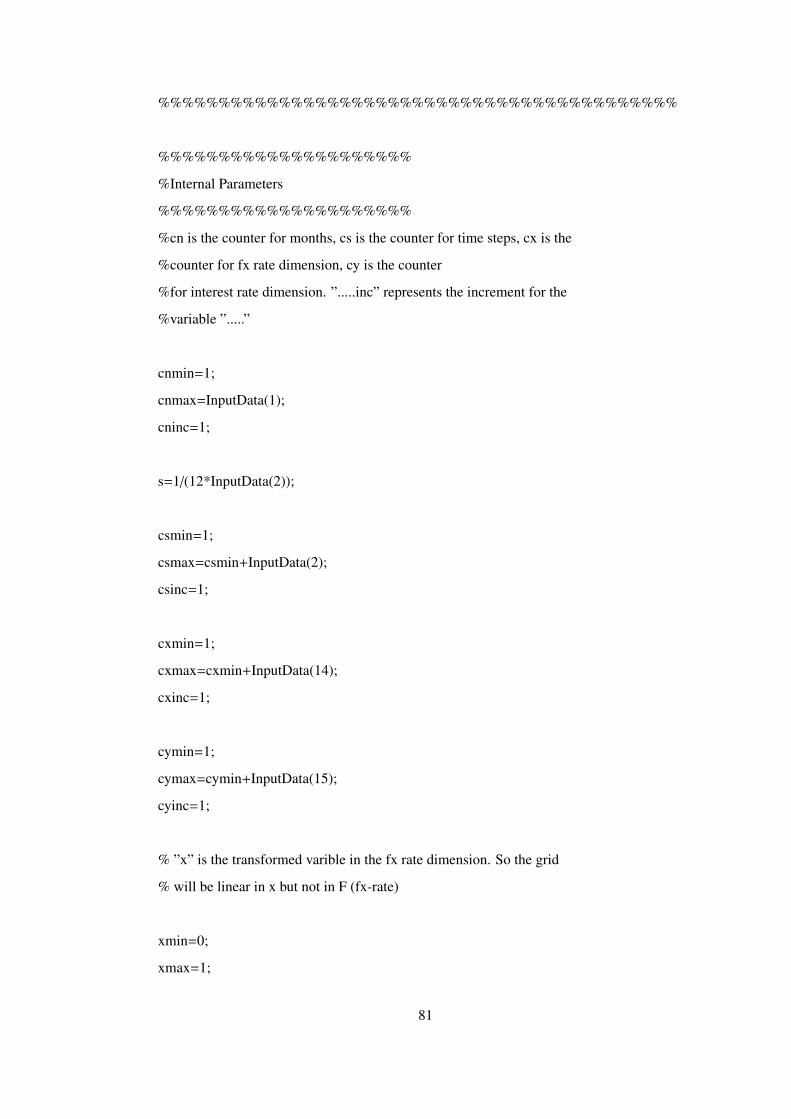
%%%%%%%%%%%%%%%%%%%%%%%%%%%%%%%%%%%%%%%%%%%
%%%%%%%%%%%%%%%%%%%%%
%Internal Parameters
%%%%%%%%%%%%%%%%%%%%%
%cn is the counter for months, cs is the counter for time steps, cx is the
%counter for fx rate dimension, cy is the counter
%for interest rate dimension. ”.....inc” represents the increment for the
%variable ”.....”
cnmin=1;
cnmax=InputData(1);
cninc=1;
s=1/(12*InputData(2));
csmin=1;
csmax=csmin+InputData(2);
csinc=1;
cxmin=1;
cxmax=cxmin+InputData(14);
cxinc=1;
cymin=1;
cymax=cymin+InputData(15);
cyinc=1;
% ”x” is the transformed varible in the fx rate dimension. So the grid
% will be linear in x but not in F (fx-rate)
xmin=0;
xmax=1;
81

xinc=1/InputData(14);
x=xmin:xinc:xmax;
% y is the transformed varible in the interest rate dimension. So the grid
% will be linear in y but not in R (interest rate)
ymin=0;
ymax=1;
yinc=1/InputData(15);
y=ymin:yinc:ymax;
cxhalf=cxmin+round(InputData(14)/2);
cyhalf=cymin+round(InputData(15)/2);
%%%%%%%%%%%%%%%
%Preliminary Calculations
%%%%%%%%%%%%%%%
%The value of fx-rate
F(cxmax)=0;
F(cxmin)=inf;
for cx=cxmin+1:cxmax-1
F(cx)=(1-x(cx))/(InputData(10)*x(cx));
end
%the value of interest rate
R(cymax)=0;
R(cymin)=inf;
for cy=cymin+1:cymax-1
R(cy)=(1-y(cy))/(InputData(9)*y(cy));
end
82

%%%%%%%%%%%%%%%%%%%%%%%%%%%%%%
%FINAL TERMINATION CONDITIONS
%%%%%%%%%%%%%%%%%%%%%%%%%%%%%%
%Valuation of monthly payment
M=(((InputData(13)/12)*(1+(InputData(13)/12))ˆcnmax)/...
((1+(InputData(13)/12))ˆcnmax-1))*InputData(12)/InputData(18);
for cy=cymin:cymax
for cx=cxmin+1:cxmax-1
NewA(cy,cx)=M*F(cx);
OldA(cy,cx)=NewA(cy,cx);
end
% F is infinite (cx=cxmin)
NewA(cy,cxmin)=InputData(17);
OldA(cy,cxmin)=NewA(cy,cxmin);
% F is zero (cx=cxmax)
NewA(cy,cxmax)=0;
OldA(cy,cxmax)=NewA(cy,cxmax);
end
for cy=cymin:cymax
for cx=cxmin+1:cxmax
OldFD(cy,cx)=max(0,M*F(cx)-InputData(16));
OldD(cy,cx)=max(0,M*F(cx)-InputData(17));
OldV(cy,cx)=min(M*F(cx),InputData(17));
end
83
%F is infinite(cx=cxmin)
OldFD(cy,cxmin)=InputData(17);
OldV(cy,cxmin)=InputData(17);
OldD(cy,cxmin)=InputData(17);
end
%%%%%%%%%%%%%%%%%%%%%%%%
%The Beginning of the Last Month
%%%%%%%%%%%%%%%%%%%%%%%
cn=cnmin;
for cs=csmin:csmax
%%%BOUNDARY CONDITIONS%%%%
%The Value of A(R,F) at the Corners
NewA(cymax,cxmin)=OldA(cymax-1,cxmin);
OldA(cymax,cxmin)=NewA(cymax,cxmin);
NewA(cymax,cxmax)=OldA(cymax-1,cxmax);
OldA(cymax,cxmax)=NewA(cymax,cxmax);
NewA(cymin,cxmin)=0;
OldA(cymin,cxmin)=NewA(cymin,cxmin);
NewA(cymin,cxmax)=0;
OldA(cymin,cxmax)=NewA(cymin,cxmax);
%The value of A(R,F) at the Edges
%F=0 R varies%
for cy=cymin+1:cymax-1
84

NewA(cy,cxmax)=0;
OldA(cy,cxmax)=NewA(cy,cxmax);
end
%R=0, F varies%
for cx=cxmin+1:cxmax-1
Term7=1-F(cx)*(InputData(8)ˆ2)*(InputData(10)ˆ2*...
(x(cx)ˆ4)*(s/xincˆ2));
Term8=0.5*F(cx)*(InputData(8)ˆ2)*(InputData(10)ˆ2*...
(x(cx)ˆ4)*(s/xincˆ2));
Term9=(F(cx)*(InputData(8)ˆ2)*(InputData(10)ˆ2)*...
(x(cx)ˆ3)-(InputData(6)*(InputData(7)-F(cx))*...
InputData(10)*(x(cx)ˆ2)))*(s/xinc);
Term10=-InputData(3)*InputData(4)*InputData(9)*(y(cy)ˆ2)*(s/yinc);
EQ3=(F(cx)*(InputData(8)ˆ2)*(InputData(10)ˆ2)*...
(x(cx)ˆ3)-(InputData(6)*(InputData(7)-F(cx))*...
InputData(10)*(x(cx)ˆ2)));
if EQ3<0
NewA(cymax,cx)=Term7*OldA(cymax,cx)+...
Term8*(OldA(cymax,cx+1)-OldA(cymax,cx-1))+...
Term10*(OldA(cymax,cx)-OldA(cymax-1,cx))+...
Term9*(OldA(cymax,cx)- OldA(cymax,cx-1));
else
NewA(cymax,cx)=Term7*OldA(cymax,cx)+...
Term8*(OldA(cymax,cx+1)-OldA(cymax,cx-1))+...
Term10*(OldA(cymax,cx)-OldA(cymax-1,cx))+...
Term9*(OldA(cymax,cx+1)- OldA(cymax,cx));
end
OldA(cymax,cx)=NewA(cymax,cx);
85

end
%F=inf, R varies%
for cy=cymin+1:cymax-1
Term11=1-R(cy)*(InputData(5)ˆ2)*(InputData(9)ˆ2*...
(y(cy)ˆ4)*(s/yincˆ2))-R(cy)*s;
Term12=0.5*R(cy)*(InputData(5)ˆ2)*(InputData(9)ˆ2*...
(y(cy)ˆ4)*(s/yincˆ2));
Term13=(R(cy)*(InputData(5)ˆ2)*(InputData(9)ˆ2)*...
(y(cy)ˆ3)-(InputData(3)*(InputData(4)-R(cy))*...
InputData(9)*(y(cy)ˆ2)))*(s/yinc);
Term14=-(InputData(6)*InputData(7)*InputData(10)*(x(cx)ˆ2))*(s/xinc);
EQ4=(R(cy)*(InputData(5)ˆ2)*(InputData(9)ˆ2)*...
(y(cy)ˆ3)-(InputData(3)*(InputData(4)-R(cy))*...
InputData(9)*(y(cy)ˆ2)));
if EQ4<0
NewA(cy,cxmin)=Term11*OldA(cy,cxmin)+...
Term12*(OldA(cy+1,cxmin)+OldA(cy-1,cxmin))+...
Term13*(OldA(cy,cxmin)-OldA(cy-1,cxmin))+...
Term14*(OldA(cy,cxmin)- OldA(cy,cxmin+1));
else
NewA(cy,cxmin)=Term11*OldA(cy,cxmin)+...
Term12*(OldA(cy+1,cxmin)+OldA(cy-1,cxmin))+...
Term13*(OldA(cy+1,cxmin)-OldA(cy,cxmin))+...
Term14*(OldA(cy,cxmin)- OldA(cy,cxmin+1));
end
OldA(cy,cxmin)=NewA(cy,cxmin);
end
86
%R=inf, F varies%
for cx=cxmin+1:cxmax-1
NewA(cymin,cx)=0;
OldA(cymin,cx)=NewA(cymin,cx);
end
%PDE solution for A(R,F)%
for cy=cymin+1:cymax-1
for cx=cxmin+1:cxmax-1
Term1=1-R(cy)*(InputData(5)ˆ2)*(InputData(9)ˆ2*...
(y(cy)ˆ4)*(s/yincˆ2))-F(cx)*(InputData(8)ˆ2)*...
(InputData(10)ˆ2*(x(cx)ˆ4)*(s/xincˆ2))-R(cy)*s;
Term2=0.5*R(cy)*(InputData(5)ˆ2)*(InputData(9)ˆ2*...
(y(cy)ˆ4)*(s/(yincˆ2)));
Term3=0.5*F(cx)*(InputData(8)ˆ2)*(InputData(10)ˆ2*...
(x(cx)ˆ4)*(s/(xincˆ2)));
Term4=(R(cy)*(InputData(5)ˆ2)*(InputData(9)ˆ2)*...
(y(cy)ˆ3)-(InputData(3)*(InputData(4)-R(cy))*...
InputData(9)*(y(cy)ˆ2)))*(s/yinc);
Term5=(F(cx)*(InputData(8)ˆ2)*(InputData(10)ˆ2)*...
(x(cx)ˆ3)-(InputData(6)*(InputData(7)-F(cx))*...
InputData(10)*(x(cx)ˆ2)))*(s/xinc);
Term6=InputData(11)*InputData(5)*InputData(8)*...
(R(cy)ˆ0.5)*(F(cx)ˆ0.5)*InputData(9)*InputData(10)*...
y(cy)ˆ2*x(cx)ˆ2*(s/(4*xinc*yinc));
EQ1=(F(cx)*(InputData(8)ˆ2)*(InputData(10)ˆ2)*...
(x(cx)ˆ3)-(InputData(6)*(InputData(7)-F(cx))*...
InputData(10)*(x(cx)ˆ2)));
EQ2=(R(cy)*(InputData(5)ˆ2)*(InputData(9)ˆ2)*...
87

(y(cy)ˆ3)-(InputData(3)*(InputData(4)-R(cy))*...
InputData(9)*(y(cy)ˆ2)));
if EQ1>=0 && EQ2>=0
NewA(cy,cx)=Term1*OldA(cy,cx)+...
Term2*(OldA(cy+1,cx)+OldA(cy,cx))+...
Term3*(OldA(cy,cx+1)+OldA(cy,cx-1))+...
Term4*(OldA(cy+1,cx)-OldA(cy,cx))+...
Term5*(OldA(cy,cx+1)- OldA(cy,cx))+...
Term6*(OldA(cy+1,cx+1)-OldA(cy-1,cx+1)-...
OldA(cy+1,cx-1)+OldA(cy-1,cx-1));
elseif EQ1<0 && EQ2>=0
NewA(cy,cx)=Term1*OldA(cy,cx)+...
Term2*(OldA(cy+1,cx)+OldA(cy-1,cx))+...
Term3*(OldA(cy,cx+1)+OldA(cy,cx-1))+...
Term4*(OldA(cy+1,cx)-OldA(cy,cx))+...
Term5*(OldA(cy,cx)-OldA(cy,cx-1))+...
Term6*(OldA(cy+1,cx+1)-OldA(cy-1,cx+1)-...
OldA(cy+1,cx-1)+OldA(cy-1,cx-1));
elseif EQ1>=0 && EQ2<0
NewA(cy,cx)=Term1*OldA(cy,cx)+...
Term2*(OldA(cy+1,cx)+OldA(cy-1,cx))+...
Term3*(OldA(cy,cx+1)+OldA(cy,cx-1))+...
Term4*(OldA(cy,cx)-OldA(cy-1,cx))+...
Term5*(OldA(cy,cx+1)-OldA(cy,cx))+...
Term6*(OldA(cy+1,cx+1)-OldA(cy-1,cx+1)-...
OldA(cy+1,cx-1)+OldA(cy-1,cx-1));
else
NewA(cy,cx)=Term1*OldA(cy,cx)+...
88

Term2*(OldA(cy+1,cx)+OldA(cy-1,cx))+...
Term3*(OldA(cy,cx+1)+OldA(cy,cx-1))+...
Term4*(OldA(cy,cx)-OldA(cy-1,cx))+...
Term5*(OldA(cy,cx)-OldA(cy,cx-1))+...
Term6*(OldA(cy+1,cx+1)-OldA(cy-1,cx+1)-...
OldA(cy+1,cx-1)+OldA(cy-1,cx-1));
end
OldA(cy,cx)=NewA(cy,cx);
end
end
%%%%Corners of the Grid %%%
%Corners of the grid in which F=0, R=0 %%%
NewV(cymax,cxmax)=OldV(cymax-1,cxmax);
NewD(cymax,cxmax)=OldD(cymax-1,cxmax);
NewFD(cymax,cxmax)=OldFD(cymax-1,cxmax);
OldV(cymax,cxmax)=NewV(cymax,cxmax);
OldD(cymax,cxmax)=NewD(cymax,cxmax);
OldFD(cymax,cxmax)=NewFD(cymax,cxmax);
%Corners of the grid in which F=inf, R=0 %%%
NewV(cymax,cxmin)=OldV(cymax-1,cxmin);
NewD(cymax,cxmin)=OldD(cymax-1,cxmin);
NewFD(cymax,cxmin)=OldFD(cymax-1,cxmin);
OldV(cymax,cxmin)=NewV(cymax,cxmin);
OldD(cymax,cxmin)=NewD(cymax,cxmin);
OldFD(cymax,cxmin)=NewFD(cymax,cxmin);
89

%Corners of the grid in which F=inf, R=inf %%%
NewV(cymin,cxmin)=0;
NewD(cymin,cxmin)=0;
NewFD(cymin,cxmin)=0;
OldV(cymin,cxmin)=NewV(cymin,cxmin);
OldD(cymin,cxmin)=NewD(cymin,cxmin);
OldFD(cymin,cxmin)=NewFD(cymin,cxmin);
%Corners of the grid in which F=0, R=inf %%%
NewV(cymin,cxmax)=0;
NewD(cymin,cxmax)=0;
NewFD(cymin,cxmax)=0;
OldV(cymin,cxmax)=NewV(cymin,cxmax);
OldD(cymin,cxmax)=NewD(cymin,cxmax);
OldFD(cymin,cxmax)=NewFD(cymin,cxmax);
%%%%Edges of the Grid %%%%
%F=0 R varies%
for cy=cymin+1:cymax-1
NewD(cy,cxmax)=0;
NewFD(cy,cxmax)=0;
NewV(cy,cxmax)=0;
OldD(cy,cxmax)=NewD(cy,cxmax);
OldFD(cy,cxmax)=NewFD(cy,cxmax);
OldV(cy,cxmax)=NewV(cy,cxmax);
end
%R=0, F varies%
for cx=cxmin+1:cxmax-1
Term15=1-F(cx)*(InputData(8)ˆ2)*(InputData(10)ˆ2)*...
(x(cx)ˆ4)*(s/(xincˆ2));
90

Term16=0.5*F(cx)*(InputData(8)ˆ2)*(InputData(10)ˆ2)*...
(x(cx)ˆ4)*(s/(xincˆ2));
Term17=(F(cx)*(InputData(8)ˆ2)*(InputData(10)ˆ2)*...
(x(cx)ˆ3)-(InputData(6)*(InputData(7)-F(cx))*...
InputData(10)*(x(cx)ˆ2)))*(s/xinc);
Term18=-InputData(3)*InputData(4)*InputData(9)*...
(y(cy)ˆ2)*(s/yinc);
EQ5=(F(cx)*(InputData(8)ˆ2)*(InputData(10)ˆ2)*...
(x(cx)ˆ3)-(InputData(6)*(InputData(7)-F(cx))*...
InputData(10)*(x(cx)ˆ2)));
if EQ5<0
NewV(cymax,cx)=Term15*OldV(cymax,cx)+...
Term16*(OldV(cymax,cx+1)-OldV(cymax,cx-1))+...
Term18*(OldV(cymax,cx)-OldV(cymax-1,cx))+...
Term17*(OldV(cymax,cx)- OldV(cymax,cx-1));
OldV(cymax,cx)=NewV(cymax,cx);
NewD(cymax,cx)=Term15*OldD(cymax,cx)+...
Term16*(OldD(cymax,cx+1)-OldD(cymax,cx-1))+...
Term18*(OldD(cymax,cx)-OldD(cymax-1,cx))+...
Term17*(OldD(cymax,cx)- OldD(cymax,cx-1));
OldD(cymax,cx)=NewD(cymax,cx);
NewFD(cymax,cx)=Term15*OldFD(cymax,cx)+...
Term16*(OldFD(cymax,cx+1)-OldFD(cymax,cx-1))+...
Term18*(OldFD(cymax,cx)-OldFD(cymax-1,cx))+...
Term17*(OldFD(cymax,cx)- OldFD(cymax,cx-1));
OldFD(cymax,cx)=NewFD(cymax,cx);
else
NewV(cymax,cx)=Term15*OldV(cymax,cx)+...
Term16*(OldV(cymax,cx+1)-OldV(cymax,cx-1))+...
91

Term18*(OldV(cymax,cx)-OldV(cymax-1,cx))+...
Term17*(OldV(cymax,cx+1)- OldV(cymax,cx));
OldV(cymax,cx)=NewV(cymax,cx);
NewD(cymax,cx)=Term15*OldD(cymax,cx)+...
Term16*(OldD(cymax,cx+1)-OldD(cymax,cx-1))+...
Term18*(OldD(cymax,cx)-OldD(cymax-1,cx))+...
Term17*(OldD(cymax,cx+1)- OldD(cymax,cx));
OldD(cymax,cx)=NewD(cymax,cx);
NewFD(cymax,cx)=Term15*OldFD(cymax,cx)+...
Term16*(OldFD(cymax,cx+1)-OldFD(cymax,cx-1))+...
Term18*(OldFD(cymax,cx)-OldFD(cymax-1,cx))+...
Term17*(OldFD(cymax,cx+1)- OldFD(cymax,cx));
OldFD(cymax,cx)=NewFD(cymax,cx);
end
end
%F=inf, R varies%
for cy=cymin+1:cymax-1
Term19=1-R(cy)*(InputData(5)ˆ2)*(InputData(9)ˆ2*...
(y(cy)ˆ4)*(s/yincˆ2))-R(cy)*s;
Term20=0.5*R(cy)*(InputData(5)ˆ2)*(InputData(9)ˆ2*...
(y(cy)ˆ4)*(s/yincˆ2));
Term21=(R(cy)*(InputData(5)ˆ2)*(InputData(9)ˆ2)*...
(y(cy)ˆ3)-(InputData(3)*(InputData(4)-R(cy))*...
InputData(9)*(y(cy)ˆ2)))*(s/yinc);
Term22=-(InputData(6)*InputData(7)*InputData(10)*...
(x(cx)ˆ2))*(s/xinc);
EQ6=(R(cy)*(InputData(5)ˆ2)*(InputData(9)ˆ2)*...
92

(y(cy)ˆ3)-(InputData(3)*(InputData(4)-R(cy))*...
InputData(9)*(y(cy)ˆ2)));
if EQ6<0
NewFD(cy,cxmin)=Term19*OldFD(cy,cxmin)+...
Term20*(OldFD(cy+1,cxmin)+OldFD(cy-1,cxmin))+...
Term21*(OldFD(cy,cxmin)-OldFD(cy-1,cxmin))+...
Term22*(OldFD(cy,cxmin)- OldFD(cy,cxmin+1));
NewD(cy,cxmin)=Term19*OldD(cy,cxmin)+...
Term20*(OldD(cy+1,cxmin)+OldD(cy-1,cxmin))+...
Term21*(OldD(cy,cxmin)-OldD(cy-1,cxmin))+...
Term22*(OldD(cy,cxmin)- OldD(cy,cxmin+1));
NewV(cy,cxmin)=Term19*OldV(cy,cxmin)+...
Term20*(OldV(cy+1,cxmin)+OldV(cy-1,cxmin))+...
Term21*(OldV(cy,cxmin)-OldV(cy-1,cxmin))+...
Term22*(OldV(cy,cxmin)- OldV(cy,cxmin+1));
else
NewFD(cy,cxmin)=Term19*OldFD(cy,cxmin)+...
Term20*(OldFD(cy+1,cxmin)+OldFD(cy-1,cxmin))+...
Term21*(OldFD(cy+1,cxmin)-OldFD(cy,cxmin))+...
Term22*(OldFD(cy,cxmin)- OldFD(cy,cxmin+1));
NewD(cy,cxmin)=Term19*OldD(cy,cxmin)+...
Term20*(OldD(cy+1,cxmin)+OldD(cy-1,cxmin))+...
Term21*(OldD(cy+1,cxmin)-OldD(cy,cxmin))+...
Term22*(OldD(cy,cxmin)- OldD(cy,cxmin+1));
NewV(cy,cxmin)=Term19*OldV(cy,cxmin)+...
Term20*(OldV(cy+1,cxmin)+OldV(cy-1,cxmin))+...
Term21*(OldV(cy+1,cxmin)-OldV(cy,cxmin))+...
Term22*(OldV(cy,cxmin)- OldV(cy,cxmin+1));
93

end
OldFD(cy,cxmin)=NewFD(cy,cxmin);
OldD(cy,cxmin)=NewD(cy,cxmin);
OldV(cy,cxmin)=NewV(cy,cxmin);
end
%R=inf, F varies%
for cx=cxmin+1:cxmax-1
NewD(cymin,cx)=0;
NewFD(cymin,cx)=0;
NewV(cymin,cx)=0;
OldD(cymin,cx)=NewD(cymin,cx);
OldFD(cymin,cx)=NewFD(cymin,cx);
OldV(cymin,cx)=NewV(cymin,cx);
end
%%The Main Algorithm to Solve the Main PDE for V(F,R),FD(F,R) and D(F,R)%%
for cy=cymin+1:cymax-1
for cx=cxmin+1:cxmax-1
Term23=1-R(cy)*(InputData(5)ˆ2)*(InputData(9)ˆ2*...
(y(cy)ˆ4)*(s/yincˆ2))-F(cx)*(InputData(8)ˆ2)*...
(InputData(10)ˆ2*(x(cx)ˆ4)*(s/xincˆ2))-R(cy)*s;
Term26=0.5*R(cy)*(InputData(5)ˆ2)*(InputData(9)ˆ2*...
(y(cy)ˆ4)*(s/yincˆ2));
Term24=0.5*F(cx)*(InputData(8)ˆ2)*(InputData(10)ˆ2*...
(x(cx)ˆ4)*(s/xincˆ2));
Term27=(R(cy)*(InputData(5)ˆ2)*(InputData(9)ˆ2)*...
(y(cy)ˆ3)-(InputData(3)*(InputData(4)-R(cy))*...
InputData(9)*(y(cy)ˆ2)))*(s/yinc);
Term25=(F(cx)*(InputData(8)ˆ2)*(InputData(10)ˆ2)*...
94

(x(cx)ˆ3)-(InputData(6)*(InputData(7)-F(cx))*...
InputData(10)*(x(cx)ˆ2)))*(s/xinc);
Term28=InputData(11)*InputData(5)*InputData(8)*...
(R(cy)ˆ0.5)*(F(cx)ˆ0.5)*InputData(9)*InputData(10)*...
y(cy)ˆ2*x(cx)ˆ2*(s/(4*xinc*yinc));
EQ7=F(cx)*(InputData(8)ˆ2)*(InputData(10)ˆ2)*...
(x(cx)ˆ3)-(InputData(6)*(InputData(7)-F(cx))*...
InputData(10)*(x(cx)ˆ2));
EQ8=R(cy)*(InputData(5)ˆ2)*(InputData(9)ˆ2)*...
(y(cy)ˆ3)-(InputData(3)*(InputData(4)-R(cy))*...
InputData(9)*(y(cy)ˆ2));
if EQ7>=0 && EQ8>=0
NewV(cy,cx)=Term23*OldV(cy,cx)+...
Term24*(OldV(cy,cx+1)+OldV(cy,cx-1))+...
Term25*(OldV(cy,cx+1)-OldV(cy,cx))+...
Term26*(OldV(cy+1,cx)+OldV(cy-1,cx))+...
Term27*(OldV(cy+1,cx)-OldV(cy,cx))+...
Term28*(OldV(cy+1,cx+1)-OldV(cy+1,cx-1)-...
OldV(cy-1,cx+1)+OldV(cy-1,cx-1));
elseif EQ7<0 && EQ8>=0
NewV(cy,cx)=Term23*OldV(cy,cx)+...
Term24*(OldV(cy,cx+1)+OldV(cy,cx-1))+...
Term25*(OldV(cy,cx)-OldV(cy,cx-1))+...
Term26*(OldV(cy+1,cx)+OldV(cy-1,cx))+...
Term27*(OldV(cy+1,cx)-OldV(cy,cx))+...
Term28*(OldV(cy+1,cx+1)-OldV(cy+1,cx-1)-...
OldV(cy-1,cx+1)+OldV(cy-1,cx-1));
95

elseif EQ7>=0 && EQ8<0
NewV(cy,cx)=Term23*OldV(cy,cx)+...
Term24*(OldV(cy,cx+1)+OldV(cy,cx-1))+...
Term25*(OldV(cy,cx+1)-OldV(cy,cx))+...
Term26*(OldV(cy+1,cx)+OldV(cy-1,cx))+...
Term27*(OldV(cy,cx)-OldV(cy-1,cx))+...
Term28*(OldV(cy+1,cx+1)-OldV(cy+1,cx-1)-...
OldV(cy-1,cx+1)+OldV(cy-1,cx-1));
else
NewV(cy,cx)=Term23*OldV(cy,cx)+...
Term24*(OldV(cy,cx+1)+OldV(cy,cx-1))+...
Term25*(OldV(cy,cx)-OldV(cy,cx-1))+...
Term26*(OldV(cy+1,cx)+OldV(cy-1,cx))+...
Term27*(OldV(cy,cx)-OldV(cy-1,cx))+...
Term28*(OldV(cy+1,cx+1)-OldV(cy+1,cx-1)-...
OldV(cy-1,cx+1)+OldV(cy-1,cx-1));
end
if EQ7>=0 && EQ8>=0
NewD(cy,cx)=Term23*OldD(cy,cx)+...
Term24*(OldD(cy,cx+1)+OldD(cy,cx-1))+...
Term25*(OldD(cy,cx+1)-OldD(cy,cx))+...
Term26*(OldD(cy+1,cx)+OldD(cy-1,cx))+...
Term27*(OldD(cy+1,cx)-OldD(cy,cx))+...
Term28*(OldD(cy+1,cx+1)-OldD(cy+1,cx-1)-...
OldD(cy-1,cx+1)+OldD(cy-1,cx-1));
OldD(cy,cx)=NewD(cy,cx);
elseif EQ7<0 && EQ8>=0
NewD(cy,cx)=Term23*OldD(cy,cx)+...
96

Term24*(OldD(cy,cx+1)+OldD(cy,cx-1))+...
Term25*(OldD(cy,cx)-OldD(cy,cx-1))+...
Term26*(OldD(cy+1,cx)+OldD(cy-1,cx))+...
Term27*(OldD(cy+1,cx)-OldD(cy,cx))+...
Term28*(OldD(cy+1,cx+1)-OldD(cy+1,cx-1)-...
OldD(cy-1,cx+1)+OldD(cy-1,cx-1));
OldD(cy,cx)=NewD(cy,cx);
elseif EQ7>=0 && EQ8<0
NewD(cy,cx)=Term23*OldD(cy,cx)+...
Term24*(OldD(cy,cx+1)+OldD(cy,cx-1))+...
Term25*(OldD(cy,cx+1)-OldD(cy,cx))+...
Term26*(OldD(cy+1,cx)+OldD(cy-1,cx))+...
Term27*(OldD(cy,cx)-OldD(cy-1,cx))+...
Term28*(OldD(cy+1,cx+1)-OldD(cy+1,cx-1)-...
OldD(cy-1,cx+1)+OldD(cy-1,cx-1));
OldD(cy,cx)=NewD(cy,cx);
else
NewD(cy,cx)=Term23*OldD(cy,cx)+...
Term24*(OldD(cy,cx+1)+OldD(cy,cx-1))+...
Term25*(OldD(cy,cx)-OldD(cy,cx-1))+...
Term26*(OldD(cy+1,cx)+OldD(cy-1,cx))+...
Term27*(OldD(cy,cx)-OldD(cy-1,cx))+...
Term28*(OldD(cy+1,cx+1)-OldD(cy+1,cx-1)-...
OldD(cy-1,cx+1)+OldD(cy-1,cx-1));
OldD(cy,cx)=NewD(cy,cx);
end
97

if EQ7>=0 && EQ8>=0
NewFD(cy,cx)=Term23*OldFD(cy,cx)+...
Term24*(OldFD(cy,cx+1)+OldFD(cy,cx-1))+...
Term25*(OldFD(cy,cx+1)-OldFD(cy,cx))+...
Term26*(OldFD(cy+1,cx)+OldFD(cy-1,cx))+...
Term27*(OldFD(cy+1,cx)-OldFD(cy,cx))+...
Term28*(OldFD(cy+1,cx+1)-OldFD(cy+1,cx-1)-...
OldFD(cy-1,cx+1)+OldFD(cy-1,cx-1));
OldFD(cy,cx)=NewFD(cy,cx);
elseif EQ7<0 && EQ8>=0
NewFD(cy,cx)=Term23*OldFD(cy,cx)+...
Term24*(OldFD(cy,cx+1)+OldFD(cy,cx-1))+...
Term25*(OldFD(cy,cx)-OldFD(cy,cx-1))+...
Term26*(OldFD(cy+1,cx)+OldFD(cy-1,cx))+...
Term27*(OldFD(cy+1,cx)-OldFD(cy,cx))+...
Term28*(OldFD(cy+1,cx+1)-OldFD(cy+1,cx-1)-...
OldFD(cy-1,cx+1)+OldFD(cy-1,cx-1));
OldFD(cy,cx)=NewFD(cy,cx);
elseif EQ7>=0 && EQ8<0
NewFD(cy,cx)=Term23*OldFD(cy,cx)+...
Term24*(OldFD(cy,cx+1)+OldFD(cy,cx-1))+...
Term25*(OldFD(cy,cx+1)-OldFD(cy,cx))+...
Term26*(OldFD(cy+1,cx)+OldFD(cy-1,cx))+...
Term27*(OldFD(cy,cx)-OldFD(cy-1,cx))+...
Term28*(OldFD(cy+1,cx+1)-OldFD(cy+1,cx-1)-...
OldFD(cy-1,cx+1)+OldFD(cy-1,cx-1));
OldFD(cy,cx)=NewFD(cy,cx);
98

else
NewFD(cy,cx)=Term23*OldFD(cy,cx)+...
Term24*(OldFD(cy,cx+1)+OldFD(cy,cx-1))+...
Term25*(OldFD(cy,cx)-OldFD(cy,cx-1))+...
Term26*(OldFD(cy+1,cx)+OldFD(cy-1,cx))+...
Term27*(OldFD(cy,cx)-OldFD(cy-1,cx))+...
Term28*(OldFD(cy+1,cx+1)-OldFD(cy+1,cx-1)-...
OldFD(cy-1,cx+1)+OldFD(cy-1,cx-1));
OldFD(cy,cx)=NewFD(cy,cx);
end
OldV(cy,cx)=NewV(cy,cx);
end
end
end
%%%%%%%%%%%%%%%%%%%%%%%%%%%%%%%%%%%%%%
%The Remaining Months of the Contract
%%%%%%%%%%%%%%%%%%%%%%%%%%%%%%%%%%%%%%
for cn=cnmin+1:cnmax
%Terminal Conditions
for cy=cymin:cymax
for cx=cxmin+1:cxmax
NewA(cy,cx)=OldA(cy,cx)+M*F(cx);
OldA(cy,cx)=NewA(cy,cx);
end
NewA(cy,cxmin)=OldA(cy,cxmin);
99

OldA(cy,cxmin)=NewA(cy,cxmin);
end
for cy=cymin:cymax
for cx=cxmin+1:cxmax
%’VBLP’ represents the value of the contract just before
%the last payment date
VBLP(cy,cx)=OldV(cy,cx)+M*F(cx);
NewV(cy,cx)=min(VBLP(cy,cx),InputData(17));
OldV(cy,cx)=NewV(cy,cx);
if OldA(cy,cx)>=InputData(17)
NewD(cy,cx)=OldA(cy,cx)-OldV(cy,cx);
OldD(cy,cx)=NewD(cy,cx);
else
NewD(cy,cx)=OldD(cy,cx);
OldD(cy,cx)=NewD(cy,cx);
end
if OldA(cy,cx)>=InputData(16)
NewFD(cy,cx)=OldA(cy,cx)-InputData(16);
OldFD(cy,cx)=NewFD(cy,cx);
else
NewFD(cy,cx)=OldFD(cy,cx);
OldFD(cy,cx)=NewFD(cy,cx);
end
end
NewV(cy,cxmin)=OldV(cy,cxmin);
100

OldV(cy,cxmin)=NewV(cy,cxmin);
NewD(cy,cxmin)=OldA(cy,cxmin)-OldV(cy,cxmin);
OldD(cy,cxmin)=NewD(cy,cx);
NewFD(cy,cxmin)=max(0,OldA(cy,cxmin)-InputData(16));
OldFD(cy,cxmin)=NewFD(cy,cx);
end
for cs=csmin:csmax
%PDE solution for A(R,F)
for cy=cymin+1:cymax-1
for cx=cxmin+1:cxmax-1
Term1=1-R(cy)*(InputData(5)ˆ2)*(InputData(9)ˆ2*...
(y(cy)ˆ4)*(s/yincˆ2))-F(cx)*(InputData(8)ˆ2)*...
(InputData(10)ˆ2*(x(cx)ˆ4)*(s/xincˆ2))-R(cy)*s;
Term2=0.5*R(cy)*(InputData(5)ˆ2)*(InputData(9)ˆ2*...
(y(cy)ˆ4)*(s/yincˆ2));
Term3=0.5*F(cx)*(InputData(8)ˆ2)*(InputData(10)ˆ2*...
(x(cx)ˆ4)*(s/xincˆ2));
Term4=(R(cy)*(InputData(5)ˆ2)*(InputData(9)ˆ2)*...
(y(cy)ˆ3)-(InputData(3)*(InputData(4)-R(cy))*...
InputData(9)*(y(cy)ˆ2)))*(s/yinc);
Term5=(F(cx)*(InputData(8)ˆ2)*(InputData(10)ˆ2)*...
(x(cx)ˆ3)-(InputData(6)*(InputData(7)-F(cx))*...
InputData(10)*(x(cx)ˆ2)))*(s/xinc);
Term6=InputData(11)*InputData(5)*InputData(8)*...
(R(cy)ˆ0.5)*(F(cx)ˆ0.5)*InputData(9)*InputData(10)*...
101

y(cy)ˆ2*x(cx)ˆ2*(s/(4*xinc*yinc));
EQ1=(F(cx)*(InputData(8)ˆ2)*(InputData(10)ˆ2)*...
(x(cx)ˆ3)-(InputData(6)*(InputData(7)-F(cx))*...
InputData(10)*(x(cx)ˆ2)));
EQ2=(R(cy)*(InputData(5)ˆ2)*(InputData(9)ˆ2)*...
(y(cy)ˆ3)-(InputData(3)*(InputData(4)-R(cy))*...
InputData(9)*(y(cy)ˆ2)));
if EQ1>=0 && EQ2>=0
NewA(cy,cx)=Term1*OldA(cy,cx)+...
Term2*(OldA(cy+1,cx)+OldA(cy,cx))+...
Term3*(OldA(cy,cx+1)+OldA(cy,cx-1))+...
Term4*(OldA(cy+1,cx)-OldA(cy,cx))+...
Term5*(OldA(cy,cx+1)- OldA(cy,cx))+...
Term6*(OldA(cy+1,cx+1)-OldA(cy-1,cx+1)-...
OldA(cy+1,cx-1)+OldA(cy-1,cx-1));
elseif EQ1<0 && EQ2>=0
NewA(cy,cx)=Term1*OldA(cy,cx)+...
Term2*(OldA(cy+1,cx)+OldA(cy-1,cx))+...
Term3*(OldA(cy,cx+1)+OldA(cy,cx-1))+...
Term4*(OldA(cy+1,cx)-OldA(cy,cx))+...
Term5*(OldA(cy,cx)-OldA(cy,cx-1))+...
Term6*(OldA(cy+1,cx+1)-OldA(cy-1,cx+1)-...
OldA(cy+1,cx-1)+OldA(cy-1,cx-1));
elseif EQ1>=0 && EQ2<0
NewA(cy,cx)=Term1*OldA(cy,cx)+...
Term2*(OldA(cy+1,cx)+OldA(cy-1,cx))+...
Term3*(OldA(cy,cx+1)+OldA(cy,cx-1))+...
102

Term4*(OldA(cy,cx)-OldA(cy-1,cx))+...
Term5*(OldA(cy,cx+1)-OldA(cy,cx))+...
Term6*(OldA(cy+1,cx+1)-OldA(cy-1,cx+1)-...
OldA(cy+1,cx-1)+OldA(cy-1,cx-1));
else
NewA(cy,cx)=Term1*OldA(cy,cx)+...
Term2*(OldA(cy+1,cx)+OldA(cy-1,cx))+...
Term3*(OldA(cy,cx+1)+OldA(cy,cx-1))+...
Term4*(OldA(cy,cx)-OldA(cy-1,cx))+...
Term5*(OldA(cy,cx)-OldA(cy,cx-1))+...
Term6*(OldA(cy+1,cx+1)-OldA(cy-1,cx+1)-...
OldA(cy+1,cx-1)+OldA(cy-1,cx-1));
end
OldA(cy,cx)=NewA(cy,cx);
end
end
%Boundary Conditions
%The value of A(R,F) at the corners
NewA(cymax,cxmin)=OldA(cymax-1,cxmin);
NewA(cymax,cxmax)=OldA(cymax-1,cxmax);
NewA(cymin,cxmin)=0;
NewA(cymin,cxmax)=0;
OldA(cymax,cxmin)=NewA(cymax,cxmin);
OldA(cymax,cxmax)=NewA(cymax,cxmax);
OldA(cymin,cxmin)=NewA(cymin,cxmin);
OldA(cymin,cxmax)=NewA(cymin,cxmax);
103

%The value of A(R,F) at the edges
%F=0 R varies%
for cy=cymin+1:cymax-1
NewA(cy,cxmax)=0;
OldA(cy,cxmax)=NewA(cy,cxmax);
end
%R=0, F varies%
for cx=cxmin+1:cxmax-1
Term7=1-F(cx)*(InputData(8)ˆ2)*(InputData(10)ˆ2*...
(x(cx)ˆ4)*(s/xincˆ2));
Term8=0.5*F(cx)*(InputData(8)ˆ2)*(InputData(10)ˆ2*...
(x(cx)ˆ4)*(s/xincˆ2));
Term9=(F(cx)*(InputData(8)ˆ2)*(InputData(10)ˆ2)*...
(x(cx)ˆ3)-(InputData(6)*(InputData(7)-F(cx))*...
InputData(10)*(x(cx)ˆ2)))*(s/xinc);
Term10=-InputData(3)*InputData(4)*InputData(9)*(y(cy)ˆ2)*(s/yinc);
EQ3=(F(cx)*(InputData(8)ˆ2)*(InputData(10)ˆ2)*...
(x(cx)ˆ3)-(InputData(6)*(InputData(7)-F(cx))*...
InputData(10)*(x(cx)ˆ2)));
if EQ3<0
NewA(cymax,cx)=Term7*OldA(cymax,cx)+...
Term8*(OldA(cymax,cx+1)-OldA(cymax,cx-1))+...
Term10*(OldA(cymax,cx)-OldA(cymax-1,cx))+...
Term9*(OldA(cymax,cx)- OldA(cymax,cx-1));
else
NewA(cymax,cx)=Term7*OldA(cymax,cx)+...
Term8*(OldA(cymax,cx+1)-OldA(cymax,cx-1))+...
Term10*(OldA(cymax,cx)-OldA(cymax-1,cx))+...
104

Term9*(OldA(cymax,cx+1)- OldA(cymax,cx));
end
OldA(cymax,cx)=NewA(cymax,cx);
end
%F=inf, R varies%
for cy=cymin+1:cymax-1
Term11=1-R(cy)*(InputData(5)ˆ2)*(InputData(9)ˆ2*...
(y(cy)ˆ4)*(s/yincˆ2))-R(cy)*s;
Term12=0.5*R(cy)*(InputData(5)ˆ2)*(InputData(9)ˆ2*...
(y(cy)ˆ4)*(s/yincˆ2));
Term13=(R(cy)*(InputData(5)ˆ2)*(InputData(9)ˆ2)*...
(y(cy)ˆ3)-(InputData(3)*(InputData(4)-R(cy))*...
InputData(9)*(y(cy)ˆ2)))*(s/yinc);
Term14=-(InputData(6)*InputData(7)*InputData(10)*(x(cx)ˆ2))*(s/xinc);
EQ4=(R(cy)*(InputData(5)ˆ2)*(InputData(9)ˆ2)*...
(y(cy)ˆ3)-(InputData(3)*(InputData(4)-R(cy))*...
InputData(9)*(y(cy)ˆ2)));
if EQ4<0
NewA(cy,cxmin)=Term11*OldA(cy,cxmin)+...
Term12*(OldA(cy+1,cxmin)+OldA(cy-1,cxmin))+...
Term13*(OldA(cy,cxmin)-OldA(cy-1,cxmin))+...
Term14*(OldA(cy,cxmin)- OldA(cy,cxmin+1));
else
NewA(cy,cxmin)=Term11*OldA(cy,cxmin)+...
Term12*(OldA(cy+1,cxmin)+OldA(cy-1,cxmin))+...
Term13*(OldA(cy+1,cxmin)-OldA(cy,cxmin))+...
Term14*(OldA(cy,cxmin)- OldA(cy,cxmin+1));
end
105

OldA(cy,cxmin)=NewA(cy,cxmin);
end
%R=inf, F varies%
for cx=cxmin+1:cxmax-1
NewA(cymin,cx)=0;
OldA(cymin,cx)=NewA(cymin,cx);
end
%%%Corners of the grid%%%
%Corners of the Grid in which F=0, R=0 %%%
NewV(cymax,cxmax)=OldV(cymax-1,cxmax);
NewD(cymax,cxmax)=OldD(cymax-1,cxmax);
NewFD(cymax,cxmax)=OldFD(cymax-1,cxmax);
OldV(cymax,cxmax)=NewV(cymax,cxmax);
OldD(cymax,cxmax)=NewD(cymax,cxmax);
OldFD(cymax,cxmax)=NewFD(cymax,cxmax);
%Corners of the Grid in which F=inf, R=0 %%%
NewV(cymax,cxmin)=OldV(cymax-1,cxmin);
NewD(cymax,cxmin)=OldD(cymax-1,cxmin);
NewFD(cymax,cxmin)=OldFD(cymax-1,cxmin);
OldV(cymax,cxmin)=NewV(cymax,cxmin);
OldD(cymax,cxmin)=NewD(cymax,cxmin);
OldFD(cymax,cxmin)=NewFD(cymax,cxmin);
%Corners of the Grid in which F=inf, R=inf %%%
NewV(cymin,cxmin)=0;
NewD(cymin,cxmin)=0;
NewFD(cymin,cxmin)=0;
106

OldV(cymin,cxmin)=NewV(cymin,cxmin);
OldD(cymin,cxmin)=NewD(cymin,cxmin);
OldFD(cymin,cxmin)=NewFD(cymin,cxmin);
%Corners of the Grid in which F=0, R=inf %%%
NewV(cymin,cxmax)=0;
NewD(cymin,cxmax)=0;
NewFD(cymin,cxmax)=0;
OldV(cymin,cxmax)=NewV(cymin,cxmax);
OldD(cymin,cxmax)=NewD(cymin,cxmax);
OldFD(cymin,cxmax)=NewFD(cymin,cxmax);
%%%%Edges of the Grid %%%
%F=0 R varies%
for cy=cymin+1:cymax-1
NewD(cy,cxmax)=0;
NewFD(cy,cxmax)=0;
NewV(cy,cxmax)=0;
OldD(cy,cxmax)=NewD(cy,cxmax);
OldFD(cy,cxmax)=NewFD(cy,cxmax);
OldV(cy,cxmax)=NewV(cy,cxmax);
end
%R=0, F varies%
for cx=cxmin+1:cxmax-1
Term15=1-F(cx)*(InputData(8)ˆ2)*(InputData(10)ˆ2)*...
(x(cx)ˆ4)*(s/(xincˆ2));
Term16=0.5*F(cx)*(InputData(8)ˆ2)*(InputData(10)ˆ2)*...
(x(cx)ˆ4)*(s/(xincˆ2));
107

Term17=(F(cx)*(InputData(8)ˆ2)*(InputData(10)ˆ2)*...
(x(cx)ˆ3)-(InputData(6)*(InputData(7)-F(cx))*...
InputData(10)*(x(cx)ˆ2)))*(s/xinc);
Term18=-InputData(3)*InputData(4)*InputData(9)*(y(cy)ˆ2)*(s/yinc);
EQ5=(F(cx)*(InputData(8)ˆ2)*(InputData(10)ˆ2)*...
(x(cx)ˆ3)-(InputData(6)*(InputData(7)-F(cx))*...
InputData(10)*(x(cx)ˆ2)));
if EQ5<0
NewV(cymax,cx)=Term15*OldV(cymax,cx)+...
Term16*(OldV(cymax,cx+1)-OldV(cymax,cx-1))+...
Term18*(OldV(cymax,cx)-OldV(cymax-1,cx))+...
Term17*(OldV(cymax,cx)- OldV(cymax,cx-1));
OldV(cymax,cx)=NewV(cymax,cx);
NewD(cymax,cx)=Term15*OldD(cymax,cx)+...
Term16*(OldD(cymax,cx+1)-OldD(cymax,cx-1))+...
Term18*(OldD(cymax,cx)-OldD(cymax-1,cx))+...
Term17*(OldD(cymax,cx)- OldD(cymax,cx-1));
OldD(cymax,cx)=NewD(cymax,cx);
NewFD(cymax,cx)=Term15*OldFD(cymax,cx)+...
Term16*(OldFD(cymax,cx+1)-OldFD(cymax,cx-1))+...
Term18*(OldFD(cymax,cx)-OldFD(cymax-1,cx))+...
Term17*(OldFD(cymax,cx)- OldFD(cymax,cx-1));
OldFD(cymax,cx)=NewFD(cymax,cx);
else
NewV(cymax,cx)=Term15*OldV(cymax,cx)+...
Term16*(OldV(cymax,cx+1)-OldV(cymax,cx-1))+...
Term18*(OldV(cymax,cx)-OldV(cymax-1,cx))+...
Term17*(OldV(cymax,cx+1)- OldV(cymax,cx));
OldV(cymax,cx)=NewV(cymax,cx);
108

NewD(cymax,cx)=Term15*OldD(cymax,cx)+...
Term16*(OldD(cymax,cx+1)-OldD(cymax,cx-1))+...
Term18*(OldD(cymax,cx)-OldD(cymax-1,cx))+...
Term17*(OldD(cymax,cx+1)- OldD(cymax,cx));
OldD(cymax,cx)=NewD(cymax,cx);
NewFD(cymax,cx)=Term15*OldFD(cymax,cx)+...
Term16*(OldFD(cymax,cx+1)-OldFD(cymax,cx-1))+...
Term18*(OldFD(cymax,cx)-OldFD(cymax-1,cx))+...
Term17*(OldFD(cymax,cx+1)- OldFD(cymax,cx));
OldFD(cymax,cx)=NewFD(cymax,cx);
end
end
%F=inf, R varies%
for cy=cymin+1:cymax-1
Term19=1-R(cy)*(InputData(5)ˆ2)*(InputData(9)ˆ2*...
(y(cy)ˆ4)*(s/yincˆ2))-R(cy)*s;
Term20=0.5*R(cy)*(InputData(5)ˆ2)*(InputData(9)ˆ2*...
(y(cy)ˆ4)*(s/yincˆ2));
Term21=(R(cy)*(InputData(5)ˆ2)*(InputData(9)ˆ2)*...
(y(cy)ˆ3)-(InputData(3)*(InputData(4)-R(cy))*...
InputData(9)*(y(cy)ˆ2)))*(s/yinc);
Term22=-(InputData(6)*InputData(7)*InputData(10)*(x(cx)ˆ2))*(s/xinc);
EQ6=(R(cy)*(InputData(5)ˆ2)*(InputData(9)ˆ2)*...
(y(cy)ˆ3)-(InputData(3)*(InputData(4)-R(cy))*...
InputData(9)*(y(cy)ˆ2)));
109

if EQ6<0
NewFD(cy,cxmin)=Term19*OldFD(cy,cxmin)+...
Term20*(OldFD(cy+1,cxmin)+OldFD(cy-1,cxmin))+...
Term21*(OldFD(cy,cxmin)-OldFD(cy-1,cxmin))+...
Term22*(OldFD(cy,cxmin)- OldFD(cy,cxmin+1));
NewD(cy,cxmin)=Term19*OldD(cy,cxmin)+...
Term20*(OldD(cy+1,cxmin)+OldD(cy-1,cxmin))+...
Term21*(OldD(cy,cxmin)-OldD(cy-1,cxmin))+...
Term22*(OldD(cy,cxmin)- OldD(cy,cxmin+1));
NewV(cy,cxmin)=Term19*OldV(cy,cxmin)+...
Term20*(OldV(cy+1,cxmin)+OldV(cy-1,cxmin))+...
Term21*(OldV(cy,cxmin)-OldV(cy-1,cxmin))+...
Term22*(OldV(cy,cxmin)- OldV(cy,cxmin+1));
else
NewFD(cy,cxmin)=Term19*OldFD(cy,cxmin)+...
Term20*(OldFD(cy+1,cxmin)+OldFD(cy-1,cxmin))+...
Term21*(OldFD(cy+1,cxmin)-OldFD(cy,cxmin))+...
Term22*(OldFD(cy,cxmin)- OldFD(cy,cxmin+1));
NewD(cy,cxmin)=Term19*OldD(cy,cxmin)+...
Term20*(OldD(cy+1,cxmin)+OldD(cy-1,cxmin))+...
Term21*(OldD(cy+1,cxmin)-OldD(cy,cxmin))+...
Term22*(OldD(cy,cxmin)- OldD(cy,cxmin+1));
NewV(cy,cxmin)=Term19*OldV(cy,cxmin)+...
Term20*(OldV(cy+1,cxmin)+OldV(cy-1,cxmin))+...
Term21*(OldV(cy+1,cxmin)-OldV(cy,cxmin))+...
Term22*(OldV(cy,cxmin)- OldV(cy,cxmin+1));
110

end
OldD(cy,cxmin)=NewD(cy,cxmin);
OldFD(cy,cxmin)=NewFD(cy,cxmin);
OldV(cy,cxmin)=NewV(cy,cxmin);
end
%R=inf, F varies%
for cx=cxmin+1:cxmax-1
NewD(cymin,cx)=0;
NewFD(cymin,cx)=0;
NewV(cymin,cx)=0;
OldD(cymin,cx)=NewD(cymin,cx);
OldFD(cymin,cx)=NewFD(cymin,cx);
OldV(cymin,cx)=NewV(cymin,cx);
end
%%The Main Algorithm to Solve the Main PDE for V(F,r),FD(F,r) and D(F,r)%%
for cx=cxmin+1:cxmax-1
for cy=cymin+1:cymax-1
Term23=1-R(cy)*(InputData(5)ˆ2)*(InputData(9)ˆ2*...
(y(cy)ˆ4)*(s/yincˆ2))-F(cx)*(InputData(8)ˆ2)*...
(InputData(10)ˆ2*(x(cx)ˆ4)*(s/xincˆ2))-R(cy)*s;
Term26=0.5*R(cy)*(InputData(5)ˆ2)*(InputData(9)ˆ2*...
(y(cy)ˆ4)*(s/yincˆ2));
Term24=0.5*F(cx)*(InputData(8)ˆ2)*(InputData(10)ˆ2*...
(x(cx)ˆ4)*(s/xincˆ2));
Term27=(R(cy)*(InputData(5)ˆ2)*(InputData(9)ˆ2)*...
(y(cy)ˆ3)-(InputData(3)*(InputData(4)-R(cy))*...
InputData(9)*(y(cy)ˆ2)))*(s/yinc);
Term25=(F(cx)*(InputData(8)ˆ2)*(InputData(10)ˆ2)*...
111

(x(cx)ˆ3)-(InputData(6)*(InputData(7)-F(cx))*...
InputData(10)*(x(cx)ˆ2)))*(s/xinc);
Term28=InputData(11)*InputData(5)*InputData(8)*...
(R(cy)ˆ0.5)*(F(cx)ˆ0.5)*InputData(9)*InputData(10)*...
y(cy)ˆ2*x(cx)ˆ2*(s/(4*xinc*yinc));
EQ7=F(cx)*(InputData(8)ˆ2)*(InputData(10)ˆ2)*...
(x(cx)ˆ3)-(InputData(6)*(InputData(7)-F(cx))*...
InputData(10)*(x(cx)ˆ2));
EQ8=R(cy)*(InputData(5)ˆ2)*(InputData(9)ˆ2)*...
(y(cy)ˆ3)-(InputData(3)*(InputData(4)-R(cy))*...
InputData(9)*(y(cy)ˆ2));
if EQ7>=0 && EQ8>=0
NewV(cy,cx)=Term23*OldV(cy,cx)+...
Term24*(OldV(cy,cx+1)+OldV(cy,cx-1))+...
Term25*(OldV(cy,cx+1)-OldV(cy,cx))+...
Term26*(OldV(cy+1,cx)+OldV(cy-1,cx))+...
Term27*(OldV(cy+1,cx)-OldV(cy,cx))+...
Term28*(OldV(cy+1,cx+1)-OldV(cy+1,cx-1)-...
OldV(cy-1,cx+1)+OldV(cy-1,cx-1));
elseif EQ7<0 && EQ8>=0
NewV(cy,cx)=Term23*OldV(cy,cx)+...
Term24*(OldV(cy,cx+1)+OldV(cy,cx-1))+...
Term25*(OldV(cy,cx)-OldV(cy,cx-1))+...
Term26*(OldV(cy+1,cx)+OldV(cy-1,cx))+...
Term27*(OldV(cy+1,cx)-OldV(cy,cx))+...
Term28*(OldV(cy+1,cx+1)-OldV(cy+1,cx-1)-...
OldV(cy-1,cx+1)+OldV(cy-1,cx-1));
elseif EQ7>=0 && EQ8<0
NewV(cy,cx)=Term23*OldV(cy,cx)+...
112

Term24*(OldV(cy,cx+1)+OldV(cy,cx-1))+...
Term25*(OldV(cy,cx+1)-OldV(cy,cx))+...
Term26*(OldV(cy+1,cx)+OldV(cy-1,cx))+...
Term27*(OldV(cy,cx)-OldV(cy-1,cx))+...
Term28*(OldV(cy+1,cx+1)-OldV(cy+1,cx-1)-...
OldV(cy-1,cx+1)+OldV(cy-1,cx-1));
else
NewV(cy,cx)=Term23*OldV(cy,cx)+...
Term24*(OldV(cy,cx+1)+OldV(cy,cx-1))+...
Term25*(OldV(cy,cx)-OldV(cy,cx-1))+...
Term26*(OldV(cy+1,cx)+OldV(cy-1,cx))+...
Term27*(OldV(cy,cx)-OldV(cy-1,cx))+...
Term28*(OldV(cy+1,cx+1)-OldV(cy+1,cx-1)-...
OldV(cy-1,cx+1)+OldV(cy-1,cx-1));
end
if EQ7>=0 && EQ8>=0
NewD(cy,cx)=Term23*OldD(cy,cx)+...
Term24*(OldD(cy,cx+1)+OldD(cy,cx-1))+...
Term25*(OldD(cy,cx+1)-OldD(cy,cx))+...
Term26*(OldD(cy+1,cx)+OldD(cy-1,cx))+...
Term27*(OldD(cy+1,cx)-OldD(cy,cx))+...
Term28*(OldD(cy+1,cx+1)-OldD(cy+1,cx-1)-...
OldD(cy-1,cx+1)+OldD(cy-1,cx-1));
OldD(cy,cx)=NewD(cy,cx);
elseif EQ7<0 && EQ8>=0
NewD(cy,cx)=Term23*OldD(cy,cx)+...
Term24*(OldD(cy,cx+1)+OldD(cy,cx-1))+...
Term25*(OldD(cy,cx)-OldD(cy,cx-1))+...
Term26*(OldD(cy+1,cx)+OldD(cy-1,cx))+...
113

Term27*(OldD(cy+1,cx)-OldD(cy,cx))+...
Term28*(OldD(cy+1,cx+1)-OldD(cy+1,cx-1)-...
OldD(cy-1,cx+1)+OldD(cy-1,cx-1));
OldD(cy,cx)=NewD(cy,cx);
elseif EQ7>=0 && EQ8<0
NewD(cy,cx)=Term23*OldD(cy,cx)+...
Term24*(OldD(cy,cx+1)+OldD(cy,cx-1))+...
Term25*(OldD(cy,cx+1)-OldD(cy,cx))+...
Term26*(OldD(cy+1,cx)+OldD(cy-1,cx))+...
Term27*(OldD(cy,cx)-OldD(cy-1,cx))+...
Term28*(OldD(cy+1,cx+1)-OldD(cy+1,cx-1)-...
OldD(cy-1,cx+1)+OldD(cy-1,cx-1));
OldD(cy,cx)=NewD(cy,cx);
else
NewD(cy,cx)=Term23*OldD(cy,cx)+...
Term24*(OldD(cy,cx+1)+OldD(cy,cx-1))+...
Term25*(OldD(cy,cx)-OldD(cy,cx-1))+...
Term26*(OldD(cy+1,cx)+OldD(cy-1,cx))+...
Term27*(OldD(cy,cx)-OldD(cy-1,cx))+...
Term28*(OldD(cy+1,cx+1)-OldD(cy+1,cx-1)-...
OldD(cy-1,cx+1)+OldD(cy-1,cx-1));
OldD(cy,cx)=NewD(cy,cx);
end
if EQ7>=0 && EQ8>=0
NewFD(cy,cx)=Term23*OldFD(cy,cx)+...
114

Term24*(OldFD(cy,cx+1)+OldFD(cy,cx-1))+...
Term25*(OldFD(cy,cx+1)-OldFD(cy,cx))+...
Term26*(OldFD(cy+1,cx)+OldFD(cy-1,cx))+...
Term27*(OldFD(cy+1,cx)-OldFD(cy,cx))+...
Term28*(OldFD(cy+1,cx+1)-OldFD(cy+1,cx-1)-...
OldFD(cy-1,cx+1)+OldFD(cy-1,cx-1));
OldFD(cy,cx)=NewFD(cy,cx);
elseif EQ7<0 && EQ8>=0
NewFD(cy,cx)=Term23*OldFD(cy,cx)+...
Term24*(OldFD(cy,cx+1)+OldFD(cy,cx-1))+...
Term25*(OldFD(cy,cx)-OldFD(cy,cx-1))+...
Term26*(OldFD(cy+1,cx)+OldFD(cy-1,cx))+...
Term27*(OldFD(cy+1,cx)-OldFD(cy,cx))+...
Term28*(OldFD(cy+1,cx+1)-OldFD(cy+1,cx-1)-...
OldFD(cy-1,cx+1)+OldFD(cy-1,cx-1));
OldFD(cy,cx)=NewFD(cy,cx);
elseif EQ7>=0 && EQ8<0
NewFD(cy,cx)=Term23*OldFD(cy,cx)+...
Term24*(OldFD(cy,cx+1)+OldFD(cy,cx-1))+...
Term25*(OldFD(cy,cx+1)-OldFD(cy,cx))+...
Term26*(OldFD(cy+1,cx)+OldFD(cy-1,cx))+...
Term27*(OldFD(cy,cx)-OldFD(cy-1,cx))+...
Term28*(OldFD(cy+1,cx+1)-OldFD(cy+1,cx-1)-...
OldFD(cy-1,cx+1)+OldFD(cy-1,cx-1));
OldFD(cy,cx)=NewFD(cy,cx);
else
NewFD(cy,cx)=Term23*OldFD(cy,cx)+...
115
Term24*(OldFD(cy,cx+1)+OldFD(cy,cx-1))+...
Term25*(OldFD(cy,cx)-OldFD(cy,cx-1))+...
Term26*(OldFD(cy+1,cx)+OldFD(cy-1,cx))+...
Term27*(OldFD(cy,cx)-OldFD(cy-1,cx))+...
Term28*(OldFD(cy+1,cx+1)-OldFD(cy+1,cx-1)-...
OldFD(cy-1,cx+1)+OldFD(cy-1,cx-1));
OldFD(cy,cx)=NewFD(cy,cx);
end
OldV(cy,cx)=NewV(cy,cx);
end
end
end
end
end
116


