
Power Frequency Control
___________________________________________________________________________________________
1
POWER FREQUENCY CONTROL
1. INTRODUCTION 2
2. SMALL SIGNAL ANALYSIS OF POWER SYSTEMS 5
3. STATIC PERFORMANCE OF SPEED CONTROL 6
4. THE POWER SYSTEM MODEL 8
5. THE RESET LOOP 11
6. POOL OPERATION 14
7. STATE-SPACE REPRESENTATION OF A TWO AREA SYSTEM 19
REFERENCES 23
Power Frequency Control
___________________________________________________________________________________________
2
1. Introduction
The general requirements for the operation of a power network are that the frequency and
voltage be maintained within designated limits. Frequency is a system-wide parameter in the
steady state as a system (or a number of interconnected systems) has the same frequency
throughout. Voltage varies considerably within a power network and depends on the loading.
Typically, the limits for frequency variation are ±0.4% (±0.2Hz in a 50Hz system or a
frequency band of 49.8→50.2Hz). This is the normal range for the Irish system1. The range
during transmission disturbances is 48Hz to 52Hz and during exceptional transmission
disturbances is 47Hz to 52Hz. The permissible variation in voltage is much greater, typically ±6%.
As has been seen from load flow analysis, there is a strong correlation between load or rotor
angle (and hence frequency) and active power and between voltage and reactive power.
f ⇔⇔⇔⇔ P
V ⇔⇔⇔⇔ Q
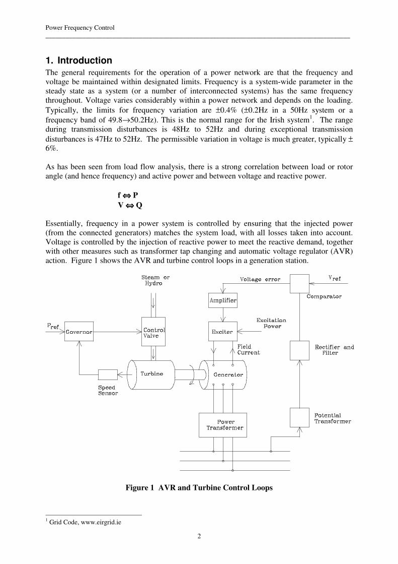
Essentially, frequency in a power system is controlled by ensuring that the injected power
(from the connected generators) matches the system load, with all losses taken into account.
Voltage is controlled by the injection of reactive power to meet the reactive demand, together
with other measures such as transformer tap changing and automatic voltage regulator (AVR)
action. Figure 1 shows the AVR and turbine control loops in a generation station.
Figure 1 AVR and Turbine Control Loops
1 Grid Code, www.eirgrid.ie
Power Frequency Control
___________________________________________________________________________________________
3
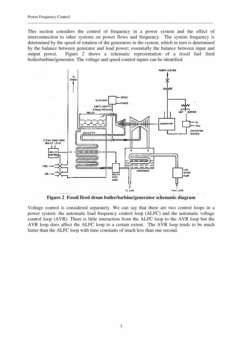
This section considers the control of frequency in a power system and the effect of
interconnection to other systems on power flows and frequency. The system frequency is
determined by the speed of rotation of the generators in the system, which in turn is determined
by the balance between generator and load power; essentially the balance between input and
output power. Figure 2 shows a schematic representation of a fossil fuel fired
boiler/turbine/generator. The voltage and speed control inputs can be identified.
Figure 2 Fossil fired drum boiler/turbine/generator schematic diagram
Voltage control is considered separately. We can say that there are two control loops in a
power system: the automatic load frequency control loop (ALFC) and the automatic voltage
control loop (AVR). There is little interaction from the ALFC loop to the AVR loop but the
AVR loop does affect the ALFC loop to a certain extent. The AVR loop tends to be much
faster than the ALFC loop with time constants of much less than one second.
Power Frequency Control
___________________________________________________________________________________________
4
Automatic
Generation Control
Turbine/Generator
Intertia
Electrical System
(a) Generators
(b) Networks
(c) Loads
Governor
Speed Changer
Speed
Governor
Speed Control
Mechanism
Governor-Controlled
Valves or Gates
Turbine
Assigned
Unit
Generation
Interchange Power
Frequency
Turbine and Energy System Speed-Governing System
Angle
Speed
Electrical
Power
Mechanical
Power
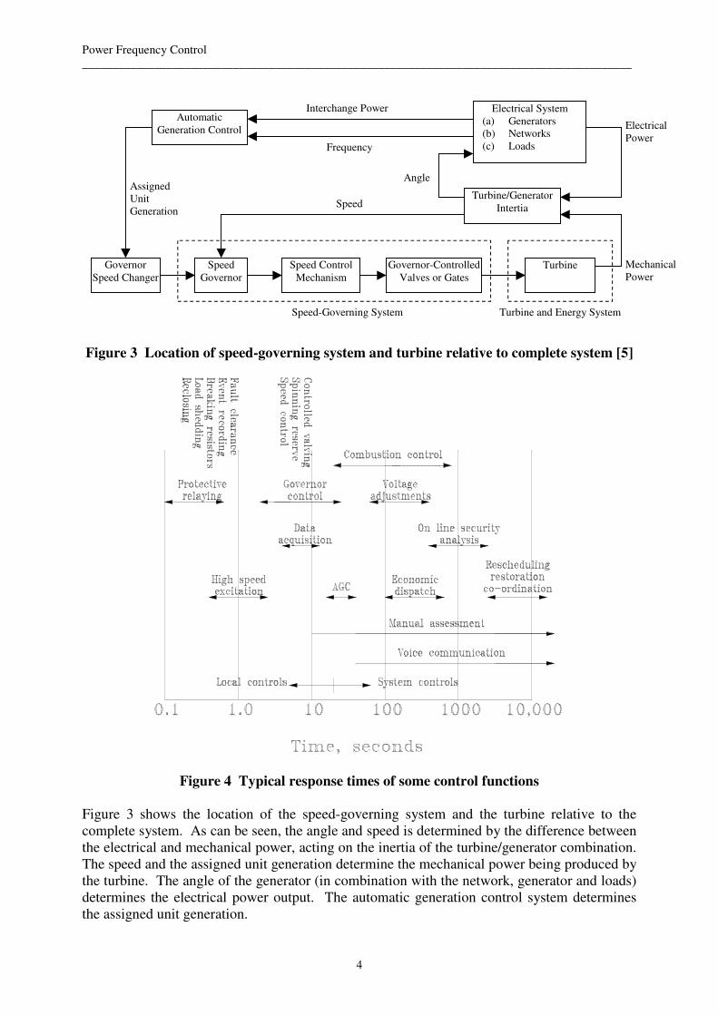
Figure 3 Location of speed-governing system and turbine relative to complete system [5]
Figure 4 Typical response times of some control functions
Figure 3 shows the location of the speed-governing system and the turbine relative to the
complete system. As can be seen, the angle and speed is determined by the difference between
the electrical and mechanical power, acting on the inertia of the turbine/generator combination.
The speed and the assigned unit generation determine the mechanical power being produced by
the turbine. The angle of the generator (in combination with the network, generator and loads)
determines the electrical power output. The automatic generation control system determines
the assigned unit generation.
Power Frequency Control
___________________________________________________________________________________________
5
Figure 4 shows the typical response times of some control functions within the power network.
The high-speed excitation and governing control functions can be identified on the left of the
diagram with response times between 1 and 10 seconds. The response times to system faults
by protection systems will be faster than this characteristic time in the range of multiples of
power cycles, up to 0.1 second.
2. Small Signal Analysis of Power Systems
Analysis of power networks can be divided into small-signal and large-signal analysis. For the
time-domain analysis of events, such as major faults where voltages can change by up to
100%, large-signal analysis is required. For small changes, where the response can be
considered linear over the typical range, small-signal or linear analysis can be used. Hence the
Laplace transform can be used to consider the time domain and frequency domain response of
such linear systems. Power frequency control in power systems is usually investigated using
linear or small-signal methods.
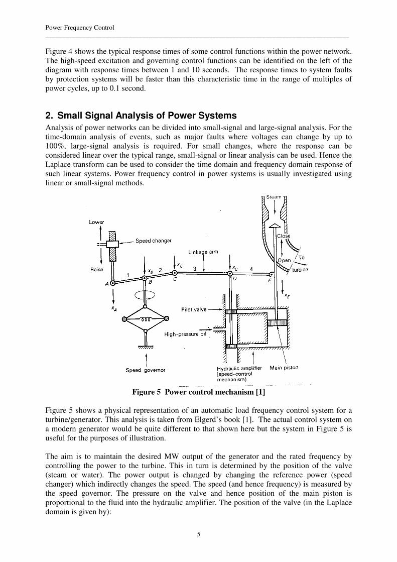
Figure 5 Power control mechanism [1]
Figure 5 shows a physical representation of an automatic load frequency control system for a
turbine/generator. This analysis is taken from Elgerd’s book [1]. The actual control system on
a modern generator would be quite different to that shown here but the system in Figure 5 is
useful for the purposes of illustration.
The aim is to maintain the desired MW output of the generator and the rated frequency by
controlling the power to the turbine. This in turn is determined by the position of the valve
(steam or water). The power output is changed by changing the reference power (speed
changer) which indirectly changes the speed. The speed (and hence frequency) is measured by
the speed governor. The pressure on the valve and hence position of the main piston is
proportional to the fluid into the hydraulic amplifier. The position of the valve (in the Laplace
domain is given by):
Power Frequency Control
___________________________________________________________________________________________
6
∆−∆
+=∆ )(
1)(
1)( sF
RsP
sT
Ksx C
G
Ge (2.1)
R is in Hz/MW and is referred to the regulation or droop. )(sPref∆ is the Laplace transform of
the change in the reference power setting and )(sF∆ is the change in the frequency. We have a
relationship between the power into (or piston position) the turbine and the reference power
and the frequency. We now require the transfer function for the turbine relating the power in to
the mechanical power out. Typically, the following transfer functions are used for turbines:
T
T
e
TT
sT
K
sx
sPsG
+=
∆
∆=
1)(
)()( Steam turbine, no reheat (2.2)
+
+
+=
RH
RH
T
TT
sT
Ts
sT
KsG
1
1
1)(
αSteam turbine, with reheat (2.3)
W
WTT
sT
sTKsG
+
−=
1
21)( Hydro (2.4)
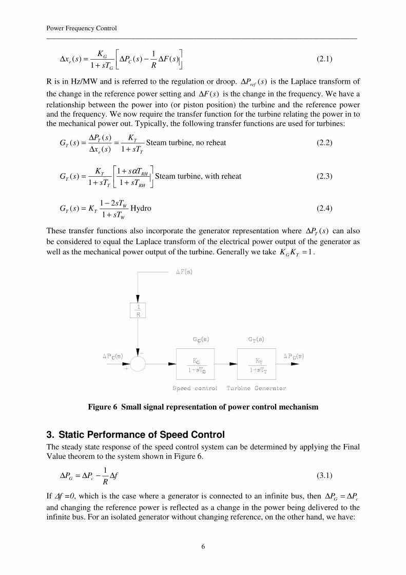
These transfer functions also incorporate the generator representation where )(sPT∆ can also
be considered to equal the Laplace transform of the electrical power output of the generator as
well as the mechanical power output of the turbine. Generally we take 1=TG KK .
Figure 6 Small signal representation of power control mechanism
3. Static Performance of Speed Control
The steady state response of the speed control system can be determined by applying the Final
Value theorem to the system shown in Figure 6.
fR
PP cG ∆−∆=∆1
(3.1)
If ∆f =0, which is the case where a generator is connected to an infinite bus, then cG PP ∆=∆
and changing the reference power is reflected as a change in the power being delivered to the
infinite bus. For an isolated generator without changing reference, on the other hand, we have:

Power Frequency Control
___________________________________________________________________________________________
7
fR
PG ∆−=∆1
(3.2)
and an increase in output power is reflected as a drop in frequency. This drop in frequency is
determined by the droop characteristic R. R is a measure of how responsive the speed
controller is to changes in frequency and is measured in Hz/MW or more usually Hz/pu MW or
%Hz/pu MW. For example, 4% droop means 2Hz/pu MW for a 50Hz system. With changes in
both reference power output and frequency, we have a family of curves as shown in Figure 7.
Figure 7 Static speed control response
If we have two generators rated at 50MW and 500MW respectively connected to a common
bus and each are at half loading, then a change in the load of 110MW results in a frequency
drop to 49.6Hz. The regulation can be calculated as follows:
R Hz MW
R Hz MW
1
2
0 4
100 04
0 4
1000 004
= =
= =
.. /
.. /
(Small unit)
(Large unit )
which gives the correct distribution of 1:10 between the machines. The regulation can be
expressed as follows:
R Hz MW
R Hz MW
1
2
0 04 0 0450
50
0 004 0 004500
50
= =
= =
. / .
. / .
pu Hz / pu MW = 4.0 %Hz / pu MW
pu Hz / pu MW = 4.0 %Hz / pu MW
and for correct distribution of load, R R1 2= when expressed as %Hz/pu MW.

Power Frequency Control
___________________________________________________________________________________________
8
4. The Power System Model
To close the ALFC loop, we now require a model for the power system. In other words, we
need a representation of the dynamic relationship between the changes in the system frequency
and the changes in demand power and the output of the generators. This allows us to
investigate how the changes in load will affect the frequency.
Initially, we identify the following, pre-disturbance operating condition:
f 0 - initial frequency
Wkin
0 - initial kinetic energy
∆PG = 0
∆PD = 0
With changes in the system frequency, there are changes in the kinetic energy of the rotating
machinery:
2
0
0
=
f
fWW kinkin (4.1)
The change in power which accompanies this change in energy is given by:
( ) fD+W
demandcustomer in change -output generator in change
kin ∆=
=∆−∆
dt
d
PP DG
(4.2)
where f
PD D
∂
∂= is the change in system demand due to a change in frequency and is assumed
positive. The frequency can be described in terms of the initial frequency and the change in
frequency:
fff ∆+= 0 (4.3)
and therefore:
∆+≈
∆+
∆+=
∆+=
0
0
2
00
0
2
0
00
21
21
f
fW
f
f
f
fW
f
ffWW
kin
kin
kinkin
(4.4)
[ ] fDfdt
d
f
WPP kin
DG ∆+∆=∆−∆0
02 (4.5)
The kinetic energy can be described in terms of the inertia constant H where
)seconds( MWrated
energy kinetic=
×==
MW
sMWH

Power Frequency Control
___________________________________________________________________________________________
9
In terms of per unit we have:
fDdt
fd
f
HPP DpuGpu ∆+
∆=∆−∆
0
2 (4.6)
If we take the Laplace transform of this equation, and dropping the pu notation, we have:
)()(2
)()(0
sFDsFsf
HsPsP DG ∆+∆=∆−∆ (4.7)
or
[ ]
P
PP
DGP
sT
KsG
sPsPsGsF
+=
∆−∆=∆
1)(
)()()()(
(4.8)
DK
Df
HT
P
P
1
20
=
=
PK relates the change in power to the change in frequency. The static performance of the
power system is given by:
[ ]DGP PPKf ∆−∆=∆ (4.9)
Figure 8 Single control area
The combined turbine/generator/speed control and power system model is shown in Figure 8
above. The combined transfer function, relating changes in frequency to changes in the
reference power and to changes in the power demand in the system is given by:
D
TGP
PC
TGP
TGP P
GGGR
GP
GGGR
GGGF ∆
+
−∆
+
=∆1
11
1
(4.10)
If CP∆ =0 (no change in reference power) and if a step change occurs in the load demand:

Power Frequency Control
___________________________________________________________________________________________
10
s
MsPD =∆ )(
then the change in frequency is given by:
s
M
GGGR
GF
TGP
P
11+
−=∆ (4.11)
0 1 2 3 4 5 6 7 8 9 100
0.05
0.1
0.15
0.2
0.25
0.3
0.35
0.4
0.45
0.5
time,seconds
change in f
requency,
Hz
R=4%
R=20%
Figure 9 Step response of system, ∆PD = -0.05 p.u.
Figure 9 shows the response in system frequency for two different values of regulation R. The
step load change is -0.05 pu (decrease in load) in both cases. The steady-state frequency
change can be determined by applying the Final Value Theorem to the above equation:
β
M
RD
M
MRK
K
sFsf
p
P
stL
−=
+
−=
+
−=
∆=∆→∞→
/1
/1
)(0
(4.12)
where RD /1+=β and is called the Area Frequency Response Characteristic (AFRC).
Considering the case shown in Figure 9 above where puPD 05.0−=∆ and D =0.01 puMW/Hz,
for
R = 4%, β = 0.01+0.5 = 0.51, ∆f=0.098Hz
R = 20%, β = 0.01+0.1 = 0.11, ∆f=0.454Hz

Power Frequency Control
___________________________________________________________________________________________
11
For R=∞, β=0.01 and the change in frequency is 5Hz. In this case, the original change in
demand is completely balanced by an equal and opposite drop in system demand because of
the drop in frequency and there is no increase in output power.
We can identify three sources of power in the system to meet an increase in demand which is
accompanied by a frequency drop:
a) The change in kinetic energy of the rotating machinery. As the frequency drops,
energy is released by the machines and this provides a short-term source of power.
b) Increased generation because of the speed control loop.
c) A reduction in load due to a decrease in frequency.
Often, the time constants GT and TT are set to zero to simplify the analysis as this reduces the
system to a first order model. The steady-state values remain unchanged but the dynamic
behaviour changes greatly.
0 1 2 3 4 5 6 7 8 9 100
0.02
0.04
0.06
0.08
0.1
0.12
0.14
0.16
time,seconds
change in f
requency,
Hz
Tt=0.1,Tt=0.5
Tt=Tg=0
Figure 10 Effect of time constants
5. The Reset Loop
With the speed governor action only, there is a finite error in the frequency when the system
settles down again to the steady-state and is given by:
β
Mf
−=∆ (5.1)
Therefore, integral control action is added which changes the reference power level and returns
the system frequency error to zero.
∫∆−=∆ fdtKP IC (5.2)
Power Frequency Control
___________________________________________________________________________________________
12
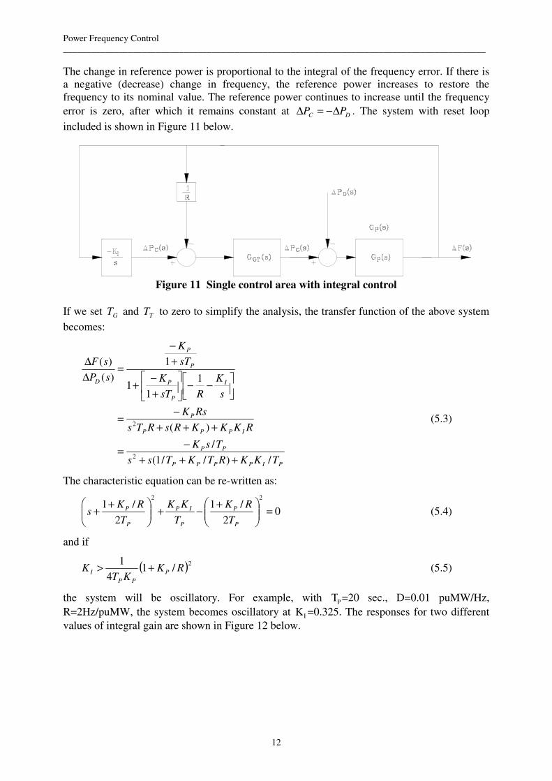
The change in reference power is proportional to the integral of the frequency error. If there is
a negative (decrease) change in frequency, the reference power increases to restore the
frequency to its nominal value. The reference power continues to increase until the frequency
error is zero, after which it remains constant at DC PP ∆−=∆ . The system with reset loop
included is shown in Figure 11 below.
Figure 11 Single control area with integral control
If we set GT and TT to zero to simplify the analysis, the transfer function of the above system
becomes:
PIPPPP
PP
IPPP
P
I
P
P
P
P
D
TKKRTKTss
TsK
RKKKRsRTs
RsK
s
K
RsT
K
sT
K
sP
sF
/)//1(
/
)(
1
11
1
)(
)(
2
2
+++
−=
+++
−=
−−
+
−+
+
−
=∆
∆
(5.3)
The characteristic equation can be re-written as:
02
/1
2
/122
=
+−+
++
P
P
P
IP
P
P
T
RK
T
KK
T
RKs (5.4)
and if
( )2/1
4
1RK
KTK P
PP
I +> (5.5)
the system will be oscillatory. For example, with TP=20 sec., D=0.01 puMW/Hz,
R=2Hz/puMW, the system becomes oscillatory at KI =0.325. The responses for two different
values of integral gain are shown in Figure 12 below.

Power Frequency Control
___________________________________________________________________________________________
13
0 1 2 3 4 5 6 7 8 9 10-0.01
0
0.01
0.02
0.03
0.04
0.05
0.06
0.07
0.08
time,seconds
change in f
requency,
Hz
Ki=0.3
Ki=0.7
Figure 12 Effect of integral control gain
A higher gain in the reset loop will lead to a faster response but will also cause oscillations and,
if this gain exceeds a critical value, cause instability.
For clocks which are controlled by the system frequency, every change in the frequency (even
transient changes) will cause time errors. The error introduced over a time T can be expressed
as:
∫∆=T
e fdtf
t0
0
1 (5.6)
Problem: By applying the Final Value Theorem, calculate the time error due to a change in demand of
0.05pu in the system shown in Figure 12 above if the integral control gain is 0.7. Suggest how
this error might be subsequently set to zero.

Power Frequency Control
___________________________________________________________________________________________
14
6. Pool Operation
We have considered the operation of a single, isolated power system. In situations where a
number of systems are connected by interties, then there are advantages to be gained for the
overall system both in terms of the normal operation and for emergency conditions.
Interconnected systems can provide support for each other in the event of a sudden application
of a large load or fault condition. A combined system will lead to more economic operation.
The rules of pool operation are usually such that each area carries its own load except under
mutually agreed circumstances. Because a number of systems connected together represents a
much larges system, the impact of any load change in terms of frequency change will be much
smaller than it would be on single system. Figure 13 shows the response of a single area and
Figure 14 shows the response of a two area system to the same load change.
0 1 2 3 4 5 6 7 8 9 100
0.02
0.04
0.06
0.08
0.1
0.12
0.14
0.16
time,seconds
change in
fre
que
ncy,
Hz
0 1 2 3 4 5 6 7 8 9 100
0.02
0.04
0.06
0.08
0.1
0.12
0.14
Area 1
Area 2
time,seconds
change in
fre
que
ncy,
Hz
Figure 13 Response of single area Figure 14 Response of two areas
The power transfer over a connection between two areas is given by:
)sin( 21
21
12 δδ −=X
VVP (6.1)
where P12 is the power flow from area 1 to area 2, V1 1∠δ and V2 2∠δ are the voltage at each end
of the connecting line and X is the reactance of that line. Initially, the operating point is given
by:
)sin( 0
2
0
1
0
2
0
10
12 δδ −=X
VVP (6.2)
and small deviations from this point are given by:
))(cos( 21
0
2
0
1
0
2
0
1
12 δδδδ ∆−∆−=∆X
VVP (6.3)
where the any changes in the voltage magnitudes in each system are neglected. This equation
may be written as:
)cos(
)(
0
2
0
1
0
2
0
10
12
21
0
1212
δδ
δδ
−=
∆−∆=∆
X
VVT
TP
(6.4)
0
12T is called the synchronising coefficient and is determined by the operating point. The
change in frequency is given by:
Power Frequency Control
___________________________________________________________________________________________
15
dt
d
dt
df
)(
2
1)(
2
1 0 δ
πδδ
π
∆=
∆+=∆ (6.5)
∫∆=∆t
fdt0
2πδ (6.6)
and therefore
)(20
2
0
1
0
1212 ∫∫ ∆−∆=∆tt
dtfdtfTP π (6.7)
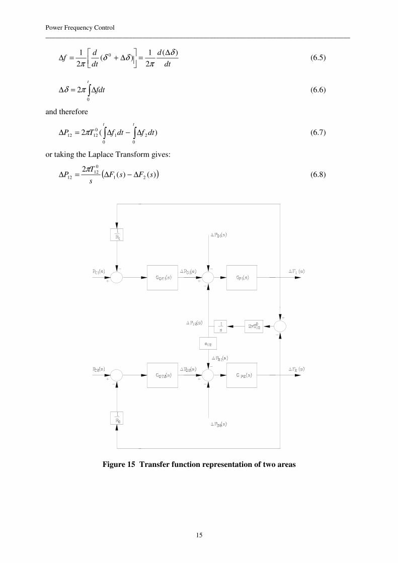
or taking the Laplace Transform gives:
( ))()(2
21
0
12
12 sFsFs
TP ∆−∆=∆
π (6.8)
Figure 15 Transfer function representation of two areas
Power Frequency Control
___________________________________________________________________________________________
16
Figure 15 above shows the representation of a two-area system with the interconnection
between the areas included. The frequency deviation for areas 1 and 2 are given by:
( )
( )12122
22
2
2
121
11
1
1
/)(1
)()(
/)(1
)()(
PaPRsG
sGsF
PPRsG
sGsF
D
P
P
D
P
P
∆+∆+
−=∆
∆+∆+
−=∆
(6.9)
( ))()(2
21
0
12
12 sFsFs
TP ∆−∆=∆
π (6.10)
2 Area BasePower
1 Area BasePower 12 −=a (6.11)
Combining these three equations allows us to calculate the frequency deviation for each area
and the power transfer between the areas. Consider a change in load of M1 in area 1 and a
change in load of M2 in area 2. By the Final Value Theorem, we can show that the steady-state
power flow between these areas as a result of these load changes is given by:
2112
1221
12ββ
ββ
+−
−=∆
a
MMP (6.12)
where: 222
111
/1
/1
RD
RD
+=
+=
β
β
and the frequency deviations are given by:
+−
+−=∆
+−
+−=∆
2112
21
2
2112
21
1
ββ
ββ
a
MMf
a
MMf
(6.13)
Obviously since the areas are interconnected, they will both settle down to the same frequency
deviation.
Problem: Two areas connected by a transmission line and have the following values:
Area 1: R=4%, TP=20sec, D=0.01, ∆PD=-0.05
Area 2: R=8%, TP=20sec, D=0.05, ∆PD=0.03
Calculate the eventual steady-state power flow between the areas and the frequency deviation.

Power Frequency Control
___________________________________________________________________________________________
17
0 2 4 6 8 10 12 14 16 18 20-0.1
-0.05
0
0.05
0.1
0.15
0.2
0.25
time,seconds
change in f
requency,
Hz
Area A
Area B
Figure 16 Response of areas without interconnection
0 2 4 6 8 10 12 14 16 18 20-0.04
-0.02
0
0.02
0.04
0.06
0.08
0.1
0.12
0.14
time,seconds
change in f
requency,
Hz
Area A
Area B
0 2 4 6 8 10 12 14 16 18 200
0.005
0.01
0.015
0.02
0.025
0.03
0.035
0.04
0.045
time,seconds
pow
er
flow
, p.u
.
Figure 17 Response of areas with interconnection, frequency and power
Figure 16 above shows the response of these systems without an interconnection. The
frequency changes are different as there is no connection. The situation with an interconnection
is shown in Figure 17. Obviously, with this system, there is a finite frequency error again (the
same for both areas) and an unscheduled power flow between the areas. As before, we wish to
return both the change in frequency and the power to zero and this is accomplished by integral
control action.
The area control error (ACE) consists of components of the power error and the frequency
error and is given by:
22212
11121
fBPACE
fBPACE
∆+∆=
∆+∆= (6.14)
and B is the frequency bias parameter. The changes in reference power now become:
Power Frequency Control
___________________________________________________________________________________________
18
( )
( )dtfBPKP
dtfBPKP
IC
IC
∫
∫∆+∆−=∆
∆+∆−=∆
222122
111211
(6.15)
and taking the Laplace Transform:
( )
( ))()()(
)()()(
2221
2
2
1112
1
1
sFBsPs
KsP
sFBsPs
KsP
I
C
I
C
∆+∆−=∆
∆+∆−=∆
(6.16)
The static response is given by:
0
0
22122212
11211121
=∆+∆=∆+∆=
=∆+∆=∆+∆=
fBPfBPACE
fBPfBPACE (6.17)
and this condition is met for ∆f=0 and 02112 =∆=∆ PP .
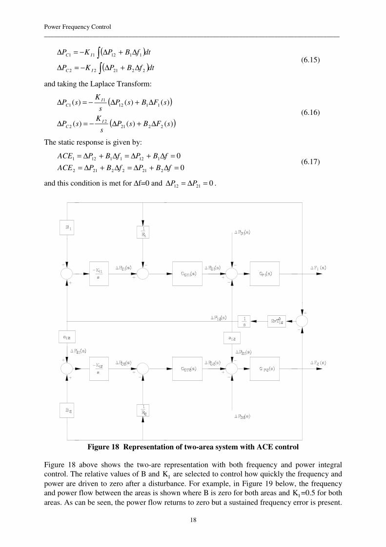
Figure 18 Representation of two-area system with ACE control
Figure 18 above shows the two-are representation with both frequency and power integral
control. The relative values of B and KI are selected to control how quickly the frequency and
power are driven to zero after a disturbance. For example, in Figure 19 below, the frequency
and power flow between the areas is shown where B is zero for both areas and KI =0.5 for both
areas. As can be seen, the power flow returns to zero but a sustained frequency error is present.

Power Frequency Control
___________________________________________________________________________________________
19
On the other hand, if we make B=40 for both areas and if KI is very small, then as can be seen
in Figure 20, the power flow is very slow in returning to zero even though the frequency error
rapidly dies away. Figure 21 shows a reasonable compromise between these two extremes.
0 2 4 6 8 10 12 14 16 18 20-0.04
-0.02
0
0.02
0.04
0.06
0.08
0.1
0.12
0.14
time,seconds
chan
ge in f
req
uency
, H
z
Area 1
Area 2
0 2 4 6 8 10 12 14 16 18 20
-0.02
-0.01
0
0.01
0.02
0.03
0.04
time,seconds
pow
er
flow
, p
.u.
Figure 19 Power integral control only
0 2 4 6 8 10 12 14 16 18 20-0.1
-0.05
0
0.05
0.1
0.15
time,seconds
chang
e in f
requenc
y,
Hz
Area 1
Area 2
0 2 4 6 8 10 12 14 16 18 200
0.005
0.01
0.015
0.02
0.025
0.03
time,seconds
pow
er
flow
, p.u
.
Figure 20 Frequency integral control only
0 2 4 6 8 10 12 14 16 18 20-0.1
-0.05
0
0.05
0.1
0.15
time,seconds
change in f
requency,
Hz
Area 1
Area 2
0 2 4 6 8 10 12 14 16 18 20-0.01
-0.005
0
0.005
0.01
0.015
0.02
0.025
0.03
time,seconds
pow
er
flow
, p.u
.
Figure 21 Combined Frequency and power integral control
7. State-Space Representation of a Two Area System
For analysis of larger linear systems, the state-space representation is used. This allows for a
more convenient approach to analysis and controller design. This section looks at the state-
space representation of the two-area system is developed.
Power Frequency Control
___________________________________________________________________________________________
20
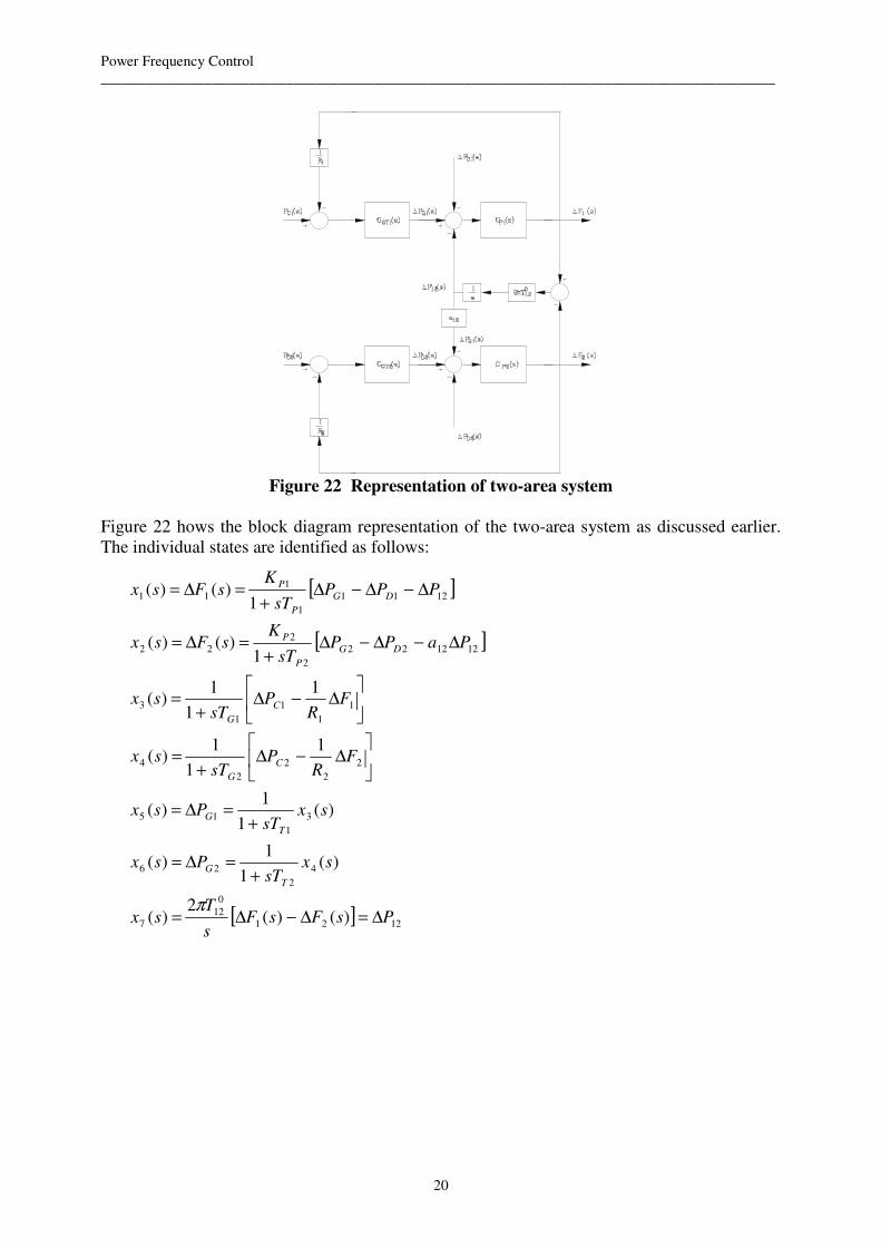
Figure 22 Representation of two-area system
Figure 22 hows the block diagram representation of the two-area system as discussed earlier.
The individual states are identified as follows:
[ ]
[ ]
[ ] 1221
0
12
7
4
2
26
3
1
15
2
2
2
2
4
1
1
1
1
3
121222
2
2
22
1211
1
1
11
)()(2
)(
)(1
1)(
)(1
1)(
1
1
1)(
1
1
1)(
1)()(
1)()(
PsFsFs
Tsx
sxsT
Psx
sxsT
Psx
FR
PsT
sx
FR
PsT
sx
PaPPsT
KsFsx
PPPsT
KsFsx
T
G
T
G
C
G
C
G
DG
P
P
DG
P
P
∆=∆−∆=
+=∆=
+=∆=
∆−∆
+=
∆−∆
+=
∆−∆−∆+
=∆=
∆−∆−∆+
=∆=
π

Power Frequency Control
___________________________________________________________________________________________
21
and the corresponding differential equations are given by:
[ ]21
0
127
.
6
2
4
2
6
.
5
1
3
1
5
.
2
2
2
22
4
2
4
.
1
1
1
11
3
1
3
.
2
2
2
7
2
2
126
2
2
2
2
2
.
1
1
1
7
1
1
5
1
1
1
1
1
.
2
11
11
111
111
1
1
xxTx
xT
xT
x
xT
xT
x
PT
xTR
xT
x
PT
xTR
xT
x
PT
Kx
T
Kax
T
Kx
Tx
PT
Kx
T
Kx
T
Kx
Tx
TT
TT
C
GGG
C
GGG
D
P
P
P
P
P
P
P
D
P
P
P
P
P
P
P
−=
−=
−=
∆+−−=
∆+−−=
∆−−+−=
∆−−+−=
π
These equations can we written in conventional state-space form as follows:
pBuAxx Γ++=.
(7.1)
where:
=
7
6
5
4
3
2
1
x
x
x
x
x
x
x
x ;
∆
∆=
=
2
1
2
1
C
C
P
P
u
uu ;
∆
∆=
=
2
1
2
1
D
D
P
P
p
pp
−
−
−
−−
−−
−−
−−
=
0000022
01
01
000
001
01
00
0001
01
0
00001
01
0001
0
00001
0
12
0
12
22
11
222
111
2
2
12
2
2
2
1
1
1
1
1
TT
TT
TT
TTR
TTR
T
Ka
T
K
T
T
K
T
K
T
A
TT
TT
GG
GG
P
P
P
P
P
P
P
P
P
P
ππ

Power Frequency Control
___________________________________________________________________________________________
22
=
00
00
00
10
01
00
00
2
1
G
G
T
T
B ;
−
−
=Γ
00
00
00
00
00
0
0
2
2
1
1
G
P
G
P
T
K
T
K
Figure 23 Two-area system with ACE
If ACE control is implemented, as shown in Figure 23, then the state-space representation is
augmented to include the reference power for each area ∆PC1 and ∆PC2 as states and becomes:
[ ]
[ ] 2121222
2
9
11211
1
8
)(
)(
C
I
C
I
PPaFBs
Ksx
PPFBs
Ksx
∆=∆+∆−=
∆=∆+∆−=
and these changes are made to the differential equations:
72122229
.
711118
.
9
2
2
22
4
2
4
.
8
1
1
11
3
1
3
.
111
111
xKaxBKx
xKxBKx
xT
xTR
xT
x
xT
xTR
xT
x
II
II
GGG
GGG
−−=
−−=
+−−=
+−−=
and the state-space representation becomes:
Power Frequency Control
___________________________________________________________________________________________
23
pAxx Γ+=.
(7.2)
where:
=
9
8
7
6
5
4
3
2
1
x
x
x
x
x
x
x
x
x
x
−
−
=Γ
00
00
00
00
00
00
00
0
0
2
2
1
1
G
P
G
P
T
K
T
K
−−
−−
−
−
−
−−
−−
−−
−−
=
0000000
0000000
000000022
0001
01
000
00001
01
00
10000
10
10
01
00001
01
000001
0
0000001
21222
111
0
12
0
12
22
11
2222
1111
2
2
12
2
2
2
1
1
1
1
1
II
II
TT
TT
GGG
GGG
P
P
P
P
P
P
P
P
P
P
KaBK
KBK
TT
TT
TT
TTTR
TTTR
T
Ka
T
K
T
T
K
T
K
T
A
ππ
References
1. O.I. Elgerd, Electric energy systems theory: An Introduction, McGraw Hill, 1983
2. C.A. Gross, Power systems analysis, Wiley, 1986
3. B.M. Weedy, Electric power systems, Wiley, 1972
4. W.D. Stevenson, Elements of power system analysis, McGraw Hill, 1986, Chap. 8
5. Dynamic models for steam and hydro turbines in power system studies, IEEE Committee
report, IEEE Trans., Vol. PAS-92, No. 6, Nov./Dec. 1973
6. T.M. Athay, Generation scheduling and control, Proc. IEEE, Vol. 75, No.12, 1987
7. A.J. Wood and B.F. Wollenburg, Power generation, operation, and control, Wiley, 1984
8. O.I. Elgerd and C.E. Fosha, Optimum megawatt-frequency control of multiarea electric
energy systems, IEEE Trans., PAS-89, No. 4, April 1970, p 556
9. P. Kundur, Power System Strability and Control, McGraw-Hill, 1994, Chap. 11
Michael F. Conlon
September 2003
![Power over Ethernet Commands - Cisco - Global …show switch power inline [{consumed-power |nominal-power |power-limit-mode}] SyntaxDescription consumed-power Displaystotalconsumedpower](https://cdn.vdocuments.us/doc/165x107/5ecaf5925fef0574637f1fb1/power-over-ethernet-commands-cisco-global-show-switch-power-inline-consumed-power.jpg)


