
Universite Libre de Bruxelles
Ecole Polytechnique de Bruxelles
CODE - Computers and Decision Engineering
IRIDIA - Institut de Recherches Interdisciplinaires
et de Developpements en Intelligence Artificielle
Population-based Heuristic Algorithms
for Continuous and Mixed
Discrete-Continuous Optimization Problems
Tianjun LIAO
Promoteur:
Prof. Marco DORIGO
Co-promoteur:
Dr. Thomas STUTZLE
These presentee a la Ecole Polytechnique de Bruxelles de l’Universite Libre de Bruxelles en
vue de l’obtention du titre de Docteur en Sciences de l’Ingenieur.
Annee Academique 2012-2013

ii
Summary
Continuous optimization problems are optimization problems where all variables
have a domain that typically is a subset of the real numbers; mixed discrete-
continuous optimization problems have additionally other types of variables, so
that some variables are continuous and others are on an ordinal or categorical
scale. Continuous and mixed discrete-continuous problems have a wide range
of applications in disciplines such as computer science, mechanical or electrical
engineering, economics and bioinformatics. These problems are also often hard to
solve due to their inherent difficulties such as a large number of variables, many
local optima or other factors making problems hard. Therefore, in this thesis our
focus is on the design, engineering and configuration of high-performing heuristic
optimization algorithms.
We tackle continuous and mixed discrete-continuous optimization problems
with two classes of population-based heuristic algorithms, ant colony optimization
(ACO) algorithms and evolution strategies. In a nutshell, the main contributions
of this thesis are that (i) we advance the design and engineering of ACO algo-
rithms to algorithms that are competitive or superior to recent state-of-the-art
algorithms for continuous and mixed discrete-continuous optimization problems,
(ii) we improve upon a specific state-of-the-art evolution strategy, the covariance
matrix adaptation evolution strategy (CMA-ES), and (iii) we extend CMA-ES to
tackle mixed discrete-continuous optimization problems.
More in detail, we propose a unified ant colony optimization (ACO) framework
for continuous optimization (UACOR). This framework synthesizes algorithmic
components of two ACO algorithms that have been proposed in the literature
and an incremental ACO algorithm with local search for continuous optimization,
which we have proposed during my doctoral research. The design of UACOR
allows the usage of automatic algorithm configuration techniques to automatically
derive new, high-performing ACO algorithms for continuous optimization. We also
propose iCMAES-ILS, a hybrid algorithm that loosely couples IPOP-CMA-ES, a
CMA-ES variant that uses a restart schema coupled with an increasing population
iii

size, and a new iterated local search (ILS) algorithm for continuous optimization.
The hybrid algorithm consists of an initial competition phase, in which IPOP-
CMA-ES and the ILS algorithm compete for further deployment during a second
phase. A cooperative aspect of the hybrid algorithm is implemented in the form
of some limited information exchange from IPOP-CMA-ES to the ILS algorithm
during the initial phase. Experimental studies on recent benchmark functions
suites show that UACOR and iCMAES-ILS are competitive or superior to other
state-of-the-art algorithms.
To tackle mixed discrete-continuous optimization problems, we extend ACOMV
and propose CESMV, an ant colony optimization algorithm and a covariance ma-
trix adaptation evolution strategy, respectively. In ACOMV and CESMV, the de-
cision variables of an optimization problem can be declared as continuous, ordinal,
or categorical, which allows the algorithm to treat them adequately. ACOMV and
CESMV include three solution generation mechanisms: a continuous optimization
mechanism, a continuous relaxation mechanism for ordinal variables, and a cate-
gorical optimization mechanism for categorical variables. Together, these mecha-
nisms allow ACOMV and CESMV to tackle mixed variable optimization problems.
We also propose a set of artificial, mixed-variable benchmark functions, which can
simulate discrete variables as ordered or categorical. We use them to automati-
cally tune ACOMV and CESMV’s parameters and benchmark their performance.
Finally we test ACOMV and CESMV on various real-world continuous and mixed-
variable engineering optimization problems. Comparisons with results from the
literature demonstrate the effectiveness and robustness of ACOMV and CESMV
on mixed-variable optimization problems.
Apart from these main contributions, during my doctoral research I have ac-
complished a number of additional contributions, which concern (i) a note on the
bound constraints handling for the CEC’05 benchmark set, (ii) computational re-
sults for an automatically tuned IPOP-CMA-ES on the CEC’05 benchmark set and
(iii) a study of artificial bee colonies for continuous optimization. These additional
contributions are to be found in the appendix to this thesis.
iv
Acknowledgements
I express my deep gratitude to my supervisors, Prof. Marco Dorigo and Dr. Thomas
Stutzle for giving me the chance to do research at IRIDIA. I thank them for their
supervision that had a great influence not only on this thesis but also on my
attitude to work and life. They are very professional. I feel very lucky to work
with them. They are deeply engraved in my mind.
I first contacted Marco by email on January 6, 2009. He swiftly replied me with
interest. From then on, he fully supported me in many aspects including invitation
letter, fellowship, inscription and so on. He was patient and always efficiently
replied me in everything I proposed to him. Finally, on November 11, 2009, I
started my PhD research in IRIDIA. Marco is not only the “rider on a swarm”
as reported by magazine The Economist but also a very nice PhD supervisor. I
like his smile, his straightforward and serious attitude to work, and especially his
clear-cut, short sentences. I am proud of him. I greatly appreciate his careful
proof reading of my articles and thesis. We cooperate well in many aspects with
a tacit mutual understanding.
I thank my co-supervisor, Dr. Thomas Stutzle, a super kind person. He plays a
crucial role in my research. His charisma and his spirit of scientific research deeply
affected me. He is a fantastic scientist and PhD supervisor. In the field of heuristic
optimization, his knowledge is just like the ocean, never a rim. He soaks up new
subjects as a sponge soaks up water. His comments are always very helpful. He
delivers positive energy and passion. His passion, expertise and critical thought
promoted each of my research activities. We work together almost every day, on
each of my research articles. We exchange opinions and share what we like and
what we do not. I enjoy much working with him. In fact, he is more like my
colleague and friend. As writing here, my mind has flashed back to many scenes
of the past. I do not want to continue because those words sound that I am going
to leave. In fact, I expect working longer with him, even a life time.
I express my appreciation to Prof. Yuejin Tan, Associate Prof. Kewei Yang and
their related departments. They gave me the chance to study abroad and helped
v

me to apply for a fellowship from the China Scholarship Council.
Special thanks to the co-authors in my publications and fellow IRIDIAns. All
of them, Anthony Antoun, Dogan Aydın, Prasanna Balaprakash, Hugues Bersini,
Leonardo Bezerra, Stefano Benedettini, Saifullah bin Hussin, Mauro Birattari,
Manuele Brambilla, Arne Brutschy, Alexandre Campo, Sara Ceschia, Muriel De-
creton, Antal Decugniere, Jeremie Dubois-Lacoste, Eliseo Ferrante, Gianpiero
Francesca, Matteo Gagliolo, Lorenzo Garattoni , Kiyohiko Hattori, Stefanie
Kritzinger, Benjamin Lacroix, Manuel Lopez-Ibanez, Renaud Lenne, Dhanan-
jay Ipparthi, Bruno Marchal, Franco Mascia, Nithin Mathews, Marie-Eleonore
Marmion, Roman Miletitch, Marco A. Montes de Oca, Daniel Molina, Prospero
C. Naval, Rehan O’Grady, Sabrina Oliveira, Michele Pace, Paola Pellegrini, Leslie
Perez Caceres, Carlo Pinciroli, Giovanni Pini, Carlotta Piscopo, Gaetan Pode-
vijn, Andreagiovanni Reina, Andrea Roli, Francesco Sambo, Francisco C. Santos,
Alexander Scheidler, Krzysztof Socha, Touraj Soleymani, Alessandro Stranieri,
Wenjie Sun, Vito Trianni, Roberto Tavares, Ali Emre Turgut, Gabriele Valen-
tini and Zhi Yuan helped me in different ways throughout these years. I also
thank Prof. Hugues Bersini, co-director of IRIDIA with Prof. Marco Dorigo, for
making IRIDIA such an enjoyable research lab. I also want to thank Prof. Marc
Schoenauer from INRIA Saclay-Ile-de-France, Prof. Bernard Fortz, Prof. Hugues
Bersini, Dr. Mauro Birattari and Dr. Manuel Lopez-Ibanez from Universite Libre
de Bruxelles for their useful comments.
My special appreciation goes to my parents, Yingmin Liao and Xiaoou Xu, and
Miss Jinyu Zhang. I thank very much for their love and care. I also thank all my
dear friends. They gave me very much support during the time I lived in Brussels.
This work was supported by the E-SWARM project, Engineering Swarm
Intelligence Systems, funded by the European Union’s Seventh Framework
Programme (FP7/2007-2013) / ERC grant agreement nº 246939 and by the
Meta-X project, Metaheuristics for Complex Optimization Problems, funded by
the Scientific Research Directorate of the French Community of Belgium. Tianjun
Liao acknowledges a fellowship from the China Scholarship Council.
Tianjun Liao
June 18th, 2013
Brussels, Belgium.
vi

Contents
1 Introduction 1
1.1 Goal and methodology . . . . . . . . . . . . . . . . . . . . . . . . . 3
1.2 Main contributions . . . . . . . . . . . . . . . . . . . . . . . . . . . 4
1.3 Additional contributions . . . . . . . . . . . . . . . . . . . . . . . . 7
1.4 Publications . . . . . . . . . . . . . . . . . . . . . . . . . . . . . . . 8
1.4.1 International journal submissions . . . . . . . . . . . . . . . 9
1.4.2 International conferences and workshops (peer-reviewed) . . 10
1.5 Structure of the thesis . . . . . . . . . . . . . . . . . . . . . . . . . 11
2 Background 13
2.1 Continuous optimization . . . . . . . . . . . . . . . . . . . . . . . . 14
2.1.1 Local search algorithms . . . . . . . . . . . . . . . . . . . . 15
2.1.2 Metaheuristic based algorithms . . . . . . . . . . . . . . . . 18
2.1.3 Benchmark functions sets . . . . . . . . . . . . . . . . . . . 23
2.2 Mixed discrete-continuous optimization . . . . . . . . . . . . . . . . 27
2.3 Basic Algorithms . . . . . . . . . . . . . . . . . . . . . . . . . . . . 29
2.3.1 ACOR . . . . . . . . . . . . . . . . . . . . . . . . . . . . . . 29
2.3.2 CMA-ES . . . . . . . . . . . . . . . . . . . . . . . . . . . . . 31
2.4 Automatic algorithm configuration . . . . . . . . . . . . . . . . . . 34
2.4.1 Iterated F-Race . . . . . . . . . . . . . . . . . . . . . . . . . 34
2.4.2 Tuning methodology . . . . . . . . . . . . . . . . . . . . . . 35
2.5 Summary . . . . . . . . . . . . . . . . . . . . . . . . . . . . . . . . 36
3 UACOR: A unified ACO algorithm for continuous optimization 39
3.1 ACO algorithms for continuous optimization . . . . . . . . . . . . . 41
3.1.1 Algorithmic components . . . . . . . . . . . . . . . . . . . . 43
3.2 UACOR . . . . . . . . . . . . . . . . . . . . . . . . . . . . . . . . . 46
3.3 Automatic algorithm configuration . . . . . . . . . . . . . . . . . . 48
3.4 Algorithm evaluation . . . . . . . . . . . . . . . . . . . . . . . . . . 54
vii

CONTENTS
3.5 UACOR+: Re-designed UACOR . . . . . . . . . . . . . . . . . . . . 62
3.6 Summary . . . . . . . . . . . . . . . . . . . . . . . . . . . . . . . . 65
4 iCMAES-ILS: A cooperative competitive hybrid algorithm for
continuous optimization 67
4.1 iCMAES-ILS algorithm . . . . . . . . . . . . . . . . . . . . . . . . . 69
4.1.1 ILS . . . . . . . . . . . . . . . . . . . . . . . . . . . . . . . . 69
4.1.2 iCMAES-ILS . . . . . . . . . . . . . . . . . . . . . . . . . . 70
4.2 Algorithm analysis and evaluation . . . . . . . . . . . . . . . . . . . 71
4.2.1 Algorithm analysis: the role of ILS . . . . . . . . . . . . . . 72
4.2.2 Performance evaluation of iCMAES-ILS . . . . . . . . . . . 76
4.3 A tuned version of iCMAES-ILS . . . . . . . . . . . . . . . . . . . . 78
4.3.1 Automatic algorithm configuration . . . . . . . . . . . . . . 78
4.3.2 Performance evaluation of iCMAES-ILSt . . . . . . . . . . . 80
4.4 Comparisions of iCMAES-ILS and UACOR+ . . . . . . . . . . . . . 85
4.5 Summary . . . . . . . . . . . . . . . . . . . . . . . . . . . . . . . . 88
5 Mixed discrete-continuous optimization 89
5.1 Artificial mixed discrete-continuous benchmark functions . . . . . . 91
5.2 ACOMV: ACO for mixed discrete-continuous optimization problems 94
5.2.1 Algorithm analysis . . . . . . . . . . . . . . . . . . . . . . . 99
5.3 CMA-ES extensions for mixed discrete-continuous optimization . . 104
5.3.1 CES-RoundC . . . . . . . . . . . . . . . . . . . . . . . . . . 104
5.3.2 CESMV . . . . . . . . . . . . . . . . . . . . . . . . . . . . . 105
5.3.3 CES-RelayC . . . . . . . . . . . . . . . . . . . . . . . . . . . 107
5.4 Automatic tuning and performance evaluation . . . . . . . . . . . . 108
5.4.1 Automatic tuning . . . . . . . . . . . . . . . . . . . . . . . . 108
5.4.2 Performance evaluation on benchmark functions . . . . . . . 109
5.5 Application to engineering optimization problems . . . . . . . . . . 114
5.6 Summary . . . . . . . . . . . . . . . . . . . . . . . . . . . . . . . . 123
6 Summary and future work 125
6.1 Summary . . . . . . . . . . . . . . . . . . . . . . . . . . . . . . . . 125
6.2 Future work . . . . . . . . . . . . . . . . . . . . . . . . . . . . . . . 128
Appendices 131
A The results obtained by UACOR+ 131
viii

CONTENTS
B Mathematical formulation of engineering problems 141
C A note on the bound constraints handling for the CEC’05 bench-
mark set 147
C.1 Introduction . . . . . . . . . . . . . . . . . . . . . . . . . . . . . . . 147
C.2 Experiments on enforcing bound constraints . . . . . . . . . . . . . 149
C.3 The impact of bound handling on algorithm comparisons . . . . . . 150
C.4 Conclusions . . . . . . . . . . . . . . . . . . . . . . . . . . . . . . . 151
D Computational results for an automatically tuned IPOP-CMA-ES
on the CEC’05 benchmark set 155
D.1 Introduction . . . . . . . . . . . . . . . . . . . . . . . . . . . . . . . 155
D.2 Parameterized iCMA-ES . . . . . . . . . . . . . . . . . . . . . . . . 158
D.3 Experimental setup and tuning . . . . . . . . . . . . . . . . . . . . 159
D.4 Experimental study . . . . . . . . . . . . . . . . . . . . . . . . . . . 161
D.4.1 iCMA-ES-tsc vs. iCMA-ES-dp . . . . . . . . . . . . . . . . . 162
D.4.2 iCMA-ES-tsc vs. iCMA-ES-tcec . . . . . . . . . . . . . . . . 166
D.4.3 Comparison to state-of-the-art methods that exploit CMA-ES167
D.5 Additional experiments . . . . . . . . . . . . . . . . . . . . . . . . . 168
D.5.1 Comparison to other results by iCMA-ES . . . . . . . . . . . 168
D.5.2 Tuning setup . . . . . . . . . . . . . . . . . . . . . . . . . . 169
D.6 Conclusions and future work . . . . . . . . . . . . . . . . . . . . . . 171
E Artificial bee colonies for continuous optimization: Experimental
analysis and improvements 177
E.1 Introduction . . . . . . . . . . . . . . . . . . . . . . . . . . . . . . . 177
E.2 Artificial bee colony algorithm . . . . . . . . . . . . . . . . . . . . . 179
E.2.1 Original ABC algorithm . . . . . . . . . . . . . . . . . . . . 179
E.2.2 Variants of the artificial bee colony algorithm . . . . . . . . 182
E.3 Experimental setup . . . . . . . . . . . . . . . . . . . . . . . . . . . 189
E.3.1 Benchmark set . . . . . . . . . . . . . . . . . . . . . . . . . 190
E.3.2 Local search . . . . . . . . . . . . . . . . . . . . . . . . . . . 191
E.3.3 Tuner setup and parameter settings . . . . . . . . . . . . . . 192
E.4 Experimental results and analysis . . . . . . . . . . . . . . . . . . . 194
E.4.1 Main comparison . . . . . . . . . . . . . . . . . . . . . . . . 194
E.4.2 Detailed analysis of ABC algorithms . . . . . . . . . . . . . 198
E.4.3 Comparison with SOCO special issue contributors . . . . . . 207
E.5 Discussion and conclusions . . . . . . . . . . . . . . . . . . . . . . . 208
ix

CONTENTS
x

Chapter 1
Introduction
Continuous and mixed discrete-continuous optimization problems arise in many
real-world optimization tasks in many areas such as computer science, mechanical
or electrical engineering, economy and bioinformatics where solution improvement
potentially leads to considerable benefit. Consider a few examples of such prob-
lems arising in engineering. A wind turbine may consist of two, three, four, or
even more blades. The shape of each blade itself can be described by a set of
continuous variables that describe length, thickness, curvatures, etc. In addition,
different material compositions for the blades are available. Hence, such a problem
may have continuous, integer, but also ordinal or categorical variables that need
to be set appropriately to optimize one or several aspects of performance. Another
example is the design of an aircraft system that consists of many engineering com-
ponents. The coordinate and shape of each mechanical component itself can be
described by a set of continuous or ordinal variables. Different material composi-
tions, structural models and even high-level conceptual models can be described
by a set of categorical variables. The values of these variables need to be optimized
for one or several aspects of performance of an aircraft system.
Continuous optimization problems are optimization problems where all vari-
ables have a domain that typically is a subset of the real numbers; mixed discrete-
continuous optimization problems have additionally other types of variables, so
that some variables are continuous and others can be ordinal or categorical. These
problems are often hard to solve. In the case of continuous variables, the search
space contains an infinite number of solutions. The search space may involve com-
plex landscape properties due to nonlinear objective functions; objective functions
where derivatives may not be easily computable; correlated variables; and objective
functions may have multiple local optima. Often, problems are black-box prob-
lems in the sense that there is no available explicit mathematical formulation. For
example, this is always the case when the performance associated to specific vari-
1

1. INTRODUCTION
able settings has to be estimated by simulations. Due to these difficulties inherent
to these problems and to these problems’ importance in the real world, the design
and configuration of high-performing continuous and mixed discrete-continuous
optimization algorithms is a highly active research area.
Algorithms for solving continuous optimization problems include analytical
methods and approximation algorithms. Analytical methods guarantee to find
an exact globally or locally optimal solution and can theoretically provide the cer-
tification of the optimality of the solution if enough time is permitted [Andreasson
et al., 2005, Griva et al., 2009]. These methods require either exhaustive search
or symbolic mathematical computation. They often turn out to be impractical
for complex real-world optimization problems. Approximation algorithms are al-
gorithms that are used to find approximate solutions to optimization problems,
such as derivative-based approximation methods [Stoer et al., 1993], direct search
methods [Conn et al., 2009], and heuristic algorithms [Hoos and Stutzle, 2005].
Derivative-based approximation methods (e.g., steepest descent [Battiti, 1992],
conjugate gradient method [Stoer et al., 1993] and Newton’s method [Peitgen,
1989]) require the computation of numerical objective function values from the
search space and derivative information of the function being optimized. Direct
search methods such as downhill simplex method [Nelder and Mead, 1965], Powell’s
method [Powell, 1964] and pattern search [Torczon, 1997]) do not require derivative
information. Derivative-based approximation methods and direct search methods
are typically developed in mathematical programming.
In this thesis, we focus on heuristic algorithms [Hoos and Stutzle, 2005], an
important class of approximation algorithms. Heuristic algorithms are used to
quickly and heuristically find satisfactory solutions. The higher level strategies to
guide and improve subordinate heuristic methods are also called metaheuristics.
Many metaheuristics have been proposed so far, in particular for tackling contin-
uous optimization problems. They include Genetic Algorithms (GA) [Goldberg,
1989], Evolution Strategies (ESs) [Beyer and Schwefel, 2002, Hansen and Oster-
meier, 2001], Particle Swarm Optimization (PSO) [Kennedy and Eberhart, 1995],
Differential Evolution (DE) [Storn and Price, 1997], Ant Colony Optimization
(ACO) [Dorigo and Di Caro, 1999, Dorigo and Stutzle, 2004, Socha and Dorigo,
2008] and Artificial Bee Colony (ABC) [Karaboga and Basturk, 2007]. Several of
these methods such as PSO, DE, or ABC have originally been proposed for tack-
ling continuous optimization problems. However, also most other metaheuristic
methods have been adapted for solving continuous optimization problems and the
design and configuration of high-performing heuristic algorithms for this task is
2
one of the most active areas in optimization.
Building further on continuous optimization, mixed discrete-continuous opti-
mization come forth. This is often a harder task because both continuous and
discrete variables have to be considered in the optimization process. Mixed inte-
ger programming (linear or nonlinear) refers to mathematical programming with
continuous and integer variables with linear or nonlinear objective function and/or
constraints [Bussieck and Pruessner, 2003]. In this thesis, we consider mixed
discrete-continuous optimization problems where the discrete variables can be or-
dinal or categorical. Ordinal variables exhibit a natural ordering relation (e.g.,
small,medium, large). Categorical variables take their values from a finite set of
categories [Abramson et al., 2009], which often identify non-numeric elements of an
unordered set (e.g., colors, shapes or types of material). Categorical variables do
not have a natural ordering relation and therefore require the use of specific algo-
rithm techniques for handling them. To the best of our knowledge, the approaches
to mixed discrete-continuous problems available in the literature are targeted to
either handle mixtures of continuous and ordinal variables or mixtures of continu-
ous and categorical variables. In other words, they do not consider the possibility
that the formulation of a problem may involve at the same time the three types
of variables. Hence, there is a need for algorithms that allow the explicit dec-
laration of each variable as either continuous, ordinal or categorical. Note that
mixed discrete-continuous optimization does not enjoy, despite its high practical
relevance, such a great popularity as continuous optimization and therefore fewer
algorithms for handling these problems are available.
1.1 Goal and methodology
The main goals of this thesis are
• to design and configure high performing algorithms for continuous optimiza-
tion; and
• to design and configure high performing algorithms for mixed discrete-
continuous optimization that can explicitly declare each variable as either
continuous, ordinal or categorical and treat them adequately.
Instead of inventing completely new algorithms or new metaphors for optimiza-
tion, in this thesis we focus on the enhancement of one new and promising method,
ant colony optimization algorithm for continuous optimization [Socha and Dorigo,
3

1. INTRODUCTION
2008] and another, already well-established method, covariance matrix adaptation
evolution strategy [Hansen and Ostermeier, 2001]. We show how, by systematically
engineering new algorithmic variants of these methods and by exploiting systemat-
ically automatic algorithm configuration tools, we can improve significantly their
performance and apply them to new domains.
1.2 Main contributions
In this section, we highlight the main contributions of this thesis, which can be
seen as a systematic engineering of high-performance, population-based heuristic
algorithms for continuous and mixed discrete-continuous optimization problems.
A unified ant colony optimization framework for continuous opti-
mization (UACOR)
We first studied the most popular ACO algorithm for continuous domains
proposed by Socha and Dorigo [2008], called ACOR. In this thesis, we describe
the UACOR framework. It combines algorithmic components from three exist-
ing algorithms, ACOR, another recent ACO algorithm, DACOR, proposed by
Leguizamon and Coello [2010], and an incremental ACO algorithm with local
search for continuous optimization (IACOR-LS), which we recently proposed
ourselves1. UACOR can be seen as an algorithmic framework for continuous ACO
algorithms from which earlier continuous ACO algorithms can be instantiated
by using specific combinations of the available algorithmic components and
parameter settings. The design of UACOR also allows the usage of automatic
algorithm configuration techniques to automatically derive new ACO algorithms
for continuous optimization. We use irace [Lopez-Ibanez et al., 2011] to auto-
matically configure two new ACO algorithms. Their competitive performance
to other state-of-the-art algorithms shows the high potential ACO algorithms
have for continuous optimization and the high potential automatic algorithm
configuration techniques have for the development of continuous optimizers from
1IACOR-LS [Liao et al., 2011b] is a significant algorithm component that contributes toUACOR. It is a variant of ACOR that uses local search and that features a growing solutionarchive. I proposed IACOR-LS during my doctoral research and the paper describing IACOR-LS received the best paper award of the ACO-SI track at GECCO 2011. While IACOR-LSis actually an original contribution that was obtained during the initial stages of my doctoralresearch, it is now superseded by the UACOR framework from which also the original IACOR-LS can be instantiated. Therefore, I decided to not present IACOR-LS in very detail in thisthesis but to directly focus on the presentation and the experimental analysis of the UACORframework.
4

algorithm components. The UACOR framework is presented in Chapter 3.
Enhancing CMA-ES: A cooperative-competitive hybrid algorithm
We investigate evolution strategies and, in particular, the covariance matrix
adaptation evolution strategy (CMA-ES) [Hansen and Ostermeier, 1996, 2001,
Hansen et al., 2003], which is an established state-of-the-art algorithm for contin-
uous optimization. A CMA-ES variant that uses a restart schema coupled with an
increasing population size, called IPOP-CMA-ES, was the best performing algo-
rithm on the CEC’05 benchmark set for continuous function optimization [Auger
and Hansen, 2005, Suganthan et al., 2005]. This CEC’05 benchmark function set
and some of the algorithms proposed for it play an important role in the assess-
ment of the state of the art in continuous optimization. We propose iCMAES-ILS,
which is a structurally simple, hybrid algorithm that loosely couples IPOP-CMA-
ES with an iterated local search (ILS) algorithm. The hybrid iCMAES-ILS algo-
rithm consists of an initial competition phase, in which IPOP-CMA-ES and the
ILS algorithm compete for further execution in the deployment phase, where only
one of the two algorithms is run until the budget is exhausted. The initial com-
petition phase features also a cooperative aspect between IPOP-CMA-ES and the
ILS algorithm.
We compare iCMAES-ILS to its component algorithms, IPOP-CMA-ES
and ILS, and also to a number of alternative hybrids we propose between
IPOP-CMA-ES and ILS. These hybrids are based on using algorithm portfolios,
interleaving the execution of IPOP-CMA-ES and ILS, and using ILS as an
improvement method between restarts of IPOP-CMA-ES. These comparisons
indicate that iCMAES-ILS reaches statistically significantly better performance
than almost all competitors and, thus, establishes our hybrid design as the
most performing one. Additional comparisons to two state-of-the-art CMA-ES
hybrid algorithms (MA-LSCh-CMA [Molina et al., 2010a] and PS-CMA-ES
[Muller et al., 2009]) further show statistically significantly better performance of
iCMAES-ILS over these competitors. We use irace [Lopez-Ibanez et al., 2011]
to automatically tune iCMAES-ILS to obtain further performance improvements.
Overall, these experimental results establish iCMAES-ILS as a new state-of-the-
art algorithm for continuous optimization. iCMAES-ILS is presented in Chapter 4.
A set of artificial, mixed discrete-continuous benchmark functions
Many benchmark instances for continuous optimization problems are available,
but this is not the case for mixed discrete-continuous optimization problems.
5

1. INTRODUCTION
Therefore, we propose a new set of artificial, mixed discrete-continuous bench-
mark functions, which can simulate discrete variables as ordered or categorical.
The artificial mixed-variable benchmark functions have characteristics such
as non-separability, ill-conditioning and multi-modality. These benchmark
functions provide a flexible environment for investigating the performance of
mixed discrete-continuous optimization algorithms and the effect of different
parameter settings on their performance. They are very useful as a training set
for deriving high-performance parameter settings through the usage of automatic
configuration methods.
Ant colony optimization for mixed discrete-continuous optimization
problems (ACOMV)
We present ACOMV, an ACO algorithm to tackle mixed-variable optimiza-
tion problems. The original ACOMV algorithm was proposed by Socha in his PhD
thesis. Starting from this initial work of Socha, we re-implemented the ACOMV al-
gorithm in C++, which reduced strongly the computation time when compared to
the original implementation in R. We also refined the original ACOMV algorithm
and added a restart operator. We used subset of the artificial, mixed discrete-
continuous benchmark functions we have proposed in this thesis for a detailed
study of specific aspects of ACOMV and to derive high-performance parameter
settings through automatic algorithm configuration. In addition, also method-
ological improvements were made. While in the original work of Socha ACOMV
was specifically tuned on each engineering test problem, now one single parame-
ter setting, obtained by a tuning process on the new benchmark functions (which
are independent of the engineering test functions), is applied for the final test on
the mixed-variable engineering problems. Finally, a further contribution is that
we strongly extended the test bed of engineering benchmark functions that were
originally considered by Socha.
We used irace [Lopez-Ibanez et al., 2011] to automatically tune the pa-
rameters of ACOMV. We applied ACOMV to eight mixed discrete-continuous
engineering optimization problems. Experimental results showed that ACOMV
reaches a very high performance: it improves over the best known solutions
for two of the eight engineering problems, and in the remaining six it finds
the best-known solutions using fewer objective function evaluations than most
algorithms from the literature. ACOMV is presented in Chapter 5.
Covariance matrix adaptation evolution strategy for mixed discrete-
6

continuous optimization problems (CESMV)
We propose CESMV, a covariance matrix adaptation evolution strategy for
mixed discrete-continuous optimization problems. CESMV allows the user to ex-
plicitly declare each variable as continuous, ordinal or categorical. In CESMV,
continuous variables are handled with a continuous optimization approach (CMA-
ES), ordinal variables are handled with a continuous relaxation approach (Round),
and categorical variables are handled with a categorical optimization approach
(CESMV-c) in each generation.
We also propose CES-RoundC and CES-RelayC which use other approaches to
handle categorical variables from CESMV. In CES-RoundC, categorical variables,
together with ordinal variables, are handled by rounding continuous variables in
each generation. CES-RelayC is a relay version of the two-partition strategy where
variables of one partition (usually the categorical ones) are optimized separately
for fixed values of the variables of the other partition (usually the continuous and
ordinal ones).
Using the benchmark functions, the proposed algorithms are automatically
configured. We evaluate CESMV, CES-RoundC and CES-RelayC, and we iden-
tify CESMV as the most high-performing variant. Then we compare CESMV to
ACOMV on the artificial, mixed discrete-continuous functions. The experimen-
tal results show that CESMV is competitive or superior to ACOMV. Finally we
test CESMV and ACOMV on mixed-variable engineering benchmark problems and
compare their results with those found in the literature. The experimental re-
sults establish ACOMV and CESMV as new state-of-the-art algorithms for mixed
discrete-continuous optimization problems. CESMV is presented in Chapter 5.
1.3 Additional contributions
In this section, we highlight the additional contributions of this thesis.
A note on the handling of bound constraints for the CEC’05 benchmark
function set
The benchmark functions and some of the algorithms proposed for the special
session on real parameter optimization of the 2005 IEEE Congress on Evolutionary
Computation (CEC’05) play an important role in the assessment of the state of
the art in continuous optimization. In this note, we first show that, if boundary
constraints are not enforced, state-of-the-art algorithms produce on a majority of
the CEC’05 benchmark functions infeasible best candidate solutions, even though
the optima of 23 out of the 25 CEC’05 functions are within the specified bounds.
7

1. INTRODUCTION
This observation has important implications on algorithm comparisons. In fact,
this note also draws the attention to the fact that authors may have drawn wrong
conclusions from experiments using the CEC’05 problems. We refer to Appendix
C for more details.
Computational results for an automatically tuned IPOP-CMA-ES on
the CEC’05 benchmark set
We experimentally show that IPOP-CMA-ES can be significantly improved
with respect to its default parameters by applying an automatic algorithm
configuration tool. In particular, we consider a separation between tuning and
test sets. We refer to the Appendix D for more details.
Artificial bee colonies for continuous optimization: experimental anal-
ysis and improvements
The artificial bee colony (ABC) algorithm is a recent class of swarm intelligence
algorithms that is loosely inspired by the foraging behavior of a honeybee swarm.
It was introduced in 2005 using continuous optimization as example application.
Similar to what has happened with other swarm intelligence techniques, after the
initial proposal several researchers have studied variants of the original algorithm.
Unfortunately, often the tests of these variants have been made under different
experimental conditions and under different fine-tuning efforts for the algorithm
parameters. We review various of the proposed variants to the original ABC
algorithm. Next, we experimentally study several of the proposed variants under
two settings, namely under their original parameter settings and after the use of
an automatic algorithm configuration tool to provide a same effort for parameter
fine-tuning. Finally, we study the effect of an additional local search phase on the
performance of the ABC algorithms. We refer to Appendix E for more details.
1.4 Publications
During the development of the research presented in this thesis, a number of arti-
cles have been produced that the author, together with co-authors, has published or
submitted for publication to journals and international conferences or workshops.
The majority of these articles deal with ant colony optimization and evolutionary
algorithms for continuous and mixed discrete-continuous optimization problems.
8

1.4.1 International journal submissions
1. Tianjun Liao and Thomas Stutzle. A Simple and Effective Cooperative-
Competitive Hybrid Algorithm for Continuous Optimization. Submitted to
IEEE Transactions on Systems, Man, and Cybernetics, Part B.
This article is about the enhancements on CMA-ES using a cooperative-competitive hybrid
algorithm. The article establishes the proposed iCMAES-ILS algorithm as a new state-of-
the-art algorithm for continuous optimization. This article mainly contributes to Chapter
4.
2. Tianjun Liao, Dogan Aydın, and Thomas Stutzle. Artificial Bee Colonies
for Continuous Optimization: Framework, Experimental Analysis, and Im-
provements. Conditionally accepted for Swarm Intelligence.
This article reviews the proposed variants to the original ABC algorithm, and experimen-
tally analyzes the proposed variants under both original and tuned parameter settings
and shows the impact of an additional local search phase has on the performance of ABC
algorithms. This article is given in Appendix E.
3. Tianjun Liao, Thomas Stutzle, Marco A. Montes de Oca, and Marco Dorigo.
A Unified Ant Colony Optimization Algorithm for Continuous Optimization.
Revision submitted to European Journal of Operational Research.
This article proposes a unified ant colony optimization framework for continuous opti-
mization (UACOR). It shows the high potential ACO algorithms have for continuous
optimization and that automatic algorithm configuration has a high potential also for the
development of continuous optimizers out of algorithm components. This article mainly
contributes to Chapter 3.
4. Tianjun Liao, Krzysztof Socha, Marco A. Montes de Oca, Thomas Stutzle,
and Marco Dorigo. Ant Colony Optimization for Mixed-Variable Optimiza-
tion Problems. Conditionally accepted for IEEE Transactions on Evolution-
ary Computation.
This article proposes ACOMV, an ant colony optimization algorithm to tackle mixed
discrete-continuous optimization problems. This article also proposes a new set of artifi-
cial, mixed-variable benchmark functions. Comparisons with results from the literature
demonstrate the effectiveness and robustness of ACOMV. This article mainly contributes
to parts of Chapter 5.
9

1. INTRODUCTION
5. Tianjun Liao, Daniel Molina, Marco A. Montes de Oca, and Thomas Stutzle.
A Note on the Bound Constraints Handling for the IEEE CEC’05 Benchmark
Function Suite. Third revision submitted to Evolutionary Computation.
The note shows that, if boundary constraints are not enforced, state-of-the-art algorithms
produce on a majority of the CEC’05 benchmark functions infeasible best candidate so-
lutions. This note also draws the attention to the fact that authors may have drawn
wrong conclusions from experiments using the CEC’05 problems. This article is given in
Appendix C.
6. Tianjun Liao, Marco A. Montes de Oca, and Thomas Stutzle. Computa-
tional Results for an Automatically Tuned CMA-ES with Increasing Popu-
lation Size on the CEC’05 Benchmark Set. Soft Computing, 17(6):1031-1046.
2013.
The article shows that IPOP-CMA-ES can be significantly improved with respect to its
default parameters by applying an automatic algorithm configuration tool. In particular,
we consider a separation between tuning and test sets. This article is given in Appendix
D.
1.4.2 International conferences and workshops (peer-
reviewed)
1. Tianjun Liao and Thomas Stutzle. Benchmark Results for a Simple Hybrid Al-
gorithm on the CEC 2013 Benchmark Set for Real-parameter Optimization. Pro-
ceeding of IEEE Congress on Evolutionary Computation (CEC 2013). Special
Session & Competition on Real-parameter Single Objective Optimization. IEEE
Press, Piscataway, NJ, USA, 2013. Accepted.
2. Tianjun Liao and Thomas Stutzle. Expensive Optimization Scenario: IPOP-
CMA-ES with a Population Bound Mechanism for Noiseless Function Testbed.
In A. Auger et al. (eds.), Proceedings of the Workshop for Real-Parameter Op-
timization of the Genetic and Evolutionary Computation Conference (GECCO
2013). ACM Press, New York, NY, 2013. Accepted.
3. Tianjun Liao and Thomas Stutzle. Testing the Impact of Parameter Tuning on
a Variant of IPOP-CMA-ES with a Bounded Maximum Population Size on the
Noiseless BBOB Testbed. In A. Auger et al. (eds.), Proceedings of the Workshop
for Real-Parameter Optimization of the Genetic and Evolutionary Computation
Conference (GECCO 2013). ACM Press, New York, NY, 2013. Accepted.
10
4. Tianjun Liao and Thomas Stutzle. Bounding the Population Size of IPOP-CMA-
ES on the Noiseless BBOB Testbed. In A. Auger et al. (eds.), Proceedings of
the Workshop for Real-Parameter Optimization of the Genetic and Evolutionary
Computation Conference (GECCO 2013). ACM Press, New York, NY, 2013.
Accepted.
5. Manuel Lopez-Ibanez, Tianjun Liao, and Thomas Stutzle. On the Anytime Be-
havior of IPOP-CMA-ES. In C.A. Coello Coello et al. (eds.), Proceedings of
Parallel Problem Solving from Nature 2012 (PPSN 2012), Vol. 7491 in Lecture
Notes in Computer Science, pages 357-366, Springer, Heidelberg, Germany.
6. Tianjun Liao, Daniel Molina, Thomas Stutzle, Marco A. Montes de Oca, and
Marco Dorigo. An ACO Algorithm Benchmarked on the BBOB Noiseless Func-
tion Testbed. In A. Auger et al. (eds.), Proceedings of the Workshop for Real-
Parameter Optimization of the Genetic and Evolutionary Computation Conference
(GECCO 2012), pages 159-166, ACM Press, New York, NY, 2012.
7. Dogan Aydın, Tianjun Liao, Marco Montes de Oca, and Thomas Stutzle. Im-
proving Performance via Population Growth and Local Search: The Case of the
Artificial Bee Colony Algorithm. In Jin-Kao Hao et al. (eds.), Proceedings of
the 10th International Conference on Artificial Evolution (EA 2011), Vol. 7401 in
Lecture Notes in Computer Science, pages 85-96, Springer, Heidelberg, Germany,
2012.
8. Tianjun Liao, Marco A. Montes de Oca, and Thomas Stutzle. Tuning Parameters
across Mixed Dimensional Instances: A Performance Scalability Study of Sep-
G-CMA-ES. In E.Ozcan et al. (eds.), Proceedings of the Workshop on Scaling
Behaviours of Landscapes, Parameters, and Algorithms of the Genetic and Evo-
lutionary Computation Conference (GECCO 2011), pages 703-706, ACM Press,
New York, NY, 2011.
9. Tianjun Liao, Marco A. Montes de Oca, Dogan Aydın, Thomas Stutzle, and Marco
Dorigo. An Incremental Ant Colony Algorithm with Local Search for Continuous
Optimization. In N. Krasnogor et al. (eds.), Proceedings of the Genetic and Evo-
lutionary Computation Conference (GECCO 2011), pages 125-132, ACM Press,
New York, NY, 2011. This paper received the best paper award of the
ACO-SI track at GECCO 2011.
1.5 Structure of the thesis
The thesis is structured as follows. Chapter 2 describes the models of the contin-
uous and mixed discrete-continuous optimization problems, and reviews the main
11

1. INTRODUCTION
related optimization techniques relevant for this thesis. The two basic algorithms,
(ACOR and CMA-ES), on which large parts of this thesis rely on, are then intro-
duced. We also describe the automatic algorithm configuration technique irace
and the tuning methodology we used for the thesis.
Chapter 3 proposes a unified ACO framework for continuous optimization,
which combines algorithmic components from three existing algorithms, ACOR,
DACOR and IACOR-LS. We call this framework UACOR. UACOR’s design makes
the automatic generation of new and high performing continuous ACO algorithms
possible through the use of automatic algorithm configuration tools.
Chapter 4 proposes a structurally simple, hybrid algorithm that loosely cou-
ples IPOP-CMA-ES with an iterated local search (ILS) algorithm. We call this
algorithm iCMAES-ILS. iCMAES-ILS consists of an initial competition phase that
also features a cooperative aspect between IPOP-CMA-ES and the ILS algorithm.
We also propose an automatically tuned iCMAES-ILS to examine further possible
performance improvements.
Chapter 5 is concerned with mixed discrete-continuous optimization. We de-
tail ACOMV and study specific aspects of ACOMV. We present three CMA-ES
extensions for tackling mixed discrete-continuous optimization problems. We also
propose a set of artificial mixed-variable benchmark functions. Using the bench-
mark functions, we identify CESMV as the most high-performing variant and then
compare CESMV and ACOMV. Finally, we test CESMV and ACOMV on mixed-
variable engineering benchmark problems and compare their results with those
found in the literature.
Chapter 6 concludes the thesis and give directions for future work.
This thesis includes appendices A, B, C, D and E. Appendix A gives the results
obtained by a re-designed and improved UACOR framework. Appendix B pro-
vides mathematical formulations for the mixed-variable engineering optimization
problems used in Chapter 5. Appendix C gives a note on the bound constraints
handling for the CEC’05 benchmark function set. Appendix D shows computa-
tional results for an automatically tuned CMA-ES with increasing population size
on the CEC’05 benchmark set. Appendix E provides experimental analysis and
shows improvements to the artificial bee colonies for continuous optimization.
12

Chapter 2
Background
Generally speaking, optimization is the task of finding in a search space a solution
with a best possible objective function value for a given problem. In this chapter,
we describe in concise terms the research area and the most important techniques
on which this thesis is based. In particular, we focus mainly on the description
of the problem classes that we will tackle in this thesis and the main algorithmic
techniques we use. We will discuss in a bit more detail the specific algorithmic
techniques that form the basis of this thesis, while the others are only sketched.
Some room is also given to the description of the benchmark sets that are used
to evaluate the algorithms we proposed. In this thesis, we applied automatic
algorithm configuration tools to obtain high-performing parameter settings and we
studied the impact the usage of automatic configuration tools has when compared
to an algorithm using default parameters. The automatic algorithm configuration
tool used in this thesis and the methodology to apply these tools in continuous
optimization are also shortly discussed.
This chapter is structured as follows. In Section 2.1, we describe the model of
continuous optimization problems. We concisely review the main local search and
metaheuristic optimization techniques for continuous optimization and the related
benchmark function sets relevant for this thesis. In Section 2.2, we describe the
model of mixed discrete-continuous optimization problems. We then classify and
briefly describe the main approaches to tackle mixed variable problems available
in the literature. In Section 2.3, we introduce in more detail the basic algorithms
that contribute to this thesis. Section 2.4 describes an automatic algorithm con-
figuration technique and the tuning methodology that we used in this thesis. We
summarize the chapter in Section 2.5.
13

2. BACKGROUND
2.1 Continuous optimization
Continuous optimization problems are optimization problems where all variables
have a domain that typically is a subset of the real numbers. We describe a model
for a continuous optimization problem as follows:
Definition A model R = (S,Ω, f) of a continuous optimization problem con-
sists of
• a search space S defined over a finite set of continuous variables and a set
Ω of constraints among the variables;
• an objective function f : S ∈ R→ R to be minimized.
The search space S is defined by a set of D variables xi, i = 1, . . . , D, all of
which are continuous and for each xi, i = 1, . . . , D, we have that the domain of a
variable x is a subset of the real numbers. A solution S ∈ S is a complete value
assignment, that is, each decision variable is assigned a value. A feasible solution
is a solution that satisfies all constraints in the set Ω. A global optimum S∗ ∈ S
is a feasible solution that satisfies f(S∗) ≤ f(S) ∀S ∈ S. The set of all globally
optimal solutions is denoted by S∗,S∗ ⊆ S. Solving a continuous optimization
problem requires finding at least one S∗ ∈ S∗.
This thesis considers, without loss of generality, minimization since maximizing
an objective function is equivalent to minimizing the objective function multiplied
by minus one. If the set of constraints Ω is empty, the resulting continuous opti-
mization problems are called unconstrained. In this thesis, we consider only prob-
lems with the simplest types of constraints, called bound constraints, which consist
in lower and upper bounds on the values that each variable can take. In the case
of the bound constraints, a solution S ∈ S is often given by S = (x1, x2, . . . , xD)
and xi ∈ [Ai, Bi], where [Ai, Bi] is the search interval of dimension i, 1 ≤ i ≤ D.
Particularly, we have xi ∈ [A,B] if all variables are within the same range. Bound
constraints arise in many practical problems, and are frequent in the benchmark
problems for continuous optimization (e.g., CEC’05 benchmark functions [Sug-
anthan et al., 2005]) that currently play an important role in the evaluation of
continuous optimization algorithms.
Continuous optimization problems arise in a wide variety of real-world applica-
tions [Gonen, 1986, Jones and Pevzner, 2004, Zenios, 1996]. Often, these problems
are difficult to solve. They involve an infinite number of possible solutions already
14

for a single variable and usually they have (many) more than one variable. The
search space frequently involves complicated landscape properties such as nonlin-
ear objective functions, objective functions where derivatives may not be easily
computable or may not be computable at all; the variables may be correlated;
and objective functions may have multiple local optima [Conn et al., 2009]. Some
problems are black-box problems in the sense that there is no available explicit
mathematical formulation. For example, this is always the case when the perfor-
mance associated to specific variable settings has to be estimated by simulations.
Due to these difficulties, which are inherent to many continuous problems, ana-
lytical or derivative-based methods [Stoer et al., 1993] are often impractical. As
alternatives, derivative-free direct search methods [Conn et al., 2009, Kolda et al.,
2003] such as downhill simplex method [Nelder and Mead, 1965], Powell’s method
[Powell, 1964, 2006, 2009] and pattern search [Torczon, 1997] have been devel-
oped in the mathematical programming literature. Metaheuristic optimization
algorithms for tackling continuous optimization problems have also seen rapid de-
velopment [Goldberg, 1989, Hansen and Ostermeier, 2001, Karaboga and Basturk,
2007, Kennedy and Eberhart, 1995, Molina et al., 2010a, Socha and Dorigo, 2008,
Storn and Price, 1997].
2.1.1 Local search algorithms
Since many derivative-free direct search methods were designed to converge to lo-
cal optima, we consider them in the scope of local search methods. Note that the
local search methods described here do not necessarily converge to the closest local
minimum as would do local iterative improvement algorithms in combinatorial op-
timization [Hoos and Stutzle, 2005]. In fact, all the local search methods discussed
here make use of a step size parameter that defines how far away new tentative
search points are from the current ones. This step size is a crucial parameter of all
these methods and in virtually all these methods the step size is adapted during
the run of the algorithm.
The downhill simplex method for nonlinear continuous optimization was orig-
inally proposed by Nelder and Mead [1965], and it is also called Nelder-Mead
method; a simplex is a convex polytope of D + 1 vertices in D dimensions.1 This
method measures the objective function at each candidate solution arranged as a
simplex, and then replaces one of these candidate solution with a new solution.
1The Nelder-Mead “simplex” method should not be confused with the Simplex method[Dantzig and Thapa, 1997, 2003] for linear programming.
15
2. BACKGROUND
Much attention has been given to this method in literature and a large number
of modifications [Kelley, 1999, Price et al., 2002, Tseng, 1999] to downhill simplex
method have been proposed.
Powell’s method, strictly called Powell’s conjugate direction set, was originally
proposed by Powell [1964]. It minimizes a D-dimensional objective function by
searching along a set of conjugate directions that are constructed by line search
vectors. A new line search vector is generated by a linear combination of line search
vectors, and it is added to the line search vector list for next usage. Recently,
Powell [2002] proposed UOBYQA, an unconstrained derivative-free direct search
method using a quadratic model and the trust region paradigm [Conn et al., 1987].
Vanden Berghen and Bersini [2005] proposed a parallel, constrained extension of
the UOBYQA, called CONDOR, which uses the results of the parallel computation
to increase the quality of multivariate Lagrange interpolation [De Boor and Ron,
1990]. More recently, Powell [2006] proposed NEWUOA, which accelerates the
creation of the quadratic model for UOBYQA. BOBYQA [Powell, 2009] is an
extension of the NEWUOA that is able to handle bound constraints.
Pattern search is stated using a “pattern” of solutions to search. The origi-
nal pattern search algorithm was proposed by Hooke and Jeeves [1961]. Torczon
[1997] unifies a class of derivative-free direct search methods [Box, 1957, Davi-
don, 1991, Dennis and Torczon, 1991, Hooke and Jeeves, 1961] and introduces a
generalized definition of pattern search methods. The definition requires the ex-
istence of a lattice T that if S1, . . . , SN are the first N iterates generated by
a pattern search method, then there exists a scale factor φN such that the steps
S1 − S0, S2 − S1, . . . , SN − SN−1 all lie in the scaled lattice φNT ; lattice T is
independent of the objective function. Audet and Dennis Jr [2006] proposed a
mesh-based direct search algorithm called MADS.
In the following, we describe in some more detail the local search methods that
are used in Chapters 3 and 4.
Powell’s conjugate direction set
Powell’s conjugate direction set method starts from an initial solution S0 ∈ RD.
In the first iteration, it performs D line searches using the unit vectors ei as initial
search directions ui. The initial step size of the search is a parameter ss. At each
step, the new initial solution for the next line search is the best solution found
by the previous line search. A solution S ′ denotes the minimum found after all
D line searches. Next, the method eliminates the first search direction by doing
ui = ui+1, ∀i ∈ 1 : D − 1, and replacing the last direction uD by S ′ − S0.
16
Then a move along the direction uD is performed. The next iteration is executed
from the best solution found in the previous iteration. The method terminates
after a maximum number LSIterations of iterations, or when the tolerance, that is
the relative change between solutions found in two consecutive iterations, is lower
than a certain threshold. We used an implementation of the method as described
in [Press et al., 1992].
BOBYQA
The bound constrained optimization by quadratic approximation (BOBYQA) al-
gorithm [Powell, 2009] constructs at each iteration a quadratic model that interpo-
lates m solutions in the current trust region, and samples a new, minimal solution
using the model. The model is then updated by the true evaluation value of the
new solution. If a new best-so-far solution is obtained, the trust region centers at
this solution and enlarges its radius; otherwise, if the new solution is worse than the
best-so-far solution, the trust region reduces its radius. The recommended minimal
number of solutions to compute the quadratic model is m = 2D+1 [Powell, 2009].
The method terminates after a maximum number LSIterations of iterations, or
when the tolerance, that is the relative change between solutions found in two
consecutive iterations, is lower than a certain threshold. We used the BOBYQA
implementation of NLopt, a library for nonlinear optimization [Johnson, 2008].
Mtsls1
Mtsls1 [Tseng and Chen, 2008] is a recent, derivative-free local search algorithm
for continuous optimization. The Mtsls1 local search has shown high performance
and it is a crucial component of several high-performing algorithms for continuous
optimization [LaTorre et al., 2011, Tseng and Chen, 2008]. Mtsls1 starts from an
initial candidate solution S = (x1, x2, . . . , xD) with an initial step size ss. The
default setting of ss in Mtsls1 [Tseng and Chen, 2008] is 0.5 × (B − A). In each
Mtsls1 iteration, Mtsls1 searches along all dimensions one by one in a fixed order.
The search in dimension i works as follows. First, set x′i ← xi − ss and evaluate
the resulting solution x′. If f(x′) < f(x), xi ← x′i and the search continuous in
the next dimension i + 1; otherwise, set x′′i ← xi + 0.5 × ss and evaluate x′′. If
f(x′′) < f(x), xi ← x′′i and the search continues in dimension i + 1. If both tests
fail, xi remains as is and the next dimension i + 1 is examined. If one Mtsls1
iteration does not find an improvement in any of the dimensions, the next Mtsls1
iteration halves the search step size. The method terminates after a maximum
17

2. BACKGROUND
number LSIterations of iterations.
2.1.2 Metaheuristic based algorithms
Over the past decade, research efforts in the development of new, improved con-
tinuous optimization algorithms based on standard metaheuristic techniques have
seen rapid development. These efforts mainly include techniques such as Genetic
Algorithms (GAs) [Goldberg, 1989], Evolution Strategies (ESs) [Beyer and Schwe-
fel, 2002, Hansen and Ostermeier, 2001], Particle Swarm Optimization (PSO)
[Kennedy and Eberhart, 1995], Differential Evolution (DE) [Storn and Price, 1997],
Ant Colony Optimization (ACO)[Dorigo and Stutzle, 2004, Socha and Dorigo,
2008], Artificial Bee Colonies (ABC) [Karaboga and Basturk, 2007] and Memetic
Algorithms (MAs) [Kramer, 2010, Molina et al., 2010a, Moscato, 1999].
Genetic Algorithms
Genetic Algorithms (GAs) are inspired from natural evolution [Goldberg, 1989,
Holland, 1975]. GAs make use of a population of solutions and iteratively adapt
it by selection, crossover and mutation. Each iteration is called a generation. In
each generation, promising solutions are stochastically selected from the current
population, and solutions are recombined or mutated to produce new solutions.
From the newly generated solutions through recombination and mutation and the
solutions in the current generation, a new population of solutions is selected for
the next generation.
Originally, problems were usually coded in chromosome using binary strings
[Goldberg, 1989]. When tackling continuous optimization problems, nowadays
real-numbers are frequently used in the solution representation and these algo-
rithms are called real-coded GAs [Herrera et al., 1998, Lucasius and Kateman,
1989, Wright, 1991]. Much research on real-coded GAs is focused on the devel-
opment of effective crossover operators. A crossover operator usually uses two
parent solutions and combines their features to generate an offspring. Herrera
et al. [2003] provide a taxonomy of crossover operators and analyze representa-
tive crossover operators such as discrete crossover operator, aggregation based
crossover operator, neighbourhood-based crossover operator. Promising perfor-
mance was also observed for hybrid crossover operators that combine two or more
basic ones [Herrera et al., 2005]. Mutation is an operation that provides a random
diversity in the population. The design of the effective mutation operators, the
probability of applying mutation operator and the strength of the perturbation in
18

the mutation operator have frequently been studied [Herrera and Lozano, 2000,
Hinterding, 1995, Michalewicz, 1992, Smith and Fogarty, 1997].
A common trend nowadays is to combine genetic algorithms with local search
algorithms that improve some or all individuals of a population. These genetic
local search or evolutionary local search algorithms are also often called memetic
algorithms [Moscato, 1999]. This trend has mainly been started in applications to
combinatorial optimization, but recently it became clear that this is also a very
promising approach to enhance genetic algorithms for continuous optimization
problems. For example, Lozano et al. [2004], Molina et al. [2010a,b, 2011] combine
a real-coded genetic algorithm [Herrera et al., 1998] and a local search procedure
[Hansen and Ostermeier, 2001, O’Reilly and Oppacher, 1995] to improve solutions.
Evolution Strategies
Evolution Strategies (ESs), as also GAs, belong to the class of evolutionary algo-
rithms. ES was developed in the 1970s by Ingo Rechenberg, Hans-Paul Schwefel
and their co-workers [Rechenberg, 1971, Schwefel, 1975]. ESs primarily apply mu-
tation and selection to a population of individuals (or even a “single” solution)
to iteratively search better solutions. When applied to continuous optimization
problems, ESs use a real encoding, that is, for each variable a real number is given.
Mutation is usually performed by adding a normally distributed random value to
each variable value. The step size, which is also called mutation strength, is the
standard deviation of the normal distribution. The selection in ESs is based on
fitness rankings, not on the actual fitness values. The resulting algorithm is there-
fore invariant with respect to monotonic transformations of the objective function.
The first evolution strategy is the (1 + 1)-ES [Rechenberg, 1971, Schwefel, 1975].
The term (1 + 1) refers to its selection strategy. It selects among two solutions:
the current solution (parent) and the result of its mutation. Only if the mutant’s
fitness is at least as good as the parent’s solution, it becomes the parent of the
next generation. Otherwise the mutant is disregarded.
Two canonical versions of ESs were defined. They are (µ+λ)-ES and (µ, λ)-ES.
µ and λ denote the number of parents and offspring, respectively. In (µ+λ)-ES, µ
parents generate λ offspring and then µ elite parents are selected out of the µ+ λ
solutions. In (µ, λ)-ES, the µ parents are discarded and the µ new parents for the
next iteration are selected only from the λ offspring, λ > µ.
A particularly successful ES algorithm for continuous optimization, called
Covariance Matrix Adaptation Evolution Strategy (CMA-ES), was proposed by
Hansen and Ostermeier [1996, 2001], Hansen et al. [2003]. It is a (µ, λ)-evolution
19

2. BACKGROUND
strategy that uses a multivariate normal distribution to sample new solutions at
each iteration. CMA-ES can be used as a stand-alone algorithm but also as a local
search as done by Ghosh et al. [2012], Molina et al. [2010a], Muller et al. [2009].
IPOP-CMA-ES is a CMA-ES variant that uses a restart schema coupled with an
increasing population size. It was the best performing algorithm of the special ses-
sion on real parameter optimization of the 2005 IEEE Congress on Evolutionary
Computation (CEC’05) [Suganthan et al., 2005].
Particle Swarm Optimization
Particle Swarm Optimization (PSO) is a swarm intelligence optimization algo-
rithm that was inspired by the behavior of flocks of birds [Kennedy and Eberhart,
1995, 2001, Poli et al., 2007]. It was primarily used to tackle continuous optimiza-
tion problems. In the PSO algorithm, the position of a particle corresponds to
a solution in the search space and each particle has an associated velocity. The
particles are organized according to some population topology such as a fully-
connected one or ring graphs before the algorithm is run. This topology defines
the neighborhood between particles [Clerc and Kennedy, 2002]. The algorithm
then proceeds iteratively by updating in each iteration first the velocity and then
the position of the particle. The velocity update for a particle is influenced by the
best position the particle had so far and typically the position of the best particle
in its neighborhood, which is defined by the population topology. Since the orig-
inal PSO algorithm was proposed [Kennedy and Eberhart, 1995], many different
variants of PSO algorithms have been proposed. These variants mainly refer to
variations of the velocity update of a particle and the population topology [Clerc
and Kennedy, 2002, Gimmler et al., 2006, Kennedy and Mendes, 2002, Mendes
et al., 2004, Petalas et al., 2007, Poli et al., 2007, Shi and Eberhart, 1998].
Recently, the performance of PSO was further improved by using effective learn-
ing techniques or local search procedure. Liang et al. [2006] proposed a compre-
hensive learning PSO that updates a particle’s velocity by using all other particles’
best information in history. Montes de Oca et al. [2011] proposed an incremental
social learning in particle swarms that consists in a PSO algorithm with a growing
population size in which the initial position of new particles is biased toward the
best-so-far solution; Powell’s conjugate directions set [Powell, 1964] was used in
this algorithm as a local search procedure to improve solutions. Muller et al. [2009]
embedded CMA-ES as a local optimizer into PSO.
20

Differential Evolution
Differential Evolution (DE) [Storn and Price, 1997] is an efficient population-based
algorithm for continuous optimization. DE’s basic strategy includes a cycle of
mutation, crossover and selection. After initialization, DE produces a new vector
by adding the weighted difference between two vectors in the population to a third
vector. This operation is called mutation and the newly generated vector is called
a mutant vector. After the mutation phase, a crossover operation is applied to a
pair of a predetermined vector, the so called target vector, and its corresponding
mutant vector to generate a trial vector. The objective function value of each trial
vector is then compared to that of its corresponding target vector. If the trial
vector is better than the corresponding target vector, the trial vector replaces the
target vector and it is added to the next generation. Otherwise, the target vector
remains in the current population.
A large number of DE variants were developed [Das et al., 2011]. The devel-
opments mainly refer to parameter control, new mutation, crossover and selection
operators, adaptive mechanisms and hybridization with other techniques. Some
prominent DE variants are described in the following. SaDE [Qin et al., 2009]
adaptively updates trial vector generation strategies and the control parameters;
JADE [Zhang and Sanderson, 2009] introduces a new mutation operator, and uses
an optional external archive to record history information and to adaptively up-
date control parameters; DEGL [Das et al., 2009] introduces two neighborhood
topologies to balance exploitation and exploration; HDDE [Dorronsoro and Bou-
vry, 2011] includes two heterogeneous islands in which different mutation operators
are generated; MOS-DE [LaTorre et al., 2011] hybridizes DE with a local search
technique. Das et al. [2011] surveyed more details of state-of-the-art DE variants
and we refer to this paper for more details.
Ant Colony Optimization
Ant Colony Optimization (ACO) algorithms were first proposed for tackling com-
binatorial optimization problems [Dorigo et al., 1991, 1996]. ACO algorithms for
combinatorial optimization problems make use of a so-called pheromone model
in order to probabilistically construct solutions. A pheromone model consists of
a set of numerical values, called pheromones, that are a function of the search
experience of the algorithm. The pheromone model is used to bias the solution
construction towards regions of the search space containing high quality solutions.
The ACO metaheuristic [Dorigo and Di Caro, 1999, Dorigo and Stutzle, 2004] de-
21

2. BACKGROUND
fines a class of optimization algorithms inspired by the foraging behavior of real
ants. The main algorithmic components of the ACO metaheuristic are the ants’
solution construction and the update of the pheromone information. Additional
“daemon actions” are procedures that carry out tasks that cannot be performed
by single ants. A common example is the activation of a local search procedure to
improve an ant’s solution or the application of additional pheromone modifications
derived from globally available information about, for example, the best solutions
constructed so far. Although daemon actions are optional, in practice they can
greatly improve the performance of ACO algorithms.
After the initial proposals of ACO algorithms for combinatorial problems,
often ant-inspired algorithms for continuous optimization problems were pro-
posed [Bilchev and Parmee, 1995, Dreo and Siarry, 2004, Hu et al., 2008, 2010,
Monmarche et al., 2000]. However, as explained in [Socha and Dorigo, 2008], most
of these algorithms use search mechanisms different from those used in the ACO
metaheuristic. The first algorithm that can be classified as an ACO algorithm for
continuous domains is ACOR [Socha and Dorigo, 2008]. In ACOR, the discrete
probability distributions used in the solution construction by ACO algorithms
for combinatorial optimization are substituted by probability density functions
(PDFs) (i.e., continuous probability distributions). ACOR uses a solution archive
[Guntsch and Middendorf, 2002] for the derivation of these PDFs over the search
space. Additionally, ACOR uses sums of weighted Gaussian functions to generate
multimodal PDFs. DACOR [Leguizamon and Coello, 2010] is another recent ACO
algorithm for continuous optimization. IACOR-LS algorithm [Liao et al., 2011b]
is a more recent variant that I have proposed during my doctoral research.
Artificial Bee Colonies
Artificial Bee Colony (ABC) is a recent class of swarm intelligence algorithms
that is loosely inspired by the foraging behavior of a honeybee swarm [Karaboga,
2005, Karaboga and Basturk, 2007]. The ABC algorithm involves three phases of
foraging behavior which are conducted by employed bees, onlookers and scouts,
respectively. Each food source corresponds to a solution of the problem. Employed
bees and onlooker bees both exploit current food sources (solutions) by visiting its
neighborhood. While there is a one-to-one correspondence between employed bees
and food sources, that is, each employed bee is assigned to a different food source,
the onlooker bees select randomly the food source to exploit, preferring better
quality food sources. Scout bees explore the area for new food sources (solutions)
if current food sources are deemed to be depleted. If more than limit times an
22

employed bee or an onlooker bee has visited unsuccessfully a food source, a scout
bee searches for a new, randomly located food source.
The original ABC algorithm was introduced in 2005 using its example appli-
cation to continuous optimization problems [Karaboga, 2005]. The original ABC
algorithm obtained encouraging results on some standard benchmark problems,
but, being an initial proposal, still a considerable performance gap with respect
to state-of-the-art algorithms was observed. In particular, it was found to be rela-
tively poor performing on composite and non-separable function as well as having
a slow convergence rate towards high quality solutions [Akay and Karaboga, 2012].
Therefore, in the following years, a number of modifications of the original ABC al-
gorithm were introduced trying to improve performance [Alatas, 2010, Aydın et al.,
2012, Banharnsakun et al., 2011, Diwold et al., 2011a, Gao and Liu, 2011, Kang
et al., 2011, Zhu and Kwong, 2010]. Unfortunately, so far there is no comprehen-
sive comparative evaluation of the performance of ABC variants on a significantly
large benchmark set available.
2.1.3 Benchmark functions sets
Test functions are commonly used to evaluate continuous optimization algorithms.
The history of test functions can be traced back to many years ago in the field of
mathematical optimization and many of the functions defined there are still nowa-
days used to evaluate continuous optimization. A well known example is Rosen-
brock [1960], who introduced a non-convex function, called Rosenbrock function,
which is known to have a global minimum inside a long, narrow, parabolic shaped
flat valley. There were also many other well known functions proposed such as Ack-
ley [Ackley, 1987], Griewank [Griewank, 1981] and Rastrigin [Torn and Zilinskas,
1989]. These test functions have often been used to tune, improve and compare
continuous optimization algorithms.
To measure the performance of continuous optimization algorithms on a variety
of function characteristics, sets of test functions were introduced. One early test
function set is De Jong’s set of five functions [Jong, 1975], which was used to test
the performance of various genetic algorithms. In May 1996, Bersini et al. [1996]
organized the first international contest on evolutionary optimization at the IEEE
international conference on evolutionary computation, where a benchmark set of
five functions with different characteristics (e.g., unimodality, multi-modality and
separability) was given. Eight participants tested their algorithms on this contin-
uous function benchmark. In the same year, Whitley et al. [1996] discussed some
23
2. BACKGROUND
basic principles that can be used to develop benchmark function sets. Several
years later, various benchmark function sets [Hansen et al., 2009a, Herrera et al.,
2010, Suganthan et al., 2005, Tang et al., 2007] were established and are nowadays
widely used for evaluating continuous optimization algorithms. One influential,
and nowadays widely used benchmark set was proposed for the special session on
real parameter optimization of the 2005 IEEE Congress on Evolutionary Computa-
tion (CEC’05) [Suganthan et al., 2005]. The CEC’05 benchmark set comprises 25
benchmark functions, each of which is freely scalable. It specifies problem dimen-
sionality, defined domains of variables, algorithm termination error values and the
maximum number of function evaluations available for the continuous optimizers.
The CEC’05 set has become a standard benchmark set that any researcher can
use to evaluate the performance of new algorithms and compare algorithms. The
central role that the CEC’05 benchmark function set currently plays is illustrated
by the more than 600 citations in google scholar (as of April 2013) to the original
technical report that introduced the benchmark function set. These benchmark
functions and some of the algorithms proposed for them play an important role in
the assessment of the state of the art in the continuous optimization field.
A recent special issue of the Soft Computing journal (SOCO) [Herrera et al.,
2010, Lozano et al., 2011] provided another set of 19 freely scalable benchmark
functions to evaluate the latest development of continuous algorithms for tackling
large scale functions. Thirteen continuous optimizers based on different meta-
heuristics were finally selected for publication [Lozano et al., 2011]. Functions
fsoco1–fsoco6 were originally proposed for the special session on large scale global
optimization organized for the IEEE 2008 Congress on Evolutionary Computation
(CEC’08) Tang et al. [2007]. Functions fsoco7-fsoco11 were proposed at the 9th In-
ternational Conference on Intelligent Systems Design and Applications (ISDA’09).
Functions fsoco12-fsoco19 are hybrid functions that each combine two functions be-
longing to fsoco1–fsoco11. The CEC’05 and the SOCO benchmark sets include both
functions that show a number of different characteristics. Their functions include
unimodal functions such as Sphere and Schwefel 1.2, multi-modal functions such
as Ackley and Rastrigin, and some functions contained in the benchmark sets are
separable while others are not. Both benchmark sets comprise a number of hy-
brid functions. However, algorithm behavior and relative algorithm performance
may differ quite strongly between the two benchmark sets. For example, IPOP-
CMA-ES is among the top performers across the CEC’05 benchmark function set
[Suganthan et al., 2005], while its performance compared to other algorithms on
the SOCO benchmark set is much worse [Herrera et al., 2010, Lozano et al., 2011].
24

In fact, a significant difference between the CEC’05 and the SOCO benchmark
function set is that 16 of the 25 CEC benchmark functions are rotated with re-
spect to the orthogonal Cartesian coordinate system, which is not done in the
SOCO benchmark function set.2 The CEC’05 and SOCO benchmark function set
are used in this thesis for evaluating continuous optimization algorithms. The
CEC’05 and SOCO benchmark functions together with their main properties are
listed in Tables 2.1 and 2.2.
Another relevant recent benchmark set is the Black-Box Optimization Bench-
marking (BBOB) benchmark set [Hansen et al., 2009a]. Despite that this bench-
mark set was not used in this thesis, it has attracted our attention in our ongoing
works [Liao and Stutzle, 2013a,b,c, Liao et al., 2012]. The BBOB benchmark set
was originally proposed in the Black-Box Optimization Benchmarking workshop
that was organized as part of GECCO 2009. Since this first edition, the workshop
has been organized three more times. In the BBOB benchmark set [Hansen et al.,
2009a], 24 systematic, scalable benchmark functions are presented. Except the
first subgroup of separable functions, the benchmark functions are non-separable
and most of the functions are rotated, such as those in the CEC’05 benchmark
set. BBOB also provides tools for post-processing and presenting results. Differ-
ent from other benchmark sets [Herrera et al., 2010, Suganthan et al., 2005, Tang
et al., 2007], the BBOB benchmark set especially puts emphasis on the success
rates and the used number of function evaluations to reach thresholds on the func-
tion values to be reached. The maximum number of function evaluations is not
fixed in the experimental setups.
2In the SOCO benchmark set the functions are not rotated mainly because rotating thefunctions for evaluation is rather costly especially for the large dimensions that are consideredin the SOCO benchmark function set [Herrera et al., 2010, Lozano et al., 2011].
25

2. BACKGROUND
Table 2.1: High-level description of the benchmark functions of the CEC’25 benchmarkset. Given is in the column ID the function identifier, in column Name/Description thecommon name for the function or a short description, in column range the feasible rangeof the variables’ values, whether the functions are unimodal or multi-modal (columnUni/Multi-modal), whether the functions are separable (Y) or not (N) and whether thefunctions are rotated (Y) or not (N).
ID Name/Description Range [Xmin, Xmax]D Uni/Multi-modal Separable Rotatedfcec1 Shift.Sphere [-100,100]D U Y Nfcec2 Shift.Schwefel 1.2 [-100,100]D U N Nfcec3 Shift.Ro.Elliptic [-100,100]D U N Yfcec4 Shift.Schwefel 1.2 Noise [-100,100]D U N Nfcec5 Schwefel 2.6 Opt on Bound [-100,100]D U N Nfcec6 Shift.Rosenbrock [-100,100]D M N Nfcec7 Shift.Ro.Griewank No Bound [0,600]D† M N Yfcec8 Shift.Ro.Ackley Opt on Bound [-32,32]D M N Yfcec9 Shift.Rastrigin [-5,5]D M Y Nfcec10 Shift.Ro.Rastrigin [-5,5]D M N Yfcec11 Shift.Ro.Weierstrass [-0.5,0.5]D M N Yfcec12 Schwefel 2.13 [-π,π]D M N Nfcec13 Griewank plus Rosenbrock [-3,1]D M N Nfcec14 Shift.Ro.Exp.Scaffer [-100,100]D M N Yfcec15 Hybrid Composition [-5,5]D M N Nfcec16 Ro. Hybrid Composition [-5,5]D M N Yfcec17 Ro. Hybrid Composition [-5,5]D M N Yfcec18 Ro. Hybrid Composition [-5,5]D M N Yfcec19 Ro. Hybrid Composition [-5,5]D M N Yfcec20 Ro. Hybrid Composition [-5,5]D M N Yfcec21 Ro. Hybrid Composition [-5,5]D M N Yfcec22 Ro. Hybrid Composition [-5,5]D M N Yfcec23 Ro. Hybrid Composition [-5,5]D M N Yfcec24 Ro. Hybrid Composition [-5,5]D M N Yfcec25 Ro. Hybrid Composition [2,5]D† M N Y† denotes initialization range but not bound constraints. Its global optimum is outside of initialization
range.
Table 2.2: High-level description of the benchmark functions of the SOCO benchmarkset. Given is in the column ID the function identifier, in column Name/Description thecommon name for the function or a short description, in column range the feasible rangeof the variables’ values, whether the functions are unimodal or multi-modal (columnUni/Multi-modal), whether the functions are separable (Y) or not (N) and whether thefunctions are rotated (Y) or not (N).
ID Name/Description Range [Xmin, Xmax]D Uni/Multi-modal Separable Rotatedfsoco1 Shift.Sphere [-100,100]D U Y Nfsoco2 Shift.Schwefel 2.21 [-100,100]D U N Nfsoco3 Shift.Rosenbrock [-100,100]D M N Nfsoco4 Shift.Rastrigin [-5,5]D M Y Nfsoco5 Shift.Griewank [-600,600]D M N Nfsoco6 Shift.Ackley [-32,32]D M Y Nfsoco7 Shift.Schwefel 2.22 [-10,10]D U Y Nfsoco8 Shift.Schwefel 1.2 [-65.536,65.536]D U N Nfsoco9 Shift.Extended f10 [-100,100]D U N Nfsoco10 Shift.Bohachevsky [-15,15]D U N Nfsoco11 Shift.Schaffer [-100,100]D U N Nfsoco12 Composition fsoco9 ⊕0.25 fsoco1 [-100,100]D M N Nfsoco13 Composition fsoco9 ⊕0.25 fsoco3 [-100,100]D M N Nfsoco14 Composition fsoco9 ⊕0.25 fsoco4 [-5,5]D M N Nfsoco15 Composition fsoco10 ⊕0.25 fsoco7 [-10,10]D M N Nfsoco16 Composition fsoco9 ⊕0.5 fsoco1 [-100,100]D M N Nfsoco17 Composition fsoco9 ⊕0.75 fsoco3 [-100,100]D M N Nfsoco18 Composition fsoco9 ⊕0.75 fsoco4 [-5,5]D M N Nfsoco19 Composition fsoco10 ⊕0.75 fsoco7 [-10,10]D M N N
26

2.2 Mixed discrete-continuous optimization
Many real-world optimization problems can be modeled using combinations of
continuous and discrete variables. Mixed integer programming (linear or nonlinear)
refers to mathematical programming with continuous and integer variables in the
(linear or nonlinear) objective function and constraints [Bussieck and Pruessner,
2003, Nemhauser and Wolsey, 1988, Wolsey, 1998]. In this thesis, we consider
mixed discrete-continuous optimization problems where the discrete variables can
be ordinal or categorical. Ordinal variables exhibit a natural ordering relation
(e.g., integers or small,medium, large). Categorical variables take their values
from a finite set of categories [Abramson et al., 2009], which often identify non-
numeric elements of an unordered set (e.g., colors, shapes or types of material). We
describe a model for a mixed discrete-continuous optimization problem as follows:
Definition A model R = (S,Ω, f) of a mixed discrete-continuous optimiza-
tion problem consists of
• a search space S defined over a finite set of both discrete and continuous
decision variables and a set Ω of constraints among the variables;
• an objective function f : S→ R to be minimized.
The search space S is defined by a set of n = d + r variables xi, i = 1, . . . , n,
of which d are discrete and r are continuous. The discrete variables include o
ordinal variables and c categorical ones, d = o + c. o or c can be equal to zero.
When o = 0, the discrete variables only include categorical variables; when c = 0,
the discrete variables only include ordinal variables; when o = c = 0, the problem
is a particular case of mixed variables with an empty set of discrete variables,
namely a continuous optimization problem. A solution S ∈ S is a complete value
assignment, that is, each decision variable is assigned a value. A feasible solution
is a solution that satisfies all constraints in the set Ω. A global optimum S∗ ∈ S
is a feasible solution that satisfies f(S∗) ≤ f(S) ∀S ∈ S. The set of all globally
optimal solutions is denoted by S∗,S∗ ⊆ S. Solving a mixed discrete-continuous
optimization problem requires finding at least one S∗ ∈ S∗.
Mixed discrete-continuous optimization does not enjoy, despite its high prac-
tical relevance, such a great popularity as continuous optimization and therefore
fewer algorithms for handling these problems are available in the literature. These
algorithms may be divided into three groups.
27

2. BACKGROUND
The first group is based on a two-partition approach, in which the variables
are partitioned into continuous variables and discrete variables. Variables of one
partition are optimized separately for fixed values of the variables of the other
partition [Lucidi et al., 2005, Praharaj and Azarm, 1992, Sambo et al., 2012,
Wagner et al., 2011]. This approach often leads to a large number of objective
function evaluations [Stelmack and Batill, 1997]. Additionally, since the depen-
dency between variables belonging to different partitions is not explicitly handled,
algorithms using this approach are prone to finding sub-optimal solutions.
The second group takes a continuous relaxation approach [Dimopoulos, 2007,
Gao and Hailu, 2010, Guo et al., 2004, Lampinen and Zelinka, 1999a,b, Mashinchi
et al., 2011, Rao and Xiong, 2005, Turkkan, 2003]. In this group, all variables
are handled as continuous variables. Ordinal variables are relaxed to continuous
variables, and are repaired when evaluating the objective function. The repair
mechanism is used to return a discrete value in each iteration. The simplest
repair mechanisms are truncation and rounding [Guo et al., 2004, Lampinen and
Zelinka, 1999a]. It is also possible to treat categorical variables using continuous
relaxations [Abhishek et al., 2010]. In general, the performance of algorithms based
on the continuous relaxation approach depends on the continuous solvers and on
the repair mechanism.
The third group uses a categorical optimization approach [Abramson, 2002,
2004, Abramson et al., 2009, Audet and Dennis, 2001, Deb and Goyal, 1998,
Kokkolaras et al., 2001, Ocenasek and Schwarz, 2002, Socha, 2008] to directly
handle discrete variables without a continuous relaxation. Thus, any possible or-
dering relations that may exist between discrete variables are ignored and, thus,
all discrete variables, ordinal and categorical, are treated as categorical ones.3 In
this group, continuous variables are handled by a continuous optimization method.
Genetic adaptive search [Deb and Goyal, 1998], pattern search [Audet and Dennis,
2001], and mixed Bayesian optimization [Ocenasek and Schwarz, 2002] are among
the approaches that have been proposed.
The mixed discrete-continuous optimization problems found in the literature
often originate from the mechanical engineering field. Unfortunately, these prob-
lems cannot be easily parametrized and flexibly manipulated for investigating
the performance of mixed discrete-continuous optimization algorithms in a sys-
tematic way. Therefore, a set of mixed discrete-continuous benchmark functions
3Note that the special case of mixed discrete-continuous optimization problems, where thevariables can be either continuous or categorical, is also called mixed-variable programmingproblem [Abramson, 2002, Audet and Dennis, 2001].
28

that allow the definition of a controlled environment for the investigation of al-
gorithm performance and tuning of algorithm parameters are required. One way
how to construct mixed-variable benchmark functions was originally proposed by
Socha [2008]. Following these ideas, we propose a set of artificial mixed discrete-
continuous benchmark functions (See Section 5.1) that any researcher can use to
evaluate the performance of new algorithms and compare algorithms.
2.3 Basic Algorithms
In this section, we introduce the two basic heuristic optimization techniques on
which large parts of this thesis rely on: ACOR and CMA-ES.
2.3.1 ACOR
ACO algorithms for combinatorial optimization problems make use of a so-called
pheromone model in order to probabilistically construct solutions. A pheromone
model consists of a set of numerical values, called pheromones, that are a func-
tion of the search experience of the algorithm. The pheromone model is used
to bias the solution construction towards regions of the search space containing
high quality solutions. As such, ACO algorithms follow a model-based search
paradigm [Zlochin et al., 2004] as, for example, also estimation of distribution al-
gorithms [Larranaga and Lozano, 2002] do. In ACO for combinatorial optimization
problems, the pheromone values are associated with a finite set of discrete compo-
nents. This is not possible if continuous variables are involved. Therefore, Socha
and Dorigo [2008] replaced the discrete probability distribution with probability
density functions (PDFs) in the solution construction for continuous domains and
proposed an ACO algorithm for continuous domains, called ACOR. ACOR won
the 2012 European Journal of Operational Research Top Cited Article Award and
had more than 360 citations according to google scholar as of March 2013. ACOR
uses a solution archive [Guntsch and Middendorf, 2002] for the derivation of these
PDFs over the search space. Additionally, ACOR uses sums of weighted Gaussian
functions to generate multimodal PDFs.
ACOR initializes the solution archive with k solutions that are generated uni-
formly at random. Each solution is a D-dimensional vector with real-valued com-
ponents xi ∈ [A,B], i = 1, . . . , D. We assume that the optimization problems are
unconstrained except possibly for bound constraints of the D real-valued variables
xi. The k solutions of the archive are kept sorted according to their quality (from
29

2. BACKGROUND
best to worst) and each solution Sj has associated a weight ωj. This weight is
calculated using a Gaussian function as:
ωj =1
qk√
2πe−(rank(j)−1)2
2q2k2 , (2.1)
where rank(j) is the rank of solution Sj in the sorted archive, and q is a parameter
of the algorithm. The result of computing rank(j) − 1 is that the best solution
receives the highest weight.
The weights are used to choose probabilistically a guiding solution around
which a new candidate solution is generated. The probability of choosing solution
Sj as a guiding solution is given by ωj/∑k
a=1 ωa so that the better the solution,
the higher the chances of choosing that solution to guide the search. Once a
guiding solution Sguide is chosen, the algorithm samples the neighborhood of the
i-th real-valued component of the guiding solution Siguide using a Gaussian PDF
with µiguide = Siguide, and σiguide equal to
σiguide = ξk∑r=1
|Sir − Siguide|k − 1
, (2.2)
which is the average distance between the value of the i-th component of Sguide and
the values of the i-th components of the other solutions in the archive, multiplied
by a parameter ξ. The process of choosing a guiding solution and generating a
candidate solution is repeated a total of Na times (corresponding to the number of
“ants”) per iteration. Before the next iteration, the algorithm updates the solution
archive keeping only the best k of the k+Na solutions that are available after the
solution construction process.
An outline of ACOR is given in Algorithm 1. The structure of the solution
archive and the Gaussian functions used to generate PDFs in ACOR are shown in
Figure 2.1. Thanks to the pheromone representation used in ACOR (that is, the
solution archive), it is possible to take into account the correlation between the
decision variables. A non-deterministic adaptive method for doing so is presented
in [Socha and Dorigo, 2008]. This method rotates coordinate axes and recalculates
all the current coordinates of all the solutions in the archive to construct new
temporary solutions according to an adaptively generated orthogonal base. After
the solution construction process, this method converts those temporary solutions
back into the original coordinate system. More details are given in [Socha and
Dorigo, 2008].
30

Algorithm 1 Outline of ACORInput: k, Na, D, q, ξ, and termination criterion.Output: The best solution found
Initialize and evaluate k solutions/* Sort solutions and store them in the archive */T = Sort(S1 · · ·Sk)while Termination criterion is not satisfied do
/* Generate Na new solutions */for l = 1 to Na do
/* Construct solution */Select Sguide according to weightsfor i = 1 to D do
Sample Gaussian (µiguide, σiguide)
end forStore and evaluate newly generated solution
end for/* Sort solutions and select the best k */T = Best(Sort(S1 · · ·Sk+Na), k)
end while
2.3.2 CMA-ES
Evolution Strategies primarily apply mutations based on a multivariate normal
distribution and rank-based selection to a population of individuals to iteratively
search better solutions. (µ, λ)-ES is one canonical version of ES. µ and λ denote
the number of parents and offspring, respectively. In (µ, λ)-ES, the old µ parents
are discarded and the new, elite µ parents for the next iteration are only selected
from λ offspring, λ > µ. Hansen and Ostermeier [1996, 2001], Hansen et al.
[2003] proposed a particularly successful ES algorithm for continuous optimization,
called Covariance Matrix Adaptation Evolution Strategy (CMA-ES), which is a
(µ, λ)-evolution strategy that iteratively uses a multivariate normal distribution to
sample new solutions. CMA-ES adapts the full covariance matrix of this normal
distribution to guide the sampling of new solutions. The search mechanism is
invariant against linear transformations of the search space, which clearly is a
desirable property for a continuous optimization algorithm
The core steps of CMA-ES in each iteration are sampling of a new popula-
tion, selection, and adaption of the step size and the covariance matrix. At each
iteration t, CMA-ES samples λ individuals according to a multi-variate normal
distribution Si = m t + σt × Ni(0,C t
), i = 1 . . . λ, where N
(0,C t
)denotes a
normally distributed random vector with mean 0 and covariance matrix C t. σt
31
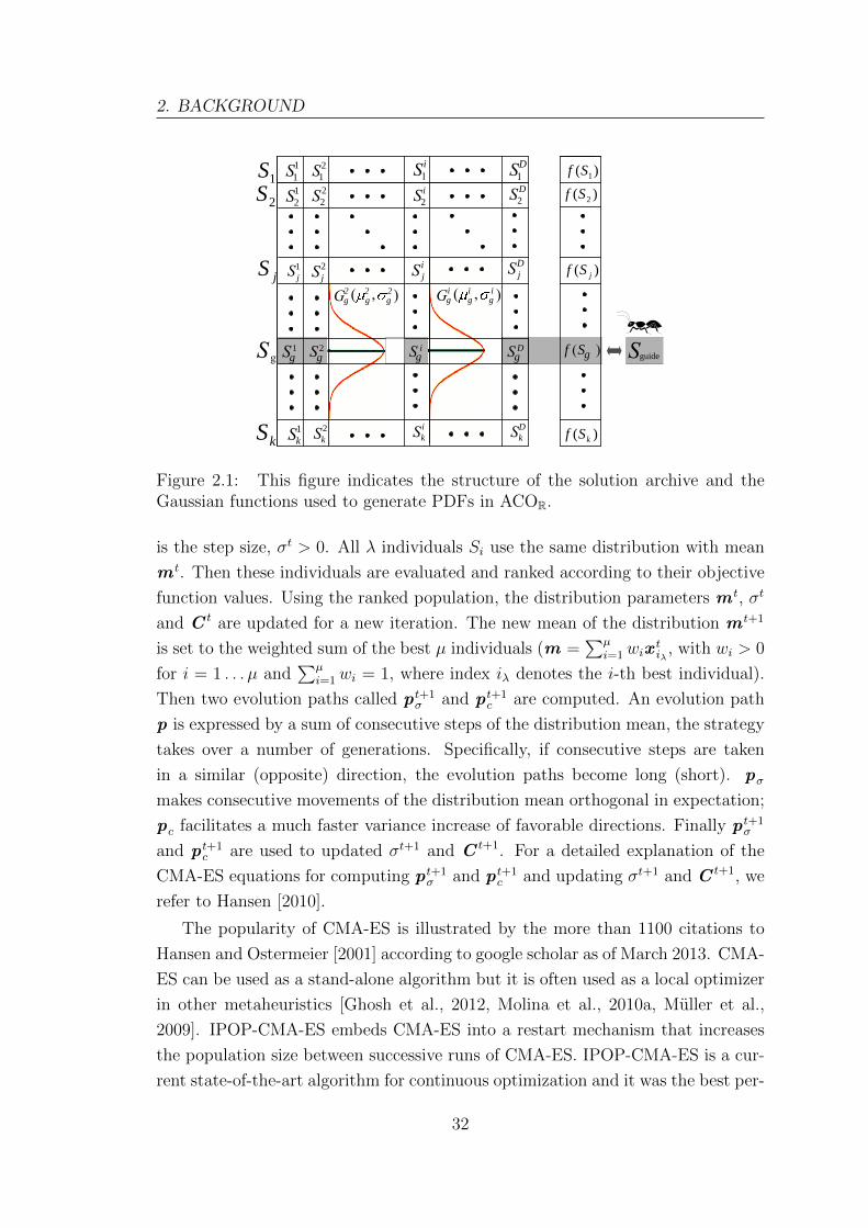
2. BACKGROUND
)( 1Sf
)( kSf
)( jSf
)( 2Sf1S2S
kS
jS
i11
2122
12
i2
ij
1j
2j
1k
2k
ik
D
D2
Dj
Dk
igg
igi
i21 D Sfgggg g
2gg
2g2
guide
Figure 2.1: This figure indicates the structure of the solution archive and theGaussian functions used to generate PDFs in ACOR.
is the step size, σt > 0. All λ individuals Si use the same distribution with mean
m t. Then these individuals are evaluated and ranked according to their objective
function values. Using the ranked population, the distribution parameters m t, σt
and C t are updated for a new iteration. The new mean of the distribution m t+1
is set to the weighted sum of the best µ individuals (m =∑µ
i=1wixtiλ
, with wi > 0
for i = 1 . . . µ and∑µ
i=1wi = 1, where index iλ denotes the i-th best individual).
Then two evolution paths called p t+1σ and p t+1
c are computed. An evolution path
p is expressed by a sum of consecutive steps of the distribution mean, the strategy
takes over a number of generations. Specifically, if consecutive steps are taken
in a similar (opposite) direction, the evolution paths become long (short). pσmakes consecutive movements of the distribution mean orthogonal in expectation;
pc facilitates a much faster variance increase of favorable directions. Finally p t+1σ
and p t+1c are used to updated σt+1 and C t+1. For a detailed explanation of the
CMA-ES equations for computing p t+1σ and p t+1
c and updating σt+1 and C t+1, we
refer to Hansen [2010].
The popularity of CMA-ES is illustrated by the more than 1100 citations to
Hansen and Ostermeier [2001] according to google scholar as of March 2013. CMA-
ES can be used as a stand-alone algorithm but it is often used as a local optimizer
in other metaheuristics [Ghosh et al., 2012, Molina et al., 2010a, Muller et al.,
2009]. IPOP-CMA-ES embeds CMA-ES into a restart mechanism that increases
the population size between successive runs of CMA-ES. IPOP-CMA-ES is a cur-
rent state-of-the-art algorithm for continuous optimization and it was the best per-
32
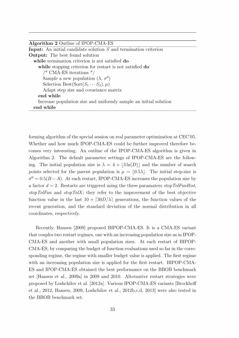
Algorithm 2 Outline of IPOP-CMA-ES
Input: An initial candidate solution S and termination criterionOutput: The best found solution
while termination criterion is not satisfied dowhile stopping criterion for restart is not satisfied do
/* CMA-ES iterations */Sample a new population (λ, σ0)Selection Best(Sort(S1 · · ·Sλ), µ)Adapt step size and covariance matrix
end whileIncrease population size and uniformly sample an initial solution
end while
forming algorithm of the special session on real parameter optimization at CEC’05.
Whether and how much IPOP-CMA-ES could be further improved therefore be-
comes very interesting. An outline of the IPOP-CMA-ES algorithm is given in
Algorithm 2. The default parameter settings of IPOP-CMA-ES are the follow-
ing. The initial population size is λ = 4 + b3 ln(D)c and the number of search
points selected for the parent population is µ = b0.5λc. The initial step-size is
σ0 = 0.5(B−A). At each restart, IPOP-CMA-ES increases the population size by
a factor d = 2. Restarts are triggered using the three paramaters stopTolFunHist,
stopTolFun and stopTolX ; they refer to the improvement of the best objective
function value in the last 10 + d30D/λe generations, the function values of the
recent generation, and the standard deviation of the normal distribution in all
coordinates, respectively.
Recently, Hansen [2009] proposed BIPOP-CMA-ES. It is a CMA-ES variant
that couples two restart regimes, one with an increasing population size as in IPOP-
CMA-ES and another with small population sizes. At each restart of BIPOP-
CMA-ES, by comparing the budget of function evaluations used so far in the corre-
sponding regime, the regime with smaller budget value is applied. The first regime
with an increasing population size is applied for the first restart. BIPOP-CMA-
ES and IPOP-CMA-ES obtained the best performance on the BBOB benchmark
set [Hansen et al., 2009a] in 2009 and 2010. Alternative restart strategies were
proposed by Loshchilov et al. [2012a]. Various IPOP-CMA-ES variants [Brockhoff
et al., 2012, Hansen, 2009, Loshchilov et al., 2012b,c,d, 2013] were also tested in
the BBOB benchmark set.
33

2. BACKGROUND
2.4 Automatic algorithm configuration
Assigning appropriate values for the parameters of optimization algorithms is an
important task [Birattari, 2009]. Although algorithm designers have spent a con-
siderable effort in the design choices and certainly also in the definition of its
parameters, over the last few years evidence has arisen that many algorithms’
performance can be improved by considering automatic algorithm configuration
and tuning tools [Adenso-Diaz and Laguna, 2006, Balaprakash et al., 2007, Bartz-
Beielstein, 2006, Birattari et al., 2002, Hutter et al., 2007, 2009a,b, Nannen and
Eiben, 2007]. Many successful studies involve tuning discrete optimization algo-
rithms [Balaprakash et al., 2007, Birattari et al., 2002, Hutter et al., 2009b] and
also continuous optimization algorithms [Hutter et al., 2009a, Montes de Oca et al.,
2011, Smit and Eiben, 2009, Yuan et al., 2010].
In the design of algorithm frameworks, the entries of algorithmic components
can be designed as tunable parameters. The combination of algorithmic compo-
nents via automatic algorithm configuration tools has also shown its extraordi-
nary potential for obtaining new state-of-the-art algorithms. For instance, Khud-
aBukhsh et al. [2009] proposed the SATenstein framework and instantiated a new
state-of-the-art local search algorithm for the SAT problem. Lopez-Ibanez and
Stutzle [2010], Lopez-Ibanez and Stutzle [2012] automatically configured a multi-
objective ACO algorithm that outperformed previously proposed multi-objective
ACO algorithms for the bi-objective traveling salesman problem. Dubois-Lacoste
et al. [2011] configured new state-of-the-art algorithms for five variants of multi-
objective flow-shop problems. More recently, the ideas behind the combination
of algorithm frameworks and automatic algorithm configuration techniques have
been extended to the programming by optimization paradigm [Hoos, 2012].
2.4.1 Iterated F-Race
In this thesis, we employ Iterated F-Race [Birattari et al., 2010], a racing algorithm
for algorithm configuration that is included in the irace package [Lopez-Ibanez
et al., 2011] for automatic algorithm configuration and parameter tuning. Iterated
F-Race is an algorithm that repeatedly applies F-Race [Birattari et al., 2002] to a
set of candidate configurations that are generated via a sampling mechanism that
intensifies the search around the best found configurations. The generated candi-
date configurations then perform a “race”. At each step of the race, each surviving
candidate configuration is run on one training problem. Poor performing candi-
34
date configurations are eliminated from the race based on the result of statistical
tests. To this aim, the results of each surviving configuration on the same training
problem is ranked. Note that this ranking corresponds to blocking in statistical
tests since ranks are determined on a same training problem. In fact, ranking is
useful in the context of continuous and mixed-variable function optimization to
account for the different ranges of the values of the benchmark functions. With-
out ranking, few functions with large values would dominate the evaluation of the
algorithm performance. Based on the obtained ranks, the Friedman two-way anal-
ysis of variance by ranks checks whether sufficient statistical evidence is gathered
that indicates that some configurations behave differently from the rest. If the
null hypothesis of the Friedman test is rejected, Friedman post-tests are used to
eliminate the statistically worse performing candidates. The irace automatic con-
figuration tool handles four parameter types: continuous (r), integer (i), ordinal
(o) and categorical (c).
With Iterated F-race, algorithm parameters are tuned using a machine learning
approach in which an algorithm is trained on a set of problem instances and later
tested on another set. In this thesis, the performance measure for tuning is the
error of the objective function value obtained by the tuned algorithm after a certain
number of function evaluations. The error value is defined as f(S)− f(S∗), where
S is a candidate solution and S∗ is an optimal solution. In [Lopez-Ibanez et al.,
2012], we used the hypervolume as performance measure for tuning, a well-known
quality measure in multi-objective optimization, to assign a single numerical value
to the anytime behavior of an algorithm’s run.
2.4.2 Tuning methodology
This thesis is not the first to try to further tune continuous optimization algo-
rithm using automatic algorithm configuration tools. A PSO algorithm was used
by Bartz-Beielstein [2006] as a benchmark algorithm to be tuned for evaluating
Sequential Parameter Optimization (SPO). CMA-ES was used by Hutter et al.
[2009a] as a benchmark algorithm to be tuned for evaluating SPO+, their im-
proved variant of SPO [Bartz-Beielstein, 2006]. Following earlier work on SPO,
they tuned CMA-ES only on individual functions, thus, in this sense “overtuning”
CMA-ES on individual functions. (One has to remark, however, that the inter-
est of Hutter et al. [2009a] was to evaluate SPO and the improved variant SPO+
rather than proposing a new, generally improved parameter setting for CMA-ES.)
Another attempt of tuning a variant of CMA-ES was made by Smit and Eiben
35

2. BACKGROUND
[2010]. From a tuning perspective, it should be mentioned that they tuned their
algorithm on multiple functions. For the tuning, they used the CMA-ES variant
they used on each ten dimensional function, then they were running the tests with
the tuned algorithm on the same functions of dimension ten. Same was done by
Montes de Oca et al. [2011] for re-designing and tuning a PSO algorithm for large
scale continuous function optimization.
In the methodological approach to tuning continuous optimization algorithms,
this thesis tries to avoid a bias of the results obtained due to potentially overtuning
[Birattari, 2009] the algorithm on the same benchmark functions as those on which
the algorithm is tested. As such, this gives a better assessment of the potential
for what concerns the tuning of continuous optimizers as we have a separation
between tuning and test set. In this thesis, the tuning and test sets involve three
degrees of separation as follows:
• A separation of dimensionality between tuning and test set. For instance,
we tuned algorithms on small dimensional functions and later tested them
on (much) larger dimensional versions of the same functions. [Liao et al.,
2011c, Montes de Oca et al., 2011].
• A separation of the functions used in the tuning and test set. For instance,
we tuned algorithms on small dimensional functions and later tested them
on a different set of functions. [Liao and Stutzle, 2013, Liao et al., 2013a,
Lopez-Ibanez et al., 2012].
• A separation between tuning functions and real world problems. For in-
stance, we tuned algorithms on artificial benchmark functions and later
tested them on real-word optimization problems. [Liao et al., 2013b]
The differences in the applied approaches to tuning with respect to the sepa-
ration of tuning and test sets is summarized in Figure 2.2.
2.5 Summary
In this chapter, we described the models of continuous optimization problems,
and reviewed the main optimization techniques (i.e., local search algorithms and
metaheuristic based algorithms) and discussed the main benchmark function sets
that are relevant for this thesis. We also described the models of mixed discrete-
continuous optimization problems, and classified the main approaches to tackle
mixed variable problems from the literature. We explained in some more detail
36

Figure 2.2: Summary of the methodological approach to tuning continuous opti-mization algorithms from few recent articles [Bartz-Beielstein, 2006, Hutter et al.,2009a, Smit and Eiben, 2010] and this thesis. The approaches differ in the usage ofa single versus multiple functions and the degree of separation between tuning andtest set. The difference of colors between tuning and test set indicates a separationof the functions used in the tuning and test set.
37

2. BACKGROUND
the two basic algorithms ACOR and CMA-ES, on which large parts of this thesis
rely on. We described an automatic algorithm configuration technique and the
tuning methodologies we used in the thesis.
38

Chapter 3
UACOR: A unified ACO algorithm for continuous opti-mization
Metaheuristics are a family of optimization techniques that have seen increasingly
rapid development and have been applied to numerous problems over the past
few years. A prominent metaheuristic is ant colony optimization (ACO). ACO
is inspired by the ants’ foraging behavior and it was first applied to solve dis-
crete optimization problems [Dorigo and Stutzle, 2004, Dorigo et al., 1991, 1996].
Recently, adaptations of ACO to continuous optimization problems were intro-
duced. Socha and Dorigo [2008] proposed one of the now most popular ACO
algorithms for continuous domains, called ACOR. It uses a solution archive as
a form of pheromone model for the derivation of a probability distribution over
the search space. Leguizamon and Coello [2010] proposed an extension of ACOR,
called DACOR, that had the goal of better maintaining diversity during the search.
Subsequently, we proposed IACOR-LS, an incremental ant colony algorithm with
local search for continuous optimization [Liao et al., 2011b]. IACOR-LS uses a
growing solution archive as an extra search diversification mechanism and a local
search to intensify the search.
In this chapter, we propose an ACO algorithm for continuous optimization,
which combines algorithmic components from ACOR, DACOR and IACOR-LS.
We call this algorithm UACOR. From UACOR, one can instantiate the original
ACOR, DACOR and IACOR-LS algorithms by using specific combinations of the
available algorithmic components and parameter settings. However, one also can
obtain combinations of the algorithmic components that are different from any
of the already proposed ones, that is, one may instantiate new, continuous ACO
algorithms. UACOR’s design makes the automatic generation of high performance
continuous ACO algorithms possible through the use of automatic algorithm con-
figuration tools.
39

3. UACOR: A UNIFIED ACO ALGORITHM FOR CONTINUOUSOPTIMIZATION
The combination of algorithmic components via automatic algorithm configu-
ration tools has already shown its high potential for obtaining new state-of-the-art
algorithms for combinatorial optimization problems. For example, Dubois-Lacoste
et al. [2011], KhudaBukhsh et al. [2009], Lopez-Ibanez and Stutzle [2012] config-
ured new state-of-the-art algorithms for the SAT problem, the bi-objective travel-
ing salesman problem and the multi-objective flow-shop problem, respectively.
UACOR is a highly configurable algorithm, and thus it can also be considered
a framework from which new state-of-the-art ACO algorithms for continuous op-
timization can be derived. In this chapter, we show how this can be done through
the use of an automatic configuration tool. In particular, we use Iterated F-race
[Birattari et al., 2010] as implemented in the irace package [Lopez-Ibanez et al.,
2011]. As the set of training benchmark functions we use low dimensional versions
of the functions used in the SOCO and CEC’05 benchmark sets. We configure
two new ACO variants; UACOR-s is configured on the SOCO benchmark (the -s
suffix stands for SOCO) set and UACOR-c on the CEC’05 benchmark set (the
-c suffix stands for CEC). UACOR-s and UACOR-c are then tested on higher di-
mensional versions of the SOCO and CEC’05 benchmark functions. The results
show that (i) UACOR-s performs superior or competitive to all the 16 algorithms
benchmarked on the SOCO function set and that (ii) UACOR-c performs compet-
itive to IPOP-CMA-ES [Auger and Hansen, 2005] and superior to other five recent
state-of-the-art algorithms benchmarked on the CEC’05 function set. These ex-
perimental results illustrate the high potential of ACO algorithms for continuous
optimization. To the best of our knowledge, this is also the first trial where a con-
tinuous optimizer framework is automatically configured. Previous applications of
automatic configuration for continuous optimization were applied to already fully
designed algorithms. Finally we re-design UACOR by implementing CMA-ES
[Hansen and Ostermeier, 1996, 2001, Hansen et al., 2003] as an alternative local
search procedure, which further improves the performance of UACOR.
The chapter is organized as follows. Section 3.1 introduces ACO for continuous
domains, reviews the three continuous ACO algorithms underlying UACOR, and
identifies their algorithmic components in a component-wise view. Section 3.2 de-
scribes UACOR. In Section 3.3, we automatically configure UACOR to instantiate
UACOR-s and UACOR-c and in Section 3.4, we evaluate their performance. The
performance of a re-designed and improved UACOR is shown in Section 3.5 and
conclude in Section 3.6.
40

3.1 ACO algorithms for continuous optimization
The UACOR framework build upon and extends the ACOR algorithm for continu-
ous optimization. In fact, from UACOR we can also instantiate directly the ACOR
algorithm. The main details of the ACOR algorithm have already been described
in Section 2.3.1 and we refer the reader to the details described there. Next we de-
scribe DACOR [Leguizamon and Coello, 2010] and IACOR-LS [Liao et al., 2011b],
two more recent ACO algorithms for continuous optimization.
DACOR
Different from ACOR, DACOR keeps the number of ants (Na) equal to the solution
archive size k and each of the Na ants constructs at each algorithm iteration a
new solution. A further difference of DACOR with respect to ACOR is the specific
choice rule for the guiding solution Sguide. With a probability Qbest ∈ [0, 1], ant j
chooses as Sguide the best solution, Sbest, in the archive; with a probability 1−Qbest,
it chooses as Sguide the solution Sj. A new solution is generated in the same way
as in ACOR, and then compared to Sj (independently of whether Sbest or Sj was
chosen as guiding solution). If the newly generated solution is better than Sj, it
replaces Sj in the archive; otherwise it is discarded. This replacement strategy is
different from the one used in ACOR in which all the solutions in the archive and
all the newly generated ones compete.
IACOR-LS
IACOR-LS’s main distinctive features are a solution archive whose size increases
over time to enhance the algorithm’s search diversification, and a local search
procedure to enhance its search intensification [Liao et al., 2011b]. Additionally,
IACOR-LS uses a different choice rule for the guiding solution than ACOR. At each
algorithm iteration of IACOR-LS, the best solution in the archive Sbest is chosen
as the guiding solution Sguide with a probability equal to the value of a parameter
EliteQbest ∈ [0, 1]; with a probability of 1−EliteQbest, each solution in the archive
is used as Sguide to generate a new solution. With this choice rule, either only one
new solution is constructed by an “elite” guiding solution or k new solutions are
constructed by k ants at each algorithm iteration. This latter aspect makes the
action choice roles of IACOR-LS also different from the one used in DACOR. Each
new solution is constructed in the same way as in ACOR. Finally, Sguide and the
newly generated solution are compared. If the newly generated solution is better
41

3. UACOR: A UNIFIED ACO ALGORITHM FOR CONTINUOUSOPTIMIZATION
than Sguide, it replaces it in the archive; otherwise it is discarded.
IACOR-LS initializes the archive with InitAS solutions. Every GrowthIter it-
erations a new solution is added to the archive until a maximum archive size is
reached. The new solution is initialized as follows:
Snew = Srand + rand(0, 1)(Sbest − Srand) , (3.1)
where Srand is a random solution and rand(0, 1) is a random number uniformly
distributed in [0, 1).
In IACOR-LS, the local search procedure is called at each iteration and for
LsIter iterations. If the local search succeeds in improving the solution from which
it is called, this improved solution replaces the original solution in the archive. The
maximum number of times the local search procedure is called from the same ini-
tial solution is limited to LsFailures calls. The initial solution for the local search
is chosen as follows. The best solution is deterministically chosen as the initial
solution if it has been called less than LsFailures times. Otherwise a random solu-
tion from the archive is chosen as the initial solution, excluding all those solutions
for which the number of times they have been chosen as initial solutions is equal
to LsFailures.
The step size to be used in the local search procedure is set as follows. First,
a solution different from the best one is chosen randomly in the archive. The step
size is then set to the maximum norm (|| · ||∞) of the vector that separates this
random solution from the best solution. As a result, step sizes tend to decrease
upon convergence of the algorithm and, in this sense, the step sizes are chosen
adaptively to focus the local search around the best-so-far solution. In our previous
experiments, Powell’s conjugate directions set [Powell, 1964] and Lin-Yu Tseng’s
Mtsls1 [Tseng and Chen, 2008] local search methods (see also Section 2.1.1) have
shown very good performance.
IACOR-LS uses a default restart mechanism that restarts the algorithm and
re-initializes the archive of size InitAS with the best-so-far solution Sbest and Ini-
tAS−1 random solutions. The restart criterion is the number of consecutive it-
erations, StagIter, with a relative solution improvement lower than a threshold ε.
IACOR-LS also integrates a second restart mechanism, which consists in restarting
and initializing a new initial archive of size RestartAS (RestartAS is a parameter
different from InitAS ) with Sbest in the current archive and RestartAS−1 solutions
that are initialized at positions biased around Sbest; these positions are defined by
Sbest +10Shakefactor · (Sbest − Srand). The restart criterion is the number of consec-
42

utive iterations, StagIter, with a relative solution improvement percentage lower
than a certain threshold 10StagThresh.
3.1.1 Algorithmic components
We define several algorithmic components for UACOR by abstracting the partic-
ular design alternatives taken in ACOR, DACOR and IACOR-LS. This results in
seven main groups of algorithmic components, which are described next, before
detailing the outline of UACOR.
1. Mode. Two alternative UACOR modes, called DefaultMode and EliteMode,
are identified. DefaultMode consists in deploying a number of ants in each
algorithm iteration to construct solutions. EliteMode allows in each algo-
rithm iteration to deploy only one “elite” ant with a probability of EliteQbest
∈ [0, 1]. The “elite” ant selects Sbest in the archive as Sguide to construct a
new solution.
2. Number of ants. Two design choices for defining the number of ants
deployed are identified. Na defines the number of ants as an independent
parameter (Na ≤ k) while NaIsAS defines the number of ants to be equal to
k, the size of the solution archive.
3. Choice of guiding solution. This algorithmic component chooses how to
select Sguide to sample new solutions. Three design choices are identified:
(i) Sbest is selected as Sguide with a probability Qbest ∈ [0, 1]; (ii) Sguide is
probabilistically selected from the solutions in the archive depending on their
weight; (iii) solution Sl is selected as Sguide, where l is the index of the
currently deployed ant.
4. Update of solution archive. The update of the solution archive con-
cerns the replacement of solutions in the archive. We identified three design
choices. A parameter RmLocalWorse defines whether UACOR globally re-
moves the Na worst solutions among all k+Na solutions, or whether UACOR
makes the decision about the acceptance of Sl locally. In the latter case, we
use a parameter SnewvsGsol to decide whether the solution generated by ant
l is compared with Sguide or with the previous l-th solution to remove the
worse one.
5. Local search. We consider three options for the use of a local search pro-
cedure. If parameter LsType is set to F (for false), no local search procedure
43

3. UACOR: A UNIFIED ACO ALGORITHM FOR CONTINUOUSOPTIMIZATION
is used. Otherwise, LsType invokes either Powell’s conjugate directions set
[Powell, 1964] or Mtsls1 [Tseng and Chen, 2008]. Both local search proce-
dures use a dynamic calling strategy and an adaptive step size, which follow
the choices taken for IACOR-LS.
6. Incremental archive size. The possibility of incrementing the archive size
is considered. If parameter IsIncrement is set to F, the incremental archive
mechanism is not used. Otherwise, if IsIncrement is set to T (for true),
UACOR invokes the incremental archive mechanism.
7. Restart mechanism. Three options for the restart mechanism are identi-
fied. If parameter RestartType is set to F, the restart mechanism is not used.
Otherwise, RestartType invokes either of the two restart mechanisms, which
are introduced in IACOR-LS. They are labeled as 1st and 2nd, respectively.
Table 3.1 summarizes the algorithmic components defined above and their op-
tions. Some algorithmic components are only significant for a specific value of other
components. We discuss the connection between these algorithmic components in
Section 3.2.
44
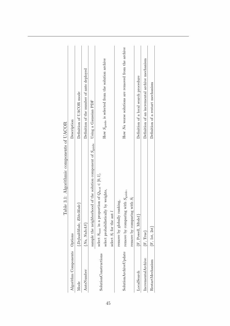
Tab
le3.
1:A
lgor
ithm
icco
mp
onen
tsof
UA
CO
R
Alg
orit
hm
Com
pon
ents
Op
tion
sD
escr
ipti
on
Mod
eD
efaultMode,
EliteMode
Defi
nit
ion
of
UA
CO
Rm
od
e
Ants
Nu
mb
erN
a,NaIsAS
Defi
nit
ion
of
the
nu
mb
erof
ants
dep
loyed
Sol
uti
onC
onst
ruct
ion
s
sam
ple
the
nei
ghb
orh
ood
ofth
eso
luti
on
com
pon
ent
ofSguide
Usi
ng
aG
au
ssia
nP
DF
sele
ctSbest
ina
pro
por
tion
ofQbest∈
[0,1
],
How
Sguide
isse
lect
edfr
om
the
solu
tion
arc
hiv
ese
lect
pro
bab
ilis
tica
lly
by
wei
ghts
,
sele
ctSl
for
the
antl
Sol
uti
onA
rch
iveU
pd
ate
rem
ove
by
glob
ally
ran
kin
g,
How
Na
wors
eso
luti
on
sare
rem
oved
from
the
arc
hiv
ere
mov
eby
com
par
ing
wit
hSguide,
rem
ove
by
com
par
ing
wit
hSl
Loca
lSea
rch
F,
Pow
ell,
Mts
ls1
Defi
nit
ion
of
alo
cal
searc
hp
roce
du
re
Incr
emen
talA
rch
ive
F,
Tru
eD
efin
itio
nof
an
incr
emen
tal
arc
hiv
em
ech
an
ism
Res
tart
Mec
han
ism
F,
1st,
2st
Defi
nit
ion
of
are
start
mec
hanis
m
45

3. UACOR: A UNIFIED ACO ALGORITHM FOR CONTINUOUSOPTIMIZATION
3.2 UACOR
The three ACO algorithms described in the previous section as well as many others
that may result from the combination of their components are subsumed under the
general algorithmic structure provided by UACOR. In this section, we describe the
connections of the algorithmic components of UACOR by a flowchart and show
how from UACOR we can instantiate the algorithms ACOR, DACOR and IACOR-
LS. The flowchart of UACOR is given in Fig. 3.1. The related parameters are
given in Table 3.2. Some settings take effect in the context of certain values of
other settings.
UACOR starts by randomly initializing and evaluating the solution archive of
size InitAS. Next, UACOR selects a mode, which can be either the default mode
or an elite mode.
We first describe the default mode, which is invoked if parameter DefaultMode
is set to T (true). At each iteration, Na new solutions are probabilistically con-
structed by Na ants (recall that an ant in our case is the process through which a
solution is generated). If the parameter NaIsAS is set to T, the number of ants is
kept equal to the size of the solution archive. If the parameter NaIsAS is set to
F (false), a parameter Na, Na ≤ k, is activated. Each ant uses a choice rule for
the guiding solution. The parameter Qbest ∈ [0, 1] controls the probability of using
Sbest as Sguide. With a probability 1−Qbest, Sguide is selected in one of two different
ways. If parameter WeightGsol is T, Sguide is probabilistically selected from the
solutions in the archive by their weights as defined by Equation 2.1. Otherwise,
solution Sl (l is associated with the index of the current ant to be deployed) is
chosen as Sguide. Once Sguide is selected, a new solution is generated. This process
is repeated for each of the Na ants. Next, UACOR updates the solution archive
by removing Na solutions. If parameter RmLocalWorse is F, UACOR removes
the Na worst solutions among all the k + Na solutions as in ACOR. If parameter
RmLocalWorse is T, one of two possibilities is considered. If parameter SnewvsG-
sol is T, each newly generated solution is compared to the corresponding Sguide to
remove the worse one; otherwise, it is compared to the corresponding Sl to remove
the worse one. Finally, a new solution archive is generated.
The elite mode is invoked if parameter DefaultMode is set to F. The elite
mode at each algorithm iteration deploys only one “elite” ant. With a probability
EliteQbest, 0 ≤ EliteQbest ≤ 1, it selects Sbest in the archive as Sguide. If the newly
generated solution is better than this Sbest, it replaces it in the solution archive;
with a probability 1−EliteQbest the solution construction follows the default mode.
46

b
Qbest >rand
WeightGsol
Set a guiding solution
Sample Gaussian around the guiding solution
Initialize and evaluate solution archive
T
RmLocalWorse
T
SnewvsGsol
DefaultModeF
EliteQbest >rand T
End
T
F
Select Sbest
Sample Gaussian
Generate a new solution
Remove a worse solutoin
Select Sbest
T
While termination criterion not satisfied
For ( l = 1 to Na )
NaIsAS
T
Generate a new solution
T
F
Local search
Incremental archive mechnism
Restart mechanism
Snew vs. Sbest
Begin
Set a guiding solution
Na <= k
FF
F
Remove Na worse solutions
F
Sort Na+AS solutions Snew vs. lS
Select lS
Generate a new solution archive
Na = k
Select Mode
Set number of ants
Na k Set Na <= kT
Select S by weight
F
Snew vs. Gsol
Optional
Figure 3.1: A flowchart for UACOR. For an explanation of the parameters werefer to the text.
47

3. UACOR: A UNIFIED ACO ALGORITHM FOR CONTINUOUSOPTIMIZATION
After updating the solution archive, UACOR sequentially considers three pro-
cedures. These are a local search procedure, a mechanism for increasing the archive
size and a restart mechanism, respectively. Recall that the options of these proce-
dures were described in Section 3.1.
We use a simple penalty mechanism to handle bound constraints for UACOR.
We use
P (x) = fes ·D∑i=1
Bound(xi) , (3.2)
where Bound(xi) is defined as
Bound(xi) =
0, if xmin ≤ xi ≤ xmax
(xmin − xi)2, if xi < xmin
(xmax − xi)2, if xi > xmax
(3.3)
and xmin and xmax are the minimum and maximum limits of the search range,
respectively, and fes is the number of function evaluations that have been used
so far. For avoiding that the final solution is outside the bounds, the bound
constraints are enforced by clamping the final solution S to the nearest solution
on the bounds, resulting in solution S ′, if S violates some bound constraints. If
S ′ is worse than the best feasible solution found in the optimization process, S ′ is
replaced by it.
3.3 Automatic algorithm configuration
We automatically configure UACOR before evaluating its performance on bench-
mark functions. As the benchmark functions, we employ the 19 functions from
the SOCO benchmark set [Herrera et al., 2010] (fsoco1-fsoco19) and the 25 functions
from the CEC05 benchmark set [Suganthan et al., 2005] (fcec1-fcec25). Note that
in both benchmark sets, the functions allow for different dimensionalities. These
two benchmark sets have been chosen as they have become standard benchmark
sets for testing continuous optimizers. The SOCO benchmark set was used in a
special issue of the journal Soft Computing and it extends the benchmark sets
of earlier benchmarking studies on the scaling behavior of continuous optimizers
such as the one held at the CEC’08 conference. The CEC’05 benchmark set was
used for a comparison of evolutionary optimizers at the special session on real pa-
rameter optimization of CEC’05 conference [Suganthan et al., 2005]. Classified by
48

function characteristics, the SOCO benchmark set consists of seven unimodal and
12 multimodal functions, or, four separable and 15 non-separable functions. The
CEC’05 benchmark set consists of five unimodal and 20 multimodal functions, or,
two separable and 23 non-separable functions. For a detailed description of the
benchmark functions, we refer the reader to [Herrera et al., 2010, Suganthan et al.,
2005], and to the description in Section 2.1.3.
In our experiments, we follow the termination conditions suggested for the
SOCO and CEC benchmarks [Herrera et al., 2010, Suganthan et al., 2005] to make
our results comparable to those of other papers. In particular, we use a maximum
of 5 000×D function evaluations for the SOCO functions, and 10 000×D for the
CEC’05 functions, where D is the dimensionality of a function.
For automatically configuring UACOR, we employ Iterated F-Race [Birattari
et al., 2010], a method for automatic algorithm configuration that is included in
the irace package [Lopez-Ibanez et al., 2011] and that was described in Section
2.4.1. In a nutshell, Iterated F-Race repeatedly applies F-Race to a set of candi-
date configurations. F-Race is a racing method that at each iteration applies all
surviving candidate configurations to an instance of a combinatorial problem or a
function in the continuous optimization case. If a candidate configuration is found
to perform statistically worse than others (as determined by the Friedman two-way
analysis of variance by ranks and its associated post-tests), it is eliminated from
the race. F-race finishes when only one candidate survive or the allocated com-
putation budget to the race is used. Iterated F-Race then samples new candidate
configurations around the best candidate configurations found so far. The whole
process is repeated for a number of iterations (hence the name Iterated F-Race).
The automatic configuration tool handles all parameter types of UACOR: con-
tinuous (r), integer (i) and categorical (c). The performance measure used for
tuning is the error of the objective function value obtained by the tuned algo-
rithm after a certain number of function evaluations. The error value is defined
as f(S) − f(S∗), where S is a candidate solution and S∗ is the optimal solution.
In the automatic tuning process, the maximum budget is set to 5 000 runs of UA-
COR. The settings of Iterated F-Race that we used in our experiments are the
default [Birattari et al., 2010, Lopez-Ibanez et al., 2011]. We conduct automatic
configuration for UACOR in two stages. In the first stage, we tuned UACOR on
the SOCO training instances to instantiate UACOR-s. 19 SOCO benchmark func-
tions of dimension 10 were sampled as training instances in a random order. In
the second stage, we tuned UACOR on the CEC’05 training instances to instanti-
ate UACOR-c. 25 CEC’05 benchmark functions of dimension 10 were sampled as
49

3. UACOR: A UNIFIED ACO ALGORITHM FOR CONTINUOUSOPTIMIZATION
training instances in a random order.
The tuned parameter settings for both, UACOR-s and UACOR-c, are pre-
sented in the central and right part of Table 3.2. This table also gives the parame-
ter settings for the UACOR’s instantiations of ACOR, DACOR and IACOR-Mtsls1.
Their parameters were also automatically tuned as mentioned above for the SOCO
and CEC’05 benchmark sets, respectively, and for these specific parameter con-
figurations we again use the extensions ’-s’ and ’-c’ depending on the benchmark
functions used for automatic configuration. Considering that UACOR-s does not
use the restart mechanisms of UACOR after tuning and UACOR-c does, when
tuning these three ACO algorithms on the SOCO training instances, we deploy
them as proposed in the original literature; when tuning them on CEC’05 training
instances, we extend them to use the restart mechanisms of UACOR to improve
performance.
As a further illustration of the respective algorithm structures, we highlight
UACOR-s and UACOR-c in the flowcharts of UACOR in Fig. 3.2 and 3.3. Both
use DefaultMode, select Sbest as Sguide with a probability Qbest ∈ [0, 1], use Mtsls1
local search and the incremental archive mechanism. The parameter settings in
which they differ, imply a more explorative search behavior of UACOR-c than
that of UACOR-s. In fact, (i) UACOR-c sets the number of ants equal to the size
of the solution archive while UACOR-s defines it as an independent parameter
(Na ≤ k); (ii) UACOR-c frequently chooses all solutions of the archive as Sguide (as
in DACOR), while UACOR-s probabilistically selects Sguide based on its weight;
(iii) UACOR-c makes a local acceptance decision comparing Sl to Sguide, while
UACOR-s globally removes the Na worst solutions among all k+Na solutions; (iv)
UACOR-c uses a restart mechanism for diversifying the search while UACOR-s
does not. Considering parameter values, UACOR-c has larger initial archive size
and less iterations of local search exploitation, which is consistent with the idea of a
strong search exploration than UACOR-s; the larger values of Qbest and GrowthIter
would imply UACOR-c and UACOR-s differ. Similar remarks hold also for the
settings of the ’-c’ and ’-s’ variants of ACOR, DACOR and IACOR-Mtsls1. Note
that the more explorative settings on the CEC’05 benchmark set are somehow
in accordance with the perceived higher difficulty of this benchmark set than the
SOCO set. In fact, in the CEC’05 benchmark set the best available algorithms fail
to find quasi-optimal solutions much more frequently than in the SOCO benchmark
function set.
50

.T
able
3.2:
Th
ele
ftp
art
ofth
eta
ble
give
sth
eli
stof
par
amet
erse
ttin
gsan
dth
eir
dom
ain
s.S
ome
sett
ings
are
only
sign
ifica
nt
for
cert
ain
valu
esof
oth
erse
ttin
gs.
Th
ep
aram
eter
sett
ings
ofth
eau
tom
atic
ally
con
figu
red
algo
rith
ms
are
give
nin
the
centr
alp
art
and
the
righ
tp
art,
dep
end
ing
onw
hic
htr
ain
ing
set
ofb
ench
mar
kfu
nct
ion
sw
asu
sed
for
tun
ing.
Module
Par
aN
ame
Typ
eD
omai
nT
unin
gon
SO
CO
Tunin
gon
CE
C’0
5
AC
OR-s
DA
CO
R-s
IAC
OR-M
tsls
1-s
UA
CO
R-s
AC
OR-c
DA
CO
R-c
IAC
OR-M
tsls
1-c
UA
CO
R-c
Mode
DefaultMode
cT
,F
TT
FT
TT
FT
EliteQbest
r[0
,1]
**
0.0
508
**
*0.7
974
*
Def
Nan
ts
InitAS
i[2
0,10
0]87
40
648
92
81
54
66
NaIsAS
cT
,F
FT
TF
FT
TT
Na
i[2
,20
]2
**
16
14
**
*
Sol
Con
str
Qbest
r[0
,1]
00.1
193
00.1
895
00.1
287
00.5
351
WeightG
sol
cT
,F
TF
FT
TF
FF
qr
(0,
1)0.2
869
**
0.2
591
0.0
9401
**
*
ξr
(0,
1)0.7
187
0.6
705
0.8
782
0.6
511
0.6
998
0.7
357
0.9
164
0.6
945
SA
Up
dat
eRmLocalW
orse
cT
,F
FT
TF
FT
TT
Snew
vsGsol
cT
,F
*F
T*
*F
TT
LS
LsT
ype
cF,P
owel
l,M
tsls
1
FF
Mts
ls1
Mts
ls1
FF
Mts
ls1
Mts
ls1
LsIter
i[1
,10
0]*
*85
84
**
39
28
LsFailures
i[1
,20
]*
*1
8*
*3
7
IncA
rch
IsIncrem
ent
cT
,F
FF
TT
FF
TT
GrowthIter
i[1
,30
]*
*4
4*
*10
13
Res
tart
Mec
h
RestartType
cF,1
st,2
nd
FF
1st
F2n
d2n
d2n
d2n
d
StagIter
r[1
,10
00]
**
18
*939
313
611
StagT
hresh
r[-
15,
0]*
**
*-3
.386
-2.3
02
-3.0
41
-2.5
39
Shakefactor
r[-
15,
0]*
**
*-4
.993
-4.1
63
-0.0
4979
-0.0
2061
RestartAS
i[2
,10
0]*
**
*66
71
310
*den
otes
the
valu
eof
the
par
amet
eris
not
rele
vant
for
the
corr
esp
ondin
galg
ori
thm
.
51

3. UACOR: A UNIFIED ACO ALGORITHM FOR CONTINUOUSOPTIMIZATION
b
Qbest >rand
WeightGsol
Set a guiding solution
Sample Gaussian around the guiding solution
Initialize and evaluate solution archive
T
RmLocalWorse
DefaultMode
T
End
Select Sbest
T
While termination criterion not satisfied
For ( l = 1 to Na )
NaIsAS
Generate a new solution
F
Local search
Incremental archive mechnism
Begin
Na <= k
F
Remove Na worse solutions
Sort Na+AS solutions
Generate a new solution archive
Select Mode
Set number of ants
Set Na <= kT
Select S by weight
F
Mtsls1
UACOR-s
T
Figure 3.2: UACOR-s is highlighted in the flowchart of UACOR.
52

b
Qbest >rand
WeightGsol
Set a guiding solution
Sample Gaussian around the guiding solution
Initialize and evaluate solution archive
RmLocalWorse
T
SnewvsGsol
DefaultMode
T
End
Select Sbest
T
While termination criterion not satisfied
For ( l = 1 to Na )
NaIsAS
T
Generate a new solution
T
F
Local search
Incremental archive mechnism
Restart mechanism
Begin
F
Remove Na worse solutions
F
Select lS
Generate a new solution archive
Select Mode
Set number of ants
Na k
F
Snew vs. Gsol
Mtsls1
UACOR-c
2nd
T
Figure 3.3: UACOR-c is highlighted in the flowchart of UACOR.
53

3. UACOR: A UNIFIED ACO ALGORITHM FOR CONTINUOUSOPTIMIZATION
3.4 Algorithm evaluation
In this section, we evaluate UACOR-s and UACOR-c on the 19 SOCO benchmark
functions of dimension 100 and 25 CEC’05 benchmark functions of dimensions
30 and 50. Each algorithm was independently run 25 times on each function.
Whenever a run obtains a new best error value, we record the number of function
evaluations used, and the new best error value. Following the rules of the SOCO
algorithm comparison, error values lower than 10−14 are approximated to 10−14
(10−14 is referred as optimum threshold for SOCO functions). For CEC’05 func-
tions, error values lower than 10−8 are approximated to 10−8 (10−8 is the optimum
threshold for CEC’05 functions). On each benchmark function of each dimension-
ality we compute the average error obtained by an algorithm. These average errors
on all test functions in each benchmark set (SOCO or CEC’05) are then used to
compare the algorithms’ performance. To analyze the results we first use a Fried-
man test at the 0.05 α-level to determine whether there are significant differences
among the algorithms compared [Conover, 1998]. In fact, in all cases the null hy-
pothesis of equal performance is rejected and we then determine the significance of
the difference between the algorithms of interest based on the computed minimum
difference between the sum of the ranks that is statistically significant.
Experiments on SOCO benchmark set
First, we compare UACOR-s with the three ACO algorithms, ACOR-s, DACOR-s
and IACOR-Mtsls1-s. The left plot of Figure 3.4 shows that UACOR-s improves
upon these ACO algorithms on the distribution of average errors across the 19
SOCO benchmark functions. In particular, UACOR-s performs statistically sig-
nificantly better than ACOR-s and DACOR-s. This test is based on the average
error values that are reported in Table 3.3. In fact, on 14 of the 19 functions the
average error obtained by UACOR-s is below the optimum threshold, while for
ACOR-s, DACOR-s and IACOR-Mtsls1-s such low average error values are only
obtained 0, 1, and 8 times, respectively. (The main responsible for the large
differences between the performance of ACOR-s and DACOR-s on one side and
UACOR-s and IACOR-Mtsls1-s on the other side is due to the usage or not of
a local search procedure to improve candidate solutions.) The larger number of
optimum thresholds reached also is the reason why UACOR-s has a lower 75th per-
centile than ACOR-Mtsls1-s. Only on three functions, on which UACOR-s does
not reach the optimum threshold, it obtains slightly worse average errors than
IACOR-Mtsls1-s.
54

AC
Or−
s
DA
CO
r−s
IAC
Or−
mts
ls1
−s
UACOR−s
1e−14
1e−09
1e−04
1e+01
1e+06
+ +Optima 0 1 8 14
Ave
rage
Err
ors
of
Fitn
ess V
alu
e
Arc
hS
ize
=1
Arc
hS
ize=
50
Arc
hS
ize=
10
0
ArchSize=inc
1e−14
1e−09
1e−04
1e+01
1e+06
+Optima 6 8 9 14
Ave
rage
Err
ors
of
Fitn
ess V
alu
e
Figure 3.4: The box-plots show the distribution of the average errors obtainedon the 19 SOCO benchmark functions of dimension 100. The left plot comparesthe performance of UACOR-s with ACOR-s, DACOR-s and IACOR-Mtsls1-s. Theright plot shows the benefit of the incremental archive size used in UACOR-s. A+ symbol on top of each box-plot denotes a statistically significant difference atthe 0.05 α-level between the results obtained by the indicated algorithm and thoseobtained with UACOR-s. The absence of a symbol means that the difference is notstatistically significant. The numbers on top of a box-plot denote the number of theaverages below the optimum threshold 10−14 found by the indicated algorithms.
As a next step, we investigate the benefit of the incremental archive mechanism
used by UACOR-s when compared to a fixed archive size. The right boxplot of
Figure 3.4 shows that UACOR-s performs more effective than with archive sizes
fixed to 1, 50 and 100, respectively. (Note that for an archive size one, the resulting
algorithm is actually an iterated Mtsls1 local search algorithm [Tseng and Chen,
2008].) The differences are statistically significant for the archive sizes 1 and
the average errors of UACOR-s obtain the largest number of times the optimum
threshold number (14 versus 6, 8 and 9, respectively).
Finally, we compare UACOR-s with all 13 candidate algorithms published in
the SOCO special issue and to the three algorithms that were chosen as reference
algorithms.1 Figure 3.5 shows that UACOR-s performs statistically significantly
better than 10 other algorithms. Recall that IPOP-CMA-ES [Auger and Hansen,
1Information about these 16 algorithms is available athttp://sci2s.ugr.es/eamhco/CFP.php
55

3. UACOR: A UNIFIED ACO ALGORITHM FOR CONTINUOUSOPTIMIZATION
DE
CH
C
IPO
P−
CM
A−
ES
SO
UP
DE
DE
−D
40
−M
m
GO
DE
Ga
DE
jDE
lsco
p
Sa
DE
−M
MT
S
MO
S−
DE
MA
−S
SW
RP
SO
−vm
IPS
O−
Pow
ell
Evo
PR
Op
t
EM
32
3
VX
QR
1
UACOR−s
1e−14
1e−09
1e−04
1e+01
1e+06
+ + + + + + + + + +Optima 6 0 2 8 9 6 9 10 12 13 8 4 5 0 4 5 14
Ave
rag
e E
rro
rs o
f F
itn
ess V
alu
e
16 algorithms in SOCO
Figure 3.5: The box-plots show the distribution of the average errors obtained onthe 19 SOCO benchmark functions of dimension 100. The results obtained by thethree reference algorithms (left), 13 algorithms (middle) published in SOCO andUACOR-s (right) are shown on the left plot. The line at the bottom of the boxplotrepresents the optimum threshold (10−14). A + symbol on top of the two box-plot denotes a statistically significant difference at the 0.05 α-level between theresults obtained with the indicated algorithm and those obtained with UACOR-sdetected with a Friedman test and its associated post test on the 17 algorithms.The absence of a symbol means that the difference is not significant. The numberson top of a box-plot denote the number of averages below the optimum threshold10−14 found by the indicated algorithms.
2005] is considered to be a representative of the state-of-the-art for continuous
optimization and MA-SSW [Molina et al., 2010b, 2011] was the best performing
algorithm at the CEC’2010 competition on high-dimensional numerical optimiza-
tion. UACOR-s performs statistically significantly better than these two algo-
rithms. The best performing algorithm from the SOCO competition is MOS-DE
[LaTorre et al., 2011], an algorithm that combines differential evolution and the
Mtsls1 local search algorithm. It is noteworthy that UACOR-s performs compet-
itive to MOS-DE. Although UACOR-s does not obtain on more functions lower
average errors than MOS-DE than vice versa, UACOR-s gives on more functions
the zero threshold (14 versus 13).
56

Experiments on the CEC’05 benchmark set
We next evaluate UACOR-c on the CEC’05 benchmark set of dimension 30 and 50.
Tables 3.4 and 3.5 show the average error values across the 25 CEC’05 benchmark
functions obtained by UACOR-c, ACOR-c, DACOR-c, IACOR-Mtsls1-c, IPOP-
CMA-ES [Auger and Hansen, 2005] and other five recent state-of-the-art algo-
rithms.
Table 3.4 shows that UACOR-c gives across the 30 and 50 dimensional prob-
lems, on more functions lower average errors than ACOR-c, DACOR-c and IACOR-
Mtsls1-c than vice versa. Considering the average error values across all these
CEC’05 benchmark functions, UACOR-c performs statistically significantly better
than DACOR-c and IACOR-Mtsls1-c. It is important to highlight the following two
observations. First, UACOR-c significantly outperforms IACOR-Mtsls1-c on the
CEC’05 benchmarks while UACOR-s was superior to IACOR-Mtsls1-s but with-
out statistical significance. Second, the opposite happens with ACOR: ACOR-c
performs roughly on par with UACOR-c but ACOR-s is significantly outperformed
by UACOR-s on the SOCO benchmark set. (Recall that also ACOR and IACOR-
Mtsls1 were tuned for each of the benchmark sets.) In fact, the flexibility of UA-
COR makes it adaptable to each of the benchmark sets and allows it to outperform
other available ACO algorithms.
Of particular interest is the comparison between UACOR-c and IPOP-CMA-
ES, the data of which are taken from the literature [Auger and Hansen, 2005]. The
latter is an acknowledged state-of-the-art algorithm on the CEC’05 benchmark
set. UACOR-c shows competitive performance to IPOP-CMA-ES and it gives on
slightly more functions lower average errors than IPOP-CMA-ES than vice versa.
The average error values that correspond to a better result between UACOR-c and
IPOP-CMA-ES are highlighted in Table 3.4.
As a final step, we compare UACOR-c with five recent state-of-the-art contin-
uous optimization algorithms published since 2011. These reference algorithms in-
clude HDDE [Dorronsoro and Bouvry, 2011], Pro-JADE [Epitropakis et al., 2011],
Pro-SaDE [Epitropakis et al., 2011], Pro-DEGL [Epitropakis et al., 2011] and
ABC-MR [Akay and Karaboga, 2012]. In the original literature, these algorithms
were tested on the CEC’05 benchmark set for which the parameter values of the
algorithms were either set by experience or they were manually tuned. We di-
rectly obtain the data of the five algorithms on the CEC’05 benchmark set from
the original papers. Table 3.5 shows that UACOR-c gives on the 30 and 50 di-
mensional problems on more functions lower average errors than each of these five
57

3. UACOR: A UNIFIED ACO ALGORITHM FOR CONTINUOUSOPTIMIZATION
state-of-the-art algorithms. For each algorithm, Table 3.6 summarizes the average
ranking, the number of times the optimum thresholds is reached and the number
of lowest average error values obtained across all six algorithms that are compared.
Although with the exception of ABC-MR the differences to these algorithms are
not found to be statistically significant (neither are the differences among these al-
gorithms statistically significant), it is a noteworthy result that UACOR-c obtains
the best average ranking, the highest number of optimum thresholds and that it
is the best performing algorithm for most functions.
Table 3.3: The average errors obtained by ACOR-s, DACOR-s, IACOR-Mtsls1-s,MOS-DE and UACOR-s for each SOCO function. The numbers in parenthesis atthe bottom of the table represent the number of times an algorithm is better, equal orworse, respectively, than UACOR-s. Error values lower than 10−14 are approximatedto 10−14. The average errors that correspond to a better result between MOS-DEand UACOR-c are highlighted.
Dim fsoco ACOR-s DACOR-s IACOR-Mtsls1-s MOS-DE UACOR-s
100
fsoco1 5.32E−14 1.00E−14 1.00E−14 1.00E−14 1.00E−14fsoco2 2.77E+01 3.82E+01 5.27E−12 2.94E−12 6.53E−12fsoco3 1.96E+02 2.86E+03 4.77E+02 2.03E+01 3.81E+02fsoco4 6.34E+02 3.89E+02 1.00E−14 1.00E−14 1.00E−14fsoco5 2.96E−04 4.96E−01 1.00E−14 1.00E−14 1.00E−14fsoco6 2.04E−08 3.49E+00 1.00E−14 1.00E−14 1.00E−14fsoco7 9.94E−10 5.01E−01 1.00E−14 1.00E−14 1.00E−14fsoco8 4.39E+04 2.28E+04 1.39E+00 9.17E−02 1.54E+00fsoco9 4.78E+00 1.84E+02 1.62E−01 1.00E−14 1.00E−14fsoco10 2.75E+00 2.09E+01 1.00E−14 1.00E−14 1.00E−14fsoco11 3.96E+00 1.90E+02 1.67E−01 1.00E−14 1.00E−14fsoco12 1.13E+01 2.39E+02 4.01E−02 1.00E−14 1.00E−14fsoco13 1.47E+02 3.92E+02 4.19E+01 1.75E+01 9.31E+01fsoco14 3.40E+02 2.40E+02 9.23E+00 1.68E−11 1.00E−14fsoco15 5.89E−01 4.41E+00 1.00E−14 1.00E−14 1.00E−14fsoco16 1.61E+00 4.18E+02 4.24E−01 1.00E−14 1.00E−14fsoco17 6.27E+01 6.65E+02 8.40E+01 1.43E+01 5.30E+01fsoco18 1.57E+01 1.17E+02 1.07E−01 1.00E−14 1.00E−14fsoco19 1.48E+00 1.61E+01 1.00E−14 1.00E−14 1.00E−14
By fsoco (1, 0, 18)† (0, 1, 18)† (3, 8, 8) (5, 13, 1)
† denotes a significant difference between the corresponding algorithm and UACOR-s by a Fried-man test at the 0,05 α-level over the distribution of average errors of ACOR-s, DACOR-s,IACOR-Mtsls1-s and UACOR-s.
58

Table 3.4: The average errors obtained by ACOR-c, DACOR-c, IACOR-Mtsls1-c, IPOP-CMA-ES and UACOR-c for each CEC’05 function. The numbers in parenthesis at thebottom of the table represent the number of times an algorithm is better, equal or worse,respectively, compared to UACOR-c. Error values lower than 10−8 are approximated to10−8. The average errors that correspond to a better result between IPOP-CMA-ES andUACOR-c are highlighted.
Dim fcec ACOR-c DACOR-c IACOR-Mtsls1-c IPOP-CMA-ES UACOR-c
30
fcec1 1.00E−08 1.00E−08 1.00E−08 1.00E−08 1.00E−08fcec2 1.00E−08 4.74E+00 1.00E−08 1.00E−08 1.00E−08fcec3 3.88E+05 4.21E+06 2.19E+05 1.00E−08 2.92E+05fcec4 2.75E−04 2.62E+02 9.45E+03 1.11E+04 4.11E+03fcec5 1.00E−08 1.00E−08 6.79E−08 1.00E−08 1.00E−08fcec6 8.99E+00 2.50E+01 1.64E+02 1.00E−08 2.92E+01fcec7 1.80E−02 1.54E−02 1.00E−02 1.00E−08 8.96E−03fcec8 2.00E+01 2.02E+01 2.00E+01 2.01E+01 2.00E+01fcec9 2.50E+01 6.35E+01 1.00E−08 9.38E−01 1.00E−08fcec10 4.51E+01 6.58E+01 1.19E+02 1.65E+00 1.06E+02fcec11 3.75E+01 3.19E+01 2.36E+01 5.48E+00 2.15E+01fcec12 3.59E+03 1.92E+04 7.89E+03 4.43E+04 1.16E+04fcec13 3.67E+00 4.57E+00 1.28E+00 2.49E+00 1.46E+00fcec14 1.25E+01 1.34E+01 1.32E+01 1.29E+01 1.29E+01fcec15 3.40E+02 3.28E+02 2.48E+02 2.08E+02 2.26E+02fcec16 1.33E+02 1.93E+02 2.49E+02 3.50E+01 2.29E+02fcec17 1.49E+02 1.81E+02 3.35E+02 2.91E+02 2.62E+02fcec18 9.12E+02 9.07E+02 9.02E+02 9.04E+02 8.77E+02fcec19 9.11E+02 9.07E+02 8.92E+02 9.04E+02 8.82E+02fcec20 9.12E+02 9.07E+02 8.97E+02 9.04E+02 8.78E+02fcec21 5.38E+02 5.00E+02 5.12E+02 5.00E+02 5.00E+02fcec22 9.08E+02 8.70E+02 9.90E+02 8.03E+02 9.80E+02fcec23 5.75E+02 5.35E+02 5.66E+02 5.34E+02 5.34E+02fcec24 2.27E+02 7.85E+02 1.26E+03 9.10E+02 8.30E+02fcec25 2.19E+02 2.31E+02 5.60E+02 2.11E+02 4.74E+02
50
fcec1 1.00E−08 1.00E−08 1.00E−08 1.00E−08 1.00E−08fcec2 1.80E−04 2.61E+03 4.08E−07 1.00E−08 1.00E−08fcec3 6.68E+05 6.72E+06 5.60E+05 1.00E−08 6.06E+05fcec4 8.36E+03 4.69E+04 5.33E+04 4.68E+05 4.15E+04fcec5 2.23E−05 2.02E−01 7.95E−07 2.85E+00 1.00E−08fcec6 2.92E+01 5.18E+01 1.73E+02 1.00E−08 5.00E+01fcec7 9.93E−03 1.08E−02 4.53E−03 1.00E−08 7.68E−03fcec8 2.00E+01 2.02E+01 2.00E+01 2.01E+01 2.00E+01fcec9 4.82E+01 1.15E+02 1.00E−08 1.39E+00 1.00E−08fcec10 9.77E+01 1.42E+02 2.83E+02 1.72E+00 2.63E+02fcec11 7.30E+01 5.81E+01 4.63E+01 1.17E+01 4.57E+01fcec12 2.74E+04 1.07E+05 1.47E+04 2.27E+05 5.26E+04fcec13 7.24E+00 1.06E+01 2.13E+00 4.59E+00 2.38E+00fcec14 2.24E+01 2.29E+01 2.26E+01 2.29E+01 2.24E+01fcec15 3.26E+02 3.61E+02 2.64E+02 2.04E+02 3.00E+02fcec16 1.10E+02 1.64E+02 2.89E+02 3.09E+01 2.74E+02fcec17 1.62E+02 2.45E+02 5.65E+02 2.34E+02 4.64E+02fcec18 9.33E+02 9.26E+02 9.31E+02 9.13E+02 8.83E+02fcec19 9.34E+02 9.27E+02 9.18E+02 9.12E+02 8.83E+02fcec20 9.36E+02 9.27E+02 9.19E+02 9.12E+02 8.95E+02fcec21 5.39E+02 9.82E+02 5.12E+02 1.00E+03 5.00E+02fcec22 9.48E+02 9.07E+02 1.06E+03 8.05E+02 1.06E+03fcec23 5.56E+02 1.02E+03 5.53E+02 1.01E+03 5.39E+02fcec24 2.94E+02 9.06E+02 1.40E+03 9.55E+02 1.30E+03fcec25 2.63E+02 3.39E+02 9.52E+02 2.15E+02 7.59E+02
By fcec (19, 7, 24) (14, 4, 32)† (8, 8, 34)† (20, 8, 22)
† denotes a significant difference between the corresponding algorithm and UACOR-s by a Friedmantest at the 0,05 α-level over the distribution of average errors of ACOR-c, DACOR-c, IACOR-Mtsls1-cand UACOR-c.
59

3. UACOR: A UNIFIED ACO ALGORITHM FOR CONTINUOUSOPTIMIZATION
Table 3.5: The average errors obtained by HDDE, Pro-JADE, Pro-SaDE, Pro-DEGL, ABC-MRand UACOR-c for for each CEC’05 function. The numbers in parenthesis at the bottom ofthe table represent the number of times an algorithm is better, equal or worse, respectively,compared to UACOR-c. Error values lower than 10−8 are approximated to 10−8. The lowestaverage errors values are highlighted.
Dim fcec HDDE Pro-JADE Pro-SaDE Pro-DEGL ABC-MR UACOR-c
30
fcec1 1.00E−08 1.00E−08 1.00E−08 1.00E−08 1.00E−08 1.00E−08fcec2 8.13E+00 1.00E−08 1.00E−08 1.00E−08 1.00E−08 1.00E−08fcec3 2.31E+06 1.85E+04 2.28E+06 4.20E+04 2.20E+05 2.92E+05fcec4 1.33E+02 1.00E−08 2.00E−05 1.00E−08 1.00E−08 4.11E+03fcec5 7.66E+02 5.90E+01 5.51E+01 1.91E+01 6.02E+03 1.00E−08fcec6 3.19E+01 1.89E+01 1.36E+00 1.20E+00 1.38E+02 2.92E+01fcec7 4.70E+03 4.70E+03 4.70E+03 4.69E+03 1.49E−02 8.96E−03fcec8 2.09E+01 2.09E+01 2.10E+01 2.09E+01 2.09E+01 2.00E+01fcec9 3.91E+00 1.00E−08 1.00E−08 3.58E+01 6.60E+01 1.00E−08fcec10 6.01E+01 8.18E+01 1.01E+02 5.18E+01 2.01E+02 1.06E+02fcec11 2.57E+01 3.01E+01 3.37E+01 2.01E+01 3.56E+01 2.15E+01fcec12 7.86E+03 2.63E+04 1.48E+03 2.35E+04 9.55E+04 1.16E+04fcec13 2.04E+00 3.32E+00 2.95E+00 3.40E+00 1.07E+01 1.46E+00fcec14 1.27E+01 1.29E+01 1.31E+01 1.24E+01 1.88E−01 1.29E+01fcec15 3.17E+02 3.71E+02 3.86E+02 3.53E+02 2.88E+02 2.26E+02fcec16 8.58E+01 1.14E+02 6.97E+01 1.76E+02 3.06E+02 2.29E+02fcec17 1.01E+02 1.45E+02 7.20E+01 1.60E+02 3.01E+02 2.62E+02fcec18 9.03E+02 8.60E+02 8.56E+02 9.09E+02 8.12E+02 8.77E+02fcec19 9.04E+02 8.90E+02 8.67E+02 9.10E+02 8.17E+02 8.82E+02fcec20 9.04E+02 8.96E+02 8.52E+02 9.10E+02 8.23E+02 8.78E+02fcec21 5.00E+02 5.06E+02 5.00E+02 6.79E+02 6.42E+02 5.00E+02fcec22 8.76E+02 8.95E+02 9.09E+02 8.94E+02 9.04E+02 9.80E+02fcec23 5.34E+02 5.00E+02 5.00E+02 6.77E+02 8.20E+02 5.34E+02fcec24 2.00E+02 2.00E+02 2.00E+02 7.77E+02 2.01E+02 8.30E+02fcec25 1.28E+03 1.67E+03 1.63E+03 1.64E+03 2.00E+02 4.74E+02
50
fcec1 1.00E−08 1.00E−08 1.00E−08 1.00E−08 1.00E−08 1.00E−08fcec2 3.30E+02 1.00E−08 7.40E−04 1.00E−08 1.00E−08 1.00E−08fcec3 4.44E+06 4.30E+04 7.82E+05 1.93E+05 1.13E+06 6.06E+05fcec4 2.94E+03 3.19E−01 6.64E+01 1.08E−01 3.82E+02 4.15E+04fcec5 3.22E+03 1.83E+03 1.95E+03 2.23E+03 1.03E+04 1.00E−08fcec6 5.74E+01 1.04E+01 1.15E+01 8.77E−01 2.47E+03 5.00E+01fcec7 6.20E+03 6.20E+03 6.20E+03 6.20E+03 8.10E−01 7.68E−03fcec8 2.11E+01 2.10E+01 2.11E+01 2.11E+01 2.11E+01 2.00E+01fcec9 1.87E+01 2.77E+01 6.61E−01 7.94E+01 2.59E+02 1.00E−08fcec10 1.13E+02 1.99E+02 6.23E+01 9.24E+01 4.58E+02 2.63E+02fcec11 5.19E+01 6.03E+01 6.61E+01 6.14E+01 7.03E+01 4.57E+01fcec12 3.84E+04 9.45E+04 7.34E+03 6.32E+04 8.88E+05 5.26E+04fcec13 4.36E+00 9.14E+00 6.90E+00 5.41E+00 3.50E+01 2.38E+00fcec14 2.23E+01 2.26E+01 2.28E+01 2.26E+01 2.32E+01 2.24E+01fcec15 2.62E+02 3.80E+02 3.96E+02 3.44E+02 2.52E+02 3.00E+02fcec16 1.05E+02 1.44E+02 4.85E+01 1.63E+02 3.39E+02 2.74E+02fcec17 1.15E+02 1.92E+02 9.36E+01 1.94E+02 3.08E+02 4.64E+02fcec18 9.17E+02 9.26E+02 9.05E+02 9.28E+02 9.85E+02 8.83E+02fcec19 9.16E+02 9.32E+02 8.97E+02 9.28E+02 9.70E+02 8.83E+02fcec20 9.16E+02 9.33E+02 9.11E+02 9.29E+02 9.70E+02 8.95E+02fcec21 7.37E+02 5.00E+02 5.00E+02 9.50E+02 8.34E+02 5.00E+02fcec22 9.01E+02 9.49E+02 9.60E+02 9.28E+02 8.75E+02 1.06E+03fcec23 7.85E+02 5.00E+02 5.06E+02 9.35E+02 5.71E+02 5.39E+02fcec24 2.00E+02 2.00E+02 2.00E+02 6.81E+02 2.01E+02 1.30E+03fcec25 1.37E+03 1.71E+03 1.69E+03 1.67E+03 2.01E+02 7.59E+02
By fcec (17, 4, 29) (19, 7, 24) (21, 6, 23) (18, 4, 28) (15, 4, 31)†
† denotes a significant difference between the corresponding algorithm and UACOR-c by a Friedman test at the0,05 α-level over the distribution of average errors of HDDE, Pro-JADE, Pro-SaDE, Pro-DEGL, ABC-MRand UACOR-c.
60

Tab
le3.
6:G
iven
are
the
aver
age
rank,
the
num
ber
ofop
tim
um
thre
shol
ds
reac
hed
,an
dth
enum
ber
ofti
mes
the
low
est
aver
age
erro
rsre
ached
by
each
algo
rith
mpre
sente
din
Tab
le3.
5.In
addit
ion,w
egi
veth
epublica
tion
sourc
efo
rea
chre
fere
nce
algo
rith
m.
Alg
orit
hm
sA
vera
geR
ankin
gN
um
ofO
pti
ma
Nu
mof
low
est
aver
age
erro
rva
lues
Pu
bli
cati
on
Sou
rces
UA
CO
R-c
3.0
58
21
Pro
-SaD
E3.
194
16
IEE
ET
EC
,2011
Pro
-JA
DE
3.40
613
IEE
ET
EC
,2011
HD
DE
3.44
27
IEE
ET
EC
,2011
Pro
-DE
GL
3.69
510
IEE
ET
EC
,2011
AB
C-M
R4.
235
13
Info
rmati
on
Sci
ence
s,2012
61

3. UACOR: A UNIFIED ACO ALGORITHM FOR CONTINUOUSOPTIMIZATION
3.5 UACOR+: Re-designed UACOR
Recently, a number of high-performing algorithms have been proposed that inte-
grate CMA-ES as a local search algorithm into another metaheuristic. Examples
of such approaches are a recent memetic algorithm [Molina et al., 2010a], the inte-
gration of CMA-ES into a PSO algorithm [Muller et al., 2009], or a DE algorithm
[Ghosh et al., 2012]. Such an approach is particularly relevant in case functions are
rotated because CMA-ES is invariant against linear transformations of the search
space. Clearly, this may also help the UACOR framework to improve results on
rotated functions, thus, mainly on the CEC benchmark set.
In this section, we re-design the UACOR algorithm by implementing CMA-ES
as a alternative local search procedure. We called this updated version UACOR+.
The initial population size of the CMA-ES is set to a random size between
λ = 4 + b3 ln(D)c and 23 × λ = 4 + b3 ln(D)c. The initial step size is kept
the same adaptive way as other local search methods. There are no fixed number
of iterations that are given to CMA-ES local search procedure. The CMA-ES local
search procedure run until one of the three stopping criteria [Auger and Hansen,
2005] is triggered. The three stopping criteria use three parameters stopTolFun-
Hist(= 10−20), stopTolFun(= 10−12) and stopTolX (= 10−12); they refer to the
improvement of the best objective function value in the last 10 + d30D/λe gener-
ations, the function values of the recent generation, and the standard deviation of
the normal distribution in all coordinates, respectively.
We repeat the automatic algorithm configuration for UACOR+ as in Section
3.3. The tuned parameter settings of UACOR+’s instantiations, UACOR+-s and
UACOR+-c are given in the appendix in Table A.1. The flowcharts of UACOR+-s
and UACOR+-c are given in the appendix in Fig. A.1 and A.2, page 133 and 134.
A sensible change is that UACOR+-s still uses Mtsls1 as local search procedure
and UACOR+-c uses CMA-ES as local search procedure. We repeat the same
experimental study for UACOR+ as those for UACOR. The experimental results
of UACOR+ are shown in Figures A.3 and A.4, Tables A.2, A.3, A.4 and A.5. We
summarize the main changes of the results of UACOR+ with respect to those of
UACOR as follows.
1. In the SOCO benchmark functions, the results of UACOR+-s becomes signif-
icantly better than those of ACOR-s, DACOR-s and IACOR-Mtsls1-s, while
the results of UACOR-s are only significantly better than those of ACOR-
s and DACOR-s ; UACOR+-s performs significantly better than 12 other
algorithms in SOCO, two more than UACOR-s does. The performance dif-
62

ference between UACOR-s and UACOR+-s is mainly caused by their slightly
different parameter values on the same UACOR instantiation, which were
obtained from a stochastic tuning procedure.
2. In the CEC’05 benchmark functions, the results of UACOR+-c are signifi-
cantly better than those of ACOR-c, DACOR-c and IACOR-Mtsls1-c, while
the results of UACOR-c are only significantly better than those of DACOR-c
and IACOR-Mtsls1-c; UACOR+-c also more often obtains the lower aver-
age error values than IPOP-CMA-ES than UACOR-c; UACOR+-c obtains
significantly better resuls than those obtained by HDDE , Pro-JADE, Pro-
SaDE , Pro-DEGL and ABC-MR, while UACOR-c only matches their results
when aggregated across the whole benchmark set.
Fig. 3.6 shows correlation plots that illustrate the relative performance for
UACOR-s and UACOR+-s on the SOCO benchmark set and for UACOR-c and
UACOR+-c on the CEC’05 benchmark set. There is no statistically significant dif-
ference between the results of UACOR-s and UACOR+-s. However, UACOR+-c
reaches statistically significantly better performance than UACOR-c. This com-
parison confirms our expectation of using CMA-ES as a alternative local search
procedure to improve results on rotated functions.
63
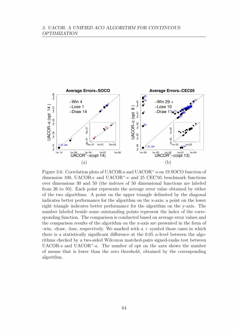
3. UACOR: A UNIFIED ACO ALGORITHM FOR CONTINUOUSOPTIMIZATION
1e−14 1e−09 1e−04 1e+01 1e+06
1e−
14
1e−
09
1e−
04
1e+
01
1e+
06
UACOR+−s(opt 14)
UA
CO
R−
s (
op
t 1
4 )
f_id_opt
2
3
8
1317
−Win 4
−Lose 1
−Draw 14
Average Errors−SOCO
5e−01 1e+01 5e+025e−
01
5e+
01
3
8
1317
1e−08 1e−05 1e−02 1e+01 1e+04
1e−
08
1e−
05
1e−
02
1e+
01
1e+
04
UACOR+−c(opt 13)
UA
CO
R−
c (
op
t 8
)
f_id_opt
3
4
6
7
8
9
1011
12
13
14
1516 171819202122232425
28
29
31
32
33
34
3536
37
38
39
404142 4344454647484950
−Win 29 +
−Lose 10
−Draw 11
Average Errors−CEC05
1e−02 1e+021e−
02
1e+
02
(a) (b)
Figure 3.6: Correlation plots of UACOR-s and UACOR+-s on 19 SOCO function ofdimension 100, UACOR-c and UACOR+-c and 25 CEC’05 benchmark functionsover dimensions 30 and 50 (the indexes of 50 dimensional functions are labeledfrom 26 to 50). Each point represents the average error value obtained by eitherof the two algorithms. A point on the upper triangle delimited by the diagonalindicates better performance for the algorithm on the x-axis; a point on the lowerright triangle indicates better performance for the algorithm on the y-axis. Thenumber labeled beside some outstanding points represent the index of the corre-sponding function. The comparison is conducted based on average error values andthe comparison results of the algorithm on the x-axis are presented in the form of-win, -draw, -lose, respectively. We marked with a + symbol those cases in whichthere is a statistically significant difference at the 0.05 α-level between the algo-rithms checked by a two-sided Wilcoxon matched-pairs signed-ranks test betweenUACOR-s and UACOR+-s. The number of opt on the axes shows the numberof means that is lower than the zero threshold, obtained by the correspondingalgorithm.
64

3.6 Summary
In this chapter, we proposed UACOR, a unified ant colony framework, that inte-
grates algorithmic components from three previous ACO algorithms for continuous
optimization problems, ACOR [Socha and Dorigo, 2008], DACOR [Leguizamon and
Coello, 2010] and IACOR-LS [Liao et al., 2011b]. The UACOR framework is flex-
ible and allows the instantiation of new ACO algorithms for continuous optimiza-
tion through the exploitation of automatic algorithm configuration techniques. In
fact, in this way we can obtain from the available algorithmic components new
ACO algorithms that have not been considered or tested before.
In the experimental part of the chapter, we have shown that the combina-
tion of a flexible, unified algorithm for continuous optimization and automatic
algorithm configuration tools can be instrumental for generating new, very high
performing algorithms for continuous optimization. We have configured UACOR
using Iterated F-Race [Birattari et al., 2010], an automatic algorithm configura-
tion technique implemented in the irace package [Lopez-Ibanez et al., 2011], on
small dimensional training functions taken from two well-known benchmark sets,
the SOCO and the CEC’05 benchmark sets, for continuous optimization. The
computational results showed that the tuned UACOR algorithms obtain better
performance on each of the benchmark sets than the tuned variants of the three
ACO algorithms that underly the UACOR framework, namely ACOR, DACOR and
IACOR-LS. Moreover, when UACOR is automatically configured for the SOCO
benchmark set, it performs better or competitive to all the recent 16 algorithms
benchmarked on this benchmark set; when configured for the CEC’05 benchmark
set, it performs competitive to IPOP-CMA-ES, the acknowledged state-of-the-art
algorithm on this benchmark set and also competitive or superior to other five
recent high-performance continuous optimizers that were evaluated on this bench-
mark set.
Finally we proposed UACOR+, a re-designed and improved UACOR that now
also includes the option of using CMA-ES as a local search. The computational
results showed that the tuned UACOR+ algorithms statistically significantly im-
prove ACOR, DACOR and IACOR-LS on each of the benchmark sets. When
UACOR+ is automatically configured for the SOCO benchmark set, it performs
statistically significantly better than 12 of the recent 16 algorithms benchmarked
on this benchmark set. When configured for the CEC’05 benchmark set, it per-
forms superior to IPOP-CMA-ES and statistically significantly better than other
five recent high-performance continuous optimizers that were evaluated on this
65

3. UACOR: A UNIFIED ACO ALGORITHM FOR CONTINUOUSOPTIMIZATION
benchmark set.
In summary, in this chapter we have proven the high potential ACO algorithms
have for continuous optimization and that automatic algorithm configuration has
a high potential also for the development of continuous optimizers out of algorithm
components. This should encourage also other researchers to apply such automatic
algorithm configuration techniques in the design of continuous optimizers.
66

Chapter 4
iCMAES-ILS: A cooperative competitive hybrid algo-rithm for continuous optimization
The development of algorithms for tackling difficult, high-dimensional continu-
ous optimization problems (e.g. high-dimensional CEC’05 benchmark functions
[Suganthan et al., 2005]) is a main research theme in population based heuris-
tic algorithms. While initially pure algorithm strategies have been tested exten-
sively [Hansen and Ostermeier, 1996, 2001, Karaboga and Basturk, 2007, Kennedy
and Eberhart, 1995, Socha and Dorigo, 2008, Storn and Price, 1997], in the past
few years most newly proposed algorithms that reach state-of-the-art performance
combine elements from different algorithmic techniques, that is, they are hybrid
algorithms. A popular class of hybrid approaches embeds local optimizers into
global optimizers. Several examples that follow this approach use the covariance
matrix adaptation evolution strategy (CMA-ES) [Hansen and Ostermeier, 1996,
2001, Hansen et al., 2003] as a local optimizer and embed it into a real-coded
steady state genetic algorithm (SSGA) [Molina et al., 2010a], particle swarm op-
timization (PSO) [Muller et al., 2009], differential evolution (DE) [Ghosh et al.,
2012] or into the UACOR framework as done in the previous chapter, Section 3.5.
Alternative approaches include the definition of algorithm portfolios [Gomes and
Selman, 2001, Huberman et al., 1997] or the exploitation of algorithm selection
techniques [Bischl et al., 2012, Rice, 1976]. Peng et al. [Peng et al., 2010] define a
portfolio of four algorithms and do report, on few classical benchmark functions,
some improvements over IPOP-CMA-ES [Auger and Hansen, 2005]. More recently,
algorithm selection is being explored as one possible way to improve upon state-
of-the-art algorithms. One common way is to define problem features and based
on the measured feature values to choose an algorithm for final execution. This
approach has been followed by [Bischl et al., 2012], where features for continuous
optimization problems taken from [Mersmann et al., 2011] have been exploited.
67

4. ICMAES-ILS: A COOPERATIVE COMPETITIVE HYBRID ALGORITHMFOR CONTINUOUS OPTIMIZATION
However, they conclude that the feature computation gives a significant overhead
leading to a situation that it may make this approach not advantageous.
In this chapter, we propose iCMAES-ILS, a structurally simple, hybrid al-
gorithm that loosely couples IPOP-CMA-ES with an iterated local search (ILS)
algorithm. The hybrid iCMAES-ILS algorithm consists of an initial competition
phase, in which IPOP-CMA-ES and the ILS algorithm compete for further execu-
tion in the deployment phase, where only one of the two algorithms is run until the
budget is exhausted. The initial competition phase features also a cooperative as-
pect between IPOP-CMA-ES and the ILS algorithm. In fact, first IPOP-CMA-ES
is run for a specific initial budget and the best solution found by IPOP-CMA-ES
is used to bias the acceptance decision in the ILS algorithm, which is run next for
a same initial budget as IPOP-CMA-ES.
We consider iCMAES-ILS to be a simple algorithm since the two algorithms
it is based upon can be seen as black boxes and the main design issue is on how
to interleave the execution of the two component algorithms. iCMAES-ILS is also
related to approaches for algorithm selection [Rice, 1976]. However, instead of
extracting sometimes complex problem features and then deciding upon which
algorithm to execute [Bischl et al., 2012], we use the performance of the two
component algorithms in an initial competition phase as the feature and then
directly employ the better one, thus, making again the design of iCMAES-ILS
very simple.
We also show that iCMAES-ILS is an effective algorithm that reaches (and
actually statistically significantly surpasses) state-of-the-art performance. As our
testbed, we use all 25 benchmark functions of 30 and 50 dimensions from the
CEC’05 benchmark [Suganthan et al., 2005]. We use this benchmark set to com-
pare iCMAES-ILS to its component algorithms, IPOP-CMA-ES and ILS, and also
to a number of alternative hybrids between IPOP-CMA-ES and ILS based on using
portfolios, interleaving the execution of IPOP-CMA-ES and ILS, and using ILS as
an improvement method between restarts of IPOP-CMA-ES. These comparisons
indicate that iCMAES-ILS reaches statistically significantly better performance
than almost all competitors and, thus, establishes our hybrid design as the most
performing one. Additional comparisons to two state-of-the-art CMA-ES hybrid
algorithms (MA-LSCh-CMA [Molina et al., 2010a] and PS-CMA-ES [Muller et al.,
2009]) further show statistically significantly better performance of iCMAES-ILS
over these competitors. In a final step, we tune iCMAES-ILS by applying irace
[Lopez-Ibanez et al., 2011] to examine the further performance improvements that
can be expected from a more careful fine-tuning of the algorithm parameters.
68

Overall, our experimental results establish iCMAES-ILS as a new state-of-the-art
algorithm for continuous optimization.
The chapter is organized as follows. Section 4.1 describes iCMAES-ILS. In
Section 4.2, we analyze, evaluate and compare iCMAES-ILS to results from the
literature. In Section 4.3, we further fine-tune iCMAES-ILS and examine the
further performance improvements. We end by some discussion and concluding
remarks in Sections 4.4 and 4.5.
4.1 iCMAES-ILS algorithm
The iCMAES-ILS algorithm build upon and extends IPOP-CMA-ES for continu-
ous optimization. The main details of the IPOP-CMA-ES algorithm have already
been described in Section 2.3.2 and we refer the reader to the details described
there. Next, we describe the ILS algorithm and then describe the hybrid iCMAES-
ILS algorithm.
4.1.1 ILS
Iterated local search [Lourenco et al., 2010] is a stochastic local search method
[Hoos and Stutzle, 2005] that iterates between improvements through local search
and solution perturbations that are used to define new promising starting solutions
for a local search. An additional acceptance criterion decides from which candidate
solution the search is continued. Recently, iterated local search has been applied
to solve continuous optimization problems [Gimmler, 2005, Kramer, 2010] showing
very promising results. For this chapter, we present a new iterated local search
algorithm (labeled as ILS), where a high-performing derivative-free local search
algorithm for continuous optimization, Mtsls1 [Tseng and Chen, 2008], is used.
The Mtsls1 local search was chosen since it is a crucial component of several high-
performing algorithms for continuous optimization [LaTorre et al., 2011, Liao et al.,
2011b]. Mtsls1 iteratively searches along dimensions one by one in a certain step
size. If one Mtsls1 iteration does not find an improvement in any of the dimensions,
the next Mtsls1 iteration halves the search step size. For more details, we refer
back to Chapter 2, Section 2.1.1, page 17. Algorithm 3 gives an outline of the
proposed ILS algorithm. For purposes that are explained later, we use two input
solutions, S and Sbest; the behavior of a standard ILS algorithm [Lourenco et al.,
2010] would be obtained by setting S = Sbest. In our ILS algorithm, local search is
first executed generating a new solution Snew. If Snew is better than the best-so-far
69

4. ICMAES-ILS: A COOPERATIVE COMPETITIVE HYBRID ALGORITHMFOR CONTINUOUS OPTIMIZATION
Algorithm 3 Outline of the ILS algorithmInput: Candidate solution S, Sbest and termination criterionOutput: the best found solution
while termination criterion is not satisfied doSnew ← LS (S, ss, LSIterations) /* Local search procedure */if f(Snew) < f(Sbest) thenS ← Snew
Sbest ← Snew
elseS ← Srand + r × (Sbest − Srand) /* Perturbation */
end ifend while
solution Sbest, Snew undergoes a refinement local search (that is, no perturbation
is applied before calling the next time the local search procedure). Otherwise, the
local search continues from a solution obtained by perturbation. The perturbation
uses information from Sbest. It is biased towards the best-so-far solution Sbest using
S = srand + r× (Sbest−Srand), where Srand is a random solution and r is a random
number chosen uniformly at random in [0, 1).
4.1.2 iCMAES-ILS
iCMAES-ILS is a hybrid of IPOP-CMA-ES and ILS. iCMAES-ILS consists of two
phases, competition and deployment. In the competition phase, IPOP-CMA-ES
and ILS start from the same initial solution and are sequentially executed with the
same budget of function evaluations, CompBudget. After the competition phase,
the one of the two that found the better solution is deployed for the remaining
budget. Specifically, if ILS finds a better solution than IPOP-CMA-ES, iCMAES-
ILS applies ILS for the remaining budget. Otherwise, iCMAES-ILS restarts IPOP-
CMA-ES from the best-so-far solution with its initial default parameter settings.
The restart of IPOP-CMA-ES is triggered by the end of the competition phase,
that is, not due to the internal termination criterion of IPOP-CMA-ES; as we
will show in Section 4.2, this external restart trigger is beneficial to iCMAES-ILS’
performance.
In iCMAES-ILS, the input Sbest of ILS is set to the best-so-far solution returned
by the IPOP-CMA-ES. Thus, the competition phase in iCMAES-ILS includes also
some aspect of cooperation between the two algorithms implemented through the
transfer of a candidate solution from IPOP-CMA-ES to ILS. The transferred can-
didate solution influences the search behavior of ILS by biasing the acceptance
decision and the perturbation. In an independent ILS algorithm, which we will
use as a reference for comparison, the input Sbest is set to the same as the input
70

Algorithm 4 Outline of iCMAES-ILSInput: Candidate solution S and termination criterion (TotalBudget)Output: the best found solutionCompBudget← compr × TotalBudgetSbest ← IPOP-CMA-ES (S, CompBudget)S′best ← ILS (S, Sbest, CompBudget)/* Heuristic deployment */if f(S′best < f(Sbest) then
ILS (S′best, S′best, TotalBudget−2×CompBudget) /* ILS found better solution than IPOP-
CMA-ES */else
IPOP-CMA-ES (Sbest, TotalBudget−2×CompBudget) /* IPOP-CMA-ES found better so-lution than ILS */
end if
Evaluate fitness values
Remark:If(ILS better) deploy ILS from best-so-far solutionElse restart IPOP-CMA-ES from best-so-far solution
Start from one solution
Transfer fitness value
Remark:The input Sbest of ILS is assigned to the best-so-far solution returned byIPOP-CMA-ES
Figure 4.1: A schematic view of iCMAES-ILS in the perspective of optimizationprocess.
candidate solution S. We set CompBudget= compr×TotalBudget, where Total-
Budget is the maximum number of function evaluations in each algorithm run. As
default, we use compr = 0.1. An outline and a schematic view of iCMAES-ILS is
given in Algorithm 4 and Fig. 4.1, respectively.
4.2 Algorithm analysis and evaluation
Experimental setup
Our test-suite consists of 25 CEC’05 benchmark functions (functions labeled as
fcec∗) of dimensions 30 and 50. We followed the protocol described in [Suganthan
et al., 2005] for the CEC’05 test-suite, that is, the maximum number of function
evaluations is 10 000×D. The investigated algorithms were independently run 25
71

4. ICMAES-ILS: A COOPERATIVE COMPETITIVE HYBRID ALGORITHMFOR CONTINUOUS OPTIMIZATION
Table 4.1: Given are the default parameter settings of iCMAES-ILS. (B − A) isthe size of the initial search interval. TotalBudget is the maximum number offunction evaluations.
Algorithm Components Parameter settings
IPOP-CMA-ES
Init pop size: λ0 = 4 + b3 ln(D)cParent size: µ = bλ/2c
Init step size: σ0 = 0.5× (B −A)IPOP factor: ipop = 2
stopTolFun = 10−12
stopTolFunHist = 10−20
stopTolX = 10−12
ILS LSIterations = 1.5×D
Competition Design compr = 0.1
times on each function. We report error values defined as f(S)−f(S∗), where S is
a candidate solution and S∗ is the optimal solution. Error values lower than 10−8
are clamped to 10−8, which is used as the zero threshold. To ensure that the final
solution obtained by iCMAES-ILS is inside the bounds, the bound constraints of
the benchmark functions are enforced by clamping the variable of each generated
solution that violates the bound constraints to the nearest value on the bounds
before evaluating a solution. Our analysis considers the average errors on each
function, and the distribution of the average errors on the CEC’05 benchmark
function set over dimensions 30 and 50. We apply the Friedman test at the 0.05
α-level to check whether the differences in the average rank values obtained by
multiple algorithms over the CEC’05 benchmark functions is statistically signifi-
cant. The parameter settings used for iCMAES-ILS are listed in Table 4.1. The
parameter settings of IPOP-CMA-ES and ILS in iCMAES-ILS are the same as the
default IPOP-CMA-ES and ILS algorithms, respectively.
4.2.1 Algorithm analysis: the role of ILS
As a first indication of performance, we present in Table 4.2 the average errors
by ILS, IPOP-CMA-ES, and iCMAES-ILS for 25 CEC’05 function of dimension
50. Interestingly, iCMAES-ILS obtains lower average errors than ILS and IPOP-
CMA-ES on most of the functions: iCMAES-ILS finds 19 lowest average error
values while ILS and IPOP-CMA-ES find 7 and 10, respectively. These results
indicate that iCMAES-ILS finds better results than its component algorithms,
that is, it shows some synergetic effect through the hybrid design.
Next, we analyze the role of ILS in iCMAES-ILS on the 18 benchmark functions
72

of dimension 50, where iCMAES-ILS obtained either a better or a worse average
error than IPOP-CMA-ES alone. On a per function basis, Fig. 4.2 shows the
development of the average error for IPOP-CMA-ES and iCMAES-ILS over the
number of function evaluations (also called SQT curves [Hoos and Stutzle, 2005]
for solution quality over time). The ILS phase in iCMAES-ILS is shown between
the two vertically dotted lines in the SQT curves for iCMAES-ILS. It is observed
that in functions fcec8, fcec12, fcec13, fcec14, fcec15, fcec21, fcec23, fcec25, where the
average error after the ILS execution is lower than after executing IPOP-CMA-ES,
iCMAES-ILS strongly improves upon IPOP-CMA-ES w.r.t. final average solution
quality. Only for functions fcec6, fcec9, the improvement by ILS does not lead to a
final improvement of iCMAES-ILS over IPOP-CMA-ES. For functions fcec4, fcec11,
fcec16, fcec17, fcec18, fcec22, ILS does not find any further improvement over IPOP-
CMA-ES. However, the external restart triggered through the end of the ILS phase
seems to be helpful, as indicated by the very good performance of iCMAES-ILS
w.r.t. IPOP-CMA-ES on these functions. Specially in functions fcec4 and fcec17,
we can observe that the external restart trigger obviously helps. In fact, on these
two functions IPOP-CMA-ES would not restart according to its internal restart
criterion and, thus, stagnate on high average error values. Only for functions fcec5,
fcec10, the restart trigger does not help. Table 4.3 summarizes our observations.
73
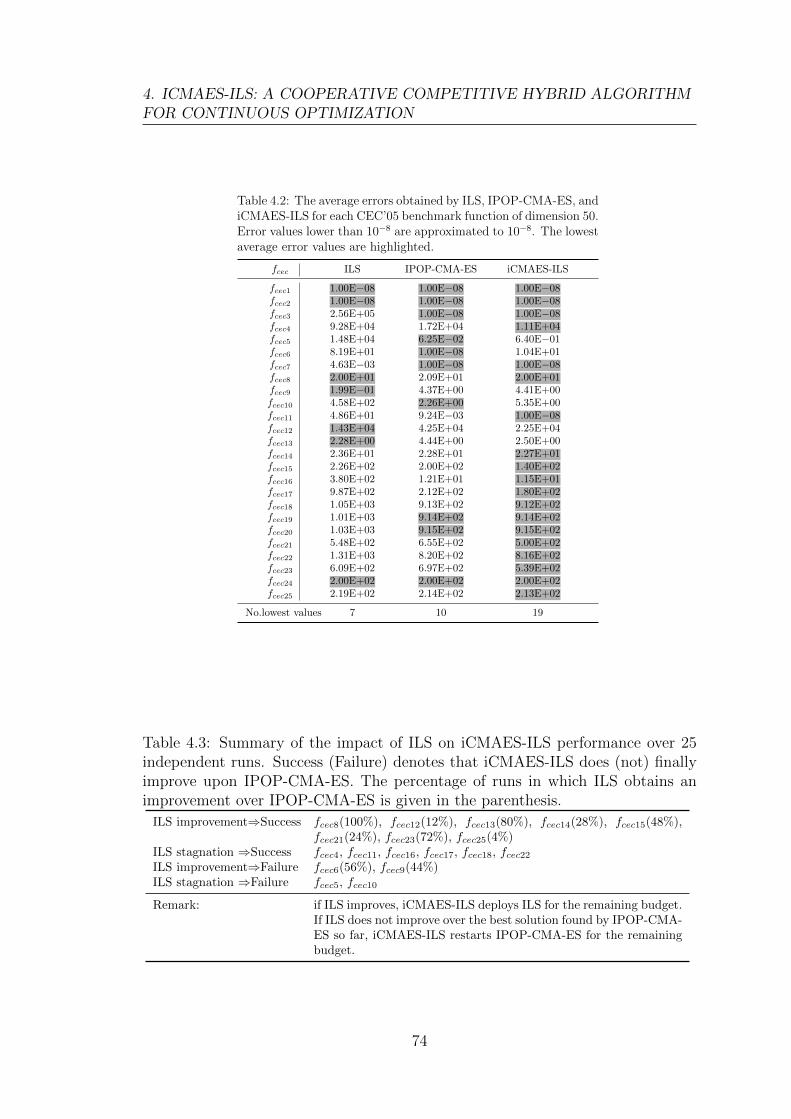
4. ICMAES-ILS: A COOPERATIVE COMPETITIVE HYBRID ALGORITHMFOR CONTINUOUS OPTIMIZATION
Table 4.2: The average errors obtained by ILS, IPOP-CMA-ES, andiCMAES-ILS for each CEC’05 benchmark function of dimension 50.Error values lower than 10−8 are approximated to 10−8. The lowestaverage error values are highlighted.
fcec ILS IPOP-CMA-ES iCMAES-ILS
fcec1 1.00E−08 1.00E−08 1.00E−08fcec2 1.00E−08 1.00E−08 1.00E−08fcec3 2.56E+05 1.00E−08 1.00E−08fcec4 9.28E+04 1.72E+04 1.11E+04fcec5 1.48E+04 6.25E−02 6.40E−01fcec6 8.19E+01 1.00E−08 1.04E+01fcec7 4.63E−03 1.00E−08 1.00E−08fcec8 2.00E+01 2.09E+01 2.00E+01fcec9 1.99E−01 4.37E+00 4.41E+00fcec10 4.58E+02 2.26E+00 5.35E+00fcec11 4.86E+01 9.24E−03 1.00E−08fcec12 1.43E+04 4.25E+04 2.25E+04fcec13 2.28E+00 4.44E+00 2.50E+00fcec14 2.36E+01 2.28E+01 2.27E+01fcec15 2.26E+02 2.00E+02 1.40E+02fcec16 3.80E+02 1.21E+01 1.15E+01fcec17 9.87E+02 2.12E+02 1.80E+02fcec18 1.05E+03 9.13E+02 9.12E+02fcec19 1.01E+03 9.14E+02 9.14E+02fcec20 1.03E+03 9.15E+02 9.15E+02fcec21 5.48E+02 6.55E+02 5.00E+02fcec22 1.31E+03 8.20E+02 8.16E+02fcec23 6.09E+02 6.97E+02 5.39E+02fcec24 2.00E+02 2.00E+02 2.00E+02fcec25 2.19E+02 2.14E+02 2.13E+02
No.lowest values 7 10 19
Table 4.3: Summary of the impact of ILS on iCMAES-ILS performance over 25independent runs. Success (Failure) denotes that iCMAES-ILS does (not) finallyimprove upon IPOP-CMA-ES. The percentage of runs in which ILS obtains animprovement over IPOP-CMA-ES is given in the parenthesis.
ILS improvement⇒Success fcec8(100%), fcec12(12%), fcec13(80%), fcec14(28%), fcec15(48%),fcec21(24%), fcec23(72%), fcec25(4%)
ILS stagnation ⇒Success fcec4, fcec11, fcec16, fcec17, fcec18, fcec22ILS improvement⇒Failure fcec6(56%), fcec9(44%)ILS stagnation ⇒Failure fcec5, fcec10
Remark: if ILS improves, iCMAES-ILS deploys ILS for the remaining budget.If ILS does not improve over the best solution found by IPOP-CMA-ES so far, iCMAES-ILS restarts IPOP-CMA-ES for the remainingbudget.
74

0e+00 1e+05 2e+05 3e+05 4e+05 5e+05
2e+
04
5e+
04
1e+
05
Function evaluations
Ave
rag
e e
rro
rs o
f fitn
ess v
alu
es
2e+
04
5e+
04
1e+
05
IPOP−CMA−ES
iCMAES−ILS
f4−50D
0e+00 1e+05 2e+05 3e+05 4e+05 5e+05
1e−
01
1e+
01
1e+
03
1e+
05
Function evaluations
Ave
rag
e e
rro
rs o
f fitn
ess v
alu
es
1e−
01
1e+
01
1e+
03
1e+
05
IPOP−CMA−ES
iCMAES−ILS
f5−50D
0e+00 1e+05 2e+05 3e+05 4e+05 5e+051e−
08
1e−
03
1e+
02
1e+
07
1e+
12
Function evaluations
Ave
rag
e e
rro
rs o
f fitn
ess v
alu
es
1e−
08
1e−
03
1e+
02
1e+
07
1e+
12
IPOP−CMA−ES
iCMAES−ILS
f6−50D
0e+00 1e+05 2e+05 3e+05 4e+05 5e+05
20.0
20.5
21.0
21.5
Function evaluations
Ave
rag
e e
rro
rs o
f fitn
ess v
alu
es
20.0
20.5
21.0
21.5
IPOP−CMA−ES
iCMAES−ILS
f8−50D
0e+00 1e+05 2e+05 3e+05 4e+05 5e+05
510
20
50
100
Function evaluations
Ave
rag
e e
rro
rs o
f fitn
ess v
alu
es
510
20
50
100
IPOP−CMA−ES
iCMAES−ILS
f9−50D
0e+00 1e+05 2e+05 3e+05 4e+05 5e+05
25
20
50
200
1000
Function evaluations
Ave
rag
e e
rro
rs o
f fitn
ess v
alu
es
25
20
50
200
1000
IPOP−CMA−ES
iCMAES−ILS
f10−50D
0e+00 1e+05 2e+05 3e+05 4e+05 5e+051e−
08
1e−
05
1e−
02
1e+
01
Function evaluations
Ave
rag
e e
rro
rs o
f fitn
ess v
alu
es
1e−
08
1e−
05
1e−
02
1e+
01 IPOP−CMA−ES
iCMAES−ILS
f11−50D
0e+00 1e+05 2e+05 3e+05 4e+05 5e+05
4e+
04
6e+
04
1e+
05
Function evaluations
Ave
rag
e e
rro
rs o
f fitn
ess v
alu
es
4e+
04
6e+
04
1e+
05
IPOP−CMA−ES
iCMAES−ILS
f12−50D
0e+00 1e+05 2e+05 3e+05 4e+05 5e+05
46
810
Function evaluations
Ave
rag
e e
rro
rs o
f fitn
ess v
alu
es
46
810
IPOP−CMA−ES
iCMAES−ILS
f13−50D
0e+00 1e+05 2e+05 3e+05 4e+05 5e+05
22.8
23.0
23.2
23.4
Function evaluations
Ave
rag
e e
rro
rs o
f fitn
ess v
alu
es
22.8
23.0
23.2
23.4
IPOP−CMA−ES
iCMAES−ILS
f14−50D
0e+00 1e+05 2e+05 3e+05 4e+05 5e+05
140
160
180
200
240
Function evaluations
Ave
rag
e e
rro
rs o
f fitn
ess v
alu
es
140
160
180
200
240
IPOP−CMA−ES
iCMAES−ILS
f15−50D
0e+00 1e+05 2e+05 3e+05 4e+05 5e+05
20
50
100
Function evaluations
Ave
rag
e e
rro
rs o
f fitn
ess v
alu
es
20
50
100
IPOP−CMA−ES
iCMAES−ILS
f16−50D
0e+00 1e+05 2e+05 3e+05 4e+05 5e+05
180
190
200
210
220
230
Function evaluations
Ave
rag
e e
rro
rs o
f fitn
ess v
alu
es
180
190
200
210
220
230
IPOP−CMA−ES
iCMAES−ILS
f17−50D
0e+00 1e+05 2e+05 3e+05 4e+05 5e+05
915
920
925
930
Function evaluations
Ave
rag
e e
rro
rs o
f fitn
ess v
alu
es
915
920
925
930
IPOP−CMA−ES
iCMAES−ILS
f18−50D
0e+00 1e+05 2e+05 3e+05 4e+05 5e+05
600
800
1200
1600
Function evaluations
Ave
rag
e e
rro
rs o
f fitn
ess v
alu
es
600
800
1200
1600
IPOP−CMA−ES
iCMAES−ILS
f21−50D
0e+00 1e+05 2e+05 3e+05 4e+05 5e+05
820
840
860
880
900
920
Function evaluations
Ave
rag
e e
rro
rs o
f fitn
ess v
alu
es
820
840
860
880
900
920
IPOP−CMA−ES
iCMAES−ILS
f22−50D
0e+00 1e+05 2e+05 3e+05 4e+05 5e+05
600
800
1200
1600
Function evaluations
Ave
rag
e e
rro
rs o
f fitn
ess v
alu
es
600
800
1200
1600
IPOP−CMA−ES
iCMAES−ILS
f23−50D
0e+00 1e+05 2e+05 3e+05 4e+05 5e+05
213.5
214.0
214.5
215.0
Function evaluations
Ave
rag
e e
rro
rs o
f fitn
ess v
alu
es
213.5
214.0
214.5
215.0
IPOP−CMA−ES
iCMAES−ILS
f25−50D
Figure 4.2: SQT curves of IPOP-CMA-ES and iCMAES-ILS. The ILS phase iniCMAES-ILS is shown between the two vertically dotted lines.
75

4. ICMAES-ILS: A COOPERATIVE COMPETITIVE HYBRID ALGORITHMFOR CONTINUOUS OPTIMIZATION
4.2.2 Performance evaluation of iCMAES-ILS
As a next step, we compare the performance of iCMAES-ILS to a number of al-
ternative possibilities that include using ILS and IPOP-CMA-ES as standalone
algorithms, defining combinations between IPOP-CMA-ES and ILS, and algo-
rithms that integrate CMA-ES into other global optimization methods. We next
introduce the other combinations of ILS and IPOP-CMA-ES and the CMA-ES
hybrids.
1. We designed three different combinations between IPOP-CMA-ES and
ILS. They are labeled as iCMAES-ILS-portfolio, iCMAES-ILS-relay and
iCMAES-LTH-ILS, respectively. iCMAES-ILS-portfolio is a portfolio-based
algorithm, in which ILS and IPOP-CMA-ES run in parallel each with half
of TotalBudget. iCMAES-ILS-relay follows a high-level relay hybrid scheme
[Talbi, 2002], in which ILS relays IPOP-CMA-ES in a number of cycles, in
which ILS and IPOP-CMA-ES use in each run relayP × TotalBudget eval-
uations until the total budget is exhausted. iCMAES-LTH-ILS follows a
low-level teamwork hybrid (LTH) scheme [Talbi, 2002], where ILS is embed-
ded as a local search procedure before IPOP-CMA-ES restarts; ILS uses in
each of its runs lsP×TotalBudget evaluations. We test values of relayP and
lsP ∈ 0.01, 0, 025, 0.05, 0.1, 0.25, 0.5. A schematic view of iCMAES-ILS-
portfolio, iCMAES-ILS-relay and iCMAES-LTH-ILS is shown in Fig.4.3.
2. We compare iCMAES-ILS also to results obtained from two state-of-the-art
algorithms, MA-LSCh-CMA [Molina et al., 2010a] and PS-CMA-ES [Muller
et al., 2009], which use CMA-ES as a local search method and to the re-
sults of IPOP-CMA-ES-cec05 [Auger and Hansen, 2005]. In MA-LSCh-CMA
[Molina et al., 2010a], CMA-ES is used as a local search procedure, and
SSGA [Herrera et al., 1998] is specifically designed for diversification. In PS-
CMA-ES [Muller et al., 2009], multiple instances of CMA-ES concurrently
explore different search space regions and exchange information as the par-
ticle swarm does, then adapt the search direction and distribution in each
CMA-ES instance. Recall that IPOP-CMA-ES-cec05 are the results for the
CEC’05 benchmark functions taken from [Auger and Hansen, 2005]; IPOP-
CMA-ES-cec05 is a Matlab version of IPOP-CMA-ES and it handles bound
constraints by an approach based on penalty functions, which is described
in [Hansen et al., 2009c].
76

ILS
iCMAES1. iCMAES-ILS-Portfolio
ILS
iCMAES2. iCMAES-ILS-Relay iCMAES
ILS
iCMAES3. iCMAES-LTH-ILS
ILSILS
Before restart
Figure 4.3: A schematic view of three combinations of IPOP-CMA-ES and ILS weused as comparison to our hybrid design. The empty points denote solutions thatare transferred between IPOP-CMA-ES and ILS.
Table 4.4 gives average algorithm rankings on the CEC’05 benchmark function
set over dimensions 30 and 50. We carry out a Friedman test at the 0.05 α-level
to check for the significance of the differences between the best ranked algorithm
and the others. The results of the Friedman tests are given in the last column of
Table 4.4. ∆Rα is the minimum significant difference between the algorithms. The
numbers in parenthesis are the differences of the sum of ranks relative to the best
algorithm. Algorithms that are significantly worse than the best ranked algorithm
are indicated in bold face. The experimental results identify iCMAES-ILS as the
best ranked algorithm. In particular, iCMAES-ILS performs statistically signifi-
cantly better than (i) its component algorithms IPOP-CMA-ES and ILS; (ii) most
other hybrid algorithms including iCMAES-ILS-portfolio, the worst three ranked
iCMAES-ILS-relay variants and all variants of iCMAES-LTH-ILS; (iii) various al-
gorithms from literature, namely MA-LSCh-CMA [Molina et al., 2010a], PS-CMA-
ES [Muller et al., 2009] and IPOP-CMA-ES-cec05 [Auger and Hansen, 2005]. No
statistically significant difference was found between iCMAES-ILS and the best
three ranked iCMAES-ILS-relay variants, which indicates that iCMAES-ILS-relay
with few cycles reaches promising performance.
The detailed average error values of MA-LSCh-CMA, PS-CMA-ES, IPOP-
CMA-ES-cec05 and iCMAES-ILS are given in Table 4.8 (results for the other
algorithms are given in the supplementary material http://iridia.ulb.ac.be/
supp/IridiaSupp2012-017. It is observed that on the uni-model functions (fcec1
to fcec5) over dimension 30 and 50, iCMAES-ILS performs better than IPOP-
77
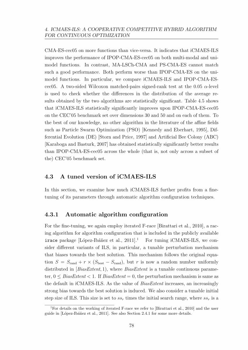
4. ICMAES-ILS: A COOPERATIVE COMPETITIVE HYBRID ALGORITHMFOR CONTINUOUS OPTIMIZATION
CMA-ES-cec05 on more functions than vice-versa. It indicates that iCMAES-ILS
improves the performance of IPOP-CMA-ES-cec05 on both multi-modal and uni-
model functions. In contrast, MA-LSCh-CMA and PS-CMA-ES cannot match
such a good performance. Both perform worse than IPOP-CMA-ES on the uni-
model functions. In particular, we compare iCMAES-ILS and IPOP-CMA-ES-
cec05. A two-sided Wilcoxon matched-pairs signed-rank test at the 0.05 α-level
is used to check whether the differences in the distribution of the average re-
sults obtained by the two algorithms are statistically significant. Table 4.5 shows
that iCMAES-ILS statistically significantly improves upon IPOP-CMA-ES-cec05
on the CEC’05 benchmark set over dimensions 30 and 50 and on each of them. To
the best of our knowledge, no other algorithm in the literature of the affine fields
such as Particle Swarm Optimization (PSO) [Kennedy and Eberhart, 1995], Dif-
ferential Evolution (DE) [Storn and Price, 1997] and Artificial Bee Colony (ABC)
[Karaboga and Basturk, 2007] has obtained statistically significantly better results
than IPOP-CMA-ES-cec05 across the whole (that is, not only across a subset of
the) CEC’05 benchmark set.
4.3 A tuned version of iCMAES-ILS
In this section, we examine how much iCMAES-ILS further profits from a fine-
tuning of its parameters through automatic algorithm configuration techniques.
4.3.1 Automatic algorithm configuration
For the fine-tuning, we again employ iterated F-race [Birattari et al., 2010], a rac-
ing algorithm for algorithm configuration that is included in the publicly available
irace package [Lopez-Ibanez et al., 2011].1 For tuning iCMAES-ILS, we con-
sider different variants of ILS, in particular, a tunable perturbation mechanism
that biases towards the best solution. This mechanism follows the original equa-
tion S = Srand + r × (Sbest − Srand), but r is now a random number uniformly
distributed in [BiasExtent, 1), where BiasExtent is a tunable continuous parame-
ter, 0 ≤ BiasExtent < 1. If BiasExtent = 0, the perturbation mechanism is same as
the default in iCMAES-ILS. As the value of BiasExtent increases, an increasingly
strong bias towards the best solution is induced. We also consider a tunable initial
step size of ILS. This size is set to ssr times the initial search range, where ssr is a
1For details on the working of iterated F-race we refer to [Birattari et al., 2010] and the userguide in [Lopez-Ibanez et al., 2011]. See also Section 2.4.1 for some more details.
78

Table 4.4: The average ranks with respect to the average error values are given.The Friedman test at significance level α = 0.05 is used. ∆Rα is the minimumsignificant difference 95.05. The numbers in parenthesis are the difference of thesum of ranks relative to the best algorithm iCMAES-ILS. Algorithms that aresignificantly different from iCMAES-ILS are indicated in bold face.
Algorithms Average Rank (∆R)
Proposed iCMAES-ILS 7.28 (0)
Component algorithmsIPOP-CMA-ES 9.79 (125.5)ILS 14.39 (355.5)
Other hybrids
iCMAES-ILS-portfolio 9.29 (100.5)
iCMAES-ILS-relay-025 8.15 (43.5)iCMAES-ILS-relay-01 8.52 (62.0)iCMAES-ILS-relay-05 8.69 (70.5)iCMAES-ILS-relay-0025 9.68 (120.0)iCMAES-ILS-relay-005 9.86 (129.0)iCMAES-ILS-relay-001 11.63 (217.5)
iCMAES-LTH-ILS-025 9.46 (109.0)iCMAES-LTH-ILS-01 9.70 (121.0)iCMAES-LTH-ILS-005 9.78 (125.0)iCMAES-LTH-ILS-05 9.90 (131.0)iCMAES-LTH-ILS-0025 10.28 (150.0)iCMAES-LTH-ILS-001 10.33 (152.5)
LiteraturePS-CMA-ES 9.95 (133.5)IPOP-CMA-ES-cec05 11.53 (212.5)MA-LSCh-CMA 11.79 (225.5)
tunable continuous parameter, 0 < ssr ≤ 1. In total, we expose eleven parameters
that directly control internal parameters of iCMAES-ILS. These eleven parame-
ters are given in Table 4.7, together with the internal parameter of iCMAES-ILS
controlled by each of them, their default value and the range considered for tuning.
The setting of iterated F-race we used are the default [Lopez-Ibanez et al.,
2011]. The budget of each run of iterated F-race is set to 5 000 runs of iCMAES-
ILS. The performance measure is the fitness error value of each instance. Iterated
F-race handles two parameter types of iCMAES-ILS, continuous (r) and ordinal
(o). The inputs are the parameter ranges given in Table 4.7 and a set of training
instances.
As the training instances, we follow [Liao et al., 2013a] and consider a separa-
tion between training and test set to prevent the bias of the results due to poten-
tially overtuning iCMAES-ILS. We use the 10-dimensional benchmark functions
from the recent special issue of the Soft Computing journal (labeled as SOCO)
[Herrera et al., 2010, Lozano et al., 2011]. This SOCO benchmark set consists of
79

4. ICMAES-ILS: A COOPERATIVE COMPETITIVE HYBRID ALGORITHMFOR CONTINUOUS OPTIMIZATION
Table 4.5: The numbers in parenthesis represent the number of times IPOP-CMA-ES-cec05 is better, equal or worse, respectively, compared to iCMAES-ILS. Error values lower than 10−8 are approximated to 10−8.
IPOP-CMA-ES-cec05 vs iCMAES-ILS
Dim 30 by fcec: (4, 6, 15)† Dim 50 by fcec: (6, 4, 15)† Total by fcec: (10, 10, 30)†
† denotes a significant difference over the distribution of average errors between IPOP-CMA-ES-05 and iCMAES-ILS by a two-sided Wilcoxon matched-pairs signed-ranks test at the0,05 α-level.
19 functions. Four of these functions are the same as in the CEC’05 benchmark
set and are therefore removed from the training set. The training functions are
then sampled in a random order from all possible such functions. The number of
function evaluations of each run is equal to 5 000×D according to the termination
criteria in the definition of the SOCO benchmark set.
The tuned settings of iCMAES-ILS are presented in the last column of Table 4.7
and we label the tuned iCMAES-ILS as iCMAES-ILSt. The tuned parameter set-
tings of the IPOP-CMA-ES component imply a larger exploration at the beginning
of the search than in the default settings; the tuned parameter setting of the ILS
component imply a shorter local search, a larger initial step size and a slightly
stronger bias by the perturbation than in the default version.
4.3.2 Performance evaluation of iCMAES-ILSt
We apply iCMAES-ILSt to the CEC’05 benchmark functions of 30 and 50 di-
mensions as described in the experimental setup in Section 4.2 and compare its
results to iCMAES-ILS, a tuned ILS (labeled as ILSt) and a tuned IPOP-CMA-
ES [Liao et al., 2013a] (labeled as IPOP-CMA-ESt). The parameters and the
parameter ranges considered for tuning ILS and IPOP-CMA-ES as well as the
tuning setup and effort is the same as for tuning iCMAES-ILS. The parame-
ters of ILSt and IPOP-CMA-ESt are given in the supplementary information
pages http://iridia.ulb.ac.be/supp/IridiaSupp2012-017. Table 4.6 sum-
marizes the average ranking obtained by iCMAES-ILS, ILSt, IPOP-CMA-ESt and
iCMAES-ILSt. A Friedman test at the 0.05 α-level is used to check for the sig-
nificance of the differences between the best ranked algorithm iCMAES-ILSt and
the other algorithms. We find that iCMAES-ILSt is statistically significantly bet-
ter than ILSt and IPOP-CMA-ESt; iCMAES-ILSt also statistically significantly
improves upon iCMAES-ILS. The detailed average error values obtained by ILSt,
IPOP-CMA-ESt, iCMAES-ILS and iCMAES-ILSt are listed in Table 4.9. These
80

results further indicate the high performance that is reached by the design of
iCMAES-ILS and they also show the further improvement obtained through au-
tomatic algorithm configuration.
Table 4.6: The average ranks with respect to the average error values are given.The Friedman test at significance level α = 0.05 is used. ∆Rα are the minimumsignificant difference 13.24 for dimension 30 (left table) and 13.74 for dimension50 (right table), respectively. The numbers in parenthesis are the difference of thesum of ranks relative to the best algorithm iCMAES-ILSt. Algorithms that aresignificantly different from iCMAES-ILSt are indicated in bold face.
Dim=30 Algorithms Average Rank (∆R)
iCMAES-ILSt 1.82 (0)iCMAES-ILS 2.36 (13.5)IPOP-CMA-ESt 2.38 (14.0)ILSt 3.44 (40.5)
Dim=50 Algorithms Average Rank (∆R)
iCMAES-ILSt 1.80 (0)IPOP-CMA-ESt 2.38 (14.5)iCMAES-ILS 2.44 (16.0)ILSt 3.38 (39.5)
81

4. ICMAES-ILS: A COOPERATIVE COMPETITIVE HYBRID ALGORITHMFOR CONTINUOUS OPTIMIZATION
Tab
le4.7:
Param
etersth
athave
been
consid
eredfor
tunin
g.G
ivenare
the
defau
ltvalu
esof
the
param
etersan
dth
eran
gesw
econ
sidered
fortu
nin
g.T
he
lastcolu
mn
isth
etu
ned
param
etersettin
gs.A
lgorithm
Com
pon
ents
Para
mete
rIn
tern
al
para
mete
rD
efa
ult
Ran
ge
Tu
ned
IPO
P-C
MA
-ES
aIn
itp
opsize:
λ0
=4
+ba
ln(D
)c3
r[1,1
0]9.68
7b
Paren
tsize:
µ=bλ/bc
2r
[1,5
]1.6
14c
Init
stepsize:
σ0
=c·(B
−A
)0.5
r(0,1]
0.68
25d
IPO
Pfa
ctor:
ipop
=d
2r
[1,4
]3.2
45e
stopTolFun
=10e
−12
r[−
20,−
6]
−9.02
3f
stopTolFunHist
=10f
−20
r[−
20,−
6]
−10.8
2g
stopTolX
=10g
−12
r[−
20,−
6]
−16.2
6
ILS
irLSItera
tions
=ir ×
D1.5
o(1,1
.25,1.5
,1.75,2)
1ssr
ss=
ssr ×
(B−A
)0.5
r(0,1]
0.67
03
biase
BiasE
xtent
=biase
0r
[0,1)0.01
910
Com
petition
Design
compr
CompBudget
=com
pr ×
Tota
lBudget
0.1o
(0.0
5,0.1,0.15,0
.2,0.25,0.3
)0.1
5
82

Table 4.8: The average errors obtained by IPOP-CMA-ES-CEC05, MA-LSch-CMA, PS-CMA-ES andiCMAES-ILS for each CEC’05 function. Error values lower than 10−8 are approximated to 10−8. Thelowest average errors values are highlighted.
Dim fcec IPOP-CMA-ES-CEC05 MA-LSch-CMA PS-CMA-ES iCMAES-ILS
30 Dim
fcec1 1.00E−08 1.00E−08 1.00E−08 1.00E−08fcec2 1.00E−08 1.00E−08 1.00E−08 1.00E−08fcec3 1.00E−08 2.75E+04 2.96E+04 1.00E−08fcec4 1.11E+04 3.02E+02 4.56E+03 1.74E+02fcec5 1.00E−08 1.26E+03 2.52E+01 1.00E−08fcec6 1.00E−08 1.12E+00 1.15E+01 8.67E+00fcec7 1.00E−08 1.75E−02 1.00E−08 1.00E−08fcec8 2.01E+01 2.00E+01 2.00E+01 2.00E+01fcec9 9.38E−01 1.00E−08 8.76E−01 7.16E−01fcec10 1.65E+00 2.25E+01 5.57E−01 3.10E+00fcec11 5.48E+00 2.15E+01 7.10E+00 1.87E−02fcec12 4.43E+04 1.67E+03 8.80E+02 2.60E+03fcec13 2.49E+00 2.03E+00 2.05E+00 1.41E+00fcec14 1.29E+01 1.25E+01 1.24E+01 1.30E+01fcec15 2.08E+02 3.00E+02 1.37E+02 1.36E+02fcec16 3.50E+01 1.26E+02 1.59E+01 1.48E+01fcec17 2.91E+02 1.83E+02 9.15E+01 2.11E+02fcec18 9.04E+02 8.98E+02 9.05E+02 8.96E+02fcec19 9.04E+02 9.01E+02 8.85E+02 8.96E+02fcec20 9.04E+02 8.96E+02 9.05E+02 8.96E+02fcec21 5.00E+02 5.12E+02 5.00E+02 5.00E+02fcec22 8.03E+02 8.80E+02 8.43E+02 8.12E+02fcec23 5.34E+02 5.34E+02 5.34E+02 5.33E+02fcec24 9.10E+02 2.00E+02 2.00E+02 2.00E+02fcec25 2.11E+02 2.14E+02 2.10E+02 2.03E+02
50 Dim
fcec1 1.00E−08 1.00E−08 1.00E−08 1.00E−08fcec2 1.00E−08 3.06E−02 7.36E−06 1.00E−08fcec3 1.00E−08 3.21E+04 9.10E+04 1.00E−08fcec4 4.68E+05 3.23E+03 2.17E+04 1.11E+04fcec5 2.85E+00 2.69E+03 1.79E+03 6.40E−01fcec6 1.00E−08 4.10E+00 2.91E+01 1.04E+01fcec7 1.00E−08 5.40E−03 1.00E−08 1.00E−08fcec8 2.01E+01 2.00E+01 2.00E+01 2.00E+01fcec9 1.39E+00 1.00E−08 5.45E+00 4.41E+00fcec10 1.72E+00 5.01E+01 5.33E+00 5.35E+00fcec11 1.17E+01 4.13E+01 1.59E+01 1.00E−08fcec12 2.27E+05 1.39E+04 6.90E+03 2.25E+04fcec13 4.59E+00 3.15E+00 4.15E+00 2.50E+00fcec14 2.29E+01 2.22E+01 2.15E+01 2.27E+01fcec15 2.04E+02 3.72E+02 1.25E+02 1.40E+02fcec16 3.09E+01 6.90E+01 1.62E+01 1.15E+01fcec17 2.34E+02 1.47E+02 9.13E+01 1.80E+02fcec18 9.13E+02 9.41E+02 8.70E+02 9.12E+02fcec19 9.12E+02 9.38E+02 9.13E+02 9.14E+02fcec20 9.12E+02 9.28E+02 9.09E+02 9.15E+02fcec21 1.00E+03 5.00E+02 6.62E+02 5.00E+02fcec22 8.05E+02 9.14E+02 8.63E+02 8.16E+02fcec23 1.01E+03 5.39E+02 8.12E+02 5.39E+02fcec24 9.55E+02 2.00E+02 2.00E+02 2.00E+02fcec25 2.15E+02 2.21E+02 2.14E+02 2.13E+02
No.lowest values 16 13 21 30
83

4. ICMAES-ILS: A COOPERATIVE COMPETITIVE HYBRID ALGORITHMFOR CONTINUOUS OPTIMIZATION
Table 4.9: The average errors obtained by ILSt, IPOP-CMA-ESt, iCMAES-ILS and iCMAES-ILSt for each CEC’05 function. Error values lower than 10−8 are approximated to 10−8. Thelowest average errors values are highlighted.
Dim fcec ILSt IPOP-CMA-ESt iCMAES-ILS iCMAES-ILSt
30 Dim
fcec1 1.00E−08 1.00E−08 1.00E−08 1.00E−08fcec2 1.00E−08 1.00E−08 1.00E−08 1.00E−08fcec3 2.13E+05 1.00E−08 1.00E−08 1.00E−08fcec4 2.25E+04 1.00E−08 1.74E+02 1.00E−08fcec5 7.01E+03 1.00E−08 1.00E−08 1.00E−08fcec6 7.80E+01 1.00E−08 8.67E+00 1.00E−08fcec7 1.18E−02 1.00E−08 1.00E−08 1.00E−08fcec8 2.00E+01 2.08E+01 2.00E+01 2.00E+01fcec9 1.00E−08 1.99E+00 7.16E−01 5.70E−01fcec10 1.42E+02 1.59E+00 3.10E+00 1.63E+00fcec11 2.43E+01 5.09E−05 1.87E−02 4.08E−02fcec12 1.91E+03 4.22E+02 2.60E+03 6.11E+02fcec13 1.16E+00 2.53E+00 1.41E+00 1.69E+00fcec14 1.39E+01 1.10E+01 1.30E+01 1.16E+01fcec15 2.80E+02 2.00E+02 1.36E+02 1.16E+02fcec16 2.76E+02 1.11E+01 1.48E+01 1.18E+01fcec17 4.14E+02 2.08E+02 2.11E+02 1.67E+02fcec18 9.90E+02 9.04E+02 8.96E+02 8.96E+02fcec19 9.81E+02 9.04E+02 8.96E+02 8.96E+02fcec20 9.92E+02 9.04E+02 8.96E+02 8.96E+02fcec21 5.52E+02 5.00E+02 5.00E+02 4.89E+02fcec22 1.17E+03 8.17E+02 8.12E+02 8.11E+02fcec23 5.34E+02 5.34E+02 5.33E+02 5.33E+02fcec24 2.00E+02 2.00E+02 2.00E+02 2.00E+02fcec25 2.10E+02 2.09E+02 2.03E+02 2.02E+02
50 Dim
fcec1 1.00E−08 1.00E−08 1.00E−08 1.00E−08fcec2 1.00E−08 1.00E−08 1.00E−08 1.00E−08fcec3 2.92E+05 1.00E−08 1.00E−08 1.00E−08fcec4 8.45E+04 1.00E−08 1.11E+04 1.00E−08fcec5 1.35E+04 1.00E−08 6.40E−01 1.00E−08fcec6 3.75E+01 1.00E−08 1.04E+01 1.01E+01fcec7 4.04E−03 1.00E−08 1.00E−08 1.00E−08fcec8 2.00E+01 2.10E+01 2.00E+01 2.00E+01fcec9 1.00E−08 4.18E+00 4.41E+00 2.11E+00fcec10 4.06E+02 2.71E+00 5.35E+00 2.43E+00fcec11 4.78E+01 6.03E−02 1.00E−08 1.13E−01fcec12 9.60E+03 4.69E+03 2.25E+04 4.24E+03fcec13 1.92E+00 4.70E+00 2.50E+00 2.72E+00fcec14 2.37E+01 2.09E+01 2.27E+01 2.12E+01fcec15 2.92E+02 2.00E+02 1.40E+02 1.20E+02fcec16 3.33E+02 5.34E+00 1.15E+01 5.26E+00fcec17 7.01E+02 6.36E+01 1.80E+02 4.42E+01fcec18 9.89E+02 9.13E+02 9.12E+02 9.06E+02fcec19 9.80E+02 9.13E+02 9.14E+02 9.10E+02fcec20 1.01E+03 9.13E+02 9.15E+02 9.10E+02fcec21 5.60E+02 7.05E+02 5.00E+02 5.32E+02fcec22 1.33E+03 8.19E+02 8.16E+02 8.23E+02fcec23 5.67E+02 7.30E+02 5.39E+02 5.39E+02fcec24 2.00E+02 2.00E+02 2.00E+02 2.00E+02fcec25 2.20E+02 2.13E+02 2.13E+02 2.13E+02
No.lowest values 12 23 22 36
84

4.4 Comparisions of iCMAES-ILS and UACOR+
As a final step, we compare iCMAES-ILS to UACOR+, the UACOR version that
included CMA-ES as a local search as proposed in Chapter 3. For this analysis, we
consider the average errors on each function, and the distribution of the average
errors. For a fair comparison, the same tuning setup and effort is considered for
obtaining the parameter settings.
We first re-tuned UACOR+-c allowing this time also to tune the parameters of
CMA-ES (resulting in a configuration labeled as UACOR+-ct). For this, we used
tuning setup and effort to be the same as tuning iCMAES-ILS to result in iCMAES-
ILSt. The parameter values of the tuned CMA-ES in UACOR+-ct are popula-
tion size λ = 4 + b9.600 ln(D)c, parent size µ = bλ/1.452c, stopTolFun10−8.854,
stopTolFunHist = 10−9.683 and stopTolX = 10−12.55. These parameter values are
derived from Liao et al. [2013a]. The initial step size of CMA-ES in UACOR+-ct
is defined adaptively as in UACOR+, not a fixed parameter value. We then ran
UACOR+-ct on the CEC’05 benchmark functions of dimensions 30 and 50, and we
compare the results of UACOR+-ct to those of IPOP-CMA-ES-cec05, UACOR+-
c, and iCMAES-ILSt. From the correlation plots in the Fig. 4.4, we can clearly
observe that UACOR+-ct statistically significantly improves upon UACOR+-c;
UACOR+-ct statistically significantly improves also upon IPOP-CMA-ES-cec05.
Recall that UACOR+-c did not improve in a statistically significant way upon
IPOP-CMA-ES-cec05. These comparisons clearly show the effectiveness of the
tuned parameter values. Nevertheless, iCMAES-ILSt still performs statistically
significantly better than UACOR+-ct.
Next we investigate the performance of iCMAES-ILSt on the SOCO benchmark
set where UACOR+-s has obtained a very good performance and IPOP-CMA-ES
performs rather poorly. We tuned iCMAES-ILSt with the same tuning setup and
effort as for tuning UACOR+-s. The tuned version is labeled as iCMAES-ILSt-s.
We then tested iCMAES-ILSt-s on the SOCO benchmark functions of dimen-
sions 100 and 200. As shown in the correlation plot in the Fig. 4.5, iCMAES-
ILSt-s statistically significantly improves upon a tuned IPOP-CMA-ES, labeled as
iCMAESt-s, with the same tuning setup and effort as for tuning iCMAES-ILSt-s.
However, the results of iCMAES-ILSt-s is statistically significant worse than those
of UACOR+-s. The worse results obtained by iCMAES-ILSt-s may be explained
by the use of IPOP-CMA-ES that is known to perform poorly on these bench-
mark functions. However, it is noteworthy that iCMAES-ILSt-s has impressive
results on function fsoco8, which is a hyperellipsoid rotated in all directions. Other
85

4. ICMAES-ILS: A COOPERATIVE COMPETITIVE HYBRID ALGORITHMFOR CONTINUOUS OPTIMIZATION
1e−08 1e−05 1e−02 1e+01 1e+04
1e−
08
1e−
05
1e−
02
1e+
01
1e+
04
UACOR+−ct(opt 13)
UA
CO
R+−
c(o
pt 1
2)
f_id_opt
4
8910
11
12
1314
1516
171819202122232425
29
31
333435
36
37
3839
4041
4243444546474849
50
−Win 26 +
−Lose 10
−Draw 14
Average Errors−CEC05
1e−02 1e+021e−
02
1e+
02
1e−08 1e−05 1e−02 1e+01 1e+04
1e−
08
1e−
05
1e−
02
1e+
01
1e+
04
UACOR+−ct(opt 13)
IPO
P−
CM
A−
ES
−ce
c0
5 (
opt
11
)
f_id_opt
4
8
91011
12
1314
1516
1718192021222324
25
29
30
31
33
3435
36
37
3839
40
41
4243444546474849
50
−Win 24 +
−Lose 13
−Draw 13
Average Errors−CEC05
1e−02 1e+021e−
02
1e+
02
(a) (b)
1e−08 1e−05 1e−02 1e+01 1e+04
1e−
08
1e−
05
1e−
02
1e+
01
1e+
04
iCMAES−ILSt (opt 13 )
UA
CO
R+−
ct(
opt 1
3)
f_id_opt
89 10
11
12
1314
1516
171819202122232425
31
333435
36
37
3839
4041
4243444546474849
50
−Win 28 +
−Lose 8
−Draw 14
Average Errors−CEC05
1e−02 1e+021e−
02
1e+
02
(c)
Figure 4.4: Correlation plots of UACOR+-c and UACOR+-ct, IPOP-CMA-ES-cec05 and UACOR+-ct, UACOR+-ct and iCMAES-ILSt on 25 CEC05 benchmarkfunctions of dimensions 30 and 50 (the indexes of 50 dimensional functions arelabeled from 26 to 50). Each point represents the average error value obtainedby either of the two algorithms. A point on the upper triangle delimited by thediagonal indicates better performance for the algorithm on the x-axis; a point onthe lower right triangle indicates better performance for the algorithm on the y-axis. The number labeled beside some outstanding points represent the index ofthe corresponding function. The comparison is conducted based on average errorvalues and the comparison results of the algorithm on the x-axis are presented inthe form of -win, -draw, -lose, respectively. We marked with a + symbol those casesin which there is a statistically significant difference at the 0.05 α-level betweenthe algorithms checked by a Friedman test and its post tests over IPOP-CMA-ES-cec05, UACOR+-c, UACOR+-ct and iCMAES-ILSt. The number of opt on theaxes shows the number of means that is lower than the zero threshold, obtainedby the corresponding algorithm.
86

1e−14 1e−09 1e−04 1e+01 1e+06
1e−
14
1e−
09
1e−
04
1e+
01
1e+
06
iCMAES−ILSt−s (opt 14 )
iCM
AE
St−
s (
op
t 0
)
1
2
34
567
8
9
10
11
121314
15
161718
19
20
21
2223
24 252627
28
29
30
313233
34
353637
38
−Win 32 +
−Lose 6
−Draw 0
Average Errors−SOCO
5 20 100 500
550
500
1e−14 1e−09 1e−04 1e+01 1e+06
1e−
14
1e−
09
1e−
04
1e+
01
1e+
06
iCMAES−ILSt−s (opt 14 )
UA
CO
R+−
s(o
pt 2
5)
f_id_opt
2
3
46
8
911 12
13
1416
17
18
21
22
2325
27
2830
31
32
3335
36
37
−Win 6 +
−Lose 20
−Draw 12
Average Errors−SOCO
5 20 100 500
1.0
e−
14
91218 14
1623
31 3335
(a) (b)
Figure 4.5: Correlation plots of iCMAESt-s and iCMAES-ILSt-s, UACOR+-s andiCMAES-ILSt-s on 19 SOCO function of dimensions 100 and 200 (the indexes of200 dimensional functions are labeled from 20 to 38); Each point represents theaverage error value obtained by either of the two algorithms. A point on the uppertriangle delimited by the diagonal indicates better performance for the algorithmon the x-axis; a point on the lower right triangle indicates better performance forthe algorithm on the y-axis. The number labeled beside some outstanding pointsrepresent the index of the corresponding function. The comparison is conductedbased on average error values and the comparison results of the algorithm on thex-axis are presented in the form of -win, -draw, -lose, respectively. We marked witha + symbol those cases in which there is a statistically significant difference at the0.05 α-level between the algorithms checked by a Friedman test and its post testsover iCMAESt-s, iCMAES-ILSt-s and UACOR+-s. The number of opt on the axesshows the number of means that is lower than the zero threshold, obtained by thecorresponding algorithm.
87

4. ICMAES-ILS: A COOPERATIVE COMPETITIVE HYBRID ALGORITHMFOR CONTINUOUS OPTIMIZATION
algorithms such as UACOR+-s, other enhanced DE or PSO variants that have
been benchmarked on the SOCO benchmark functions as well, could not find the
optimum of this function.
4.5 Summary
In this chapter, we have introduced iCMAES-ILS, a hybrid algorithm where IPOP-
CMA-ES and ILS compete in an initial competition phase for further deployment.
The main advantages of iCMAES-ILS are its simple design and its effectiveness
as demonstrated through the excellent performance on the CEC’05 benchmark
functions set. The computational results with a default parameter settings and
further fine-tuned parameter settings establish iCMAES-ILS as a state-of-the-art
algorithm for continuous optimization. In fact, iCMAES-ILS improves statistically
significantly over IPOP-CMA-ES, ILS, MA-LSCh-CMA, PS-CMA-ES and it gives
better results than other possible hybrid designs such as iCMAES-ILS-portfolio,
iCMAES-ILS-relay and iCMAES-LTH-ILS. At the end of the chapter, we discuss
the comparisons of iCMAES-ILS and UACOR+ proposed in the Chapter 3 on the
CEC’05 and SOCO benchmark functions set, respectively. As a result, each of
iCMAES-ILS and UACOR+ shows own advantages with respect to the two dif-
ferent benchmark functions sets. iCMAES-ILS performs statistically significantly
better than UACOR+ on the CEC’05 benchmark functions set; UACOR+ per-
forms statistically significantly better than iCMAES-ILS on the SOCO benchmark
functions set.
88
Chapter 5
Mixed discrete-continuous optimization
Many real-world optimization problems can be modeled using combinations of
continuous and discrete variables. Due to the practical relevance of these discrete-
continuous problems, a number of optimization algorithms for tackling them have
been proposed. These algorithms are mainly based on Genetic Algorithms [Gold-
berg, 1989], Differential Evolution [Storn and Price, 1997], Particle Swarm Opti-
mization [Kennedy and Eberhart, 2001] and Pattern Search [Torczon, 1997]. Mixed
integer programming (linear or nonlinear) refers to mathematical programming
with continuous and integer variables in the (linear or nonlinear) objective func-
tion and constraints [Bussieck and Pruessner, 2003]. In this thesis, we consider
more general, mixed discrete-continuous optimization problems where the discrete
variables can be ordinal or categorical. Ordinal variables exhibit a natural or-
dering relation (e.g., integers or small,medium, large) and are usually handled
using a continuous relaxation approach [Dimopoulos, 2007, Gao and Hailu, 2010,
Guo et al., 2004, Lampinen and Zelinka, 1999a,b, Mashinchi et al., 2011, Rao and
Xiong, 2005, Turkkan, 2003]. Categorical variables take their values from a finite
set of categories [Abramson et al., 2009], which often identify non-numeric ele-
ments of an unordered set (e.g., colors, shapes or types of material). Categorical
variables do not have a natural ordering relation and therefore require the use of a
categorical optimization approach [Abramson, 2002, 2004, Abramson et al., 2009,
Audet and Dennis, 2001, Deb and Goyal, 1998, Kokkolaras et al., 2001, Ocenasek
and Schwarz, 2002] that does not assume any ordering relation. To the best of
our knowledge, the approaches to mixed discrete-continuous problems available
in the literature are targeted to either handle mixtures of continuous and ordinal
variables or mixtures of continuous and categorical variables. In other words, they
do not consider the possibility that the formulation of a problem may involve at
the same time the three types of variables. Hence, there is a need for algorithms
that allow the explicit declaration of each variable as either continuous, ordinal or
89

5. MIXED DISCRETE-CONTINUOUS OPTIMIZATION
categorical.
To tackle mixed discrete-continuous optimization problems, in this chapter,
ACOMV and CESMV, an ant colony optimization and a covariance matrix adap-
tation evolution strategy algorithms are presented, respectively. In ACOMV and
CESMV, the decision variables of an optimization problem can be declared as
continuous, ordinal, or categorical, which allows the algorithm to treat them ad-
equately. ACOMV and CESMV include three solution generation mechanisms: a
continuous optimization mechanism, a continuous relaxation mechanism for or-
dinal variables, and a categorical optimization mechanism for categorical vari-
ables. Together, these mechanisms allow ACOMV and CESMV to tackle mixed
variable optimization problems. We also propose a set of artificial mixed discrete-
continuous benchmark functions, which can simulate discrete variables as ordered
or categorical. We use them to automatically tune ACOMV and CESMV’s param-
eters and benchmark their performance. Finally, we test ACOMV and CESMV
on various real-world continuous and mixed discrete-continuous engineering opti-
mization problems. Comparisons with results from the literature demonstrate the
effectiveness and robustness of ACOMV and CESMV on mixed discrete-continuous
optimization problems.
The original ACOMV algorithm was proposed by Socha in his PhD thesis
[Socha, 2008]. Starting from this initial work of Socha, we re-implemented the
ACOMV algorithm in C++, which reduced strongly the computation time when
compared to the original implementation in R. In this thesis, we refine the origi-
nal ACOMV algorithm and implement ACOMV with a restart operator. We also
propose and generate a large set of new benchmark functions for mixed discrete-
continuous optimization problems. We use these benchmark problems for a de-
tailed study of specific aspects of ACOMV and to derive high-performance pa-
rameter settings through automatic tuning tools. In addition, also methodological
improvements were made. While in the original work of Socha ACOMV was specif-
ically tuned on each real-world engineering test problem on which ACOMV was
finally evaluated, now one single parameter setting, obtained by a tuning pro-
cess on new benchmark functions, which are independent of the engineering test
functions, is applied for the final test on mixed discrete-continuous engineering
problems. Another contribution here is that we increased further the test bed
of engineering problems that were originally considered by Socha. Finally, the
development of CESMV is an original contribution of this thesis.
The chapter is organized as follows. In Section 5.1, we first present a new set
of artificial, mixed discrete-continuous benchmark functions, which can simulate
90

discrete variables as ordered or categorical. In section 5.2, we detail ACOMV; next
in Section 5.3, we introduce three ways of handling categorical variables in a exten-
sion of CMA-ES to mixed discrete-continuous optimization problems. The three
resulting variants are labeled as CESMV CES-RoundC and CES-RelayC, respec-
tively. Afterwards, the automatic tuning of the parameters of ACOMV, CESMV,
CES-RoundC and CES-RelayC is presented in Section 5.4.1. We first examine
the performance of CESMV, CES-RoundC and CES-RelayC in Section 5.4.2, and
identify CESMV as the best performing variant. Finally, we compare CESMV and
ACOMV on mixed discrete-continuous benchmark functions. In Section 5.5, we ap-
ply ACOMV and CESMV to mixed-variable engineering benchmark problems and
compare the results of ACOMV and CESMV with those found in the literature.
5.1 Artificial mixed discrete-continuous benchmark func-
tions
The real-world mixed-variable problems cannot be easily parametrized and flexi-
bly manipulated for investigating the performance of mixed-variable optimization
algorithms in a systematic way. In this section, we propose a set of new, artificial
mixed-variable benchmark functions that allow the definition of a controlled envi-
ronment for the investigation of algorithm performance and the automatic tuning
of algorithm parameters [Birattari et al., 2010, Hutter et al., 2009b]. These new
artificial benchmark functions will be used in the evaluation of the various algo-
rithms for mixed discrete-continuous optimization problems that are proposed in
this thesis. Our proposed artificial mixed-variable benchmark functions are defined
in Table 5.1. These functions originate from some typical continuous functions of
the CEC’05 benchmark set [Suganthan et al., 2005]. The functions we have cho-
sen here represent the most widely used continuous optimization functions used
in the literature. The decision variables consist of continuous and discrete vari-
ables; n is the total number of variables and M is a random, normalized, n × nrotation matrix. The problems’ global optima ~S∗ are shifted in order not to give
an advantage to methods that may have a bias towards the origin of the search
space [Eiben and Back, 1997]. The proposed benchmarks allow three settings for
discrete variables. The first setting consists of only ordinal variables; the second
setting consists of only categorical variables; and the third setting consists of both
ordinal and categorical variables. MinRange and MaxRange denote the lower and
upper bound of variable domains, respectively.
We use the two-dimensional, not shifted, randomly rotated Ellipsoid mixed-
91

5. MIXED DISCRETE-CONTINUOUS OPTIMIZATION
Table 5.1: Artificial mixed-variable benchmark functions. In the upper part theobjective functions are defined; the variables are defined in the lower part of thetable.
Objective functions
fEllipsoidMV(~x) =
∑ni=1(β
i−1n−1 zi)
2,
fAckleyMV(~x) = −20e−0.2
√1n
∑ni=1(z
2i ) − e 1
n
∑ni=1(cos(2πzi)) + 20 + e,
fRastriginMV(~x) = 10n+
∑ni=1(z2i − 10 cos(2πz2i )),
fRosenbrockMV(~x) =
∑n−1i=1 [100(zi+1 − z2i )2 + (zi − 1)2],
fSphereMV(~x) =
∑ni=1 z
2i ,
fGriewankMV(~x) = 1
4 000
∑ni=1 z
2i −
∏ni=1 cos( zi√
i) + 1,
Definition of mixed variables
1st setting:
~z = M(~x− ~S∗) : ~S∗ = (R1∗R
2∗ . . . R
r∗O
1∗ O
2∗ . . . O
o∗)t,
if (fRosenbrockMV), ~z = ~z + 1,
~S∗ is a shift vector, n = o+ r,
~x = (R1R2 . . . Rr O1O2 . . . Oo)t,
Ri ∈ (MinRangei,MaxRangei), i = 1, . . . , r
Oi ∈ T,T = θ1, θ2, ..., θti : ∀l θtl ∈ (MinRangei,MaxRangei) i = 1, . . . , o
2nd setting:
~z = M(~x− ~S∗) : ~S∗ = (R1∗R
2∗ . . . R
r∗ C
1∗ C
2∗ . . . C
c∗, )
t,
if (fRosenbrockMV), ~z = ~z + 1,
~S∗ is a shift vector, n = c+ r,
~x = (R1R2 . . . Rr C1 C2 . . . Cc)t,
Ri ∈ (MinRangei,MaxRangei), i = 1, . . . , r
Ci ∈ T,T = θ1, θ2, ..., θti : ∀l θtl ∈ (MinRangei,MaxRangei) i = 1, . . . , c
3rd setting:
~z = M(~x− ~S∗) : ~S∗ = (R1∗R
2∗ . . . R
r∗O
1∗ O
2∗ . . . O
o∗ C
1∗ C
2∗ . . . C
c∗)t,
if (fRosenbrockMV), ~z = ~z + 1,
~S∗ is a shift vector, n = o+ c+ r,
~x = (R1R2 . . . Rr O1O2 . . . Oo C1 C2 . . . Cc)t,
Ri ∈ (MinRangei,MaxRangei), i = 1, . . . , r
Oi ∈ T,T = θ1, θ2, ..., θti : ∀l θtl ∈ (MinRangei,MaxRangei) i = 1, . . . , o
Ci ∈ T,T = θ1, θ2, ..., θti : ∀l θtl ∈ (MinRangei,MaxRangei) i = 1, . . . , c
variable function as an example of how to construct artificial mixed-variable bench-
mark functions. The way how to construct mixed-variable functions was originally
proposed by Socha [2008]. We re-describe it in the following. We start with a
92

two-dimensional, continuous, not shifted, randomly rotated Ellipsoid function:
fEL(~x) =2∑i=1
(βi−12−1 zi)
2,
x1, x2 ∈ [−3, 7],
~z = M~x,
β = 5.
(5.1)
In order to transform this continuous function into a mixed-variable one, we
discretize the continuous domain of variable x1 ∈ [−3, 7] into a set of discrete
values, T = θ1, θ2, ..., θt : θi ∈ [−3, 7]. This results in the following mixed-
variable test function:
fELMV(x1, x2) = z2
1 + β · z22 ,
x1 ∈ T,
x2 ∈ [−3, 7],
~z = M~x,
β = 5.
(5.2)
The set T is created by choosing t uniformly spaced values from the original
domain [−3, 7] so that ∃i=1,...,t θi = 0. In this way, it is always possible to find the
optimum value fELMV(0, 0)t = 0, regardless of the chosen t discrete values.
Problems that involve ordinal variables are easy to simulate with the aforemen-
tioned procedure because the discrete points in the discretization for variable x1
are naturally ordered. To simulate problems involving categorical variables only,
the discrete points are randomly re-ordered. In this setting, a different ordering is
generated for each run of the algorithm. This setting allows us to investigate how
the algorithm performs when the ordering of the discrete points is not well defined
or unknown.
The artificial mixed-variable benchmark functions have characteristics such
as non-separability, ill-conditioning and multi-modality. Non-separable functions
often exhibit complex dependencies between decision variables. Ill-conditioned
functions often lead to premature convergence. Multi-modal functions have mul-
tiple local optima and require an efficient global search. Therefore, these charac-
teristics are expected to be a challenge for different mixed-variable optimization
algorithms. The flexibility in defining functions with different numbers of discrete
points and the possible mixing of ordered and categorical variables enables system-
atic experimental studies addressing the impact of function features on algorithm
performance.
93

5. MIXED DISCRETE-CONTINUOUS OPTIMIZATION
5.2 ACOMV: ACO for mixed discrete-continuous opti-
mization problems
In this section, we detail ACOMV, an ant colony optimization algorithm for tack-
ling mixed discrete-continuous optimization problems. We start by describing the
structure of ACOMV. Then, we describe the probabilistic solution construction
for continuous variables, ordinal variables and categorical variables, respectively.
In Section 5.2.1, we give analysis on some specific aspects of ACOMV.
ACOMV structure
ACOMV uses a solution archive, SA, as a form of pheromone model for the deriva-
tion of a probability distribution over the search space, following in this way
the principle of population-based ACO [Guntsch and Middendorf, 2002] and also
ACOR [Socha and Dorigo, 2008]. The solution archive contains k complete solu-
tions of the problem. While a pheromone model in combinatorial optimization
can be seen as an implicit memory of the search history, a solution archive is an
explicit memory.
Given an n-dimensional mixed discrete-continuous problem and k solutions,
ACOMV stores the value of the n variables and the objective function value of
each solution in the solution archive. Fig. 5.1 shows the structure of the solution
archive. It is divided into three groups of columns, one for continuous variables,
one for ordinal variables, and one for categorical variables.
The basic flow of the ACOMV algorithm and many of its particular choices
follow ACOR. We describe the main details in what follows. The solution archive
is initialized with k randomly generated solutions. Then, these k solutions are
sorted according to their quality (from best to worst). A weight ωj is associated
with solution Sj. This weight is calculated using a Gaussian function defined by:
ωj =1
qk√
2πe−(rank(j)−1)2
2q2k2 , (5.3)
where rank(j) is a function that returns the rank of solution Sj, and q is a param-
eter of the algorithm. By computing rank(j)−1, which corresponds to setting the
mean of the Gaussian function to 1, the best solution receives the highest weight,
while the weight of the other solutions decreases exponentially with their rank. At
each iteration of the algorithm, m new solutions are probabilistically constructed
by m ants, where an ant is a probabilistic solution construction procedure. The
weight of a solution determines the level of attractiveness of that solution during
94

)( 1Sf
)( kSf
)( jSf
)( 2Sf
3
211S
2S
kS
jS
k
22C
2jC
11O 2
1O22O1
2O
1jO 2
jO
11R 2
1R22R1
2R
1jR 2
jR
Array(C)Array(O)Array(R)11C 2
1C12C
1jC
2kC1
kO 2kO1
kR 2kR 1
kC
RACO cACOMV oACOMV
1o
2o
jo
ko
1r
2r
jr
kr
1c
2c
jc
kc
Figure 5.1: The structure of the solution archive used by ACOMV. The solutionsin the archive are sorted according to their quality (i.e., the value of the objectivefunction f(Sj)); hence, the position of a solution in the archive always correspondsto its rank.
the solution construction process. A higher weight means a higher probability of
sampling around that solution. Once the m solutions have been generated, they
are added into the solution archive. The k + m solutions in the archive are then
sorted and the m worst ones are removed. The remaining k solutions constitute
the new solution archive. In this way, the search process is biased towards the best
solutions found during the search. During the probabilistic solution construction
process, an ant applies the construction mechanisms of ACOR, ACOMV-o and
ACOMV-c. ACOR handles continuous variables, while ACOMV-o and ACOMV-c
handle ordinal variables and categorical variables, respectively. Their detailed de-
scription is given in the following subsection. An outline of the ACOMV algorithm
is given in Algorithm 5. The functions Sort and Best in Algorithm 5 implement
the sorting of the archive and the selection of the k best solutions, respectively.
Probabilistic Solution Construction for Continuous Variables
Continuous variables are handled by ACOR [Socha and Dorigo, 2008]. In ACOR,
the construction of new solutions by the ants is accomplished in an incremental
95

5. MIXED DISCRETE-CONTINUOUS OPTIMIZATION
Algorithm 5 Outline of ACOMV
Initialize decision variablesInitialize and evaluate k solutions/* Sort solutions and store them in the archive SA */SA← Sort(S1 · · ·Sk)while termination criterion is not satisfied do
/* ConstructAntSolution */for 1 to m do
Probabilistic Solution Construction for ACORProbabilistic Solution Construction for ACOMV-oProbabilistic Solution Construction for ACOMV-cStore and evaluate newly generated solutions
end for/* Sort solutions and select the best k solutions */SA← Best(Sort(S1 · · ·Sk+m), k)
end while
manner, variable by variable. First, an ant chooses probabilistically one of the
solutions in the archive. The probability of choosing solution j is given by:
pj =ωj∑kl=1 ωl
, (5.4)
where ωj is calculated according to Equation (5.3).
An ant then constructs a new continuous variable solution around the chosen
solution j. It assigns values to variables in a fixed variable order, that is, at the
i-th construction step, 1 ≤ i ≤ r, an ant assigns a value to continuous variable i.
To assign a value to variable i, the ant samples the neighborhood around the value
Rij of the chosen j-th solution. The sampling is done using a normal probability
density function with mean µ and standard deviation σ:
g(x, µ, σ) =1
σ√
2πe−
(x−µ)2
2σ2 . (5.5)
When considering continuous variable i of solution j, we set µ = Rij. Further-
more, we set
σ = ξ
k∑l=1
|Ril −Ri
j|k − 1
, (5.6)
which is the average distance between the values of the i-th continuous variable of
the solution j and the values of the i-th continuous variables of the other solutions
in the archive, multiplied by a parameter ξ. This parameter has an effect similar to
96
that of the pheromone persistence in ACO. The higher the value of ξ, the lower the
convergence speed of the algorithm. This process is repeated for each dimension
by each of the m ants.
Thanks to the pheromone representation used in ACOR (that is, the solution
archive), it is possible to take into account the correlation between the decision
variables. A non-deterministic adaptive method for doing so is presented in [Socha
and Dorigo, 2008]. It is effective on the rotated benchmark functions proposed later
(see Table 5.1) and it is also used to handle the variable dependencies of mixed
discrete-continuous engineering problems in Section 5.5.
Probabilistic Solution Construction for Ordinal Variables
If the considered optimization problem includes ordinal variables, the continuous
relaxation approach, ACOMV-o, is used. ACOMV-o does not operate on the actual
values of the ordinal variables but on their indices in an array. The values of the
indices for the new solutions are generated as real numbers, as it is the case for
the continuous variables. However, before the objective function is evaluated, the
continuous values are rounded to the nearest valid index, and the value at that
index is then used for the objective function evaluation. The reason for this choice
is that ordinal variables do not necessarily have numerical values; for example, an
ordered variable may take as possible values small,medium, large. ACOMV-o
otherwise works exactly as ACOR.
Probabilistic Solution Construction for Categorical Variables
While ordinal variables are relaxed and treated by the original ACOR, categorical
variables are treated differently by ACOMV-c as this type of variables has no
predefined ordering. At each step of ACOMV-c, an ant assigns a value to one
variable at a time. For each categorical variable i, 1 ≤ i ≤ c, an ant chooses
probabilistically one of the ti available values vil ∈ vi1, . . . , viti. The probability
of choosing the l-th value is given by
pil =wl∑tij=1wj
, (5.7)
where wl is the weight associated to the l-th available value. The weight wl is
calculated as
97

5. MIXED DISCRETE-CONTINUOUS OPTIMIZATION
wl =
ωjluil
+q
η, if (η > 0, uil > 0),
ωjluil, if (η = 0, uil > 0),
q
η, if (η > 0, uil = 0),
(5.8)
where ωjl is calculated according to Equation (5.3) with jl being the index of the
highest quality solution that uses value vil for the categorical variable i. uil is the
number of solutions that use value vil for the categorical variable i in the archive
(hence, the more common the value vil is, the lower is its final weight); thus, uilis a variable whose value is adapted at run-time and that controls the weight of
choosing the l-th available value. uil = 0 corresponds to the case in which the l-th
available value is not used by the solutions in the archive; in this case the weight
of the l-th value is equal toq
η. η is the number of values from the ti available ones
that are not used by the solutions in the archive; η = 0 (that is, all values are
used) corresponds to the case in whichq
ηis discarded. Again, η is a variable that
is adapted at run-time and, if η = 0, it is natural to discard the second component
in Equation (5.8). Note that uil and η are nonnegative numbers, and their values
are never equal to zero at the same time. q is the same parameter of the algorithm
that was used in Equation (5.3). Here we note that Equation (5.8) here is a refined
version of its corresponding equation given in the Socha’s PhD thesis.
The weight wl is therefore a sum of two components. The first component
biases the choice towards values that are chosen in the best solutions but do not
occur very frequently among all solutions in the archive. The second component
plays the role of exploring values of the categorical decision variable i that are
currently not used by any solution in the archive; in fact, the weight of such values
according to the first component would be zero and, thus, this mechanism helps
to avoid premature convergence (in other words, to increase diversification).
Restart strategy
ACOMV uses a restart strategy for fighting stagnation. This strategy consists in
restarting the algorithm without forgetting the best-so-far solution in the archive.
A restart is triggered if the number of consecutive iterations with a relative solution
improvement lower than a certain threshold ε is larger than MaxStagIter.
98

5.2.1 Algorithm analysis
Analysis of ACOMV-o and ACOMV-c
We first verify the relevance of the design choice we have taken in ACOMV, namely
combining a continuous relaxation approach, ACOMV-o, and a native categorical
optimization approach, ACOMV-c, in one single algorithm. We analyze the perfor-
mance of ACOMV-o and ACOMV-c on two sets of the mixed discrete-continuous
benchmark functions that were proposed in Section 5.1. The first set of benchmark
functions involves continuous and ordinal variables. The second set of benchmark
functions involves continuous and categorical variables.
For the two settings described in Section 5.1, we evaluate the
performance of ACOMV-o and ACOMV-c on six benchmark functions
with different numbers t of discrete points in the discretization, t ∈2, 5, 10, 20, 30, ..., 90, 100, 200, 300, ..., 900, 1 000, and dimensions 2, 6 and 10; this
results in 18 groups of experiments (six benchmark functions and three dimensions)
for the first and the second set of benchmark functions. In this study, half of the
dimensions are continuous variables and the other half are discrete variables. The
continuous variables in these benchmark functions are handled by ACOR, while
the discrete variables are handled by ACOMV-o and ACOMV-c, respectively.
To ensure a fair comparison in every group of experiments, we tuned the pa-
rameters of ACOMV-o and ACOMV-c using Iterated F-Race [Balaprakash et al.,
2007, Birattari et al., 2010] with the same tuning budget on a training set of
benchmark functions. The performance measure for tuning is the objective func-
tion value of each instance after 10 000 function evaluations. The tuning budget
for Iterated F-Race is set to 2 000 runs of ACOMV-o and ACOMV-c. The training
set involves ordinal and categorical variables with a random number of t discrete
points, t ∈ 2, 5, 10, 20, 30, ..., 90, 100, 200, 300, ..., 900, 1 000. In a test phase, we
conducted experiments with benchmark functions different from those used in the
training phase. The comparisons for each possible number t of discrete points
were performed independently in each experiment group (defined by benchmark
function and dimension). In total, we conducted 378 = 21× 6× 3 comparisons for
ordinal and categorical variables, respectively. In each experiment, we compare
ACOMV-o and ACOMV-c without restart mechanism by measuring the solution
quality obtained by 50 independent runs. A uniform random search (URS) method
[Brooks, 1958] is included as a baseline for comparison. It consists in sampling
search points uniformly at random in the search domain and keeping the best
solution found.
99

5. MIXED DISCRETE-CONTINUOUS OPTIMIZATION
Table 5.2: Comparison between ACOMV-o, ACOMV-c and uniform random search(URS) for two setups of discrete variables. For each comparison, we give thefrequency with which the first mentioned algorithm is statistically significantlybetter, indistinguishable, or worse than the second one.
1st setup 2nd setupOrdinal variables Categorical variables
ACOMV-o vs. ACOMV-c 0.63, 0.35, 0.02 0.07, 0.00, 0.93ACOMV-o vs. URS 0.98, 0.02, 0.00 0.78, 0.12, 0.10ACOMV-c vs. URS 0.93, 0.07, 0.00 0.96, 0.04, 0.00
Rastrigin−ordinal variables
Num of discrete points in the discretization
Ave
rag
e o
bje
ctive
fu
nctio
n v
alu
e
2 101
102
103
01
02
03
04
05
0
ACOMV − c
ACOMV − oUniform random search (URS)
Rastrigin−categorical variables
Num of discrete points in the discretization
Ave
rag
e o
bje
ctive
fu
nctio
n v
alu
e
2 101
102
103
01
02
03
04
05
0ACOMV − c
ACOMV − oUniform random search (URS)
Figure 5.2: The plot shows the average objective function values obtainedby ACOMV-o and ACOMV-c on the 6 dimensional function fRastriginMV
after10 000 evaluations, with the number t of discrete points in the discretizationt ∈ 2, 5, 10, 20, 30, ..., 90, 100, 200, 300, ..., 900, 1 000.
Table 5.2 summarizes the results of the comparison between ACOMV-o,
ACOMV-c and URS for ordinal and categorical variables. The Wilcoxon rank-sum
test at the 0.05 α-level is used to test the statistical significance of the differences
in each of the 378 comparisons. In the case of ordinal variables, the statistical
analysis revealed that in 63% of the 378 comparisons ACOMV-o reaches statis-
tically significantly better solutions than ACOMV-c, in 2% of the experiments
ACOMV-c is statistically significantly better than ACOMV-o, and in the remain-
ing 35% of the cases there was no statistically significant difference. As expected,
both ACOMV-o and ACOMV-c outperform URS: they perform significantly bet-
ter in 98% and 93% of the cases, respectively, and they never obtain statistically
significantly worse results than URS. In the case of categorical variables, the sta-
tistical analysis revealed that in 93% of the 378 comparisons ACOMV-c reaches
100

statistically significantly better solutions than ACOMV-o and in 7% of the exper-
iments ACOMV-o is statistically significantly better than ACOMV-c. Again, both
ACOMV-o and ACOMV-c outperform URS. They perform better in 96% and 78%
of the cases, respectively, and ACOMV-c never obtains statistically significantly
worse results than URS.
These experiments confirm our expectation that ACOMV-o is more effective
than ACOMV-c on problems with ordinal variables, while ACOMV-c is more ef-
fective than ACOMV-o on problems with categorical variables. In Fig. 5.2, the
comparisons on fRastriginMVare shown. As seen in the figure, the categorical opti-
mization approach, ACOMV-c, reaches approximately the same objective function
values no matter whether the discrete variables are ordinal or categorical. The
continuous relaxation approach ACOMV-o performs better than ACOMV-c in the
case of ordinal variables, but its performance is not as good when applied to the
categorical case.
Effectiveness of the restart mechanism
Here we show that ACOMV’s restart mechanism really helps in improving its
performance. We conducted 50 independent runs using a maximum of 1 000 000
evaluations in each run. In Fig. 5.3, we show ACOMV’s run-length distributions
(RLDs, for short) on two multi-modal functions fAckleyMVand fGriewankMV
with
continuous and categorical variables with t = 100 discrete points. An empirical
RLD gives the estimated cumulative probability distribution for finding a solution
of a certain quality as a function of the number of objective function evaluations.
(For more information about RLDs, we refer the reader to [Hoos and Stutzle,
2005].) As expected, ACOMV’s performance is strongly improved by the restart
mechanism. For example, in the case of fAckleyMVin two, six and ten dimensions,
ACOMV reaches a solution whose objective function value is equal to or less than
1.00E−10 with probability 1 or 100% success rate, and in the case of fGriewankMV
in two, six and ten dimensions ACOMV reaches a solution whose objective func-
tion value is equal to or less than 1.00E−10 with probability 1, 0.82 and 0.85
respectively. Without restart, ACOMV stagnates at much lower success rates.
Analysis of Equation (5.8)
We experimentally explored different options for the shape of Equation (5.8) to
illustrate the influence of alternative choices for Equation. We perform two experi-
ments on two multi-modal functions fAckleyMVand fGriewankMV
with continuous and
101

5. MIXED DISCRETE-CONTINUOUS OPTIMIZATION
Ackley− categorical variables
Number of function evaluations
Pro
ba
bili
ty o
f so
lvin
g t
he
pro
ble
m
102
103
104
105
1060
.00
.20
.40
.60
.81
.0
Dim=2 Dim=6
Dim=10
Restart
Non−restart
Griewank− categorical variables
Number of function evaluations
Pro
ba
bili
ty o
f so
lvin
g t
he
pro
ble
m
102
103
104
105
1060
.00
.20
.40
.60
.81
.0
Dim=2 Dim=6
Dim=10
Restart
Non−restart
Figure 5.3: The RLDs obtained by ACOMV with restarts and without restarts.The solution quality threshold is 1.00E−10. D indicates the dimensionality of thebenchmark problem. Half of the dimensions are categorical variables and the otherhalf are continuous variables.
categorical variables with t = 100 discrete points. The details of the benchmark
functions and the experimental setup is explained in Sections 5.1 and 5.4.1. The
two experiments are based on the following alternative choices for Equation (5.8).
(1) We modify Equation (5.8) to
wl =
ωjl , if (uil > 0),
0, if (uil = 0).(5.9)
That is, we omit the terms uil andq
ηin Equation (5.8).
(2) We modify Equation (5.8) to
wl =
ωjluil, if (uil > 0),
0, if (uil = 0).(5.10)
That is, we omit the termq
ηin Equation (5.8).
We tuned the parameters of two versions of ACOMV that use the two alter-
native Equations (5.9) and (5.10), respectively, by the same automatic tuning
procedure used for tuning the original ACOMV with Equation (5.8) to ensure a
fair comparison.
Summary information based on RLDs are given in Fig. 5.4 and 5.5. The results
of experiment (1) show that the RLDs obtained by using Equation (5.8) clearly
dominate those obtained by using Equation (5.9). In fact, the success rates ob-
102

Ackley− categorical variables
Number of function evaluations
Pro
ba
bili
ty o
f so
lvin
g t
he
pro
ble
m
102
103
104
105
1060
.00
.20
.40
.60
.81
.0
Dim=2Dim=6
Dim=10
Dim=2
Equation (5.8)
Equation (5.9)
Griewank− categorical variables
Number of function evaluations
Pro
ba
bili
ty o
f so
lvin
g t
he
pro
ble
m
102
103
104
105
1060
.00
.20
.40
.60
.81
.0
Dim=2
Dim=6
Dim=10
Dim=2
Equation (5.8)
Equation (5.9)
Figure 5.4: The RLDs obtained by the two ACOMV variants with Equation (5.8)and (5.9) in 50 independent runs. The solution quality threshold is 1.00E−10. Dindicates the dimensionality of the benchmark problem. Half of the dimensionsare categorical variables and the other half are continuous variables.
Ackley− categorical variables
Number of function evaluations
Pro
ba
bili
ty o
f so
lvin
g t
he
pro
ble
m
102
103
104
105
1060
.00
.20
.40
.60
.81
.0
Dim=2
Dim=6
Dim=10
Equation (5.8)
Equation (5.10)
Griewank− categorical variables
Number of function evaluations
Pro
ba
bili
ty o
f so
lvin
g t
he
pro
ble
m
102
103
104
105
1060
.00
.20
.40
.60
.81
.0
Dim=2
Dim=6
Dim=10
Equation (5.8)
Equation (5.10)
Figure 5.5: The RLDs obtained by the two ACOMV variants with Equation (5.8)and (5.10) in 50 independent runs. The solution quality threshold is 1.00E−10.D indicates the dimensionality of the benchmark problem. Half of the dimensionsare categorical variables and the other half are continuous variables. The RLDsobtained by ACOMV with Equation (5.10) in dimensions two, six and ten aresequentially shown as the increasing number of function evaluations to solve theproblem at the first time.
103
5. MIXED DISCRETE-CONTINUOUS OPTIMIZATION
tained by Equation (5.9) in dimensions six and ten are zero and therefore not shown
in Figure 5.4. The same conclusions hold for experiment (2): the RLDs obtained
by using Equation (5.8) dominate those obtained by using Equation (5.10) in all
cases, illustrating in this way the benefit of Equation (5.8). Finally we approve
the shape Equation (5.8) through fair comparisons.
5.3 CMA-ES extensions for mixed discrete-continuous op-
timization
In this section, we present three CMA-ES extensions for mixed discrete-continuous
optimization. As for ACOMV, the three CMA-ES extensions allow the user to ex-
plicitly declare each variable of a mixed-variable optimization problem as continu-
ous, ordinal or categorical. They feature different approaches for handling categor-
ical variables and use the same approach for continuous and ordinal variables. We
start by describing CES-RoundC, a basic CMA-ES extension for handling mixed
discrete-continuous optimization. There we introduce the approaches for handling
continuous and ordinal variables. Then we present CESMV and CES-RelayC fo-
cusing on the different approaches for handling categorical variables.
5.3.1 CES-RoundC
In CES-RoundC, continuous variables are handled with a continuous optimization
approach (CMA-ES), and both, ordinal and categorical, variables are handled
with a continuous relaxation approach through rounding. We label the continuous
relaxation approach as Round. Round is the same mechanism as ACOMV for
ordinal variables on the page 97. Before the objective function is evaluated, the
continuous values are rounded to the nearest valid index, and the value at that
index is then used for the objective function evaluation. Round otherwise works
exactly as CMA-ES. When the considered optimization problem includes ordinal
or categorical variables, Round is used.
The CES-RoundC algorithm is described as follows. CES-RoundC initializes a
population with 4 + ba ln(D)c randomly generated solutions. Then, CES-RoundC
applies the mechanisms of CMA-ES and Round to iteratively generate new popula-
tions. The number of search points selected for the parent population is µ = bλ/bc.The initial step-size is σ(0) = c(B−A). CES-RoundC uses the same restart schema
as in [Auger and Hansen, 2005]. At each restart, CES-RoundC increases the pop-
ulation size by a factor d and randomly generates a new population of solutions.
104

CMA-ESRound
RoundCMA-ES
RoundRound
CES-RoundC Initialization
Restart criterion
CES-RoundCrestart
Sampling Sampling
Gen++ Gen++
Figure 5.6: A schema of the CES-RoundC algorithm flow. The blue squares denoteusing Round to tackle categorical variables; The gray squares denote using CMA-ES and Round to tackle continuous and ordinal variables. The restart criterionrectangle denotes the triggering of the restart in CES-RoundC. The number ofpopulation generations is labeled as Gen. The initial value of Gen is equal to one.After each generation, Gen+ +.
Restarts are triggered using the three parameters stopTolFunHist(= 10−f ), stop-
TolFun(= 10−e) and stopTolX (= 10−g); they refer to the improvement of the best
objective function value in the last 10 + d30D/λe generations, the function values
of the recent generation, and the standard deviation of the normal distribution in
all coordinates, respectively. The parameter settings of CES-RoundC are the same
as those for CMA-ES. Note that a, b, c, d, e, f, g are the exposed parameters that
are used for automatic tuning later. A schema of the CES-RoundC algorithm flow
is shown in Fig 5.6.
5.3.2 CESMV
CESMV and CES-RoundC differ from the approach to handle categorical vari-
ables. In CESMV, continuous variables are handled with a continuous optimization
approach (CMA-ES), ordinal variables are handled with Round, and categorical
variables are handled with a categorical optimization approach (CESMV-c) in each
generation. A schema of the CESMV algorithm flow is shown in Fig 5.7. We focus
on the description of the CESMV-c approach in the following.
CESMV-c is analogous to ACOMV-c. CESMV-c is a population based categor-
ical optimization approach. It is independent from the approaches for continuous
and ordinal variables. It uses informations from the population of categorical
variables and from the solution fitness values. In CESMV, the population size for
CESMV-c is the same as with CMA-ES. The initial population size is 4+ba ln(D)c.At each restart, the population size for CESMV-c is increased by a factor d as in
105
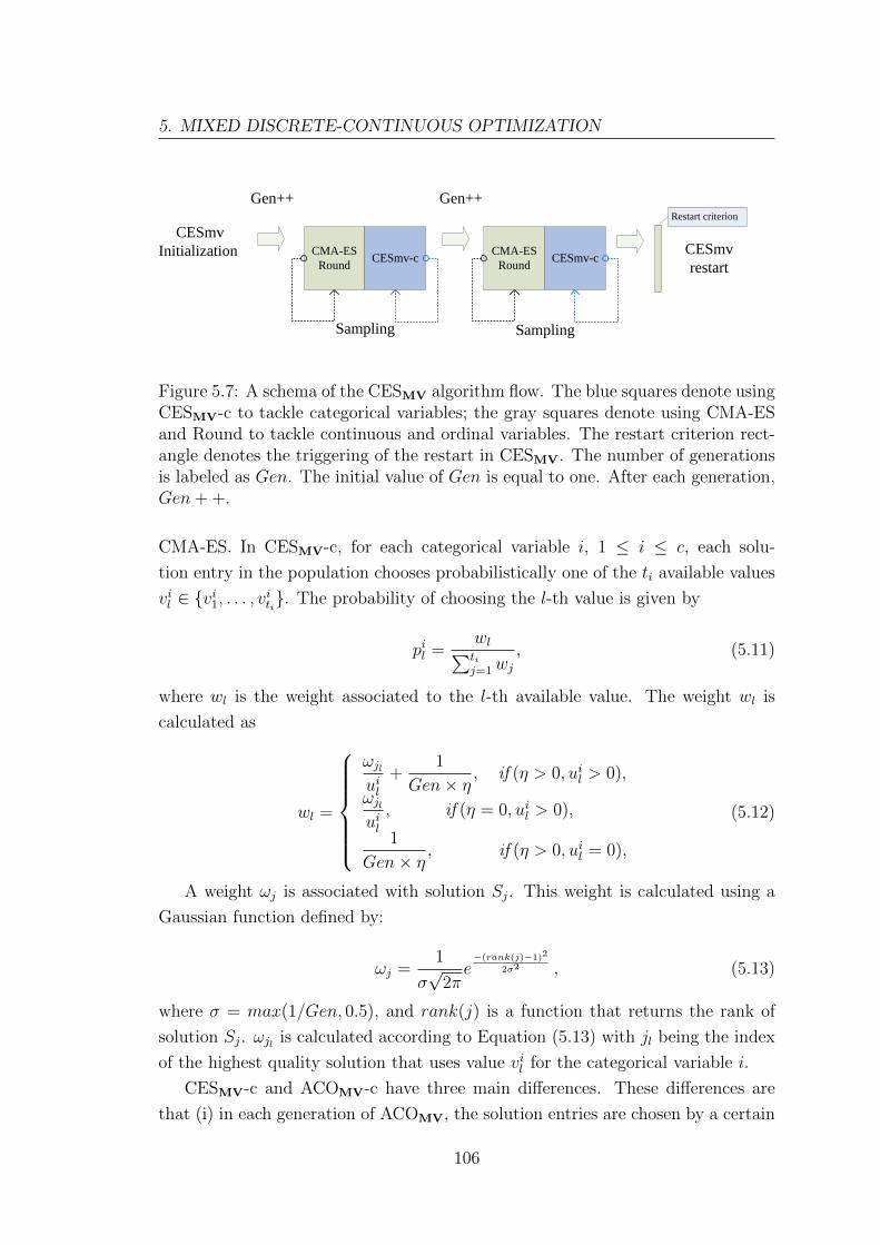
5. MIXED DISCRETE-CONTINUOUS OPTIMIZATION
CMA-ESRound
CESmv-cCMA-ES
RoundCESmv-c
CESmv Initialization
Restart criterion
CESmv restart
Sampling Sampling
Gen++ Gen++
Figure 5.7: A schema of the CESMV algorithm flow. The blue squares denote usingCESMV-c to tackle categorical variables; the gray squares denote using CMA-ESand Round to tackle continuous and ordinal variables. The restart criterion rect-angle denotes the triggering of the restart in CESMV. The number of generationsis labeled as Gen. The initial value of Gen is equal to one. After each generation,Gen+ +.
CMA-ES. In CESMV-c, for each categorical variable i, 1 ≤ i ≤ c, each solu-
tion entry in the population chooses probabilistically one of the ti available values
vil ∈ vi1, . . . , viti. The probability of choosing the l-th value is given by
pil =wl∑tij=1wj
, (5.11)
where wl is the weight associated to the l-th available value. The weight wl is
calculated as
wl =
ωjluil
+1
Gen× η, if (η > 0, uil > 0),
ωjluil, if (η = 0, uil > 0),
1
Gen× η, if (η > 0, uil = 0),
(5.12)
A weight ωj is associated with solution Sj. This weight is calculated using a
Gaussian function defined by:
ωj =1
σ√
2πe−(rank(j)−1)2
2σ2 , (5.13)
where σ = max(1/Gen, 0.5), and rank(j) is a function that returns the rank of
solution Sj. ωjl is calculated according to Equation (5.13) with jl being the index
of the highest quality solution that uses value vil for the categorical variable i.
CESMV-c and ACOMV-c have three main differences. These differences are
that (i) in each generation of ACOMV, the solution entries are chosen by a certain
106

number of ants to sample values, while in each generation of CESMV, each solution
entry in the population is used. (ii) ACOMV-c uses parameter q in Equation 5.8,
while CESMV-c use an adaptive variable 1/Gen to replace with q, resulting the
new Equation 5.12; (iii) The computation of σ in Equation 5.13 does not follow the
way of Equation 5.3. σ in Equation 5.13 is simply defined as σ = max(1/Gen, 0.5).
In CESMV, σ value is therefore kept equal to 0.5 from the second generation on.
This lower bound 0.5 is used to keep CESMV a sufficient deviation to search large
mixed-variable domains.
5.3.3 CES-RelayC
The high performance of CMA-ES in continuous optimization has attracted re-
searchers to extend it to tackle mixed discrete-continuous problems by using a
two-partition strategy [Sambo et al., 2012, Wagner et al., 2011]. The two-partition
strategy for mixed discrete-continuous problems consists in partitioning the vari-
ables into continuous and discrete variables, the variables of one partition are
optimized separately for fixed values of the variables of the other partition. For
instance, in [Wagner et al., 2011], a basic two-partition strategy was successfully
applied for track cycling problem with mixed discrete-continuous variables. CMA-
ES was first used to optimize continuous variables for fixed values of the discrete
variables; then, a simple discrete optimization method (e.g. random search) was
used to optimize discrete variables for setting the continuous variables to the best
found setting in the previous phase.
In this section, we propose CES-RelayC, a relay version following the two-
partition strategy where variables of one partition (containing the categorical ones)
are optimized for fixed values of the variables of the other partition (containing
the continuous and ordinal ones). In CES-RelayC, CESMV-c handles categorical
variables in one partition and IPOP-CMA-ES and Round handle continuous and
ordinal variables in another partition.
We describe CES-RelayC by focusing on how it handles continuous and cat-
egorical variables. The population is initialized with Cpop randomly generated
solutions. CESMV-c is then applied to update the values of the categorical vari-
ables of the Cpop solutions. Next, the best ranked solution of this generation,
SC−Gen, is recorded, and the values of the continuous variables of SC−Gen are used
as the initial solution for IPOP-CMA-ES approach. The values of the categori-
cal variables in SC−Gen remain fixed, while IPOP-CMA-ES is run for a maximum
of Reval function evaluations. Next, the best-so-far solution after running IPOP-
107

5. MIXED DISCRETE-CONTINUOUS OPTIMIZATION
CES-RelayCInitialization CESmv-c
IPOP-CMA-ES and Round (fixed C variables)
CESmv-c
Restart criterion
CES-RelayC restart
Gen++ Gen++
GenCS GenCS
bestROS bestROS
IPOP-CMA-ES and Round (fixed C variables)
Figure 5.8: A schema of the CES-RelayC algorithm flow. After initialization,CESMV-c is first applied to update the values of the categorical variables. Next,the best ranked solution of this phase, SC−Gen, is recorded, and the values of thecontinuous (and ordinal) variables of SC−Gen are used as initial solution for theIPOP-CMA-ES (and Round) phase. Using the values of the categorical variablesfixed to those in SC−Gen, IPOP-CMA-ES (and Round) is then applied, resultingSRO−best. In the next generation, CESMV-c updates the values of the categor-ical variables with those of continuous (and ordinal) variables fixed to those ofin SRO−best. The process continues until the stopping condition CES-RelayC issatisfied. CES-RelayC uses the same restart mechanism as ACOMV for fightingstagnation.
CMA-ES is recorded in SRO−best. With the values of the continuous variables fixed
to those of SRO−best, CESMV-c generates new values of the categorical variables
for the next generation. The process continues until the stopping condition CES-
RelayC is satisfied. CES-RelayC uses the same restart mechanism as ACOMV for
fighting stagnation. A schema of the CES-RelayC algorithm flow is shown in Fig
5.8.
5.4 Automatic tuning and performance evaluation
5.4.1 Automatic tuning
Besides serving for experimental studies, the new benchmark functions proposed
in Section 5.1 can be used to generate a training set of problems for the automatic
parameter tuning of mixed-variable optimization algorithms. The tuning of an
108

Table 5.3: Parameter settings for ACOMV tuned by Iterated F-raceParameter Symbol ValueNumber of ants m 5Influence of best quality solutions q 0.05099Width of the search ξ 0.6795Archive size k 90Stagnating iterations before restart MaxStagIter 650Relative improvement threshold ε 10−5
Table 5.4: Parameter settings for CES-RoundC, CESMV and CES-RelayCParameter Internal parameter CES-RoundC CESMV CES-RelayCa Init pop size: λ0 = 4 + ba ln(D)c 5.679 3.158 5.979b Parent size: µ = bλ/bc 2.216 1.804 1.615c Init step size: σ0 = c · (B −A) 0.23690 0.1597 0.28280d IPOP factor: ipop = d 1.728 1.913 2.722e stopTolFun = 10e −14.62 −10.21 −13.28f stopTolFunHist = 10f −10.14 −12.51 −14.58g stopTolX = 10g −10.21 −11.9 −11.66Cpop Pop size for CESMV-c = Cpop - - 806Reval Evaluations for IPOP-CMA-ES = Reval - - 6078MaxStagIter Stagnating iterations before restart = MaxStagIter - - 20ε Relative improvement threshold = ε - - 10−5
algorithm on a training set that is different from the test set is important to allow
for an unbiased assessment of the algorithm’s performance on (by the algorithm
unseen) test problems [Birattari, 2009]. We therefore generate a training set of
benchmark functions across all six mixed-variable benchmark functions, across
various dimensions [Liao et al., 2011c] (taken from the set n ∈2, 4, 6, 8, 10,
12, 14), and across various ratios of ordinal and categorical variables. As in the
other tuning tasks in this thesis, we use Iterated F-Race [Balaprakash et al., 2007,
Birattari et al., 2010] that is included in the irace [Lopez-Ibanez et al., 2011]. The
performance measure for tuning is the objective function value of each problem
instance after 10 000 function evaluations. The tuning budget for Iterated F-Race
is set to 5 000 runs of each algorithm. We use the default settings of Iterated
F-Race [Birattari et al., 2010, Lopez-Ibanez et al., 2011]. The obtained parameter
settings after tuning ACOMV, CES-RoundC, CESMV, and CES-RelayC are given
in Tables 5.3 and 5.4. Next, we use these parameter settings for a validation of
performance.
5.4.2 Performance evaluation on benchmark functions
First we examine the performance of the three CMA-ES extensions, CES-
RoundC, CESMV and CES-RelayC on artificial mixed-variable benchmark func-
tions (fSphereMV, fEllipsoidMV
, fRosenbrockMV, fAckleyMV
, fRastriginMVand fGriewankMV
)
109

5. MIXED DISCRETE-CONTINUOUS OPTIMIZATION
with continuous and categorical variables and with dimensions four, ten and
twenty. Half of the dimensions are categorical variables and the other half are con-
tinuous variables. The experimental results are measured across 50 independent
runs of 1 000 000 objective function evaluations for instances with t = 10 discrete
points. In Fig. 5.9 we show their run-time behavior by using run-length distribu-
tions (RLDs, for short) [Hoos and Stutzle, 2005]. An (empirical) RLD provides a
graphical view of the development of the empirical frequency of finding a solution
of a certain quality as a function of the number of objective function evaluations.
Except the 10 and 20 dimensional versions of fEllipsoidMVand fRastriginMV
, the so-
lution quality required is set to 1.00E−10, which is used as zero threshold. The
solution quality required for the 10 and 20 dimensional fEllipsoidMVand fRastriginMV
functions is enlarged due to the inherent difficulty of these problems, the required
values are shown in the title of the corresponding RLDs plot. Success rate is the
proportion of successful runs in the total number of runs. A successful run is a run
during which the algorithm finds the required solution quality. Convergence speed
refers to the number of function evaluations used to reach 100% success rate or
a specific success rate required in some cases. Faster (slower) convergence speed
corresponds to fewer (more) function evaluations needed.
CESMV and CES-RoundC
CESMV performs clearly better than CES-RoundC on both success rates and con-
vergence speed. As seen from the simplest fSphereMV, in four, ten and twenty
dimensions CESMV reaches a solution whose objective function value is equal to
or less than 1.00E−10 with probability 1; CES-RoundC reaches a solution whose
objective function value is equal to or less than 1.00E−10 with probability 1, 0.64
and about 0.44 respectively. Comparing to CESMV, CES-RoundC stagnates at
much lower success rates in higher dimensions, and converges much more slowly.
CESMV and CES-RelayC
The success rates reached by CES-RelayC are never lower than 60%. CES-RelayC
reaches a 100% success rate in fSphereMV, fAckleyMV
in all dimensions; in dimen-
sion four, CES-RelayC reaches a 100% success rate for all functions except for
fEllipsoidMV(96%), fRastriginMV
(98%) and fGriewankMV(98%). Only in some cases
such as the ten and twenty dimensional fRosenbrockMVfunction, CES-RelayC stag-
nates at a success rates lower than 100%. CES-RelayC clearly improves over CES-
RoundC. However, CES-RelayC performs worse than CESMV, especially concern-
110

Table 5.5: The number of function evaluations used by CES-RelayC and CESMV
for obtaining a 100% success rate in fSphereMV, fAckleyMV
of each dimension.Function Dimension CES-RelayC CESMV
fSphereMV
4 14 628 2 65710 100 356 7 45120 167 752 15 386
fAckleyMV
4 17 864 5 53610 112 574 15 25720 308 256 37 120
ing convergence speed. CES-RelayC uses much larger number of function evalu-
ations to find the solution quality required than CESMV does. This conclusion
is clearly illustrated by their performance on fSphereMVand fAckleyMV
. Table 5.5
shows the number of function evaluations used by CES-RelayC and CESMV for
obtaining a 100% success rate in fSphereMV, fAckleyMV
of each dimension. Despite
the relay and restart mechanisms in CES-RelayC facilitates the high success rates,
this two partition mechanism converges slower than the CESMV algorithm can
not be avoided. In summary, we identify CESMV as the best performing variant
among the three CMA-ES extensions.
CESMV and ACOMV
Next, we compare the performance of CESMV and ACOMV. As seen from Fig.
5.9, either ACOMV or CESMV obtains the best performance on most of the func-
tions. With respect to success rates, CESMV performs better than ACOMV. Over
dimension four, ten and twenty, CESMV obtains 100% success rate when applied
to solve almost all the functions, while ACOMV stagnates at lower success rates in
some cases such as fRosenbrockMVand fGriewankMV
functions. For fRosenbrockMVand
fGriewankMV, CESMV clearly obtains larger success rates than ACOMV. With re-
spect to convergence speed, in some functions such as fSphereMV, fAckleyMV
, ACOMV
reach 100% success rate faster than CESMV.
We also evaluate the performance of CESMV and ACOMV on the artificial
mixed-variable benchmark functions with continuous and ordinal variables. The
experimental setups are the same as those with categorical variables. As seen from
Fig. 5.10, CESMV and ACOMV reach very similar performance in the benchmark
function with four dimension. In fact, ACOMV even more often reaches 100%
success rate faster than CESMV. However, in dimensions ten and twenty, CESMV
clearly performs better than ACOMV in most cases. Most striking are the example
of the 20 dimensional fRastriginMVand fGriewankMV
functions, for which ACOMV
can not find an optimum solution while CESMV reaches very high success rates.
111

5. MIXED DISCRETE-CONTINUOUS OPTIMIZATION2
contin
uou
san
d2
categoricalvariab
les
Sp
he
re−
ca
teg
oric
al v
aria
ble
s
Nu
mb
er o
f fun
ctio
n e
valu
atio
ns
Probability of solving the problem
10
21
03
10
41
05
10
6
0.0 0.2 0.4 0.6 0.8 1.0
AC
Om
v
CE
S−
Ro
un
dC
CE
Sm
v
CE
S−
Re
layC
Ellip
so
id−
ca
teg
oric
al v
aria
ble
s
Nu
mb
er o
f fun
ctio
n e
valu
atio
ns
Probability of solving the problem
10
21
03
10
41
05
10
6
0.0 0.2 0.4 0.6 0.8 1.0
AC
Om
v
CE
S−
Ro
un
dC
CE
Sm
v
CE
S−
Re
layC
Ro
se
nb
rock
− c
ate
go
rica
l va
riab
les
Nu
mb
er o
f fun
ctio
n e
valu
atio
ns
Probability of solving the problem
10
21
03
10
41
05
10
6
0.0 0.2 0.4 0.6 0.8 1.0
AC
Om
v
CE
S−
Ro
un
dC
CE
Sm
v
CE
S−
Re
layC
Ack
ley
− c
ate
go
rica
l va
riab
les
Nu
mb
er o
f fun
ctio
n e
valu
atio
ns
Probability of solving the problem
10
21
03
10
41
05
10
6
0.0 0.2 0.4 0.6 0.8 1.0
AC
Om
v
CE
S−
Ro
un
dC
CE
Sm
v
CE
S−
Re
layC
Ra
strig
in−
ca
teg
oric
al v
aria
ble
s
Nu
mb
er o
f fun
ctio
n e
valu
atio
ns
Probability of solving the problem
10
21
03
10
41
05
10
6
0.0 0.2 0.4 0.6 0.8 1.0
AC
Om
v
CE
S−
Ro
un
dC
CE
Sm
v
CE
S−
Re
layC
Grie
wa
nk
− c
ate
go
rica
l va
riab
les
Nu
mb
er o
f fun
ctio
n e
valu
atio
ns
Probability of solving the problem
10
21
03
10
41
05
10
6
0.0 0.2 0.4 0.6 0.8 1.0
AC
Om
v
CE
S−
Ro
un
dC
CE
Sm
v
CE
S−
Re
layC
5con
tinu
ous
and
5categorical
variables
Sp
he
re−
ca
teg
oric
al v
aria
ble
s
Nu
mb
er o
f fun
ctio
n e
valu
atio
ns
Probability of solving the problem
10
21
03
10
41
05
10
6
0.0 0.2 0.4 0.6 0.8 1.0
AC
Om
v
CE
S−
Ro
un
dC
CE
Sm
v
CE
S−
Re
layC
Ellip
so
id−
ca
teg
oric
al v
aria
ble
s−
(1e
+2
)
Nu
mb
er o
f fun
ctio
n e
valu
atio
ns
Probability of solving the problem
10
21
03
10
41
05
10
6
0.0 0.2 0.4 0.6 0.8 1.0A
CO
mv
CE
S−
Ro
un
dC
CE
Sm
v
CE
S−
Re
layC
Ro
se
nb
rock
− c
ate
go
rica
l va
riab
les
Nu
mb
er o
f fun
ctio
n e
valu
atio
ns
Probability of solving the problem
10
21
03
10
41
05
10
6
0.0 0.2 0.4 0.6 0.8 1.0
AC
Om
v
CE
S−
Ro
un
dC
CE
Sm
v
CE
S−
Re
layC
Ack
ley
− c
ate
go
rica
l va
riab
les
Nu
mb
er o
f fun
ctio
n e
valu
atio
ns
Probability of solving the problem
10
21
03
10
41
05
10
6
0.0 0.2 0.4 0.6 0.8 1.0
AC
Om
v
CE
S−
Ro
un
dC
CE
Sm
v
CE
S−
Re
layC
Ra
strig
in−
ca
teg
oric
al v
aria
ble
s (2
e+
1)
Nu
mb
er o
f fun
ctio
n e
valu
atio
ns
Probability of solving the problem
10
21
03
10
41
05
10
6
0.0 0.2 0.4 0.6 0.8 1.0
AC
Om
v
CE
S−
Ro
un
dC
CE
Sm
v
CE
S−
Re
layC
Grie
wa
nk
− c
ate
go
rica
l va
riab
les
Nu
mb
er o
f fun
ctio
n e
valu
atio
ns
Probability of solving the problem
10
21
03
10
41
05
10
6
0.0 0.2 0.4 0.6 0.8 1.0
AC
Om
v
CE
S−
Ro
un
dC
CE
Sm
v
CE
S−
Re
layC
10con
tinu
ous
and
10categorical
variables
Sp
he
re−
ca
teg
oric
al v
aria
ble
s
Nu
mb
er o
f fun
ctio
n e
valu
atio
ns
Probability of solving the problem
10
21
03
10
41
05
10
6
0.0 0.2 0.4 0.6 0.8 1.0
AC
Om
v
CE
S−
Ro
un
dC
CE
Sm
v
CE
S−
Re
layC
Ellip
so
id−
ca
teg
oric
al v
aria
ble
s−
(1e
+3
)
Nu
mb
er o
f fun
ctio
n e
valu
atio
ns
Probability of solving the problem
10
21
03
10
41
05
10
6
0.0 0.2 0.4 0.6 0.8 1.0
AC
Om
v
CE
S−
Ro
un
dC
CE
Sm
v
CE
S−
Re
layC
Ro
se
nb
rock
− c
ate
go
rica
l va
riab
les
Nu
mb
er o
f fun
ctio
n e
valu
atio
ns
Probability of solving the problem
10
21
03
10
41
05
10
6
0.0 0.2 0.4 0.6 0.8 1.0
AC
Om
v
CE
S−
Ro
un
dC
CE
Sm
v
CE
S−
Re
layC
Ack
ley
− c
ate
go
rica
l va
riab
les
Nu
mb
er o
f fun
ctio
n e
valu
atio
ns
Probability of solving the problem
10
21
03
10
41
05
10
6
0.0 0.2 0.4 0.6 0.8 1.0
AC
Om
v
CE
S−
Ro
un
dC
CE
Sm
v
CE
S−
Re
layC
Ra
strig
in−
ca
teg
oric
al v
aria
ble
s−
(2e
+2
)
Nu
mb
er o
f fun
ctio
n e
valu
atio
ns
Probability of solving the problem
10
11
02
10
31
04
0.0 0.2 0.4 0.6 0.8 1.0
AC
Om
v
CE
S−
Ro
un
dC
CE
Sm
v
CE
S−
Re
layC
Grie
wa
nk
− c
ate
go
rica
l va
riab
les
Nu
mb
er o
f fun
ctio
n e
valu
atio
ns
Probability of solving the problem
10
21
03
10
41
05
10
6
0.0 0.2 0.4 0.6 0.8 1.0
AC
Om
v
CE
S−
Ro
un
dC
CE
Sm
v
CE
S−
Re
layC
Figu
re5.9:
The
qualifi
edru
n-len
gthdistrib
ution
s(R
LD
s,for
short)
over50
indep
enden
tru
ns
obtain
edby
AC
OM
V,
CE
S-
Rou
ndC
,C
ESM
Van
dC
ES-R
elayC
.T
he
solution
quality
required
is1.00E−
10(zero
thresh
old)
excep
tfor
the
10an
d20
dim
ension
alfEllip
soidMV
andfRastriginMV
,for
which
the
solution
quality
required
issh
own
inth
etitle
ofth
ecorresp
ondin
gplot.
112

2co
nti
nu
ous
and
2or
din
alva
riab
les
Sp
he
re−
ord
ina
l va
ria
ble
s
Nu
mb
er
of
fun
ctio
n e
valu
atio
ns
Probability of solving the problem
10
21
03
10
41
05
10
6
0.00.20.40.60.81.0
AC
Om
v
CE
Sm
v
Ell
ips
oid
− o
rdin
al
va
ria
ble
s
Nu
mb
er
of
fun
ctio
n e
valu
atio
ns
Probability of solving the problem 1
02
10
31
04
10
51
06
0.00.20.40.60.81.0
AC
Om
v
CE
Sm
v
Ro
se
nb
rock
− o
rdin
al
va
ria
ble
s
Nu
mb
er
of
fun
ctio
n e
valu
atio
ns
Probability of solving the problem
10
21
03
10
41
05
10
6
0.00.20.40.60.81.0
AC
Om
v
CE
Sm
v
Ack
ley
− o
rdin
al
va
ria
ble
s
Nu
mb
er
of
fun
ctio
n e
valu
atio
ns
Probability of solving the problem
10
21
03
10
41
05
10
6
0.00.20.40.60.81.0
AC
Om
v
CE
Sm
v
Ra
str
igin
− o
rdin
al
va
ria
ble
s
Nu
mb
er
of
fun
ctio
n e
valu
atio
ns
Probability of solving the problem
10
21
03
10
41
05
10
6
0.00.20.40.60.81.0
AC
Om
v
CE
Sm
v
Grie
wa
nk
− o
rdin
al
va
ria
ble
s
Nu
mb
er
of
fun
ctio
n e
valu
atio
ns
Probability of solving the problem
10
21
03
10
41
05
10
6
0.00.20.40.60.81.0
AC
Om
v
CE
Sm
v
5co
nti
nu
ous
and
5or
din
alva
riab
les
Sp
he
re−
ord
ina
l va
ria
ble
s
Nu
mb
er
of
fun
ctio
n e
valu
atio
ns
Probability of solving the problem
10
21
03
10
41
05
10
6
0.00.20.40.60.81.0
AC
Om
v
CE
Sm
v
Ell
ips
oid
− o
rdin
al
va
ria
ble
s
Nu
mb
er
of
fun
ctio
n e
valu
atio
ns
Probability of solving the problem
10
21
03
10
41
05
10
6
0.00.20.40.60.81.0
AC
Om
v
CE
Sm
v
Ro
se
nb
rock
− o
rdin
al
va
ria
ble
s
Nu
mb
er
of
fun
ctio
n e
valu
atio
ns
Probability of solving the problem 1
02
10
31
04
10
51
06
0.00.20.40.60.81.0
AC
Om
v
CE
Sm
v
Ack
ley
− o
rdin
al
va
ria
ble
s
Nu
mb
er
of
fun
ctio
n e
valu
atio
ns
Probability of solving the problem
10
21
03
10
41
05
10
6
0.00.20.40.60.81.0
AC
Om
v
CE
Sm
v
Ra
str
igin
− o
rdin
al
va
ria
ble
s
Nu
mb
er
of
fun
ctio
n e
valu
atio
ns
Probability of solving the problem
10
21
03
10
41
05
10
6
0.00.20.40.60.81.0
AC
Om
v
CE
Sm
v
Grie
wa
nk
− o
rdin
al
va
ria
ble
s
Nu
mb
er
of
fun
ctio
n e
valu
atio
ns
Probability of solving the problem
10
21
03
10
41
05
10
6
0.00.20.40.60.81.0
AC
Om
v
CE
Sm
v
10co
nti
nu
ous
and
10or
din
alva
riab
les
Sp
he
re−
ord
ina
l va
ria
ble
s
Nu
mb
er
of
fun
ctio
n e
valu
atio
ns
Probability of solving the problem
10
21
03
10
41
05
10
6
0.00.20.40.60.81.0
AC
Om
v
CE
Sm
v
Ell
ips
oid
− o
rdin
al
va
ria
ble
s−
(1
e+
3)
Nu
mb
er
of
fun
ctio
n e
valu
atio
ns
Probability of solving the problem
10
21
03
10
41
05
10
6
0.00.20.40.60.81.0
AC
Om
v
CE
Sm
v
Ro
se
nb
rock
− o
rdin
al
va
ria
ble
s
Nu
mb
er
of
fun
ctio
n e
valu
atio
ns
Probability of solving the problem
10
21
03
10
41
05
10
6
0.00.20.40.60.81.0
AC
Om
v
CE
Sm
v
Ack
ley
− o
rdin
al
va
ria
ble
s
Nu
mb
er
of
fun
ctio
n e
valu
atio
ns
Probability of solving the problem
10
21
03
10
41
05
10
6
0.00.20.40.60.81.0
AC
Om
v
CE
Sm
v
Ra
str
igin
− o
rdin
al
va
ria
ble
s
Nu
mb
er
of
fun
ctio
n e
valu
atio
ns
Probability of solving the problem
10
21
03
10
41
05
10
6
0.00.20.40.60.81.0
AC
Om
v
CE
Sm
v
Grie
wa
nk
− o
rdin
al
va
ria
ble
s
Nu
mb
er
of
fun
ctio
n e
valu
atio
ns
Probability of solving the problem
10
21
03
10
41
05
10
6
0.00.20.40.60.81.0
AC
Om
v
CE
Sm
v
Fig
ure
5.10
:T
he
qual
ified
run-l
engt
hdis
trib
uti
ons
(RL
Ds,
for
shor
t)ov
er50
indep
enden
tru
ns
obta
ined
by
AC
OM
Van
dC
ESM
V.
The
solu
tion
qual
ity
requir
edis
1.00
E−
10(z
ero
thre
shol
d)
exce
pt
for
the
20dim
ensi
onalf E
llipsoidMV
for
whic
hth
eso
luti
onqual
ity
requir
edis
show
nin
the
titl
eof
the
corr
esp
ondin
gplo
t.
113

5. MIXED DISCRETE-CONTINUOUS OPTIMIZATION
5.5 Application to engineering optimization problems
In this section, we apply ACOMV and CESMV into mixed discrete-continuous
engineering benchmark problems and compare the results of ACOMV and CESMV
with those found in the literature. Note that our experiments comprise a larger
set of benchmark problems than in any of the papers found in the literature, since
these papers are often limited to a specific type of discrete variables (either ordinal
or categorical). First, we classify the available engineering optimization problems
in the literature into four groups according to the types of the decision variables
used (see Table 5.6).
Table 5.6: The classification of engineering optimizationproblems.
Groups The type of decision variablesGroup I Continuous variables†
Group II Continuous and ordinal variablesGroup III Continuous and categorical variablesGroup IV Continuous, ordinal and categorical variables† Problems with only continuous variables are considered
as a particular class of mixed variables with an empty setof discrete variables, since ACOMV and CESMV are alsocapable to solve pure continuous optimization problems.
Group I includes the welded beam design problem case A [Coello Coello, 2000];
Group II the pressure vessel design problem [Sandgren, 1990] and the coil spring
design problem [Sandgren, 1990]; Group III the thermal insulation systems design
problem [Kokkolaras et al., 2001]; and Group IV the welded beam design problem
case B [Deb and Goyal, 1996]. The mathematical formulations of the problems are
given in Appendix B. In this section, we compare the results obtained by ACOMV
and CESMV to those reported in the literature for these problems. We also show
the run-time behavior of ACOMV and CESMV by using RLDs. It is important
to note that NM-PSO [Zahara and Kao, 2009] and PSOLVER [Kayhan et al.,
2010] report infeasible solutions that violate the problems’ constraints; Crepinsek
et al. [Crepinsek et al., 2012] pointed out that the authors of TLBO [Rao et al.,
2011] used an incorrect formula for computing the number of objective function
evaluations. Therefore, we did not include these three algorithms in our compar-
ison. For our experiments, the tuned parameter configurations from Tables 5.3
and 5.4 were used. For simplifying the algorithm and giving prominence to the
role of the ACOMV and CESMV heuristic itself, the most fundamental constraint
114

handling technique was used, which consists in rejecting all infeasible solutions in
the optimization process (also called “death penalty”). 100 independent runs were
performed for each engineering problem. In the comparisons, fBest, fMean and
fWorst are the abbreviations used to indicate the best, average and worst objective
function values obtained, respectively. SRB denotes the success rate of reaching
the best known solution value. Sd gives the standard deviation of the mean objec-
tive function value; a value of Sd lower than 1.00E−10 is reported as 0. FEs gives
the maximum number of objective function evaluations in each algorithm run.
Note that the value of FEs may vary from algorithm to algorithm. To define the
value of FEs for ACOMV and CESMV, we first checked which is the smallest value
of FEs used across all competing algorithms; let this value be denoted by FEsmin.
Then the value of FEs for ACOMV and CESMV is set to FEsmin. Often, however,
ACOMV and CESMV reached the best known solution values for the particular
problem under concern in all runs (that is, with a 100% success rate) much faster
than its competitors. In such cases, for ACOMV and CESMV we give, instead
of the value FEsmin, in parenthesis the maximum number of objective function
evaluations we observed across the 100 independent runs.
Group I : Welded beam design problem case A
Recently, many methods have been applied to the welded beam design problem
case A. Table 5.7 shows basic summary statistics of the results obtained by nine
other algorithms, ACOMV and CESMV. Most other algorithms do not reach a
success rate of 100% within a maximum number of objective function evaluations
ranging from 30 000 (for (µ + λ)ES [Mezura Montes and Coello Coello, 2005]) to
200 000 (for CPSO [He and Wang, 2007a]), while ACOMV and CESMV find the
best-known solution value in every run using at most 2 303 and 2 070 objective
function evaluations (measured across 100 independent trials). The only other
algorithm that reaches the best-known solution value in every run is DELC [Wang
and Li, 2010]; it does so using in every run at most 20 000 objective function
evaluations (measured across 30 independent trials). Hence, ACOMV and CESMV
are very efficient and robust algorithms for this problem. The run-time behavior
of ACOMV and CESMV on this problems is illustrated also in Fig. 5.11, where the
RLDs for this problem are given. The average and minimum number of objective
function evaluations for ACOMV are 2 122 and 1 888, respectively. The average
and minimum number of objective function evaluations for CESMV are 1 550 and
1 173, respectively.
115

5. MIXED DISCRETE-CONTINUOUS OPTIMIZATION
1000 1500 2000 2500 3000
0.0
0.2
0.4
0.6
0.8
1.0
wbdA
Function evaluations
Pro
ba
bili
ty o
f so
lvin
g t
he
pro
ble
m
0.0
0.2
0.4
0.6
0.8
1.0
ACOmv
CESmv
pvdA
Function evaluations
Pro
ba
bili
ty o
f so
lvin
g t
he
pro
ble
m
103
1040
.00
.20
.40
.60
.81
.0
ACOmv
CESmv
pvdB
Function evaluations
Pro
ba
bili
ty o
f so
lvin
g t
he
pro
ble
m
103
1040
.00
.20
.40
.60
.81
.0
ACOmv
CESmv
pvdC
Function evaluations
Pro
ba
bili
ty o
f so
lvin
g t
he
pro
ble
m
103
1040
.00
.20
.40
.60
.81
.0
ACOmv
CESmv
Figure 5.11: The RLDs of ACOMV and CESMV for the welded beam design prob-lem case A and the pressure vessel design problem case A, B and C (wbdA, pvdA,pvdB and pvdC are the abbreviations of those problems, respectively).
116

Table 5.7: Basic summary statistics for the welded beam design problem case A.The best-known solution value is 1.724852. fBest, fMean and fWorst denote the best,mean and worst objective function values, respectively. Sd denotes the standarddeviation of the mean objective function value. FEs denotes the maximum numberof objective function evaluations in each algorithm run. For ACOMV and CESMV
we report in parenthesis the largest number of objective function evaluations itrequired in any of the 100 independent runs (ACOMV and CESMV reached ineach run of at most 20 000 evaluations the best known solution value). “-” meansthat the information is not available.
Methods fBest fMean fWorst Sd FEsGA1 [Coello Coello, 2000] 1.748309 1.771973 1.785835 1.12E−02 -GA2 [Coello Coello and Mezura Montes, 2002] 1.728226 1.792654 1.993408 7.47E−02 80 000EP [Coello Coello and Becerra, 2004] 1.724852 1.971809 3.179709 4.43E−01 -(µ+ λ)ES [Mezura Montes and Coello Coello, 2005] 1.724852 1.777692 - 8.80E−02 30 000CPSO [He and Wang, 2007a] 1.728024 1.748831 1.782143 1.29E−02 200 000HPSO [He and Wang, 2007b] 1.724852 1.749040 1.814295 4.01E−02 81 000CLPSO [Gao and Hailu, 2010] 1.724852 1.728180 - 5.32E−03 60 000DELC [Wang and Li, 2010] 1.724852 1.724852 1.724852 0 20 000ABC [Akay and Karaboga] 1.724852 1.741913 - 3.10E−02 30 000ACOMV 1.724852 1.724852 1.724852 0 (2 303)CESMV 1.724852 1.724852 1.724852 0 (2 070)
Group II: Pressure vessel design problem case A, B, C and D
There are four distinct cases (A, B, C and D) of the pressure vessel design problem
defined in the literature. These cases differ by the constraints posed on the thick-
ness of the steel used for the heads and the main cylinder. In case A, B and C (see
Table 5.8), ACOMV reaches the best-known solution value with a 100% success
rate in a maximum of 1 737, 1 764 and 1 666 objective function evaluations, respec-
tively; the average number of objective function evaluations of the successful runs
are 1 500, 1 470 and 1 433 respectively. CESMV reaches the best-known solution
value with a 100% success rate in a maximum of 5 021, 4 612 and 4 568 objec-
tive function evaluations, respectively; the average number of objective function
evaluations of the successful runs are 1 381, 1 313 and 1 604 respectively. Other
algorithms do not reach a success rate of 100% with respect to the best-known
solution value even after many more objective function evaluations. The run-time
behavior of ACOMV and CESMV is illustrated in Fig. 5.11, where the RLDs for
these problems are given.
Case D is more difficult to solve due to the larger range of side constraints for
decision variables. Therefore, Case D was analyzed in more detail in the recent
literature. We limit ACOMV and CESMV to use a maximum number of 30 000
objective function evaluations, the same as done for several other approaches from
117

5. MIXED DISCRETE-CONTINUOUS OPTIMIZATION
Tab
le5.8:
Resu
ltsfor
caseA
,B
and
Cof
the
pressu
revessel
design
prob
lem.fBest
den
otesth
eb
estob
jectivefu
nction
value.
SRB
den
otesth
esu
ccessrate
ofreach
ing
the
best
know
nsolu
tionvalu
e.F
Es
den
otesth
em
axim
um
num
ber
ofob
jectivefu
nction
evaluation
sin
eachalgorith
mru
n.
For
AC
OM
Van
dC
ESM
Vw
erep
ortin
paren
thesis
the
largestnum
ber
ofob
jectivefu
nction
evaluation
sit
required
inan
yof
the
100in
dep
enden
tru
ns
(AC
OM
Van
dC
ESM
Vreach
edin
eachru
nth
eb
estknow
nsolu
tionvalu
e).G
ivenis
alsoth
eaverage
num
ber
ofob
jectivefu
nction
evaluation
sof
the
successfu
lru
ns.
“-”m
eans
that
the
inform
ationis
not
available.
Case
AN
LID
PM
IDC
PD
EA
CO
MV
CE
SM
V[S
an
dgren
,1990]
[Fu
etal.,
1991]
[Lam
pin
enan
dZ
elinka,
1999c]
fBest
7867.0
7790.5
88
7019.0
31
7019.0
31
7019.0
31
SRB
--
89.2
%100%
100%
FE
s-
-10
000
(1737)
(150
0.0)(5
021)
(1380.86
)
Case
BN
LID
PS
LA
GA
DE
HS
IAA
CO
MV
CE
SM
V[S
an
dgren
,1990]
[Loh
an
dP
ap
ala
mb
ros,
1991]
[Wu
an
dC
how
,1995]
[Lam
pin
enan
dZ
elinka,
1999c]
[Gu
oet
al.,
2004]
fBest
7982.5
7197.7
34
7207.4
97
7197.7
29
7197.9
7197.7
29
7197.7
29
SRB
--
-90.2
%-
100%
100%
FE
s-
--
10
000
-(1
764)
(1470
.48)
(4612)
(1313.34
)
Case
CN
LM
DP
EP
ES
DE
CH
OP
AA
CO
MV
CE
SM
V[L
ian
dC
hou
,1994]
[Cao
an
dW
u,
1997]
[Th
ierau
fan
dC
ai,
2000]
[Lam
pin
enan
dZ
elinka,
1999c]
[Sch
mid
tan
dT
hiera
uf,
2005]
fBest
7127.3
7108.6
16
7006.9
7006.3
58
7006.5
17
006.3
58
7006.3
58
SRB
--
-98.3
%-
100%
100%
FE
s-
-4
800
10
000
10
000
(1666)
(1433
.42)
(4568)
(1603.73
)
118

Table 5.9: Basic summary statistics for the pressure vessel design problem caseD. The best-known objective function value is 6059.7143. fBest, fMean and fWorst
denotes the best, mean and worst objective function values, respectively. Sd de-notes the standard deviation of the mean objective function value. FEs denotesthe maximum number of objective function evaluations in each algorithm run.“-”means that the information is not available.
Methods fBest fMean fWorst Sd FEsGA1 [Coello Coello, 2000] 6 288.7445 6 293.8432 6 308.1497 7.413E+00 -GA2 [Coello Coello and Mezura Montes, 2002] 6 059.9463 6 177.2533 6 469.3220 1.309E+02 80 000(µ+ λ)ES [Mezura Montes and Coello Coello, 2005] 6 059.7143 6 379.9380 - 2.10E+02 30 000CPSO [He and Wang, 2007a] 6 061.0777 6 147.1332 6 363.8041 8.645E+01 200 000HPSO [He and Wang, 2007b] 6 059.7143 6 099.9323 6 288.6770 8.620E+01 81 000RSPSO [Wang and Yin, 2008] 6 059.7143 6 066.2032 6 100.3196 1.33E+01 30 000CLPSO [Gao and Hailu, 2010] 6 059.7143 6 066.0311 - 1.23E+01 60 000DELC [Wang and Li, 2010] 6 059.7143 6 059.7143 6 059.7143 0 30 000ABC [Akay and Karaboga] 6 059.7143 6 245.3081 - 2.05E+02 30 000ACOMV 6 059.7143 6 059.7164 6 059.9143 1.94E−02 30 000CESMV 6 059.7143 6 059.7480 6 089.9893 4.34E+00 30 000
the literature. Table 5.9 shows clearly the second and the third best performing
algorithms for what concerns the average and the worst objective function values.
In fact, ACOMV and CESMV reaches a 100% success rate (measured over 100
independent runs) at 30 717 and 43 739 objective function evaluations, while at
30 000 evaluations they reached a success rate of 98% and 76%, which are slightly
lower than the success rate of 100% reported by DELC [Wang and Li, 2010]. The
run-time behavior of ACOMV and CESMV are illustrated in Fig. 5.12, where the
RLD for this problem is given. The average and minimum number of objective
function evaluations of ACOMV is 9 448 and 1 726, respectively. The average and
minimum number of objective function evaluations of CESMV is 19 675 and 1 417,
respectively.
It is noteworthy that DELC [Wang and Li, 2010] reaches the aforementioned
performance using parameter settings that are specific for each test problem, while
we use a same parameter setting for all test problems. Using instance specific
parameter settings potentially biases the results in favor of the DELC algorithm.
In a practical setting, one would not know a priori which parameter setting to apply
before actually solving the problem. Thus, there are methodological problems in
the results presented for DELC [Wang and Li, 2010].
119

5. MIXED DISCRETE-CONTINUOUS OPTIMIZATION
Group II: Coil spring design problem
Most of the research reported in the literature considering the coil spring design
problem focused on reaching the best-known solution or improving the best-known
one. Only recent work [Datta and Figueira, 2010, Lampinen and Zelinka, 1999c]
gave some attention to the number of objective functions evaluations necessary to
reach the best-known solution. A comparison of the obtained results is presented
in Table 5.10. Only a differential evolution algorithm [Lampinen and Zelinka,
1999c], ACOMV and CESMV obtained the best-known objective function value,
2.65856. At 8 000 evaluations ACOMV and CESMV reached success rates of 74%
and 44%, which are lower than the success rate of 95% reported by the DE al-
gorithm of [Lampinen and Zelinka, 1999c]; however, ACOMV and CESMV reach
100% and 93% success rates with 19 588 and 47 792 objective function evaluations,
respectively. The run-time behavior of ACOMV is illustrated in Fig. 5.12, where
the RLD for this problem is given. The average and minimum number of objective
function evaluations of ACOMV are 9 948 and 1 726, respectively. The average and
minimum number of objective function evaluations of CESMV are 12 107 and 527,
respectively.
It is important to note that the DE algorithm of [Lampinen and Zelinka,
1999c] was not designed to handle categorical variables. Another DE algorithm
proposed in [Datta and Figueira, 2010] did not report a success rate, but the
corresponding objective function values were reported to be in the range of
[2.658565, 2.658790] and the number of objective function evaluations varied in the
range [539 960, 3 711 560], thus, showing a clearly worse performance than ACOMV
and CESMV.
Group III: Thermal insulation systems design problem
The thermal insulation systems design problem is one of the engineering problems
used in the literature that deals with categorical variables. In previous studies,
the categorical variables describing the type of insulators used in different layers
were not considered as optimization variables, but rather as parameters. Only the
more recent work of Kokkolaras et al. [Kokkolaras et al., 2001] and Abramson et
al. [Abramson, 2004], which are able to handle such categorical variables properly,
consider these variables for optimization. Research focuses on improving the best-
known solution value for this difficult engineering problem. ACOMV and CESMV
reaches a better solution than MVP [Kokkolaras et al., 2001] and FMGPS [Abram-
son, 2004]; Table 5.11 presents the best found solutions by the four algorithms we
120

0 10000 30000 50000
0.0
0.2
0.4
0.6
0.8
1.0
pvdD
Function evaluations
Pro
ba
bili
ty o
f so
lvin
g t
he
pro
ble
m
ACOmv
CESmv
csd
Function evaluations
Pro
ba
bili
ty o
f so
lvin
g t
he
pro
ble
m
500 103
104
5 × 1040
.00
.20
.40
.60
.81
.0ACOmv
CESmv
Figure 5.12: The RLDs of ACOMV and CESMV for the pressure vessel design prob-lem case D and the coil spring design problem (pvdD and csd are the abbreviationsof those problems, respectively).
Table 5.10: Results for the coil spring design problem. fBest denotes the best ob-jective function value. SRB denotes the success rate of reaching the best knownsolution value. FEs denotes the maximum number of objective function evalua-tions in each algorithm run. For ACOMV and CESMV we report in parenthesis thelargest number of objective function evaluations it required in any of the 100 inde-pendent runs (ACOMV and CESMV reached in each run the best known solutionvalue). “-” means that the information is not available.
AlgsNLIDP GA GA DE
[Sandgren, 1990] [Chen and Tsao, 1993] [Wu and Chow, 1995] [Lampinen and Zelinka, 1999c]N 10 9 9 9
D [inch] 1.180701 1.2287 1.227411 1.223041d [inch] 0.283 0.283 0.283 0.283fBest 2.7995 2.6709 2.6681 2.65856SRB - - - 95.0%FEs - - - 8 000
AlgsHSIA DE
ACOMV CESMV[Guo et al., 2004] [Datta and Figueira, 2010]N 9 9 9 9
D [inch] 1.223 1.223044 1.223041 1.223041d [inch] 0.283 0.283 0.283 0.283fBest 2.659 2.658565 2.65856 2.65856SRB - - 74% (100%) 44% (93%)FEs - - 8 000 (19 588) 8 000 (47 792)
121

5. MIXED DISCRETE-CONTINUOUS OPTIMIZATION
Table 5.11: Comparison of the best fitness value for the thermal insulation systemsdesign problem
Objective function MVP [Kokkolaras et al., 2001] FMGPS [Abramson, 2004] ACOMV CESMV
Power(PLA
( Wcm
)) 25.294 25.58 24.148 23.914
Function evaluations
Be
st
fitn
ess v
alu
e
0 10000 30000 50000
24
25
26
27
28
29
30
ACOmv
CESmv
Problem Tisdu
Figure 5.13: The best solution trail of ACOMV and CESMV for the thermal insu-lation systems design problem
wbdB
Function evaluations
Pro
ba
bili
ty o
f so
lvin
g t
he
pro
ble
m
600103
104
1050
.00
.20
.40
.60
.81
.0
ACOmv
CESmv
Figure 5.14: The RLDs of ACOMV and CESMV for the welded beam design prob-lem case B (wbdB is its abbreviation).
compare here. Both, ACOMV and CESMV improve over the best solution found
by MVP and FMGPS.
The evolution of the best solution as a function of number of objective function
evaluations of ACOMV and CESMV are shown in Fig.5.13. In fact, as the number of
objective function evaluations increases, the solution quality continues to improve,
though ACOMV appears to show issues of early convergence.
122

Table 5.12: Basic summary statistics for welded beam design design problem caseB. fBest and fMean denotes the best and mean objective function values, respec-tively. Sd denotes the standard deviation of the mean objective function value.Mean-FEs-Success denotes the average number of evaluations of the successfulruns. “-” means that the information is not available.
Methods fBest fMean Sd Mean-FEs-SuccessGeneAS [Deb and Goyal, 1996] 1.9422 - - -RSPSO [Wang and Yin, 2008] 1.9421 - - -PSOA[Dimopoulos, 2007] 1.7631 1.7631 0 6 570CLPSO [Gao and Hailu, 2010] 1.5809 1.7405 2.11E−01 -ACOMV 1.5029 1.5029 0 1 436CESMV 1.5029 1.5029 0 4 188
Group IV: Welded beam design problem case B
The welded beam design problem case B is taken from Deb and Goyal [Deb and
Goyal, 1996] and Dimopoulos [Dimopoulos, 2007]. It is a variation of case A
and it includes ordinal and categorical variables. Table 5.12 shows that ACOMV
and CESMV reaches a new best-known solution value with a 100% success rate.
Additionally, the average number of objective function evaluations required by
ACOMV and CESMV are also fewer than that of PSOA [Dimopoulos, 2007]. The
run-time behavior of ACOMV and CESMV is illustrated in Fig. 5.14.
5.6 Summary
In this chapter, we have presented two algorithms for mixed discrete continuous
optimization problems. One of these algorithms is an ant colony optimization
algorithm, ACOMV, that extends the ACOR method to mixed discrete contin-
uous optimization. In particular, ACOMV integrates a continuous optimization
solver (ACOR), a continuous relaxation approach (ACOMV-o) and a categori-
cal optimization approach (ACOMV-c) to solve continuous and mixed discrete-
continuous optimization problems. As a second algorithm, we have introduced
CESMV, an covariance matrix adaptation evolution strategy algorithm for tack-
ling mixed discrete-continuous optimization problems. CESMV integrates a con-
tinuous optimization solver (CMA-ES), a continuous relaxation approach (Round,
same as ACOMV-o) and a categorical optimization approach (CESMV-c ) to solve
continuous and mixed discrete-continuous optimization problems. The categori-
cal optimization part of CESMV is adapted in a rather straightforward way from
the way ACOMV handles categorical variables. We have also proposed and evalu-
ated other CMA-ES extensions we proposed for tackling mixed discrete-continuous
123

5. MIXED DISCRETE-CONTINUOUS OPTIMIZATION
optimization problems, and identify CESMV as the most performing variant.
We have also proposed a new set of artificial mixed discrete-continuous bench-
mark functions.
We evaluate ACOMV and CESMV on the artificial mixed discrete-continuous
benchmark functions and apply them into real-world engineering problems. The
experimental results for real-world engineering problems illustrate that ACOMV
and CESMV not only can tackle various classes of decision variables robustly, but
also that they are efficient in finding high-quality solutions when compared to
many other algorithms from the literature. In the welded beam design case A,
ACOMV and CESMV are the ones of the three available algorithms that reach
the best-known solution with a 100% success rate; in the pressure vessel design
problem case A, B and C, ACOMV and CESMV are the only two available al-
gorithms that reach the best-known solution with a 100% success rate. In these
four problems, ACOMV and CESMV do so using fewer objective function evalua-
tions than those used by the competing algorithms. In the pressure vessel design
problem case D, ACOMV and CESMV are two of the three available algorithms
that reach the best-known solution with a 100% success rate, and they do so using
only slightly more objective function evaluations than the other algorithm, which
uses problem specific parameter tuning to boost algorithm performance. In the
coil spring design problem, ACOMV is the only available algorithm that reaches
the best-known solution with a 100% success rate. In the thermal insulation sys-
tems design problem, ACOMV and CESMV obtains new best solutions, and in
the welded beam design problem case B, ACOMV and CESMV obtain new best
solutions with a 100% success rate in fewer evaluations than those used by the
other algorithms.
124
Chapter 6
Summary and future work
6.1 Summary
This thesis focuses on the design, engineering and configuration of high-performing
heuristic optimization algorithms for tackling continuous and mixed discrete-
continuous optimization problems. Continuous optimization problems have vari-
able domains that typically are a subset of the real numbers; mixed discrete-
continuous optimization problems have additionally discrete variables, so that
some variables are continuous and others are on an ordinal or categorical scale.
Continuous and mixed discrete-continuous problems have a wide range of appli-
cations in many disciplines and these problems are also often hard to solve due to
their inherent difficulties such as a large number of variables, many local optima
or other factors making problems hard.
We tackle continuous and mixed discrete-continuous optimization problems
with two types of population-based heuristic algorithms, ant colony optimization
(ACO) algorithms and evolution strategies. The main contributions of this thesis
are that (i) we advance the design and engineering of ACO algorithms; the resulting
algorithms are competitive or superior to recent state-of-the-art algorithms for
continuous and mixed discrete-continuous optimization problems, (ii) we propose a
new hybrid algorithm that improves upon a state-of-the-art evolution strategy, the
covariance matrix adaptation evolution strategy (CMA-ES), and (iii) we develop
effective algorithms based on the ACO framework and CMA-ES, respectively, to
tackle mixed discrete-continuous optimization problems.
More in detail, we propose a unified ant colony optimization (ACO) framework
for continuous optimization (UACOR). This framework synthesizes algorithmic
components of two ACO algorithms (ACOR and DACOR) that have been pro-
posed in the literature and an incremental ACO algorithm with local search for
continuous optimization (IACOR-LS). IACOR-LS is a variant of ACOR that uses
125

6. SUMMARY AND FUTURE WORK
local search and that features a growing solution archive. We proposed IACOR-LS
during my doctoral research and the paper describing IACOR-LS received the best
paper award of the ACO-SI track at the GECCO 2011 conference. The UACOR
framework is flexible and its design allows the usage of automatic algorithm con-
figuration techniques to automatically derive new ACO algorithms for continuous
optimization. The computational results showed that the automatically configured
ACO algorithms obtain better performance on the SOCO and CEC’05 benchmark
sets than the tuned variants of the three ACO algorithms that underly the UACOR
framework, namely ACOR, DACOR and IACOR-LS. When UACOR is automati-
cally configured for the SOCO benchmark set, it performs better or competitive
to all the recent 16 algorithms benchmarked on this benchmark set; when config-
ured for the CEC’05 benchmark set, it performs competitive to IPOP-CMA-ES, a
state-of-the-art algorithm on this benchmark set and also competitive or superior
to other five recent high-performance continuous optimizers that were evaluated
on this benchmark set. Finally, we proposed UACOR+, a re-designed and im-
proved UACOR that includes the option of using CMA-ES as a local search. This
helps the UACOR framework, as also shown experimentally, to improve results on
rotated functions, thus, mainly on the CEC benchmark set. For example, when
configured for the CEC’05 benchmark set, it performs superior to IPOP-CMA-
ES and statistically significantly better than other five recent high-performance
continuous optimizers that were evaluated on this benchmark set. In summary,
we have proven the high potential ACO algorithms have for continuous optimiza-
tion and that automatic algorithm configuration has a high potential also for the
development of continuous optimizers out of algorithm components.
In later work, summarized in Chapter 4, we proposed iCMAES-ILS, a hybrid
algorithm that loosely couples IPOP-CMA-ES and a new iterated local search
(ILS) algorithm for continuous optimization. The hybrid algorithm starts with
a competition phase, where IPOP-CMA-ES and the ILS algorithm compete for
deployment in a second phase. Some information exchange from IPOP-CMA-ES
to the ILS algorithm during the competition phase implements some cooperative
aspect. iCMAES-ILS reaches excellent performance on the CEC’05 benchmark
function set. The computational results with a default parameter settings and
further fine-tuned parameter settings establish iCMAES-ILS as a state-of-the-art
algorithm for continuous optimization. In fact, iCMAES-ILS improves statistically
significantly over IPOP-CMA-ES, the ILS algorithm, various other state-of-the-
art algorithms and it gives better results than other possible hybrid designs such
as iCMAES-ILS-portfolio, iCMAES-ILS-relay and iCMAES-LTH-ILS. As a final
126

step, we compare iCMAES-ILS to UACOR+, the UACOR version that included
CMA-ES as a local search, on the CEC’05 and SOCO benchmark functions set,
respectively. Each of iCMAES-ILS and UACOR+ shows own advantages with
respect to the two different benchmark function sets. iCMAES-ILS performs sta-
tistically significantly better than UACOR+ on the CEC’05 benchmark functions
set; UACOR+ performs statistically significantly better than iCMAES-ILS on the
SOCO benchmark functions set.
To tackle mixed discrete-continuous optimization problems, we extend ACOMV
and propose CESMV, an ant colony optimization algorithm and a covariance ma-
trix adaptation evolution strategy, respectively. In ACOMV and CESMV, the de-
cision variables of an optimization problem can be declared as continuous, ordinal,
or categorical, which allows the algorithm to treat them adequately. ACOMV and
CESMV include three solution generation mechanisms: a continuous optimization
mechanism, a continuous relaxation mechanism for ordinal variables, and a cate-
gorical optimization mechanism for categorical variables. Together, these mecha-
nisms allow ACOMV and CESMV to tackle mixed variable optimization problems.
We also have proposed and evaluated other CMA-ES extensions for mixed-variable
optimization problems, but we identify CESMV as the most performing variant.
We also propose a set of artificial, mixed-variable benchmark functions, which can
simulate discrete variables as ordered or categorical. These benchmark functions
provide a sufficiently controlled environment for the investigation of the perfor-
mance of mixed-variable optimization algorithms, and a training environment for
automatic parameter tuning. We use them to automatically tune ACOMV and
CESMV’s parameters and benchmark their performance. Finally, we test ACOMV
and CESMV on various real-world continuous and mixed-variable engineering op-
timization problems. The experimental results for real-world engineering problems
illustrate that ACOMV and CESMV not only can tackle various classes of decision
variables robustly, but also that it is efficient in finding high-quality solutions.
Apart from these main contributions, during my doctoral research I have ac-
complished a number of additional contributions, which concern (i) a note on the
bound constraints handling for the CEC’05 benchmark set, (ii) computational re-
sults for an automatically tuned IPOP-CMA-ES on the CEC’05 benchmark set and
(iii) a study of artificial bee colonies for continuous optimization. These additional
contributions are found in the appendix to this thesis.
127

6. SUMMARY AND FUTURE WORK
6.2 Future work
There are a number of relevant research directions to extend the work presented
in this thesis. One promising direction is to extend UACOR to synthesize other
probability density functions for the generation of candidate solutions, alternative
ways of handling the archive and other local search algorithms. Another possibil-
ity would be to design a more general algorithm framework from which different
types of continuous optimizers other than ACO algorithms can be automatically
configured.
Several directions appear promising in the future work of iCMAES-ILS. A first
direction is to further refine the design of the hybrid algorithm by integrating other
algorithms that are complementary in performance with respect to the already in-
cluded IPOP-CMA-ES and ILS. One possibility, for example would be to use an
algorithm based on UACOR. An interesting alternative is also to automatize the
design of the hybrid algorithm exploiting recent ideas underlying the automatic
design of algorithm portfolios and algorithm selection [Xu et al., 2010]. Recent
work on the definition of function features for continuous optimization problems
may prove useful in this respect [Bischl et al., 2012, Mersmann et al., 2011]. Fi-
nally, the ideas pursued in the design of our algorithms may be extended to address
large-scale, noisy or dynamic problems [Hansen et al., 2009b, Lozano et al., 2011,
Morrison and Jong, 1999] and to tackle constrained continuous optimization prob-
lems.
A promising application for ACOMV and CESMV are algorithm configuration
problems [Birattari et al., 2010], in which typically not only the setting of numerical
parameters but also that of categorical parameters needs to be determined. To
do so, we will integrate ACOMV and CESMV into the irace framework [Lopez-
Ibanez et al., 2011]. Another promising direction is use ACOMV and CESMV
to tackle constrained mixed discrete-continuous optimization problems in the real
world with an effective constraint-handling technique.
128

Appendices
129


Appendix A
The results obtained by UACOR+
In Appendix A, we give some more detailed results for the analysis of UACOR+
and a comparison of its performance to other algorithms from the literature.
• Table A.1 gives the parameter settings we obtained when tuning UACOR+
for the SOCO and the CEC’05 benchmark sets, respectively.
• Figures A.1 and A.2 give the algorithm flowchart for UACOR+ tuned on the
SOCO and CEC’05 benchmark sets.
• Figure A.3 compares UACOR+-s and the three ACO algorithms, ACOR-s,
DACOR-s and IACOR-Mtsls1-s; shows the benefit of the incremental archive
mechanism used by UACOR+-s when compared to a fixed archive size.
• Figure A.4 compares UACOR+-s with all 13 candidate algorithms published
in the SOCO special issue and to the three algorithms that were chosen as
reference algorithms.
• Table A.2 shows the average error values of UACOR+-s and the three ACO
algorithms, ACOR-s, DACOR-s and IACOR-Mtsls1-s, and MOS-DE on the
SOCO benchmark functions.
• Table A.3 shows the average error values of UACOR+-c and the three ACO
algorithms, ACOR-c, DACOR-c and IACOR-Mtsls1-c, and IPOP-CMA-ES
on the CEC’05 benchmark functions.
• Tables A.4 and A.5 compare UACOR+-c with five recent state-of-the-art
continuous optimization algorithms.
131

A. THE RESULTS OBTAINED BY UACOR+
.Table A.1: The left part of the table gives the list of parameter settings and their domains.Some settings are only significant for certain values of other settings. The parameter settingsof the automatically configured algorithms are given in the central part and the right part,depending on which training set of benchmark functions was used for tuning.
Module Para Name Type DomainTuning on SOCO Tuning on CEC’05
UACOR+-s UACOR+-c
ModeDefaultMode c T, F T T
EliteQbest r [0, 1] * *
DefNants
InitAS i [20, 100] 54 85
NaIsAS c T, F F T
Na i [2, 20] 14 *
SolConstr
Qbest r [0, 1] 0.2365 0.4582
WeightGsol c T, F T F
q r (0, 1) 0.3091 *
ξ r (0, 1) 0.6934 0.6753
SAUpdateRmLocalWorse c T, F F T
SnewvsGsol c T, F * T
LS
LsType c F,Powell,Mtsls1,CMA-ES Mtsls1 CMA-ES
LsIter i [1, 100] 86 *
LsFailures i [1, 20] 6 3
IncArchIsIncrement c T, F T T
GrowthIter i [1, 30] 5 11
RestartMech
RestartType c F, 1st, 2nd F 2nd
StagIter r [1, 1000] * 8
StagThresh r [-15, 0] * -3.189
Shakefactor r [-15, 0] * -0.03392
RestartAS i [2, 100] * 12* denotes the value of the parameter is not relevant for the corresponding algorithm.
132

b
Qbest >rand
WeightGsol
Set a guiding solution
Sample Gaussian around the guiding solution
Initialize and evaluate solution archive
T
RmLocalWorse
DefaultMode
T
End
Select Sbest
T
While termination criterion not satisfied
For ( l = 1 to Na )
NaIsAS
Generate a new solution
F
Local search
Incremental archive mechnism
Begin
Na <= k
F
Remove Na worse solutions
Sort Na+AS solutions
Generate a new solution archive
Select Mode
Set number of ants
Set Na <= kT
Select S by weight
F
Mtsls1
T
Figure A.1: UACOR+-s is highlighted in the flowchart of UACOR+.
133
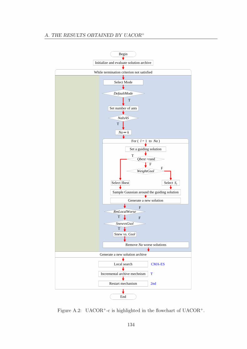
A. THE RESULTS OBTAINED BY UACOR+
b
Qbest >rand
WeightGsol
Set a guiding solution
Sample Gaussian around the guiding solution
Initialize and evaluate solution archive
RmLocalWorse
T
SnewvsGsol
DefaultMode
T
End
Select Sbest
T
While termination criterion not satisfied
For ( l = 1 to Na )
NaIsAS
T
Generate a new solution
T
F
Local search
Incremental archive mechnism
Restart mechanism
Begin
F
Remove Na worse solutions
F
Select lS
Generate a new solution archive
Select Mode
Set number of ants
Na k
F
Snew vs. Gsol
CMA-ES
2nd
T
Figure A.2: UACOR+-c is highlighted in the flowchart of UACOR+.
134

AC
Or−
s
DA
CO
r−s
IAC
Or−
mts
ls1
−s
UACOR+−s
1e−14
1e−09
1e−04
1e+01
1e+06
+ + +Optima 0 1 8 14
Ave
rage
Err
ors
of
Fitn
ess V
alu
e
Arc
hS
ize
=1
Arc
hS
ize=
50
Arc
hS
ize=
10
0
ArchSize=inc
1e−14
1e−09
1e−04
1e+01
1e+06
+ +Optima 6 7 9 14
Ave
rage
Err
ors
of
Fitn
ess V
alu
e
Figure A.3: The box-plots show the distribution of the average errors obtained onthe 19 SOCO benchmark functions of dimension 100. The left plot compares theperformance of UACOR+-s with ACOR-s, DACOR-s and IACOR-Mtsls1-s. Theright plot shows the benefit of the incremental archive size used in UACOR+-s. A+ symbol on top of each box-plot denotes a statistically significant difference atthe 0.05 α-level between the results obtained by the indicated algorithm and thoseobtained with UACOR+-s. The absence of a symbol means that the difference isnot statistically significant. The numbers on top of a box-plot denote the number ofthe averages below the optimum threshold 10−14 found by the indicated algorithms.
135

A. THE RESULTS OBTAINED BY UACOR+
DE
CH
C
IPO
P−
CM
A−
ES
SO
UP
DE
DE
−D
40
−M
m
GO
DE
Ga
DE
jDE
lsco
p
Sa
DE
−M
MT
S
MO
S−
DE
MA
−S
SW
RP
SO
−vm
IPS
O−
Pow
ell
Evo
PR
Op
t
EM
32
3
VX
QR
1
UACOR
+−s
1e−14
1e−09
1e−04
1e+01
1e+06
+ + + + + + + + + + + +Optima 6 0 2 8 9 6 9 10 12 13 8 4 5 0 4 5 14
Ave
rag
e E
rro
rs o
f F
itn
ess V
alu
e
16 algorithms in SOCO
Figure A.4: The box-plot show the distribution of the average errors obtained onthe 19 SOCO benchmark functions of dimension 100. The results obtained by thethree reference algorithms (left), 13 algorithms (middle) published in SOCO andUACOR+-s (right) are shown on the plot. The line at the bottom of the boxplotrepresents the optimum threshold (10−14). A + symbol on top of the two box-plot denotes a statistically significant difference at the 0.05 α-level between theresults obtained with the indicated algorithm and those obtained with UACOR+-s detected with a Friedman test and its associated post test on the 17 algorithms.The absence of a symbol means that the difference is not significant. The numberson top of a box-plot denote the number of averages below the optimum threshold10−14 found by the indicated algorithms.
136

Table A.2: The average errors obtained by ACOR-s, DACOR-s, IACOR-Mtsls1-s,MOS-DE and UACOR+-s for each SOCO function. The numbers in parenthesis atthe bottom of the table represent the number of times an algorithm is better, equal orworse, respectively, than UACOR+-s. Error values lower than 10−14 are approximatedto 10−14. The average errors that correspond to a better result between MOS-DEand UACOR+-c are highlighted.
Dim fsoco ACOR-s DACOR-s IACOR-Mtsls1-s MOS-DE UACOR+-s
100
fsoco1 5.32E−14 1.00E−14 1.00E−14 1.00E−14 1.00E−14fsoco2 2.77E+01 3.82E+01 5.27E−12 2.94E−12 6.86E−11fsoco3 1.96E+02 2.86E+03 4.77E+02 2.03E+01 3.02E+02fsoco4 6.34E+02 3.89E+02 1.00E−14 1.00E−14 1.00E−14fsoco5 2.96E−04 4.96E−01 1.00E−14 1.00E−14 1.00E−14fsoco6 2.04E−08 3.49E+00 1.00E−14 1.00E−14 1.00E−14fsoco7 9.94E−10 5.01E−01 1.00E−14 1.00E−14 1.00E−14fsoco8 4.39E+04 2.28E+04 1.39E+00 9.17E−02 1.34E+00fsoco9 4.78E+00 1.84E+02 1.62E−01 1.00E−14 1.00E−14fsoco10 2.75E+00 2.09E+01 1.00E−14 1.00E−14 1.00E−14fsoco11 3.96E+00 1.90E+02 1.67E−01 1.00E−14 1.00E−14fsoco12 1.13E+01 2.39E+02 4.01E−02 1.00E−14 1.00E−14fsoco13 1.47E+02 3.92E+02 4.19E+01 1.75E+01 3.12E+01fsoco14 3.40E+02 2.40E+02 9.23E+00 1.68E−11 1.00E−14fsoco15 5.89E−01 4.41E+00 1.00E−14 1.00E−14 1.00E−14fsoco16 1.61E+00 4.18E+02 4.24E−01 1.00E−14 1.00E−14fsoco17 6.27E+01 6.65E+02 8.40E+01 1.43E+01 4.08E+01fsoco18 1.57E+01 1.17E+02 1.07E−01 1.00E−14 1.00E−14fsoco19 1.48E+00 1.61E+01 1.00E−14 1.00E−14 1.00E−14
By fsoco (1, 0, 18)† (0, 1, 18)† (1, 8, 10)† (5, 13, 1)
† denotes a significant difference between the corresponding algorithm and UACOR+-s by a Fried-man test at the 0,05 α-level over the distribution of average errors of ACOR-s, DACOR-s, IACOR-Mtsls1-s and UACOR+-s.
137

A. THE RESULTS OBTAINED BY UACOR+
Table A.3: The average errors obtained by ACOR-c, DACOR-c, IACOR-Mtsls1-c, IPOP-CMA-ES and UACOR+-c for each CEC’05 function. The numbers in parenthesis at thebottom of the table represent the number of times an algorithm is better, equal or worse,respectively, compared to UACOR+-c. Error values lower than 10−8 are approximated to10−8. The average errors that correspond to a better result between IPOP-CMA-ES andUACOR+-c are highlighted.
Dim fcec ACOR-c DACOR-c IACOR-Mtsls1-c IPOP-CMA-ES UACOR+-c
30
fcec1 1.00E−08 1.00E−08 1.00E−08 1.00E−08 1.00E−08fcec2 1.00E−08 4.74E+00 1.00E−08 1.00E−08 1.00E−08fcec3 3.88E+05 4.21E+06 2.19E+05 1.00E−08 1.00E−08fcec4 2.75E−04 2.62E+02 9.45E+03 1.11E+04 1.14E+03fcec5 1.00E−08 1.00E−08 6.79E−08 1.00E−08 1.00E−08fcec6 8.99E+00 2.50E+01 1.64E+02 1.00E−08 1.00E−08fcec7 1.80E−02 1.54E−02 1.00E−02 1.00E−08 1.00E−08fcec8 2.00E+01 2.02E+01 2.00E+01 2.01E+01 2.00E+01fcec9 2.50E+01 6.35E+01 1.00E−08 9.38E−01 2.95E+01fcec10 4.51E+01 6.58E+01 1.19E+02 1.65E+00 2.91E+01fcec11 3.75E+01 3.19E+01 2.36E+01 5.48E+00 3.82E+00fcec12 3.59E+03 1.92E+04 7.89E+03 4.43E+04 2.21E+03fcec13 3.67E+00 4.57E+00 1.28E+00 2.49E+00 2.26E+00fcec14 1.25E+01 1.34E+01 1.32E+01 1.29E+01 1.32E+01fcec15 3.40E+02 3.28E+02 2.48E+02 2.08E+02 1.92E+02fcec16 1.33E+02 1.93E+02 2.49E+02 3.50E+01 6.14E+01fcec17 1.49E+02 1.81E+02 3.35E+02 2.91E+02 2.87E+02fcec18 9.12E+02 9.07E+02 9.02E+02 9.04E+02 8.73E+02fcec19 9.11E+02 9.07E+02 8.92E+02 9.04E+02 8.83E+02fcec20 9.12E+02 9.07E+02 8.97E+02 9.04E+02 8.78E+02fcec21 5.38E+02 5.00E+02 5.12E+02 5.00E+02 5.00E+02fcec22 9.08E+02 8.70E+02 9.90E+02 8.03E+02 8.57E+02fcec23 5.75E+02 5.35E+02 5.66E+02 5.34E+02 5.34E+02fcec24 2.27E+02 7.85E+02 1.26E+03 9.10E+02 3.41E+02fcec25 2.19E+02 2.31E+02 5.60E+02 2.11E+02 2.63E+02
50
fcec1 1.00E−08 1.00E−08 1.00E−08 1.00E−08 1.00E−08fcec2 1.80E−04 2.61E+03 4.08E−07 1.00E−08 1.00E−08fcec3 6.68E+05 6.72E+06 5.60E+05 1.00E−08 1.00E−08fcec4 8.36E+03 4.69E+04 5.33E+04 4.68E+05 1.69E+04fcec5 2.23E−05 2.02E−01 7.95E−07 2.85E+00 1.00E−08fcec6 2.92E+01 5.18E+01 1.73E+02 1.00E−08 1.00E−08fcec7 9.93E−03 1.08E−02 4.53E−03 1.00E−08 1.00E−08fcec8 2.00E+01 2.02E+01 2.00E+01 2.01E+01 2.01E+01fcec9 4.82E+01 1.15E+02 1.00E−08 1.39E+00 8.18E+01fcec10 9.77E+01 1.42E+02 2.83E+02 1.72E+00 7.45E+01fcec11 7.30E+01 5.81E+01 4.63E+01 1.17E+01 1.07E+01fcec12 2.74E+04 1.07E+05 1.47E+04 2.27E+05 1.27E+04fcec13 7.24E+00 1.06E+01 2.13E+00 4.59E+00 4.76E+00fcec14 2.24E+01 2.29E+01 2.26E+01 2.29E+01 2.31E+01fcec15 3.26E+02 3.61E+02 2.64E+02 2.04E+02 1.74E+02fcec16 1.10E+02 1.64E+02 2.89E+02 3.09E+01 7.01E+01fcec17 1.62E+02 2.45E+02 5.65E+02 2.34E+02 3.17E+02fcec18 9.33E+02 9.26E+02 9.31E+02 9.13E+02 9.08E+02fcec19 9.34E+02 9.27E+02 9.18E+02 9.12E+02 8.76E+02fcec20 9.36E+02 9.27E+02 9.19E+02 9.12E+02 8.64E+02fcec21 5.39E+02 9.82E+02 5.12E+02 1.00E+03 5.00E+02fcec22 9.48E+02 9.07E+02 1.06E+03 8.05E+02 8.92E+02fcec23 5.56E+02 1.02E+03 5.53E+02 1.01E+03 5.41E+02fcec24 2.94E+02 9.06E+02 1.40E+03 9.55E+02 8.26E+02fcec25 2.63E+02 3.39E+02 9.52E+02 2.15E+02 3.53E+02
By fcec (13, 5, 32)† (6, 4, 40)† (6, 5, 39)† (14, 14, 22)
† denotes a significant difference between the corresponding algorithm and UACOR+-s by a Friedmantest at the 0,05 α-level over the distribution of average errors of ACOR-c, DACOR-c, IACOR-Mtsls1-cand UACOR+-c.
138

Table A.4: The average errors obtained by HDDE, Pro-JADE, Pro-SaDE, Pro-DEGL, ABC-MRand UACOR+-c for for each CEC’05 function. The numbers in parenthesis at the bottom of thetable represent the number of times an algorithm is better, equal or worse, respectively, comparedto UACOR+-c. Error values lower than 10−8 are approximated to 10−8. The lowest average errorsvalues are highlighted.
Dim fcec HDDE Pro-JADE Pro-SaDE Pro-DEGL ABC-MR UACOR+-c
30
fcec1 1.00E−08 1.00E−08 1.00E−08 1.00E−08 1.00E−08 1.00E−08fcec2 8.13E+00 1.00E−08 1.00E−08 1.00E−08 1.00E−08 1.00E−08fcec3 2.31E+06 1.85E+04 2.28E+06 4.20E+04 2.20E+05 1.00E−08fcec4 1.33E+02 1.00E−08 2.00E−05 1.00E−08 1.00E−08 1.14E+03fcec5 7.66E+02 5.90E+01 5.51E+01 1.91E+01 6.02E+03 1.00E−08fcec6 3.19E+01 1.89E+01 1.36E+00 1.20E+00 1.38E+02 1.00E−08fcec7 4.70E+03 4.70E+03 4.70E+03 4.69E+03 1.49E−02 1.00E−08fcec8 2.09E+01 2.09E+01 2.10E+01 2.09E+01 2.09E+01 2.00E+01fcec9 3.91E+00 1.00E−08 1.00E−08 3.58E+01 6.60E+01 2.95E+01fcec10 6.01E+01 8.18E+01 1.01E+02 5.18E+01 2.01E+02 2.91E+01fcec11 2.57E+01 3.01E+01 3.37E+01 2.01E+01 3.56E+01 3.82E+00fcec12 7.86E+03 2.63E+04 1.48E+03 2.35E+04 9.55E+04 2.21E+03fcec13 2.04E+00 3.32E+00 2.95E+00 3.40E+00 1.07E+01 2.26E+00fcec14 1.27E+01 1.29E+01 1.31E+01 1.24E+01 1.88E−01 1.32E+01fcec15 3.17E+02 3.71E+02 3.86E+02 3.53E+02 2.88E+02 1.92E+02fcec16 8.58E+01 1.14E+02 6.97E+01 1.76E+02 3.06E+02 6.14E+01fcec17 1.01E+02 1.45E+02 7.20E+01 1.60E+02 3.01E+02 2.87E+02fcec18 9.03E+02 8.60E+02 8.56E+02 9.09E+02 8.12E+02 8.73E+02fcec19 9.04E+02 8.90E+02 8.67E+02 9.10E+02 8.17E+02 8.83E+02fcec20 9.04E+02 8.96E+02 8.52E+02 9.10E+02 8.23E+02 8.78E+02fcec21 5.00E+02 5.06E+02 5.00E+02 6.79E+02 6.42E+02 5.00E+02fcec22 8.76E+02 8.95E+02 9.09E+02 8.94E+02 9.04E+02 8.57E+02fcec23 5.34E+02 5.00E+02 5.00E+02 6.77E+02 8.20E+02 5.34E+02fcec24 2.00E+02 2.00E+02 2.00E+02 7.77E+02 2.01E+02 3.41E+02fcec25 1.28E+03 1.67E+03 1.63E+03 1.64E+03 2.00E+02 2.63E+02
50
fcec1 1.00E−08 1.00E−08 1.00E−08 1.00E−08 1.00E−08 1.00E−08fcec2 3.30E+02 1.00E−08 7.40E−04 1.00E−08 1.00E−08 1.00E−08fcec3 4.44E+06 4.30E+04 7.82E+05 1.93E+05 1.13E+06 1.00E−08fcec4 2.94E+03 3.19E−01 6.64E+01 1.08E−01 3.82E+02 1.69E+04fcec5 3.22E+03 1.83E+03 1.95E+03 2.23E+03 1.03E+04 1.00E−08fcec6 5.74E+01 1.04E+01 1.15E+01 8.77E−01 2.47E+03 1.00E−08fcec7 6.20E+03 6.20E+03 6.20E+03 6.20E+03 8.10E−01 1.00E−08fcec8 2.11E+01 2.10E+01 2.11E+01 2.11E+01 2.11E+01 2.01E+01fcec9 1.87E+01 2.77E+01 6.61E−01 7.94E+01 2.59E+02 8.18E+01fcec10 1.13E+02 1.99E+02 6.23E+01 9.24E+01 4.58E+02 7.45E+01fcec11 5.19E+01 6.03E+01 6.61E+01 6.14E+01 7.03E+01 1.07E+01fcec12 3.84E+04 9.45E+04 7.34E+03 6.32E+04 8.88E+05 1.27E+04fcec13 4.36E+00 9.14E+00 6.90E+00 5.41E+00 3.50E+01 4.76E+00fcec14 2.23E+01 2.26E+01 2.28E+01 2.26E+01 2.32E+01 2.31E+01fcec15 2.62E+02 3.80E+02 3.96E+02 3.44E+02 2.52E+02 1.74E+02fcec16 1.05E+02 1.44E+02 4.85E+01 1.63E+02 3.39E+02 7.01E+01fcec17 1.15E+02 1.92E+02 9.36E+01 1.94E+02 3.08E+02 3.17E+02fcec18 9.17E+02 9.26E+02 9.05E+02 9.28E+02 9.85E+02 9.08E+02fcec19 9.16E+02 9.32E+02 8.97E+02 9.28E+02 9.70E+02 8.76E+02fcec20 9.16E+02 9.33E+02 9.11E+02 9.29E+02 9.70E+02 8.64E+02fcec21 7.37E+02 5.00E+02 5.00E+02 9.50E+02 8.34E+02 5.00E+02fcec22 9.01E+02 9.49E+02 9.60E+02 9.28E+02 8.75E+02 8.92E+02fcec23 7.85E+02 5.00E+02 5.06E+02 9.35E+02 5.71E+02 5.41E+02fcec24 2.00E+02 2.00E+02 2.00E+02 6.81E+02 2.01E+02 8.26E+02fcec25 1.37E+03 1.71E+03 1.69E+03 1.67E+03 2.01E+02 3.53E+02
By fcec (12, 4, 34)† (13, 5, 32)† (20, 5, 25)† (8, 4, 38)† (12, 4, 34)†
† denotes a significant difference between the corresponding algorithm and UACOR+-c by a Friedman test atthe 0,05 α-level over the distribution of average errors of HDDE, Pro-JADE, Pro-SaDE, Pro-DEGL, ABC-MRand UACOR+-c.
139

A. THE RESULTS OBTAINED BY UACOR+
Tab
leA
.5:G
ivenare
the
averageran
k,
the
num
ber
ofop
timum
thresh
olds
reached
,an
dth
enum
ber
oftim
esth
elow
estaverage
errorsreach
edby
eachalgorith
mpresen
tedin
Tab
leA
.4.In
addition
,w
egive
the
publication
source
foreach
reference
algorithm
.
Algorith
ms
Averag
eR
ankin
gN
um
of
Op
tima
Nu
mof
lowest
average
errorvalu
esP
ub
licationS
ources
UA
CO
R+
-c2.5
212
25
Pro-S
aDE†
3.224
17
IEE
ET
EC
,2011
Pro-J
AD
E†
3.546
11
IEE
ET
EC
,2011
HD
DE†
3.542
8IE
EE
TE
C,
2011P
ro-DE
GL†
3.895
6IE
EE
TE
C,
2011A
BC
-MR†
4.295
12
Inform
ationS
ciences,
2012
†d
enotes
asign
ifican
td
ifferen
ceb
etween
the
corresp
on
din
galg
orith
man
dU
AC
OR
+-c
by
aF
riedm
antest
atth
e0,05
α-level
overth
ed
istribu
tionof
avera
ge
errors
of
HD
DE
,P
ro-J
AD
E,
Pro
-SaD
E,
Pro-D
EG
L,
AB
C-M
Ran
dU
AC
OR
+-c.
140

Appendix B
Mathematical formulation of engineering problems
In Appendix B, we give an explicit definition of the engineering problems that we
used for benchmark the ACOMV and the CESMV algorithms in Chapter 5.
Welded beam design problem case A
The mathematical formulation of the welded beam design problem is given in
Table B.1. The schematic view of this problem is shown in Fig. B.1
Welded beam design problem case B
The welded beam design problem case B is a variation of case A. It is extended to
include two types of welded joint configuration and four possible beam materials.
The changed places are shown in Equation B.1 and Table B.2.
Figure B.1: Schematic view of welded beam design problem case A [Kayhan et al.,2010].
141

B. MATHEMATICAL FORMULATION OF ENGINEERING PROBLEMS
Table B.1: The mathematical formulation of welded beam design problem case A.
min f(~x) = 1.10471x21x2 + 0.04811x3x4 (14 + x2)
g1 τ(~x)− τmax ≤ 0g2 σ(~x)− σmax ≤ 0g3 x1 − x4 ≤ 0g4 0.10471x2
1 + 0.04811x3x4 (14 + x2)− 5 ≤ 0g5 0.125− x1 ≤ 0g6 δ(~x)− δmax ≤ 0g7 P − Pc(~x) ≤ 0g8 0.1 ≤ x1, x4 ≤ 2.0g9 0.1 ≤ x2, x3 ≤ 10.0
where τ(~x) =√
(τ ′)2 + 2τ ′τ ′′ x22R
+ (τ ′′)2
τ ′ = P√2x1x2
, τ ′′ = MRJ,M = P (L+ x2
2)
R =
√x224
+ (x1+x32
)2
J = 2
√2x1x2
[x2212
+(x1+x3
2
)2]
σ(~x) = 6PLx4x
23, δ(~x) = 4PL3
Ex33x4
Pc(~x) =4.013E
√x23x6
436
L2
(1− x3
2L
√E4G
)P = 6 000lb, L = 14in., E = 30× 106psi,G = 12× 106psi
τmax = 1 360psi, σmax = 30 000psi, δmax = 0.25in.
min f(~x) = (1 + c1)x21x2 + c2 x3x4 (14 + x2)
σ(~x)− S ≤ 0
J = 2√
2x1x2
[x22
12 +(x1+x3
2
)2], if x6 : twoside
J = 2√
2x1
[(x1+x2+x3)
3
12
], if x6 : fourside
τmax = 0.577 · S
(B.1)
Table B.2: Material properties for the welded beam design problem case B
Methods x5 S(103psi) E(106psi) G(106psi) c1 c2Steel 30 30 12 0.1047 0.0481
Cast iron 8 14 6 0.0489 0.0224Aluminum 5 10 4 0.5235 0.2405
Brass 8 16 6 0.5584 0.2566
Pressure vessel design problem
The pressure vessel design problem requires designing a pressure vessel consisting
of a cylindrical body and two hemispherical heads such that the manufacturing
cost is minimized subject to certain constraints. The schematic picture of the
vessel is presented in Fig. B.2. There are four variables for which values must be
chosen: the thickness of the main cylinder Ts, the thickness of the heads Th, the
142

Table B.3: The mathematical formulation the cases (A, B, C and D) of the pressurevessel design problem.
No Case A Case B Case C Case Dmin f = 0.6224TsRL+ 1.7781ThR
2 + 3.1611T 2s L+ 19.84T 2
sRg1 −Ts + 0.0193R ≤ 0g2 −Th + 0.00954R ≤ 0
g3 −π R2L− 43π R3 + 750 · 1728 ≤ 0
g4 L− 240 ≤ 0g5 1.1 ≤ Ts ≤ 12.51.125 ≤ Ts ≤ 12.51 ≤ Ts ≤ 12.5 0 ≤ Ts ≤ 100g6 0.6 ≤ Th ≤ 12.5 0.625 ≤ Th ≤ 12.5 0 ≤ Th ≤ 100g7 0.0 ≤ R ≤ 240 10 ≤ R ≤ 200g8 0.0 ≤ L ≤ 240 10 ≤ L ≤ 200
inner radius of the main cylinder R, and the length of the main cylinder L. While
variables R and L are continuous, the thickness for variables Ts and Th may be
chosen only from a set of allowed values, these being the integer multiples of 0.0625
inch. The mathematical formulation of the four cases A, B, C and D is given in
Table B.3.
Coil spring design problem
The problem consists in designing a helical compression spring that holds an axial
and constant load. The objective is to minimize the volume of the spring wire
used to manufacture the spring. A schematic of the coil spring to be designed is
shown in Fig. B.3. The decision variables are the number of spring coils N , the
outside diameter of the spring D, and the spring wire diameter d. The number of
coils N is an integer variable, the outside diameter of the spring D is a continuous
one, and finally, the spring wire diameter d is a discrete variable, whose possible
values are given in Table B.4. The mathematical formulation is in Table B.5.
Figure B.2: Schematic view of the pressure vessel to be designed.
143

B. MATHEMATICAL FORMULATION OF ENGINEERING PROBLEMS
Figure B.3: Schematic view of the coil spring to be designed.
Table B.4: Standard wire diameters available for the spring coil.
Allowed wire diameters [inch]0.0090 0.0095 0.0104 0.0118 0.0128 0.01320.0140 0.0150 0.0162 0.0173 0.0180 0.02000.0230 0.0250 0.0280 0.0320 0.0350 0.04100.0470 0.0540 0.0630 0.0720 0.0800 0.09200.1050 0.1200 0.1350 0.1480 0.1620 0.17700.1920 0.2070 0.2250 0.2440 0.2630 0.28300.3070 0.3310 0.3620 0.3940 0.4375 0.5000
Table B.5: The mathematical formulation for the coil spring design problem.
min fc(N,D, d) =π2Dd2(N+2)
4Constraint
g18CfFmaxD
π d3− S ≤ 0
g2 lf − lmax ≤ 0g3 dmin − d ≤ 0g4 D −Dmax ≤ 0
g5 3.0− Dd≤ 0
g6 σp − σpm ≤ 0
g7 σp +Fmax−Fp
K+ 1.05(N + 2)d− lf ≤ 0
g8 σw −Fmax−Fp
K≤ 0
where Cf =4 D
d−1
4 Dd−4
+ 0.615 dD
K = Gd4
8ND3
σp =Fp
K
lf = FmaxK
+ 1.05(N + 2)d
Thermal insulation systems design problem
The schema of a thermal insulation system is shown in Fig. B.4. Such a thermal
insulation system is characterized by the number of intercepts, the locations and
temperatures of the intercepts, and the types of insulators allocated between each
pair of neighboring intercepts. In the thermal insulation system, heat intercepts
are used to minimize the heat flow from a hot to a cold surface. The heat is
intercepted by imposing a cooling temperature Ti at locations xi, i = 1, 2, ..., n.
144

Figure B.4: Schematic view of the thermal insulation system.
The basic mathematical formulation of the classic model of thermal insulation
systems is defined in Table B.6. The effective thermal conductivity k of all these
insulators varies with the temperature and does so differently for different materi-
als. Considering that the number of intercepts n is defined in advance, and based
on the model presented (n=10), we may define the following problem variables:
• Ii ∈M, i = 1, ..., n + 1 — the material used for the insulation between the
(i− 1)-th and the i-th intercepts (from a set of M materials).
• ∆xi ∈ R+, i = 1, ..., n + 1 — the thickness of the insulation between the
(i− 1)-th and the i-th intercepts.
• ∆Ti ∈ R+, i = 1, ..., n + 1 — the temperature difference of the insulation
between the (i− 1)-th and the i-th intercepts.
This way, there are n+ 1 categorical variables chosen from a set of M of available
materials. The remaining 2n+ 2 variables are continuous.
Table B.6: The mathematical formulation for the coil spring design problem.
f(x,T) =∑ni=1 Pi
=∑ni=1 ACi
(ThotTi− 1)( ∫ Ti+1
TikdT
∆xi−
∫ Ti
Ti−1kdT
∆xi−1
)Constraint
g1 ∆xi ≥ 0, i = 1, ..., n+ 1g2 Tcold ≤ T1 ≤ T2 ≤ ... ≤ Tn−1 ≤ Tn ≤ Thot
g3∑n+1i=1 ∆xi = L
where C = 2.5 if T ≥ 71 KC = 4 if 71 K > T > 4.2 K
C = 5 if T ≤ 4.2 K
145

B. MATHEMATICAL FORMULATION OF ENGINEERING PROBLEMS
146

Appendix C
A note on the bound constraints handling for the CEC’05benchmark set
The benchmark functions and some of the algorithms proposed for the special
session on real parameter optimization of CEC’05 play an important role in the
assessment of the state of the art in the continuous optimization field. In this note
we first show that, if boundary constraints are not enforced, state-of-the-art algo-
rithms produce on a majority of the CEC’05 benchmark functions infeasible best
candidate solutions, even though the optima of 23 out of the 25 CEC’05 functions
are within the specified bounds. This observation has important implications on
algorithm comparisons. In fact, this note also draws the attention to the fact that
authors may have drawn wrong conclusions from experiments using the CEC’05
problems.
C.1 Introduction
The special session on real parameter optimization of CEC’05 has played an im-
portant role in evolutionary computation and other affine fields for two reasons.
First, it provided a set of 25 scalable benchmark functions that anyone can use to
evaluate the performance of new algorithms. Those 25 functions have become a
standard benchmark set that researchers use to compare algorithms. The central
role that this benchmark function set currently plays is also illustrated by the more
than 600 citations in google scholar (as of April 2013) to the original technical re-
port that introduced the benchmark function set [Suganthan et al., 2005]. Second,
it served to assess the state of the art in continuous optimization. In particular,
the best performing algorithm of the special session, IPOP-CMA-ES [Auger and
Hansen, 2005], is since then considered to be a representative of the state of the
art in continuous optimization. Consequently, it is nowadays standard practice to
147

C. A NOTE ON THE BOUND CONSTRAINTS HANDLING FOR THECEC’05 BENCHMARK SET
compare the results of a new algorithm to the published results of IPOP-CMA-ES.
In the definition of the CEC’05 benchmark functions it is stated that each com-
ponent of the solution S must be a value in the closed interval [A,B], with A < B.
There are two exceptions, which are functions f7 and f25, where the given interval
specifies only an initialization range, and not a boundary constraint. For the other
23 functions, their global optima are within the feasible search space area as defined
by the bound constraints; on functions f8 and f20, the global optima are known to
be on the bounds. We used the C implementation of IPOP-CMA-ES available from
Hansen’s website, http://www.lri.fr/~hansen/cmaes_inmatlab.html. This C
version of IPOP-CMA-ES does not use an explicit bound constraint handling
mechanism. When running this code (without bound constraint handling) on the
CEC’05 benchmark functions, we noticed that on a majority of the benchmark
functions the best solutions found do violate the bound constraints even though
their global optima are known to be inside the bounds for 23 of the 25 functions.
While it is known that this can happen on other functions, for example, Schwe-
fel’s sine root function [Schwefel, 1981] whose global optimum is outside the usual
feasible search space defined by bound constraints, we were surprised by the high
frequency with which this phenomenon occurs on the CEC’05 benchmark function
set.
This observation raises the more general and critical issue of validity of many
of the published results that rely on the CEC’05 benchmark set. In fact, most
articles do not explicitly report whether a bound constraint handling mechanism
was used, and if they do, many do not describe it. Perhaps more importantly,
claims about algorithms with a statistically significantly better performance than
IPOP-CMA-ES (e.g., [Molina et al., 2010a, Muller et al., 2009] may not be valid
because the comparison that supports those claims may include algorithms that
enforce bound constraints and algorithms that do not.
To show how misleading such a comparison can be, we report our experimental
evidence on the impact of the handling of bound constraints. We evaluate two
variants of the C version of IPOP-CMA-ES. The first is the version in which the
bound constraints are never enforced (ncb for “never clamp bounds”; we refer to
this version as IPOP-CMA-ES-ncb in what follows). The second is a version in
which we introduce a mechanism to enforce bound constraints in the C code from
Hansen’s webpage. In particular, we clamp dimension by dimension a variable’s
value that is outside the variable’s feasible domain to the closest boundary value;
that is, if xi < A we set xi = A and if xi > B we set xi = B before evaluat-
ing these solutions and continuing with the algorithm execution (acb for “always
148
clamp bounds”; this version is referred to as IPOP-CMA-ES-acb). The same two
variants where bound constraints are never enforced or always enforced by clamp-
ing infeasible solutions to the nearest solutions on the bounds are tested using
a memetic algorithm, MA-LSCh-CMA [Molina et al., 2010a], which is a recent
memetic algorithm that uses CMA-ES as a local search.
C.2 Experiments on enforcing bound constraints
In this first set of experiments, we examine the impact of bound handling on
the performance of the C version of IPOP-CMA-ES. For the experiments on the
CEC’05 benchmark functions, we followed the protocol described in [Suganthan
et al., 2005], that is, we ran IPOP-CMA-ES using its default parameter settings 25
times on each function and recorded the evolution of the objective function value
with respect to the number of function evaluations used. The maximum number
of function evaluations was 10000 ·D, where D ∈ 10, 30, 50 is the dimensionality
of a function. The algorithm stops when the maximum number of evaluations is
reached or the error obtained is lower than 10−8. Error values lower than this
optimum threshold are considered equal to 10−8, and these values therefore are
clamped to 10−8 for consistency.
We compare IPOP-CMA-ES-ncb and IPOP-CMA-ES-acb in Table C.1.1 The
two-sided Wilcoxon matched-pairs signed-rank test at the 0.05 level of the error
of first type was used to check for statistical differences on each function. On
the majority of the functions, that is in 14 to 17 functions depending on the
dimensionality, IPOP-CMA-ES-ncb obtains final solutions outside the bounds. In
most of the cases where infeasible solutions are found, all 25 runs return final
solutions outside the bounds. We have observed statistically significant differences
between IPOP-CMA-ES-ncb and IPOP-CMA-ES-acb when the final solutions of
IPOP-CMA-ES-ncb are outside the bounds. Surprisingly, while a priori we would
expect that IPOP-CMA-ES-ncb gives worse results than IPOP-CMA-ES-acb on
functions where the optima are known to be inside the bounds, IPOP-CMA-ES-
ncb in fact outperforms IPOP-CMA-ES-acb in six functions (f9, f12, f18, f19, f20
and f22 for dimensions 30 and 50). In all these functions, except f9, all solutions
obtained by IPOP-CMA-ES-ncb are outside the bounds.
Analogously, Table C.2 shows the performance of ncb and acb for MA-LSCh-
1The results in Table C.1 and in Tables C.2 and C.3 are based on average errors. In thesupplementary pages to this chapter at http://iridia.ulb.ac.be/supp/IridiaSupp2011-013additional tables are given that show the median results and more detailed information such asthe best, 0.25 quartile, median, 0.75 quartile and worst error values for each function.
149

C. A NOTE ON THE BOUND CONSTRAINTS HANDLING FOR THECEC’05 BENCHMARK SET
CMA (MA-LSCh-CMA is run using default parameter settings). Again, version
ncb obtains many final solutions outside the bounds, for dimensions 30 and 50
this is the case on 18 and 19 functions, respectively.2 Taking the 50 dimensional
benchmark functions as an example, all functions for which MA-LSCh-CMA-ncb
outperforms MA-LSCh-CMA-acb are cases in which all solutions obtained by MA-
LSCh-CMA-ncb are outside the bounds (f5, f11, f12, f15, f18, f19, f20 and f22).
C.3 The impact of bound handling on algorithm compar-
isons
We now focus on the comparison of the average errors between PS-CMA-ES
[Muller et al., 2009], MA-LSCh-CMA [Molina et al., 2010a], IPOP-CMA-ES-ncb
and IPOP-CMA-ES-05 in Table C.3. IPOP-CMA-ES-05 uses the Matlab version
of CMA-ES and was used to generate the results for the CEC’05 benchmark func-
tions presented in [Auger and Hansen, 2005]; it handles bound constraints by an
approach based on penalty functions, which is described in [Hansen et al., 2009c].
PS-CMA-ES and MA-LSCh-CMA are examples of algorithms that have been re-
ported to outperform IPOP-CMA-ES-05; they use CMA-ES as a local search oper-
ator inside a particle swarm optimization algorithm and a real-coded steady state
genetic algorithm, respectively.
In fact, Table C.3 shows that PS-CMA-ES, MA-LSCh-CMA, but also IPOP-
CMA-ES-ncb, are superior to IPOP-CMA-ES-05 on 30 and 50 dimensions in the
sense that they find more often better average errors than IPOP-CMA-ES-05.
However, there is an interesting pattern related to the fact whether IPOP-CMA-
ES-ncb has the final solutions outside the bounds or not. Let us focus on the
cases where IPOP-CMA-ES-ncb obtains all solutions outside the bounds and sta-
tistically significantly improves over IPOP-CMA-ES-05 (as indicated by the “<”
symbol in Table C.3). In many such cases, PS-CMA-ES does obtain the same
average errors (see, for example, functions f18–f20 and f24 for both, 30 and 50
dimensions and function f22 for 50 dimensions), or very similar values (see, for
example, functions f22 and f23 for 50 dimensions); such cases are underlined in
Table C.3. A similar pattern also arises for the published results of the MA-LSCh-
CMA algorithm. Interestingly, MA-LSCh-CMA checks bound constraints only for
2Note that for both, IPOP-CMA-ES-ncb and MA-LSCh-CMA-ncb, the fraction of functionsfor which at least once in 25 runs an infeasible solution is found, increases with the dimensionalityof the functions. The probable reason for this effect is that for a solution to be infeasible it sufficesthat one single variable takes a value outside the boundary constraints—such an effect occursmore likely for higher dimensional functions.
150
the solutions generated by the steady-state GA part but not for solutions returned
by the CMA-ES local search. After re-running the publicly available version of
MA-LSCh-CMA, we found that it returns on several functions infeasible final solu-
tions (as indicated by the symbols and in Table C.3). This knowledge together
with the similar pattern of the average errors puts at least serious doubts on the
fact whether the average errors reported in [Muller et al., 2009] correspond all to
solutions that are inside the bounds. This analysis shows that claims of superiority
of one algorithm over another may in fact not be valid if the algorithms involved
do not all enforce bound constraints.
C.4 Conclusions
In this note, we show that lack of enforcement of bound constraints greatly influ-
ences the feasibility of the solutions on the CEC’05 benchmark function suite, as
it is observed in IPOP-CMA-ES and MA-LSCh-CMA. Without explicit enforce-
ment of bound constrains, surprisingly often infeasible solutions are obtained on
the CEC’05 benchmark functions; in many cases, these infeasible solutions are
better than the best feasible solutions found if bound constraints are enforced
even though it is known that on most functions the optimal solutions are within
the bounds. This issue points toward a significant impact on CEC’05 benchmark
functions for what concerns algorithm comparison, but it certainly may apply also
to other benchmark sets [Hansen et al., 2009a, Herrera et al., 2010, Tang et al.,
2007]. In particular, claims about superior performance of one algorithm over
another may be erroneous due to the generation of infeasible solutions with re-
spect to bound constraints. To avoid possible doubts about the feasibility of the
solutions, we strongly recommend that in the future every paper that reports re-
sults on the CEC’05 benchmark function suite but also on other benchmark suites
should (i) explicitly describe the used bound handling mechanism, (ii) explicitly
check the feasibility of the final solutions3, and (iii) present the final solutions
at least in supplementary pages to the paper to avoid misinterpretations. All
the solutions generated by the algorithms discussed in this note are available at
http://iridia.ulb.ac.be/supp/IridiaSupp2011-013.
3We notice that many bound handling mechanisms use penalty approaches such as the onealso used by [Hansen et al., 2009c]. However, it still is possible to obtain infeasible solutions ifbound constraints are not explicitly enforced, no matter what penalty approach is used as thebound handling mechanism.
151

C. A NOTE ON THE BOUND CONSTRAINTS HANDLING FOR THECEC’05 BENCHMARK SET
Table C.1: The comparison between IPOP-CMA-ES-ncb and IPOP-CMA-ES-acb over 25independent runs for each of the 25 CEC’05 functions. 23 of these 25 functions actually havebound constraints; for functions f7 and f25 only a bounded initialization range is specified.“” denotes that all 25 final solutions are outside the bounds. “” denotes that some butnot all of the 25 solutions are outside the bounds. Symbols <, ≈, and > denote whetherthe performance of IPOP-CMA-ES-ncb is statistically better, indifferent, or worse than thatof IPOP-CMA-ES-acb according to a two-sided Wilcoxon matched-pairs signed-rank testat the 0.05 α-level. The average errors that correspond to a statistically better result arehighlighted. The numbers in parenthesis at the bottom of the table represent the frequencyof <, ≈, and >, respectively.
fcec
10 dimensions 30 dimensions 50 dimensionsncb acb ncb acb ncb acb
f1 1.00E−08 ≈ 1.00E−08 1.00E−08 ≈ 1.00E−08 1.00E−08 ≈ 1.00E−08f2 1.00E−08 ≈ 1.00E−08 1.00E−08 ≈ 1.00E−08 1.00E−08 ≈ 1.00E−08f3 1.00E−08 ≈ 1.00E−08 1.00E−08 ≈ 1.00E−08 1.00E−08 ≈ 1.00E−08f4 1.00E−08 ≈ 1.00E−08 2.44E+03 ≈ 6.58E+02 1.32E+05 > 1.43E+04f5 1.00E−08 ≈ 1.00E−08 2.30E+01 > 1.00E−08 7.91E+02 > 7.41E−02f6 1.00E−08 ≈ 1.00E−08 1.00E−08 ≈ 1.00E−08 1.00E−08 ≈ 1.00E−08f7† 1.00E−08 ≈ 1.00E−08 1.00E−08 ≈ 1.00E−08 1.00E−08 ≈ 1.00E−08
f8 2.01E+01 ≈ 2.00E+01 2.07E+01 > 2.04E+01 2.11E+01 > 2.09E+01f9 1.59E−01 ≈ 1.59E−01 1.01E+00 < 1.87E+00 1.12E+00 < 4.36E+00f10 1.19E−01 ≈ 3.18E−01 1.37E+00 ≈ 1.44E+00 2.36E+00 ≈ 2.89E+00f11 6.44E−01 > 1.00E−08 6.36E+00 > 7.17E−02 1.49E+01 > 9.94E−02f12 6.77E+01 < 4.07E+03 1.38E+03 < 1.19E+04 7.38E+03 < 4.25E+04f13 6.78E−01 ≈ 6.49E−01 2.47E+00 ≈ 2.63E+00 4.31E+00 ≈ 4.44E+00f14 2.61E+00 > 1.96E+00 1.28E+01 ≈ 1.26E+01 2.34E+01 > 2.28E+01f15 2.00E+02 ≈ 2.15E+02 2.01E+02 > 2.00E+02 2.01E+02 > 2.00E+02f16 9.02E+01 ≈ 9.04E+01 7.95E+01 > 1.48E+01 1.36E+02 > 1.10E+01f17 1.33E+02 ≈ 1.17E+02 4.31E+02 > 2.52E+02 7.69E+02 > 1.91E+02f18 7.48E+02 > 3.16E+02 8.16E+02 < 9.04E+02 8.36E+02 < 9.13E+02f19 7.75E+02 > 3.20E+02 8.16E+02 < 9.04E+02 8.36E+02 < 9.13E+02f20 7.62E+02 > 3.20E+02 8.16E+02 < 9.04E+02 8.36E+02 < 9.15E+02f21 1.06E+03 > 5.00E+02 8.57E+02 > 5.00E+02 7.15E+02 ≈ 6.64E+02f22 6.38E+02 < 7.28E+02 5.98E+02 < 8.10E+02 5.00E+02 < 8.19E+02f23 1.09E+03 > 5.86E+02 8.69E+02 > 5.34E+02 7.27E+02 ≈ 6.97E+02f24 4.05E+02 > 2.33E+02 2.10E+02 > 2.00E+02 2.14E+02 > 2.00E+02f25† 4.34E+02 ≈ 4.34E+02 2.10E+02 ≈ 2.10E+02 2.14E+02 ≈ 2.14E+02f1-f25 (<, ≈, >): (2, 15, 8) f1-f25(<, ≈, >): (6, 10, 9) f1-f25(<, ≈, >): (6, 10, 9)
f7 or f25 (<, ≈, >): (2, 13, 8) f7 or f25 (<, ≈, >): (6, 8, 9) f7 or f25 (<, ≈, >): (6, 8, 9)< or > : 10/23 (43%) < or > : 15/23 (65%) < or > : 15/23 (65%)functions or : 14/23 (61%) functions or : 16/23 (70%) functions or : 17/23 (74%)
† denotes that the specialized initialization ranges are applied instead of bound constraints according toCEC’05’s protocol.
152

Table C.2: The comparison between MA-LSCh-CMA-ncb and MA-LSCh-CMA-acb over 25independent runs for each of the 25 CEC’05 functions. For an explanation of the symbolsand their interpretation we refer to the caption of Table C.1 (replacing IPOP-CMA-ES byMA-LSCh-CMA where relevant).
fcec
10 dimensions 30 dimensions 50 dimensionsncb acb ncb acb ncb acb
f1 1.00E−08 ≈ 1.00E−08 1.00E−08 ≈ 1.00E−08 1.00E−08 ≈ 1.00E−08f2 1.00E−08 ≈ 1.00E−08 2.51E−08 ≈ 1.00E−08 8.99E−01 ≈ 3.06E−02f3 3.68E+02 > 1.00E−08 4.41E+03 ≈ 2.75E+04 8.11E+04 > 3.21E+04f4 1.00E−08 ≈ 5.54E−03 1.28E+02 < 3.02E+02 5.38E+03 > 3.23E+03f5 7.78E+01 > 6.75E−07 6.12E+02 < 1.26E+03 2.08E+03 < 2.69E+03f6 1.00E−08 ≈ 3.19E−01 2.31E+02 > 1.12E+00 5.58E+02 > 4.10E+00f7† 1.65E−01 ≈ 1.43E−01 1.57E−02 ≈ 1.75E−02 4.23E−03 ≈ 5.40E−03
f8 2.00E+01 ≈ 2.00E+01 2.00E+01 ≈ 2.00E+01 2.00E+01 ≈ 2.00E+01f9 1.00E−08 ≈ 1.00E−08 1.00E−08 ≈ 1.00E−08 1.00E−08 ≈ 1.00E−08f10 3.14E+00 ≈ 2.67E+00 2.00E+01 ≈ 2.25E+01 4.80E+01 ≈ 5.01E+01f11 4.53E+00 > 2.43E+00 2.20E+01 ≈ 2.15E+01 3.95E+01 < 4.13E+01f12 2.95E+02 ≈ 1.14E+02 7.52E+02 < 1.67E+03 4.56E+03 < 1.39E+04f13 5.03E−01 ≈ 5.45E−01 2.04E+00 ≈ 2.03E+00 3.67E+00 > 3.15E+00f14 2.87E+00 > 2.25E+00 1.32E+01 > 1.25E+01 2.30E+01 > 2.22E+01f15 2.27E+02 ≈ 2.24E+02 2.59E+02 < 3.00E+02 2.29E+02 < 3.72E+02f16 9.45E+01 ≈ 9.18E+01 1.06E+02 ≈ 1.26E+02 5.91E+01 > 6.90E+01f17 1.04E+02 ≈ 1.01E+02 1.66E+02 ≈ 1.83E+02 1.41E+02 ≈ 1.47E+02f18 8.20E+02 < 8.84E+02 8.22E+02 < 8.98E+02 8.47E+02 < 9.41E+02f19 8.17E+02 ≈ 8.78E+02 8.22E+02 < 9.01E+02 8.48E+02 < 9.38E+02f20 7.69E+02 ≈ 8.63E+02 8.23E+02 < 8.96E+02 8.48E+02 < 9.28E+02f21 8.57E+02 ≈ 7.94E+02 8.47E+02 > 5.12E+02 7.23E+02 > 5.00E+02f22 7.63E+02 > 7.53E+02 5.34E+02 < 8.80E+02 5.00E+02 < 9.14E+02f23 8.74E+02 ≈ 8.88E+02 8.40E+02 > 5.34E+02 7.26E+02 > 5.39E+02f24 3.94E+02 > 2.28E+02 2.14E+02 > 2.00E+02 2.21E+02 > 2.00E+02f25† 4.88E+02 ≈ 4.55E+02 2.13E+02 ≈ 2.14E+02 2.21E+02 ≈ 2.21E+02f1-f25 (<, ≈, >): (1, 18, 6) f1-f25(<, ≈, >): (8, 12, 5) f1-f25(<, ≈, >): (8, 8, 9)
f7 or f25 (<, ≈, >): (1, 16, 6) f7 or f25 (<, ≈, >): (8, 10, 5) f7 or f25 (<, ≈, >): (8, 6, 9)< or > : 7/23 (30%) < or > : 13/23 (57%) < or > : 17/23 (74%)functions or : 13/23 (57%) functions or : 18/23 (79%) functions or : 19/23 (83%)
† denotes that the specialized initialization ranges are applied instead of bound constraints according toCEC’05’s protocal.
153

C. A NOTE ON THE BOUND CONSTRAINTS HANDLING FOR THECEC’05 BENCHMARK SET
Table C.3: The average errors obtained by PS-CMA-ES, MA-LSCh-CMA (MA), IPOP-CMA-ES-ncb (IPOP-ncb) and IPOP-CMA-ES-05 (IPOP-05) over 25 independent runs for each CEC’05function. The numbers in parenthesis represent the number of times an algorithm is better,equal or worse, respectively, compared to IPOP-CMA-ES-05. Error values lower than 10−8 areapproximated to 10−8. The underlined values indicate that the corresponding average error valuesof PS-CMA-ES (or MA-LSCh-CMA) are the same or very close to the infeasible average errorvalues obtained by IPOP-CMA-ES-ncb.
fcec
30 dimensions 50 dimensionsPS-CMA-ES MA IPOP-ncb IPOP-05 PS-CMA-ES MA IPOP-ncb IPOP-05
f1 1.00E−08 ——— 1.00E−08 1.00E−08 1.00E−08 ——— 1.00E−08 1.00E−08f2 1.00E−08 ——— 1.00E−08 1.00E−08 9.79E−04 ——— 1.00E−08 1.00E−08f3 8.00E+04 ——— 1.00E−08 1.00E−08 3.28E+05 ——— 1.00E−08 1.00E−08f4 8.47E−04 ——— 2.44E+03 < 1.11E+04 1.58E+03 ——— 1.32E+05 < 4.68E+05f5 3.98E+02 ——— 2.30E+01 > 1.00E−08 1.18E+03 ——— 7.91E+02 > 2.85E+00f6 1.35E+01 1.19E+01 1.00E−08 1.00E−08 2.98E+01 6.58E+01 1.00E−08 1.00E−08f7 1.00E−08 8.87E−04 1.00E−08 1.00E−08 1.00E−08 2.37E−03 1.00E−08 1.00E−08f8 2.10E+01 2.03E+01 2.07E+01 > 2.01E+01 2.11E+01 2.05E+01 2.11E+01 > 2.01E+01f9 1.00E−08 1.00E−08 1.01E+00 9.38E−01 1.00E−08 1.00E−08 1.12E+00 < 1.39E+00f10 1.00E−08 1.84E+01 1.37E+00 1.65E+00 1.00E−08 3.75E+01 2.36E+00 1.72E+00f11 3.91E+00 4.35E+00 6.36E+00 > 5.48E+00 1.22E+01 1.08E+01 1.49E+01 > 1.17E+01f12 7.89E+01 7.69E+02 1.38E+03 < 4.43E+04 2.36E+03 2.76E+03 7.38E+03 < 2.27E+05f13 2.11E+00 2.34E+00 2.47E+00 2.49E+00 4.00E+00 3.51E+00 4.31E+00 4.59E+00f14 1.29E+01 1.27E+01 1.28E+01 < 1.29E+01 2.25E+01 2.23E+01 2.34E+01 > 2.29E+01f15 2.10E+02 3.08E+02 2.01E+02 < 2.08E+02 2.64E+02 2.88E+02 2.01E+02 < 2.04E+02f16 2.61E+01 1.36E+02 7.95E+01 > 3.50E+01 2.27E+01 6.40E+01 1.36E+02 > 3.09E+01f17 5.17E+01 1.35E+02 4.31E+02 > 2.91E+02 6.16E+01 8.32E+01 7.69E+02 > 2.34E+02f18 8.16E+02 8.16E+02 8.16E+02 < 9.04E+02 8.36E+02 8.45E+02 8.36E+02 < 9.13E+02f19 8.16E+02 8.16E+02 8.16E+02 < 9.04E+02 8.36E+02 8.45E+02 8.36E+02 < 9.12E+02f20 8.16E+02 8.16E+02 8.16E+02 < 9.04E+02 8.36E+02 8.41E+02 8.36E+02 < 9.12E+02f21 7.11E+02 5.12E+02 8.57E+02 > 5.00E+02 7.18E+02 5.45E+02 7.15E+02 < 1.00E+03f22 5.00E+02 5.26E+02 5.98E+02 < 8.03E+02 5.00E+02 5.00E+02 5.00E+02 < 8.05E+02f23 7.99E+02 5.34E+02 8.69E+02 > 5.34E+02 7.24E+02 5.81E+02 7.27E+02 < 1.01E+03f24 2.10E+02 2.00E+02 2.10E+02 < 9.10E+02 2.14E+02 2.00E+02 2.14E+02 < 9.55E+02f25 2.10E+02 2.11E+02 2.10E+02 2.11E+02 2.14E+02 5.81E+02 2.14E+02 2.15E+02
(14, 4, 7) (11, 2, 7) (12, 5, 8) (16, 2, 7)† (13, 0, 7)‡ (13, 5, 7) denotes that all 25 solutions of IPOP-CMA-ES-ncb are outside the bounds. denotes some of the 25 solutions
of IPOP-CMA-ES-ncb are outside the bounds.† (‡) denotes there is a significant difference over the distribution of average errors between PS-CMA-ES (MA-
LSCh-CMA) and IPOP-CMA-ES-05 according to a two-sided Wilcoxon matched-pairs signed-rank test at the0,05 (0.1) α-level.
154

Appendix D
Computational results for an automatically tuned IPOP-CMA-ES on the CEC’05 benchmark set
In this chapter, we apply an automatic algorithm configuration tool to improve
the performance of the CMA-ES algorithm with increasing population size (iCMA-
ES), the best performing algorithm on the CEC’05 benchmark set for continuous
function optimization. In particular, we consider a separation between tuning and
test sets and, thus, tune iCMA-ES on a different set of functions than the ones of
the CEC’05 benchmark set. Our experimental results show that the tuned iCMA-
ES improves significantly over the default version of iCMA-ES. Furthermore, we
provide some further analyses on the impact of the modified parameter settings
on iCMA-ES performance and a comparison to recent results of algorithms that
use CMA-ES as a subordinate local search.
D.1 Introduction
The special session on real parameter optimization of CEC’05 initiated a series of
research efforts on benchmarking continuous optimizers and the development of
new, improved continuous optimization algorithms. Two noteworthy results of this
session are the establishment of a benchmark set of 25 hard benchmark functions
and the establishment of CMA-ES with increasing population size (iCMA-ES)
[Auger and Hansen, 2005] as the state-of-the-art continuous optimizer at least for
what concerns the field of nature-inspired computation in the widest sense.
Here, we explore whether we can improve iCMA-ES’s performance on the
CEC’05 benchmark set by further fine-tuning iCMA-ES using automatic algorithm
configuration tools. In fact, iCMA-ES has a number of parameters and hidden con-
stants in its code that make it a parameterized algorithm. Although its designers
have spent a considerable effort in the design choices and certainly also in the
155
D. COMPUTATIONAL RESULTS FOR AN AUTOMATICALLY TUNEDIPOP-CMA-ES ON THE CEC’05 BENCHMARK SET
definition of its parameters, over the last few years evidence has arisen that many
algorithms’ performance can be improved by considering automatic algorithm con-
figuration and tuning tools [Adenso-Diaz and Laguna, 2006, Balaprakash et al.,
2007, Bartz-Beielstein, 2006, Birattari et al., 2002, Hutter et al., 2007, 2009a,b,
Nannen and Eiben, 2007]. It is therefore a natural question to ask whether and by
how much the performance of iCMA-ES could be further improved by such tools.
Note that the answer to this question has also implications on methodological as-
pects in algorithm development. When trying to improve over an algorithm such
as iCMA-ES, the design and tuning process of a new algorithm often starts by
some new idea that is then iteratively refined manually until better performance
on the considered benchmark set is obtained. One such idea is to embed CMA-ES
as a local search into other algorithms. In fact, various authors have followed this
path and have reported positive results, claiming better performance than iCMA-
ES on the CEC’05 benchmark set [Molina et al., 2010a, Muller et al., 2009]. As an
alternative approach, it is reasonable to simply try to improve directly iCMA-ES
by fine-tuning it further. Hence, the question arises as to how iCMA-ES would
perform against these “improved” algorithms if additional effort is put directly in
iCMA-ES instead of the design of “new” algorithms. In this chapter, we also try
to shed some light on this issue.
The present chapter is not the first to try to further tune CMA-ES using au-
tomatic algorithm configuration tools. CMA-ES was used by Hutter et al. [2009a]
as a benchmark algorithm to be tuned for evaluating SPO+, their improved vari-
ant of SPO [Bartz-Beielstein, 2006]. Following earlier work on SPO, they tuned
CMA-ES only on individual functions, thus, in this sense “overtuning” CMA-ES
on individual functions. (One has to remark, however, that the interest of Hutter
et al. [2009a] was to evaluate SPO and the improved variant SPO+ rather than
proposing a new, generally improved parameter setting for CMA-ES.) Another at-
tempt of tuning CMA-ES was made by Smit and Eiben in the paper “Beating the
World Champion Evolutionary Algorithm via REVAC Tuning” [Smit and Eiben,
2010]. However, rather than the full version of CMA-ES, which is this “world
champion evolutionary algorithm,” in their study they use a reduced version that
has limitations on rotated functions (for details, see Section 2). They reported sig-
nificant improvements of their tuned algorithm over the default settings across the
full range of functions of the CEC’05 benchmark set. From a tuning perspective,
it should be mentioned that they tuned their algorithm on the whole set of the
CEC’05 benchmark functions. For the tuning, they allowed the CMA-ES variant
they used on each 10 dimensional function a maximum of 100 000 function eval-
156

uations; then they were running the tests with the tuned algorithm on the same
functions for 1 000 000 function evaluations.
In this chapter, we tune iCMA-ES on a set of functions that has no overlap
with the functions of the CEC’05 benchmark set. In this sense, we try to avoid
a bias of the results obtained due to potentially overtuning [Birattari, 2009] the
algorithm on the same benchmark functions as those on which the algorithm is
tested. As such, this gives a better assessment of the potential for what concerns
the tuning of continuous optimizers as we have a separation between tuning and
test set. Note that such a separation is standard when studying tuning algorithms
for combinatorial problems [Birattari, 2009, Birattari et al., 2002, Hutter et al.,
2009b]. This separation of tuning and test sets for continuous functions is also
different from our own previous applications, where we have tuned algorithms on
small dimensional functions and later tested them on (much) larger dimensional
variants of the same functions [Liao et al., 2011c]. In this latter case, the training
and testing functions differ only in their dimensionality, which may potentially
lead to some biases in the tuning.
As the tuning set, we consider small dimensional benchmark functions from the
recent special issue of the Soft Computing journal [Herrera et al., 2010, Lozano
et al., 2011] on large-scale function optimization. This SOCO benchmark set
contains 19 functions whose dimension is freely choosable. Four of these functions
are the same as in the CEC’05 benchmark set, so we removed them from the
tuning set. As tuner, we apply the irace software [Lopez-Ibanez et al., 2011] to
automatically tune seven parameters of iCMA-ES on the 10 dimensional SOCO
benchmark functions (we refer to this tuned version of iCMA-ES as iCMA-ES-tsc).
Then, we benchmark iCMA-ES-tsc on the whole CEC’05 benchmark function suite
for 10, 30 and 50 dimensions. The experimental results show that iCMA-ES-tsc
improves over the default parameter setting of iCMA-ES (called iCMA-ES-dp),
and, maybe surprisingly, also is competitive or even improves over a version of
iCMA-ES that we have tuned on the 10 dimensional CEC’05 benchmark set (we
refer to this tuned version of iCMA-ES as iCMA-ES-tcec). We also compare iCMA-
ES-tsc with MA-LSch-CMA [Molina et al., 2010a] and PS-CMA-ES [Muller et al.,
2009], two state-of-the-art algorithms based on CMA-ES on CEC’05 benchmark
function suite. Finally, we explore different possible choices of the tuning setup
and, in particular, the choice of different sets of tuning functions.
157

D. COMPUTATIONAL RESULTS FOR AN AUTOMATICALLY TUNEDIPOP-CMA-ES ON THE CEC’05 BENCHMARK SET
Table D.1: Parameters that have been considered for tuning. Given are the de-fault values of the parameters and the continuous range we considered for tuning.The last two columns give for each set of tuning instances the found algorithmconfigurations.
Parameters Formulas Factor Default Values RangeTuned configurationsfcec∗ fsoco∗
Pop size (λ) 4 + ba ln(D)c a 3 [1, 10] 7.315 9.600Parent size (µ) bλ/bc b 2 [1, 5] 3.776 1.452Init step size (σ(0)) c(B − A) c 0.5 (0,1) 0.8297 0.6034IPOP factor (d) d d 2 [1, 4] 2.030 3.292stopTolFun 10e e -12 [-20, -6] -8.104 -8.854stopTolFunHist 10f f -20 [-20, -6] -6.688 -9.683stopTolX 10g g -12 [-20, -6] -13.85 -12.55
D.2 Parameterized iCMA-ES
iCMA-ES [Auger and Hansen, 2005] is a variant of the CMA-ES algorithm [Hansen
and Ostermeier, 1996, 2001, Hansen et al., 2003] that uses a restart schema coupled
with an increasing population size. The main details of the iCMA-ES algorithm
have already been described in Section 2.3.2 and we refer the reader to the details
described there. In particular, CMA-ES adapts the full covariance matrix of a
normal search distribution. Sep-CMA-ES [Ros, 2009, Ros and Hansen, 2008] is
a modification of CMA-ES with lower time complexity that instead of the full
covariance matrix uses a diagonal matrix (that is, the covariances are assumed
to be zero); in a sense, in Sep-CMA-ES the step size for each variable is adapted
independently of the other variables. Sep-CMA-ES is also the variant that was used
in the paper by Smit and Eiben [2010], which was mentioned in the introduction.
For tuning iCMA-ES, we considered seven parameters related to the above
mentioned default settings. The parameters are given in Table D.1. The first four
parameters are actually used in a formula to compute some internal parameters
of iCMA-ES and the remaining three are used to define the termination of CMA-
ES. Note that if a run of iCMA-ES is terminated, CMA-ES is restarted with
an increased population size λ. For the increase of the population size, we here
introduce a parameter d we call IPOP factor. The first five columns of Table D.1
give the parameters we use, the formula where they are used, their default values
and the range that we considered for tuning. The remaining two columns are
explained later.
158

D.3 Experimental setup and tuning
We used the C version of iCMA-ES (last modification date 10/16/10) from
Hansen’s webpage https://www.lri.fr/~hansen/cmaes_inmatlab.html. We
modified the code to handle bound constraints by clamping the variable values
outside the bounds on the nearest bound value. (The issues about the effects
of enforcing and ignoring bound constraints have been addressed by Liao et al.
[2011a]. Our test-suite consists of 25 CEC’05 benchmark functions (functions la-
beled as fcec∗) of dimensions n ∈ 10, 30, 50. The training instances of iCMA-ES-
tsc and iCMA-ES-tcec involve the 10-dimensional SOCO and CEC’05 benchmark
functions, respectively. The SOCO and CEC’05 benchmark sets have four same
functions (identical except for the shift vectors for moving the known optimum
solution) and therefore we have removed these four functions from the SOCO
benchmark set that we used as training set for tuning. In particular, we elimi-
nated the four SOCO functions fsoco1, fsoco3, fsoco4 and fsoco8, which are the same
as the CEC’05 functions fcec1, fcec6, fcec9 and fcec2, respectively.
The CEC’05 and SOCO benchmark functions are listed in Table 2.1 and 2.2.
The two benchmark sets have common characteristics such as unimodality, multi-
modality, separability. Several of the functions in the two benchmark sets are also
defined as compositions of other two functions; we refer to these also as hybrid
functions in what follows. A major difference between the two benchmark sets is
that in the CEC’05 benchmark 16 of the 25 functions are rotated functions, while
all SOCO benchmark functions are unrotated.1 For a more detailed explanation of
the respective benchmark sets we refer to their original description [Herrera et al.,
2010, Suganthan et al., 2005]; for a more recent intent to develop specific, more low-
level function features for their classification, we refer to Mersmann et al. [2011].
We followed the protocol described in Suganthan et al. [2005] for the CEC’05 test-
suite, that is, the maximum number of function evaluations was 10 000×D where
D ∈ 10, 30, 50 is the dimensionality of a function when using them as test set
(or as training set in the case of iCMA-ES-tcec). The investigated algorithms were
run 25 times on each function. We report error values defined as f(S) − f(S∗),
where S is a candidate solution and S∗ is the optimal solution. Error values lower
1Recall that “rotational invariance” is an important feature of iCMA-ES. This feature ofiCMA-ES means that its performance is not negatively affected by a rotation of a function withrespect to the coordinate system. From the perspective of parameter tuning, this is an importantproperty since it implies that we should be able to tune iCMA-ES on unrotated functions of theSOCO benchmark set. In fact, in the experimental part we consider as a control experiment alsotuning iCMA-ES directly on the CEC’05 benchmark set with the rotated functions.
159

D. COMPUTATIONAL RESULTS FOR AN AUTOMATICALLY TUNEDIPOP-CMA-ES ON THE CEC’05 BENCHMARK SET
than 10−8 are clamped to 10−8, which is the zero threshold defined in the CEC’05
protocol [Suganthan et al., 2005]. Our analysis considers the median errors, mean
errors and the solution quality distribution for each function.
For tuning the parameters of iCMA-ES, we employ Iterated F-Race [Birattari
et al., 2010], a racing algorithm for algorithm configuration that is included in the
irace package [Lopez-Ibanez et al., 2011]. The performance measure is the fitness
error value of each instance. In the automatic parameter tuning process, the
maximum budget is set to 5 000 runs of iCMA-ES. The setting of Iterated F-Race
we used is the default [Lopez-Ibanez et al., 2011]. The input to Iterated F-Race are
the ranges for each parameter, which are given in Table D.1, and a set of training
instances. When using the SOCO benchmark set of tuning, the 10 dimensional
versions of fsoco1-fsoco19 (except fsoco1, fsoco3, fsoco4 and fsoco8) were sampled as
training instances in a random order and the number of function evaluations of
each run is set equal to 5 000×D (D = 10). When using the CEC’05 benchmark
set of tuning in some control experiments, the 10 dimensional variants of fcec1-fcec25
were sampled as training instances in a random order and the number of function
evaluations of each run is equal to 10 000 × D (D = 10). The differences of the
lengths of iCMA-ES runs on the SOCO and CEC’05 benchmark sets are due to
the different termination criteria used in the definition of these benchmark sets.
The default and tuned settings of iCMA-ES’ parameters are presented in Table
D.1.
Comparing the tuned parameter settings to the default settings, maybe the
most noteworthy difference is that the tuned settings imply a more explorative
search behavior. This is true least for the initial phases of the iCMA-ES search at
the algorithm start and after each restart. This more explorative search behavior is
due to the larger initial population size (through parameter a), a larger initial step
size and a larger factor for the increase of the population size at restarts (at least
for configuration iCMA-ES-tsc, which, as we will see later, is the best performing
one). The performance of iCMA-ES-dp and iCMA-ES-tsc will be compared in
Section D.4.1.
The significance of the differences of the algorithmic variants is assessed us-
ing statistical tests in two ways. First, on an instance level, we use a two-sided
Wilcoxon signed-rank test at the 0.05 α-level to check whether the performance of
two algorithms is statistically significantly different. Recall that each algorithm is
run 25 independent times on each benchmark function. Second, across all bench-
mark functions, we apply a two-sided Wilcoxon matched-pairs signed-rank test at
the 0.05 α-level to check whether the differences in the mean or median results
160

Table D.2: Overview of the abbreviations used in the chapterIterated F-Race an algorithm for algorithm configuration that is included in the irace package [Bi-
rattari et al., 2010, Lopez-Ibanez et al., 2011]CMA-ES Covariance Matrix Adaptation Evolution StrategyiCMA-ES CMA-ES with increasing population sizeiCMA-ES-dp iCMA-ES with default parameter settingiCMA-ES-tcec iCMA-ES with parameters tuned on CEC’05 functions fcec1-fcec25
iCMA-ES-tsc iCMA-ES with parameters tuned on SOCO functions fsoco1-fsoco19 (except fsoco1,fsoco3, fsoco4 and fsoco8)
iCMA-ES-⊕ iCMA-ES with parameters tuned on all hybrid functions of SOCOiCMA-ES-uni iCMA-ES with parameters tuned on uni-modal functions of SOCO except fsoco1,
fsoco8iCMA-ES-multi iCMA-ES with parameters tuned on all non-hybrid multi modal functions of SOCO
except fsoco3, fsoco4iCMA-ES-uni+ adding uni-modal functions fsoco1 and fsoco8 to respective training setiCMA-ES-multi+ adding multi modal functions fsoco3 and fsoco4 to respective training setReferencesSep-CMA-ES a modification of CMA-ES that uses a diagonal matrix instead of the full covariance
matrix [Ros and Hansen, 2008]Sep-iCMA-ES Sep-CMA-ES with increasing population size [Ros, 2009, Smit and Eiben, 2010]Sep-iCMA-ES-tsc results of a tuned Sep-iCMA-ES from [Liao et al., 2011c]iCMA-ES-05 results of the Matlab version of iCMA-ES with a sophisticated bound handling
mechanism from the CEC’05 special session [Auger and Hansen, 2005]MA-LSch-CMA a memetic algorithm integrating CMA-ES as a local search algorithm [Molina et al.,
2010a]PS-CMA-ES a particle swarm optimization algorithm integrating CMA-ES as a local search al-
gorithm [Muller et al., 2009]BenchmarksCEC’05 special session on real parameter optimization of the 2005 IEEE Congress on Evo-
lutionary Computation [Suganthan et al., 2005]SOCO benchmark set of a special issue of the Soft Computing journal on the scalabil-
ity of evolutionary algorithms and other metaheuristics for large scale continuousoptimization problems [Herrera et al., 2010]
obtained by two algorithms on each of the 25 CEC’05 benchmark functions is
statistically significant.
In Table D.2, we give an overview of the abbreviations that are used the ex-
perimental analysis section.
D.4 Experimental study
In this section, we compare the performance of iCMA-ES-tsc to the default
paramter settings, to iCMA-ES-dp, and to other algorithms that use CMA-ES
as a local search operator and that have been proposed with the aim of improving
over iCMA-ES.
161

D. COMPUTATIONAL RESULTS FOR AN AUTOMATICALLY TUNEDIPOP-CMA-ES ON THE CEC’05 BENCHMARK SET
D.4.1 iCMA-ES-tsc vs. iCMA-ES-dp
First, we focus on the improvement iCMA-ES-tsc obtains over iCMA-ES-dp. Table
D.3 shows the performance of iCMA-ES-dp (default parameters) and iCMA-ES-tsc
(tuned on SOCO benchmark functions) on the CEC’05 benchmark function suite.
Considering the differences on individual functions, we first observe that iCMA-ES-
dp and iCMA-ES-tsc reach on surprisingly many functions similar performance at
least from the perspective of the applied Wilcoxon test: on 19, 17, and 14 functions
for 10, 30, and 50 dimensions, respectively, no statistically significant differences
could be observed. On the one hand, this may be due to the relatively small
number of 25 independent runs of the algorithms; on the other hand, this is also
caused by the fact that several benchmark functions are very easy to solve and
therefore introduce floor effects. For example, functions fcec1, fcec2, fcec3, fcec6, and
fcec7 are solved by iCMA-ES-dp and iCMA-ES-tsc in all runs and in all dimensions
to the zero threshold. In the other functions, iCMA-ES-tsc performs better than
iCMA-ES-dp except in 2, 1, and 1 cases for dimensions 10, 30, and 50, respectively,
indicating superior performance of iCMA-ES-tsc over iCMA-ES-dp.
1e−08 1e−05 1e−02 1e+01 1e+04
1e−
08
1e−
05
1e−
02
1e+
01
1e+
04
iCMA−ES−tsc (opt 8 )
iCM
A−
ES
−d
p (
op
t 8
)
f_id_opt
8
910
12
1314
151617
1819202122232425
−Win 9
−Lose 7
−Draw 9
Average Errors−10D−100runs
100 500
100
200
1617
24 15
310 330 360
290
330
1819
20
300 600
400
500
600
700
21
22
23
25
1e−08 1e−05 1e−02 1e+01 1e+04
1e−
08
1e−
05
1e−
02
1e+
01
1e+
04
iCMA−ES−tsc (opt 7 )
iCM
A−
ES
−d
p (
op
t 6
)
f_id_opt
4
8
910
11
12
1314
15
16
17181920212223
2425
−Win 8
−Lose 4
−Draw 13
Average Errors−30D−100runs
1 2 4
12
4
910
13
10 20
10
20 8
1416
150 250
180
240 17
25
15,24
600 1000
500
700
900
22
18,19,20
2123
1e−08 1e−05 1e−02 1e+01 1e+04
1e−
08
1e−
05
1e−
02
1e+
01
1e+
04
iCMA−ES−tsc (opt 7 )
iCM
A−
ES
−d
p (
op
t 5
)
f_id_opt
4
5
8910
11
12
1314
15
16
17181920212223
2425
−Win 13 +
−Lose 4
−Draw 8
Average Errors−50D−100runs
2 5 20
25
20 8
9
10
13
14
16
600 800 1100
600
900 18,19,20
21
2223
50 100 250
160
220
17
15,24
25
Figure D.1: Correlation plots of iCMA-ES-dp and iCMA-ES-tsc on dimensions10, 30 and 50 respectively. Each point represents the mean error value obtainedby either of the two algorithms. A point on the upper triangle delimited by thediagonal indicates better performance for the algorithm on the x-axis; a point onthe lower right triangle indicates better performance for the algorithm on the y-axis. The number labeled beside some outstanding points represent the index ofthe corresponding function. The comparison is conducted based on mean errorvalues and the comparison results of the algorithm on the x-axis are presented inform of -win, -draw, -lose, respectively. We marked with a + symbol those casesin which there is a statistically significant difference at the 0.05 α-level betweenthe algorithms. The number of opt on the axes shows the number of means lowerthan the zero threshold by the corresponding algorithm.
162

Function evaluations
Ave
rag
e O
bje
ctive
So
lutio
n V
alu
e
100
101
102
103
104
105
1065 × 10
61e
−0
81
e−
04
1e
+00
1e
+0
41
e+
08
iCMA−ES−dp
iCMA−ES−tsc
f4−50D
Function evaluations
Ave
rag
e O
bje
ctive
So
lutio
n V
alu
e
100
101
102
103
104
105
1065 × 10
61e
−0
81
e−
02
1e
+0
4
iCMA−ES−dp
iCMA−ES−tsc
f5−50D
Function evaluations
Ave
rag
e O
bje
ctive
So
lutio
n V
alu
e
100
101
102
103
104
105
1065 × 10
61e
−0
81
e−
05
1e
−0
21
e+
01
iCMA−ES−dp
iCMA−ES−tsc
f11−50D
Function evaluations
Ave
rag
e O
bje
ctive
So
lutio
n V
alu
e
100
101
102
103
104
105
1065 × 10
6
5e
+03
5e
+0
45
e+
05
5e
+0
6
iCMA−ES−dp
iCMA−ES−tsc
f12−50D
Function evaluations
Ave
rag
e O
bje
ctive
So
lutio
n V
alu
e
100
101
102
103
104
105
1065 × 10
6
1e
−0
11
e+
01
1e
+0
3
iCMA−ES−dp
iCMA−ES−tsc
f16−50D
Function evaluations
Ave
rag
e O
bje
ctive
So
lutio
n V
alu
e
100
101
102
103
104
105
1065 × 10
6
20
50
10
05
00
20
00
iCMA−ES−dp
iCMA−ES−tsc
f17−50D
Figure D.2: The development of the mean error of the fitness values across 100independent runs of iCMA-ES-dp and iCMA-ES-tsc over the number of functionevaluations on functions fcec4, fcec5, fcec11, fcec12, fcec16 and fcec17 of 50 dimensions.The vertical, dotted line in each plot indicates 5.00E+05 function evaluations,which is the termination criterion for the number of function evaluations in theCEC’05 protocol.
When comparing the means and medians obtained across each of the bench-
mark functions, we can observe that iCMA-ES-tsc reaches statistically better re-
sults on dimension 50 according to the Wilcoxon test, while on dimensions 10
and 30 the observed differences are not statistically significant. However, on a
function-by-function basis iCMA-ES-tsc is statistically better than iCMA-ES-dp
on more functions than vice-versa.
On few functions, the differences in the solution qualities are very strong. As an
example, consider function fcec4, where iCMA-ES-dp stagnated at very high mean
error values of 6.58E+02 and 1.43E+04 for dimensions 30 and 50, respectively,
while iCMA-ES-tsc reached in each trial a solution better than the zero threshold.
On other functions of dimension 50, such as functions fcec12, fcec16, and fcec17,
iCMA-ES-tsc more than halved the error values that were reached by iCMA-ES-
dp.
Fig D.1 shows correlation plots where each point has as x and y coordinate the
mean error obtained with iCMA-ES-tsc and iCMA-ES-dp on a same function. The
plots of Fig D.1 show the mean errors for the 10, 30, and 50 dimensional problems,
respectively. Clearly, on some functions iCMA-ES-tsc reaches results that are of
163

D. COMPUTATIONAL RESULTS FOR AN AUTOMATICALLY TUNEDIPOP-CMA-ES ON THE CEC’05 BENCHMARK SET
much better solution quality than those of iCMA-ES-dp (indicated by the circles
that are above the diagonal). This is the case especially on functions fcec4, fcec5,
fcec11, fcec12, fcec16 and fcec17. fcec4 and fcec17 are the two noisy functions of the
CEC’05 benchmark. The other four are multi-modal functions; among these, fcec5
has the optimum on the bounds. Next, we focus on these six functions.
Fig D.2 shows the development of the mean error for iCMA-ES-dp and iCMA-
ES-tsc over the number of function evaluations on functions fcec4, fcec5, fcec11, fcec12,
fcec16 and fcec17 of dimension 50. We observe that iCMA-ES-tsc and iCMA-ES-
dp perform similar up to about 1.00E+04 function evaluations. As the number
of function evaluation increases, the advantage of iCMA-ES-tsc over iCMA-ES-
dp starts to become apparent. At the stopping criterion of 5.00E+05 function
evaluations from the CEC’05 competition rules (indicated by the dotted, vertical
lines in the plots), iCMA-ES-tsc shows generally much lower mean errors. Espe-
cially on fcec4 and fcec5, iCMA-ES-tsc converges fast to the zero threshold after
1.00E+04 function evaluations. Looking at what happens beyond the termination
criterion of 5.00E+06 function evaluations (right from the dotted vertical lines in
the plots), we can see that iCMA-ES-dp catches up with the lower mean errors
of iCMA-ES-tsc on functions fcec5, fcec11, and fcec16. Hence, on these functions
the tuned parameter settings appear to result in a faster convergence towards
near-optimal solutions. On functions fcec4 and fcec12 the advantage of iCMA-ES-
tsc with respect to the mean error remains substantial. These general conclu-
sions are also backed up by a more detailed analysis of the algorithms’ qualified
run-length distributions (RLDs) [Hoos and Stutzle, 2005]. Qualified RLDs give
the distribution of the number of function evaluations to reach specific bounds
on the errors. For details on the qualified RLDs, which are measured across
100 independent algorithm trials, we refer to supplementary information pages
http://iridia.ulb.ac.be/supp/IridiaSupp2011-023.
Finally, we consider qualified RLDs for iCMA-ES-dp and iCMA-ES-tsc on func-
tions fcec1, fcec2, fcec3, fcec6 and fcec7 on dimension 50. On these functions each
trial of iCMA-ES-dp and iCMA-ES-tsc reaches the zero threshold within the ter-
mination criterion of the CEC’05 protocol. Fig D.3 shows the qualified RLDs
for reaching the zero threshold over 100 independent runs for iCMA-ES-dp and
iCMA-ES-tsc on these five functions. We observe that on fcec1, fcec2 and fcec3,
both iCMA-ES-dp and iCMA-ES-tsc converge very fast to the zero threshold in
each trial without recurring to restarts. For these three, relatively easy functions,
iCMA-ES-tsc converges slightly more slowly than iCMA-ES-dp mainly because
of its larger initial population size. On fcec6 and fcec7, in contrast, iCMA-ES-
164
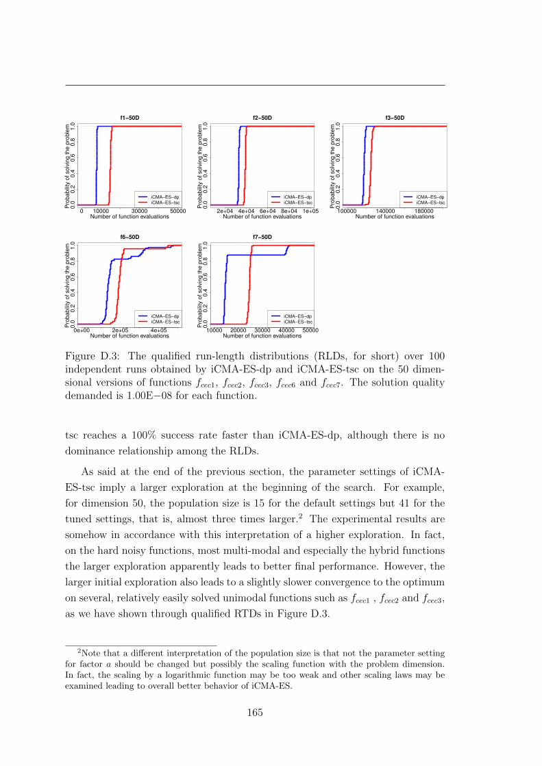
0 10000 30000 50000
0.0
0.2
0.4
0.6
0.8
1.0
Number of function evaluations
Pro
ba
bili
ty o
f so
lvin
g t
he
pro
ble
m
iCMA−ES−dp
iCMA−ES−tsc
f1−50D
2e+04 4e+04 6e+04 8e+04 1e+05
0.0
0.2
0.4
0.6
0.8
1.0
Number of function evaluations
Pro
ba
bili
ty o
f so
lvin
g t
he
pro
ble
m
iCMA−ES−dp
iCMA−ES−tsc
f2−50D
100000 140000 180000
0.0
0.2
0.4
0.6
0.8
1.0
Number of function evaluations
Pro
ba
bili
ty o
f so
lvin
g t
he
pro
ble
m
iCMA−ES−dp
iCMA−ES−tsc
f3−50D
0e+00 2e+05 4e+05
0.0
0.2
0.4
0.6
0.8
1.0
Number of function evaluations
Pro
ba
bili
ty o
f so
lvin
g t
he
pro
ble
m
iCMA−ES−dp
iCMA−ES−tsc
f6−50D
10000 20000 30000 40000 50000
0.0
0.2
0.4
0.6
0.8
1.0
Number of function evaluations
Pro
ba
bili
ty o
f so
lvin
g t
he
pro
ble
m
iCMA−ES−dp
iCMA−ES−tsc
f7−50D
Figure D.3: The qualified run-length distributions (RLDs, for short) over 100independent runs obtained by iCMA-ES-dp and iCMA-ES-tsc on the 50 dimen-sional versions of functions fcec1, fcec2, fcec3, fcec6 and fcec7. The solution qualitydemanded is 1.00E−08 for each function.
tsc reaches a 100% success rate faster than iCMA-ES-dp, although there is no
dominance relationship among the RLDs.
As said at the end of the previous section, the parameter settings of iCMA-
ES-tsc imply a larger exploration at the beginning of the search. For example,
for dimension 50, the population size is 15 for the default settings but 41 for the
tuned settings, that is, almost three times larger.2 The experimental results are
somehow in accordance with this interpretation of a higher exploration. In fact,
on the hard noisy functions, most multi-modal and especially the hybrid functions
the larger exploration apparently leads to better final performance. However, the
larger initial exploration also leads to a slightly slower convergence to the optimum
on several, relatively easily solved unimodal functions such as fcec1 , fcec2 and fcec3,
as we have shown through qualified RTDs in Figure D.3.
2Note that a different interpretation of the population size is that not the parameter settingfor factor a should be changed but possibly the scaling function with the problem dimension.In fact, the scaling by a logarithmic function may be too weak and other scaling laws may beexamined leading to overall better behavior of iCMA-ES.
165

D. COMPUTATIONAL RESULTS FOR AN AUTOMATICALLY TUNEDIPOP-CMA-ES ON THE CEC’05 BENCHMARK SET
1e−08 1e−05 1e−02 1e+01 1e+04
1e−
08
1e−
05
1e−
02
1e+
01
1e+
04
iCMA−ES−tsc (opt 9 )
Se
p−
iCM
A−
ES
−ts
c (
op
t 4
)
f_id_opt
3
6
7
8
9
10
11
12
1314
151617
1819202122232425
−Win 16 +
−Lose 5
−Draw 4
Average Errors−10D
100 500
100
200
500
15
16
17 16
25
2122
231819 20
1e−08 1e−05 1e−02 1e+01 1e+04
1e−
08
1e−
05
1e−
02
1e+
01
1e+
04
iCMA−ES−tsc (opt 7 )S
ep
−iC
MA
−E
S−
tsc (
op
t 3
)
f_id_opt
3
45
6
8
910
11
12
1314
1516
17181920212223
2425
−Win 16 +
−Lose 3
−Draw 6
Average Errors−30D
0.5 5.0 50.0
0.5
10.0
8
910
13
14
16
190 210 230
190
220 15
24
25
400 600 900
400
800
21 2322
18,19,20
1e−08 1e−05 1e−02 1e+01 1e+04
1e−
08
1e−
05
1e−
02
1e+
01
1e+
04
iCMA−ES−tsc (opt 7 )
Se
p−
iCM
A−
ES
−ts
c (
op
t 3
)
f_id_opt
3
45
6
8
91011
12
1314
1516
17181920212223
2425
−Win 18 +
−Lose 3
−Draw 4
Average Errors−50D
1 5 20 100
110
200
91013
8 1416
17
190 210 230
190
220
15
24
25
650 800 950
860
940
21
22
23
18,19,20
Figure D.4: Correlation plots of iCMA-ES-tsc and Sep-iCMA-ES-tsc on dimen-sions 10, 30 and 50 respectively. Each point represents the mean error value over 25independent runs obtained by either of the two algorithms. A point on the uppertriangle delimited by the diagonal indicates better performance for the algorithmon the x-axis; a point on the lower right triangle indicates better performance forthe algorithm on the y-axis. The number labeled beside some outstanding pointsrepresent the index of the corresponding function. The comparison is conductedbased on mean error values and the comparison results of the algorithm on thex-axis are presented in the form of -win, -draw, -lose, respectively, using iCMA-ES-tsc as the reference. We marked with a + symbol those cases in which thereis a statistically significant difference at the 0.05 α-level between the algorithms.The number of opt on the axes shows the number of means that is lower than thezero threshold, obtained by the corresponding algorithm.
D.4.2 iCMA-ES-tsc vs. iCMA-ES-tcec
One may wonder whether tuning iCMA-ES on the CEC’05 benchmark suite di-
rectly incurs better final performance on this set of functions. To explore this ques-
tion, we compare in Table D.4 the performance of iCMA-ES-tcec and iCMA-ES-tsc
on the CEC’05 benchmark set. iCMA-ES-tcec and iCMA-ES-tsc are mutually sta-
tistically better than each other on four functions of dimension 10, respectively. On
the 10 dimensional functions, iCMA-ES-tsc is slightly worse than iCMA-ES-tcec
with respect to the distribution of mean or median errors. This may be due to the
fact that iCMA-ES-tcec is tuned on the 10 dimensional CEC’05 benchmark set, the
same functions on which it is tested. Interestingly, this slight superiority of iCMA-
ES-tcec on the 10 dimensional functions does not generalize to higher dimensions.
As an example, consider functions fcec18, fcec19, fcec20 of dimension 10. On these,
iCMA-ES-tcec obtains an error value of 3.00E+02 in all independent 25 runs which
is the lowest value reported in the literature for these functions as far as we aware.
However, on the 50 dimensional version of these functions, iCMA-ES-tcec is sig-
166

nificantly worse than iCMA-ES-tsc. Moreover, considering the differences on all
functions of dimension 50, iCMA-ES-tsc statistically significantly improves upon
iCMA-ES-tcec on 12 functions while it performs statistically significantly worse
than iCMA-ES-tcec on only 3 functions. Considering the distribution of the mean
or median error values of the 50 dimensional functions, iCMA-ES-tsc statistically
significantly improves upon iCMA-ES-tcec.
It should also be mentioned that tuning on the SOCO benchmark functions
is much faster than on the CEC’05 benchmark set. In fact, the difference in
computation time amounts to a factor of about 50. This difference is mainly due to
the fact that 16 of the 25 CEC’05 functions of each dimension are rotated functions,
which requires more costly computations in the evaluation such as multiplication
operations on a rotated matrix.
D.4.3 Comparison to state-of-the-art methods that exploit
CMA-ES
At least two recent, newly designed state-of-the-art algorithms exploit CMA-ES
as an underlying local search method; these are a memetic algorithm with local
search chains based on CMA-ES (MA-LSch-CMA) [Molina et al., 2010a] and a
hybridization of a PSO algorithm with CMA-ES (PS-CMA-ES) [Muller et al.,
2009]. We compare iCMA-ES-tsc to these following the experimental analysis used
in Molina et al. [2010a] and Muller et al. [2009], that is by (i) statistically analyzing
for the distribution of the mean errors as in Molina et al. [2010a] and, (ii) ranking
the mean errors as in Muller et al. [2009]. As the results of MA-LSch-CMA and PS-
CMA-ES we use those reported in Liao et al. [2011a]. Note that the original results
reported in Molina et al. [2010a], Muller et al. [2009] did not necessarily satisfy
the bound constraints of the CEC’05 benchmark functions, which is corrected in
the results reported in [Liao et al., 2011a]. Table D.5 shows that iCMA-ES-tsc
performs statistically significantly better than MA-LSch-CMA in all dimensions;
iCMA-ES-tsc performs statistically significantly better than PS-CMA-ES on the
50 dimensional functions and it reaches better performance than PS-CMA-ES on
more functions for dimensions 10 and 30. Table D.5 also shows that iCMA-ES-
tsc obtains the best average ranking in all dimensions and most often the zero
threshold in all dimensions. Clearly, it would be interesting to also automatically
tune MA-LSch-CMA and PS-CMA-ES to exploit possibly more their potential.
Nevertheless, this comparison indicates that a feasible way to go for improving
the performance of iCMA-ES-dp is to further fine-tune iCMA-ES parameters (or
167

D. COMPUTATIONAL RESULTS FOR AN AUTOMATICALLY TUNEDIPOP-CMA-ES ON THE CEC’05 BENCHMARK SET
maybe other design choices of iCMA-ES) instead of embedding CMA-ES into other
algorithms. Recall that this also justifies the effort in tuning iCMA-ES because
when designing new hybrid algorithms, often also a substantially large effort flows
into the further, often manual fine-tuning of algorithm parameters and algorithm
designs.
D.5 Additional experiments
D.5.1 Comparison to other results by iCMA-ES
We also compared iCMA-ES-tsc to Sep-iCMA-ES-tsc [Liao et al., 2011c], the
algorithm used by Smit and Eiben [2010], on the full CEC’05 benchmark set.
Fig. D.4 shows correlation plots that illustrate the relative performance for
Sep-iCMA-ES-tsc and iCMA-ES-tsc on dimensions 10, 30 and 50, respectively.
Each point represents the mean error value obtained by either of the two al-
gorithms. These plots indicate superior performance of iCMA-ES-tsc over Sep-
iCMA-ES-tsc, which is confirmed by the table of full results available at http:
//iridia.ulb.ac.be/supp/IridiaSupp2011-023. We verified that iCMA-ES-
tsc reaches statistically significantly better performance than Sep-iCMA-ES-tsc
on the distribution of mean error values on all dimensions. This comparison con-
firms our expectation of iCMA-ES-tsc’s superiority over Sep-iCMA-ES-tsc on the
CEC’05 benchmark set, where 16 of 25 functions are rotated functions. The most
significant example is fcec3, a unimodal rotated high conditional function, where
Sep-iCMA-ES-tsc stagnated at very high mean error values for all dimensions,
while iCMA-ES-tsc reached in each trial the zero threshold. However, Sep-iCMA-
ES-tsc obtains better performance than iCMA-ES-tsc on fcec10, a rotated Rastrigin
function, over all dimensions. This case gives an indication that we can only con-
clude that iCMA-ES’s rotational invariance plays a pivotal role to handle most
but not all rotated functions.
Next, we take the mean errors reported for iCMA-ES in the CEC’05 special
session as a reference and refer to these results as iCMA-ES-05. Note that the
results of iCMA-ES-05 were obtained with a different implementation (using the
Matlab and not the C code we use) and with a much more sophisticated bound
handling mechanism. We summarize the comparison with iCMA-ES-tsc in Table
D.6. iCMA-ES-tsc performs statistically significantly better than iCMA-ES-05 on
dimension 30 and it reaches on more functions statistically significantly better
results (on a per function basis). This confirms the high performance of iCMA-
168

ES-tsc.
D.5.2 Tuning setup
In this section, we examine different choices for the composition of the training set
to obtain an indication which types of functions are important for high performance
of the tuned iCMA-ES. We also explore alternative settings of the irace tool.
In what follows, we define training sets that are composed of different subsets of
the SOCO benchmark functions and evaluate the tuned performance of iCMA-ES
using the mean errors on the 50-dimensional CEC’05 benchmark functions. We
summarize here our main findings and for detailed numerical results we refer to
the supplementary page http://iridia.ulb.ac.be/supp/IridiaSupp2011-023.
The convention we use for labeling the training function sets is introduced first:
⊕ all hybrid functions of SOCO
uni uni-modal functions of SOCO except fsoco1, fsoco8
multi all non-hybrid multi modal functions of SOCO
except fsoco3, fsoco4
+ adds the uni-modal (fsoco1, fsoco8) or multi modal
(fsoco3,fsoco4) functions to respective training sets
For example, iCMA-ES-⊕ denotes iCMA-ES tuned using only the eight hybrid
functions, iCMA-ES-uni,multi denotes iCMA-ES tuned with the seven uni-modal
and (non-hybrid) multi-modal functions of SOCO, and iCMA-ES-uni+ denotes
iCMA-ES tuned with all seven uni-modal functions.
In Table D.7 we summarize the average ranking and the statistical analysis
of several parameter settings of iCMA-ES that were obtained with the various
training set compositions that we considered. In Table D.8 are given the parameter
setting obtained using these training set compositions; the parameter settings for
iCMA-ES-tsc and iCMA-ES-dp are given in Table D.1. The main conclusions we
can obtain are the following.
1. The usage of the hybrid functions in the training set is a key to high tuned
performance. iCMA-ES-⊕ obtains about the same performance as iCMA-
ES-tsc and if the hybrid functions are not part of the training set, the per-
formance of the tuned iCMA-ES degrades considerably. Interestingly, the
configuration iCMA-ES-⊕ obtains on all 50-dimensional hybrid functions of
CEC’05 significantly better results than iCMA-ES-tsc-uni,multi, indicating
169
D. COMPUTATIONAL RESULTS FOR AN AUTOMATICALLY TUNEDIPOP-CMA-ES ON THE CEC’05 BENCHMARK SET
that there are maybe some common aspects between the hybrid functions of
the SOCO and the CEC’05 benchmark set.
2. The usage of the multi-modal functions only, that is, configuration iCMA-
ES-multi, leads to significantly worse performance than iCMA-ES-⊕. One
may object that the set multi contains only two training functions; however,
adding the two multi-modal functions fsoco3 and fsoco4 to the training set does
not lead to much improved performance (configuration iCMA-ES-multi+, see
http://iridia.ulb.ac.be/supp/IridiaSupp2011-023).
3. Configuration iCMA-ES-uni leads to, at first sight, surprisingly high per-
formance on the CEC’05 functions, and it has only a slightly worse mean
rank than iCMA-ES-⊕. At a second glance, it is noteworthy that uni-modal
functions such as those in the set “uni” can actually be quite difficult to
optimize; for example, the default parameter setting of iCMA-ES has poor
performance on uni-modal functions fcec4 and fcec5 (see Table D.3). Config-
urations iCMA-ES-uni+, which uses also functions fsoco1 and fsoco8 in the
training set, is, however, worse than iCMA-ES-uni (and significantly worse
performing than iCMA-ES-⊕). This is possibly caused by floor effects ob-
tained due to adding functions that are easily solved by iCMA-ES.
A common pattern among the best performing parameter settings, which are
iCMA-ES-tsc, iCMA-ES-⊕, and iCMA-ES-uni, is that they tend to increase the
exploration performed by iCMA-ES. In fact, the commonalities of these parameter
settings are a higher population size, a (slightly) larger initial step size, and a faster
increase of the population size upon a restart than the default parameter settings.
Since these parameter settings improve performance, in particular, on the hardest
benchmark problems, it may be that the default settings were possibly biased by
experiments on too simple benchmark functions.
Considering the tuning setup, we also made tests (i) replacing the F-test with a
t-test (that is, using the Student t-test for the race) and (ii) increasing the tuning
budget to 25000 runs. Similar to the results reported previously by iCMA-ES-tsc,
the resulting configurations improved upon iCMA-ES-dp, being statistically sig-
nificantly better than iCMA-ES-dp on the distribution of the mean or the median
error values. These experiments also indicate that the observation of the superior
performance of iCMA-ES-tsc over iCMA-ES-dp is relatively stable with respect to
some (minor) changes in the tuning setup. The detailed data of these trials are
available at http://iridia.ulb.ac.be/supp/IridiaSupp2011-023.
170

D.6 Conclusions and future work
In this chapter, we tuned iCMA-ES to improve its performance on the CEC’05
benchmark set. We did so by using a separation between training and test set
to avoid the bias of the results due to potentially overtuning the algorithm. Our
experimental results showed that the tuned iCMA-ES improves significantly over
the default parameter settings of iCMA-ES-dp. While on some individual func-
tions the improvements observed from a solution quality perspective are rather
large, on many other functions only minor though often statistically significant
improvements are observed. iCMA-ES-tsc also performs competitive or superior to
methods, such as MA-LSch-CMA [Molina et al., 2010a] and PS-CMA-ES [Muller
et al., 2009], which were developed with the goal of improving over iCMA-ES
performance. This indicates that, instead of embedding CMA-ES into other algo-
rithms to improve over its performance, a viable, alternative approach is to further
fine-tune the parameter settings or maybe some design choices of iCMA-ES. This
direction would involve to further parameterize choices that are currently fixed in
the algorithm. Examples of such parameterizations are to treat further constants
as parameters that are to be tuned or to consider alternative choices for specific
functions. A concrete example could be the formula that is used to determine
the initial population size, which is 4 + ba ln(D)c (see also Table D.1). Here, the
constant 4 could be replaced by a real-valued parameter and different functions
(instead of + and ln may be considered.
It is also interesting to consider the impact the tuned parameter settings have
on the behavior of iCMA-ES. In fact, a common pattern among the best performing
tuned parameter settings we observed is that they lead to an increased exploration
of the search space at least in the initial search phases and upon a restart of
iCMA-ES. This more explorative behavior is implied by larger population sizes,
larger step sizes, and a higher factor for the increase of the population size upon
a restart of iCMA-ES. Interestingly, increasing search space exploration is also
often the goal of hybrid algorithms such as the above mentioned MA-LSch-CMA
and PS-CMA-ES where CMA-ES is used as a local search. In fact, it seems that
such increased exploration can directly provided inside the iCMA-ES framework
by modified parameter settings.
Our experimental results also indicate that using off-line automatic algorithm
configuration to further improve adaptive algorithms is a viable approach—recall
that iCMA-ES is such an adaptive algorithm where step sizes and search directions
are adapted to the particular continuous optimization function under concern.
171

D. COMPUTATIONAL RESULTS FOR AN AUTOMATICALLY TUNEDIPOP-CMA-ES ON THE CEC’05 BENCHMARK SET
We have also presented initial results examining the role of the specific com-
position of a training set on the performance of the tuned parameter settings.
On the one hand, these results indicated that the hybrid functions in the SOCO
benchmark set alone are enough to derive high-performing tuned parameter set-
tings. Maybe surprisingly, using only the uni-modal functions of the SOCO
benchmark set resulted in a same level of performance of the tuned iCMA-ES
on the CEC’05 benchmark set. Although it is known that uni-modal functions
can be difficult to optimize, in future research the importance of the training
set should be examined in much more detail. For this task, it is important to
consider interactions between algorithm properties and properties of the train-
ing set. For example, the fact that iCMA-ES is rotationally invariant made it
possible to use the SOCO benchmark set of functions which contains only unro-
tated functions—the rotational invariance implies that iCMA-ES’s performance
should be unaffected by rotations of the functions. For algorithms that are not
invariant with respect to rotations, the usage of the SOCO benchmark set as
training set may actually lead to poor performance. An interesting direction
here would be to consider other benchmark set such as the BBOB benchmark
function suite (see http://coco.gforge.inria.fr/doku.php?id=bbob-2012) or
newly designed benchmark suites containing functions with specific properties for
the tuning of continuous optimizers.
172

Tab
leD
.3:
Res
ult
sof
the
com
par
ison
bet
wee
niC
MA
-ES-d
pan
diC
MA
-ES-t
scov
er25
indep
enden
tru
ns
for
CE
C’0
5fu
nct
ions.
Sym
bol
s<
,≈
,an
d>
den
ote
whet
her
the
per
form
ance
ofiC
MA
-ES-d
pis
stat
isti
call
yb
ette
r,in
diff
eren
t,or
wor
seth
anth
atof
iCM
A-E
S-t
scac
cord
ing
toth
etw
o-si
ded
Wilco
xon
mat
ched
-pai
rssi
gned
-ran
kte
stat
the
0.05
α-l
evel
.T
he
num
ber
sin
par
enth
esis
repre
sent
the
tim
esof<
,≈
,an
d>
,re
spec
tive
ly.
The
num
ber
sin
par
enth
esis
for
(<,
=,>
)re
pre
sent
the
tim
esw
ehav
e<
,=
,an
d>
,re
spec
tive
ly,
when
iCM
A-E
S-d
pis
com
par
edw
ith
iCM
A-E
S-t
scbas
edon
the
mea
nor
med
ian
erro
rs.
f cec
10
dim
ensi
ons
30dim
ensi
ons
50
dim
ensi
ons
iCM
A-E
S-d
piC
MA
-ES-t
sciC
MA
-ES-d
piC
MA
-ES-t
sciC
MA
-ES-d
piC
MA
-ES-t
scM
ean
and
Med
ian
Mea
nan
dM
edia
nM
ean
and
Med
ian
Mea
nan
dM
edia
nM
ean
and
Med
ian
Mea
nan
dM
edia
nf 1
1.0
0E−
08
1.00
E−
08≈
1.00
E−
08
1.0
0E−
08
1.0
0E−
08
1.0
0E−
08≈
1.0
0E−
08
1.00
E−
08
1.00E−
08
1.0
0E−
08≈
1.0
0E−
081.
00E−
08
f 21.0
0E−
08
1.00
E−
08≈
1.00
E−
08
1.0
0E−
08
1.0
0E−
08
1.0
0E−
08≈
1.0
0E−
08
1.00
E−
08
1.00E−
08
1.0
0E−
08≈
1.0
0E−
081.
00E−
08
f 31.0
0E−
08
1.00
E−
08≈
1.00
E−
08
1.0
0E−
08
1.0
0E−
08
1.0
0E−
08≈
1.0
0E−
08
1.00
E−
08
1.00E−
08
1.0
0E−
08≈
1.0
0E−
081.
00E−
08
f 41.0
0E−
08
1.00
E−
08≈
1.00
E−
08
1.0
0E−
08
6.5
8E
+02
1.7
5E
+00>
1.0
0E−
08
1.00
E−
08
1.43E
+04
1.2
7E
+04>
1.0
0E−
081.
00E−
08
f 51.0
0E−
08
1.00
E−
08≈
1.00
E−
08
1.0
0E−
08
1.0
0E−
08
1.0
0E−
08≈
1.0
0E−
08
1.00
E−
08
7.41E−
02
8.6
1E−
08>
1.0
0E−
081.
00E−
08
f 61.0
0E−
08
1.00
E−
08≈
1.00
E−
08
1.0
0E−
08
1.0
0E−
08
1.0
0E−
08≈
1.0
0E−
08
1.00
E−
08
1.00E−
08
1.0
0E−
08≈
1.0
0E−
081.
00E−
08
f 71.0
0E−
08
1.00
E−
08≈
1.00
E−
08
1.0
0E−
08
1.0
0E−
08
1.0
0E−
08≈
1.0
0E−
08
1.00
E−
08
1.00E−
08
1.0
0E−
08≈
1.0
0E−
081.
00E−
08
f 82.0
0E+
012.
00E
+01≈
2.02
E+
01
2.00
E+
01
2.0
4E
+01
2.0
0E
+01<
2.0
8E
+01
2.10E
+01
2.09E
+01
2.1
1E
+01≈
2.1
0E
+01
2.11E
+01
f 91.5
9E−
01
1.00
E−
08≈
4.81
E−
02
1.0
0E−
08
1.8
7E
+00
1.9
9E
+00≈
1.9
9E
+00
1.99E
+00
4.36E
+00
3.9
8E
+00≈
4.1
8E
+00
3.98E
+00
f 10
3.1
8E−
01
1.00
E−
08≈
3.73
E−
03
1.0
0E−
08
1.4
4E
+00
9.9
5E−
01≈
1.5
9E
+00
9.95E−
01
2.89E
+00
1.9
9E
+00≈
2.7
1E
+00
2.98E
+00
f 11
1.0
0E−
08
1.00
E−
08≈
1.00
E−
08
1.0
0E−
08
7.1
7E−
02
1.0
0E−
08>
5.0
9E−
05
1.00
E−
08
9.94E−
02
1.0
0E−
08≈
6.0
3E−
021.
00E−
08
f 12
4.0
7E+
031.
00E−
08>
1.00
E−
08
1.0
0E−
08
1.1
9E
+04
4.8
4E
+03>
4.2
2E
+02
5.96E
+01
4.25E
+04
2.7
8E
+04>
4.6
9E
+03
3.39E
+03
f 13
6.4
9E−
01
6.37
E−
01≈
7.14
E−
01
6.9
4E−
01
2.6
3E
+00
2.7
1E
+00≈
2.5
3E
+00
2.57E
+00
4.44E
+00
4.3
7E
+00<
4.7
0E
+00
4.62E
+00
f 14
1.9
6E+
001.
98E
+00≈
2.03
E+
00
2.09
E+
00
1.2
6E
+01
1.2
6E
+01>
1.1
0E
+01
1.13E
+01
2.28E
+01
2.3
0E
+01>
2.0
9E
+01
2.12E
+01
f 15
2.1
5E+
022.
00E
+02<
3.32
E+
02
4.00
E+
02
2.0
0E
+02
2.0
0E
+02≈
2.0
0E
+02
2.00E
+02
2.00E
+02
2.0
0E
+02≈
2.0
0E
+02
2.00E
+02
f 16
9.0
4E+
019.
11E
+01>
8.86
E+
01
9.03
E+
01
1.4
8E
+01
1.5
1E
+01>
1.1
1E
+01
1.07E
+01
1.10E
+01
1.1
4E
+01>
5.3
4E
+00
5.47E
+00
f 17
1.1
7E+
021.
09E
+02>
9.34
E+
01
9.43
E+
01
2.5
2E
+02
1.8
0E
+02>
2.0
8E
+02
5.60E
+01
1.91E
+02
1.6
2E
+02>
6.3
6E
+01
4.99E
+01
f 18
3.1
6E+
023.
00E
+02<
3.60
E+
02
3.00
E+
02
9.0
4E
+02
9.0
4E
+02≈
9.0
4E
+02
9.04E
+02
9.13E
+02
9.1
6E
+02>
9.1
3E
+02
9.13E
+02
f 19
3.2
0E+
023.
00E
+02≈
3.20
E+
02
3.00
E+
02
9.0
4E
+02
9.0
4E
+02≈
9.0
4E
+02
9.04E
+02
9.13E
+02
9.1
5E
+02>
9.1
3E
+02
9.13E
+02
f 20
3.2
0E+
023.
00E
+02≈
3.40
E+
02
3.00
E+
02
9.0
4E
+02
9.0
4E
+02≈
9.0
4E
+02
9.04E
+02
9.15E
+02
9.1
5E
+02>
9.1
3E
+02
9.13E
+02
f 21
5.0
0E+
025.
00E
+02≈
5.00
E+
02
5.00
E+
02
5.0
0E
+02
5.0
0E
+02≈
5.0
0E
+02
5.00E
+02
6.64E
+02
5.0
0E
+02≈
7.0
5E
+02
5.00E
+02
f 22
7.2
8E+
027.
28E
+02≈
7.28
E+
02
7.28
E+
02
8.1
0E
+02
8.1
1E
+02≈
8.1
7E
+02
8.24E
+02
8.19E
+02
8.1
8E
+02≈
8.1
9E
+02
8.21E
+02
f 23
5.8
6E+
025.
59E
+02≈
5.59
E+
02
5.59
E+
02
5.3
4E
+02
5.3
4E
+02≈
5.3
4E
+02
5.34E
+02
6.97E
+02
5.4
0E
+02≈
7.3
0E
+02
5.40E
+02
f 24
2.3
3E+
022.
00E
+02≈
2.00
E+
02
2.00
E+
02
2.0
0E
+02
2.0
0E
+02≈
2.0
0E
+02
2.00E
+02
2.00E
+02
2.0
0E
+02≈
2.0
0E
+02
2.00E
+02
f 25
4.3
4E+
024.
04E
+02>
4.03
E+
02
4.03
E+
02
2.1
0E
+02
2.1
0E
+02>
2.0
9E
+02
2.09E
+02
2.14E
+02
2.1
4E
+02>
2.1
3E
+02
2.13E
+02
Mea
nf 1
-f25
(<,
=,>
):(6
,11
,8)
f 1-f
25(<
,=
,>
):(4
,13
,8)
f 1-f
25(<
,=
,>
):(4
,10,
11)†
Med
ian
f 1-f
25
(<,
=,>
):(3
,19
,3)
f 1-f
25(<
,=
,>
):(2
,16
,7)
f 1-f
25(<
,=
,>
):(3
,12,
10)†
By
Func
f 1-f
25
(<,≈
,>
):(2
,19
,4)
f 1-f
25(<
,≈
,>
):(1
,17
,7)
f 1-f
25(<
,≈
,>
):(1
,14,
10)
10,
30
and
50
dim
ensi
onalf 1
-f25
(<,>
):(5
%,
28%
)†
den
ote
sth
ere
isa
sign
ifica
nt
diff
eren
ceov
erth
edis
trib
uti
on
of
mea
nor
med
ian
erro
rsb
etw
een
iCM
A-E
S-d
pw
ith
iCM
A-E
S-t
scby
atw
o-si
ded
Wilco
xon
mat
ched
-pai
rssi
gned
-ran
ks
test
atth
e0,0
5α
-lev
el.
173

D. COMPUTATIONAL RESULTS FOR AN AUTOMATICALLY TUNEDIPOP-CMA-ES ON THE CEC’05 BENCHMARK SET
Tab
leD
.4:C
omp
arisonb
etween
iCM
A-E
S-tcec
and
iCM
A-E
S-tsc
over25
indep
end
ent
runs
forC
EC
’05fu
nction
s.Sym
bols
<,≈
,an
d>
den
otew
heth
erth
ep
erforman
ceof
iCM
A-E
S-tcec
isstatistically
better,
indiff
erent,
orw
orseth
anth
atof
iCM
A-
ES
-tscaccord
ing
toth
etw
o-sided
Wilcox
onm
atched
-pairs
signed
-rank
testat
the
0.05α
-level.T
he
num
bers
inparen
thesis
represen
tth
etim
esof<
,≈,
and>
,resp
ectively.T
he
num
bers
inparen
thesis
for(<
,=
,>
)rep
resent
the
times
we
have
<,
=,
and>
,resp
ectively,w
hen
iCM
A-E
S-d
pis
compared
with
iCM
A-E
S-tsc
based
onth
em
eanor
med
ianerrors.
fcec
10dim
ension
s30
dim
ension
s50
dim
ension
siC
MA
-ES-tcec
iCM
A-E
S-tsc
iCM
A-E
S-tcec
iCM
A-E
S-tsc
iCM
A-E
S-tcec
iCM
A-E
S-tsc
Mean
and
Med
ianM
eanand
Med
ian
Mean
and
Med
ian
Mea
nan
dM
edian
Mean
and
Med
ian
Mea
nan
dM
edian
f1
1.00E−
081.0
0E−08≈
1.00E−08
1.0
0E−
08
1.00E−
08
1.00
E−08≈
1.00
E−08
1.00E−
08
1.00
E−08
1.00E−
08≈
1.00
E−08
1.00E−
08f2
1.00E−
081.0
0E−08≈
1.00E−08
1.0
0E−
08
1.00E−
08
1.00
E−08≈
1.00
E−08
1.00E−
08
1.00
E−08
1.00E−
08≈
1.00
E−08
1.00E−
08f3
1.00E−
081.0
0E−08≈
1.00E−08
1.0
0E−
08
1.00E−
08
1.00
E−08≈
1.00
E−08
1.00E−
08
1.00
E−08
1.00E−
08≈
1.00
E−08
1.00E−
08f4
1.00E−
081.0
0E−08≈
1.00E−08
1.0
0E−
08
1.00E−
08
1.00
E−08≈
1.00
E−08
1.00E−
08
2.85
E+
021.0
0E−08>
1.00
E−08
1.00E−
08f5
1.00E−
081.0
0E−08≈
1.00E−08
1.0
0E−
08
2.69E−
08
2.72
E−08>
1.00
E−08
1.00E−
08
5.02
E−08
4.85E−
08>
1.00
E−08
1.00E−
08f6
1.00E−
081.0
0E−08≈
1.00E−08
1.0
0E−
08
2.79E−
02
1.00
E−08≈
1.00
E−08
1.00E−
08
1.00
E−08
1.00E−
08≈
1.00
E−08
1.00E−
08f7
1.00E−
081.0
0E−08≈
1.00E−08
1.0
0E−
08
1.00E−
08
1.00
E−08≈
1.00
E−08
1.00E−
08
1.00
E−08
1.00E−
08≈
1.00
E−08
1.00E−
08f8
2.01E
+01
2.00E
+01≈
2.02E+
012.0
0E
+01
2.08E
+01
2.09
E+
01≈
2.08
E+
012.1
0E+
01
2.08
E+
012.1
1E+
01<
2.10
E+
012.1
1E+
01
f9
2.64E−
011.0
0E−08>
4.81E−02
1.0
0E−
08
2.15E
+00
1.99
E+
00≈
1.99
E+
001.9
9E+
00
5.49
E+
005.9
7E+
00>
4.18
E+
003.9
8E+
00
f10
1.59E−
011.0
0E−08>
3.73E−03
1.0
0E−
08
1.67E
+00
1.99
E+
00>
1.59
E+
009.9
5E−01
3.54
E+
003.9
8E+
00>
2.71
E+
002.9
8E+
00
f11
1.00E−
081.0
0E−08≈
1.00E−08
1.0
0E−
08
8.69E−
02
1.00
E−08>
5.09
E−05
1.00E−
08
1.83
E−01
1.00E−
08≈
6.03
E−02
1.00E−
08f12
1.00E−
081.0
0E−08≈
1.00E−08
1.0
0E−
08
4.88E
+02
1.92
E+
02≈
4.22
E+
025.9
6E+
01
6.41
E+
034.5
9E+
03≈
4.69
E+
033.3
9E+
03
f13
6.14E−
016.4
6E−01<
7.14E−01
6.9
4E−
01
2.48E
+00
2.50
E+
00≈
2.53
E+
002.5
7E+
00
4.42
E+
004.4
7E+
00<
4.70
E+
004.6
2E+
00
f14
8.07E−
016.6
6E−01<
2.03E+
002.0
9E
+00
9.93E
+00
9.94
E+
00<
1.10
E+
011.1
3E+
01
2.02
E+
011.9
8E+
01<
2.09
E+
012.1
2E+
01
f15
2.96E
+02
3.00E
+02<
3.32E+
024.0
0E
+02
2.00E
+02
2.00
E+
02≈
2.00
E+
022.0
0E+
02
2.00
E+
022.0
0E+
02≈
2.00
E+
022.0
0E+
02
f16
8.83E
+01
8.94E
+01≈
8.86E+
019.0
3E
+01
1.06E
+01
1.04
E+
01≈
1.11
E+
011.0
7E+
01
9.46
E+
009.0
9E+
00>
5.34
E+
005.4
7E+
00
f17
1.20E
+02
1.17E
+02>
9.34E+
019.4
3E
+01
2.14E
+02
1.52
E+
02≈
2.08
E+
025.6
0E+
01
9.55
E+
018.0
6E+
01>
6.36
E+
014.9
9E+
01
f18
3.00E
+02
3.00E
+02<
3.60E+
023.0
0E
+02
9.04E
+02
9.04
E+
02≈
9.04
E+
029.0
4E+
02
9.15
E+
029.1
6E+
02>
9.13
E+
029.1
3E+
02
f19
3.00E
+02
3.00E
+02≈
3.20E+
023.0
0E
+02
9.04E
+02
9.04
E+
02≈
9.04
E+
029.0
4E+
02
9.16
E+
029.1
6E+
02>
9.13
E+
029.1
3E+
02
f20
3.00E
+02
3.00E
+02≈
3.40E+
023.0
0E
+02
9.04E
+02
9.04
E+
02≈
9.04
E+
029.0
4E+
02
9.15
E+
029.1
4E+
02>
9.13
E+
029.1
3E+
02
f21
5.00E
+02
5.00E
+02≈
5.00E+
025.0
0E
+02
5.00E
+02
5.00
E+
02≈
5.00
E+
025.0
0E+
02
9.68
E+
021.0
1E+
03>
7.05
E+
025.0
0E+
02
f22
7.27E
+02
7.26E
+02≈
7.28E+
027.2
8E
+02
8.10E
+02
8.07
E+
02≈
8.17
E+
028.2
4E+
02
8.15
E+
028.1
4E+
02≈
8.19
E+
028.2
1E+
02
f23
5.59E
+02
5.59E
+02≈
5.59E+
025.5
9E
+02
5.34E
+02
5.34
E+
02≈
5.34
E+
025.3
4E+
02
9.04
E+
021.0
2E+
03>
7.30
E+
025.4
0E+
02
f24
2.00E
+02
2.00E
+02≈
2.00E+
022.0
0E
+02
2.00E
+02
2.00
E+
02≈
2.00
E+
022.0
0E+
02
2.00
E+
022.0
0E+
02≈
2.00
E+
022.0
0E+
02
f25
4.04E
+02
4.04E
+02>
4.03E+
024.0
3E
+02
2.09E
+02
2.09
E+
02>
2.09
E+
022.0
9E+
02
2.13
E+
022.1
3E+
02>
2.13
E+
022.1
3E+
02
Mean
f1 -f
25
(<,
=,>
):(9,
12,
4)
f1 -f
25 (<
,=
,>
):(4,
14,
7)f1 -f
25 (<
,=
,>
):(4
,8,
14) †
Med
ianf1 -f
25
(<,
=,>
):(5,
18,
2)
f1 -f
25 (<
,=
,>
):(5,
16,
4)f1 -f
25 (<
,=
,>
):(3
,11
,11
) †
By
Func
f1 -f
25
(<,≈
,>
):(4,
17,
4)
f1 -f
25 (<
,≈,>
):(1,
20,
4)f1 -f
25 (<
,≈,>
):(3
,10,
12)
10,
30
and
50dim
ension
alf1 -f
25
(<,>
):(11%
,27
%)
†den
otes
there
isa
signifi
cant
diff
erence
overth
edistrib
ution
ofm
eanor
med
ian
errors
betw
eeniC
MA
-ES-tcec
with
iCM
A-E
S-tsc
by
atw
o-sid
edW
ilcoxon
match
ed-p
airssign
ed-ra
nks
testat
the
0,0
5α
-level.
174

Tab
leD
.5:
The
mea
ner
rors
obta
ined
by
MA
-LSch
-CM
A,
PS-C
MA
-ES
and
iCM
A-E
S-t
sc(M
A,
PS,
iCM
AE
St
for
thei
rab
bre
via
tion
s,re
spec
tive
ly,
inth
ista
ble
)ov
er25
indep
enden
tru
ns
for
CE
C’0
5fu
nct
ions.
The
num
ber
sin
par
enth
esis
repre
sent
the
tim
esof<
,=
,an
d>
,re
spec
tive
ly,
when
the
corr
esp
ondin
gal
gori
thm
sar
eco
mpar
edw
ith
iCM
A-E
S-t
scbas
edon
the
mea
ner
rors
.T
he
num
ber
ofm
eans
bel
owth
eze
ro-t
hre
shol
dfo
und
by
each
algo
rith
m(i
ndic
ated
by
“Opti
ma”
and
the
aver
age
rankin
gof
each
algo
rith
mar
eal
sogi
ven.
f cec
10d
imen
sion
s30
dim
ensi
ons
50
dim
ensi
on
sM
ean
Err
ors
Mea
nE
rror
sM
ean
Err
ors
MA
PS
iCM
AE
St
MA
PS
iCM
AE
St
MA
PS
iCM
AE
St
f 11.
00E−
081.
00E−
08
1.0
0E−
08
1.0
0E−
081.
00E−
081.0
0E−
08
1.0
0E−
081.0
0E−
081.0
0E−
08
f 21.
00E−
081.
00E−
08
1.0
0E−
08
1.0
0E−
081.
00E−
081.0
0E−
08
3.0
6E−
027.3
6E−
061.0
0E−
08
f 31.
00E−
081.
45E−
01
1.0
0E−
08
2.7
5E+
042.
96E
+04
1.0
0E−
08
3.2
1E+
049.1
0E+
041.0
0E−
08f 4
5.54
E−
031.
00E−
08
1.0
0E−
08
3.0
2E+
024.
56E
+03
1.0
0E−
08
3.2
3E+
032.1
7E+
041.0
0E−
08f 5
6.75
E−
071.
00E−
08
1.0
0E−
08
1.2
6E+
032.
52E
+01
1.0
0E−
08
2.6
9E+
031.7
9E+
031.0
0E−
08f 6
3.19
E−
011.
00E−
08
1.0
0E−
08
1.1
2E+
001.
15E
+01
1.0
0E−
08
4.1
0E+
002.9
1E+
011.0
0E−
08f 7
1.43
E−
011.
00E−
08
1.0
0E−
08
1.7
5E−
021.
00E−
081.0
0E−
08
5.4
0E−
031.0
0E−
081.0
0E−
08
f 82.
00E
+01
2.00
E+
012.0
2E+
012.0
0E+
012.
00E
+01
2.0
8E
+01
2.0
0E+
012.0
0E+
012.1
0E+
01f 9
1.00
E−
083.
98E−
02
4.8
1E−
02
1.0
0E−
088.
76E−
011.9
9E+
001.0
0E−
085.4
5E+
004.1
8E+
00f 1
02.
67E
+00
1.00
E−
08
3.7
3E−
03
2.2
5E+
015.
57E−
011.5
9E+
005.0
1E+
015.3
3E+
002.7
1E+
00f 1
12.
43E
+00
8.51
E−
01
1.0
0E−
08
2.1
5E+
017.
10E
+00
5.0
9E−
05
4.1
3E+
011.5
9E+
016.0
3E−
02f 1
21.
14E
+02
1.10
E+
001.0
0E−
08
1.6
7E+
038.
80E
+02
4.2
2E
+02
1.3
9E+
046.9
0E+
034.6
9E+
03f 1
35.
45E−
013.
67E−
01
7.1
4E−
01
2.0
3E+
002.
05E
+00
2.5
3E
+00
3.1
5E+
004.1
5E+
004.7
0E+
00f 1
42.
25E
+00
3.40
E+
002.0
3E+
001.2
5E+
011.
24E
+01
1.1
0E
+01
2.2
2E+
012.1
5E+
012.0
9E+
01f 1
52.
24E
+02
8.67
E+
013.3
2E+
023.0
0E+
021.
37E
+02
2.0
0E
+02
3.7
2E+
021.2
5E+
022.0
0E+
02f 1
69.
18E
+01
9.28
E+
018.8
6E+
011.2
6E+
021.
59E
+01
1.1
1E
+01
6.9
0E+
011.6
2E+
015.3
4E+
00f 1
71.
01E
+02
1.12
E+
029.3
4E+
011.8
3E+
029.
15E
+01
2.0
8E
+02
1.4
7E+
029.1
3E+
016.3
6E+
01f 1
88.
84E
+02
3.60
E+
023.6
0E+
028.9
8E+
029.
05E
+02
9.0
4E
+02
9.4
1E+
028.7
0E+
029.1
3E+
02f 1
98.
78E
+02
3.25
E+
023.2
0E+
029.0
1E+
028.
85E
+02
9.0
4E
+02
9.3
8E+
029.1
3E+
029.1
3E+
02f 2
08.
63E
+02
3.43
E+
023.4
0E+
028.9
6E+
029.
05E
+02
9.0
4E
+02
9.2
8E+
029.0
9E+
029.1
3E+
02f 2
17.
94E
+02
4.71
E+
025.0
0E+
025.1
2E+
025.
00E
+02
5.0
0E
+02
5.0
0E+
026.6
2E+
027.0
5E+
02f 2
27.
53E
+02
7.46
E+
027.2
8E+
028.8
0E+
028.
43E
+02
8.1
7E
+02
9.1
4E+
028.6
3E+
028.1
9E+
02f 2
38.
88E
+02
5.58
E+
025.5
9E+
025.3
4E+
025.
34E
+02
5.3
4E
+02
5.3
9E+
028.1
2E+
027.3
0E+
02f 2
42.
28E
+02
2.00
E+
022.0
0E+
022.0
0E+
022.
00E
+02
2.0
0E
+02
2.0
0E+
022.0
0E+
022.0
0E+
02f 2
54.
55E
+02
4.00
E+
024.0
3E+
022.1
4E+
022.
10E
+02
2.0
9E
+02
2.2
1E+
022.1
4E+
022.1
3E+
02V
.S.
(3,
4,18
)†(8
,8,
9)
(7,
4,14)†
(7,
6,12)
(5,
2,
18)†
(6,
4,15
)†
Op
tim
a4
79
33
72
27
Ran
k2.
521.
781.7
2.2
61.9
81.7
62.
422.
021.5
6†
den
otes
ther
eis
asi
gnifi
cant
diff
eren
ceov
erth
ed
istr
ibu
tion
ofm
ean
erro
rsb
etw
een
the
corr
esp
ond
ing
algo
rith
mw
ith
iCM
A-E
S-t
scby
atw
o-si
ded
Wil
coxon
matc
hed
-pai
rssi
gned
-ran
ks
test
atth
e0,
05α
-lev
el.
175

D. COMPUTATIONAL RESULTS FOR AN AUTOMATICALLY TUNEDIPOP-CMA-ES ON THE CEC’05 BENCHMARK SET
Table D.6: Summary of the comparison withiCMA-ES-tsc on 10, 30 and 50 dimensions with re-spect to mean error values: (better, equal, worse).Error values lower than 10−8 are approximated to10−8.
iCMA-ES-05 Sep-iCMA-ES-tscvs. iCMA-ES-tsc vs. iCMA-ES-tsc
10 Dim (6, 10, 9) (5, 4, 16)†
30 Dim (4, 11, 10)† (3, 6, 16)†
50 Dim (7, 6, 12) (3, 4, 18)†
† denotes there is a significant difference over the distribu-tion of mean errors between the corresponding algorithmand iCMA-ES-tsc according to a two-sided Wilcoxonmatched-pairs signed-rank test at the 0,05 α-level.
Table D.7: Given are for each algorithm the number of optima reached and theaverage rank on the CEC’05 benchmark problems of dimension 50. We use theFriedman test at significance level α = 0.05 is used. ∆Rα is the minimum signifi-cant difference between the ranks of algorithms. The numbers in the last columnare the differences of the sum of ranks relative to the best algorithm; if a differenceis larger than ∆Rα, it is statistically significant.
∆Rα Algs OptNum Rank ∆R19.75 iCMA-ES-tsc 7 2.9 0
iCMA-ES-⊕ 4 2.9 0iCMA-ES-uni 7 3.2 7.5iCMA-ES-dp 5 3.7 20.0iCMA-ES-uni,multi 6 3.8 22.5iCMA-ES-multi 4 4.5 40.0
Table D.8: Given are the tuned parameter settings for different subsets of thetraining functions taken from the SOCO benchmark set.
FactoriCMA-ES
-⊕ -uni,multi -uni -multia 8.349 5.977 8.419 3.235b 1.647 3.749 2.324 4.537c 0.5325 0.4666 0.5955 0.4582d 3.809 2.571 2.499 1.618e -13.01 -10.87 -8.583 -8.178f -6.217 -8.703 -11.57 -14.83g -8.37 -17.46 -19.91 -19.61
176
Appendix E
Artificial bee colonies for continuous optimization: Ex-perimental analysis and improvements
E.1 Introduction
The artificial bee colony (ABC) algorithm is a recent swarm intelligence algorithm
that is loosely inspired by the foraging behavior of a honeybee swarm. It is one
representative of a number of algorithmic approaches that exploit some type of
behavior found in real bee colonies for tackling computational problems arising
in computer science and optimization [Diwold et al., 2011b, Karaboga and Akay,
2009]. ABC was introduced by Karaboga [2005] applying it to continuous op-
timization problems. The algorithm can be summarized as follows. There are
three types of (artificial) bees, namely employed bees, onlooker bees, and scout
bees. Each employed bee is associated to a different food source—a food source
corresponding to a solution of the optimization problem. At each iteration of the
algorithm, an employed bee explores the neighborhood of the food source (solu-
tion) to which it is associated. Onlooker bees also explore the neighborhood of
food sources; however, differently from employed bees, they are not associated to
one fixed food source, but they choose the food source they explore in each algo-
rithm iteration probabilistically based on its quality—corresponding to the quality
of a solution in the optimization problem. If the neighborhood of a food source
has been explored unsuccessfully for a given number of times (corresponding to a
depleted food source), a new food source is chosen by a scout bee, which in the
ABC algorithm corresponds to generating a random solution in the search space.
In a sense, the random choice of a solution by a scout bee implements a form of
partial restart, thus, adding an exploration feature to the algorithm.
The original ABC algorithm obtained encouraging results on some standard
benchmark problems, but, being an initial proposal, still a considerable perfor-
177

E. ARTIFICIAL BEE COLONIES FOR CONTINUOUS OPTIMIZATION:EXPERIMENTAL ANALYSIS AND IMPROVEMENTS
mance gap with respect to state-of-the-art algorithms was observed. In particular,
it was found to be relatively poor performing on composite and non-separable
function as well as having a slow convergence rate towards high quality solutions
[Akay and Karaboga, 2012]. Therefore, it is not surprising that in the following
years, several modifications of the original ABC algorithm were introduced trying
to improve performance. Unfortunately, so far there is no comprehensive com-
parative evaluation of the performance of ABC variants on a significantly large
benchmark set available. Such a comparison would be useful for a number of
reasons. Firstly, the selected benchmark functions differ between the papers; sec-
ondly, some papers test their algorithms on only a small set of benchmark prob-
lems; thirdly, the experimental settings differ in part quite substantially among
the papers and several papers do not use optimum thresholds to avoid unreason-
ably low numbers; fourthly, some variants were tested with benchmark functions
that have their optimum point in zero and possibly use features that exploit this
fact; finally, no experiments are available that examine the scaling behavior of the
algorithms across different dimensionalities. In addition, observed differences in
few comparisons may be due to a different effort that has been spent on tuning
algorithm parameters.
In this chapter, we try to fill this perceived gap. We first review in detail
several variants of the original ABC algorithm. We have re-implemented these
ABC variants under a same framework to allow their experimental study under
same experimental conditions. For the evaluation of the ABC algorithms, we have
chosen a recent benchmark set of continuous optimization problems that has been
used as benchmark set for a special issue of the Soft Computing journal on the
scalability of evolutionary algorithms and metaheuristics to large-scael continuous
optimization problems [Lozano et al., 2011]. This benchmark set comprises 19
freely scalable functions that includes classical continuous optimization functions
as well as combined functions [Herrera et al., 2010]; subsets of this benchmark set
have also been used at earlier algorithm competitions for continuous optimization
problems.
We evaluate the various ABC algorithms under three experimental conditions.
First, we apply each of the algorithms using parameter settings that can be con-
sidered as default parameter settings from the literature. Second, we tune the
parameters of each ABC variants using an automatic algorithm configuration tool,
Iterated F-race [Balaprakash et al., 2007, Birattari et al., 2010] as implemented
in the irace package [Lopez-Ibanez et al., 2011]. The rationale for this step is to
examine the performance of the algorithms under a same tuning effort and, thus,
178

to eliminate the possible bias that is introduced by an uneven tuning effort for
the algorithm variants in the original papers. Third, we consider the integration
of local search algorithms into the ABC variants. In fact, many recent state-of-
the-art algorithms for continuous optimization combine an effective local search
mechanism with population-based search techniques [LaTorre et al., 2011, Molina
et al., 2010a] and, thus, it is natural to consider this possibility also here. In this
final step, we again use the help of automatic algorithm configuration tools to
avoid a manuel re-design of the hybrid algorithms and to ensure an even tuning of
the various ABC hybrid algorithms.
As maybe expected, the tuned ABC variants and the ABC variants that in-
tegrate local search significantly improve in several cases over the original ABC
variants. In particular, the usage of a local search diminishes the differences among
the various ABC algorithms. As a result, after the automatic tuning and the in-
tegration of the local search algorithms, the ranking of the ABC variants changes.
This illustrates the necessity of a thorough design and tuning of the ABC algo-
rithms before making conclusions about the relative performance of ABC variants
or before actually claiming superior performance of a new variant over a basic
variant.
The chapter is structured as follows. In Section E.2, we introduce the original
ABC algorithm, its variants, and summarize the type of modifications available
ABC variants introduce. Section E.3 describes the experimental setup and the
experimental results are discussed in Section E.4. We conclude in Section E.5.
E.2 Artificial bee colony algorithm
In this section, we first introduce the original ABC algorithm, present in some
detail the variants we study in the chapter, and give an overview of other ABC
variants.
E.2.1 Original ABC algorithm
In a bee colony, each bee has a specialized task and a main aim of a colony is
to maximize the amount of nectar in the hive. For this aim, bees use some form
of division of labor and self-organization. Inspired by the foraging behavior of
bee colonies, the artificial bee colony (ABC) algorithm was proposed by Karaboga
[2005], Karaboga and Basturk [2007]. ABC was tested using its application to con-
tinuous function optimization and it is one of several algorithmic techniques that
179

E. ARTIFICIAL BEE COLONIES FOR CONTINUOUS OPTIMIZATION:EXPERIMENTAL ANALYSIS AND IMPROVEMENTS
Algorithm 6 The pseudo-code of the Artificial Bee Colony Algorithm
initializationwhile termination condition is not met do
Employed Bees StepOnlookers StepScout Bees Step
end while
have recently been proposed based on some inspiration from bee colony behavior
[Diwold et al., 2011b, Karaboga and Akay, 2009].
The ABC algorithm is a population-based optimization algorithm where three
types of bees are used: employed bees, onlooker bees and scout bees. These bees
try to find new, promising food sources or exploit already existing ones. In ABC,
an analogy is made between the location of food sources and solutions for the
problem to be solved and each food source corresponds to a solution of the problem.
Furthermore, the amount of nectar at a food source location corresponds to the
solution quality or fitness value of a solution to the problem. A particular choice
in ABC is that the number SN of employed bees is equal the number of onlooker
bees and that this number is the equal to the number of food sources (solutions)
currently being exploited; SN is a parameter that is also called the population size.
Employed bees and onlooker bees both exploit current food sources (solutions) by
visiting its neighborhood. Their role, however, is slightly different. While there
is a one-to-one correspondance between employed bees and food sources, that is,
each employed bee is assigned to a different food source, the onlooker bees select
randomly the food source to exploit, preferring better quality food sources. Scout
bees explore the area for new food sources (solutions) if current food sources are
deemed to be depleted. Algorithmically, this is implemented by associating to
each food source a limit value. If more than limit times an employed bee or an
onlooker bee has visited unsuccessfully a food source, a scout bee searches for a
new (randomly located) food source.
An ABC algorithm consists of four phases: the initialization step, the search
steps done by the employed bees, onlooker bees and scout bees in this sequence. In
the initialization step of the algorithm, the initial food source locations are gener-
ated and other parameters of the algorithm are initialized. After initialization, the
main loop is executed, which is comprised of the other three steps. Algorithm 6
gives a pseudo-code of these main steps. The details of these steps are explained
next.
For the remainder of the chapter, we use an optimization-based terminology
180

to describe the ABC algorithm. In this chapter, we are dealing with continuous
optimization problems, in which we are given a D-dimensional function f : X ⊆RD → R, where X is the search space and D is the dimension of the search
space. We assume here box-constrained problems where for each solution vector
xi = (xi1 xi2 . . . xiD) we have that xij ∈ [xminj , xmaxj ], where [xminj , xmaxj ] is the
interval of feasible values in dimension j, 1 ≤ j ≤ D.
Initialization: In the algorithm initialization, SN solutions are chosen uniformly
at random in the search space. For each solution xi, 1 ≤ i ≤ SN, this is done by
generating each solution’s coordinate as
xi,j = xminj + ϕi,j(xmaxj − xminj ) (E.1)
where ϕi,j is a random number generated uniformly at random in [0, 1]. This
generation of values is done for each dimension j ∈ 1, 2, . . . , D independently.
Employed bees behavior: Each of the employed bees chooses deterministically
its corresponding reference solution xi and generates a solution in the vicinity of it.
A new candidate solution x′i is generated by modifying randomly one coordinate
of xi. To do so, another reference solution xk, k 6= i, k ∈ 1, 2, . . . , SN is chosen
uniformly at random and x′ij is set to
x′i,j = xi,j + φi,j(xi,j − xk,j), i 6= k, (E.2)
where j, j ∈ 1, 2, . . . , D, is a dimension selected uniformly at random and φi,j
is a random number chosen uniformly at random in [−1, 1]. If the new candidate
solution x′i is better than the reference solution xi, then x′i replaces xi. In the
original ABC algorithm the neighborhood search of an employed bee only changes
the value of one dimension of a reference solution, which is claimed to be responsi-
ble for a possibly slow convergence of the original algorithm [Akay and Karaboga,
2012].
Onlooker bees behavior: Onlooker bees probabilistically select a solution and
then explore its neighborhood using Equation E.2, that is, they search the neigh-
borhood of a chosen solution in the same way as employed bees. The probabilistic
choice of the solution to be explored depends on the solution quality, preferring
better quality solutions. The selection probability pi of a solution xi is calculated
as
181

E. ARTIFICIAL BEE COLONIES FOR CONTINUOUS OPTIMIZATION:EXPERIMENTAL ANALYSIS AND IMPROVEMENTS
pi =fitness i∑SNn=1 fitnessn
, (E.3)
where fitness i is an evaluation function value assigned to xi, which for mini-
mization problems is defined as
fitnessi =
11+f(xi)
, f(xi) > 0,
1 + abs(f(xi)), f(xi) < 0,(E.4)
Since better quality solutions have a higher probability of being selected, this
step implements some type of intensification mechanism that prefers to examine
more carefully the neighborhood of better quality solutions.
Scout bees behavior: If employed and onlooker bees cannot improve a solution
for a given number of limit times, the solution reaches its visiting limit and they are
abandoned. In this case, scout bees try to find a new food source in replacement of
the abandoned food source. A new food source location is determined uniformly at
random in the search space, that is, a scout bee applies the solution initialization
as defined by Equation E.1. This abandoning and scouting mechanism increases
the exploration capabilities of the algorithm. In this chapter, the value of limit is
determined by the formula lf · SN ·D, where lf is a real-valued parameter to be
set.
E.2.2 Variants of the artificial bee colony algorithm
Starting from the original ABC algorithm, several variants of the algorithm have
been proposed with the goal of improving its performance. In this chapter, we
examine experimentally eight of these ABC variants. These were chosen among
a larger number of ABC variants since they either were published in scientific
journals or in the original papers they were shown to have experimental results
that may make them potentially competitive with state-of-the-art heuristics. In
what follows, we shortly describe the main features of the variants we tested.
Modified Artificial Bee Colony (MABC) Algorithm. Akay and Karaboga
[2012] motivate their modified ABC (MABC) algorithm by the rather slow con-
vergence speed of the original ABC algorithm, which they say is due to the fact
that at each step of the employed and the onlooker bees only one dimension of
a reference solution is changed. To overcome this problem, they introduced two
182

main modifications to the original ABC algorithm. First, they allow to modify a
larger number of variables at each employed and onlooker bee step referring to this
as increasing the perturbation frequency. To this aim, they introduce a parameter
MR (modification rate), which gives the probability with which each variable xij
of a reference solution xi is modified. This is implemented by the equation
xij =
xij + φij · (xij − xkj) if rij < MR
xij otherwise,
(E.5)
where rij is a random number that is drawn uniformly at random in [0, 1].
Hence, with a probability MR a variable undergoes variation and the particular
value of MR has a strong impact on the search behavior. In particular, low values
of MR favor exploitation, while large values of MR may lead to more exploration
since more dimensions of a solution are modified.
The second modification concerns the magnitude of a change in one variable.
In MABC, the modification of a variable is biased by a random number φij drawn
uniformly at random in the interval [−SF, SF], where SF is a parameter called
scaling factor. The original Equation E.2 is obtained by setting SF to one. Instead
of using a fixed value for SF, Akay and Karaboga [2012] propose to adapt the value
of SF at run-time using the Rechenberg’s 1/5 mutation rule [Rechenberg, 1973]. In
particular, every fixed number of iterations the ratio of solution modifications that
led to an improvement is computed. Depending on whether this ratio is smaller,
larger or equal to one fifth, the value of SF is multiplied (that is, decreased) by
0.85, divided (that is, increased) by 0.85, or it remains the same.
Gbest-guided Artificial Bee Colony (GbABC) Algorithm. The main idea
of the GbABC algorithm [Diwold et al., 2011a, Zhu and Kwong, 2010] is to bias
the modification of the reference solution by the best solution found so far, which
we call global-best in what follows. The information of this global-best solution is
incorporated into ABC by modifying Equation E.2 to
x′i,j = xi,j + φi,j(xi,j − xk,j) + ψi,j(xgbest,j − xi,j), i 6= k , (E.6)
where xgbest,j is the j-th element of the global-best solution, ψi,j is a random num-
ber drawn uniformly at random in [0, C] where C is a constant that is set to one by
Diwold et al. [2011a] or used as a parameter to be set by Zhu and Kwong [2010].
This modification is inspired by the usage of the global-best solution to influence
183

E. ARTIFICIAL BEE COLONIES FOR CONTINUOUS OPTIMIZATION:EXPERIMENTAL ANALYSIS AND IMPROVEMENTS
particles in particle swarm optimization; it is a rather straightforward modifica-
tion that, as we will see later, is important to obtain a significantly improved
performance.
GbestDist-guided Artificial Bee Colony (GbdABC) Algorithm. Diwold
et al. [2011a] have also proposed a second modification to the ABC algorithm,
which uses the global-best solution as in the GbABC variant (with C = 1) but
which additionally changes the selection of the neighboring solution xk in Equa-
tion E.6. Let d(xi, xk) be the Euclidean distance between two solutions xi and xk.
Then, a solution xk, k 6= i, is chosen with a probability
pk =
1d(xi,xk)∑SN
l=1,l 6=i1
d(xi,xl)
(E.7)
for the update through Equation E.6 instead of being chosen uniformly at
random. Thus, the closer a solution xk is to xi, the higher is the probability of
choosing it. The intuition of this choice is that it is more probable to fine a better
solution by searching between two good solutions that are probably also close to
each other in the solutions space [Diwold et al., 2011a].
Best-so-far selection Artificial Bee Colony (BsfABC) algorithm. As
GbABC and GbdABC, BsfABC [Banharnsakun et al., 2011] exploits the global-
best solution (called best-so-far solution in Bsf-ABC) but uses it in a different way.
The global-best solution is only used to modify the onlooker bees step, thus the
employed bee step is unaffected. The update is defined by
x′i,d = xi,j + fitness(xbest)(φi,j(xi,j − xgbest,j)), i 6= k d = 1, 2, . . . , D , (E.8)
where j is a randomly selected dimension and fitness(xbest) is the fitness value
of the global-best solution. BsfABC applies the position update in the randomly
selected dimension j to each dimension. This has the effect that the variable
values in all dimensions of a candidate solution get closer to each other. Such an
approach works only well if the optimum point has the same variable values in all
dimensions but it breaks down if this is not the case.
BsfABC also modifies the scout bees step. Instead of choosing a random new
position, BsfABC introduces a random perturbation of the current food source by
using the equation
184

x′i,j = xi,j + xi,jφi,j(wmax −itr
itrmax(wmax − wmin)), j = 1, . . . , D (E.9)
where wmax and wmin are control parameters that define the strength of the
perturbation, itr is the number of algorithm iterations done so far and itrmax is
the maximum number of iterations. The effect of this equation is that the strength
of the perturbation decreases with an increasing number of iterations, making the
algorithm more exploitative in later algorithm iterations. The experiments with
the original BsfABC have been done on six benchmark functions, each of which has
the global optimum at the position (0, 0, . . . , 0) and for these problems BsfABC
was shown to be very effective [Banharnsakun et al., 2011].
Chaotic Artificial Bee Colony (CABC) Algorithm. Alatas [2010] intro-
duces two modifications to the original ABC algorithm. The first is to generate
the initial solutions by using a chaotic map instead of a standard random number
generator; this results in variant CABC1. Alatas made tests with seven different
chaotic maps for three chaotic ABC variants in his paper and here we consider
the same chaotic maps in the parameter tuning. The second modification is to
generate the solution of a scout bee by using a type of local search, resulting in
variant CABC2. In particular, if in CABC2 a solution cannot be improved for
limit/2 trials, the algorithm searches randomly for another limit/2 trials around
the current solution; in each of the limit/2 trials it modifies one dimension and
accepts a new solution if it improves over the current one. Finally, a third variant,
CABC3, combines the two modifications proposed for CABC1 and CABC2. Here,
we only use variant CABC3, also because variant CABC1 did not appear to lead
to improved results.
Improved Artificial Bee Colony (ImpABC) Algorithm. ImpABC [Gao
and Liu, 2011] introduces three modifications to ABC. The first modification con-
cerns the population initialization. The initial positions are generated using a
chaotic random generator (as does CABC), which uses a logistic map. Once SN
solutions are generated, for each solution the value of each variable is mirrored at
the center of the search range for this variable, resulting in SN new solutions; this
process is called opposition-based population initialization. From the resulting
2 · SN solutions the best SN solutions are kept.
The other new algorithm features with respect to the original ABC algorithm
185

E. ARTIFICIAL BEE COLONIES FOR CONTINUOUS OPTIMIZATION:EXPERIMENTAL ANALYSIS AND IMPROVEMENTS
concern the solution modification. Similar to MABC, Gao and Liu [2011] propose
to modify more than one variable. They introduce a parameter M, which refers
to the number of variables that should be modified. In their paper, they explore
values of M from 1 to D. They observe that the best value of M depends on the
particular problem, but do not give a final indication how the parameter M should
be set. As default, we therefore set it analogous to the parameter MR of MABC as
a probability. This implies that for a same value of MR, the number of variables
modified increases with D. The third algorithm feature concerns the solution
modification to be applied. Their adaptation is inspired by the mechanisms that
are used in differential evolution (DE) [Stern and Price, 1997] algorithms. In
particular, the Imp-ABC algorithm proposes two new equations called ABC/best/1
and ABC/rand/1, which are inspired by the DE/best/1 and DE/rand/1 schemes
in DE, respectively. The equation for ABC/best/1 is
x′i,j = xbest,j + φi,j(xi,j − xr1,j) (E.10)
and the search equation for ABC/rand/1 is
x′i,j = xr1,j + φi,j(xi,j − xr2,j) (E.11)
where r1 and r2 are two random indices of solutions different from i, xbest,j is
the value of the variable j of the best solution found so far, and j is a randomly
chosen variable. Equation E.10 biases the search towards the global-best solution
while Equation E.11 is more explorative. To balance between the effects of the
two equations, the authors propose to apply Equation E.11 with a probability p
and Equation E.10 with a probability 1− p. Based on some limited experiments,
they propose to set p to 0.25.
In a more recent paper, Gao et al. [2012] propose essentially the same ideas but
use yet another modified search equation, where variable j of a chosen solution
xi is updated analogous to Equation E.10 but considering two or four random
positions for updating the variable’s position. Since they report that using four
random solutions does not lead to better performance, we do not consider this
variant here.
Rosenbrock Artificial Bee Colony (RABC). RABC [Kang et al., 2011] pro-
poses two main modifications to ABC. The first replaces Equation E.4 with the
rank-based fitness adaptation method defined as
186

fitnessi = 2− SP +2(SP− 1)(ri − 1)
SN− 1, (E.12)
where SP ∈ [1.0, 2.0] is the selection pressure and ri is the rank of solution xi
in the population.
The second modification is the integration of Rosenbrock’s rotational direction
method (RM) [Rosenbrock, 1960], a local search technique, into ABC. RM is
applied every nc iterations to the best-so-far solution. For integrating RM into
ABC, some adaptations have been done to RM. Maybe the most noteworthy from
an algorithmic side is the usage of an adaptive initial step size in RM. To do so,
the authors propose to use the best m ranked solutions and to compute
δj = 0.1 ·∑m
i=1(xi,j − xgbest,j)m
, (E.13)
where δj is the step size in dimension j and xi is the i-th best solution after
ranking. The solution returned by RM replaces the middle ranked solution in the
population, which, according to the authors, improves performance when com-
pared to replacing the worst solution on multi-modal problems. For a description
of the other modifications to RM, we refer to [Kang et al., 2011].
Incremental Artificial Bee Colony (IABC) with Local Search (IABCLS).
Aydın et al. [2012] have proposed an algorithm that integrates the incremental
social learning (ISL) framework [Montes de Oca, 2011] and local search procedures
to ABC. The basic idea of ISL when applied to population-based algorithms for
optimization problems is to start the algorithm with a small population size, and
to add new agents after each g iterations (implementing the population growth),
biased by members of the population (implementing the learning aspect). When
the population is extended, one new employed bee location is generated as
x′new,j = xnew,j + ϕi,j(xgbest,j − xnew,j) j = 1, . . . , D (E.14)
where xnew,j is a variable value generated according to Equation E.1, x′new,j is
the location of the new food source biased by the global-best solution, and ϕi,j is
a parameter. Apart from adapting ISL to ABC, IABC uses two other features.
The first is to use information on the best-so-far solution for a randomly chosen
dimension j, using
x′i,j = xi,j + φi,j(xgbest,j − xi,j). (E.15)
187

E. ARTIFICIAL BEE COLONIES FOR CONTINUOUS OPTIMIZATION:EXPERIMENTAL ANALYSIS AND IMPROVEMENTS
The second biases the scout bees towards the best-so-far solution. This is done
by initializing the scout bee using
x′i,j = xgbest,j +Rfactor(xgbest,j − xnew,j) j = 1, . . . , D (E.16)
where x′i is the new food source location replacing an abandoned food source;
Rfactor is a parameter that determines the bias towards the best-so-far solution
xgbest; and xnew,j is a variable value generated according to Equation E.1. This
modification increases the exploitation behavior of the algorithm but it may in-
crease chances of early convergence. Aydın et al. [2012] considered the hybridiza-
tion of IABC with either Powell’s conjugate direction set method [Powell, 1964]
or Lin-Yu Tseng’s Mtsls1 [Tseng and Chen, 2008] local search procedure result-
ing into a hybrid IABCLS algorithm. This was done by invoking a local search
procedure in every algorithm iteration starting from the best-so-far solution.
Other Variants of Artificial Bee Colony. Since the initial proposal of ABC,
a large number of ABC variants for numerical optimization has been proposed.
One common theme has been the hybridization of ABC algorithms with proce-
dures taken from other techniques. Fister et al. [2012] proposed memetic ABC
algorithm, which is hybridized with two local search heuristics, the Nelder-Mead
algorithm (NMA) and the random walk with direction exploitation (RWDE). Ad-
ditionally, this algorithm takes inspiration from DE in the update equation. Yan
et al. [2011] and Ming et al. [2010] hybridized ABC with a genetic algorithm.
El-Abd [2011b] and Sharma et al. [2011] investigated the hybridization of ABC
and particle swarm optimization, which essentially is done by modifying the up-
date equations of ABC. Another hybrid approach was proposed by Zhong et al.
[2011]; they introduce, inspired by the chemotaxis behavior of bacterial foraging,
a stronger local search type behavior in the update of the employed and onlooker
bees. Tsai et al. [2011] proposed Interactive ABC which introduces the concept of
universal gravitation into the consideration of the affection between employed bees
and the onlooker bees. El-Abd [2011a] explored the use of opposition-based learn-
ing in ABC. Abraham et al. [2012] introduced as others a type of DE strategy into
the search equation of ABC. Some other variants emphasized on modifications in
search equations of ABC steps. Zou et al. [2010] have proposed cooperative ABC
algorithm which selects the global-best solution as the reference food source and
mutates it. As chaotic ABC, Wu and Fan [2011] use a chaotic random number
generator; however, they use it in the search equation instead of the initialization
or the scout step. Alam et al. [2010] introduced an ABC algorithm with exponen-
188
ABC original ABC Karaboga and Basturk [2007]GbABC Gbest-guided ABC Zhu and Kwong [2010]
Diwold et al. [2011a]BsfABC Best-so-far selection ABC Banharnsakun et al. [2011]MABC Modified ABC Akay and Karaboga [2012]ImpABC Improved ABC Gao and Liu [2011]CABC Chaotic ABC, version 3 Alatas [2010]GbdABC GbestDist-guided ABC Diwold et al. [2011a]RABC Rosenbrock ABC Kang et al. [2011]IABC Incremental ABC Aydın et al. [2012]
Table E.1: Abbreviation, name, and main reference for the nine ABC algorithmscompared in our study.
tially distributed mutation that uses exponential distributions to produce mutation
steps with varying lengths and they adjust the step length at run time. Sharma
and Pant [2012] proposed two new mechanisms for the movements of scout bees.
The first method is based on a non-linear interpolated path while in the second
one, scout bees follow a Gaussian movement. Rajasekhar et al. [2011] proposed
an improved version of ABC algorithm with mutation based on Levy probability
distributions. Global ABC algorihm, which was introduced by Guo et al. [2011],
proposed three modified search equation by using global and individual best posi-
tions. To balance between exploring and exploiting, a diversity stategy have used
by Lee and Cai [2011].
E.3 Experimental setup
We have re-implemented the original ABC algorithm and the eight variants we have
presented in detail in Section E.2.2. Thus, in our experimental analysis, we will
compare a total of nine algorithms. For convenience, we repeat the abbreviation,
the name and the main reference to the particular algorithms in Table E.1.
We compare these nine ABC algorithms in three settings. A first setting uses
the re-implementation of these algorithms using as much as possible the default
parameter settings that were proposed in the original publications. In few cases,
not all the default parameter settings have been specified unambigously in the
original publications or several values have been tested without giving a final rec-
ommendation. In these cases, we have made an educated guess of a reasonable
setting or used values that from the reported experimental results seemed to be
appropriate.
189

E. ARTIFICIAL BEE COLONIES FOR CONTINUOUS OPTIMIZATION:EXPERIMENTAL ANALYSIS AND IMPROVEMENTS
A second setting considers the usage of an offline automatic algorithm configu-
ration tool. By using an offline tool for parameter tuning and a same tuning effort
for each ABC variant we intend (i) to make a fair comparison among the various
ABC algorithms that is independent of the tuning spent by the original authors
and (ii) to check whether and by how much the performance of ABC algorithms
can be improved without changing any detail of their algorithmic structure.
In a third setting, we hybridize the ABC algorithms with local search pro-
cedures that are used to refine some of the generated solutions. For defining
appropriate parameter settings, we directly tune the parameters of the resulting
hybrid ABC algorithms using again an automatic algorithm configuration tool for
deriving appropriate parameter settings. Note that we re-tune all the hybrid algo-
rithms since there may be an interaction between the algorithm parameters and
the fact that a local search is used and without re-tuning suboptimal performance
may result.
E.3.1 Benchmark set
All experiments were performed on the benchmark functions that were proposed
for a special issue of the Soft Computing journal on the scalability of evolutionary
algorithms and other metaheuristics for large-scale continuous optimization prob-
lems [Lozano et al., 2011]. This benchmark set, to which we refer as SOCO, con-
tains 19 benchmark functions comprising well-known, widely used functions such
as Rastrigin, Griewank, or Ackley as well as hybrid functions composed of two basic
functions [Herrera et al., 2010]. A detailed description of the benchmark function
set is given in the Table 2.2, page 26. All functions are freely scalable and here we
conducted our experiments using functions of dimension D ∈ 10, 50, 100, 500 to
examine the scaling behavior of ABC algorithms. All algorithms were run 25 inde-
pendent times on each SOCO function, each algorithm run being for a maximum
of 5000 ·D function evaluations, as proposed in the original protocol of the SOCO
benchmark set. As suggested by Herrera et al. [2010], error values lower than 10−14
are approximated to 10−14, where the error value is defined as f(x)− f(x∗) with x
being a candidate solution and x∗ being the optimal solution. (10−14 is therefore
also referred to as optimum threshold.) To analyze the results, were necessary we
used the non-parametric Wilcoxon test at a significance level α = 0.05 and Holm’s
multiple test corrections if more than two algorithms are compared.
190

E.3.2 Local search
Over the past years, it has become very popular to include local search techniques
into metaheuristics to improve their performance. It is also known that many
high performing state-of-the-art algorithms for continuous optimization rely on
the usage of effective local search algorithms. An example is the MOS-DE algo-
rithm, the algorithm that was identified in the special issue as the best performing
one on the SOCO benchmark functions [LaTorre et al., 2011]. Other examples
include memetic algortihms [Molina et al., 2010a] or hybrid ant colony optimiza-
tion algorithms [Liao et al., 2011b]. Also, few ABC algorithms such as IABC and
RABC have made use of additional local search procedures. Given our previous
experience, we believe that local search algorithms are useful to improve perfor-
mance of ABC algorithms and may make them competitive with state-of-the-art
algorithms. To support this idea, we have re-desinged the nine ABC variants by
hybridizing them with a local search procedure and we have automatically tuned
the parameters of the resulting hybrid algorithms.
For this hybridization, we have considered Powell’s conjugate direction set
method [Powell, 1964] and the Mtsls1 local search algorithm [Tseng and Chen,
2008]. The reason for selecting these methods is that they are relatively simple
to implement but still rather powerful local search algorithms. Additionally, in
some of our previous research, we were able to design with these two local searches
some very high performing continuous optimization algorithms [Aydın et al., 2012,
Liao et al., 2011b, Montes de Oca et al., 2011], making them also a natural choice
for this task here. In fact, from our work on IABC, we already knew that both
local search algorithms may contribute positively to performance. Because of the
effectiveness of the hybridization mechanisms we have used previously, we followed
the same design strategy which consists of the following design decisions.
• The local search procedure is applied to the global-best solution at each
iteration. If the local search improves the solution, the best-so-far solution
is updated. If Failuremax successive local search applications fail to improve
the global-best solution, local search is applied to a randomly chosen solution
different from the global-best one.
• There are two options for determining the step size parameter of the local
search: adaptive or fixed step size. In an adaptive step size, the maximum
norm of the difference vector between a randomly selected solution in the
population and the best-so-far solution is used. For the second option, half
191

E. ARTIFICIAL BEE COLONIES FOR CONTINUOUS OPTIMIZATION:EXPERIMENTAL ANALYSIS AND IMPROVEMENTS
the length of the search range is selected as the step size, which is not changed
during progress.
• The number of iterations and other parameters related to the local search
procedures are determined by using an automatic parameter configuration
tool for each algorithm.
It is important to note that there is a trade-off between global and local search.
If the effect of the local search is too strong, the impact of the ABC search mech-
anism may be considered insignificant after hybridization. To check for this possi-
bility, we have implemented a random-restart local search algorithm (RLS), auto-
matically tuned the local search parameters using the same tuning effort as spent
for configuring the hybrid ABC algorithms, and then compared the resulting al-
gorithms.
E.3.3 Tuner setup and parameter settings
For tuning the parameters of the nine ABC algorithms we used the iterated F-
race procedure [Balaprakash et al., 2007, Birattari et al., 2010] implemented in the
irace package [Lopez-Ibanez et al., 2011]. Iterated F-race is an offline automatic
algorithm configuration tool. It iteratively applies F-race [Birattari et al., 2002]
to a set of configurations that are generated using a probabilistic model. F-race
is a racing method for selecting the best from a set of configurations. At each
step of F-race, all surviving configurations are evaluated on a new benchmark
function. The obtained error values are then ranked and the F-test checks after
each step whether a significant difference arises between the configurations. If
yes, the worst configurations are eleminated from the race using Friedman post-
tests. F-race stops once only a single (or very few) configurations remain in the
race. Then iterated F-race samples a new set of configurations; this sampling of
the configurations is biased iteration by iteration more strongly around the best
configurations found so far. The new configurations are the input for another F-
race and the overall iterated F-race procedure terminates once a maximum number
of algorithm runs, which corresponds to the tuning budget, has been executed.
Iterated F-race allows to tune real-valued, ordinal, and categorical parameters
and it has been widely used in a number of tuning tasks. As input, iterated F-
race requires the parameters to be tuned, their ranges and problem instances that
are used as a training set in the tuning. The set of the parameters of the ABC
algorithms, their ranges and types are listed in Table E.2. In the tuning, at most
192

Table E.2: Summary of ABC algorithm parameters, their type and the ranges thatare considered in the tuning. All parameters are either of type numerical (N) orcategorical (C); numerical parameters may be integers (int) or real numbers (real).For each parameter is given the range that is considered in the tuning and it isspecified in which ABC algorithms the respective parameters occur.General parameters
Para. Type Range algorithm Para. Type Range algorithm
SN N (int) [5, 100] all ABC lf N (real) [0, 3] all ABC
Local search related parameters
Para. Type Range algorithm Para. Type Range algorithm
LS C Powell, Mtsls1 all ABC lsitr N (int) [1, 100] all ABCFailuremax N (int) [1, 20] all ABC SP N (real) [1, 2] RABCRMitr N (int) [1, 100] RABC m N (int) [1, 100] RABC
ABC algorithm specific parameters
Para. Type Range algorithm Para. Type Range algorithm
MR N (real) [0, 1] MABC, ImpABC C N (real) [0, 4] GbABC,GBdABCchaoticMap C 7 maps CABC, ImpABC p N (real) [0, 1] ImpABCSF N (real) [0, 1] MABC adaptSF C Yes / No MABCwmin N (real) [0, 0.5] BABC wmax N (real) [0.5, 1] BABCSNmax N (int) [10, 100] IABC Rfactor N (real) [10−14, 0] IABCg N (int) [1, 20] IABC
5 000 runs of an ABC algorithm are executed, that is, 5 000 is the tuning budget.
As training instances, we use the 19 SOCO benchmark functions of dimension
10. First, a random order of the benchmark functions is determined and then
at each step of F-race a benchmark function is used to evaluate the surviving
configurations. Once all 19 benchmark functions have been tested, we re-use the
benchmark functions in the same random order. The default parameter settings
and the parameter settings that are obtained by the tuning are summarized in
Table E.3.
The tuning method we use ranks the results of the different configurations.
Due to the ranking, the magnitude of the differences between the configurations is
not considered but only whether one configuration gives a better result as another
one. This is different from using the absolute obtained error values for considering
the significance of differences between configurations. The absolute errors values
would, for example, be taken into account when using t-race, a racing method
implemented in the irace package that makes use of Student’s t-test instead of
rank-based tests and that would tend to search for configurations with best mean
performance. In fact, the biases between using rank-based tests and tests consid-
ering absolute error values were examined by Smit and Eiben [2010], where it is
193
E. ARTIFICIAL BEE COLONIES FOR CONTINUOUS OPTIMIZATION:EXPERIMENTAL ANALYSIS AND IMPROVEMENTS
shown that the evaluation method used in tuning (e.g. averages vs. ranks) has,
as expected, an impact on the finally tuned configurations. Knowing about the
possible biases, we opted here for the rank-based tests since a disadvantage of us-
ing averaging is that the computational results would have to be rescaled, as done
by Smit and Eiben [2010] to account for differences in the order of magnitude of
error values; otherwise the performance on very few functions would dominate the
tuning. Given the possible bias incurred by ranking, we evaluate here the ABC
variants according to their median performance; nevertheless, information on the
full distribution of the algorithms results will be given in the form of solution qual-
ity distributions and run-time distributions on the chapter’s supplementary pages
http://iridia.ulb.ac.be/supp/IridiaSupp2013-002.
E.4 Experimental results and analysis
In this section, we presented the results and analysis of our experiments and discuss
specific observations for the various ABC variants and we report on some additional
experiments.
E.4.1 Main comparison
As a first step, we present the overall results of our comparison of various ABC
variants. A main result of our experimental analysis is that the tuning and the
addition of a local search phase to ABC algorithms has a major impact on the
performance of the various ABC variants.
A summary of the overall results can be obtained from Figures E.1 to E.3.
Figures E.1 and E.2 give box-plots that indicate the distribution of the median
error values that each studied ABC variant obtained on the 19 benchmark func-
tions. The number on top of each box indicates for how many functions the
achieved median error value is below the optimum threshold. A “+” (“−”) sym-
bol on the top of a bar indicates that an ABC variant is performing significantly
better (worse) than the original ABC algorithm. The detailed numerical data
on which these box-plots are based are given in Tables E.4 to E.7; further data
are available on the chapter’s supplementary pages http://iridia.ulb.ac.be/
supp/IridiaSupp2013-002. Additionally, we give in Figure E.3 the ranking of
the variants across the various dimensions (from top to bottom, the results are
given for 10, 50, 100, and 500 dimensions) for default parameters (left column),
tuned parameter settings (middle column) and for the tuned ABC variants with
194
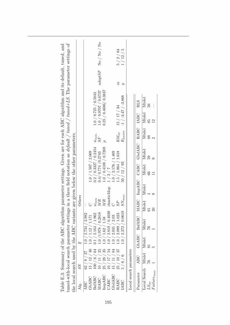
Tab
leE
.3:
Sum
mar
yof
the
AB
Cal
gori
thm
par
amet
erse
ttin
gs.
Giv
enar
efo
rea
chA
BC
algo
rith
man
dit
sdef
ault
,tu
ned
,an
dtu
ned
-wit
h-l
oca
lse
arch
par
amet
erse
ttin
gsin
ath
ree
fiel
dnot
atio
nas
defa
ult
/tu
ned
/tu
ned
+L
S.
The
par
amet
erse
ttin
gsof
the
loca
lse
arch
use
dby
the
AB
Cva
rian
tsar
egi
ven
bel
owth
eot
her
par
amet
ers.
Alg
.SN
lfO
ther
s
AB
C62
/8
/37
1.0
/2.
734
/2.
982
—G
bA
BC
15/
12/
401.
0/
1.12
/1.
171
C1.0
/1.5
07
/2.0
69
Bsf
AB
C10
0/
6/
640.
1/
2.16
4/
1.96
2wmin
0.2
/0.3
327
/0.2
454
wmin
1.0
/0.7
25
/0.5
843
MA
BC
10/
11/
251.
0/1
.978
/0.
2818
MR
0.4
/0.7
74
/0.2
743
SF
1.0
/0.9
707
/0.6
737
adaptSF
No
/N
o/
No
Imp
AB
C25
/28
/35
1.0
/1.
62/
1.58
MR
1.0
/0.4
108
/0.7
269
p0.2
5/
0.4
686/
0.3
837
CA
BC
10/
17/
541.
0/
2.81
9/
0.40
39ch
aoti
cMap
1/
3/
7G
bd
AB
C15
/11
/84
1.0
/2.
031
/2.
03C
1.0
/2.1
76
/1.4
69
RA
BC
25/
10/
371.
0/
2.08
9/
1.02
3SP
1.5
/1.8
64
/1.6
18
RMitr
15
/17
/34
m5
/2
/64
IAB
C5
/6
/6
1.0
/2.
272
/0.
0619
SNmax
50
/12
/93
Rfactor
-1/
-3.4
7/
-3.8
68
g1
/12
/5
Loca
lse
arch
par
amet
ers
Par
amet
erA
BC
Gb
AB
CB
sfA
BC
MA
BC
Imp
AB
CC
AB
CG
bd
AB
CR
AB
CIA
BC
RL
S
Loca
lS
earc
hM
tsls
1M
tsls
1M
tsls
1M
tsls
1M
tsls
1M
tsls
1M
tsls
1M
tsls
1M
tsls
1M
tsls
1LSitr
7681
7661
466
59
88
85
56
Failuremax
15
120
911
92
12
—
195

E. ARTIFICIAL BEE COLONIES FOR CONTINUOUS OPTIMIZATION:EXPERIMENTAL ANALYSIS AND IMPROVEMENTS
local search (right column). To obtain these ranks, the results of all variants on a
same benchmark function were ranked from best (rank 1) to worst (rank 9) and
in Figure E.3 are given the so obtained average ranks for each algorithm.
Considering the box-plots for the default parameter settings in dimension 10
(top left plot in Figure E.1), we can observe that all variants except BsfABC
reach typically lower median errors that the original ABC algorithm, which is
confirmed by the average ranks (top left plot in Figure E.3). (The reasons for
the poor performance of BsfABC are given in the next Section.) The overall best
performing ABC variants in this setting and dimension are GbABC and GbdABC,
which indicates that a strong emphasis on the global-best solution is important on
the SOCO benchmark set.
The situation changes a bit when comparing the results obtained by the tuned
parameter settings for dimension 10 (middle plots on top in Figures E.1 and E.3).
In that case, the potential advantage of the ABC variants over the original ABC
diminishes, with the original ABC reaching a ranking similar to that of MABC,
BsfABC, and CABC. In addition, the gap to GbABC and GbdABC, which remain
among the best performers, is reduced. Nevertheless, several ABC variants still
reach statistically significantly better results than the original ABC algorithm, even
if according to the rank information the performance gap is reduced. Among the
tuned versions, ImpABC is the second best ranking, while for default settings it was
the fifth ranked. The introduction of an effective local search procedure reduces
further the gaps between the ABC variants and none of the variants emerges as
a clear winner. Particularly high performance reaches ImpABC, which obtains
on 15 of the 19 benchmark problems a median error value that is lower than
the optimum threshold. Nevertheless, once local search is added no ABC variant
reaches a statistically significanltly improved performance over the original ABC
hybridized with local search.
Considering the scaling behavior of the ABC variants from the ten dimensional
problems up to the 500 dimensional ones, the most noteworthy result is the poor
scaling behavior of MABC and ImpABC, which are for high dimensional problems
among the worst ranked ABC algorithms. In fact, considering default parameter
settings, ImpABC ranks worse than ABC for dimensions 50, 100, and 500 and
MABC ranks worse than ABC for dimension 500; often, the observed differences
are also statistically significant. BsfABC remains the worst ranking ABC algo-
rithm. Taking into account the differences in the absolute values as indicated by
the boxplots or the numerical results in Tables E.4 to E.7, the differences in solu-
tion quality are substantial. The same poor scaling behavior for ImpABC, MABC
196

ABC
GbABC
BsfABC
MABC
ImpABC
CABC
GbdABC
RABC
IABC
1e−
14
1e−
09
1e−
04
1e+
01
1e+
06
++
++
+−
Optim
a0
11
011
10
512
63
Median Errors of Fitness Value
10dim
ensio
ns−
dp
ABC
GbABC
BsfABC
MABC
ImpABC
CABC
GbdABC
RABC
IABC
1e−
14
1e−
09
1e−
04
1e+
01
1e+
06
++
++
+O
ptim
a8
11
610
15
714
12
11
Median Errors of Fitness Value
10dim
ensio
ns−
ts
ABC
GbABC
BsfABC
MABC
ImpABC
CABC
GbdABC
RABC
IABC
1e−
14
1e−
09
1e−
04
1e+
01
1e+
06
Optim
a12
11
13
12
15
13
11
11
12
Median Errors of Fitness Value
10dim
ensio
ns−
ts: +
LS
ABC
GbABC
BsfABC
MABC
ImpABC
CABC
GbdABC
RABC
IABC
1e−
14
1e−
09
1e−
04
1e+
01
1e+
06
++
++
+−
−O
ptim
a0
14
07
06
14
43
Median Errors of Fitness Value
50dim
ensio
ns−
dp
ABC
GbABC
BsfABC
MABC
ImpABC
CABC
GbdABC
RABC
IABC
1e−
14
1e−
09
1e−
04
1e+
01
1e+
06
+−
−−
Optim
a8
14
45
28
13
914
Median Errors of Fitness Value
50dim
ensio
ns−
ts
ABC
GbABC
BsfABC
MABC
ImpABC
CABC
GbdABC
RABC
IABC
1e−
14
1e−
09
1e−
04
1e+
01
1e+
06
Optim
a14
14
14
12
913
12
14
14
Median Errors of Fitness Value
50dim
ensio
ns−
ts: +
LS
Fig
ure
E.1
:B
oxplo
tsof
the
dis
trib
uti
onof
the
med
ian
solu
tion
qual
ity
reac
hed
by
each
ofth
est
udie
dA
BC
vari
ants
onth
e19
SO
CO
ben
chm
ark
pro
ble
ms.
The
num
ber
onto
pof
each
box
give
sth
enum
ber
offu
nct
ions
onw
hic
hth
em
edia
ner
ror
found
was
bel
owth
eop
tim
um
thre
shol
dof
10−
14.
The
box
plo
ton
the
top
row
are
for
funct
ions
ofdim
ensi
on10
;th
eb
oxplo
tson
the
bot
tom
row
are
for
funct
ions
ofdim
ensi
on50
.A
“+”
or“−
”sy
mb
olon
top
ofa
box
-plo
tden
otes
asi
gnifi
cant
diff
eren
cedet
ecte
dby
aW
ilco
xon
’ste
stat
the
0.05
leve
lw
ith
Hol
m’s
corr
ecti
onfo
rm
ult
iple
test
ing
bet
wee
nth
ere
sult
sob
tain
edw
ith
indic
ated
algo
rith
man
dth
eor
igin
alA
BC
algo
rith
m(fi
rst
box
)).
197

E. ARTIFICIAL BEE COLONIES FOR CONTINUOUS OPTIMIZATION:EXPERIMENTAL ANALYSIS AND IMPROVEMENTS
and BsfABC is observed for the tuned parameter settings. In section E.4.2, we
identify the reason for this poor scaling behavior and indicate the remedy. GbABC
and GbdABC remain among the best performing ABC algorithms also for higher
dimensional problems, showing that the emphasis on the global-best solution is
important for a good scaling behavior. Interestingly, for higher dimensional prob-
lems, IABC algorithm becomes the best ranking one and it is one of the ABC
algorithms that profit most from tuning. Finally, considering the ABC variants
with local search, their performance levels remain comparable and no statistically
significant differences in favor of any of the ABC variants over the original ABC
with local search are detected.
The main results of our comparison of ABC variants can be summarized as
follows.
• Tuning has a major impact on the comparison results. In fact, especially on
the higher dimensional benchmark problems several of the proposed ABC
algorithm variants do not give a statistically significant improvement over
the original ABC algorithm, once one considers reasonably tuned parameter
settings.
• The introduction of a local search smoothes the differences between the dif-
ferent ABC variants and poor performing ones without local search become
very competitive to the best ABC variants.
• Some of the variants such as BsfABC perform surprisingly poor when com-
pared to the original papers. Some of the variants appear to have poor
scaling behavior.
In the following section, we revist some of the above made conclusions and
provide a more detailed analysis of several ABC variants.
E.4.2 Detailed analysis of ABC algorithms
Improvement over random restart local search
The best performing ABC algorithms typically include local search, as shown in the
previous section. Hence, a first question that arises is whether the ABC algorithms
contribute significantly to performance or whether the local search alone is enough
to reach a same performance level. We explore this question by comparing the
hybrid ABC algorithms to a random restart local search (RLS) algorithm, where
198

ABC
GbABC
BsfABC
MABC
ImpABC
CABC
GbdABC
RABC
IABC
1e−
14
1e−
09
1e−
04
1e+
01
1e+
06
++
++
+−
−O
ptim
a0
14
05
07
14
43
Median Errors of Fitness Value
100dim
ensio
ns−
dp
ABC
GbABC
BsfABC
MABC
ImpABC
CABC
GbdABC
RABC
IABC
1e−
14
1e−
09
1e−
04
1e+
01
1e+
06
++
−−
−O
ptim
a7
14
32
08
13
912
Median Errors of Fitness Value
100dim
ensio
ns−
ts
ABC
GbABC
BsfABC
MABC
ImpABC
CABC
GbdABC
RABC
IABC
1e−
14
1e−
09
1e−
04
1e+
01
1e+
06
Optim
a13
14
13
12
612
12
14
14
Median Errors of Fitness Value
100dim
ensio
ns−
ts: +
LS
ABC
GbABC
BsfABC
MABC
ImpABC
CABC
GbdABC
RABC
IABC
1e−
14
1e−
09
1e−
04
1e+
01
1e+
06
++
++
+−
−−
Optim
a0
12
00
07
12
33
Median Errors of Fitness Value
500dim
ensio
ns−
dp
ABC
GbABC
BsfABC
MABC
ImpABC
CABC
GbdABC
RABC
IABC
1e−
14
1e−
09
1e−
04
1e+
01
1e+
06
++
−−
−O
ptim
a7
12
20
07
87
12
Median Errors of Fitness Value
500dim
ensio
ns−
ts
ABC
GbABC
BsfABC
MABC
ImpABC
CABC
GbdABC
RABC
IABC
1e−
14
1e−
09
1e−
04
1e+
01
1e+
06
−O
ptim
a12
12
12
11
712
10
12
12
Median Errors of Fitness Value
500dim
ensio
ns−
ts: +
LS
Fig
ure
E.2
:B
oxplo
tsof
the
dis
trib
uti
onof
the
med
ian
solu
tion
qual
ity
reac
hed
by
each
ofth
est
udie
dA
BC
vari
ants
onth
e19
SO
CO
ben
chm
ark
pro
ble
ms.
The
num
ber
onto
pof
each
box
give
sth
enum
ber
offu
nct
ions
onw
hic
hth
em
edia
ner
ror
found
was
bel
owth
eop
tim
um
thre
shol
dof
10−
14.
The
box
plo
ton
the
top
row
are
for
funct
ions
ofdim
ensi
on10
0;th
eb
oxplo
tson
the
bot
tom
row
are
for
funct
ions
ofdim
ensi
on50
0.A
“+”
or“−
”sy
mb
olon
top
ofa
box
-plo
tden
otes
asi
gnifi
cant
diff
eren
cedet
ecte
dby
aW
ilco
xon
’ste
stat
the
0.05
leve
lw
ith
Hol
m’s
corr
ecti
onfo
rm
ult
iple
test
ing
bet
wee
nth
ere
sult
sob
tain
edw
ith
indic
ated
algo
rith
man
dth
eor
igin
alA
BC
algo
rith
m(fi
rst
box
)).
199

E. ARTIFICIAL BEE COLONIES FOR CONTINUOUS OPTIMIZATION:EXPERIMENTAL ANALYSIS AND IMPROVEMENTS
AB
C
Gb
AB
C
BsfA
BC
MA
BC
Imp
AB
C
CA
BC
Gb
dA
BC
RA
BC
IAB
C
10Dim−Median Errors−dp
Ra
nk
24
68
10
7.1
3.4
8.9
4.1
4.8
5.9
2.4
3.6
4.9
optima 0 11 0 11 10 5 12 6 3
AB
C
Gb
AB
C
BsfA
BC
MA
BC
Imp
AB
C
CA
BC
Gb
dA
BC
RA
BC
IAB
C
10Dim−Median Errors−ts
Ra
nk
24
68
10
6.3
4.1
6.8
5.5
3.8
5.9
3.4
4.84.4
optima 8 11 6 10 15 7 14 12 11
AB
C
Gb
AB
C
BsfA
BC
MA
BC
Imp
AB
C
CA
BC
Gb
dA
BC
RA
BC
IAB
C
10Dim−Median Errors−ts +LS
Ra
nk
24
68
10
4.6
5.7
4.75.3
4.2 4.3
5.95.2 5
optima 12 11 13 12 15 13 11 11 12A
BC
Gb
AB
C
BsfA
BC
MA
BC
Imp
AB
C
CA
BC
Gb
dA
BC
RA
BC
IAB
C50Dim−Median Errors−dp
Ra
nk
24
68
10
7
2.7
8.3
5.1
7.6
3.7
2.4
3.4
4.8
optima 0 14 0 7 0 6 14 4 3
AB
C
Gb
AB
C
BsfA
BC
MA
BC
Imp
AB
C
CA
BC
Gb
dA
BC
RA
BC
IAB
C
50Dim−Median Errors−ts
Ra
nk
24
68
10
4.4
3.5
6.6 7
7.9
4.3
3.6
4.3
3.3
optima 8 14 4 5 2 8 13 9 14
AB
C
Gb
AB
C
BsfA
BC
MA
BC
Imp
AB
C
CA
BC
Gb
dA
BC
RA
BC
IAB
C
50Dim−Median Errors−ts +LS
Ra
nk
24
68
10
4.54.2
4.7
5.56.1
5.3 5.6
4.34.8
optima 14 14 14 12 9 13 12 14 14
AB
C
Gb
AB
C
BsfA
BC
MA
BC
Imp
AB
C
CA
BC
Gb
dA
BC
RA
BC
IAB
C
100Dim−Median Errors−dp
Ra
nk
24
68
10
6.7
2.6
8.3
5.7
7.7
3.6
2.6
3.2
4.6
optima 0 14 0 5 0 7 14 4 3
AB
C
Gb
AB
C
BsfA
BC
MA
BC
Imp
AB
C
CA
BC
Gb
dA
BC
RA
BC
IAB
C
100Dim−Median Errors−ts
Ra
nk
24
68
10
4.5
3.3
6.6
7.78.2
4.1
3.33.9
3.4
optima 7 14 3 2 0 8 13 9 12
AB
C
Gb
AB
C
BsfA
BC
MA
BC
Imp
AB
C
CA
BC
Gb
dA
BC
RA
BC
IAB
C
100Dim−Median Errors−ts +LS
Ra
nk
24
68
10
5.2
3.8
4.75.1
6.6
5.4 5.6
4.4 4.2
optima 13 14 13 12 6 12 12 14 14
AB
C
Gb
AB
C
BsfA
BC
MA
BC
Imp
AB
C
CA
BC
Gb
dA
BC
RA
BC
IAB
C
500Dim−Median Errors−dp
Ra
nk
24
68
10
6.3
2.5
7.87.2
7.7
3.12.7
3.5
4.3
optima 0 12 0 0 0 7 12 3 3
AB
C
Gb
AB
C
BsfA
BC
MA
BC
Imp
AB
C
CA
BC
Gb
dA
BC
RA
BC
IAB
C
500Dim−Median Errors−ts
Ra
nk
24
68
10
4.2
3.2
6.1
8.2 8.1
3.4
4.3 4.5
2.9
optima 7 12 2 0 0 7 8 7 12
AB
C
Gb
AB
C
BsfA
BC
MA
BC
Imp
AB
C
CA
BC
Gb
dA
BC
RA
BC
IAB
C
500Dim−Median Errors−ts +LS
Ra
nk
24
68
10
4.8 4.6 4.5
5.4
6.3
4.8
5.5
4.6 4.4
optima 12 12 12 11 7 12 10 12 12
Figure E.3: Performance comparisons by the means of the average rank over 19functions. The ranking was based on the median error value of obtained by eachalgorithm on the 19 SOCO benchmark functions.
the starting points for the local search are generated uniformly at random in the
search space. To make the comparison fair, we tuned the parameters of the RLS
algorithm, which are the parameters of the Mtsls1 local search algorithm [Tseng
and Chen, 2008], using the same procedure and tuning budget as used when tuning
the ABC algorithms. The tuned parameter settings of RLS are given in Table E.3,
page 195.
Figure E.4 summarizes the results of this comparison across several dimensions
of the benchmark functions. A “−” symbol on top of a box denotes that RLS
performs statistically significantly worse than the respective ABC algorithm. As
200

we see in Figure E.4, RLS gives worse results in all dimensions. In fact, the
local search alone is able on only few functions (f1, f4, f5, and f10 of the SOCO
benchmark set) to find solutions better then the optimum threshold, while for the
ABC algorithms this is the case for often more than ten functions. Except for a few
ABC variants, the observed differences are statistically significant. Therefore, we
may conclude that there is an overall synergetic effect between the ABC algorithms
and the local search.
AB
C
Gb
AB
C
BsfA
BC
MA
BC
Imp
AB
C
CA
BC
Gb
dA
BC
RA
BC
IAB
C
RL
S
1e−14
1e−09
1e−04
1e+01
1e+06
RLS − − − −
Optima 12 11 13 12 15 13 11 11 12 6
10dimensions−ts: +LS
Me
dia
n E
rro
rs o
f F
itn
ess V
alu
e
AB
C
Gb
AB
C
BsfA
BC
MA
BC
Imp
AB
C
CA
BC
Gb
dA
BC
RA
BC
IAB
C
RL
S
1e−14
1e−09
1e−04
1e+01
1e+06
RLS − − − − − − − −
Optima 14 14 14 12 9 13 12 14 14 4
50dimensions−ts: +LS
Me
dia
n E
rro
rs o
f F
itn
ess V
alu
e
AB
C
Gb
AB
C
BsfA
BC
MA
BC
Imp
AB
C
CA
BC
Gb
dA
BC
RA
BC
IAB
C
RL
S
1e−14
1e−09
1e−04
1e+01
1e+06
RLS − − − − − − − −
Optima 13 14 13 12 6 12 12 14 14 4
100dimensions−ts: +LS
Me
dia
n E
rro
rs o
f F
itn
ess V
alu
e
AB
C
Gb
AB
C
BsfA
BC
MA
BC
Imp
AB
C
CA
BC
Gb
dA
BC
RA
BC
IAB
C
RL
S
1e−14
1e−09
1e−04
1e+01
1e+06
RLS − − − − − − − −
Optima 12 12 12 11 7 12 10 12 12 4
500dimensions−ts: +LS
Me
dia
n E
rro
rs o
f F
itn
ess V
alu
e
Figure E.4: Performance comparisons with RLS. A “−” symbol on top of a box-plot denotes a significant difference detected by a Wilcoxon’s test at the 0.05level (using Holm’s correction) between the results obtained with the indicatedalgorithm and RLS.
Original ABC algorithm
As shown in the previous section, the original ABC algorithm can profit quite
strongly from parameter tuning and reach performance that is similar to various of
its extensions that have been proposed as improvements. This result also illustrates
the danger of comparing to a default version of ABC and we recommend that
201

E. ARTIFICIAL BEE COLONIES FOR CONTINUOUS OPTIMIZATION:EXPERIMENTAL ANALYSIS AND IMPROVEMENTS
in future papers on potential improvements over ABC, the original version and
the modified version is automatically tuned to avoid biases by the designer of a
particular extension.
Already in earlier papers, the impact of parameter settings on the performance
of ABC was studied [Akay and Karaboga, 2009, Diwold et al., 2011a, Karaboga
and Basturk, 2008]. Conclusions were, for example, that a too low value of the
limit parameter leads to poor performance, that ABC’s performance is relatively
robust given the limit value as determined through parameter lf is large enough
[Akay and Karaboga, 2009, Diwold et al., 2011a], and that the population size
does not need to be fine-tuned in order to obtain satisfactorily good results [Akay
and Karaboga, 2009]. Our results indicate, however, that even the original ABC
algorithm can profit substantially from a further fine-tuning of its parameters.
Global-best and global-best distance ABC
The GbABC and GbdABC algorithms did not profit much or at all from the
additional parameter tuning. This can be seen in the bottom part of Tables E.4
to E.7 at the summary statistics on the number of functions that obtain better,
same or worse median quality after tuning or the additional introduction of local
search. This indicates that either their design makes them rather robust w.r.t.
modified parameter settings or that the original authors have already very well
fine-tuned the parameter settings. In fact, the tuned parameter settings at least
for GbABC are rather similar to the ones proposed as default settings, giving some
evidence for the latter. Interestingly, for GbABC and GbdABC the additional local
search phase does actually slightly (though not significantly) worsen performance.
This indicates that ABC algorithms that use appropriate algorithm features and
that are well parameterized do not necessarily require an additional local search
phase to reach very high performance on the SOCO benchmark set.
Best-so-far ABC
The poor performance of BsfABC we observed is in apparent contradiction to
the excellent results reported in the original paper by Banharnsakun et al. [2011].
However, these differences can be explained by particularities in the design of
BsfABC. As mentioned in Section E.2.2, BsfABC applies a position update to
each dimension in such a way that the variable values in all dimensions get closer
to each other. This induces a strong bias towards solving well problems where
the optimum has in all dimensions the same variable values. In particular, in
202

Function evaluations
Me
dia
n e
rro
r va
lue
100
101
102
103
104
5 × 1041
e−
14
1e
−0
61
e+
02
shift
noshfit
BsfABC−f1−10D
Function evaluations
Me
dia
n e
rro
r va
lue
100
101
102
103
104
5 × 1041
e−
14
1e
−1
01
e−
06
1e
−0
21
e+
02
shift
noshfit
BsfABC−f4−10D
Figure E.5: Development of the median solution value over time for BsfABC onthe ten dimensional SOCO functions f1 (Sphere, left plot) and f4 (Rastrigin, rightplot) for the shifted and the unshifted versions. The unshifted version has theoptimum at the point (0, . . . , 0).
the experiments reported in Banharnsakun et al. [2011] the benchmark problems
have the optimum in the solution x = (0, . . . , 0), while the benchmark problems in
the SOCO benchmark set have their optimum randomly shifted within the search
range.
In Figure E.5 we show the development of the median error value over the
number of function evaluations for the shifted and the not-shifted version of two
SOCO benchmark functions (Sphere–f1–and Rastrigin–f4, respectively). As ex-
pected, the fact whether the optimum of a function is randomly shifted in the
search range (the shift is independently done for each dimension) or not, has a
huge impact in the performance of BsfABC, which is only effective for problems
where the optimum solutions have a same variable value in each dimension. The
same experiments with the other ABC variants did not show a significant influ-
ence of an optimum shift on performance. Finally, after tuning the performance
of BsfABC is strongly improved; this is probably due to the larger setting of lf
and the smaller population size.
Improved and Modified ABC
For functions of ten dimensions, MABC and, in particular, ImpABC show good
results; in fact, on ten dimensions, the tuned version of ImpABC and ImpABC with
local search are the best ranking ABC algorithms. However, the good performance
of ImpABC and also MABC decline quickly with increasing dimensionality of the
benchmark problems. For example, the tuned version of ImpABC is the worst
203
E. ARTIFICIAL BEE COLONIES FOR CONTINUOUS OPTIMIZATION:EXPERIMENTAL ANALYSIS AND IMPROVEMENTS
ranking ABC algorithm for 50 and 100 dimensional problems and the only ABC
algorithms whose median is not below the optimum threshold of any function for
100 dimensional problems. Similary, the performance of ImpABC and MABC
with local search declines with high dimensional functions, though less due to
the mitigating effect of the local search. In other words, the scaling behavior of
ImpABC and MABC is poor. As the main reason for this poor scaling behavior
we identified the choice of increasing the number of variables that are modified
with the dimension of the functions. In fact, if only a small, constant number
of variables is modified, the scaling behavior of MABC and ImpABC improves
strongly to an extent to which ImpABC and MABC become competitive with the
other ABC algorithms (see also the supplementary pages http://iridia.ulb.
ac.be/supp/IridiaSupp2013-002).
The improvements incurred by keeping the number of variables modified to a
constant value is shown for MABC in Figure E.6 and for ImpABC in Figure E.7.
In each of these plots we compare the median error values of MABC and ImpABC
using default parameter settings except that the number of variables to be changed
is set to eight for MABC and four for ImpABC, as suggested by the tuning on
the ten dimensional problems. We refer to the latter variants as MABC-new and
ImpABC-new.
Another explanation for the poor scaling behavior resides in the fact that the
training set comprised only functions of a fixed dimensionality. Hence, the tuning
cannot detect whether it is better to set the parameter to a constant or to scale
it with the dimensionality of the problems. Thus, more advanced possibilities for
scaling parameters would have to be considered.
Chaotic ABC
After tuning, the performance of CABC is improved compared to the default
parameter settings. However, the original ABC benefits even more from tuning so
that once tuned, CABC does not show anymore a significant improvement over the
original ABC version, drawing some doubt about the real impact of the proposed
modifications.
Rosenbrock ABC
RABC is the only ABC algorithm we included in the comparison that in its origi-
nal form makes use of a local search procedure. While on dimension 10 it obtains
on several functions better median performance than the tuned original ABC algo-
204

rithm (better on nine and worse on two), for larger dimensions it is roughly on par
with the original ABC, despite making use of the Rosenbrock rotational direction
method (RM). One reason may be that RM is not a very effective local search
method for the benchmark problems tested here. In fact, after adding the Mtsls1
local search, the resulting hybrid RABC improves strongly its performance, giving
some indication that this conjecture is true.
We can also test the effect RM has in RABC by removing it. Interestingly, once
RM is removed from RABC, the only difference from the resulting ABC algorithm
to the original ABC algorithm is the usage of the rank-based probabilistic selection
of a solution by the onlooker bees instead of the usual fitness-based one through
Equation E.4. The impact of this choice on ABC performance can be observed
from the plots in Figure E.8, where the parameter settings correspond to the tuned
settings of the original ABC algorithm. In fact, replacing the fitness-based selection
by the rank-based probabilistic selection of solutions leads for all dimensions to
improved performance (being statistically significant in dimensions 10 and 100).
Incremental ABC
IABC performs generally better than the original ABC algorithm, reaching on 11
of the 19 functions of dimension 10 better median results. Similarly, on the higher
dimensional functions it improves on either 10 or 11 functions over the original
ABC and is only worse on one function (f2). The strong improvement through
the tuning is probably due to the lower limit on the maximum population size in
IABC and the slower increase of the population size when compared to the default
parameter settings. Overall, it belongs to the best ranking ABC variants.
Solution behavior of the ABC variants
Next, we examine the development of the solution quality over time by so called
SQT plots [Hoos and Stutzle, 2005]. In particular, we give the development of
the median error over computation time measured by the number of function
evaluation as usual in continuous optimization. First we examine the impact of
parameter tuning and the usage of an additional local search on the behavior
of the ABC algorithms. In Figure E.9 are given representative SQT plots for
the original ABC algorithm, GbABC, and IABC on three functions of dimension
50 (functions f1, f3, and f13 from the SOCO benchmark set, that is, Sphere,
Rosenbrock, and a hybrid function). In these plots we can observe that the tuning
improves strongly the convergence behavior of the original ABC algorithm and
205

E. ARTIFICIAL BEE COLONIES FOR CONTINUOUS OPTIMIZATION:EXPERIMENTAL ANALYSIS AND IMPROVEMENTS
IABC, while GbABC is almost not affected by the tuning, which can be noticed by
the, in part, overlapping curves for the default and the tuned version. Additional
local search may further speed up convergence towards high quality solutions as
noticed by the fact that these curves are typically left-most in the plots. However,
the additional local search does not always improve the final solution quality as
can be noticed, for example, on the plots for function f13.
In addition to SQT plots, we have generated run-time distributions (RTDs)
for reaching the optimum threshold (or other very high quality solutions) and
solution-quality distributions (SQDs) [Hoos and Stutzle, 2005]. In Figure E.10 we
give few RTDs for the same three algorithms with tuned parameter settings and
hybridized with local search on benchmark functions f5 and f6. The RTDs on
benchmark function f5 indicate that the ABC variants suffer in part from severe
stagnation behavior. The most extreme is IABC with local search: after less than
2000 function evaluations it finds in almost 50% of the runs a solution better
than the optimum threshold but in the remaining, much longer runs it hardly
finds additional optima. The RTDs on benchmark function f5 are also interesting
because they show how the ranking of the variants changes depending on whether
local search is used or not: on f5 actually the original ABC with local search
performs better than the other two algorithms with local search, while without
local search IABC and GbABC are clearly better than original ABC. The RTDs
on f6 are more representative for RTDs on the majority of the functions: with local
search the various variants have rather similar performance, while without local
search differences are still more apparent. Typcial is also that for many functions
the ABC variants do not really show stagnation behavior (see also supplementary
pages http://iridia.ulb.ac.be/supp/IridiaSupp2013-002).
Finally, Figure E.11 gives two SQDs for benchmark function f5, which cor-
respond to the distribution of the solution quality at the maximum number of
function evaluations. These SQDs confirm the stagnation behavior showing that
some runs are trapped in strongly sub-optimal solutions, an effect that is most
visible in the SQDs for ABC variants with local search. In fact, we conjecture that
by either changing the scheme of local search application to more frequently choose
other than the global-best solution or some partial algorithm restart feature could
be useful to enhance algorithm performance in such cases.
206

E.4.3 Comparison with SOCO special issue contributors
As a final step, we compare one of the best performing ABC variants with lo-
cal search to all algorithms that have been contributed to the Soft Computing
special issue Lozano et al. [2011]. All along our experiments in this chapter, we
used actually the same experimental setup as proposed for this special issue and,
hence, such a comparison is fair in this respect. The results of 13 algorithms have
been published in the special issue. In addition, three benchmark algorithms had
been included as reference algorithms to which each entry to the special issue
had to be compared and which each competitor should have outperformed. These
three reference algorithms were a differential evolution algorithm [Stern and Price,
1997], the real-coded CHC algorithm [Eshelman and Schaffer, 1993], and G-CMA-
ES [Auger and Hansen, 2005]. In particular, G-CMA-ES was the best performing
algorithm in the special session on real parameter optimization of the 2005 IEEE
Congress on Evolutionary Computation (CEC’05) and the MA-SSW algorithm
Molina et al. [2011], one of the 13 algorithms published in the SOCO special issue,
was the best performing algorithm at the CEC 2010 special session on large scale
global optimization. Hence, the algorithms to which we compare can be considered
representatives of the state-of-the-art in real parameter optimization.
For this comparison we have chosen GbABC with local search as it is one of
the best ABC algorithms across various dimensions and it is still a rather straight-
forward variant. We have computed for all the algorithms the distribution of the
median error values found from the publicly available results tables and the box-
plots in Figure E.12 compare these distributions across several dimensions. In fact,
GbABC reaches a median performance that is competitive to the best continuous
optimizers from the competition; for example, it reaches for 50 and 100 dimensions
a median error that is below the optimum threshold for 14 functions, the same
as the overall best performing algorithm in the benchmark competition, MOS-DE
[LaTorre et al., 2011]. A further statistical analysis (using Wilcoxon’s test with
Holm’s correction for multiple comparisons) shows that GbABC is statistically
significantly better than reference algorithms DE, CHC and G-CMA-ES as well
as some contributors such as SOUPDE, GODE, MA-SSW, RPSO-vm, EvoPROpt
and EM323 for dimensions 100 and 500. Hence, when considering median perfor-
mance, GbABC (and actually also several other ABC algorithms, such as IABC,
which have very similar performance to GbABC) are competitive with state-of-
the-art algorithms for large-scale continuous optimization problems.
The good median performance is in part due to the fact that the tuning is
207

E. ARTIFICIAL BEE COLONIES FOR CONTINUOUS OPTIMIZATION:EXPERIMENTAL ANALYSIS AND IMPROVEMENTS
done using F-race, a rank-based method. If the algorithms are compared based
on mean error values, GbABC is still among the best performing ones but com-
pares worse, for example, to MOS-DE than when using median error values.
(A comparison of GbABC to the other algorithms from the SOCO special is-
sue based on mean error values is available on the chapter’s supplementary pages
http://iridia.ulb.ac.be/supp/IridiaSupp2013-002.) The main reason for
the worse mean performance is due to the stagnation of the algorithm in some
runs on few functions. It would be interesting to re-tune the algorithms based on,
for example, t-race which implicitly will favor algorithms having better average
behavior.
E.5 Discussion and conclusions
In this chapter, we have reviewed artificial bee colony (ABC) optimization algo-
rithms for continuous optimization and we have examined various of the proposed
ABC experimentally using a recent benchmark function set for large-scale con-
tinuous optimization. Our experimental analysis is based on re-implementations
of nine ABC algorithms including the original one, which are compared under
same computational conditions. The ABC variants were compared using three
setups. First, using their default parameter settings; second, using an automatic
algorithm configuration tool to determine parameter settings; third, by combining
the ABC algorithms with local search and re-tuning their parameter settings by
an automatic algorithm configuration tool. The usage of an automatic algorithm
configuration tool in our context has essentially three main reasons. The first is
to potentially improve significantly the default algorithm parameter settings; this
was actually achieved for most of the ABC variants. The second reason is to avoid
the bias in results due to an uneven tuning of the different algorithm variants;
this was achieved by using a same tuning setup and effort for all algorithms. A
third reason is to help in the design of hybrid ABC algorithms that include an
effective local search for continuous optimization; this was necessary due to the
fact that nine hybrid algorithms had to be designed. The high performance of the
final hybrid algorithms justifies a posteriori this procedure.
Some of the main results of our experimental analysis and comparison are the
following. First, when considering default parameter settings and low dimensional
benchmark problems, most of the ABC variants actually improve over the original
ABC algorithm, as would be promised by the original papers where the variants
208
have been proposed.1
However, this conclusion changes as we move from to tuned parameter settings
and to the ABC variants with local search or as we move to higher-dimensional
problems. Considering tuned parameter settings, several of the proposed ABC
variants do not result anymore in significantly improved performance (especially
in higher dimensional problems). The situation gets even “worse” if we move to
the ABC variants that include an effective local search algorithm. In fact, no
statistically significant differences of the hybrid ABC variants to the original ABC
with local search are detected anymore when measuring performance by the median
error value. This result is due to the fact that an effective local search typically
smoothes the performance differences between algorithms without local search. In
fact, we could claim that as a side-product of our experimental analysis, we have
derived a number of new state-of-the-art ABC algorithms, as most of the high-
performing, hybrid ABC algorithms we examine have never been considered before.
However, the particular scheme we used of adding local search to ABC algorithms
has been examined before in other contexts [Aydın et al., 2012, Liao et al., 2011b,
Montes de Oca et al., 2011] and the resulting high performance actually is rather
an indication that this particular hybridization scheme is promising. A maybe
surprising result is that few of the ABC variants that we examined do not profit
really from the additional local search phase but reach very high performance
without. This is the case for GbABC and GbdABC and it suggests that ABC
algorithms, if appropriately configured and tuned have already a very strong local
search behavior.
If we move from the low-dimensional problems to higher-dimensional ones, we
observed that some of the proposed ABC variants have rather poor scaling behavior
and become the worst performing ABC algorithms for the highest dimensional
problems we considered. This poor scaling behavior affected mainly modified ABC
[Akay and Karaboga, 2012] and improved ABC [Gao and Liu, 2011]. However, we
could identify that the underlying reason was a particular choice in the setting
of a specific parameter that scaled with the dimensionality (see Section E.4.2);
by keeping the parameter simply to a constant, the scaling behavior of these two
variants was largely improved making them competitive to the other variants for
high dimensional functions.
In a final step, we compared the median error values obtained by one of the
1An exception is the best-so-far ABC algorithm [Banharnsakun et al., 2011] for which wehave observed poor performance. In Section E.4.2 we have shown that this poor behavior is dueto specific choices in the algorithm design.
209

E. ARTIFICIAL BEE COLONIES FOR CONTINUOUS OPTIMIZATION:EXPERIMENTAL ANALYSIS AND IMPROVEMENTS
best performing ABC algorithms, the hybrid GbABC, to the results of a recent
benchmarking effort for high dimensional real function optimization. A result of
this comparison is that the best performing ABC variants we examined are well
competitive with state-of-the-art algorithms for continuous function optimization.
Finally, there is a large number of further work that could be done in the
direction followed here. A straightforward one is to extend the analysis of the
ABC algorithms on other benchmark sets, as, depending on the properties of the
benchmark functions, the relative performance of algorithms may change. In fact,
it would be also interesting to extend the study to other benchmark sets such as
those from the CEC 2005 special session or the Black-Box Optimization Bench-
marking (BBOB) suite. Another direction would be to re-consider the integration
of local search algorithms into ABC algorithms and try to elaborate a more refined
and potentially more performing scheme for integration. The fact that our hybrid
algorithms have shown on some functions stagnation behavior is an indication that
by a more refined design further improvements are possible. Given the existance
of a number of other ABC variants we did not include in our experimental com-
parison, yet another direction would be to extend our experimental study to these.
Nevertheless, we think that more interesting would be the elaboration of a flexible
algorithm framework for ABC algorithms, where the various proposed modifica-
tions to ABC are implemented as algorithm components that may be combined.
Automatic algorithm configuration could then be applied to such a framework to
possibly obtain even more performing algorithms. Such an approach has been ex-
plored for other problems [KhudaBukhsh et al., 2009, Lopez-Ibanez and Stutzle,
2012] and the high performance of our initial effort on configuring hybrid ABC
algorithms with local search just confirm that such an approach is very promising.
210
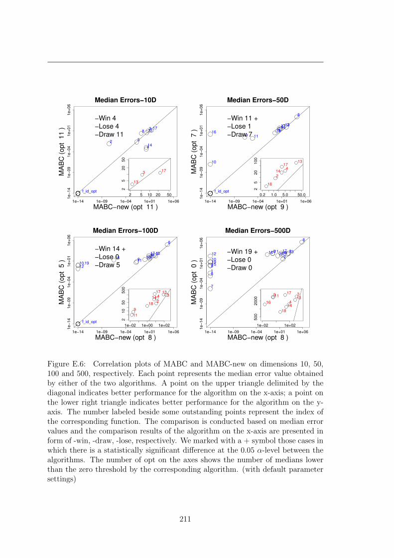
1e−14 1e−09 1e−04 1e+01 1e+06
1e−
14
1e−
09
1e−
04
1e+
01
1e+
06
MABC−new (opt 11 )
MA
BC
(o
pt
11
)
f_id_opt
2
3
4
5
8 13
14
17
−Win 4
−Lose 4
−Draw 11
Median Errors−10D
2 5 10 20 50
25
20
50
3
13
17
1e−14 1e−09 1e−04 1e+01 1e+061e−
14
1e−
09
1e−
04
1e+
01
1e+
06
MABC−new (opt 9 )
MA
BC
(o
pt
7 )
f_id_opt
234
8
9
10
11
1314
16
17
18
−Win 11 +
−Lose 1
−Draw 7
Median Errors−50D
0.2 1.0 5.0 50.0
25
20
100
2
4
18
13
14
17
1e−14 1e−09 1e−04 1e+01 1e+06
1e−
14
1e−
09
1e−
04
1e+
01
1e+
06
MABC−new (opt 8 )
MA
BC
(o
pt
5 )
f_id_opt
234
8
910
11
12
131416
1718
,19
−Win 14 +
−Lose 0
−Draw 5
Median Errors−100D
1e−02 1e+00 1e+02
210
50
500
2
3
9
11
4
18
13
14
17
1e−14 1e−09 1e−04 1e+01 1e+06
1e−
14
1e−
09
1e−
04
1e+
01
1e+
06
MABC−new (opt 8 )
MA
BC
(o
pt
0 )
1
2
34
5
6
7
8
9
10
1112
1314
15
16 1718
19
−Win 19 +
−Lose 0
−Draw 0
Median Errors−500D
1e−02 1e+02
500
2000
3911
16 4
18
13
14
17
Figure E.6: Correlation plots of MABC and MABC-new on dimensions 10, 50,100 and 500, respectively. Each point represents the median error value obtainedby either of the two algorithms. A point on the upper triangle delimited by thediagonal indicates better performance for the algorithm on the x-axis; a point onthe lower right triangle indicates better performance for the algorithm on the y-axis. The number labeled beside some outstanding points represent the index ofthe corresponding function. The comparison is conducted based on median errorvalues and the comparison results of the algorithm on the x-axis are presented inform of -win, -draw, -lose, respectively. We marked with a + symbol those cases inwhich there is a statistically significant difference at the 0.05 α-level between thealgorithms. The number of opt on the axes shows the number of medians lowerthan the zero threshold by the corresponding algorithm. (with default parametersettings)
211

E. ARTIFICIAL BEE COLONIES FOR CONTINUOUS OPTIMIZATION:EXPERIMENTAL ANALYSIS AND IMPROVEMENTS
1e−14 1e−09 1e−04 1e+01 1e+06
1e−
14
1e−
09
1e−
04
1e+
01
1e+
06
ImpABC−new (opt 15 )
Imp
AB
C (
op
t 1
0 )
f_id_opt
34
5911
1314
1718
−Win 8 +
−Lose 1
−Draw 10
Median Errors−10D
1e−14 1e−13
0.2
0.5
2.0
5.0
20.0
18
14
411
9
1e−14 1e−09 1e−04 1e+01 1e+06
1e−
14
1e−
09
1e−
04
1e+
01
1e+
06
ImpABC−new (opt 10 )
Imp
AB
C (
op
t 0
)
1
2 3
4
5
6
7
89
10
1112 1314
15
16 1718
19
−Win 17 +
−Lose 2
−Draw 0
Median Errors−50D
1e−14 1e−13
0.2
1.0
5.0
50.0
500.0
91612
61019
15
51
1e−14 1e−09 1e−04 1e+01 1e+06
1e−
14
1e−
09
1e−
04
1e+
01
1e+
06
ImpABC−new (opt 9 )
Imp
AB
C (
op
t 0
) 12
3
4
5
6
7
89
10
1112 1314
15
16 171819
−Win 18 +
−Lose 1
−Draw 0
Median Errors−100D
1e−14 1e−13
5e−
01
5e+
00
5e+
01
5e+
02
1612
61019
15
5
1
1e−14 1e−09 1e−04 1e+01 1e+06
1e−
14
1e−
09
1e−
04
1e+
01
1e+
06
ImpABC−new (opt 7 )
Imp
AB
C (
op
t 0
)
1
2
4
567
8
9
10
1112 14
15
16
17
1819
−Win 19 +
−Lose 0
−Draw 0
Median Errors−500D
1e−14
20
50
200
6
101915
5
7
1e−02 1e+02
1000
2000
4000
2
9 11
164
18
14
Figure E.7: Correlation plots of ImpABC and ImpABC-new on dimensions 10, 50,100 and 500 respectively. For an explanation of the plots see caption of Figure E.6.
212

1e−14 1e−09 1e−04 1e+01 1e+06
1e−
14
1e−
09
1e−
04
1e+
01
1e+
06
ABC−rank (opt 9 )
AB
C (
op
t 8
)
f_id_opt
2
3
5
8
11
12
13
1416
17
18
−Win 11 +
−Lose 0
−Draw 8
Median Errors−10D
0.2 1.0 5.0 50.0
0.2
2.0
20.0 3
13
178
1e−14 1e−09 1e−04 1e+01 1e+06
1e−
14
1e−
09
1e−
04
1e+
01
1e+
06
ABC−rank (opt 13 )
AB
C (
op
t 8
)
f_id_opt
2 34
5
8
12
1314
16
17
18
−Win 7
−Lose 3
−Draw 9
Median Errors−50D
0.2 1.0 5.0 50.0
0.0
20.5
020.0
0
2 3
13
14
17
1e−14 1e−09 1e−04 1e+01 1e+06
1e−
14
1e−
09
1e−
04
1e+
01
1e+
06
ABC−rank (opt 10 )
AB
C (
op
t 7
)
f_id_opt
23
4
8
911
12
1314
16
17
18
−Win 9 +
−Lose 2
−Draw 8
Median Errors−100D
0.5 2.0 10.0 50.0
0.5
5.0
50.0 2 3
181314
17
1e−14 1e−09 1e−04 1e+01 1e+06
1e−
14
1e−
09
1e−
04
1e+
01
1e+
06
ABC−rank (opt 7 )
AB
C (
op
t 7
)
f_id_opt
234
8
9
11
12
1314
16
1718
−Win 7
−Lose 4
−Draw 8
Median Errors−500D
0.5 5.0 50.0 500.0
0.5
5.0
100.0 2
34
18
1314
17
Figure E.8: Correlation plots of ABC and ABC with a rank-based selectionof solutions by onlooker bees (ABC-rank) on dimensions 10, 50, 100 and 500,respectively. The parameter settings used are the tuned settings for ABC. For anexplanation of the plots see caption of Figure E.6.
213

E. ARTIFICIAL BEE COLONIES FOR CONTINUOUS OPTIMIZATION:EXPERIMENTAL ANALYSIS AND IMPROVEMENTS
Function evaluations
Media
n fitness E
rror
Valu
e
100
101
102
103
104
1051
e−
14
1e
−0
91
e−
04
1e
+0
11
e+
06
ABC−dp
ABC−ts
ABC−LS−ts
f1−50D
Function evaluations
Media
n fitness E
rror
Valu
e
100
101
102
103
104
1051
e−
14
1e
−0
91
e−
04
1e
+0
11
e+
06
GbABC−dp
GbABC−ts
GbABC−LS−ts
f1−50D
Function evaluations
Media
n fitness E
rror
Valu
e
100
101
102
103
104
1051
e−
14
1e
−0
91
e−
04
1e
+0
11
e+
06
IABC−dp
IABC−ts
IABC−LS−ts
f1−50D
Function evaluations
Media
n fitness E
rror
Valu
e
100
101
102
103
104
105
1e
+0
11
e+
04
1e
+0
71
e+
10
ABC−dp
ABC−ts
ABC−LS−ts
f3−50D
Function evaluations
Media
n fitness E
rror
Valu
e
100
101
102
103
104
105
1e
+0
01
e+
03
1e
+0
61
e+
09
1e
+1
2
GbABC−dp
GbABC−ts
GbABC−LS−ts
f3−50D
Function evaluations
Media
n fitness E
rror
Valu
e
100
101
102
103
104
1051
e+
00
1e
+0
31
e+
06
1e
+0
91
e+
12
IABC−dp
IABC−ts
IABC−LS−ts
f3−50D
Function evaluations
Media
n fitness E
rror
Valu
e
100
101
102
103
104
105
1e
−0
11
e+
02
1e
+0
51
e+
08
1e
+1
1
ABC−dp
ABC−ts
ABC−LS−ts
f13−50D
Function evaluations
Media
n fitness E
rror
Valu
e
100
101
102
103
104
105
1e
+0
01
e+
03
1e
+0
61
e+
09
GbABC−dp
GbABC−ts
GbABC−LS−ts
f13−50D
Function evaluations
Media
n fitness E
rror
Valu
e
100
101
102
103
104
1051
e−
01
1e
+0
21
e+
05
1e
+0
81
e+
11
IABC−dp
IABC−ts
IABC−LS−ts
f13−50D
Figure E.9: SQD curves for the original ABC (left column), GbABC (middlecolumn), and IABC (right column) for functions f1 (Sphere, top), f3 (Rosenbrock,middle) and f13 (a hybrid function, bottom).
214

f5−50D
Number of function evaluations
Pro
ba
bili
ty o
f so
lvin
g t
he
pro
ble
m
104
1050
.00
.20
.40
.60
.81
.0
ABC
GbABC
IABC
f6−50D
Number of function evaluations
Pro
ba
bili
ty o
f so
lvin
g t
he
pro
ble
m
104
1050
.00
.20
.40
.60
.81
.0
ABC
GbABC
IABC
tuned parameters
f5−50D
Number of function evaluations
Pro
ba
bili
ty o
f so
lvin
g t
he
pro
ble
m
104
1050
.00
.20
.40
.60
.81
.0
ABC
GbABC
IABC
f6−50D
Number of function evaluations
Pro
ba
bili
ty o
f so
lvin
g t
he
pro
ble
m
104
1050
.00
.20
.40
.60
.81
.0
ABC
GbABC
IABC
tuned with local search
Figure E.10: RLDs for the original ABC, GbABC and IABC for functions f5 (leftcolumn) and f6 (right column) using tuned parameter settings (upper row) and incombination with local search (bottom row).
f5−50D
Optimum bound
Pro
ba
bili
ty o
f so
lvin
g t
he
pro
ble
m
1−14
1−10
1−5
10 1000
0.0
0.2
0.4
0.6
0.8
1.0
ABC
GbABC
IABC
f5−50D
Optimum bound
Pro
ba
bili
ty o
f so
lvin
g t
he
pro
ble
m
1−14
1−10
1−5
10 1000
0.0
0.2
0.4
0.6
0.8
1.0
ABC
GbABC
IABC
tuned parameters tuned with local search
Figure E.11: SQDs for the original ABC, GbABC and IABC for function f5 usingtuned parameter settings (left) and in combination with local search (right).
215

E. ARTIFICIAL BEE COLONIES FOR CONTINUOUS OPTIMIZATION:EXPERIMENTAL ANALYSIS AND IMPROVEMENTS
50 dimension
DE
CH
C
G−
CM
A−
ES
SO
UP
DE
DE
−D
40
−M
m
GO
DE
Ga
DE
jDE
lsco
p
Sa
DE
−M
MT
S
MO
S−
DE
MA
−S
SW
RP
SO
−vm
IPS
O−
Pow
ell
Evo
PR
Op
t
EM
32
3
VX
QR
1
Gb
AB
C−
LS
1e−14
1e−09
1e−04
1e+01
1e+06
+ + + + + + +
Optima 6 0 4 9 12 7 10 12 12 14 11 5 9 4 5 6 14
Media
n E
rrors
of F
itness V
alu
e
100 dimension
DE
CH
C
G−
CM
A−
ES
SO
UP
DE
DE
−D
40
−M
m
GO
DE
Ga
DE
jDE
lsco
p
Sa
DE
−M
MT
S
MO
S−
DE
MA
−S
SW
RP
SO
−vm
IPS
O−
Pow
ell
Evo
PR
Op
t
EM
32
3
VX
QR
1
Gb
AB
C−
LS
1e−14
1e−09
1e−04
1e+01
1e+06
+ + + + + + + + + +
Optima 6 0 3 9 11 6 11 12 12 14 10 5 8 3 6 6 14
Media
n E
rrors
of F
itness V
alu
e
500 dimension
DE
CH
C
G−
CM
A−
ES
SO
UP
DE
DE
−D
40
−M
m
GO
DE
Ga
DE
jDE
lsco
p
Sa
DE
−M
MT
S
MO
S−
DE
MA
−S
SW
RP
SO
−vm
IPS
O−
Pow
ell
Evo
PR
Op
t
EM
32
3
VX
QR
1
Gb
AB
C−
LS
1e−14
1e−09
1e−04
1e+01
1e+06
+ + + + + + − + + + + +
Optima 6 0 2 5 8 6 9 12 10 14 4 4 8 2 4 5 12
Media
n E
rrors
of F
itness V
alu
e
Figure E.12: Comparison of tuned GbABC with local search to the algorithmsfrom the SOCO benchmark competition. A “+” symbol on top of a box-plotdenotes a significant difference detected by a Wilcoxon’s test at the 0.05 levelbetween the results obtained GbABC and the indicated 16 reference algorithm. Ifan algorithm is significantly better than the indicated algorithm, a “−” symbol isput on top of a box-plot for indicating this difference.
216

Table E.4: Given are the medians of the various ABC variants on the 10 dimen-sional functions from the SOCO benchmark set for the default parameter settings(upper part), the tuned parameter settings (middle part) and the tuned hybridABC algorithms with local search (bottom part). At the bottom is indicated thenumber of times the tuned parameter settings give lower, same or worse median(win, draw, loss) than default parameter settings (ts vs dp) and the same infor-mation for the comparisons between the hybrids with local search versus defaultparameter settings (LS vs dp) and hybrids with local search versus tuned settings(LS vs ts).
default parameter settings
Function ABC GbABC BsfABC MABC ImpABC CABC GbdABC RABC IABC
f1 8.31E−07 1.00E−14 2.33E+00 1.00E−14 1.00E−14 1.00E−14 1.00E−14 1.00E−14 1.00E−14f2 1.58E+00 1.02E−08 1.93E+01 7.75E−03 1.00E−14 7.18E+00 1.59E−09 9.50E−04 6.67E−01f3 7.16E+00 2.80E+00 1.23E+04 9.69E+00 1.77E+00 1.37E+01 2.07E+00 2.39E+00 2.71E+00f4 7.06E−03 1.00E−14 7.88E+00 3.92E−04 1.99E+00 1.27E−09 1.00E−14 1.00E−14 2.03E−14f5 3.29E−03 2.67E−08 8.38E−01 1.97E−02 5.41E−02 8.62E−03 6.71E−12 7.40E−03 2.34E−04f6 7.53E−03 1.00E−14 3.72E+00 1.00E−14 1.00E−14 1.00E−14 1.00E−14 1.23E−13 7.85E−12f7 5.14E−05 1.00E−14 1.65E−01 1.00E−14 1.00E−14 1.00E−14 1.00E−14 1.00E−14 1.12E−13f8 4.55E+01 6.08E+00 2.99E+02 2.34E+00 1.00E−14 7.86E+01 6.00E−01 1.04E−02 2.61E+01f9 2.37E+00 1.00E−14 1.64E+01 1.00E−14 2.11E−01 5.44E−01 1.00E−14 2.92E−03 2.77E−02f10 1.51E−07 1.00E−14 1.14E+00 1.00E−14 1.00E−14 1.00E−14 1.00E−14 1.00E−14 1.00E−14f11 1.97E+00 1.00E−14 1.50E+01 1.00E−14 1.56E+00 7.20E−01 1.00E−14 3.66E−03 3.37E−02f12 2.57E−01 1.76E−03 6.14E+00 1.00E−14 1.00E−14 3.87E−02 1.00E−14 2.25E−04 1.07E−02f13 3.35E+00 4.32E−01 3.10E+03 3.42E+00 1.36E+01 4.62E+00 1.59E−01 1.29E−01 4.07E−01f14 1.69E−01 1.75E−03 7.12E+00 1.10E−03 3.46E+00 3.03E−02 3.90E−14 2.05E−04 6.45E−03f15 3.15E−05 1.00E−14 1.90E−01 1.00E−14 1.00E−14 1.00E−14 1.00E−14 1.00E−14 6.60E−14f16 7.75E−01 1.00E−14 7.67E+00 1.00E−14 1.00E−14 3.05E−02 1.00E−14 4.53E−04 5.95E−03f17 1.80E+00 6.00E−01 3.39E+01 1.18E+01 4.26E+01 8.42E+00 2.44E−01 5.66E−01 4.83E−01f18 4.30E−01 1.00E−14 3.62E+00 1.00E−14 5.68E+00 1.06E−02 1.00E−14 1.36E−04 2.11E−03f19 2.03E−06 1.00E−14 4.94E−01 1.00E−14 1.00E−14 2.18E−14 1.00E−14 1.00E−14 1.00E−14
tuned parameter settings
Function ABC-ts GbABC-ts BsfABC-ts MABC-ts ImpABC-ts CABC-ts GbdABC-ts RABC-ts IABC-ts
f1 1.00E−14 1.00E−14 1.00E−14 1.00E−14 1.00E−14 1.00E−14 1.00E−14 1.00E−14 1.00E−14f2 1.74E−01 4.21E−12 1.36E−01 9.50E−07 1.00E−14 2.52E−02 2.28E−13 4.26E−14 4.48E−05f3 2.11E+01 2.54E+00 4.09E+01 5.00E+00 5.06E+00 4.68E+00 1.41E+00 1.82E+01 1.11E+01f4 1.00E−14 1.00E−14 9.95E−01 2.00E+00 1.00E−14 1.00E−14 1.00E−14 1.00E−14 1.00E−14f5 1.01E−02 6.86E−09 1.48E−02 3.94E−02 7.40E−03 9.86E−03 1.00E−14 2.22E−02 9.86E−03f6 1.00E−14 1.00E−14 1.00E−14 1.00E−14 1.00E−14 1.00E−14 1.00E−14 1.00E−14 1.00E−14f7 1.00E−14 1.00E−14 1.00E−14 1.00E−14 1.00E−14 1.00E−14 1.00E−14 1.00E−14 1.00E−14f8 7.27E+00 4.62E+00 6.63E+00 9.62E−08 1.00E−14 1.48E+01 1.71E+00 1.00E−14 4.60E+00f9 1.00E−14 1.00E−14 5.59E−06 1.00E−14 1.00E−14 4.74E−05 1.00E−14 1.00E−14 1.00E−14f10 1.00E−14 1.00E−14 1.00E−14 1.00E−14 1.00E−14 1.00E−14 1.00E−14 1.00E−14 1.00E−14f11 5.99E−08 1.00E−14 2.51E−04 1.00E−14 1.00E−14 2.20E−04 1.00E−14 1.00E−14 1.00E−14f12 3.05E−02 1.32E−03 3.09E−02 1.00E−14 1.00E−14 1.15E−02 1.00E−14 1.07E−02 1.08E−07f13 1.20E+00 3.31E−01 6.13E−01 3.44E+00 5.03E+00 7.43E−01 2.59E−01 3.99E+00 2.20E−01f14 1.16E−02 1.61E−03 1.03E+00 1.99E+00 1.00E−14 9.62E−03 1.00E−14 5.30E−05 6.00E−08f15 1.00E−14 1.00E−14 1.00E−14 1.00E−14 1.00E−14 1.00E−14 1.00E−14 1.00E−14 1.00E−14f16 2.92E−03 1.00E−14 1.19E−02 1.00E−14 1.00E−14 7.82E−04 1.00E−14 1.00E−14 1.00E−14f17 1.52E+01 2.73E−01 8.09E−01 2.57E+01 1.91E−11 7.71E−01 2.90E−01 6.86E+00 4.33E+00f18 3.01E−09 1.00E−14 3.23E−05 1.49E−12 1.00E−14 5.36E−06 1.00E−14 1.00E−14 1.00E−14f19 1.00E−14 1.00E−14 1.00E−14 1.00E−14 1.00E−14 1.00E−14 1.00E−14 1.00E−14 1.00E−14
hybrids with local search
Function ABC-LS GbABC-LS BsfABC-LS MABC-LS ImpABC-LS CABC-LS GbdABC-LS RABC-LS IABC-LS
f1 1.00E−14 1.00E−14 1.00E−14 1.00E−14 1.00E−14 1.00E−14 1.00E−14 1.00E−14 1.00E−14f2 1.42E−14 1.42E−14 1.42E−14 1.42E−14 1.00E−14 1.42E−14 1.42E−14 1.42E−14 1.24E−14f3 5.00E+00 3.04E+01 3.47E+01 3.82E+01 2.90E+00 1.15E+01 5.16E+01 4.23E+01 7.17E+01f4 1.00E−14 1.00E−14 1.00E−14 1.00E−14 1.00E−14 1.00E−14 1.00E−14 1.00E−14 1.00E−14f5 1.00E−14 7.40E−03 1.00E−14 1.00E−14 2.71E−02 1.00E−14 1.23E−02 7.40E−03 2.21E−02f6 1.00E−14 1.00E−14 1.00E−14 1.00E−14 1.00E−14 1.00E−14 1.00E−14 1.00E−14 1.00E−14f7 1.00E−14 1.00E−14 1.00E−14 1.00E−14 1.00E−14 1.00E−14 1.00E−14 1.00E−14 1.00E−14f8 1.00E−14 1.00E−14 1.00E−14 1.00E−14 1.00E−14 1.00E−14 1.00E−14 1.00E−14 1.00E−14f9 1.00E−14 1.00E−14 1.00E−14 1.00E−14 1.00E−14 1.00E−14 1.00E−14 1.00E−14 1.00E−14f10 1.00E−14 1.00E−14 1.00E−14 1.00E−14 1.00E−14 1.00E−14 1.00E−14 1.00E−14 1.00E−14f11 1.00E−14 1.00E−14 1.00E−14 1.00E−14 1.00E−14 1.00E−14 1.00E−14 1.00E−14 1.00E−14f12 3.03E−02 6.27E−02 3.03E−02 6.27E−02 1.00E−14 3.03E−02 6.27E−02 3.03E−02 1.07E−02f13 4.91E−01 1.06E+01 1.59E+00 3.35E+00 4.21E+00 4.90E−01 6.86E+00 1.23E+00 1.01E+01f14 1.10E−01 6.27E−02 1.10E−01 6.27E−02 1.00E−14 1.10E−01 1.10E−01 1.10E−01 1.07E−02f15 1.00E−14 1.00E−14 1.00E−14 1.00E−14 1.00E−14 1.00E−14 1.00E−14 1.00E−14 1.00E−14f16 2.68E−02 2.68E−02 1.00E−14 2.68E−02 1.00E−14 2.68E−02 2.68E−02 2.68E−02 1.00E−14f17 8.95E+00 3.35E+01 1.97E+01 2.35E+01 2.84E−06 3.42E−01 2.31E+01 2.18E+01 2.25E+01f18 1.00E−14 1.00E−14 1.00E−14 1.00E−14 1.00E−14 1.21E−01 1.00E−14 1.00E−14 1.00E−14f19 1.00E−14 1.00E−14 1.00E−14 1.00E−14 1.00E−14 1.00E−14 1.00E−14 1.00E−14 1.00E−14
(Win, Draw, Loss)
ts vs dp (16, 0, 3) (8, 11, 0) (19, 0, 0) (3, 10, 6) (8, 10, 1) (13, 5, 1) (4, 12, 3) (8, 6, 5) (13, 3, 3)LS vs dp (18, 0, 1) (2, 10, 7) (19, 0, 0) (5, 9, 5) (8, 10, 1) (12, 5, 2) (2, 10, 7) (6, 7, 6) (10, 4, 5)LS vs ts (9, 8, 2) (2, 10, 7) (11, 6, 2) (8, 8, 3) (2, 15, 2) (7, 7, 5) (2, 10, 7) (3, 11, 5) (2, 11, 6)
217
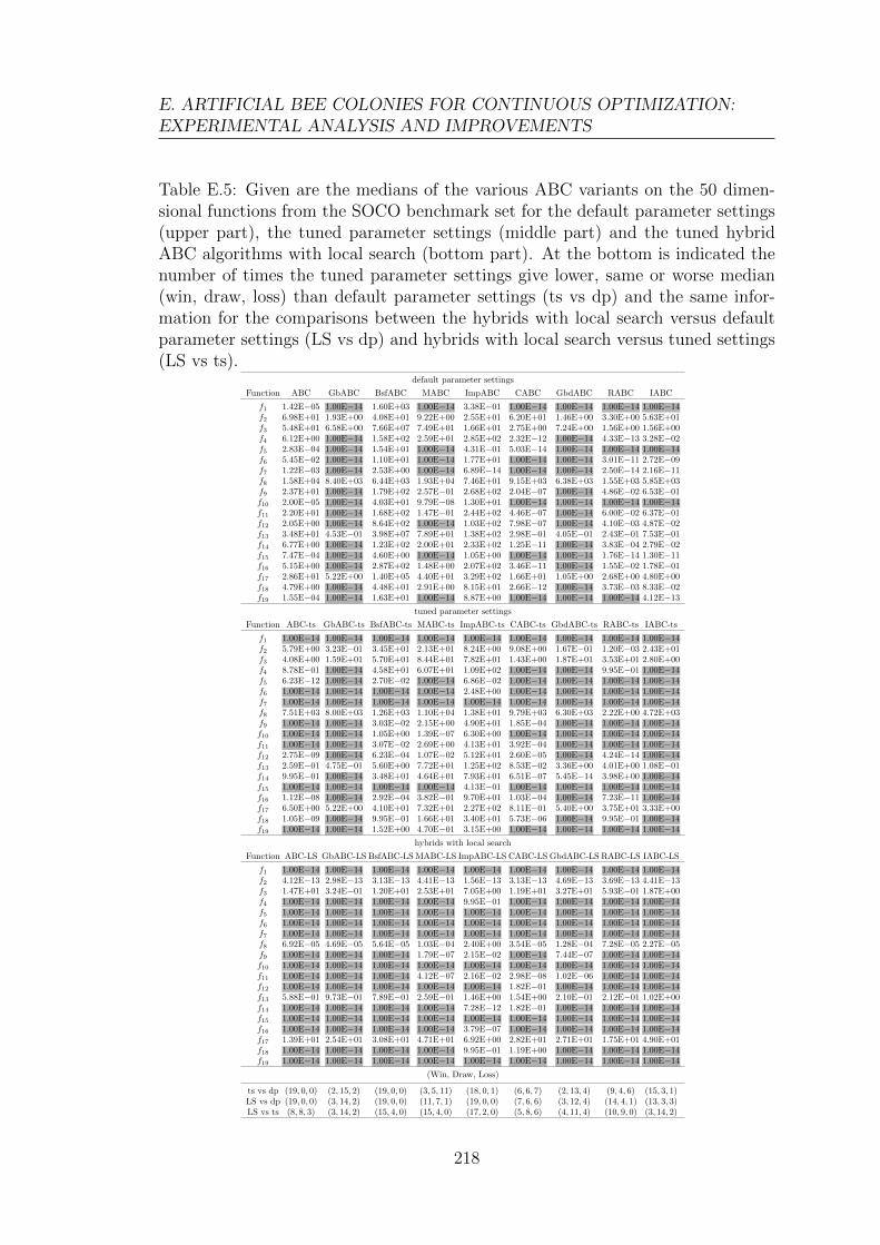
E. ARTIFICIAL BEE COLONIES FOR CONTINUOUS OPTIMIZATION:EXPERIMENTAL ANALYSIS AND IMPROVEMENTS
Table E.5: Given are the medians of the various ABC variants on the 50 dimen-sional functions from the SOCO benchmark set for the default parameter settings(upper part), the tuned parameter settings (middle part) and the tuned hybridABC algorithms with local search (bottom part). At the bottom is indicated thenumber of times the tuned parameter settings give lower, same or worse median(win, draw, loss) than default parameter settings (ts vs dp) and the same infor-mation for the comparisons between the hybrids with local search versus defaultparameter settings (LS vs dp) and hybrids with local search versus tuned settings(LS vs ts).
default parameter settings
Function ABC GbABC BsfABC MABC ImpABC CABC GbdABC RABC IABC
f1 1.42E−05 1.00E−14 1.60E+03 1.00E−14 3.38E−01 1.00E−14 1.00E−14 1.00E−14 1.00E−14f2 6.98E+01 1.93E+00 4.08E+01 9.22E+00 2.55E+01 6.20E+01 1.46E+00 3.30E+00 5.63E+01f3 5.48E+01 6.58E+00 7.66E+07 7.49E+01 1.66E+01 2.75E+00 7.24E+00 1.56E+00 1.56E+00f4 6.12E+00 1.00E−14 1.58E+02 2.59E+01 2.85E+02 2.32E−12 1.00E−14 4.33E−13 3.28E−02f5 2.83E−04 1.00E−14 1.54E+01 1.00E−14 4.31E−01 5.03E−14 1.00E−14 1.00E−14 1.00E−14f6 5.45E−02 1.00E−14 1.10E+01 1.00E−14 1.77E+01 1.00E−14 1.00E−14 3.01E−11 2.72E−09f7 1.22E−03 1.00E−14 2.53E+00 1.00E−14 6.89E−14 1.00E−14 1.00E−14 2.50E−14 2.16E−11f8 1.58E+04 8.40E+03 6.44E+03 1.93E+04 7.46E+01 9.15E+03 6.38E+03 1.55E+03 5.85E+03f9 2.37E+01 1.00E−14 1.79E+02 2.57E−01 2.68E+02 2.04E−07 1.00E−14 4.86E−02 6.53E−01f10 2.00E−05 1.00E−14 4.03E+01 9.79E−08 1.30E+01 1.00E−14 1.00E−14 1.00E−14 1.00E−14f11 2.20E+01 1.00E−14 1.68E+02 1.47E−01 2.44E+02 4.46E−07 1.00E−14 6.00E−02 6.37E−01f12 2.05E+00 1.00E−14 8.64E+02 1.00E−14 1.03E+02 7.98E−07 1.00E−14 4.10E−03 4.87E−02f13 3.48E+01 4.53E−01 3.98E+07 7.89E+01 1.38E+02 2.98E−01 4.05E−01 2.43E−01 7.53E−01f14 6.77E+00 1.00E−14 1.23E+02 2.00E+01 2.33E+02 1.25E−11 1.00E−14 3.83E−04 2.79E−02f15 7.47E−04 1.00E−14 4.60E+00 1.00E−14 1.05E+00 1.00E−14 1.00E−14 1.76E−14 1.30E−11f16 5.15E+00 1.00E−14 2.87E+02 1.48E+00 2.07E+02 3.46E−11 1.00E−14 1.55E−02 1.78E−01f17 2.86E+01 5.22E+00 1.40E+05 4.40E+01 3.29E+02 1.66E+01 1.05E+00 2.68E+00 4.80E+00f18 4.79E+00 1.00E−14 4.48E+01 2.91E+00 8.15E+01 2.66E−12 1.00E−14 3.73E−03 8.33E−02f19 1.55E−04 1.00E−14 1.63E+01 1.00E−14 8.87E+00 1.00E−14 1.00E−14 1.00E−14 4.12E−13
tuned parameter settings
Function ABC-ts GbABC-ts BsfABC-ts MABC-ts ImpABC-ts CABC-ts GbdABC-ts RABC-ts IABC-ts
f1 1.00E−14 1.00E−14 1.00E−14 1.00E−14 1.00E−14 1.00E−14 1.00E−14 1.00E−14 1.00E−14f2 5.79E+00 3.23E−01 3.45E+01 2.13E+01 8.24E+00 9.08E+00 1.67E−01 1.20E−03 2.43E+01f3 4.08E+00 1.59E+01 5.70E+01 8.44E+01 7.82E+01 1.43E+00 1.87E+01 3.53E+01 2.80E+00f4 8.78E−01 1.00E−14 4.58E+01 6.07E+01 1.09E+02 1.00E−14 1.00E−14 9.95E−01 1.00E−14f5 6.23E−12 1.00E−14 2.70E−02 1.00E−14 6.86E−02 1.00E−14 1.00E−14 1.00E−14 1.00E−14f6 1.00E−14 1.00E−14 1.00E−14 1.00E−14 2.48E+00 1.00E−14 1.00E−14 1.00E−14 1.00E−14f7 1.00E−14 1.00E−14 1.00E−14 1.00E−14 1.00E−14 1.00E−14 1.00E−14 1.00E−14 1.00E−14f8 7.51E+03 8.00E+03 1.26E+03 1.10E+04 1.38E+01 9.79E+03 6.30E+03 2.22E+00 4.72E+03f9 1.00E−14 1.00E−14 3.03E−02 2.15E+00 4.90E+01 1.85E−04 1.00E−14 1.00E−14 1.00E−14f10 1.00E−14 1.00E−14 1.05E+00 1.39E−07 6.30E+00 1.00E−14 1.00E−14 1.00E−14 1.00E−14f11 1.00E−14 1.00E−14 3.07E−02 2.69E+00 4.13E+01 3.92E−04 1.00E−14 1.00E−14 1.00E−14f12 2.75E−09 1.00E−14 6.23E−04 1.07E−02 5.12E+01 2.60E−05 1.00E−14 4.24E−14 1.00E−14f13 2.59E−01 4.75E−01 5.60E+00 7.72E+01 1.25E+02 8.53E−02 3.36E+00 4.01E+00 1.08E−01f14 9.95E−01 1.00E−14 3.48E+01 4.64E+01 7.93E+01 6.51E−07 5.45E−14 3.98E+00 1.00E−14f15 1.00E−14 1.00E−14 1.00E−14 1.00E−14 4.13E−01 1.00E−14 1.00E−14 1.00E−14 1.00E−14f16 1.12E−08 1.00E−14 2.92E−04 3.82E−01 9.70E+01 1.03E−04 1.00E−14 7.23E−11 1.00E−14f17 6.50E+00 5.22E+00 4.10E+01 7.32E+01 2.27E+02 8.11E−01 5.40E+00 3.75E+01 3.33E+00f18 1.05E−09 1.00E−14 9.95E−01 1.66E+01 3.40E+01 5.73E−06 1.00E−14 9.95E−01 1.00E−14f19 1.00E−14 1.00E−14 1.52E+00 4.70E−01 3.15E+00 1.00E−14 1.00E−14 1.00E−14 1.00E−14
hybrids with local search
Function ABC-LS GbABC-LS BsfABC-LS MABC-LS ImpABC-LS CABC-LS GbdABC-LS RABC-LS IABC-LS
f1 1.00E−14 1.00E−14 1.00E−14 1.00E−14 1.00E−14 1.00E−14 1.00E−14 1.00E−14 1.00E−14f2 4.12E−13 2.98E−13 3.13E−13 4.41E−13 1.56E−13 3.13E−13 4.69E−13 3.69E−13 4.41E−13f3 1.47E+01 3.24E−01 1.20E+01 2.53E+01 7.05E+00 1.19E+01 3.27E+01 5.93E−01 1.87E+00f4 1.00E−14 1.00E−14 1.00E−14 1.00E−14 9.95E−01 1.00E−14 1.00E−14 1.00E−14 1.00E−14f5 1.00E−14 1.00E−14 1.00E−14 1.00E−14 1.00E−14 1.00E−14 1.00E−14 1.00E−14 1.00E−14f6 1.00E−14 1.00E−14 1.00E−14 1.00E−14 1.00E−14 1.00E−14 1.00E−14 1.00E−14 1.00E−14f7 1.00E−14 1.00E−14 1.00E−14 1.00E−14 1.00E−14 1.00E−14 1.00E−14 1.00E−14 1.00E−14f8 6.92E−05 4.69E−05 5.64E−05 1.03E−04 2.40E+00 3.54E−05 1.28E−04 7.28E−05 2.27E−05f9 1.00E−14 1.00E−14 1.00E−14 1.79E−07 2.15E−02 1.00E−14 7.44E−07 1.00E−14 1.00E−14f10 1.00E−14 1.00E−14 1.00E−14 1.00E−14 1.00E−14 1.00E−14 1.00E−14 1.00E−14 1.00E−14f11 1.00E−14 1.00E−14 1.00E−14 4.12E−07 2.16E−02 2.98E−08 1.02E−06 1.00E−14 1.00E−14f12 1.00E−14 1.00E−14 1.00E−14 1.00E−14 1.00E−14 1.82E−01 1.00E−14 1.00E−14 1.00E−14f13 5.88E−01 9.73E−01 7.89E−01 2.59E−01 1.46E+00 1.54E+00 2.10E−01 2.12E−01 1.02E+00f14 1.00E−14 1.00E−14 1.00E−14 1.00E−14 7.28E−12 1.82E−01 1.00E−14 1.00E−14 1.00E−14f15 1.00E−14 1.00E−14 1.00E−14 1.00E−14 1.00E−14 1.00E−14 1.00E−14 1.00E−14 1.00E−14f16 1.00E−14 1.00E−14 1.00E−14 1.00E−14 3.79E−07 1.00E−14 1.00E−14 1.00E−14 1.00E−14f17 1.39E+01 2.54E+01 3.08E+01 4.71E+01 6.92E+00 2.82E+01 2.71E+01 1.75E+01 4.90E+01f18 1.00E−14 1.00E−14 1.00E−14 1.00E−14 9.95E−01 1.19E+00 1.00E−14 1.00E−14 1.00E−14f19 1.00E−14 1.00E−14 1.00E−14 1.00E−14 1.00E−14 1.00E−14 1.00E−14 1.00E−14 1.00E−14
(Win, Draw, Loss)
ts vs dp (19, 0, 0) (2, 15, 2) (19, 0, 0) (3, 5, 11) (18, 0, 1) (6, 6, 7) (2, 13, 4) (9, 4, 6) (15, 3, 1)LS vs dp (19, 0, 0) (3, 14, 2) (19, 0, 0) (11, 7, 1) (19, 0, 0) (7, 6, 6) (3, 12, 4) (14, 4, 1) (13, 3, 3)LS vs ts (8, 8, 3) (3, 14, 2) (15, 4, 0) (15, 4, 0) (17, 2, 0) (5, 8, 6) (4, 11, 4) (10, 9, 0) (3, 14, 2)
218

Table E.6: Given are the medians of the various ABC variants on the 100 dimen-sional functions from the SOCO benchmark set for the default parameter settings(upper part), the tuned parameter settings (middle part) and the tuned hybridABC algorithms with local search (bottom part). At the bottom is indicated thenumber of times the tuned parameter settings give lower, same or worse median(win, draw, loss) than default parameter settings (ts vs dp) and the same infor-mation for the comparisons between the hybrids with local search versus defaultparameter settings (LS vs dp) and hybrids with local search versus tuned settings(LS vs ts).
default parameter settings
Function ABC GbABC BsfABC MABC ImpABC CABC GbdABC RABC IABC
f1 5.20E−05 1.00E−14 9.10E+03 1.00E−14 1.07E+01 1.00E−14 1.00E−14 1.00E−14 1.00E−14f2 9.84E+01 1.80E+01 4.61E+01 4.09E+01 3.85E+01 9.24E+01 1.48E+01 1.59E+01 8.05E+01f3 1.80E+02 2.27E+01 6.62E+08 2.01E+02 1.76E+04 2.85E+01 4.29E+01 1.22E+01 1.27E+01f4 1.59E+01 1.00E−14 3.63E+02 1.07E+02 7.18E+02 1.70E−07 1.00E−14 2.88E−08 1.29E+00f5 1.05E−04 1.00E−14 6.78E+01 1.00E−14 1.27E+00 1.00E−14 1.00E−14 1.00E−14 1.00E−14f6 1.66E−01 1.00E−14 1.38E+01 1.00E−14 1.90E+01 1.00E−14 1.00E−14 6.24E−11 1.00E−08f7 2.77E−03 1.00E−14 6.91E+00 1.00E−14 2.29E−07 1.00E−14 1.00E−14 1.30E−13 8.03E−11f8 5.71E+04 3.36E+04 2.47E+04 9.54E+04 2.62E+03 4.07E+04 3.22E+04 1.21E+04 2.17E+04f9 5.55E+01 1.00E−14 4.12E+02 8.81E+00 5.61E+02 1.20E−07 1.00E−14 1.81E−01 1.60E+00f10 7.98E−05 1.00E−14 1.35E+02 1.05E+00 2.88E+01 1.00E−14 1.00E−14 1.00E−14 1.00E−14f11 5.65E+01 1.00E−14 4.10E+02 5.05E+00 5.69E+02 3.79E−07 1.00E−14 1.61E−01 1.77E+00f12 4.92E+00 1.00E−14 6.03E+03 1.64E−01 3.49E+02 7.58E−11 1.00E−14 1.54E−02 1.84E−01f13 8.28E+01 2.07E+00 2.80E+08 2.26E+02 3.77E+02 3.81E+00 7.34E+00 1.91E−01 1.45E+00f14 1.54E+01 1.00E−14 2.92E+02 9.01E+01 5.92E+02 7.70E−12 1.00E−14 5.02E−03 1.18E+00f15 2.07E−03 1.00E−14 1.60E+01 1.00E−14 6.07E+00 1.00E−14 1.00E−14 5.94E−14 4.94E−11f16 1.27E+01 1.00E−14 2.49E+03 2.01E+01 4.55E+02 1.94E−10 1.00E−14 5.00E−02 5.29E−01f17 6.93E+01 4.02E+00 7.73E+06 2.42E+02 6.88E+02 6.04E+00 2.95E+00 1.25E+00 8.49E+00f18 1.19E+01 1.00E−14 1.17E+02 2.63E+01 2.49E+02 6.72E−11 1.00E−14 1.49E−02 2.72E−01f19 4.98E−04 1.00E−14 7.00E+01 1.05E+00 2.41E+01 1.00E−14 1.00E−14 1.00E−14 4.18E−12
tuned parameter settings
Function ABC-ts GbABC-ts BsfABC-ts MABC-ts ImpABC-ts CABC-ts GbdABC-ts RABC-ts IABC-ts
f1 1.00E−14 1.00E−14 1.00E−14 1.00E−14 1.08E+00 1.00E−14 1.00E−14 1.00E−14 1.00E−14f2 3.67E+01 6.05E+00 4.56E+01 6.32E+01 2.73E+01 3.70E+01 3.92E+00 2.87E−01 5.33E+01f3 4.60E+01 4.31E+01 1.92E+02 1.74E+02 1.68E+02 8.95E+00 1.04E+02 2.39E+01 2.04E+01f4 2.13E+00 1.00E−14 8.16E+01 1.90E+02 4.36E+02 1.00E−14 1.00E−14 8.95E+00 9.95E−01f5 1.00E−14 1.00E−14 5.57E−02 1.00E−14 9.31E−01 1.00E−14 1.00E−14 1.00E−14 1.00E−14f6 1.00E−14 1.00E−14 1.07E−11 8.19E−08 8.96E+00 1.00E−14 1.00E−14 1.00E−14 1.00E−14f7 1.00E−14 1.00E−14 1.00E−14 1.53E−14 1.24E−14 1.00E−14 1.00E−14 1.00E−14 1.00E−14f8 3.39E+04 3.20E+04 4.98E+03 6.96E+04 1.18E+03 3.90E+04 2.82E+04 2.27E+02 1.90E+04f9 4.18E−07 1.00E−14 1.39E+01 1.66E+02 3.43E+02 8.53E−04 1.00E−14 1.00E−14 1.00E−14f10 1.00E−14 1.00E−14 4.20E+00 2.10E+00 2.10E+01 1.00E−14 1.00E−14 1.00E−14 1.00E−14f11 6.91E−07 1.00E−14 2.29E−01 1.54E+02 3.51E+02 9.34E−04 1.00E−14 1.00E−14 1.00E−14f12 1.30E−08 1.00E−14 3.29E−05 1.37E+00 1.90E+02 9.58E−05 1.00E−14 3.07E−11 1.00E−14f13 2.05E+00 6.70E+00 6.96E+01 2.09E+02 3.48E+02 8.28E−01 2.34E+01 2.71E+01 9.38E−01f14 1.99E+00 1.00E−14 9.45E+01 1.42E+02 3.23E+02 4.20E−06 3.14E−11 6.96E+00 9.95E−01f15 1.00E−14 1.00E−14 1.00E−14 1.06E−14 3.15E+00 1.00E−14 1.00E−14 1.00E−14 1.00E−14f16 1.35E−08 1.00E−14 1.08E−02 2.13E+01 3.44E+02 2.24E−04 1.00E−14 3.94E−09 1.00E−14f17 1.48E+01 1.52E+01 2.97E+01 3.30E+02 5.93E+02 2.41E+00 1.39E+01 2.38E+01 6.30E+00f18 9.95E−01 1.00E−14 5.18E+01 9.57E+01 1.18E+02 1.11E−05 1.00E−14 2.98E+00 1.00E−14f19 1.00E−14 1.00E−14 7.35E+00 3.15E+00 1.78E+01 1.00E−14 1.00E−14 1.00E−14 1.00E−14
hybrids with local search
Function ABC-LS GbABC-LS BsfABC-LS MABC-LS ImpABC-LS CABC-LS GbdABC-LS RABC-LS IABC-LS
f1 1.00E−14 1.00E−14 1.00E−14 1.00E−14 1.00E−14 1.00E−14 1.00E−14 1.00E−14 1.00E−14f2 6.45E−12 3.62E−12 5.05E−12 2.58E−11 2.59E−12 7.39E−12 4.09E−11 3.60E−12 2.98E−12f3 5.63E+01 2.86E+01 4.25E+01 3.97E+01 5.38E+01 8.64E+01 1.46E+02 5.06E+01 3.83E+01f4 1.00E−14 1.00E−14 1.00E−14 1.00E−14 1.00E−14 1.00E−14 1.00E−14 1.00E−14 1.00E−14f5 1.00E−14 1.00E−14 1.00E−14 1.00E−14 1.00E−14 1.00E−14 1.00E−14 1.00E−14 1.00E−14f6 1.00E−14 1.00E−14 1.00E−14 1.00E−14 1.00E−14 1.00E−14 1.00E−14 1.00E−14 1.00E−14f7 1.00E−14 1.00E−14 1.00E−14 1.00E−14 1.00E−14 1.00E−14 1.00E−14 1.00E−14 1.00E−14f8 1.79E+00 1.42E+00 1.53E+00 2.44E+00 4.88E+02 4.45E−01 2.56E+00 1.72E+00 1.22E+00f9 1.00E−14 1.00E−14 1.00E−14 1.21E−06 2.72E−01 1.14E−07 2.94E−06 1.00E−14 1.00E−14f10 1.00E−14 1.00E−14 1.00E−14 1.00E−14 1.00E−14 1.00E−14 1.00E−14 1.00E−14 1.00E−14f11 4.48E−08 1.00E−14 2.11E−08 1.49E−06 1.09E+00 3.76E−07 2.38E−06 1.00E−14 1.00E−14f12 1.00E−14 1.00E−14 1.00E−14 1.00E−14 8.10E−06 1.00E−14 1.00E−14 1.00E−14 1.00E−14f13 1.17E+01 2.29E+00 1.15E+01 1.13E+01 8.91E+00 5.56E+00 7.38E+00 5.60E+00 2.00E+01f14 1.00E−14 1.00E−14 1.00E−14 1.00E−14 5.55E−04 1.00E−14 1.00E−14 1.00E−14 1.00E−14f15 1.00E−14 1.00E−14 1.00E−14 1.00E−14 1.00E−14 1.00E−14 1.00E−14 1.00E−14 1.00E−14f16 1.00E−14 1.00E−14 1.00E−14 1.00E−14 2.74E−04 1.00E−14 1.00E−14 1.00E−14 1.00E−14f17 2.56E+01 1.98E+01 3.01E+01 1.57E+01 2.81E+01 3.03E+01 2.01E+01 2.78E+01 2.23E+01f18 1.00E−14 1.00E−14 1.00E−14 1.00E−14 7.69E−01 1.00E−14 1.00E−14 1.00E−14 1.00E−14f19 1.00E−14 1.00E−14 1.00E−14 1.00E−14 1.00E−14 1.00E−14 1.00E−14 1.00E−14 1.00E−14
(Win, Draw, Loss)
ts vs dp (19, 0, 0) (2, 14, 3) (19, 0, 0) (3, 2, 14) (19, 0, 0) (6, 7, 6) (2, 13, 4) (9, 4, 6) (15, 3, 1)LS vs dp (19, 0, 0) (2, 14, 3) (19, 0, 0) (14, 5, 0) (19, 0, 0) (9, 7, 3) (2, 12, 5) (12, 4, 3) (13, 3, 3)LS vs ts (9, 7, 3) (4, 14, 1) (15, 3, 1) (17, 2, 0) (19, 0, 0) (8, 8, 3) (4, 11, 4) (8, 9, 2) (4, 12, 3)
219

E. ARTIFICIAL BEE COLONIES FOR CONTINUOUS OPTIMIZATION:EXPERIMENTAL ANALYSIS AND IMPROVEMENTS
Table E.7: Given are the medians of the various ABC variants on the 500 dimen-sional functions from the SOCO benchmark set for the default parameter settings(upper part), the tuned parameter settings (middle part) and the tuned hybridABC algorithms with local search (bottom part). At the bottom is indicated thenumber of times the tuned parameter settings give lower, same or worse median(win, draw, loss) than default parameter settings (ts vs dp) and the same infor-mation for the comparisons between the hybrids with local search versus defaultparameter settings (LS vs dp) and hybrids with local search versus tuned settings(LS vs ts).
default parameter settings
Function ABC GbABC BsfABC MABC ImpABC CABC GbdABC RABC IABC
f1 4.68E−04 1.00E−14 1.49E+05 3.78E−02 4.19E+03 1.00E−14 1.00E−14 1.00E−14 1.00E−14f2 1.49E+02 8.46E+01 4.95E+01 1.21E+02 4.87E+01 1.44E+02 8.28E+01 8.09E+01 1.12E+02f3 5.72E+02 2.99E+01 3.26E+10 2.95E+03 4.14E+08 1.40E+01 7.94E+01 1.95E+01 1.64E+01f4 1.19E+02 1.00E−14 2.38E+03 1.49E+03 4.10E+03 1.99E+00 1.00E−14 3.08E+00 1.74E+01f5 3.17E−04 1.00E−14 1.20E+03 7.63E−03 2.26E+01 1.00E−14 1.00E−14 1.00E−14 1.00E−14f6 7.38E−01 1.00E−14 1.74E+01 2.68E+00 1.93E+01 1.00E−14 1.00E−14 4.31E−10 9.15E−08f7 1.74E−02 1.00E−14 5.25E+01 5.46E−06 1.02E+02 1.00E−14 1.00E−14 2.98E−12 2.35E−09f8 8.66E+05 5.56E+05 3.63E+05 1.87E+06 1.57E+05 6.79E+05 5.25E+05 4.14E+05 2.89E+05f9 3.84E+02 1.00E−14 2.49E+03 2.80E+03 3.13E+03 1.70E−07 1.00E−14 1.15E+00 1.29E+01f10 1.40E−03 1.00E−14 1.79E+03 2.63E+01 1.18E+02 1.00E−14 1.00E−14 1.00E−14 1.00E−14f11 3.94E+02 1.00E−14 2.48E+03 2.73E+03 3.16E+03 1.47E−07 1.00E−14 1.17E+00 1.33E+01f12 4.68E+01 1.00E−14 1.12E+05 6.63E+02 3.68E+03 8.83E−10 1.00E−14 1.89E−01 1.73E+00f13 5.34E+02 4.55E+01 2.03E+10 2.14E+03 2.16E+08 1.94E+01 1.13E+02 6.30E+00 2.34E+01f14 1.08E+02 1.03E+00 1.89E+03 1.18E+03 3.13E+03 1.99E+00 9.95E−01 2.17E+00 1.32E+01f15 9.30E−03 1.00E−14 1.77E+02 3.62E+00 1.79E+02 1.00E−14 1.00E−14 1.45E−12 1.31E−09f16 1.07E+02 1.00E−14 6.45E+04 1.45E+03 3.35E+03 5.58E−09 1.00E−14 4.49E−01 4.12E+00f17 2.17E+02 1.06E+00 3.07E+09 3.26E+03 2.79E+06 4.00E+00 1.42E+00 2.92E+00 1.80E+01f18 8.43E+01 2.28E−03 8.62E+02 7.88E+02 1.37E+03 3.03E−02 9.95E−01 2.66E−01 6.01E+00f19 2.95E−03 1.00E−14 2.51E+02 1.99E+01 1.70E+02 1.00E−14 1.00E−14 1.79E−13 1.63E−10
tuned parameter settings
Function ABC-ts GbABC-ts BsfABC-ts MABC-ts ImpABC-ts CABC-ts GbdABC-ts RABC-ts IABC-ts
f1 1.00E−14 1.00E−14 1.00E−14 4.57E+00 3.09E+03 1.00E−14 1.00E−14 1.00E−14 1.00E−14f2 1.08E+02 6.72E+01 4.94E+01 1.35E+02 4.71E+01 1.02E+02 5.83E+01 2.21E+01 9.61E+01f3 3.86E+01 2.57E+01 4.41E+02 4.58E+04 2.46E+08 2.46E+00 2.21E+02 5.07E+01 9.79E+00f4 2.29E+01 1.00E−14 9.40E+02 2.08E+03 3.56E+03 3.43E−08 1.13E+00 7.56E+01 2.98E+00f5 1.00E−14 1.00E−14 3.48E−10 7.43E−01 2.24E+01 1.00E−14 4.01E−04 1.00E−14 1.00E−14f6 1.00E−14 1.00E−14 1.01E+00 1.98E+01 1.91E+01 1.00E−14 1.00E−14 1.00E−14 1.00E−14f7 1.00E−14 1.00E−14 1.00E−14 1.26E−02 1.34E+01 1.00E−14 1.00E−14 1.00E−14 1.00E−14f8 5.43E+05 5.27E+05 9.15E+04 1.23E+06 8.50E+04 5.06E+05 5.06E+05 1.12E+05 3.20E+05f9 3.13E−06 1.00E−14 3.04E+02 3.48E+03 2.96E+03 6.63E−03 1.00E−14 7.72E+00 1.00E−14f10 1.00E−14 1.00E−14 4.20E+01 4.20E+01 1.30E+02 1.00E−14 1.00E−14 1.00E−14 1.00E−14f11 1.07E−02 1.00E−14 1.54E+02 3.47E+03 2.94E+03 6.29E−03 1.00E−14 8.96E+00 1.00E−14f12 2.89E−07 1.00E−14 6.28E−02 9.64E+02 2.68E+03 7.45E−04 2.26E−01 1.10E−01 1.00E−14f13 3.95E+01 6.83E+01 6.59E+02 2.75E+03 7.09E+07 7.86E+00 1.88E+02 5.48E+01 4.14E+00f14 1.69E+01 9.95E−01 6.42E+02 1.66E+03 2.75E+03 8.86E−05 1.35E+00 4.88E+01 9.95E−01f15 1.00E−14 1.00E−14 1.05E+00 7.54E+00 6.15E+01 1.00E−14 1.00E−14 1.00E−14 1.00E−14f16 1.19E−06 1.00E−14 1.84E−01 1.97E+03 2.97E+03 3.01E−03 1.08E−01 3.03E−02 1.00E−14f17 1.02E+00 1.29E+01 1.15E+02 3.60E+03 4.35E+03 5.99E−01 2.30E+01 3.20E+01 1.49E+00f18 5.97E+00 7.02E−07 5.46E+02 9.39E+02 1.21E+03 1.98E−04 1.97E−06 1.79E+01 1.00E−14f19 1.00E−14 1.00E−14 2.10E+00 2.52E+01 1.17E+02 1.00E−14 1.00E−14 1.00E−14 1.00E−14
hybrids with local search
Function ABC-LS GbABC-LS BsfABC-LS MABC-LS ImpABC-LS CABC-LS GbdABC-LS RABC-LS IABC-LS
f1 1.00E−14 1.00E−14 1.00E−14 1.00E−14 1.00E−14 1.00E−14 1.00E−14 1.00E−14 1.00E−14f2 1.82E−02 1.18E−02 1.31E−02 1.69E−02 7.89E−03 1.04E−02 1.69E−02 1.80E−02 1.09E−02f3 6.63E+00 2.21E+01 9.05E+00 1.22E+01 4.62E+00 9.84E+00 1.26E+01 2.12E+01 2.52E+01f4 1.00E−14 1.00E−14 1.00E−14 1.00E−14 1.00E−14 1.00E−14 1.00E−14 1.00E−14 1.00E−14f5 1.00E−14 1.00E−14 1.00E−14 1.00E−14 1.00E−14 1.00E−14 1.00E−14 1.00E−14 1.00E−14f6 1.00E−14 1.00E−14 1.00E−14 1.00E−14 1.00E−14 1.00E−14 1.00E−14 1.00E−14 1.00E−14f7 1.00E−14 1.00E−14 1.00E−14 3.57E−14 1.00E−14 1.00E−14 7.52E−14 1.00E−14 1.00E−14f8 3.69E+04 3.23E+04 3.83E+04 3.78E+04 1.15E+05 1.06E+04 3.70E+04 3.59E+04 3.15E+04f9 4.23E−05 2.73E−06 6.40E−06 1.49E−05 4.46E+00 4.10E−06 2.76E−05 1.72E−06 8.16E−06f10 1.00E−14 1.00E−14 1.00E−14 1.00E−14 1.00E−14 1.00E−14 1.00E−14 1.00E−14 1.00E−14f11 1.19E−05 2.38E−05 1.09E−05 1.57E−05 3.71E+00 6.77E−06 2.98E−05 1.86E−05 5.10E−06f12 1.00E−14 1.00E−14 1.00E−14 1.00E−14 1.08E−01 1.00E−14 1.00E−14 1.00E−14 1.00E−14f13 3.93E+01 4.05E+01 6.60E+01 6.62E+01 1.89E+01 4.63E+01 4.26E+01 5.60E+01 2.16E+01f14 1.00E−14 1.00E−14 1.00E−14 1.00E−14 1.10E−01 6.60E−05 1.00E−14 1.00E−14 1.00E−14f15 1.00E−14 1.00E−14 1.00E−14 1.00E−14 1.00E−14 1.00E−14 4.16E−14 1.00E−14 1.00E−14f16 1.00E−14 1.00E−14 1.00E−14 1.00E−14 5.95E−01 1.34E+00 1.00E−14 1.00E−14 1.00E−14f17 1.75E+01 1.32E+01 9.70E+00 2.00E+01 2.35E+01 1.87E+01 1.21E+01 8.51E+00 1.74E+01f18 1.00E−14 1.00E−14 1.00E−14 1.00E−14 1.10E+01 1.27E+01 1.00E−14 1.00E−14 1.00E−14f19 1.00E−14 1.00E−14 1.00E−14 1.00E−14 1.00E−14 1.00E−14 1.00E−14 1.00E−14 1.00E−14
(Win, Draw, Loss)
ts vs dp (19, 0, 0) (5, 12, 2) (19, 0, 0) (1, 0, 18) (18, 0, 1) (8, 7, 4) (3, 8, 8) (8, 3, 8) (15, 3, 1)LS vs dp (19, 0, 0) (6, 10, 3) (19, 0, 0) (19, 0, 0) (19, 0, 0) (6, 7, 6) (6, 8, 5) (13, 3, 3) (15, 3, 1)LS vs ts (10, 7, 2) (6, 10, 3) (17, 2, 0) (19, 0, 0) (18, 0, 1) (7, 7, 5) (11, 3, 4) (11, 7, 2) (4, 10, 5)
220

Bibliography
K. Abhishek, S. Leyffer, and J. T. Linderoth. Modeling without categorical vari-
ables: a mixed-integer nonlinear program for the optimization of thermal insu-
lation systems. Optimization and Engineering, 11(2):185–212, 2010.
A. Abraham, R. K. Jatoth, and A. Rajasekhar. Hybrid differential artificial bee
colony algorithm. Journal of Computational and Theoretical Nanoscience, 9(2):
249–257, 2012.
M. A. Abramson. Pattern search algorithms for mixed variable general constrained
optimization problems. PhD thesis, Ecole Polytechnique de Montreal, Canada,
2002.
M. A. Abramson. Mixed variable optimization of a load-bearing thermal insulation
system using a filter pattern search algorithm. Optimization and Engineering,
5(2):157–177, 2004.
M. A. Abramson, C. Audet, J. W. Chrissis, and J. G. Walston. Mesh adaptive
direct search algorithms for mixed variable optimization. Optimization Letters,
3(1):35–47, 2009.
D. H. Ackley. A connectionist machine for genetic hillclimbing. Kluwer, Boston,
1987.
B. Adenso-Diaz and M. Laguna. Fine-tuning of algorithms using fractional exper-
imental designs and local search. Operations Research, 54:99–114, 2006.
B. Akay and D. Karaboga. Artificial bee colony algorithm for large-scale problems
and engineering design optimization. Journal of Intelligent Manufacturing. In
press.
B. Akay and D. Karaboga. Parameter tuning for the artificial bee colony algorithm.
In N. T. Nguyen, R. Kowalczyk, and S.-M. Chen, editors, Proceedings of the
1st International Conference on Computational Collective Intelligence. Semantic
221

BIBLIOGRAPHY
Web, Social Networks and Multiagent Systems, ICCCI’09., LNCS 5796, pages
608–619. Springer Verlag, Heidelberg, Germany, 2009.
B. Akay and D. Karaboga. A modified artificial bee colony algorithm for real-
parameter optimization. Information Sciences, 192:120–142, 2012.
M. S. Alam, M. W. Ul Kabir, and M. M. Islam. Self-adaptation of mutation step
size in artificial bee colony algorithm for continuous function optimization. In
Proceedings of International Conference on Computer and Information Technol-
ogy, ICCIT’10, pages 69–74. IEEE Press, Piscataway, NJ, 2010.
B. Alatas. Chaotic bee colony algorithms for global numerical optimization. Expert
Systems with Applications, 37(8):5682–5687, 2010.
N. Andreasson, A. Evggrafov, and M. Patriksson. An introduction to continuous
optimization. Lightning Source Incorporated, 2005.
C. Audet and J. E. Dennis, Jr. Pattern search algorithms for mixed variable
programming. SIAM Journal on Optimization, 11(3):573–594, 2001.
C. Audet and J. E. Dennis Jr. Mesh adaptive direct search algorithms for con-
strained optimization. SIAM Journal on optimization, 17(1):188–217, 2006.
A. Auger and N. Hansen. A restart CMA evolution strategy with increasing pop-
ulation size. In Proceeding of IEEE Congress on Evolutionary Computation,
CEC’05, pages 1769–1776, Piscataway, NJ, USA, 2005. IEEE Press.
D. Aydın, T. Liao, M. A. Montes de Oca, and T. Stutzle. Improving performance
via population growth and local search: The case of the artificial bee colony
algorithm. In J.-K. Hao, P. Legrand, P. Collet, N. Monmarche, E. Lutton, and
M. Schoenauer, editors, Artificial Evolution, LNCS 7401, pages 85–96. Springer
Verlag, Heidelberg, Germany, 2012.
P. Balaprakash, M. Birattari, and T. Stutzle. Improvement strategies for the F-
Race algorithm: sampling design and iterative refinement. In Bartz-Beielstein
et al., editors, Proceedings of Conference on Hybrid Metaheuristics, LNCS 4771,
pages 108–122. Springer, Heidelberg, Germany, 2007.
A. Banharnsakun, T. Achalakul, and B. Sirinaovakul. The best-so-far selection in
artificial bee colony algorithm. Applied Soft Computing, 11(2):2888–2901, 2011.
222

BIBLIOGRAPHY
T. Bartz-Beielstein. Experimental Research in Evolutionary Computation: the New
Experimentalism. Springer, 2006.
R. Battiti. First-and second-order methods for learning: between steepest descent
and newton’s method. Neural computation, 4(2):141–166, 1992.
H. Bersini, M. Dorigo, S. Langerman, G. Seront, and L. Gambardella. Results
of the first international contest on evolutionary optimisation (1st ICEO). In
Proceedings of IEEE International Conference on Evolutionary Computation,
ICEC’96, pages 611–615, Piscataway, NJ, 1996. IEEE Press.
H.-G. Beyer and H.-P. Schwefel. Evolution strategies - a comprehensive introduc-
tion. Natural Computing, 1:3–52, 2002.
G. Bilchev and I. Parmee. The Ant Colony Metaphor for Searching Continuous De-
sign Spaces. In T. Fogarty, editor, AISB Workshop on Evolutionary Computing,
pages 25–39. Springer-Verlag, 1995.
M. Birattari. Tuning Metaheuristics: A Machine Learning Perspective. Springer,
Berlin, Germany, 1st ed. 2005. 2nd printing edition, 2009.
M. Birattari, T. Stutzle, L. Paquete, and K. Varrentrapp. A racing algorithm
for configuring metaheuristics. In Proceedings of the Genetic and Evolutionary
Computation Conference, GECCO’02, pages 11–18, San Francisco, CA, USA,
2002. Morgan Kaufmann.
M. Birattari, Z. Yuan, P. Balaprakash, and T. Stutzle. F-Race and iterated F-
Race: An overview. In Bartz-Beielstein et al., editors, Experimental Methods
for the Analysis of Optimization Algorithms, pages 311–336. Springer, Berlin,
Germany, 2010.
B. Bischl, O. Mersmann, H. Trautmann, and M. Preuß. Algorithm selection based
on exploratory landscape analysis and cost-sensitive learning. In Proceedings of
Genetic and Evolutionary Computation Conference, GECCO’12, pages 313–320,
New York, NY, USA, 2012. ACM.
G. E. Box. Evolutionary operation: A method for increasing industrial productiv-
ity. Applied Statistics, pages 81–101, 1957.
D. Brockhoff, A. Auger, and N. Hansen. On the impact of active covariance
matrix adaptation in the CMA-ES with mirrored mutations and small initial
223

BIBLIOGRAPHY
population size on the noiseless BBOB testbed. In Proceedings of the Genetic and
Evolutionary Computation Conference, GECCO’12 (Companion), pages 291–
296, New York, NY, USA, 2012. ACM.
S. Brooks. A discussion of random methods for seeking maxima. Operations
Research, 6(2):244–251, 1958.
M. R. Bussieck and A. Pruessner. Mixed-integer nonlinear programming.
SIAG/OPT Newsletter: Views & News, 14(1):19–22, 2003.
Y. Cao and Q. Wu. Mechanical design optimization by mixed-variable evolu-
tionary programming. In Proceedings of the IEEE Conference on Evolutionary
Computation, pages 443–446. IEEE Press, Piscataway, NJ, 1997.
J. Chen and Y. Tsao. Optimal design of machine elements using genetic algorithms.
Journal of the Chinese Society of Mechanical Engineers, 14(2):193–199, 1993.
M. Clerc and J. Kennedy. The particle swarm-explosion, stability, and convergence
in a multidimensional complex space. IEEE Transactions on Evolutionary Com-
putation, 6(1):58–73, 2002.
C. A. Coello Coello. Use of a self-adaptive penalty approach for engineering opti-
mization problems. Computers in Industry, 41(2):113–127, 2000.
C. A. Coello Coello and R. L. Becerra. Efficient evolutionary optimization through
the use of a cultural algorithm. Engineering Optimization, 36(2):219–236, 2004.
C. A. Coello Coello and E. Mezura Montes. Constraint-handling in genetic al-
gorithms through the use of dominance-based tournament selection. Advanced
Engineering Informatics, 16(3):193–203, 2002.
A. R. Conn, N. I. Gould, and P. L. Toint. Trust region methods, volume 1. SIAM,
1987.
A. R. Conn, K. Scheinberg, and L. N. Vicente. Introduction to derivative-free
optimization. Society for Industrial and Applied Mathematics, 2009.
W. J. Conover. Practical Nonparametric Statistics. John Wiley & Sons, New York,
NY, USA, 1998.
G. B. Dantzig and M. N. Thapa. Linear Programming 1: Introduction. Springer,
1997.
224

BIBLIOGRAPHY
G. B. Dantzig and M. N. Thapa. Linear Programming 2: Theory and Extensions.
Springer, 2003.
S. Das, A. Abraham, U. K. Chakraborty, and A. Konar. Differential evolution using
a neighborhood-based mutation operator. IEEE Transactions on Evolutionary
Computation, 13(3):526–553, 2009.
S. Das, P. N. Suganthan, and C. A. Coello Coello. Guest editorial special issue on
differential evolution. IEEE Transactions on Evolutionary Computation, 15(1):
1–3, 2011.
D. Datta and J. Figueira. A real-integer-discrete-coded differential evolution algo-
rithm: A preliminary study. In P. Cowling and P. Merz, editors, Evolutionary
Computation in Combinatorial Optimization, LNCS 6022, pages 35–46. Springer
Verlag, Heidelberg, Germany, 2010.
W. C. Davidon. Variable metric method for minimization. SIAM Journal on
Optimization, 1(1):1–17, 1991.
C. De Boor and A. Ron. On multivariate polynomial interpolation. Constructive
Approximation, 6(3):287–302, 1990.
K. Deb and M. Goyal. A combined genetic adaptive search (GeneAS) for engi-
neering design. Computer Science and Informatics, 26:30–45, 1996.
K. Deb and M. Goyal. A flexible optimization procedure for mechanical component
design based on genetic adaptive search. Journal of Mechanical Design, 120(2):
162–164, 1998.
J. E. Dennis, Jr and V. Torczon. Direct search methods on parallel machines.
SIAM Journal on Optimization, 1(4):448–474, 1991.
G. G. Dimopoulos. Mixed-variable engineering optimization based on evolutionary
and social metaphors. Computer Methods in Applied Mechanics and Engineer-
ing, 196(4-6):803 – 817, 2007.
K. Diwold, A. Aderhold, A. Scheidler, and M. Middendorf. Performance evalua-
tion of artificial bee colony optimization and new selection schemes. Memetic
Computing, 3(3):149–162, 2011a.
K. Diwold, M. Beekman, and M. Middendorf. Honeybee optimisation-an overview
and a new bee inspired optimisation scheme. In B. K. Panigrahi, Y. Shi, and
225

BIBLIOGRAPHY
M.-H. Lim, editors, Handbook of Swarm Intelligence-Concepts, Principles and
Application, volume 8 of Adaptation, Learning, and Optimization, pages 295–
328. Springer Verlag, Berlin, Germany, 2011b.
M. Dorigo and G. Di Caro. The Ant Colony Optimization meta-heuristic. In
D. Corne, M. Dorigo, and F. Glover, editors, New Ideas in Optimization, pages
11–32. McGraw Hill, London, UK, 1999.
M. Dorigo and T. Stutzle. Ant Colony Optimization. MIT Press, Cambridge, MA,
2004.
M. Dorigo, V. Maniezzo, and A. Colorni. Positive feedback as a search strategy.
Technical Report 91-016, Dipartimento di Elettronica, Politecnico di Milano,
Italy, 1991.
M. Dorigo, V. Maniezzo, and A. Colorni. Ant System: Optimization by a colony
of cooperating agents. IEEE Transactions on Systems, Man, and Cybernetics –
Part B, 26(1):29–41, 1996.
B. Dorronsoro and P. Bouvry. Improving classical and decentralized differential
evolution with new mutation operator and population topologies. IEEE Trans-
actions on Evolutionary Computation, 15(1):67–98, 2011.
J. Dreo and P. Siarry. Continuous interacting ant colony algorithm based on dense
heterarchy. Future Generation Computer Systems, 20(5):841–856, 2004.
J. Dubois-Lacoste, M. Lopez-Ibanez, and T. Stutzle. Automatic configura-
tion of state-of-the-art multi-objective optimizers using the TP+PLS frame-
work. In Proceedings of the Genetic and Evolutionary Computation Conference,
GECCO’11, pages 2019–2026, New York, NY, USA, 2011. ACM.
A. Eiben and T. Back. Empirical investigation of multiparent recombination op-
erators in evolution strategies. Evolutionary Computation, 5(3):347–365, 1997.
M. El-Abd. Opposition-based artificial bee colony algorithm. In N. Krasnogor
and P. L. Lanzi, editors, Proceedings of Genetic and Evolutionary Computation
Conference, GECCO’11, pages 109–116. ACM, 2011a.
M. El-Abd. A hybrid ABC-SPSO algorithm for continuous function optimization.
In Proceedings of IEEE Symposium on Swarm Intelligence, pages 1–6. IEEE
Press, Piscataway, NJ, 2011b.
226

BIBLIOGRAPHY
M. Epitropakis, D. Tasoulis, N. Pavlidis, V. Plagianakos, and M. Vrahatis. Enhanc-
ing differential evolution utilizing proximity-based mutation operators. IEEE
Transactions on Evolutionary Computation, 15(1):99–119, 2011.
L. J. Eshelman and J. D. Schaffer. Real-coded genetic algorithms and interval-
schemata. In D. L. Whitley, editor, Foundation of Genetic Algorithms 2, pages
187–202, San Mateo, CA, 1993. Morgan Kaufmann.
I. Fister, I. Fister Jr., J. Brest, and V. Zumer. Memetic artificial bee colony
algorithm for large-scale global optimization. In IEEE Congress on Evolutionary
Computation, CEC’12, pages 1–8. IEEE Press, Piscataway, NJ, 2012.
J.-F. Fu, R. Fenton, and W. Cleghorn. A mixed integer-discrete-continuous pro-
gramming method and its application to engineering design optimization. En-
gineering Optimization, 17(4):263–280, 1991.
L. Gao and A. Hailu. Comprehensive learning particle swarm optimizer for con-
strained mixed-variable optimization problems. International Journal of Com-
putational Intelligence Systems, 3(6):832–842, 2010.
W. Gao and S. Liu. Improved artificial bee colony algorithm for global optimiza-
tion. Information Processing Letters, 111(17):871–882, 2011.
W. Gao, S. Liu, and L. Huang. A global best artificial bee colony algorithm for
global optimization. Journal of Computational and Applied Mathematics, 236
(11):2741–2753, 2012.
S. Ghosh, S. Das, S. Roy, S. K. Minhazul Islam, and P. N. Suganthan. A differ-
ential covariance matrix adaptation evolutionary algorithm for real parameter
optimization. Information Science, 182(1):199–219, 2012.
J. Gimmler. Metaheuristiken zur kontiuierlichen, globalen optimierung. Master’s
thesis, Computer Science Department, TU, Darmstadt, Germany, 2005.
J. Gimmler, T. Stutzle, and T. E. Exner. Hybrid particle swarm optimization:
An examination of the influence of iterative improvement algorithms on perfor-
mance. In M. Dorigo et al., editors, Proceedings of International Conference on
Ant Colony Optimization and Swarm Intelligence, ANTS’06, LNCS 4150, pages
436–443. Springer, Heidelberg, Germany, 2006.
D. E. Goldberg. Genetic Algorithms in Search, Optimization and Machine Learn-
ing. Addison-Wesley, Boston, MA, USA, 1989.
227

BIBLIOGRAPHY
C. P. Gomes and B. Selman. Algorithm portfolios. Artificial Intelligence, 126(12):
4–62, 2001.
T. Gonen. Electric power distribution system engineering. McGraw-Hill, New
York, USA, 1986.
A. Griewank. Generalized descent for global optimization. Journal of optimization
theory and applications, 34(1):11–39, 1981.
I. Griva, S. G. Nash, and A. Sofer. Linear and nonlinear optimization. Society for
Industrial and Applied Mathematics, 2009.
M. Guntsch and M. Middendorf. A population based approach for ACO. In
S. Cagnoni et al., editors, Proceedings of EvoWorkshops 2002: EvoCOP,
EvoIASP, EvoSTim, volume 2279 of LNCS, pages 71–80. Springer, Berlin, Ger-
many, 2002.
C. Guo, J. Hu, B. Ye, and Y. Cao. Swarm intelligence for mixed-variable design
optimization. Journal of Zhejiang University Science, 5(7):851–860, 2004.
P. Guo, W. Cheng, and J. Liang. Global artificial bee colony search algorithm for
numerical function optimization. In Proceedings of International Conference on
Natural Computation, volume 3, pages 1280–1283. IEEE Press, Piscataway, NJ,
2011.
N. Hansen. Benchmarking a BI-population CMA-ES on the BBOB-2009 function
testbed. In Proceedings of the Genetic and Evolutionary Computation Confer-
ence, GECCO’12 (Companion), pages 2389–2396, New York, NY, USA, 2009.
ACM.
N. Hansen. The CMA evolution strategy: A tutorial, 2010. Online: http://www.
lri. fr/hansen/cmatutorial. pdf.
N. Hansen and A. Ostermeier. Adapting arbitrary normal mutation distributions
in evolution strategies: The covariance matrix adaptation. In Proceedings of
IEEE International Conference on Evolutionary Computation, CEC’96, pages
312–317, Piscataway, NJ, 1996. IEEE Press.
N. Hansen and A. Ostermeier. Completely derandomized self-adaptation in evo-
lution strategies. Evolutionary Computation, 9(2):159–195, 2001.
228

BIBLIOGRAPHY
N. Hansen, S. Muller, and P. Koumoutsakos. Reducing the time complexity of the
derandomized evolution strategy with covariance matrix adaptation (CMA-ES).
Evolutionary Computation, 11(1):1–18, 2003.
N. Hansen, S. Finck, R. Ros, and A. Auger. Real-parameter black-box optimization
benchmarking 2009: Noiseless functions definitions. 2009a. Technical Report
RR-6829, INRIA.
N. Hansen, S. Finck, R. Ros, and A. Auger. Real-parameter black-box optimization
benchmarking 2009: Noisy functions definitions. Technical Report Research
Report RR-6869, INRIA, 2009b.
N. Hansen, A. S. P. Niederberger, L. Guzzella, and P. Koumoutsakos. A method for
handling uncertainty in evolutionary optimization with an application to feed-
back control of combustion. IEEE Transactions on Evolutionary Computation,
13(1):180–197, 2009c.
Q. He and L. Wang. An effective co-evolutionary particle swarm optimization for
constrained engineering design problems. Engineering Applications of Artificial
Intelligence, 20(1):89–99, 2007a.
Q. He and L. Wang. A hybrid particle swarm optimization with a feasibility-based
rule for constrained optimization. Applied Mathematics and Computation, 186
(2):1407–1422, 2007b.
F. Herrera and M. Lozano. Two-loop real-coded genetic algorithms with adaptive
control of mutation step sizes. Applied Intelligence, 13(3):187–204, 2000.
F. Herrera, M. Lozano, and J. Verdegay. Tackling real-coded genetic algorithms:
Operators and tools for behavioural analysis. Artificial Intelligence Review, 12:
265–319, 1998.
F. Herrera, M. Lozano, and A. Sanchez. A taxonomy for the crossover operator for
real-coded genetic algorithms: An experimental study. International Journal of
Intelligent Systems, 18(3):309–338, 2003.
F. Herrera, M. Lozano, and A. Sanchez. Hybrid crossover operators for real-coded
genetic algorithms: an experimental study. Soft Computing, 9(4):280–298, 2005.
F. Herrera, M. Lozano, and D. Molina. Test suite for the special issue of
soft computing on scalability of evolutionary algorithms and other meta-
229

BIBLIOGRAPHY
heuristics for large scale continuous optimization problems, 2010. URL:
http://sci2s.ugr.es/eamhco/.
R. Hinterding. Gaussian mutation and self-adaption for numeric genetic algo-
rithms. In Proceeding of IEEE Congress on Evolutionary Computation, CEC’95,
page 384, Piscataway, NJ, 1995. IEEE Press.
J. H. Holland. Adaptation in natural and artificial systems: An introductory anal-
ysis with applications to biology, control, and artificial intelligence. University
of Michigan Press, 1975.
R. Hooke and T. A. Jeeves. “Direct Search” solution of numerical and statistical
problems. Journal of the ACM, 8(2):212–229, 1961.
H. H. Hoos. Programming by optimization. Communications of the ACM, 55(2):
70–80, 2012.
H. H. Hoos and T. Stutzle. Stochastic Local Search: Foundations & Applications.
Morgan Kaufmann, San Francisco, CA, USA, 2005.
X.-M. Hu, J. Zhang, and Y. Li. Orthogonal methods based ant colony search for
solving continuous optimization problems. Journal of Computer Science and
Technology, 23:2–18, 2008.
X.-M. Hu, J. Zhang, H. S.-H. Chung, Y. Li, and O. Liu. SamACO: Variable
sampling ant colony optimization algorithm for continuous optimization. IEEE
Transactions on Systems, Man, and Cybernetics - Part B: Cybernetics, 40:1555–
1566, 2010.
B. A. Huberman, R. M. Lukose, and T. Hogg. An economics approach to hard
computational problems. Science, 275(5296):51–54, 1997.
F. Hutter, D. Babic, H. Hoos, and A. Hu. Boosting verification by automatic
tuning of decision procedures. In Proceedings of Formal Methods in Computer
Aided Design, FMCAD’07, pages 27–34, Piscataway, NJ, 2007. IEEE Press.
F. Hutter, H. Hoos, K. Leyton-Brown, and K. Murphy. An experimental investiga-
tion of model-based parameter optimisation: SPO and beyond. In Proceedings
of the Genetic and Evolutionary Computation Conference, GECCO’09, pages
271–278, New York, NY, USA, 2009a. ACM.
230
BIBLIOGRAPHY
F. Hutter, H. Hoos, K. Leyton-Brown, and T. Stutzle. ParamILS: an automatic
algorithm configuration framework. Journal of Artificial Intelligence Research,
36:267–306, 2009b.
S. G. Johnson. The nlopt nonlinear-optimization package., 2008. URL: http://ab-
initio.mit.edu/nlopt.
N. C. Jones and P. Pevzner. An introduction to bioinformatics algorithms. MIT
Press, 2004.
K. D. Jong. An analysis of the behavior of a class of genetic adaptive systems.
PhD thesis, Department of Computer and Communication Sciences, University
of Michigan, 1975.
F. Kang, J. Li, and Z. Ma. Rosenbrock artificial bee colony algorithm for accurate
global optimization of numerical functions. Information Sciences, 181(16):3508–
3531, 2011.
D. Karaboga. An idea based on honey bee swarm for numerical optimization.
Technical Report TR06, Erciyes University, Engineering Faculty, Computer En-
gineering Departmen, 2005.
D. Karaboga and B. Akay. A survey: Algorithms simulating bee swarm intelli-
gence. Artificial Intelligence Review, 31(1–4):61–85, 2009.
D. Karaboga and B. Basturk. A powerful and efficient algorithm for numerical
function optimization: Artificial bee colony (ABC) algorithm. Journal of Global
Optimization, 39(3):459–471, 2007.
D. Karaboga and B. Basturk. On the performance of artificial bee colony (ABC)
algorithm. Applied Soft Computing, 8(1):687–697, 2008.
A. Kayhan, H. Ceylan, M. Ayvaz, and G. Gurarslan. PSOLVER: A new hy-
brid particle swarm optimization algorithm for solving continuous optimization
problems. Expert Systems with Applications, 37(10):6798–6808, 2010.
C. Kelley. Detection and remediation of stagnation in the nelder–mead algorithm
using a sufficient decrease condition. SIAM Journal on Optimization, 10(1):
43–55, 1999.
J. Kennedy and R. Eberhart. Particle swarm optimization. In Proceedings of
IEEE International Conference on Neural Networks, volume 4, pages 1942–1948,
Piscataway, NJ, USA, 1995. IEEE Press.
231

BIBLIOGRAPHY
J. Kennedy and R. C. Eberhart. Swarm intelligence. Morgan Kaufmann, San
Francisco, CA, USA, 2001.
J. Kennedy and R. Mendes. Population structure and particle swarm performance.
In Proceedings of IEEE Congress on Evolutionary Computation, CEC’02, vol-
ume 2, pages 1671–1676, Piscataway, NJ, 2002. IEEE Press.
A. R. KhudaBukhsh, L. Xu, H. H. Hoos, and K. Leyton-Brown. SATenstein: Au-
tomatically building local search SAT solvers from components. In Proceedings
of International Joint Conference on Artificial Intelligence, IJCAI’09, pages
517–524, 2009.
M. Kokkolaras, C. Audet, and J. Dennis Jr. Mixed variable optimization of the
number and composition of heat intercepts in a thermal insulation system. Op-
timization and Engineering, 2(1):5–29, 2001.
T. G. Kolda, R. M. Lewis, and V. Torczon. Optimization by direct search: New
perspectives on some classical and modern methods. SIAM review, 45(3):385–
482, 2003.
O. Kramer. Iterated local search with Powell’s method: a memetic algorithm for
continuous global optimization. Memetic Computing, 2:69–83, 2010.
J. Lampinen and I. Zelinka. Mixed integer-discrete-continuous optimization by
differential evolution - part 1: the optimization method. In P. Osmera, editor,
Proceedings of 5th International Mendel Conference of Soft Computing, pages
71–76. Brno University of Technology, Brno, Czech Republic, 1999a.
J. Lampinen and I. Zelinka. Mixed integer-discrete-continuous optimization by
differential evolution. Part 2: a practical example. In P. Osmera, editor, Pro-
ceedigns of 5th International Mendel Conference of Soft Computing, pages 77–81.
Brno University of Technology, Brno, Czech Republic, 1999b.
J. Lampinen and I. Zelinka. Mechanical engineering design optimization by differ-
ential evolution. In D. Corne, M. Dorigo, and F. Glover, editors, New Ideas in
Optimization, pages 127–146. McGraw-Hill, London, UK, 1999c.
P. Larranaga and J. A. Lozano, editors. Estimation of distribution algorithms: A
new tool for evolutionary computation. Kluwer Academic Publishers, Boston,
MA, 2002.
232

BIBLIOGRAPHY
A. LaTorre, S. Muelas, and J.-M. Pena. A MOS-based dynamic memetic differ-
ential evolution algorithm for continuous optimization: a scalability test. Soft
Computing, 15(11):2187–2199, 2011.
W.-P. Lee and W.-T. Cai. A novel artificial bee colony algorithm with diversity
strategy. In Proceedings of International Conference on Natural Computation,
volume 3, pages 1441–1444. IEEE Press, Piscataway, NJ, 2011.
G. Leguizamon and C. Coello. An alternative ACOR algorithm for continuous
optimization problems. In M. Dorigo et al., editors, Proceedings of the Seventh
International Conference on Swarm Intelligence, ANTS’10, LNCS 6234, pages
48–59. Springer, Berlin, Germany, 2010.
H.-L. Li and C.-T. Chou. A global approach for nonlinear mixed discrete program-
ing in design optimization. Engineering Optimization, 22:109–122, 1994.
J. J. Liang, A. Qin, P. N. Suganthan, and S. Baskar. Comprehensive learning
particle swarm optimizer for global optimization of multimodal functions. IEEE
Transactions on Evolutionary Computation, 10(3):281–295, 2006.
T. Liao and T. Stutzle. Bounding the population size of IPOP-CMA-ES on the
noiseless BBOB testbed. In Proceedings of Genetic and Evolutionary Computa-
tion Conference, GECCO’13(Companion), New York, NY, USA, 2013a. ACM.
Accepted.
T. Liao and T. Stutzle. Testing the impact of parameter tuning on a variant
of IPOP-CMA-ES with a bounded maximum population size on the noiseless
BBOB testbed. In Proceedings of Genetic and Evolutionary Computation Con-
ference, GECCO’13(Companion), New York, NY, USA, 2013b. ACM. Accepted.
T. Liao and T. Stutzle. Expensive optimization scenario: IPOP-CMA-ES with a
population bound mechanism for noiseless function testbed. In Proceedings of
Genetic and Evolutionary Computation Conference, GECCO’13(Companion),
New York, NY, USA, 2013c. ACM. Accepted.
T. Liao and T. Stutzle. A simple and effective cooperative-competitive hybrid
algorithm for continuous optimization. IEEE Transactions on Systems, Man,
and Cybernetics, Part B, 2013. Submitted.
T. Liao, D. Molina, M. Montes de Oca, and T. Stutzle. A note on the effects of
enforcing bound constraints on algorithm comparisons using the IEEE CEC’05
233

BIBLIOGRAPHY
benchmark function suite. Technical Report TR/IRIDIA/2011-010, IRIDIA,
Universite Libre de Bruxelles, Belgium, 2011a.
T. Liao, M. A. Montes de Oca, D. Aydın, T. Stutzle, and M. Dorigo. An incremen-
tal ant colony algorithm with local search for continuous optimization. In Pro-
ceedings of the Genetic and Evolutionary Computation Conference, GECCO’11,
pages 125–132, New York, NY, USA, 2011b. ACM.
T. Liao, M. A. Montes de Oca, and T. Stutzle. Tuning parameters across mixed
dimensional instances: A performance scalability study of Sep-G-CMA-ES. In
Proceedings of the Workshop on Scaling Behaviours of Landscapes, Parame-
ters and Algorithms of the Genetic and Evolutionary Computation Conference,
GECCO’11, pages 703–706, New York, NY, USA, 2011c. ACM.
T. Liao, D. Molina, T. Stutzle, M. A. Montes de Oca, and M. Dorigo. An
ACO algorithm benchmarked on the BBOB noiseless function testbed. In Pro-
ceedings of Conference on Genetic and Evolutionary Computation Conference,
GECCO’12(Companion), pages 159–166, New York, NY, USA, 2012. ACM.
T. Liao, M. A. Montes de Oca, and T. Stutzle. Computational results for an
automatically tuned CMA-ES with increasing population size on the CEC’05
benchmark set. Soft Computing, 17(6), 2013a.
T. Liao, K. Socha, M. A. Montes de Oca, T. Stutzle, and M. Dorigo. Ant colony
optimization for mixed-variable optimization problems. IEEE Transactions on
Evolutionary Computation, 2013b. Conditionally accepted.
H. Loh and P. Papalambros. Computation implementation and test of a sequential
linearization approach for solving mixed-discrete nonlinear design optimization.
Journal of Mechanical Design, 113(3):335–345, 1991.
M. Lopez-Ibanez and T. Stutzle. Automatic configuration of multi-objective aco
algorithms. In M. Dorigo et al., editors, Proceedings of the Seventh International
Conference on Swarm Intelligence, ANTS’10, LNCS 6234, pages 95–106. IEEE
Press, Piscataway, NJ, 2010.
M. Lopez-Ibanez and T. Stutzle. The automatic design of multi-objective ant
colony optimization algorithms. IEEE Transactions on Evolutionary Computa-
tion, 16(6):861–875, 2012.
234

BIBLIOGRAPHY
M. Lopez-Ibanez, J. Dubois-Lacoste, T. Stutzle, and M. Birattari. The irace
package, iterated race for automatic algorithm configuration. Technical Report
TR/IRIDIA/2011-004, IRIDIA, Universite Libre de Bruxelles, Belgium, 2011.
URL http://iridia.ulb.ac.be/IridiaTrSeries/IridiaTr2011-004.pdf.
M. Lopez-Ibanez, T. Liao, and T. Stutzle. On the anytime behavior of IPOP-
CMA-ES. In C. A. Coello Coello et al., editors, PPSN 2012, Part I, volume
7491 of Lecture Notes in Computer Science, pages 357–366. Springer, Heidelberg,
Germany, 2012.
I. Loshchilov, M. Schoenauer, and M. Sebag. Alternative restart strategies for
CMA-ES. In C. A. C. Coello et al., editors, Proceedings of Parallel Problem
Solving from Nature, PPSN’12, LNCS 7491, pages 296–305, Heidelberg, Ger-
many, 2012a. Springer.
I. Loshchilov, M. Schoenauer, and M. Sebag. Black-box optimization benchmark-
ing of NIPOP-aCMA-ES and NBIPOP-aCMA-ES on the BBOB-2012 noiseless
testbed. In Proceedings of the Genetic and Evolutionary Computation Confer-
ence, GECCO’12 (Companion), pages 269–276, New York, NY, USA, 2012b.
ACM.
I. Loshchilov, M. Schoenauer, and M. Sebag. Black-box optimization benchmark-
ing of IPOP-saACM-ES and BIPOP-saACM-ES on the BBOB-2012 noiseless
testbed. In Proceedings of the Genetic and Evolutionary Computation Confer-
ence, GECCO’12 (Companion), pages 175–182, New York, NY, USA, 2012c.
ACM.
I. Loshchilov, M. Schoenauer, and M. Sebag. Self-adaptive surrogate-assisted co-
variance matrix adaptation evolution strategy. In Proceedings of the Genetic and
Evolutionary Computation Conference, GECCO’12, pages 321–328, New York,
NY, USA, 2012d. ACM.
I. Loshchilov, M. Schoenauer, and M. Sebag. Bi-population cma-es algorithms
with surrogate models and line searches. In Proceedings of the Genetic and
Evolutionary Computation Conference, GECCO’13 (Companion), New York,
NY, USA, 2013. ACM. Accepted.
H. R. Lourenco, O. Martin, and T. Stutzle. Iterated local search: Framework and
applications. In M. Gendreau and J.-Y. Potvin, editors, Handbook of Metaheuris-
tics, volume 146 of International Series in Operations Research & Management
Science, chapter 9, pages 363–397. Springer, New York, NY, 2 edition, 2010.
235

BIBLIOGRAPHY
M. Lozano, F. Herrera, N. Krasnogor, and D. Molina. Real-coded memetic algo-
rithms with crossover hill-climbing. Evolutionary computation, 12(3):273–302,
2004.
M. Lozano, D. Molina, and F. Herrera. Editorial scalability of evolutionary algo-
rithms and other metaheuristics for large-scale continuous optimization prob-
lems. Soft Computing, 15(11):2085–2087, 2011.
C. B. Lucasius and G. Kateman. Application of genetic algorithms in chemomet-
rics. In Proceedings of the third international conference on Genetic algorithms,
pages 170–176. Morgan Kaufmann Publishers Inc., 1989.
S. Lucidi, V. Piccialli, and M. Sciandrone. An algorithm model for mixed variable
programming. SIAM Journal on Optimization, 15(4):1057–1084, 2005.
M. H. Mashinchi, M. A. Orgun, and W. Pedrycz. Hybrid optimization with im-
proved tabu search. Applied Soft Computing, 11(2):1993–2006, 2011.
R. Mendes, J. Kennedy, and J. Neves. The fully informed particle swarm: simpler,
maybe better. IEEE Transactions on Evolutionary Computation, 8(3):204–210,
2004.
O. Mersmann, B. Bischl, H. Trautmann, M. Preuß, C. Weihs, and G. Rudolph.
Exploratory landscape analysis. In Proceedings of Genetic and Evolutionary
Computation Conference, GECCO’11, pages 829–836, New York, NY, USA,
2011. ACM Press.
E. Mezura Montes and C. A. Coello Coello. Useful infeasible solutions in engineer-
ing optimization with evolutionary algorithms. In A. Gelbukh et al., editors,
Advances in Artificial Intelligence, LNCS 3789, pages 652–662. Springer, Berlin,
Germany, 2005.
Z. Michalewicz. Genetic algorithms + data structures = evolution programs.
Springer-Verlag New York, Inc., 1992.
H. Ming, J. Baohui, and L. Xu. An improved bee evolutionary genetic algorithm.
In IEEE International Conference on Intelligent Computing and Intelligent Sys-
tems, volume 1, pages 372–374. IEEE Press, Piscataway, NJ, 2010.
D. Molina, M. Lozano, C. Garcıa-Martınez, and F. Herrera. Memetic algorithms
for continuous optimisation based on local search chains. Evolutionary Compu-
tation, 18(1):27–63, 2010a.
236

BIBLIOGRAPHY
D. Molina, M. Lozano, and F. Herrera. MA-SW-Chains: Memetic algorithm based
on local search chains for large scale continuous global optimization. In Proceed-
ing of IEEE Congress on Evolutionary Computation, CEC’10, pages 1–8. IEEE
Press, 2010b.
D. Molina, M. Lozano, A. Snchez, and F. Herrera. Memetic algorithms based
on local search chains for large scale continuous optimisation problems: MA-
SSW-Chains. Soft Computing - A Fusion of Foundations, Methodologies and
Applications, 15:2201–2220, 2011.
N. Monmarche, G. Venturini, and M. Slimane. On how Pachycondyla apicalis ants
suggest a new search algorithm. Future Generation Computer Systems, 16(9):
937–946, 2000.
M. A. Montes de Oca. Incremental Social Learning in Swarm Intelligence Systems.
PhD thesis, Universite Libre de Bruxelles, Brussels, Belgium, 2011.
M. A. Montes de Oca, D. Aydın, and T. Stutzle. An incremental particle swarm
for large-scale continuous optimization problems: An example of tuning-in-the-
loop (re)design of optimization algorithms. Soft Computing, 15(11):2233–2255,
2011.
M. A. Montes de Oca, T. Stutzle, K. Van den Enden, and M. Dorigo. Incremental
social learning in particle swarms. IEEE Transactions on Systems, Man, and
Cybernetics - Part B: Cybernetics, 41(2):368–384, 2011.
R. W. Morrison and K. A. D. Jong. A test problem generator for non-stationary
environments. In Proceedings of the Congress on Evolutionary Computation,
CEC’99, pages 2047–2053, Piscataway, NJ, 1999. IEEE Press.
P. Moscato. Memetic algorithms: a short introduction. In New ideas in optimiza-
tion, pages 219–234. McGraw-Hill Ltd, UK, 1999.
C. Muller, B. Baumgartner, and I. Sbalzarini. Particle swarm CMA evolution
strategy for the optimization of multi-funnel landscapes. In Proceeding of IEEE
Congress on Evolutionary Computation, CEC’09, pages 2685–2692, Piscataway,
NJ, 2009. IEEE Press.
V. Nannen and A. E. Eiben. Relevance estimation and value calibration of evolu-
tionary algorithm parameters. In Proceedings of International Joint Conference
on Artifical Intelligence, IJCAI’07, pages 975–980, San Francisco, CA, USA,
2007. Morgan Kaufmann.
237

BIBLIOGRAPHY
J. A. Nelder and R. Mead. A simplex method for function minimization. The
computer journal, 7(4):308–313, 1965.
G. L. Nemhauser and L. A. Wolsey. Integer and combinatorial optimization, vol-
ume 18. Wiley New York, 1988.
J. Ocenasek and J. Schwarz. Estimation distribution algorithm for mixed
continuous-discrete optimization problems. In Proceedings of the 2nd Euro-
International Symposium on Computational Intelligence, pages 227–232. IOS
Press, Amsterdam, The Netherlands, 2002.
U.-M. O’Reilly and F. Oppacher. Hybridized crossover-based search techniques
for program discovery. In Proceeding of IEEE Congress on Evolutionary Com-
putation, CEC’95, volume 2, pages 573–578, Piscataway, NJ, 1995. IEEE Press.
H.-O. Peitgen. Newton’s method and dynamical systems. Kluwer Academic Pub,
1989.
F. Peng, K. Tang, G. Chen, and X. Yao. Population-based algorithm portfolios
for numerical optimization. IEEE Transactions on Evolutionary Computation,
14(5):782–800, 2010.
Y. Petalas, K. Parsopoulos, and M. Vrahatis. Memetic particle swarm optimiza-
tion. Annals of Operations Research, 156(1):99–127, 2007.
R. Poli, J. Kennedy, and T. Blackwell. Particle swarm optimization. Swarm
Intelligence, 1(1):33–57, 2007.
M. J. D. Powell. An efficient method for finding the minimum of a function of
several variables without calculating derivatives. The Computer Journal, 7(2):
155, 1964.
M. J. D. Powell. UOBYQA: unconstrained optimization by quadratic approxima-
tion. Mathematical Programming, 92(3):555–582, 2002.
M. J. D. Powell. The NEWUOA software for unconstrained optimization without
derivativesn. In G. Pillo and M. Roma, editors, Large-Scale Nonlinear Optimiza-
tion, volume 83 of Nonconvex Optimization and Its Applications, pages 255–297.
Springer, 2006.
M. J. D. Powell. The BOBYQA algorithm for bound constrained optimization
without derivatives. Cambridge NA Report NA2009/06, University of Cam-
bridge, Cambridge, 2009.
238

BIBLIOGRAPHY
S. Praharaj and S. Azarm. Two-level non-linear mixed discrete-continuous
optimization-based design: An application to printed circuit board assemblies.
Advances in Design Automation, 1(44):307–321, 1992.
W. Press, S. Teukolsky, W. Vetterling, and B. Flannery. Numerical Recipes in C:
The Art of Scientific Computing. Cambridge Univ. Press, 1992.
C. J. Price, I. Coope, and D. Byatt. A convergent variant of the nelder–mead
algorithm. Journal of Optimization Theory and Applications, 113(1):5–19, 2002.
A. Qin, V. Huang, and P. Suganthan. Differential evolution algorithm with strategy
adaptation for global numerical optimization. IEEE Transactions on Evolution-
ary Computation, 13(2):398–417, 2009.
A. Rajasekhar, A. Abraham, and M. Pant. Levy mutated artificial bee colony
algorithm for global optimization. In Proceedings of 2011 IEEE International
Conference on Systems, Man, and Cybernetics, pages 655–662. IEEE Press,
Piscataway, NJ, 2011.
R. V. Rao, V. J. Savsani, and D. P. Vakharia. Teaching-learning-based optimiza-
tion: A novel method for constrained mechanical design optimization problems.
Computer-Aided Design, 43(3):303–315, 2011.
S. S. Rao and Y. Xiong. A hybrid genetic algorithm for mixed-discrete design
optimization. Journal of Mechanical Design, 127(6):1100–1112, 2005.
I. Rechenberg. Evolutionsstrategie: Optimierung technischer Systeme nach
Prinzipien der biologischen Evolution. PhD thesis, Technical University of
Berlin, 1971.
I. Rechenberg. Evolutionsstrategie: Optimierung technischer Systeme nach
Prinzipien der biologischen Evolution. Frommann-Holzbook, Stuttgart, Ger-
many, 1973.
J. R. Rice. The algorithm selection problem. Advances in Computers, 15:65–118,
1976.
R. Ros. Benchmarking sep-CMA-ES on the BBOB-2009 noisy testbed.
In Proceedings of Genetic and Evolutionary Computation Conference,
GECCO’09(Companion), pages 2441–2446, New York, NY, USA, 2009. ACM.
239
BIBLIOGRAPHY
R. Ros and N. Hansen. A simple modification in CMA-ES achieving linear time
and space complexity. In G. Rudolph et al., editors, Parallel Problem Solving
from Nature, PPSN’08, LNCS 5199, pages 296–305, Heidelberg, Germany, 2008.
H. H. Rosenbrock. An automatic method for finding the greatest or least value of
a function. The Computer Journal, 3(3):175–184, 1960.
F. Sambo, M. A. Montes de Oca, B. Di Camillo, G. Toffolo, and T. Stutzle. MORE:
Mixed optimization for reverse engineering: An application to modeling biolog-
ical networks response via sparse systems of nonlinear differential equations.
IEEE/ACM Transactions on Computational Biology and Bioinformatics, 9(5):
1459–1471, 2012.
E. Sandgren. Nonlinear integer and discrete programming in mechanical design
optimization. Journal of Mechanical Design, 112:223–229, 1990.
H. Schmidt and G. Thierauf. A combined heuristic optimization technique. Ad-
vances in Engineering Software, 36:11–19, 2005.
H.-P. Schwefel. Evolutionsstrategie und Numerische Optimierung. PhD thesis,
Technical University of Berlin, 1975.
H. P. Schwefel. Numerical optimization of computer models. Wiley & Sons, 1981.
T. Sharma and M. Pant. Enhancing scout bee movements in artificial bee colony
algorithm. In K. Deep, A. Nagar, M. Pant, and J. C. Bansal, editors, Proceedings
of the International Conference on Soft Computing for Problem Solving, volume
130 of Advances in Intelligent and Soft Computing, pages 601–610. Springer
India, 2012.
T. Sharma, M. Pant, and T. Bhardwaj. PSO ingrained artificial bee colony algo-
rithm for solving continuous optimization problems. In International Confer-
ence on Computer Applications and Industrial Electronics, pages 108–112. IEEE
Press, Piscataway, NJ, 2011.
Y. Shi and R. Eberhart. A modified particle swarm optimizer. In Proceedings
of IEEE Congress on Evolutionary Computation, CEC’98, pages 69–73, Piscat-
away, NJ, 1998. IEEE Press.
S. Smit and A. Eiben. Comparing parameter tuning methods for evolutionary
algorithms. In IEEE Congress on Evolutionary Computation, CEC’09, pages
399–406, Piscataway, NJ, 2009. IEEE Press.
240

BIBLIOGRAPHY
S. Smit and A. Eiben. Beating the world champion evolutionary algorithm via
REVAC tuning. In Proceeding of IEEE Congress on Evolutionary Computation,
CEC 2010, pages 1–8, Piscataway, NJ, 2010. IEEE Press.
J. E. Smith and T. C. Fogarty. Operator and parameter adaptation in genetic
algorithms. Soft Computing, 1(2):81–87, 1997.
K. Socha. Ant Colony Optimization for Continuous and Mixed-Variable Domains.
PhD thesis, Universite Libre de Bruxelles, Belgium, May 2008.
K. Socha and M. Dorigo. Ant colony optimization for continuous domains. Euro-
pean Journal of Operational Research, 185(3):1155–1173, 2008.
M. Stelmack and S. Batill. Concurrent subspace optimization of mixed continu-
ous/discrete systems. In Proceedings of AIAA/ASME/ASCE/AHS/ASC 38th
Structures, Structural Dynamic and Materials Conference. AIAA, Kissimmee,
Florida, 1997.
R. Stern and K. Price. Differential evolution - a simple and efficient heuristic for
global optimization over continuous spaces. Journal of Global Optimization, 11
(4):341–359, 1997.
J. Stoer, R. Bulirsch, R. Bartels, W. Gautschi, and C. Witzgall. Introduction to
numerical analysis. Springer-Verlag New York, Inc., 1993.
R. Storn and K. Price. Differential evolution–a simple and efficient heuristic for
global optimization over continuous spaces. Journal of Global Optimization, 11
(4):341–359, 1997.
P. N. Suganthan, N. Hansen, J. Liang, K. Deb, Y. Chen, A. Auger, and S. Tiwari.
Problem definitions and evaluation criteria for the CEC 2005 special session on
real-parameter optimization. Technical Report 2005005, Nanyang Technological
University, 2005.
E.-G. Talbi. A taxonomy of hybrid metaheuristics. Journal of Heuristics, 8(5):
541–564, 2002.
K. Tang, X. Yao, P. N. Suganthan, C. MacNish, Y. Chen, C. Chen, and
Z. Yang. Benchmark functions for the CEC 2008 special session and com-
petition on large scale global optimization. Technical report, Nature In-
spired Computation and Applications Laboratory, USTC, China, 2007. URL:
http://nical.ustc.edu.cn/cec08ss.php.
241

BIBLIOGRAPHY
G. Thierauf and J. Cai. Evolution strategies—parallelization and application in en-
gineering optimization. In B. Topping, editor, Parallel and distributed processing
for computational mechanics: systems and tools, pages 329–349. Saxe-Coburg
Publications, Edinburgh, UK, 2000.
V. Torczon. On the convergence of pattern search algorithms. SIAM Journal on
Optimization, 7:1–25, 1997.
A. Torn and A. Zilinskas. Global Optimization. Springer-Verlag New York, Inc.,
1989.
P. Tsai, J. Pan, B. Liao, and S. Chu. Enhanced artificial bee colony optimization.
International Journal of Innovative Computing, Information and Control, 5(12):
1–12, 2011.
L. Tseng and C. Chen. Multiple trajectory search for large scale global optimiza-
tion. In Proceeding of the IEEE Congress on Evolutionary Computation,CEC’08,
pages 3052–3059, Piscataway, NJ, 2008. IEEE Press.
P. Tseng. Fortified-descent simplicial search method: A general approach. SIAM
Journal on Optimization, 10(1):269–288, 1999.
N. Turkkan. Discrete optimization of structures using a floating point genetic
algorithm. In Proceedings of the Annual Conference of the Canadian Society for
Civil Engineering, pages 4–7. Moncton, N.B., Canada, 2003.
M. Crepinsek, S.-H. Liu, and L. Mernik. A note on teaching-learning-based opti-
mization algorithm. Information Sciences, 212(0):79–93, 2012.
F. Vanden Berghen and H. Bersini. CONDOR, a new parallel, constrained ex-
tension of Powell’s UOBYQA algorithm: Experimental results and comparison
with the DFO algorithm. Journal of computational and applied mathematics,
181(1):157–175, 2005.
M. Wagner, J. Day, D. Jordan, T. Kroeger, and F. Neumann. Evolving pacing
strategies for team pursuit track cycling. In Proceedings of Metaheuristics In-
ternational Conference, MIC 2011. MIC Conference Organization, 2011.
J. Wang and Z. Yin. A ranking selection-based particle swarm optimizer for en-
gineering design optimization problems. Structural and Multidisciplinary Opti-
mization, 37:131–147, 2008.
242
BIBLIOGRAPHY
L. Wang and L.-p. Li. An effective differential evolution with level comparison for
constrained engineering design. Structural and Multidisciplinary Optimization,
41(6):947–963, 2010.
D. Whitley, S. Rana, J. Dzubera, and K. E. Mathias. Evaluating evolutionary
algorithms. Artificial Intelligence, 85(12):245 – 276, 1996.
L. A. Wolsey. Integer programming. Wiley, New York, 1998.
A. H. Wright. Genetic algorithms for real parameter optimization. Foundations
of genetic algorithms, 1:205–218, 1991.
B. Wu and S.-h. Fan. Improved artificial bee colony algorithm with chaos. In
Y. Yu et al., editors, Computer Science for Environmental Engineering and
EcoInformatics, CCIS 158, pages 51–56. Springer Berlin Heidelberg, 2011.
S.-J. Wu and P.-T. Chow. Genetic algorithms for nonlinear mixed discrete-integer
optimization problems via meta-genetic parameter optimization. Engineering
Optimization, 24(2):137–159, 1995.
L. Xu, H. H. Hoos, and K. Leyton-Brown. Hydra: Automatically configuring algo-
rithms for portfolio-based selection. In M. Fox and D. Poole, editors, Proceedings
of the Twenty-Fourth AAAI Conference on Artificial Intelligence, AAAI 2010.
AAAI Press, 2010.
X. Yan, Y. Zhu, and W. Zou. A hybrid artificial bee colony algorithm for numerical
function optimization. In Proceedings of International Conference on Hybrid
Intelligent Systems, pages 127–132. IEEE Press, Piscataway, NJ, 2011.
Z. Yuan, M. Montes de Oca, M. Birattari, and T. Stutzle. Modern continuous
optimization algorithms for tuning real and integer algorithm parameters. In
M. Dorigo et al., editors, Proceedings of the Seventh International Conference
on Swarm Intelligence, ANTS’10, LNCS 6234, pages 204–215. Springer, Berlin,
Germany, 2010.
E. Zahara and Y. Kao. Hybrid Nelder-Mead simplex search and particle swarm
optimization for constrained engineering design problems. Expert Systems with
Applications, 36(2):3880–3886, 2009.
S. A. Zenios. Financial optimization. Cambridge University Press, 1996.
243

BIBLIOGRAPHY
J. Zhang and A. C. Sanderson. Jade: adaptive differential evolution with optional
external archive. IEEE Transactions on Evolutionary Computation, 13(5):945–
958, 2009.
Y. Zhong, J. Lin, J. Ning, and X. Lin. Hybrid artificial bee colony algorithm with
chemotaxis behavior of bacterial foraging optimization algorithm. In Proceedings
of International Conference on Natural Computation, pages 1171–1174. IEEE
Press, Piscataway, NJ, 2011.
G. Zhu and S. Kwong. Gbest-guided artificial bee colony algorithm for numerical
function optimization. Applied Mathematics and Computation, 217(7):3166–
3173, 2010.
M. Zlochin, M. Birattari, N. Meuleau, and M. Dorigo. Model-based search for
combinatorial optimization: A critical survey. Annals of Operations Research,
131(1–4):373–395, 2004.
W. Zou, Y. Zhu, H. Chen, and Z. Zhu. Cooperative approaches to artificial bee
colony algorithm. In Proceedings of International Conference on Computer Ap-
plication and System Modeling, volume 9, pages 44–48. IEEE Press, Piscataway,
NJ, 2010.
244


